Committee Machines

Volker Tresp∗

Siemens AG, Corporate TechnologyOtto-Hahn-Ring 6

81730 Munchen, Germany

July 31, 2001

Published as a book chapter in: Handbook for Neural Network Signal Processing, YuHen Hu and Jenq-Neng Hwang (eds.), CRC Press, 2001.

Abstract

In this chapter, we describe some of the most important architectures and algorithmsfor committee machines. We discuss three reasons for using committee machines. The firstreason is that a committee can achieve a test set performance unobtainable by a singlecommittee member. As typical representative approaches, we describe simple averaging,bagging and boosting. Secondly with committee machines, one obtains modular solutionswhich is sometimes desirable. The prime example here is the mixture of experts approachwhose goal it is to autonomously break up a complex prediction task into subtasks whichare modeled by the individual committee members. The third reason for using committeemachines is a reduction in computational complexity. In the presented Bayesian committeemachine, the training data set is partitioned into several smaller data sets and the differentcommittee members are trained on the different sets. Their predictions are then combinedusing a covariance-based weighting scheme. The computational complexity of the Bayesiancommittee machine approach grows only linearly with the size of the training data set,independent of the learning systems used as committee members.

1 Introduction

In committee machines, an ensemble of estimators —consisting typically of neural networks ordecision trees— is generated by means of a learning process and the prediction of the committeefor a new input is generated in form of a combination of the predictions of the individualcommittee members. Committee machines can be useful in many ways. First, the committeemight exhibit a test set performance unobtainable by an individual committee member on itsown. The reason is that the errors of the individual committee members cancel out to somedegree when their predictions are combined. The surprising discovery of this line of research isthat even if the committee members were trained on “disturbed” versions of the same data set,the predictions of the individual committee members might be sufficiently different such that thisaveraging process takes place and is beneficial. This line of research is described in Section 2.A second reason for using committee machines is modularity. It is sometimes beneficial if amapping from input to target is not approximated by one estimator but by several estimators,where each estimator can focus on a particular region in input space. The prediction of the

∗e-mail: Volker.Tresp@mchp.siemens.de

1

committee is obtained by a locally weighted combination of the predictions of the committeemembers. It could be shown that in some applications the individual members self-organize ina way such that the prediction task is divided into meaningful modules. The most importantrepresentatives of this line of research are the mixture of experts approach and its variantswhich are described in Section 3. The third reason for using committee machines is a reductionin computational complexity. Instead of training one estimator using all training data it iscomputationally more efficient for some type of estimators to partition the data set into severaldata sets, train different estimators on the individual data sets and then combine the predictionsof the individual estimators. Typical examples of estimators for which this procedure is beneficialare Gaussian process regression, kriging, regularization neural networks, smoothing splines andthe support vector machine, since for those systems, training time increases drastically withincreasing training data set size. By using a committee machine approach, the computationalcomplexity increases only linearly with the size of the training data set. In Section 4 it isshown how the estimates of the individual committee members can be combined such that theperformance of the committee is not substantially degraded compared to the performance of onesystem trained on all data.

The interest of the machine learning community in committee machines began around themiddle of the 90’s of the last century and this field of research is still very active. A re-cent compilation of important work can be found in [1] and two web sites dedicated to theissue of committee machines can be found at http://melone.tussy.uni-wh.de/˜chris/ensembleand http://www.boosting.org. In the addition to the activities in the machine learning com-munity, there has been considerable work on committee machines in the area of economicalforecasting [2]. One should also emphasize that traditional Bayesian averaging can be inter-preted as a committee machine approach. Assume that a statistical model allows the inferenceabout the variable y in form of the predictive probability density P (y|w) where w is a vectorof model parameters. Furthermore let’s assume that we have a data set D which contains in-formation about the parameter vector w in form of the probability density P (w|D). We thenobtain

P (y|D) =∫

P (y|w)P (w|D)dw ≈ 1M

M∑i=1

P (y|wi),

where M samples wiMi=1 are generated from the distribution P (w|D). The last approximation

tells us that for Bayesian inference, one should average the predictions of a committee of esti-mators. This form of Bayesian averaging will not be discussed further in this book chapter andinterested readers should consult the literature on Bayesian statistics, e.g. the book by Bernardoand Smith [3].

2 Averaging, Bagging and Boosting

2.1 Introduction

The basic idea is to train a committee of estimators and combine the individual predictionswith the goal of achieving improved generalization performance if compared to the performance

2

achievable with a single estimator. As estimators most researchers either use neural networksor decision trees, generated with CART or C4.5 [4].

In regression, the committee prediction for a test input x is achieved by forming a weightedsum of the predictions of the M committee members

t(x) =M∑i=1

gifi(x)

where fi(x) is the prediction of the i-th committee member at input x and where the gi areweights which are often required to be positive and to sum to one.

In classification, the combination is typically implemented as a voting scheme. The com-mittee assigns the pattern to the class which obtains the majority of the (possibly weighted)vote

class(x) = arg maxj

M∑i=1

gifi,class=j(x)

where fi,class=j(x) is the output of the classifier i for class j. The output typically either corre-sponds to the posterior class probability fi,class=j(x) ∈ [0, 1] or to a binary decision fi,class=j(x) ∈0, 1.

Committee machines can be generalized in various directions. In Sections 3 and 4 we will usenon-constant weights, i.e., weighting functions which reflect the relevance of a committee membergiven the input. Also it might not be immediately obvious, but —as explored in Section 4—predictions of the committee members at other inputs can help to improve the prediction at agiven x.

The motivation for pursuing committee methods can be understood by analyzing the pre-diction error of the combined system which is particularly simple if we use a squared error costfunction. The expected squared difference between the prediction of a committee member fi

and the true but unknown target t (for simplicity, we don’t denote the dependency on x in mostparts of this section explicitly)

E(fi − t)2 = E(fi − mi + mi − t)2

= E(fi − mi)2 + E(mi − t)2 + 2E ((fi − mi)(mi − t)) (1)= vari + b2

i

decomposes into the variance vari = E(fi−mi)2 and the square of the bias bi = mi−t with mi =E(fi). E(.) stands for the expected value which is calculated with respect to different data setsof the same size and possibly variations in the training procedure such as different initializationsof the weights in a neural network. As stated earlier, we are interested in estimating t by forminga linear combination of the fi

t =M∑i=1

gifi = g′f

3

where f = (f1, . . . , fM )′ is the vector of the predictions of the committee members and whereg = (g1, . . . , gM )′ is the vector of weights. The expected error of the combined system is [5, 6]

E(t − t)2 = E(g′f − E(g′f))2 + E(E(g′f) − t)2

= E(g′(f − E(f)))2 + E(g′m − t)2

= g′Ωg + (g′m − t)2(2)

where Ω is an M × M covariance matrix with

Ωij = E[(fi − mi)(fj − mj)]

and where m = (m1, . . . , mM )′ is the vector of the expected values of the predictions of thecommittee members. Here, g′Ωg is the variance of the committee and g′m − t is the bias of thecommittee.

If we simply average the predictors, i.e., we set gi = 1/M , the last expression simplifies to

E(t − t)2 =1

M2

M∑i=1

Ωii +1

M2

M∑i=1

M∑j=1,j 6=i

Ωij +1

M2

(M∑i=1

(mi − t)

)2

. (3)

If we now assume that the mean mi = mean, the variance Ωii = var and the inter-membercovariances Ωij = cov are identical for all members, we obtain

E(t − t)2 =1M

var +M2 − M

M2cov + (mean − t)2.

It is apparent that the bias of the combined system (mean − t) is identical to the bias of eachmember and is not reduced. Therefore, estimators should be used which have low bias andregularization —which introduces bias— should be avoided. Secondly, the estimators shouldhave low covariance, since this term in the error function cannot be reduced by increasing M .The good news is that the term which results from the variances of the committee membersdecreases as 1/M . Thus, if we have estimators with low bias and low covariance betweenmembers, the expected error of the combined system is significantly less than the expectederrors of the individual members. So in some sense, a committee can be used to reduce bothbias and variance: bias is reduced in the design of the members by using little regularization andvariance is reduced by the averaging process which takes place in the committee. Unfortunately,things are not quite as simple in practice and we are faced with another version of the well-knownbias-variance dilemma (see also Section 2.3).

In regression, t(x) corresponds to the optimal regression function and fi(x) to the predic-tion of the i-th estimator. Here, the squared error is a commonly used and the bias-variancedecomposition described in this section is applicable. In (two-class) classification t(x) mightcorrespond to the probability for class one, 1− t(x) to the probability for class two, and fi(x) isthe estimate of the i-th estimator for t(x). Although it is debatable if the squared error is theright error measure for classification, the previously described decompositions are applicable aswell. In contrast, if we consider as the output of a classifier a decision, i.e., the assigned class, thepreviously described bias-variance decomposition cannot be applied. A number of alternativebias-variance decompositions for this case have been described in the literature. In particular,Breiman describes a decomposition in which the role of the variance is played by a term namedspread [7]. In the same paper the author showed that the spread can dramatically be reducedby bagging, a committee approach introduced in Section 2.3.

4

2.2 Simple Averaging and Simple Voting

In this approach, committee members are typically neural networks. The neural networks are alltrained on the complete training data set. A decorrelation among the neural network predictionsis typically achieved by varying the initial conditions in training the neural networks such thatdifferent neural networks converge into different local minima of the cost function. Despite itssimplicity, this procedure is surprisingly successful and turns an apparent disadvantage, localminima in training neural networks, into something useful. This approach was initialized by thework of Perrone [8] and drew a lot of attention to the concept of committee machines. Usingthe Cauchy inequality, Perrone could show that even for correlated and biased predictors thesquared prediction error of the committee machine (obtained by averaging) is equal or less tothe mean squared prediction error of the committee members, i.e.,

(t − t)2 ≤ 1M

M∑i=1

(fi − t)2.

Loosely speaking, this means that as long as the committee members have good predictionperformance, averaging cannot really make things worse; it is as good as the average model orbetter. This can also be understood from the work of Krogh and Vedelsby [9]. Again applied tothe special case of averaging (i.e., gi = 1/M) they show that (using the notation of Section 2.1)

(t − t)2 =1M

M∑i=1

(fi − t)2 − 1M

M∑i=1

(fi − t)2 (4)

which means that the generalization error of the committee is equal to the average of thegeneralization error of the members minus the average variance of the committee members(the ambiguity) which immediately leads to the previous bound. In highly regularized neuralnetworks, the ensemble ambiguity is typically small and the generalization error is essentiallyequal to the average generalization error of the committee members. If neural neural networksare not strongly regularized the ensemble ambiguity is high and the generalization error ofthe committee should be much smaller than the average generalization error of the committeemembers. Note that the last equation is valid for a given committee. The expected value of theright side is identical to the right side of Equation 3.

2.3 Bagging

Despite the success of the procedures described in the previous section, it became quickly clearthat if the training procedure is disturbed such that the correlation between the estimators isreduced, the generalization performance of the combined systems can further be improved. Themost important representative of this approach was introduced by Breiman under the name ofbagging (bootstrap aggregation) [7]. The idea behind bagging can be understood in the followingway. Let’s assume that each committee member is trained on a different data set. Then, surely,the covariance between the predictions of the individual members is zero. Unfortunately, wetypically have to work with a fixed training data set. Although it is then impossible to obtaina different training data set for each member, we can at least mimicry this process by trainingeach member on a bootstrap sample of the original data set. Bootstrap data sets are generated

5

by drawing randomly K data points from the original data set of size K with replacement. Thismeans that some data points will appear more than once in a given new data set and somewill not appear at all. We repeat this procedure M times and obtain M non-identical data setswhich are then used to train the estimators. The output of the committee is then obtained bysimple averaging (regression) or by voting (classification).

Experimental evidence suggests that bagging typically outperforms simple averaging and vot-ing. Breiman makes the point that committee members should be unstable for bagging to work.By unstable it is meant that the estimators should be sensitive to changes in the training dataset, e.g. neural networks should not be strongly regularized. But recall that well regularized neu-ral networks in general perform better than under-regularized neural networks and we are facedwith another version of the well known bias-variance dilemma: if we use under-regularized neu-ral networks we start with suboptimal committee members but bagging improves performanceconsiderably. If we start with well-regularized neural networks we start with well-performingcommittee members but bagging does not significantly improve performance. Experimental ev-idence indicates that the optimal degree of regularization is problem-dependent [6]. Breimanhimself mostly works with CART decision trees as committee members.

There are other ways of perturbing the training data set besides using bootstrap samples fortraining (e.g. adding noise, flipping classification labels) [10, 11] which in some cases also workwell. Raviv and Intrator [12] report good results by adding noise on bootstrap samples to increasethe decorrelation between committee members, in combination with a sensible regularization ofthe committee members.

2.4 Boosting

In this section, we will only discuss the classification case. The difference to the previousapproaches is that in boosting, committee members are trained sequentially, and the training ofa particular committee member is dependent on the training and the performance of previouslytrained members. Also in contrast to the previous approaches, boosting is able to reduce bothvariance and bias in the prediction [13]. This is due to the fact that more emphasis is put ondata points which are misclassified by previously trained committee members.

The original boosting approach, boosting by filtering, is due to Schapire [14]. Here, threeneural networks are used and the existence of an oracle is assumed which can produce anarbitrary number of training data points. The first neural network is trained on K trainingdata points. Then the second neural network is also trained on K training data points. Thesetraining data are selected from the pool of training data (or the oracle) such that half of themare classified correctly and half of them are classified incorrectly by the first neural network. Thethird network is trained only on data on which network one and two disagree. The classificationis then achieved by a majority vote of the three neural networks. Note that the second networkobtains 50% of patterns for training which were misclassified by network one and that networkthree only obtains critical patterns in the sense that network one and two disagree on thosepatterns. The original motivation for boosting came out of PAC-learning theory (PAC standsfor probably approximately correct). The theory only requires that the committee membersare weak learners, i.e., that that the learners with high probability produce better results thanrandom classification.

6

Boosting by filtering requires an oracle or at least a very large training data set: one needs, forexample, a large training data set to obtain K patterns on which network one and two disagree.AdaBoost (adaptive boosting) is a combination of the ideas behind boosting and bagging anddoes not have a demand on a large training data set [15]. Many variants of AdaBoost have beensuggested in the literature. Here, we present the algorithm in the form described by Breiman [7]which is an instance of boosting by subsampling:

Let P (1), . . . , P (K) be a set of probabilities defined for each training pattern.Initialized with P (j) = 1/K.FOR i = 1, . . . , M

1. Train the i-th member by taking bootstrap samples from the original training data set withreplacement following probability distribution P (1), . . . , P (K).

2. Let d(j) = 1 if the jth pattern was classified incorrectly and zero otherwise

3. Let

εi =K∑

j=1

d(j)p(j) and βi = (1 − εi)/εi

4. The updated probabilities are

P (j) = cP (j)βd(j)i

where c normalizes the probabilities.

END.The committee output is calculated as a majority vote

class(x) = arg maxj

M∑i=1

log(βi)fi,class=j(x)

with weight log(βi).As in bagging, committee members are trained using bootstrap samples, but here, the prob-

ability of selecting a sample depends on previously trained classifiers. If a pattern j was misclas-sified by the previous classifier (d(j) = 1), it will be picked with higher probability for trainingthe following classifier. Also, if the previous classifier performed in general well (indicated bya large βi) the probabilities will be shifted more stringently to favor misclassified samples. Fi-nally, the weight of the i-th classifier in the committee voting is log βi, putting more emphasison well-performing committee members.

Table 1 shows results from Breiman [7]. Committee members consisted of CART decisiontrees. It can be seen that AdaBoost typically outperforms bagging except when a significantoverlap in the classes exists, as in the diabetes data set. Here, AdaBoost tends to assignsignificant resources to learn to predict outliers. This is in in accordance with results reported

7

in [10]. There it was shown that AdaBoost provides better performance in settings with littleclassification noise, but that bagging is superior, when class labels are ambiguous.

Another variant of AdaBoost is boosting by reweighting. In this deterministic version, theP (1), . . . , P (K) are not used for resampling but are used as weights for data points. In [13],several variants of this deterministic version are described. Furthermore, Adaboost can be usedin context with classifiers which produce “confidence-rates” predictions (e.g. class probabilities)and can also be applied to regression [16].

Table 1: Test set error in %Data Set AdaBoost Bagging

heart 1.1 2.8breast cancer 3.2 3.7ionosphere 6.4 7.9diabetes 26.6 23.9glass 22.0 23.2soybean 5.8 6.8letters 3.4 6.4satellite 8.8 10.3shuttle .007 .014dna 4.2 5.0digit 6.2 10.5

Recent research shows that there is a connection between AdaBoost and large margin clas-sifiers (i.e., the support vector machine (SVM), see the corresponding book chapter): bothmethods find a linear combination in a high-dimensional space which has a large margin on theinstances in the sample [17, 18]. A large margin provides superior generalization for the case thatclasses don’t overlap. For noisy data, Ratsch et al. have introduced regularized AdaBoost [19]and ν-Arc [20]. Both are boosting algorithms which tolerate outliers in classification and displayimproved performance for cases with overlapping classes.

It was also recently shown that AdaBoost can be seen as performing gradient descent inan error function with respect to the margin, resp. that AdaBoost can be interpreted as anapproximation to additive modeling by performing gradient descent on certain cost- function-als [22, 21, 13, 23, 16].1

2.5 Concluding Remarks

The generalization performance for the various committee machines is certainly impressive.Committee machines improve performance when the individual members have low bias and aredecorrelated. The particular feature of boosting is that it reduces both bias and variance. Dueto its superior performance, boosting (in the form of AdaBoost) is currently the most frequentlyused algorithm of the ones described.

1The population version of AdaBoost of Friedman et al. [13] builds an additive logistic regression model via

Newton-like updates for minimizing E(e−yt(x)) where E is the expectation taken over the population.

8

M

g (x)1

g (x)2

g (x)

g (x)

t(x)

3

Mf (x)3f (x)2f (x)1f (x)

...

...

...

expert networks

+gating network

* * **

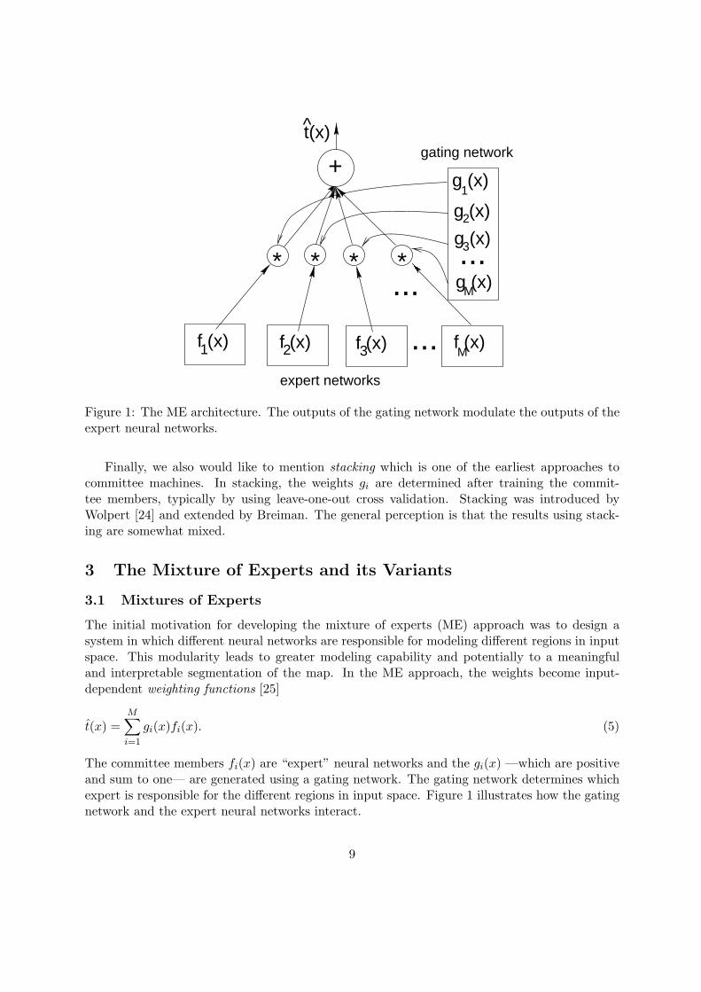
Figure 1: The ME architecture. The outputs of the gating network modulate the outputs of theexpert neural networks.

Finally, we also would like to mention stacking which is one of the earliest approaches tocommittee machines. In stacking, the weights gi are determined after training the commit-tee members, typically by using leave-one-out cross validation. Stacking was introduced byWolpert [24] and extended by Breiman. The general perception is that the results using stack-ing are somewhat mixed.

3 The Mixture of Experts and its Variants

3.1 Mixtures of Experts

The initial motivation for developing the mixture of experts (ME) approach was to design asystem in which different neural networks are responsible for modeling different regions in inputspace. This modularity leads to greater modeling capability and potentially to a meaningfuland interpretable segmentation of the map. In the ME approach, the weights become input-dependent weighting functions [25]

t(x) =M∑i=1

gi(x)fi(x). (5)

The committee members fi(x) are “expert” neural networks and the gi(x) —which are positiveand sum to one— are generated using a gating network. The gating network determines whichexpert is responsible for the different regions in input space. Figure 1 illustrates how the gatingnetwork and the expert neural networks interact.

9

The most important training algorithm for the ME is derived using the following probabilisticassumptions. Given an input x, expert network i is selected with probability gi(x). An outputis generated by adding Gaussian noise with variance σi(x)2 to the output of the expert networkfi(x). Since it is unknown in the data which expert network produced the output, the probabilityof an output given the input is a mixture distribution of the form

P (y|x) =M∑i=1

gi(x) G(y; fi(x), σi(x)2

)which yields E(y|x) =

M∑i=1

gi(x) fi(x),

where G(y; fi(x), σi(x)2

)is the notation for a Gaussian probability density centered at fi(x),

with variance σi(x)2, evaluated at y. By looking at the previous equations, it becomes clear thatthe ME can also be considered to be a flexible model for conditional probability densities [26, 27].Note that in this most general formulation, the outputs of the gating network, the expert neuralnetworks and the noise variance are functions of the input. To ensure that the gi(x) are positiveand sum to one and that the standard deviation is positive one parameterizes

gi(x) =exp hi(x)∑M

j=1 exp hj(x)and σi(x) = exp(si(x))

where the functions hi(x) and si(x) are typically modeled as neural networks. For training theME system, a maximum likelihood error function is used. The contribution of the j-th patternto the log-likelihood function is

lj = logM∑i=1

gi(xj)G(yj ; fi(xj), σi(xj)2

).

Following the derivation in [27], the gradients of lj with respect to the outputs of the variousnetworks become

∂lj∂fi(xj)

= P (i|xj , yj)yj − fi(xj)

σi(xj)2

∂lj∂hi(xj)

= P (i|xj , yj) − gi(xj)

∂lj∂si(xj)

= P (i|xj , yj)

((yj − fi(xj))2

σi(xj)2− 1

)

where the probability that the i-th expert generated data point (xj , yj) is calculated as

P (i|xj , yj) =gi(xj) G

(yj ; fi(xj), σi(xj)2

)∑Mi=1 gi(xj) G (yj ; fi(xj), σi(xj)2)

using the current parameter estimates.The adaptation rules simplify if both hi(x) and fi(x) are linear functions of the inputs [28].

In [29] a variant is described in which both hi(x) and fi(x) are modeled using Gaussian processes.For the fi(x), Gaussian processes with different bandwidths are used such that, input dependent,the expert with the appropriate bandwidth is selected by the gating network.

10

3.2 Extensions to the ME Approach

3.2.1 Hierarchical Mixtures of Experts

The hierarchical mixtures of experts (HMEs) have two (or more) layers of gating networks andtheir output is calculated as

t(x) =M∑i=1

gi(x)N(i)∑j=1

gi,j(x)fi,j(x). (6)

where

gi,j(x) =exp hi,j(x)∑N(i)

j=1 exp hi,j(x).

In the HME, a weighted combination of the outputs of M ME networks is formed. N(i) is thenumber of experts in the i-th ME network. In the HME approach, hi(x), hi,j(x) and fi(x) aretypically linear functions. By using several layers of gating networks in the HME, one obtainslarge modeling flexibility despite the simple linear structure of the expert networks. On theother hand, by using linear models, the HME can be trained using a expectation maximization(EM) algorithm which exhibits fast convergence.

The HME can be seen as a soft decision tree and (hard) decision tree learning algorithms,such as the CART algorithm, can be used to initialize the HME. The HME was developed byJordan and Jacobs [30]. A very extensive discussion of the HME is found in [28].

3.2.2 Alternative Training Procedures

A number of variations of the architecture and the training procedure for the ME have beenreported. The learning procedure of the last section produces competing MEs in the sense thatthe committee members compete for the responsibility for the data. The cooperating MEs areachieved if the squared difference between output data and predictions

∑Kj=1(yj − t(xj))2 is

minimized. Here, the solutions are typically less modular and the model has a larger tendencyto overtraining.

Another variant starts from the joint probability model

P (i)P (x|i)P (y|x, i)

where P (i) is the prior probability of expert i, P (x|i) is the probability density of input x forexpert i and P (y|x, i) is the probability density of y given x and expert i. If we assume that thelatter is modeled as before, we obtain Equation 5 with

gi(x) = P (i|x) =P (i)P (x|i)∑M

j=1 P (j)P (x|j) . (7)

In some applications the experts are trained a priori on different data sets. In this case we canestimate P (i) as the fraction of data used to train expert i, and P (x|i) as the input density ofthe data used to train expert i. In [32] it was suggested to model the latter as a mixture of

11

Gaussians. In [33] and [34], approaches to generating the HME model based on joint probabilitymodels are described.

A very simple ME variant is obtained by modeling the joint input-output probability of(x, y)′ as a mixture of Gaussians. If we calculate the expected value of y given x, we obtainan ME network with linear experts and the gating network of Equation 7 where all conditionalprobability densities are Gaussians. The advantage of this simple variant is that it can bedescribed in terms of simple probabilistic rules which can be formulated by a domain expert.Various combinations of the ME network with domain expert knowledge are described in [31, 33].

3.3 Concluding Remarks

The ME is typically not used if the only goal is prediction accuracy, but is applied in cases whereits unique modeling properties, interpretability and fast learning (in the case of the HME), areof interest. The capability of the ME to model a large class of conditional probability densitiesis useful in the estimation of risk [27], in optimal control and portfolio management [26], andin graphical models [35]. In some applications, the ME has been shown to lead to interestingsegmentations of the map, as in the cognitive modeling of motor control [36].

Of the many generalizations of the ME approach, we want to mention the work of Jacobs andTanner [37] who generalize the ME approach to a wider class of statistical mixture models, i.e.,mixtures of distributions of the exponential family, mixtures of hidden Markov models, mixturesof marginal models, mixtures of Cox models, mixtures of factor models, and mixtures of trees.

4 A Bayesian Committee Machine

Consider the case that a large training data set is available. It is not obvious that a neuralnetwork trained on such a large data set makes efficient use of all the data. It might makemore sense to divide the data set into M data sets, train M neural networks on the data setsand then to combine their predictions using a committee machine (see Figure 2, left). Thisapproach is even more appropriate if the estimators are kernel based systems such as Gaussianprocess regression systems, smoothing splines or support vector machines. Parameter estimationfor those systems requires operation whose computational complexity grows quickly with thesize of the training data set such that those systems are not well suited for large data sets.An obvious solution would be to split the training data set into M data sets, train individualestimators on the partitioned data sets and then combine their predictions. The computationallycomplexity of such an approach grows only linearly with the size of the training data set if Mgrows proportional to the size of the training data set. Important questions are: does oneloose prediction performance by this procedure and what is a good combination scheme. In thissection we analyze this approach from a Bayesian point of view. It turns out that the optimalcombining weights can be calculated based on the covariance structure and that for the optimalprediction of the committee at a given input x, the prediction of the members at inputs otherthan x can be exploited. Note that in previous sections only predictions at x were used in thecommittee machines. A main result of this work is that the quality of the predictions dependscritically on the number of different inputs which contribute to the prediction. If this number is

12

identical to the effective number of parameters then the performance of the committee machineis very close to the performance of one system trained on all data.

This section is different in character than the previous sections. Whereas in previous sections,we provided an overview of the state of the art of the respective topics, this section almostexclusively presents recent results of the author [38, 39].

4.1 Theoretical Foundations

Let x be a vector of input variables and let y be the output variable. We assume that,given a function f(x), the output data are (conditionally) independent with conditional densityP (y|f(x)).

Furthermore, let Xq = xq1, . . . , x

qNQ

denote a set of NQ test points (superscript q for query)and let f q = (f q

1 , . . . , f qNQ

) be the vector of the corresponding unknown response variables. Notethat we query the system at a set of query points (or test points) at the same time which willbe of importance later on.

As indicated in the introduction, we now assume a setting where instead of training oneestimator using all the data, we split up the data into M data sets D = D1, . . . , DM (oftypically approximately same size) and train M estimators on the partitioned training datasets. Let Di = D \ Di denote the data which are not in Di.

Then we have in general2

P (f q|Di, Di) ∝ P (f q)P (Di|f q)P (Di|Di, f q).

Now we would like to approximate

P (Di|Di, f q) ≈ P (Di|f q). (8)

This is not true in general unless f q contains the targets at the input locations of all thetraining data: only then all outputs in the training data are independent. The approximationin Equation 8 becomes more accurate when

• NQ is large — since then f q determines f everywhere

• the correlation between the outputs in Di and Di is small, for example if inputs in thosesets are spatially separated from each other

• when the size of the data set in Di is large since then those data become more independenton average.

Using the approximation and applying Bayes’ formula, we obtain

P (f q|Di−1, Di) ≈ const × P (f q|Di−1)P (f q|Di)P (f q)

(9)

such that we can achieve an approximate predictive density

P (f q|D) = const ×∏M

i=1 P (f q|Di)P (f q)M−1

(10)

2We assume that inputs are given.

13

where const is a normalizing constant. The posterior predictive probability densities are simplymultiplied. Note that since we multiply posterior probability densities, we have to divide bythe priors M − 1 times. This general formula can be applied to the combination of any suitableBayesian estimator.

4.2 The BCM

In the case that the predictive densities P (f q|Di) and the prior densities are Gaussian (or canbe approximated reasonably well by a Gaussian), Equation 9 takes on an especially simple form.Let’s assume that the a priori predictive density at the NQ query points is a Gaussian with zeromean and covariance Σqq and the posterior predictive density for each committee member is aGaussian with mean E(f q|Di) and covariance cov(f q|Di). In this case we achieve [38] (E andcov are calculated with respect to the approximate density P )

E(f q|D) =1C

M∑i=1

cov(f q|Di)−1E(f q|Di) (11)

with

C = cov(f q|D)−1 = −(M − 1)(Σqq)−1 +M∑i=1

cov(f q|Di)−1. (12)

We recognize that the predictions of each committee member i are weighted by the inversecovariance of its prediction. But note that we do not compute the covariance between thecommittee members but the covariance at the NQ query points! This means that predictivedensities at all query points contribute to the prediction of the BCM at a given query point (seeFigure 2, right). This way of combining the predictions of the committee members is namedthe Bayesian committee machine (BCM). An intuitive appealing effect is that by weighting thepredictions of the committee members by the inverse covariance, committee members whichare uncertain about their predictions are automatically weighted less than committee memberswhich are certain about their predictions.

4.3 Experiments

In the experiments, we applied the BCM to Gaussian process regression. Gaussian processregression is particularly suitable since prior and posterior densities are Gaussian distributedand the covariance matrices which are required for the BCM are easily calculated. A shortintroduction into Gaussian process regression can be found in the Appendix.

Figure 3 (right) shows results of applying the BCM to Gaussian process regression for a largeartificial data set [38]. Note that the BCM with K = 60000 training data points achieves resultsunobtainable with simple Gaussian process regression which is limited to a training data set ofapproximately K = 1000.

4.4 Concluding Remarks

The previous discussion on the BCM has focussed on regression. In the form of the generalizedBCM (GBCM), the approach has been extended towards classification, the prediction of counts,

14

DD

E(f |D )

E(f |D )ME(f |D )

MD

^

...3

3E(f |D )2

D2

E(f |D )1

^

1

D

...

weighted combination BCM

q q q q

q

E(f |D )

E(f |D )

E(f |D )M

2

1

E(f |D)q

q

q

q

Figure 2: Left: In the BCM, data sets are partitioned and the committee members estimatethe targets based on the partitioned data sets. The prediction of the committee is formed bya weighted combination of the predictions. Right: In most committee machines, the predictionat a given input is calculated by a combination of the predictions of the committee members atthe same input (vertical continuous line). In the BCM, predictions at other inputs are also used(vertical dashed lines).

15

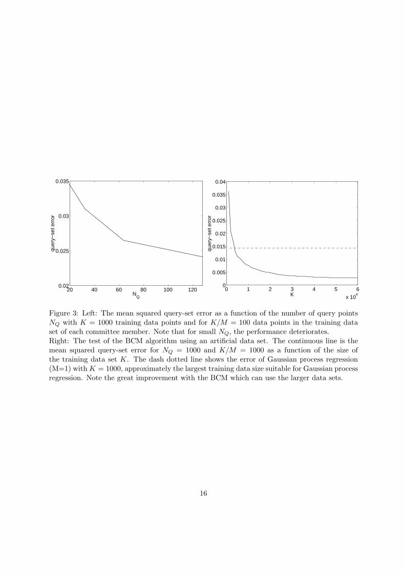
20 40 60 80 100 1200.02

0.025

0.03

0.035

NQ

quer

y−se

t err

or

0 1 2 3 4 5 6

x 104

0

0.005

0.01

0.015

0.02

0.025

0.03

0.035

0.04

K

quer

y−se

t err

or

Figure 3: Left: The mean squared query-set error as a function of the number of query pointsNQ with K = 1000 training data points and for K/M = 100 data points in the training dataset of each committee member. Note that for small NQ, the performance deteriorates.Right: The test of the BCM algorithm using an artificial data set. The continuous line is themean squared query-set error for NQ = 1000 and K/M = 1000 as a function of the size ofthe training data set K. The dash dotted line shows the error of Gaussian process regression(M=1) with K = 1000, approximately the largest training data size suitable for Gaussian processregression. Note the great improvement with the BCM which can use the larger data sets.

16

the prediction of lifetimes, and other applications which can be derived from the exponentialfamily of distributions [39]. The support vector machine is closely related to Gaussian processesand can also be used in the BCM [40]. Furthermore, it is possible to derive online Kalman filterversions of the BCM which only requires one path through the data set and only requires thestorage of a matrix of the dimension of the number of query or test points [38]. After training,the prediction at additional test points only requires resources dependent on the number ofquery points but is independent of the size of the training data set. An interesting questionis how many query points ideally are required. It turns out that the number of query pointsshould be equal to or larger than the effective number of parameters of the map. If this is thecase the query points uniquely define the map (if appropriately chosen) and approximation inEquation 8 becomes an equality [38] (see Figure 3, left).

Since the BCM has the form of a committee machine, it might be possible to further improveperformance by connecting it with ideas from Section 2. The issue of boosting the BCM is afocus of current work.

Finally, it is also possible to derive the BCM solution from a non-Bayesian perspective wherethe covariance matrices are derived from variations over repeated experiments (i.e., variationsover data sets). The goal is to form a linear combination of the predictions at the query points

f qi =

M∑k=1

NQ∑j=1

gi,k(xj)fqk (xj)

such that the expected error is minimum. Here, f qi is the estimate of the committee for input

xi, gi,k(xj) is the weight of query point j of committee member k to predict query point i andf q

k (xj) is the prediction of committee member k for input xj . We use the assumption thatthe individual committee members are unbiased and enforce the constraint that the combinedsystem is unbiased by requiring that

M∑k=1

gi,k(xi) = 1 andM∑

k=1

gi,k(xj) = 0 ∀ j 6= i.

As solution we obtain the BCM with (Σqq)−1 → 0 (negligible prior). Details can be found in [38].

5 Conclusions

The research on committee machines is still very young but has already produced a number of in-teresting architectures and algorithms. Due to the limited space, we naturally could not providea comprehensive overview covering all aspects of committee machines. As examples, boost-ing has been analyzed from the perspectives of PAC-learning, game theory and “conventional”statistics. Furthermore, committee machines have been applied to density estimation [41, 42],hidden Markov models and a variety of statistical mixture models. Also, we completely left outapproaches to committee machines originating from statistical physics and modular approachesfor sensory fusion and control. Finally, there are interesting common aspects between committeemachines and biological systems: Committee machines, in general, are very tolerant versus thebreakdown of any of its components and, similarly to biological systems, system performance

17

only deteriorates dramatically if a large number of committee members (as neural modules) aremalfunctioning.

In their many facets, committee machines have made important contributions to variousbranches of neural computation, machine learning, and statistics and are becoming increasinglypopular in the KDD-community. They have opened up a new dimension in machine learningsince committees can be formed using virtually any prediction system. As demonstrated by thenumerous contributions from various communities, committee machines can be understood andanalyzed from a large number of different view points, often revealing new interesting insights.We can expect numerous novel architectures, algorithms, applications and theoretical insightsfor the future.

Acknowledgements

Valuable comments by Salvatore Ingrassia and Michal Skubacz are greatfully acknowledged.

6 Appendix: Gaussian Process Regression

In contrast to the usual parameterized approach to regression, in Gaussian process regressionwe specify the prior model directly in function space. In particular, we assume that a priori f isGaussian distributed (in fact it would be an infinite-dimensional Gaussian) with zero mean anda covariance cov(f(x1), f(x2)) = σx1,x2 . We assume that we can only measure a noisy versionof f

y(x) = f(x) + ε(x)

where ε(x) is independent Gaussian distributed noise with zero mean and variance σ2ψ(x).

Let (Σmm)ij = σxmi ,xm

jbe the covariance matrix of the measurements, Ψmm = σ2

ψ(x)I bethe noise variance between the outputs, (Σqq)ij = σxq

i ,xqj

be the covariance matrix of the querypoints and (Σqm)ij = σxq

i ,xmj

be the covariance matrix between training data and query data. I

is the K-dimensional unit matrix.Under these assumptions, the conditional density of the response variables at the query

points is Gaussian distributed with mean

E(f q|D) = Σqm(Ψmm + Σmm)−1ym, (13)

and covariance

cov(f q|D) = Σqq − Σqm (Ψmm + Σmm)−1 (Σqm)′. (14)

Note that for the i−th query point we obtain

E(f qi |D) =

K∑j=1

σxqi ,xm

jvj (15)

where vj is the j−th component of the vector (Ψmm + Σmm)−1ym. The last equation describesthe weighted superposition of kernel functions bj(x

qi ) = σxq

i ,xmj

which are defined for each train-ing data point and is equivalent to some solutions obtained for kriging, regularization neural

18

networks and smoothing splines. The experimenter has to specify the positive definite covariancematrix. A common choice is that σxi,xj = exp(−1/(2γ2)||xi − xj ||2) with γ > 0 such that weobtain Gaussian basis functions, although other positive definite covariance functions are alsoused.

References

[1] Sharkey, A. J. C., Combining artificial neural nets, Springer, 1999.

[2] Granger C. W. J., Combining forecasts-twenty years later, Journal of forecasting, 8, 167,1989.

[3] Bernardo, J. M., and Smith, A. F. M., Bayesian theory, New York: J. Wiley & Sons, 1993.

[4] Quinlan, J. R., Thirteenth National Conference on Artificial Intelligence (AAAI-96) AAAIpress, 1996.

[5] Meir, R., Bias, Variance and the Combination of Least Squares Estimators. in Advances inNeural Information Processing Systems 7, Tesauro, G., Touretzky, D. S., and Leen T. K.,Eds., MIT Press, 295, 1995.

[6] Taniguchi, M. and Tresp, V., Averaging regularized estimators, Neural Computation, 9,1163, 1997.

[7] Breiman, L., Combining predictors, in Combining artificial neural nets, Sharkey, A. J. C.,Ed., Springer, 31, 1999.

[8] Perrone, M. P., Improving regression estimates: averaging methods for variance reductionwith extensions to general convex measure optimization, PhD thesis, Brown University,1993.

[9] Krogh, A. and Vedelsby, J., Neural network ensembles, cross validation, and active learning,in Advances in Neural Information Processing Systems 7, Tesauro, G., Touretzky, D. S.,and Leen T. K., Eds., MIT Press, 231, 1995.

[10] Dietterich, T. G., An experimental comparison of three methods for constructing ensemblesof decision trees: bagging, boosting and randomization, Machine Learning, 40, 130, 2000.

[11] Breiman, L., Randomizing outputs to increase prediction accuracy, Machine Learning, 40,229, 2000.

[12] Raviv, Y., and Intrator, N., Variance reduction via noise and bias constraints, in Combiningartificial neural nets, Sharkey, A. J. C., Ed., Springer, 31, 1999.

[13] Friedman J., Hastie T., and Tibshirani, R., Additive logistic regression: a statistical viewof boosting, Annals of Statistics, to appear.

[14] Schapire R. E., The strength of weak learnability, Machine Learning, 5, 197, 1990.

19

[15] Freund Y. and Schapire R. E., Experiments with a new boosting algorithm, in MachineLearning: Proceedings of the Thirteenth International Conference, 148, 1996.

[16] Zemel, R. S. and Pitassi, T., A gradient-based boosting algorithm for regression problems,in Advances in Neural Information Processing Systems 13, Leen, T. K., Dietterich, T. G.,and Tresp V., Eds., MIT press, 2001.

[17] Schapire R. E., Freund Y., Bartlett P., and Lee, W. S. Boosting the margin: A new expla-nation for the effectiveness of voting methods, The Annals of Statistics, 1651, 1998.

[18] Drucker, H., Boosting neural networks, in Combining artificial neural nets, Sharkey, A. J.C., Ed., Springer, 31, 1999.

[19] Ratsch, G., Onoda, T., and Muller, K.-R., Regularizing AdaBoost, in Advances in NeuralInformation Processing Systems 11, Kearns, M. S., Solla, S. A., and Cohn, D. A. Eds., MITPress, 564, 1999.

[20] Ratsch, G., Scholkopf, B., Smola, A., Muller, K.-R., Onoda, T., and Mika, A., ν-Arc:ensemble learning in the presence of noise, in Advances in Neural Information ProcessingSystems 12, Solla, S. A., Leen T. K., and M ”uller, K. R. Eds., MIT Press, 561, 2000.

[21] Schapire, R. E. and Singer, Y., Improved boosting algorithms using confidence-rated pre-dictions, in Proceedings of the eleventh annual conference on computational learning theory,1998.

[22] Breiman, L., Predicting games and arcing algorithms, TR. 504, Statistics Department,University of California, December, 1997.

[23] Mason, L., Baxter, J., Bartlett, P., and Frean, M., Boosting algorithms as gradient descent,in Advances in Neural Information Processing Systems 12, Solla, S. A., Leen T. K., andMuller, K. R. Eds., MIT Press, 512, 2000.

[24] Wolpert, D. H., Stacked generalization, Neural Networks, 5, 241, 1992.

[25] Jacobs, R. A., Jordan, M. I., Nowlan, S. J., and Hinton, J. E., Adaptive mixtures of localexperts, Neural Computation, 3, 79, 1991

[26] Neuneier, R. F., Hergert, W., Finnof, W., and Ormoneit, D., Estimation of conditionaldensities: a comparison of approaches, Proceedings of ICANN*94, Springer, 1, 689, 1994.

[27] Bishop, C. M., Neural neural networks for pattern recognition, Oxford: Clarendon Press,1995.

[28] Haykin, S., Neural Networks, a comprehensive foundation, 2nd edition, Prentice Hall, 1999.

[29] Tresp, V., Mixtures of Gaussian processes, in Advances in Neural Information ProcessingSystems 13, Leen, T. K., Dietterich, T. G., and Tresp V., Eds., MIT press, 2001.

[30] Jordan, M. I., and Jacobs, R. A., Hierarchical mixtures of experts and the EM algorithm,Neural Computation, 6, 181, 1994.

20

[31] Tresp, V., Hollatz, J., and Ahmad, S., Network structuring and training using rule-basedknowledge, in Advances in Neural Information Processing Systems 5, Giles, C. L., HansonS. J., and Cowan J. D., Eds., Morgan Kaufman, 871, 1993.

[32] Tresp, V., and Taniguchi, M., Combining estimators using non-constant weighting func-tions, in Advances in Neural Information Processing Systems 7, Tesauro, G., Touretzky, D.S., and Leen T. K., Eds., MIT Press, 419, 1995.

[33] Tresp, V., Hollatz, J., and Ahmad, S., Representing Probabilistic Rules with Networks ofGaussian Basis Functions, Machine Learning, 27, 173, 1997.

[34] Xu, L., Jordan, M. I., and Hinton, G. E., An alternative model for mixtures of experts, inAdvances in Neural Information Processing Systems 7, Tesauro, G., Touretzky, D. S., andLeen T. K., Eds., MIT Press, 633, 1995.

[35] Hofmann, R. and Tresp, V., Discovering structure in continuous variables using Bayesiannetworks, in Advances in Neural Information Processing Systems 8, Touretzky, D. S., Mozer,M. C., and Hasselmo, M. E., Eds., MIT Press, 500, 1996.

[36] Brashers-Krug, T., Shadmehr, R., and Todorov, E., M., and Jacobs, R., Catastrophicinference in human motor learning, in Advances in Neural Information Processing Systems7, Tesauro, G., Touretzky, D. S., and Leen T. K., Eds., MIT Press, 19, 1995.

[37] Jacobs, R. and Tanner, M., Mixtures of X, in Combining artificial neural nets, Sharkey, A.J. C., Ed., Springer, 31, 1999.

[38] Tresp, V., The Bayesian committee machine, Neural Computation, 12, 2000.

[39] Tresp, V., The generalized Bayesian committee machine, Proceedings of the Sixth ACMSIGKDD International Conference on Knowledge Discovery and Data Mining, KDD-2000,130, 2000.

[40] Schwaighofer, A., and Tresp, V., The Bayesian committee support vector machine,manuscript, submitted for publication, 2001.

[41] Ormoneit, D. and Tresp, V., Averaging, maximum penalized likelihood and Bayesian esti-mation for improving Gaussian mixture probability density estimates, IEEE Transactionson Neural Networks, 9, 639, 1998.

[42] Smyth, P., and Wolpert, D., Stacked density estimation, in Advances in Neural InformationProcessing Systems 10, Jordan, M. I., Kearns, M. J., and Solla A. S., Eds., MIT Press, 668,1998.

21