combined lidar and radar observations of vertical motions ... · penetrated completely by both...
TRANSCRIPT

Combined lidar and radar observations ofvertical motions and heterogeneous iceformation in mixed-phase layered clouds
Field studies and long-term monitoring
Der Fakultat fur Physik und Geowissenschaftender Universitat Leipzig
eingereichte
Dissertation
zur Erlangung des akademischen Grades
Doctor rerum naturalium(Dr. rer. nat.)
vorgelegt
von Diplom-Physiker Johannes Buhlgeboren am 21. September 1983 in Reutlingen
Leipzig, den 25. September 2014

Contents
Contents 3
1 Introduction 5
2 Heterogeneous ice formation: The role of vertical air motions 92.1 Interactions between aerosols, atmospheric dynamics and clouds . . . . . 92.2 Active versus passive remote sensing of clouds . . . . . . . . . . . . . . . 102.3 Review of recent literature on the theory of mixed-phase cloud parcels . . 112.4 Connecting observations with simulations . . . . . . . . . . . . . . . . . . 162.5 Arising questions . . . . . . . . . . . . . . . . . . . . . . . . . . . . . . . 18
3 Lidar and radar synergy. Part I: Signal strength 193.1 Description of lidar and radar backscattering . . . . . . . . . . . . . . . . 193.2 Detection of spherical and non-spherical particles with lidar and radar . . 25
4 TROPOS remote-sensing facility for simultaneous profiling of aerosols,clouds and meteorological parameters 314.1 Instrument overview . . . . . . . . . . . . . . . . . . . . . . . . . . . . . 314.2 Measurement example . . . . . . . . . . . . . . . . . . . . . . . . . . . . 334.3 Measurement strategy for the UDINE campaign at Leipzig (2010–2013) . 354.4 LACROS data storage and processing . . . . . . . . . . . . . . . . . . . . 364.5 Mixed-phase cloud classification scheme . . . . . . . . . . . . . . . . . . . 38
5 Lidar and radar synergy. Part II: Vertical-velocity measurement with Dopplerlidar, cloud radar and wind profiler 415.1 Doppler wind lidar . . . . . . . . . . . . . . . . . . . . . . . . . . . . . . 415.2 Cloud-radar data processing . . . . . . . . . . . . . . . . . . . . . . . . . 565.3 Linking Doppler lidar and cloud radar . . . . . . . . . . . . . . . . . . . 575.4 Capabilities of lidar and radar to probe turbulence . . . . . . . . . . . . 605.5 Combined observations with Doppler lidar, cloud radar and wind profiler 62
6 Vertical-velocity and glaciation statistics of mid-latitude and sub-tropicallayered clouds 716.1 Overview about UDINE and SAMUM campaigns . . . . . . . . . . . . . 716.2 Case studies from UDINE . . . . . . . . . . . . . . . . . . . . . . . . . . 756.3 Observation of cloud freezing with LACROS . . . . . . . . . . . . . . . . 806.4 Quantification of heterogeneous ice formation in mixed-phase layered clouds 84
3

6.5 Combined lidar/radar vertical-wind statistics in layered clouds . . . . . . 88
7 Towards the measurement of ice-particle flux from cloud-radar spectra 1017.1 A measure for the particle nucleation rate accessible by remote sensing . 1027.2 Deriving ice-particle flux from cloud-radar spectra . . . . . . . . . . . . . 1047.3 Preparation of cloud-radar spectra . . . . . . . . . . . . . . . . . . . . . 1057.4 Case studies . . . . . . . . . . . . . . . . . . . . . . . . . . . . . . . . . . 1077.5 Size separation of particles . . . . . . . . . . . . . . . . . . . . . . . . . . 1157.6 Discussion of errors and scope of the method . . . . . . . . . . . . . . . . 115
8 Summary, conclusions and outlook 1198.1 Summary and conclusions . . . . . . . . . . . . . . . . . . . . . . . . . . 1198.2 Outlook . . . . . . . . . . . . . . . . . . . . . . . . . . . . . . . . . . . . 121
Bibliography 125
List of symbols 137
List of abbreviations 141
4
1 IntroductionClouds always cover about two thirds of the Earth’s surface. They thus determine theEarth’s albedo to a high degree and are an important regulator of the global radiationbalance. Therefore, they pose a crucial component in numeric climate projections. Evensmall errors in the knowledge about physical composition and global distribution ofclouds can lead to high uncertainties in the estimation of the human impact on thepresently observed change in global climate.
In the last report of the Intergovernmental Panel on Climate Change (IPCC) aerosol-cloud interactions (ACI) were identified as one of the most uncertain components ofhuman climate impact [Boucher et al., 2014]. The direct influence of aerosol propertieson clouds [Twomey, 1977] and the numerous fast adjustments [Albrecht, 1989] of thecloud systems are estimated to create an effective radiative forcing of −0.45 W m−2,but with an uncertainty of around 100%. At present state of knowledge, changes incloud properties seem to be one of the strongest components counteracting the radiativeforcing of +1.68 W m−2 introduced by human CO2 emissions.
Comparisons between model outputs and satellite observations showed that the predic-tion of clouds is still fairly inaccurate [Zhang et al., 2010b]. There is a considerable lackof process-level understanding, especially for mixed-phase clouds which contain liquidwater and ice particles at the same time. Within and around such mixed-phase clouds acomplex interplay between aerosols, water and air motions takes place. The Leibniz In-stitute for Tropospheric Research at Leipzig (TROPOS) has been active in investigatingaerosols and clouds since the foundation of the institute in the year 1992. Aerosol fluxesinto clouds [Engelmann et al., 2008; Schmidt et al., 2013] and long-range aerosol trans-port [Baars et al., 2011; Groß et al., 2011; Muller et al., 2005] have been explored alongwith mixed-phase cloud freezing processes [Ansmann et al., 2005, 2009; Seifert et al.,2010; Kanitz et al., 2011] by means of lidar remote sensing. Activities of other groupson this topic include lidar measurements in arctic mixed-phase clouds [de Boer et al.,2009] and aircraft measurements in mixed-phase mid-level clouds [Fleishauer et al., 2002;Noh et al., 2012; Korolev and Isaac, 2006; McFarquhar et al., 2013]. The CloudSat andCALIPSO (Cloud-Aerosol Lidar and Infrared Pathfinder Satellite Observations) satel-lites are used for combined lidar/radar measurements from space to probe the cloud topheight and the properties of falling ice particles below the cloud at the same time [Zhanget al., 2010a,b]. In the context of this work, “cloud top” and “cloud base” refer to thevertical extent of the predominantly liquid top of a cloud layer. The height range belowthis top layer, where particles may deposit, is called “virga”.
Air- and spaceborne measurement techniques at the same time have their limitations.Aircraft can deliver unique measurements of liquid water and ice crystals, but they canonly measure at one height at the same time. They can either observe ice formation at
5

cloud top or the resulting ice crystals at cloud base. Also flying through supercooledliquid- or mixed-phase layers is difficult because of aircraft and instrument icing. Fromspace, a detailed look into the processes and the determination of specific particle prop-erties is not possible.
The recent efforts brought insight into the effects that aerosol particles have on clouds.But the dynamics of the aerosol-cloud interaction is still poorly understood [Morrisonet al., 2012]. Information about air movement in and around the clouds are largely ab-sent, although air motions mediate the interaction between aerosols and cloud droplets.Gravity waves can create a cloud, turbulence can entrain aerosol particles in and out ofa cloud. Small-scale vertical movements lead to regular changes in water-vapor super-saturation controlling the evaporation and growth of cloud droplets. The role of verticalair motions and turbulence in the formation of ice particles and in the regulation of theWegener–Bergeron–Findeisen (WBF) process has been found to be unclear by Korolev[2007]. However, any approach to this problem is hampered by the absence of measure-ments giving direct and quantitative information about vertical motions in the vicinityof clouds. The following chapter gives an overview about this problem.
For the continuous observation of aerosols, clouds and their interactions TROPOSbuilt the multi-instrument measurement platform LACROS (Leipzig Aerosol and CloudRemote Observations System). LACROS combines the abilities of advanced Raman/pol-arization lidars [Althausen et al., 2000, 2009; Mattis et al., 2004], a cloud radar, a Dopplerlidar [Engelmann et al., 2008; Buhl et al., 2012], a microwave radiometer [Rose et al.,2005] and several auxiliary measurement systems to provide important parameters ofaerosol and cloud layers simultaneously. Its lidars mainly sense aerosol particles andsmall droplets at predominantly liquid cloud bases. The cloud radar delivers informa-tion about the presence and the properties of large ice particles falling in the virgae.The difference between the lidar and radar systems is analyzed in detail in Chapter 3.LACROS as a whole is described in Chapter 4.
The combination of lidars and radars is used here for the first time to draw a coherentpicture of the processes within turbulent cloud layers in the middle troposphere. Inthis way, height, phase (liquid, mixed-phase or ice) and vertical velocity at cloud basesof mid-level layered clouds are probed simultaneously. Layered clouds are ideal targetsfor the observation and investigation of cloud-droplet freezing processes. They can bepenetrated completely by both lidar and radar and show narrow constraints on environ-mental variables like pressure and temperature. Knowledge about the complete verticalwind field around such a cloud system and inside its turbulent layers is needed for thequantification and understanding of the physical processes. Large-scale vertical motionsare important for the generation of clouds (e.g., gravity waves). Small-scale turbulence isthe dominant driver for the microphysics within a cloud layer. Formation of ice crystalsvia contact or immersion freezing, the generation of large droplets, support or inhibitionof the WBF process and the recreation of liquid drops in the presence of ice crystalscritically depend on vertical air motion [Korolev and Isaac, 2003].
This work aims in particular at the integration of Doppler lidar data into continuousmeasurements and field campaigns of TROPOS with LACROS. Despite the need forthose measurements, there is currently no measurement instrument that is specifically
6
1. Introduction
designed to measure vertical wind fields at cloud base. Cloud radars simply do not sensethe small droplets, and the signal from Doppler lidars is contaminated by artifacts causedby the large signal gradient at cloud base and the laser pulse chirp. In Chapter 5, meth-ods are introduced to reduce these artifacts and accurately derive vertical air velocityin the vicinity of clouds, especially at cloud bases. These methods have been developedin the framework of this thesis. In Chapter 5, also the results of a small measurementcampaign conducted at the Meteorological Observatory Lindenberg (MOL, Germany)are shown. Lidars and cloud radars can measure the vertical wind field inside, but usu-ally not around cloud layers due to the absence of tracer targets. The air motion itself,however, can be sensed by wind profilers exploiting Bragg scattering in clear air [Strauchet al., 1984]. In a cooperative effort between TROPOS and the German MeteorologicalService (DWD, Deutscher Wetterdienst), simultaneous operation of a wind profiler, aDoppler lidar and a cloud radar was tested at MOL for the first time. This uniquecombination of instruments allows the independent observation of large-scale air mo-tion, small-scale turbulence and particle fall velocities inside complex cloud scenes. Theeffort was motivated by experience from measurements with LACROS and is intendedto show a way towards obtaining the complete picture of vertical motions in the vicinityof clouds.
A comprehensive statistics of vertical motion patterns at cloud base was collectedwith Doppler lidar during the UDINE (Up- and Downdrafts in Drop and Ice NucleationExperiment, Leipzig, 2010–2013) and SAMUM-2 (Saharan Mineral Dust Experiment,Cape Verde, 2008) projects, offering the unique opportunity to compare mid-latitudinaland sub-tropical layered clouds. Combined with the simultaneous measurements ofpowerful polarization lidars (UDINE and SAMUM-2) and a cloud radar (UDINE), acomprehensive look into the processes of ice formation and vertical motion is possiblefor the first time. In Chapter 6, the statistics of vertical velocity at cloud bases ispresented together with the simultaneously measured properties of ice crystals fallingfrom the cloud base. Basic ice cloud properties (e.g., ice-water content) are evaluatedwith classic and proven methods [e.g., Hogan et al., 2006]. In Chapter 7, a new methodis proposed to measure the flux of ice crystals through cloud base to get an idea of thenucleation efficiency in cloud layers. The particle size spectra necessary for this approachare derived from radar spectra based on the terminal fall velocities of ice crystals. Theproposed method relies on a combination of Doppler lidar, cloud radar and wind profilerto retrieve the true terminal fall velocity of the particles relative to the surrounding air.Chapter 8 summarizes the work and gives an outlook on further steps to be taken.
7


2 Heterogeneous ice formation: Therole of vertical air motions
2.1 Interactions between aerosols, atmosphericdynamics and clouds
The IPCC report 2013 states that “clouds and aerosols continue to contribute the largestuncertainty to estimates and interpretations of the Earth’s changing energy budget”.Clouds and aerosols cannot be treated independently, because aerosols acting as cloudcondensation nuclei (CCN) are an abundant resource present in any place where a watercloud may form. Once activated, the cloud droplet in turn changes the chemical andphysical properties of the CCN and influences its ability to form again a new dropletafter evaporation. Activation and a possible subsequent freezing of water droplets canonly occur, if supersaturation over liquid water is reached. Two possible ways towardssupersaturation are radiative cooling of moist air or vertical movement leading to atemperature drop and hence a rise in relative humidity above the water-vapor super-saturation level. The actual freezing behavior of liquid droplets is then governed by aneven more mysterious form of aerosols – the ice nuclei (IN). They only make up a verytiny fraction of all particles in the air, but at temperatures above −38 C the presenceof IN is required for droplet freezing and cloud glaciation. DeMott et al. [2010] showedthat at −20 C the fraction of IN in all aerosol particles larger than 0.5 µm in diameteris on average 10−3. The temperature at which glaciation occurs is strongly connectedwith the IN composition [Stratmann et al., 2004; Hartmann et al., 2013; Phillips et al.,2013] and hence with their geographic origin [Seifert et al., 2010].
Both transport of aerosols and the formation of clouds can be observed in the at-mosphere by means of remote sensing [Seifert et al., 2010; Kanitz et al., 2011]. Butonce a cloud has formed, the physical processes are usually hidden inside of the cloudlayer in a mostly turbulent environment. The partitioning of liquid droplets and iceparticles is thus difficult and one of the main reasons why the process-level understand-ing of mixed-phase clouds is low. However, for precise climate projections process-levelunderstanding is critical, because phenomenological parameterizations solely based onpresent-day observations may loose their validity in future due to changes in the envi-ronmental conditions.
The complexity of mixed-phase clouds cannot be resolved by a single measurementsystem alone but needs combined measurements that probe different parameters at once.Already now it is clear that it will take years of continuous measurements all overthe world to unravel the in-cloud processes in sufficient detail to make accurate cloud
9

predictions. Mixed-phase cloud processes play a role in different kind of clouds butaccurate measurements are difficult. Lidars, e.g., cannot penetrate to the center of aconvective thunderstorm cloud where even for radars signal attenuation is so strong thatquantitative use of the signal is very limited. As measurement values from thin layeredclouds are most easy to obtain and to evaluate, they are a good starting point for thekind of study carried out in this work.
While the challenging interaction between aerosol particles and cloud droplets posesa lot of unknowns, abundant and promising research is going on in this field [Hartmannet al., 2011; Chernoff and Bertram, 2010]. First-hand information about in-cloud tur-bulence however is virtually absent. Some aircraft studies [Fleishauer et al., 2002; Fieldet al., 2004] are present, but the observation is usually restricted to a few cases. Thiswork aims at filling this gap for tropospheric mid-level layered clouds in the mid-latitudesand the sub-tropics. For that purpose, the first three years of LACROS observations atLeipzig are evaluated together with measurements from the SAMUM-2 campaign thattook place at Praia, Cape Verde.
2.2 Active versus passive remote sensing of cloudsActive remote sensing with lidar and radar can yield precise information about the stateof the atmosphere in general and about the properties of clouds in particular. The timeand height resolution is usually on the order of seconds and tens of meter, respectively.For this work, the height, temperature, liquid/ice mixing state and vertical velocity atcloud base have to be collected simultaneously for each layered cloud under study. Pas-sive remote-observation instruments like hyperspectral instruments on satellites provideinformation from a much wider field of view, deliver basic microphysical properties ofclouds and allow some estimations of cloud top height. For the determination of thephysical state of a layered cloud, active remote sensing allows for much more reliableand direct information. Ambiguities in the determination of height are smaller and icecrystals falling through the cloud base can be detected and classified unambiguously.Moreover, Doppler lidars or cloud radars even provide the only known methods to po-tentially determine vertical velocity at cloud base.
Figure 2.1a shows the satellite image of a cloud scene over Leipzig and the correspond-ing Doppler lidar and cloud radar measurements made at TROPOS around the sametime. While the passive satellite cameras can only detect the mere presence of a cloud,the Doppler lidar and cloud radar at TROPOS detect strong vertical movements of upto ±0.5 m s−1 at the top of the cirrus layer. Below the high cirrus clouds, smaller lay-ers of mid-level clouds become visible around 6:00 UTC (Coordinated Universal Time)showing up- and downdrafts alternating in the range of ±1.0 m s−1 on a much smallertime scale. By the time the cloud has moved over TROPOS, it may have changed, butthe statistical behavior of the vertical motions may be representative for the cloud scenecaptured by the satellite. The example from Fig. 2.1 shows, how the combination ofdifferent remote-sensing instruments can upvalue the single systems.
Already in Fig. 2.1 the different sensitivities of Doppler lidar and cloud radar are
10

2. The role of vertical air motions
Ver
tical
Vel
ocity
[m s⁻¹
]
Hei
ght [
m]
Ver
tical
Vel
ocity
[m s⁻¹
]
Hei
ght [
m]
-40
20
0
-20
Visible Light RGB Composit Infrared Channel
LeipzigLeipzig
Visible Light RGB Composit Infrared Channelb)
HalleHalleLeipzigLeipzig
HalleHalle
a)
c)
altocumulus clouds
cirrus clouds
altocumulus clouds
cirrus clouds
Doppler Lidar
Cloud Radard)
Tem
pera
ture
[°C
]
Figure 2.1: Visible-light (a) and infrared-light (b) satellite measurements taken at 9:21 UTCon 22 May 2013 are shown together with the corresponding Doppler lidar (c) and cloud radar(d) measurements between 6:00 and 8:38 UTC (Image Credit: United States Geological Survey).Positions of cloud layers are marked by the blue (high-level clouds) and red boxes (mid-levelclouds). The measurement quantities of the single systems are discussed in Chapter 3.
visible. The high-level cirrus clouds (blue boxes) detected by the cloud radar are onlypartly visible in the Doppler lidar plots. On the other hand, the Doppler lidar detectsthe altocumulus (AC) cloud (red box) some minutes earlier.
2.3 Review of recent literature on the theory ofmixed-phase cloud parcels
The microphysics of a mixed-phase cloud is dominated by the interplay between aerosols,water droplets, ice crystals and water vapor. At temperatures below 0 C humid air hasa slightly lower saturation vapor pressure over ice than over liquid water. If both liquidwater and ice are present in a stationary air parcel, this leads to an evaporation of theliquid droplets and to a simultaneous growth of the ice crystals. This basic microphysicalbehavior of such a mixed-phase air parcel was first described a century ago by Wegener
11

[1911], Bergeron [1935] and Findeisen [1938] and is consequently called the Wegener–Bergeron–Findeisen (WBF) process.
2.3.1 Glaciating time of a mixed-phase cloudA mixed-phase air parcel which does not move vertically and does not lose ice viadeposition will eventually reach an equilibrium state with only ice crystals present. Thisbasic consequence of the WBF theory contradicts observations in nature where mixed-phase cloud layers are observed to maintain their mixed-phase state over hours [Ansmannet al., 2009]. Korolev and Mazin [2003] showed that even small vertical velocities cansignificantly increase the glaciating time. In Fig. 2.2 the time until complete glaciationfor a cloud parcel with a constant liquid water content (LWC), but different water-dropletnumber concentrations and mean droplet sizes is shown in dependence of vertical velocity.For an air parcel in rest the glaciating time is about 200 s, an updraft of 0.5 m s−1
already leads to a doubling of this value. However, after a certain time equilibrium willbe reached and the formerly mixed-phase cloud will have glaciated completely.
Gla
ciat
ing
Tim
e [s
]
0
200
400
600
800
1000
1200
1400
Vertical Velocity uz [m s⁻¹]−4 −2 0 2 4
N = 1 cm⁻³, r0 = 30 µmN = 10 cm⁻³, r0 = 13 µmN = 100 cm⁻³, r0 = 6.5 µm
Figure 2.2: Glaciating time of a cloud parcel for different realistic cloud droplet and ice crystalconfigurations. The LWC is constant at 0.1 g kg−1. N is the number concentration and r0 theinitial size of the water droplets at the begin of the simulation. The number of ice crystals isNi = 1 cm−3, IWC is zero at the beginning, temperature is T = −10 C. (Figure reproduced fromKorolev and Mazin [2003].)
2.3.2 Supersaturation in a vertically moving mixed-phase cloudparcel
The analytical treatment of the supersaturation in cloud parcels goes back to Squires[1952]. In Korolev and Field [2008] the “effect of dynamics on mixed-phase clouds” isanalyzed and it is shown that a turbulent layered cloud can maintain its mixed-phase
12

2. The role of vertical air motions
composition by constantly recreating liquid water from the vapor phase via upward mo-tion. If an air parcel is ascending fast enough, the vapor pressure can surpass saturationover liquid water. CCN will then instantly activate liquid droplets which will eventuallyevaporate again when the parcel is no longer ascending fast enough. If the air parcel isin harmonic oscillatory motion, the ice crystals will grow during ascent and — if liquiddroplets are present — even a short period during descent. During descent, the icecrystals will evaporate and release water vapor, which will facilitate the re-activation ofliquid droplets during the next ascent. The supersaturation over liquid water Sw in amixed-phase cloud parcel displaced vertically with constant velocity uz can be describedby the differential equation [Korolev and Mazin, 2003]
1
Sw + 1
dSwdt
= a0uz − a2B∗iNiri − (a1BwNwrw + a2BiNiri)Sw. (2.1)
The particle size distribution is assumed to be monodisperse. Ni, Nw, ri and rw arethe corresponding number concentrations and particle radii for ice and water, respec-tively. a0, a1, a2, Bi, B
∗i and Bw are constants holding thermodynamic parameters like
temperature and latent heat of fusion. For a detailed description please refer to Korolevand Mazin [2003]. Eq. (2.1) is the mathematical representation of the WBF process. a0
is a positive constant, so a source of water vapor is created on the right-hand side of theequation, if an air parcel is moving upwards (uz > 0). The other terms represent thepresence of ice crystals and liquid droplets and act as sinks of water vapor. Korolev andMazin [2003] also show that Eq. (2.1) has the solution
Sw =Sqsw − C0 exp(−t/τp)
1 + C0 exp(−t/τp), (2.2)
with
Sqsw =a0uz + b∗iNiri
bwNwrw + biNiri(2.3)
and
τp =1
a0uz + bwNwrw + (bi + b∗i )Niri. (2.4)
τ is the time of phase relaxation, describing the time until the air parcel has reachedagain its original phase state. C0 holds the start parameters and bw, bi and b∗i holdthermodynamic constants. Values of the constants are given in Korolev and Mazin[2003]. Equation (2.2) is called the “quasi-steady solution”, valid only if assumed thatneither liquid nor ice particles change in size and environmental conditions are constant– in general a somewhat unrealistic assumption. However, as layered clouds have a smallvertical extent and consequently do not involve deep convection, Eq. (2.2) can be usefulto depict basic processes within the cloud layer. For t→∞, Sqsw will be the equilibriumsupersaturation of the air parcel. To maintain a liquid phase, Sqsw must be ≥ 0. From
13
Swater saturation
ice saturation
h(z)
uz>u
z*
uz=u
z*
uz → 0
ΔZ*
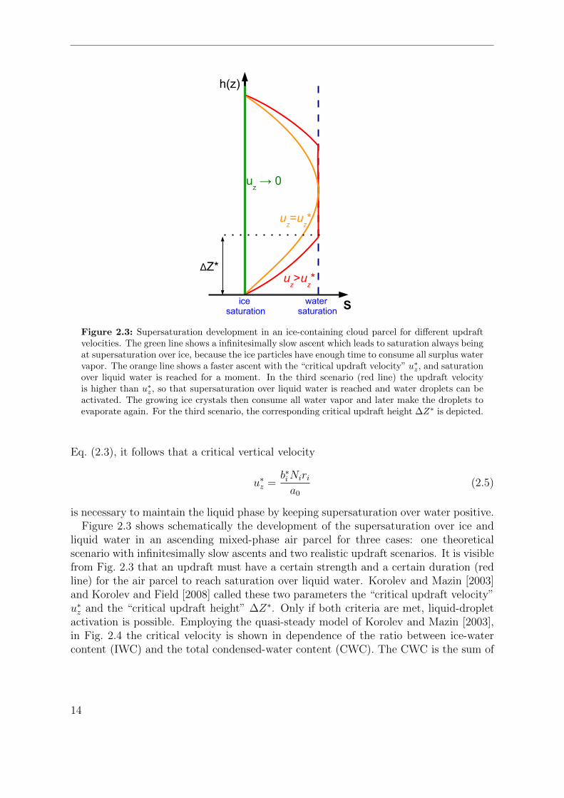
Figure 2.3: Supersaturation development in an ice-containing cloud parcel for different updraftvelocities. The green line shows a infinitesimally slow ascent which leads to saturation always beingat supersaturation over ice, because the ice particles have enough time to consume all surplus watervapor. The orange line shows a faster ascent with the “critical updraft velocity” u∗z, and saturationover liquid water is reached for a moment. In the third scenario (red line) the updraft velocityis higher than u∗z, so that supersaturation over liquid water is reached and water droplets can beactivated. The growing ice crystals then consume all water vapor and later make the droplets toevaporate again. For the third scenario, the corresponding critical updraft height ∆Z∗ is depicted.
Eq. (2.3), it follows that a critical vertical velocity
u∗z =b∗iNiria0
(2.5)
is necessary to maintain the liquid phase by keeping supersaturation over water positive.Figure 2.3 shows schematically the development of the supersaturation over ice and
liquid water in an ascending mixed-phase air parcel for three cases: one theoreticalscenario with infinitesimally slow ascents and two realistic updraft scenarios. It is visiblefrom Fig. 2.3 that an updraft must have a certain strength and a certain duration (redline) for the air parcel to reach saturation over liquid water. Korolev and Mazin [2003]and Korolev and Field [2008] called these two parameters the “critical updraft velocity”u∗z and the “critical updraft height” ∆Z∗. Only if both criteria are met, liquid-dropletactivation is possible. Employing the quasi-steady model of Korolev and Mazin [2003],in Fig. 2.4 the critical velocity is shown in dependence of the ratio between ice-watercontent (IWC) and the total condensed-water content (CWC). The CWC is the sum of
14
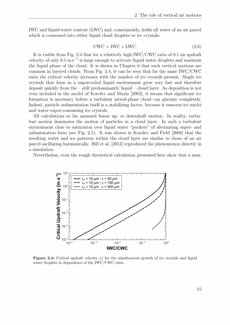
2. The role of vertical air motions
IWC and liquid-water content (LWC) and, consequently, holds all water of an air parcelwhich is consensed into either liquid cloud droplets or ice crystals:
CWC = IWC + LWC. (2.6)
It is visible from Fig. 2.4 that for a relatively high IWC/CWC ratio of 0.1 an updraftvelocity of only 0.1 m s−1 is large enough to activate liquid water droplets and maintainthe liquid phase of the cloud. It is shown in Chapter 6 that such vertical motions arecommon in layered clouds. From Fig. 2.4, it can be seen that for the same IWC/CWCratio the critical velocity increases with the number of ice crystals present. Single icecrystals that form in a supercooled liquid environment grow very fast and thereforedeposit quickly from the – still predominantly liquid – cloud layer. As deposition is noteven included in the model of Korolev and Mazin [2003], it means that significant iceformation is necessary before a turbulent mixed-phase cloud can glaciate completely.Indeed, particle sedimentation itself is a stabilizing factor, because it removes ice nucleiand water-vapor-consuming ice crystals.
All calculations so far assumed linear up- or downdraft motion. In reality, turbu-lent motion dominates the motion of particles in a cloud layer. In such a turbulentenvironment close to saturation over liquid water “pockets” of alternating super- andsubsaturation form (see Fig. 2.5). It was shown in Korolev and Field [2008] that theresulting water and ice patterns within the cloud layer are similar to those of an airparcel oscillating harmonically. Hill et al. [2013] reproduced the phenomenon directly ina simulation.
Nevertheless, even the rough theoretical calculation presented here show that a mea-
Crit
ical
Upd
raft
Velo
city
[m s
-1]
10−4
10−3
10−2
10−1
100
101
IWC/CWC10−4 10−3 10−2 10−1 100
rw = 10 µm ; ri = 50 µmrw = 10 µm ; ri = 100 µmrw = 10 µm ; ri = 500 µm
Figure 2.4: Critical updraft velocity u∗z for the simultaneous growth of ice crystals and liquidwater droplets in dependence of the IWC/CWC ratio.
15

Subsaturation
Supersaturation
Air movement
Hei
ght
Horizontal Distance
Figure 2.5: In a turbulent environment large eddies break down into smaller ones creating adistribution of super- and subsaturated regions inside the turbulent cloud layer.
surement uncertainty considerably lower than 1 m s−1 is required to capture the verticalair motion at cloud base. The temporal resolution of the measurements has to be highenough to record the breakdown of the turbulent eddies. At the same time, the mea-surements have to resolve IWC/CWC ratios lower than 10−3. Therefore, in Chapters 3,4 and 6, the ability of lidars and radars to measure and quantify IWC and LWC isexplored. In Chapter 5 the velocity resolution of the employed lidar and radar systemsis analyzed, together with their ability to probe turbulence.
2.4 Connecting observations with simulationsThe influence of turbulence on mixed-phase layered clouds has been subject of manytheoretical [Korolev and Mazin, 2003; Field et al., 2013] and modeling studies [Hillet al., 2013] recently. In the framework of the UDINE project own simulations havebeen carried out at TROPOS by Martin Simmel [Simmel et al., 2014]. In Fig. 2.6 anexample case study of a mixed-phase layered cloud is depicted. It assumes differentvertical-velocity distributions in a humid layer about 4000 m above the surface. Allother environmental constraints like temperature, humidity and aerosol load are basedon the measurement of a mixed-phase cloud layer over Leipzig on 17 September 2011.
It can be seen from Fig. 2.6 that the vertical velocity distribution has decisive impacton the evolution of the cloud layer. Stronger vertical motions lead to the condensation ofmore water vapor and thus enhance ice formation and deposition. The resulting IWC inthe virga below cloud top layer is on the order of 10−8 kg m−3 and varies by a factor of 2for a vertical-velocity standard distribution σv between 0.3 and 0.7 m s−1. Ice productionis so weak that loss of water and IN scavenging due to ice deposition has no visible effecton the time scale of the simulation. Given sustained turbulent motions, such a cloud
16

2. The role of vertical air motions
a) σv = 0.3 m s−1
Hei
ght [
m]
Ice
Wat
er C
onte
nt [k
g m⁻³
]
Time [min]
v = 0.3 m s⁻¹
b) σv = 0.5 m s−1
Hei
ght [
m]
Ice
Wat
er C
onte
nt [k
g m⁻³
]
Time [min]
v = 0.5 m s⁻¹
c) σv = 0.7 m s−1
Hei
ght [
m]
Ice
Wat
er C
onte
nt [k
g m⁻³
]
Time [min]
v = 0.7 m s⁻¹
Figure 2.6: Simulation of heterogeneous ice formation in a liquid layer for different vertical-velocity standard deviations σv [Martin Simmel, personal communication]. The measured standarddeviation of vertical velocity at cloud base was σv = 0.44 m s−1. An initial updraft is used togenerate cloud droplets in the air parcel, then it is oscillating harmonically. A random vertical-velocity pattern is added with the amplitude of the harmonic oscillation. A similar approachwas chosen by Korolev and Field [2008]. The increased ice production in the initial updraft at(b) compared with (a) and (c) may be an artifact of the simulation. 20 min after start of thesimulation, the amount of ice production increases with increasing σv from 1× 10⁻⁸ kg m−3 (a) to2.5× 10−8 kg m−3 (c). Contour lines of LWC have a constant spacing of 3× 10⁻⁵ kg m−3 and alsostart at this value. A more detailed evaluation of the real cloud case is carried out in Section 6.2.
17

layer will be stable over hours.
2.5 Arising questionsThe theoretical considerations discussed in this chapter ultimately lead to different ques-tions to be answered:
• What ratios between liquid water and ice can be observed within mixed-phaselayered clouds with respect to mass and number concentration?
• What are the statistical properties of the vertical air motions within these clouds?
• What is the critical ratio between ice and water at which the ice dominates themicrophysics within the mixed-phase cloud layer and the cloud will glaciate com-pletely?
These questions cannot be answered by measurements alone, but also require cloudmodeling and laboratory work. An experiment carried out in nature can provide mod-elers both input parameters and values to test the results. In Section 2.4 measuredvertical-wind velocity was used as input and the IWC as a reference. Such end-to-endsimulations can only succeed, if the input and the reference data are quality-assuredand treated to be free of artifacts. In this work, ways towards precise measurementsof vertical-wind velocity at cloud base will be shown in Chapter 5, involving Dopplerlidar, cloud radar and wind profiler systems. The main benefit of this combination isthe simultaneous measurement at different target sizes ranging from aerosol particles torain droplets. The synergy between the single measurement systems can be very high,but data of all instruments have first to be brought down to a common time and heightgrid. Chapter 4 describes such a combined data processing. Especially the cloud radardelivers much more information than only velocity measurements. From its signals onecan, e.g., obtain the IWC (see Chapter 6). In future, it may be even possible to derivethe ice crystal number concentrations (see Chapter 7). Bringing all these quantitativemeasurements together one will be able to approach the questions above on a solid basis.
18

3 Lidar and radar synergy. Part I:Signal strength
Combining lidars and radars is useful but also very challenging because of their greattechnical differences. The most prominent example may be that the signal sensitivity fora liquid water droplet with diameter D is proportional to D2 for lidar and D6 for radar.Such differences must be kept in mind during the evaluation of combined measurements.In this chapter, differences and similarities of both remote-sensing systems are exploredon a theoretical basis [Wandinger, 2004; Peters and Gorsdorf, 2010]. It is shown inSection 3.1, what assumptions are necessary to describe the measurements of lidars andradars with a common equation. The ability of lidar and radar to probe the propertiesof particles in mixed-phase cloud layers is examined in Section 3.2. In Section 3.2.4the terminal fall velocity of cloud droplets and ice crystals is analyzed to support theinterpretation of Doppler lidar and cloud radar measurements.
From the physical viewpoint, lidars and radars are very similar. Both emit pulsesof electromagnetic radiation through an aperture and detect the fraction of radiationscattered back. For the TROPOS Multiwavelength Atmospheric Raman Lidar for Tem-perature, Humidity, and Aerosol Profiling (MARTHA) [Mattis et al., 2004] and theMIRA-35 cloud radar of LACROS [Bauer-Pfundstein and Gorsdorf, 2007] surprisingsimilarities prevail for the emitter/receiver aperture sizes (dr ≈ 1 m) and the averageemitted power (P ≈ 30 W). The main difference between the two systems is the wave-length of the emitted radiation, which is 355 to 1064 nm for the lidar and 8.5 mm forthe radar. To find a common description for lidar and radar, monochromatic systemsoperating at wavelengths λL/R (in the following, indices L and R stand for “lidar” and“radar”, respectively) are assumed.
3.1 Description of lidar and radar backscattering
3.1.1 Generalized equation for active remote sensingElectromagnetic radiation is diffracted by any aperture it is sent through [Goodman,2005b]. The resulting diffraction pattern is characteristic for both emission and receptionof electromagnetic radiation through that aperture. Close to the aperture, in the so-called Fresnel zone, this pattern has range and angular dependence. More far away, inthe so-called Fraunhofer zone, only angular dependence remains. The distance from theaperture to the end of the Fresnel zone can be estimated by rFZ = 2d2
r/λ, where dr is thediameter of the emitter aperture. rFZ is about 250 m for the MIRA-35 cloud radar and
19

Radar
Pulse VolumeVp(r)
Lidar
Pulse AreaAi(r)
Folded Pulse Length lf
Receiving Telescope Field of View
Radar Antenna Pattern
LidarOverlap Region
EmissionReception
Lidar Blind Zone
Figure 3.1: Comparison of the characteristics of radar (left) and lidar (right). The angular-dependent radar antenna pattern is depicted schematically. At φ/2 from emission direction, thesensitivity of the antenna has dropped by 3 dB. Because the same antenna is used for emission andreception, the total dampening is 6 dB and φ is defined as the opening angle of pulse propagation.The first diffraction minimum is at θ/2 from emission direction. θ then contains the whole mainlobe of the emitted radiation. In this view, a lidar with separated biaxial emitter and receivertelescope is depicted (e.g., PollyXT) leading to a a blind zone and a region of incomplete overlap.
more than 300 km for the MARTHA lidar. For a circular aperture, the angular width ofthe main lobe (inside the first diffraction minimum) is θ = 2.44λ/dr . Within this mainlobe, about 84% of the diffracted power are contained. θ is approximately 1.22 for thecloud radar and 7.6× 10⁻⁵ for the MARTHA lidar. Fig. 3.1 illustrates the differentpropagation characteristics for lidars and radars.
For lidars, the receiving telescope can be designed in such a way that its field ofview is considerably bigger than the divergence of the propagating laser pulse. If this isthe case, any angular dependence of the receiver can be neglected, as long as the laserpulse has left the overlap zone (see Fig. 3.1). For monostatic radars like the MIRA-35,radiation is always emitted into and received from the half-space. The same antenna isused for emission and reception, so the field of view of the antenna matches its emissioncharacteristics. At φ/2 from emission direction, the received signal has decreased from0 dB (beam center) to −6 dB. For simplicity, it is assumed that the radar only emitsradiation within the opening angle φ [Peters and Gorsdorf, 2010]. The volume of oneradar pulse is then defined as
Vp,R(r)!
=lπ(φr)2
4, (3.1)
20

3. Signal strength of lidar and radar
with pulse length l = clτ (cl the velocity of light and τ the temporal pulse length). Theso defined pulse volume has a nearly cylindrical shape and is proportional to r2. Forthe MIRA-35 cloud radar of LACROS, φ is about 0.5 which corresponds to a pulsediameter of approximately 10 m in a range of 1 km. The emitted power inside this(theoretical) pulse volume has to be determined experimentally. This calibration is onemajor issue of cloud radar research [Hogan et al., 2003]. It has to be kept in mind thatthe defined signal drop to −6 dB at φ/2 is only a factor of about 0.25. Hence, in anatmospheric scene with high spatial variabilities, the signal will be mixed with signalsfrom adjacent scatterers from outside the defined pulse volume Vp,R(r). This problem isespecially relevant for AC clouds. In this case, the radar can only deliver averaged cloudproperties. The signal of a lidar is received from a much more restricted volume.
With the assumptions made above, it is possible to formulate a common equation forthe signal received by lidar and radar. The power Pc(r) collected by a receiver withaperture (telescope mirror) area At from an atmospheric volume at range r scatteringback electromagnetic radiation of power PΩ into the solid angle Ω is
Pc(r) =
∫Ω(r)
PΩ(r)T (r) dΩ. (3.2)
r is the range between the aperture and the illuminated volume, Ω is the solid angle underwhich the aperture appears from distance r and T (r) is the transmission term whichdescribes the range-dependent signal extinction between the emitter and distance r. Ina remote-sensing application, PΩ(r) is proportional to the intensity Ii of the radiationincident on the observed volume and the total scattering cross section SΩ of the observedvolume. Hence, the expression of Pc(r) further expands to
Pc(r) =
∫Ω(r)
SΩ(r)Ii(r)T (r) dΩ =
∫Ω(r)
SΩ(r)P0
Ai(r)T 2(r) dΩ. (3.3)
P0 is the power of the emitted pulse and Ai(r) is the mean cross section of the illuminatedvolume (see Fig. 3.1). The scattering properties within the illuminated volume Vi(r) canbe expressed as
SΩ = B(r)Vi(r), (3.4)
if a backscattering geometry is assumed (see Fig. 3.1). B(r) describes, how the objectswithin Vi scatter back radiation into the solid angle Ω. If the aperture size At is smallagainst r2, Eq. (3.3) becomes
Pc(r) = P0B(r)Vi(r)T
2(r)
Ai(r)
Atr2. (3.5)
The receiver may actually not be able to completely see the illuminated volume Vi.This can be the case, e.g., in the overlap zone of the lidar, where the laser pulse is stilloutside the field of view of the telescope (Fig. 3.1). Thus, the illuminated volume Vi(r)
21

is replaced by Ailf multiplied by a function O(r):
Pc(r) = P0O(r)B(r)Ai(r)lfT
2(r)
Ai(r)
Atr2. (3.6)
Here lf = clτ/2 is the folded pulse length. In this way, Eq. (3.6) reduces to the general-ized active-remote-sensing equation
Pc(r) = P0lfAtO(r)B(r)T 2(r)1
r2. (3.7)
The meaning of the single terms is explained in the next section. Equation (3.7) describesthe power that reaches the receiving telescope. To derive the power that actually reachesthe receiver, the efficiency of the receiver unit has to be taken into account. It isusually collected in a system constant CR,L, including also P0, lf and At and determinedexperimentally.
3.1.2 Detailed description of all terms3.1.2.1 Pulse power P0 and effective pulse length lp
For both lidar and radar, a temporally rectangular pulse is assumed with the meanenergy P0. The folded length of the pulses is lf = clτ/2, which is half of the physicalpulse length due to folding of the pulse in backscatter observations.
3.1.2.2 Receiver aperture At
The aperture area of the lidar telescope corresponds to the effective aperture of the radarantenna. The latter is defined as Ae = λ2
R/(4φ2) and has the unit m2. For the MIRA-35
cloud radar of LACROS Ae = 0.23 m2. This value compares to the MARTHA lidar with0.5 m2 and the PollyXT lidar with 0.07 m2 telescope area.
3.1.2.3 Overlap function O(r)
The receiving telescope of a lidar does usually not completely see an emitted laser pulseup to a certain height. The overlap function O(r) describes the resulting influence onthe received signal. Depending on the system, it approaches 1 within the first fewhundred (PollyXT) or thousand meters (MARTHA). Doppler lidars like WiLi alwayshave a perfect geometric overlap, because the telescope is transmitter and receiver atonce (transceiver). Regardless, the introduction of a function like O(r) makes sense forWiLi, because in the lowest 500 m the receiver of the atmospheric signal shows non-lineareffects by overload from straylight during pulse emission and defocus of the atmosphericsignal.
The radar receiver/emitter system shows similar behavior. Close to the emitter, thesignal is received at full strength, but may not be useful for atmospheric measurements.O(r) cannot be described easily analytically but it approaches 1 at the end of the Fresnel
22

3. Signal strength of lidar and radar
zone of the radar. In a mathematical sense, O(r) can also be useful to remind thatEq. (3.7) is not valid for r → 0, due to the assumption of small solid angles.
3.1.2.4 Volume backscatter properties B(r)
B(r) holds the backscatter properties of the particles within the pulse volume and is themain measurement goal. In general, it holds the volume-averaged backscatter properties,i.e.,
B(r) =∑n
∫ ∞0
Nn(r,D)∂sn(r,D)
∂Ω
∣∣∣∣180
dD!
=∑n
∫ ∞0
Nn(r,D)sn,180(r,D) dD, (3.8)
with the number concentration Nn(r) of the n-th particle type in the scattering volumeand the particles’ differential backscattering cross section sn,180 .
The ice and water particles observed in the context of this work are in the size range of10 µm to 1 mm. The millimeter waves of the radar will, therefore, experience Rayleighscattering and
sR180 =1
4π
π5
λ4K2w,iD
6. (3.9)
Kw,i is the material-dependent dielectric factor at 35 GHz, which is K2w = 0.93 for liquid
water and K2i = 0.174 for ice. The volume-equivalent diameter D is connected with the
mass mp of a particle:
D =
(6
πρw,imp
)1/3
, (3.10)
where ρw,i is the density of liquid water or ice. D matches the geometric diameter forspherical particles. A mixture of liquid water droplets and one type of ice crystals inthe scattering volume leads to
BR(r) =η(r)
4π=
1
4π
π5
λ4R
(K2w
∫ ∞0
Nw(r,D)D6 dD +K2i
∫ ∞0
Ni(r,D)D6 dD
)=
1
4π
π5
λ4R
Z(r), (3.11)
with the radar scattering cross section η(r) and the particle number concentrations Nw,i
for liquid water (w) and ice particles (i). Z(r) is the radar reflectivity factor
Z(r) = K2w
∫ ∞0
Nw(r,D)D6 dD +K2i
∫ ∞0
Ni(r,D)D6 dD. (3.12)
The physical unit of Z is 1 m6 m−3 in this notation. Z is usually normalized by thesignal Z0 = 0.93× 0.0016 m6 m−3, which is the radar reflectivity factor of a volume filledwith droplets with D = 1 mm and N = 1 m−3. Z is usually depicted on a decibel scaleas ZdBZ = 10 log(Z/Z0). The corresponding unit is denoted dBZ.
The backscatter signals for lidars can be calculated easily in the limits of geometrical
23

optics. In this case,
sL180 =2ApL. (3.13)
Ap is the particle area projected to the fall direction, L is the extinction-to-backscatterratio (lidar ratio). In the visible wavelength range, the lidar ratio Lw ≈ 18 sr for liquiddroplets and Li = 20...30 sr for ice particles. The lidar ratio of ice crystals can bedetermined with numerical methods [e.g., Macke et al., 1996]. Taking into accountEq. (3.13), the backscatter term for lidar in Eq. (3.7) becomes
BL(r) = β(r) =∑n
∫ ∞0
Nn(r,D)2Ap,n(D)
LndD. (3.14)
β is called the volume backscatter coefficient. For lidars in the optical wavelengthrange, molecular scattering adds to BL(r), but this additional scattering can be removed[Ansmann et al., 1990]. For both lidar and radar, the function B(r) can depend on morecharacteristic parameters. For Doppler lidars and radars, e.g., the particle velocity vcan be included and particle number concentration N(r, v) can be defined. The receivedpower Pc(r) then becomes a two-dimensional function Pc(r, v), which is represented inheight-resolved Doppler spectra. The treatment of such spectra is discussed in Chapter 5,cloud-radar spectra are subject of analysis in Chapter 7.
3.1.2.5 Transmission term T(r)
The transmission term T (r) defines the extinction of electromagnetic radiation by ab-sorption and scattering. For monochromatic lidars and radars, the extinction on theway to the target is the same as on the way back. Thus, the Lambert-Beer law describesthe transmission as
T (r) = exp
(−2
∫ r
0
α(r′) dr′), (3.15)
with α being the electromagnetic extinction coefficient at a certain range. For lidars,the extinction coefficient is connected with the backscatter coefficient via the extinction-to-backscatter ratio L = α/β (lidar ratio). Assuming a homogeneous particle popula-tion, the extinction can be estimated for known particle types. With Raman lidars likeMARTHA this quantity can be derived together with the backscatter coefficient. Stan-dard methods to derive β(r) and α(r) from lidar measurements are given by Klett [1981](elastic backscatter lidar) and Ansmann et al. [1990] (Raman lidar).
In the layered clouds, which are treated in this work, particle extinction is very low fora 35-GHz radar. At this high radar frequency also gas attenuation in the free atmospherecan play a role. This attenuation depends, e.g., on the water vapor path betweenthe radar and the observation volume and is usually smaller than 1 dB in the wholetroposphere for observations at Leipzig. Radar attenuation is therefore not furtherconsidered in the scope of this work, if radar data is evaluated manually. All valuesderived with the help of Cloudnet [Illingworth et al., 2007] (introduced in the nextchapter) are automatically corrected for gas attenuation.
24

3. Signal strength of lidar and radar
3.2 Detection of spherical and non-spherical particleswith lidar and radar
Cloud droplets and ice crystals can both be detected with lidar and radar. For studies ofheterogeneous freezing in the atmosphere, it is important to know the detection limits ofthe different systems. The main difference between lidar and radar is the dependence ofthe backscatter term BL,R in Eq. (3.7) on the particle properties. For lidar, mostly geo-metric scattering is involved, so that the particle backscatter coefficient is proportionalto Ap. The radar operates in the Rayleigh scattering regime and the radar reflectivityfactors of liquid droplets or ice crystals are proportional to D6 or to the square of particlemass m2
p.
3.2.1 Linear depolarization ratioEquation (3.12) shows that the meaning of Z is ambiguous, if no additional informationabout phase, shape and spectral distribution of the scattering particles is available.Pure detection of particles is, therefore, not sufficient. The polarization state of theelectromagnetic radiation received from the target volume can be used to decide between(spherical) water droplets and non-spherical targets like ice crystals. The latter inducea depolarization on both lidar and radar signals. To measure this polarized radiation,the backscattered signal is received in two channels simultaneously, with perpendicularpolarization sensitivity. One way to calculate the linear depolarization ratio δ is todivide the signals received in the perpendicular and the parallel channel and to derivethe depolarization ratio δ = P⊥/P‖. δ can be about 0.5 for lidars, when observingice crystals [Mishchenko and Sassen, 1998; Sassen, 2004]. In contrast, δ rarely exceeds0.01 or 10 log(0.01) dB = −20 dB for 35-GHz radars, where this measurement quantityis usually designated LDR (for linear depolarization ratio) and measured in dezibel[Reinking et al., 1997; Matrosov et al., 2012]. The identification of liquid water and iceparticles in layered clouds with the help of the depolarization ratio is further treated inChapter 4.
3.2.2 Area and mass parameterizationsArea Ap and mass mp of ice and water particles have to be known in order to estimatetheir backscatter properties. Especially for ice crystals this estimation is difficult, be-cause their geometry is complex and changes significantly during growth. Mandelbrot[1982] showed that the shapes of some naturally formed objects, like ice crystals, can bedescribed by fractal geometry over large size ranges. Mitchell [1996] used this idea todescribe area Ap and mass mp of ice particles by fractal power-laws, depending on theice particles’ maximum diameter Dm (the diameter encircling the area projected to flow
25

a)
M
Particle Maximum Diameter [µm]
Par
ticl
e A
rea
[m²]
b)
Particle Maximum Diameter [µm]
Par
ticl
e M
ass
[kg
]
M
Figure 3.2: Selected parameterizations of particle area Ap (a) and particle mass mp (b) fromMitchell [1996], depending only on the particles’ maximum diameter Dm. All values are shownin their ranges of validity. Hexagonal plates are parameterized unsteadily at Dm = 100 µm. Forhexagonal columns the continuation is steady at this diameter, but bends sharply.
26

3. Signal strength of lidar and radar
direction) in the form
Ap(Dm) = aDbm, (3.16)
mp(Dm) = cDdm. (3.17)
The coefficients a, b, c and d can be determined experimentally. Mitchell [1996] liststheir numerical values and ranges of validity for a broad spectrum of ice crystal species.The maximum diameter Dm does not have a direct influence on the calculation of signalstrength. It is only a characteristic length to connect the area and mass parameteriza-tions. Figure 3.2 shows some parameterizations from Mitchell [1996] for particle speciesthat are used in this work. For hexagonal columns b = 2.0...1.4 (from small to largeparticles) and c = 2.9...1.74. For aggregates of side planes b = 1.88 and c = 2.2.
3.2.3 Particle detection thresholdsFor a simplified monodisperse size distribution of spherical particles, the critical particlenumber concentration can be calculated, which is needed to surpass the detection limitsof lidar or radar. The minimum detectable backscatter signals βmin and ηmin are dividedby the single-particle returns from Eqs. (3.9) and (3.13), so that the critical numberconcentrations for radar and lidar can be defined as
NLcrit =
βmin
sL180=
2Lβmin
Ap(3.18)
and
NRcrit =
ηmin
4πsR180=
(πρw,i)2Zmin
18K2w,im
2p
. (3.19)
The particle diameter Des, for which lidar and radar are equally sensitive, can be derived
by demanding NRcrit
!= NL
crit and inserting Eqs. (3.16) and (3.17), so that
Des =
(a(πρw,i)
2
18c2K2w,iLw,i
Zmin
βmin
) 12d−b
. (3.20)
For liquid water droplets a = π/4, b = 2, c = ρwπ/6 and d = 3 and Eq. (3.20) reducesto
Des =
(π
2K2wLw
Zmin
βmin
) 14
. (3.21)
Below Des, the lidar can detect particles at lower number concentrations than the radar,above vice versa. Figure 3.3 presents the trend of Ncrit(Dm) over the range 1 µm < Dm <3 mm for these minimum detectable signals. It shows that lidar and radar complementeach other in the size range of very small and very large particles. From Fig. 3.3 itbecomes obvious that the MIRA-35 cloud radar is in principle capable of detecting ACclouds, but it will largely miss activation of small droplets at the cloud base whereD ≈ 2..10 µm (D and Dm are equivalent for small cloud droplets). For this purpose, the
27

Ice Virgae
Rain
CumulusC
riti
cal N
um
ber
Co
nce
ntr
atio
n [
m⁻³
]
10−5
100
105
1010
Particle Maximum Diameter [µm]100 101 102 103
Water Droplets (Radar, Zmin = -50 dBZ)Water Droplets (Lidar, βmin = 1 Mm⁻¹sr ⁻¹)Ice Columns (Radar, Zmin = -50 dBZ)Ice Columns (Radar, Zmin = -30 dBZ)Ice Columns (Lidar, βmin = 1 Mm⁻¹sr ⁻¹)
Drizzle
Altocumulus
Figure 3.3: The critical particle number concentration Ncrit is shown for radar (solid lines)and lidar (dashed lines). Any monodisperse particle concentration lower than Ncrit does notproduce a detectable signal for the corresponding system. Assumptions on minimum signals wereZmin = −50 dBZ and βmin = 1 Mm−1 sr−1. Lidar ratios were assumed to be Lw = 18 sr (waterdroplets) and Li = 25 sr (ice crystals). Therefore, Li is at least 20% accurate for all particles. Bluecurves indicate water droplets. The line for hexagonal columns (bright red curves) is assembledfrom different parameterizations in the appropriate size ranges from 30 µm to 600 µm. Above, theparameters of rimed long columns are applied. It is visible that for small maximum diameters, thecurve of hexagonal columns approaches the theoretical curve of spherical particles (solid blue line).In the background, expected ranges of droplet and ice-particle number concentrations in clouds,virgae and rain are shown.
lidar is better suited. On the other hand, the radar can detect columnar ice particleswith Dm ≈ 300 µm, if their number concentration is only 1 m−3. At the same maximumdiameter, the critical number concentration for lidars is about two orders of magnitudelarger.
In the mid-troposphere, the MIRA-35 cloud radar is designed to detect Zmin ≈−50 dBZ. In Chapter 6 the minimum detectable backscatter signal of PollyXT andMARTHA lidars is statistically determined to be βmin = 1 Mm−1 sr−1 for an integrationtime of 30 s. These values yield Des = 31 µm for liquid water droplets. In the case ofcolumnar ice particles and the same signal thresholds Des = 57 µm. It is visible fromFig. 3.3 that for small Dm the curves of hexagonal columns run parallel to those ofspherical water droplets.
Pure particle detection alone is not the only goal of remote sensing, the particle type
28

3. Signal strength of lidar and radar
is also of great interest. Depolarization can help to unambiguously decide between liquidwater and ice particles. However, particle classification by depolarization needs highersignal strengths than particle detection alone. If Zmin = −50 dBZ is assumed and anobserved volume is filled with ice crystals, which induce a depolarization δ ≈ −20 dB, thesignal received from this volume has to be larger than −30 dBZ, until a depolarizationcan be detected. The dark red curves in Fig. 3.3 show the critical number concentrations,obtained for the signal thresholds Zmin = −30 dBZ and βmin = 1 Mm−1 sr−1, shifting Des
to about 338 µm. Lidars measure the depolarization more easily, because with δ ≈ 0.5the signal received in the depolarization channel is on the same order of magnitude asthe total signal. In Section 4.5 of the next chapter, combined particle classification bylidar and radar is treated in more detail.
3.2.4 Terminal fall velocitiesThe terminal fall velocity of ice and water particles has to be taken into account carefully,when dealing with vertical-velocity measurements from Doppler lidars and cloud radars.On the one hand, falling particles can disturb and offset measurements. On the otherhand, the terminal fall velocity yields information about particle size and shape. Thelatter will be exploited in Chapter 7 to derive number concentrations of falling particlesfrom cloud radar spectra. In the following, vertical velocities derived from moving cloudparticles are denoted v, in contrast to the vertical air velocity uz introduced before.
According to Heymsfield and Westbrook [2010] the calculation of a particle’s terminalfall velocity is a three-step process. First, the so-called Best number X∗ is calculated,which contains the basic information about the particle (mass mp and area ratio Ar =Ap/(
π4D2m) and the surrounding air (density ρair, dynamic viscosity of air ηair, acceleration
of gravity g):
X∗ =8mpgρair
πηairA(1−k)r
. (3.22)
k is a dimensionless empiric parameter introduced to achieve better agreement withlaboratory studies. Heymsfield and Westbrook [2010] found that the Reynolds numbersRe fit best the laboratory measurements, if k = 0.5 and
Re =γ2
0
4
(1 +4√X∗
γ20
√γ1
)0.5
− 1
2
, (3.23)
with γ0 = 8.0 and γ1 = 0.35. The terminal fall velocity is then computed by
vt =ηairRe
ρairDm
. (3.24)
In Fig. 3.4 the terminal fall velocities are calculated for different particle species, assum-ing pressure p = 650 hPa and temperature T = 260 K.
29

M
Particle Maximum Diameter [µm]
Term
inal
Fal
l Vel
oci
ty [
m s⁻¹
]
Figure 3.4: Terminal fall velocities of different particle species calculated with the method ofHeymsfield and Westbrook [2010] for T = 260 K and p = 650 hPa. The gap in the curve forhexagonal plates originates from the unsteadiness in the area parameterization described in Fig. 3.2.
30

4 TROPOS remote-sensing facility forsimultaneous profiling of aerosols,clouds and meteorologicalparameters
Investigation of cloud processes involves a huge variety of length scales [Bodenschatzet al., 2010], ranging from aerosol particles of some nanometer in diameter to cloudfields, hundreds of kilometers wide. This wide scale range poses a great challenge toremote-sensing methods, because the sensitivity of any instrument is restricted to a cer-tain target size range. Only a combination of different measurement systems can map allfacets of a cloud system. The Leipzig Aerosol and Cloud Remote Observations System(LACROS) is a set of remote-sensing and in-situ measurement systems of TROPOS,dedicated to the continuous observation of clouds and aerosols. The integration intoobservation networks like Cloudnet [Illingworth et al., 2007], EARLINET (EuropeanAerosol Research LIdar NETwork) and AERONET (AErosol RObotic NETwork) opensa great diversity of possible scientific applications. LACROS combines the strengths oflidar, radar and radiometer techniques and employs auxiliary systems like a meteorologi-cal ground station and an advanced all-sky imager. The span of observation wavelengthsranges from 355 nm (Raman lidar) to centimeters (cloud radar and microwave radiome-ter).
4.1 Instrument overviewA schematic overview about all instruments gathered around the TROPOS main buildingis given in Fig. 4.1. It has been one major goal of this work to bring together themeasurements recorded by the different systems.
For active vertical profiling of the atmosphere different active remote-sensing instru-ments are employed:
• PollyXT Raman/polarization lidar,
• WiLi coherent Doppler wind lidar,
• MIRA-35 cloud radar,
• CHM 15kx ceilometer.
31
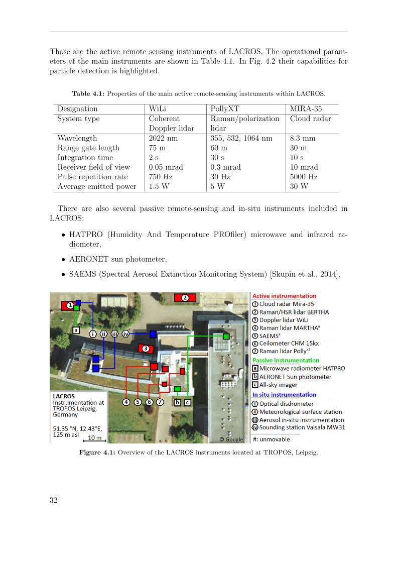
Those are the active remote sensing instruments of LACROS. The operational param-eters of the main instruments are shown in Table 4.1. In Fig. 4.2 their capabilities forparticle detection is highlighted.
Table 4.1: Properties of the main active remote-sensing instruments within LACROS.
Designation WiLi PollyXT MIRA-35System type Coherent
Doppler lidarRaman/polarizationlidar
Cloud radar
Wavelength 2022 nm 355, 532, 1064 nm 8.3 mmRange gate length 75 m 60 m 30 mIntegration time 2 s 30 s 10 sReceiver field of view 0.05 mrad 0.3 mrad 10 mradPulse repetition rate 750 Hz 30 Hz 5000 HzAverage emitted power 1.5 W 5 W 30 W
There are also several passive remote-sensing and in-situ instruments included inLACROS:
• HATPRO (Humidity And Temperature PROfiler) microwave and infrared ra-diometer,
• AERONET sun photometer,
• SAEMS (Spectral Aerosol Extinction Monitoring System) [Skupin et al., 2014],
Figure 4.1: Overview of the LACROS instruments located at TROPOS, Leipzig.
32

4. TROPOS remote-sensing facility
• Photographic all-sky imager (vertically looking camera with 180 fisheye lens),
• Disdrometer for sensing size and fall speed of raindrops.
4.2 Measurement exampleFigure 4.3 shows an example of a LACROS measurement on 30 May 2012 around 18:00UTC. An AC cloud approached Leipzig from northwest with a horizontal wind speedof 16 m s−1. The cloud-camera image is depicted together with the Cloudnet targetclassification product. The lidars show clear signals at about 3200 m height, whilethe radar only partially senses the liquid cloud top. However, the radar senses fallingparticles nearly everywhere in the virga, while the lidar only detects a short precipitationevent at 18:30 UTC.
In Fig. 4.4, the vertical velocity measurement from a timespan of only about 2 min
DopplerLidar
RamanLidar
CloudRadar
Radio-meter
Melting Layer (T = 0 °C)
Falling Ice Crystals
Drizzle/Rain
Mid-Level Cloud
aerosols/pollenoriented icecloud base
aerosols/pollenice crystalscloud base
insects/pollencloud topsbig ice crystalsbig droplets
all liquid water
Systems
ObservationCapabilities
DetectedUndetected
Figure 4.2: Comparison of the different particle detection capabilities of four LACROS systems.Detected particles are depicted in color, others are left blank. The lidars detect the particles atcloud base and some of the falling ice crystals. The PollyXT is powerful enough to detect all kindsof particles, the Doppler lidar has a much weaker emitter and only detects ice particles if theyare oriented parallel to the ground. The cloud radar can detect the falling particles very well, butcannot detect the small, freshly activated particles at cloud base. The microwave radiometer givesan integral value of liquid water path and total atmospheric water vapor content. It is visible thatthe four systems complement each other so that all particles types are resolved.
33

advection vector (16 m/s)
TROPOS All-Sky Imager 2012-05-30 17:53 UTC
Single-Measurement Paths of
Doppler Lidar WiLi (2 s)Ceilometer/PollyXT/Martha (30 s)Cloud Radar MIRA-35 (10 s)CPR Radar on CloudSat (1 shot)
Range-C
orr
ect
ed S
ignal [a
.u.]
Vert
ical Velo
city
Radar
Refleci
vit
y F
act
or
[dB
Z]
WiLi Doppler Lidar Cloud Radar
Cloudnet ClassificationCeilometer
Figure 4.3: Photo from the all-sky imager of an altocumulus cloud depicted together with timeseries of lidar backscatter (ceilometer), vertical velocity (WiLi), radar reflectivity factor (MIRA-35cloud radar) and the Cloudnet target classification product. The red line indicates the time of thephoto. In the magnified portion of the photo the size of the observation areas of the LACROSremote sensing instruments and, additionally, the footprint of the Cloud Profiling Radar (CPR)on the CloudSat Satellite are shown.
34

4. TROPOS remote-sensing facility
0 s 30 sa)
b)
c)
WiL
i V
ert
ical V
elo
cit
y [
m s
⁻¹]
Time [UTC]
Figure 4.4: Comparison between vertical velocity measured by the Doppler lidar and photographsfrom the all-sky imager (±15 around zenith) taken simultaneously. Time of the photographs is±1 min around 17:54 UTC (like in Fig. 4.3). Panel a) shows two cloud-camera images taken 30 sapart. In this time period the change in the image is governed by the movement of the total cloudfield, changes in the visible cloud pattern itself are negligible. By overlaying the correspondingvertical-velocity measurements from WiLi (for velocity scale and height see (c)) at cloud base, onecan see cloud formation in the updraft regions (yellow) and cloud evaporation where downdraftsprevail (green). Panel b) shows a series of images and panel c) the simultaneously recordedDoppler-lidar measurements over about 2 min.
is depicted. It shows that updrafts (yellow and red color) are mainly connected withthe visible parts of the cloud, while downdrafts (green and blue) are mainly seen wherethere are visible gaps in the broken cloud pattern.
4.3 Measurement strategy for the UDINE campaign atLeipzig (2010–2013)
LACROS has been run operationally since August 2011. It was a goal of the UDINEproject to integrate Doppler Wind Lidar “WiLi”, developed at TROPOS from 2002 to2005, into the measurement platform LACROS. To enable unattended long-durationmeasurements with WiLi, remote supervision and control software was developed and
35

installed together with additional hardware. WiLi was set to measure vertically with hightemporal resolution (2 s per profile). Simultaneously, Cloudnet derived microphysicalproperties like LWC and IWC with ceilometer, cloud radar and microwave radiometer.From the PollyXT lidar mainly the polarization information has been used to decidewhether falling particles are ice crystals or liquid water droplets. To get more insightinto the nature of falling particles, four times an hour WiLi performed a 1 min long“rocking over the zenith” (ROZ) scan to search for specular reflections of oriented iceparticles in cloud virgae [Westbrook et al., 2010]. In this observation mode, the scanner istilted ±2 off-zenith in 0.25 steps. If in such a scan a drop in signal strength between thezenith and the off-zenith measurement is detected, the presence of oriented ice particlesis probable [Westbrook et al., 2010]. Such observations are used in the LACROS particleclassification scheme presented in Section 4.5.
During a ROZ scan an error is introduced into the vertical-velocity signal by theadvection speed, because the lidar does no longer point perpendicular to it. One canestimate the maximum error introduced into vertical-velocity measurements at cloudbase to sin(2)× 15 m s−1 = 0.52 ms−1 (assuming an advection speed of 15 m s−1). Thiserror affects about 6% of the measurement time of WiLi between 2011 and mid 2012.To keep this error out of the vertical-velocity statistics, off-zenith profiles are omittedwhen assembling the vertical-velocity statistics in Chapter 6.
4.4 LACROS data storage and processingUnder normal conditions, the amount of raw data recorded by the main instrumentsof the LACROS platform is on the order of 20 Gigabyte per day. Hence, significanteffort is necessary to process data and make it available to users. For that purpose,LACROS makes great use of the data collecting, sorting and processing abilities of theCloudnet software. The Cloudnet algorithms can handle a wide variety of remote-sensinginstruments, especially the MIRA-35 cloud radar. Recorded data is processed in near-real time, however, still depending on the availability of weather-model input data. Afterprocessing, data products are available on a fixed 30-s timegrid.
For immediate and direct access to the raw data of the LACROS instruments, theLACROS Research Data Application (LARDA) software suite has been developed. Itcan process and display data of any LACROS instrument on a common time and heightgrid, independent of the original time or height interval of the instruments. Large-scale meteorological information from the GDAS (Global Data Assimilation System)dataset can also be accessed. The LARDA software allows to quickly access, analyzeand compare data from the numerous LACROS systems. Interesting time-height sectionscan be marked as cases with a special visualization software. The cases are then storedin a simple database and can be recalled and processed later at any time. An overviewabout the software and the data processing chain is given in Fig. 4.5. An overview aboutthe usage of the data products is given in Fig. 4.6.
So far, one program for fast visualization and case selection (LARDA Explorer) andone program for advanced data evaluation (pyLARDA) have been developed in the
36

4. TROPOS remote-sensing facility
MIRA-35Cloud Radar
Ceilometer
Cloudnet Server
HATPRORadiometer
COSMOWeather Model
Doppler LidarWili
Deconvolution /Data-Reduction
PollyXT
Data ServerGDAS
Weather Model
raw data from remote- sensing instruments & GDAS weather modelCloudnet products:
- Ice Water Content- Liquid Water Content
PollyXT All-Sky Imager
LACROS Data Application (LARDA)
Data Visualization(LARDA Explorer)
Data Base
Data Processing(pyLARDA)
Cloud CaseManagement Data Products
Figure 4.5: Overview about the data acquisition chain.
Radar Reflectivity
Vertical Velocity
Linear DepolarizationRatio
Backscatter Coefficient
Vertical Velocity
Volume DepolarizationRatio
Radar Lidar
Ice-Water Content
Liquid-Water Content
Cloudnet
Pressure
Temperature
Models
Advection Speed
LACROS Target Classification(Separating Mixed-Phase and Liquid Clouds)
Vertical Velocity Statistics at Cloud Base and in Virga (Lidar & Radar)
Eddy Structure Analysis
Mixed-Phase Cloud Statistics / Quantification of Heterogenous Ice Formation
Mea
sur e
men
t V
alu
esD
ata
Pr o
du
cts
Figure 4.6: Overview about the data processing leading to the products used in this work.
37

Figure 4.7: Screenshot of the LARDA Explorer computer program. Desired time frame andmeasurement values are selected in the lower right window and consecutively shown in the displaywindows. The user can then zoom into any display window and select a time-height frame as a“case”. The selected cases are stored on harddisk and processed by the pyLARDA software (seeflowchart in Fig. 4.5).
popular programming languages C++ and Python, respectively. A screenshot of theLARDA Explorer is shown in Fig. 4.7. Only such a generalized approach gives thepossibility to efficiently handle the large amount of data analyzed in the context of thiswork.
4.5 Mixed-phase cloud classification schemeOne of the most important tasks within the data evaluation process is to decide reli-ably, whether a cloud layer is mixed-phase or liquid only. To answer this question in areproducible way, a fixed cloud-phase classification scheme is used for all clouds understudy. Figure 4.8 presents a flowchart of the decision process. The decision scheme isconstructed in such a way that it can be used for different configurations of LACROS.During the UDINE campaign the LACROS measurement system was in a build-upphase. Thus, not all cases could be recorded with all systems. Especially the PollyXTlidar was not available all the time due to deployment in other projects. During theSAMUM-2 campaign the cloud radar was not yet present.
The classification process starts with selecting a layered cloud (AC, stratocumulus(SC), altostratus (AS)) in the LARDA Explorer. Basic selection criteria comprise, e.g.,
38

4. TROPOS remote-sensing facility
Cloud Radar Lidars
Layered cloud with liquid top
Melting Layer (LDR / v
t)
LDR > -25dBat T < 0 °C
Terminal Velocity< 1 m s ¹⁻
Oriented Ice Crystals
Lidar Volume Depol. > 0.3
liquidmixed
NO
YES
YES
YES
YES
YES
YES
NO / N.A.
NO / N.A.
NO / N.A.
NO / N.A.
Signal belowcloud base
NO
Figure 4.8: LACROS Cloud Phase Classification Scheme. The scheme is created for differentconfigurations of LACROS. A combination of a ceilometer and a cloud radar is required. Additionalpolarization lidar is optional, but strongly recommended. Reliable detection of oriented ice crystalsis only possible with a scanning lidar (WiLi) or a combination of vertically pointing and off-zenithpointing lidars. If any of these systems is not available (N.A.), the decision step is skipped. Thislowers the rate of unambiguously classifiable clouds. Terminal fall velocity is only used as a lastoption. For the UDINE cloud classification, terminal fall velocity is used in less than 5% of thecases and has only to be applied at high clouds with low signal. At lower levels, the signal of thelidar and radar are usually strong enough to apply one of the other criteria.
39

a homogeneous liquid-cloud top, a layer thickness of smaller than 500 m and a length ofat least 5 min. The selection process is further described in Section 6.1. If no particlesare detected below the liquid-cloud top, the cloud is classified as liquid. If any fallingparticle is detected, the particle’s phase is determined in five steps by referring to thepolarization measurements of lidar and radar and particle fall velocity:
• The presence of a melting layer around T = 0 C unambiguously indicates thepresence of ice particles. In this layer particles wet, clump and form big aggregates,before melting into drizzle or rain droplets [Di Girolamo et al., 2012]. The meltinglayer can be easily identified in the radar measurements due to the extremely highradar reflectivity (0 dBZ) and depolarization ratio (−10...−5 dB). Also a rapidchange in terminal fall velocity from vt < 1 m s−1 to vt > 3 m s−1 is usually visible.
• If no melting layer is present, the particles dissolve at T < 0 C and the volumedepolarization ratio δp of the particles has to be considered. For ice particles, lidaror radar should show a considerable volume depolarization ratio of at least 20%or −25 dB, respectively.
• If no polarization lidar is present and the radar does not show any sign of depolar-ization, it is still possible that ice particles are present. Hence, the final decisionbetween drizzle droplets and ice crystals is made by considering the fall velocityof the particles. Those will be ice with high certainty, if they show terminal fallvelocities below 1 m s−1.
The ice crystals’ ambient temperature is intentionally not taken into account in theclassification scheme, because the temperature dependence of ice nucleation is subjectof analysis. In contrast, the current Cloudnet target classification scheme relies on theambient temperature and, therefore, does not yield independent information about icefreezing behavior. In the context of this work, the classification scheme presented hereis applied manually for each cloud case, which ensures high data quality. The schememay have the potential to be automatized, e.g., in the framework of Cloudnet.
40

5 Lidar and radar synergy. Part II:Vertical-velocity measurement withDoppler lidar, cloud radar and windprofiler
The characterization of vertical motions in the atmosphere needs dedicated instrumentsand measurement strategies. In this work, the main focus lies on the measurement ofvertical air motions at and around cloud bases. Doppler lidars deliver a strong signalfrom liquid cloud-bases and seem to be ideally suited for that purpose. In the followingchapter it is shown that this strong signal gradient can, however, pose problems forDoppler lidars with chirped laser pulses. A new method to correct the laser chirpeffect in Doppler lidar spectra is presented and, therefore, a thorough description of theDoppler lidar data processing and the correction method is given. Consecutively, thecloud-radar data processing scheme is introduced. Connections between simultaneousco-located Doppler-lidar and cloud-radar vertical-velocity measurements are establishedand the ability of both instruments to measure turbulence at cloud base is investigated.
All methods, presented up to this point, are applied to measurements taken solelyby instruments of LACROS. The information collected by these measurement systemsis sufficient to get insight into the air movements in cloud layers. However, from thevertical movement inside the cloud layer one can draw only indirect and ambiguous con-clusions about the clear-air movements surrounding the cloud layers. This informationcan be acquired directly by powerful radar wind profilers. Motivated by the resultsof this work, measurements were carried out with a wind profiler at MOL. Similar tothe LACROS configuration, the wind profiler at MOL is accompanied by a co-locatedStreamline Doppler lidar and a MIRA-35 cloud radar. This combination of instrumentsis unique and its potential is explored in this work. First results of this small measure-ment campaign are presented at the end of this chapter.
5.1 Doppler wind lidarThe following section is based on Buhl et al. [2012]. Symbols have been adapted to thiswork.
41

5.1.1 Introduction to the Doppler-lidar principleIn the last decades, coherent Doppler lidars (CDL) have proven to be important toolsfor atmospheric wind research [Henderson et al., 2005]. They have been used to measureboundary-layer convection [e.g., Frehlich et al., 1998; Ansmann et al., 2010], verticalwind velocities at cloud bases [Lottman et al., 2001; Grund et al., 2001], fluxes of latentheat [Giez et al., 1999; Kiemle et al., 2007] and fluxes of aerosol particles [Engelmannet al., 2008]. Recently, the application of Doppler lidars was studied to improve theenergy output of wind power plants [Harris et al., 2006; Kasler et al., 2010]. They arealso regularly employed on research aircraft [Weissmann et al., 2005; Reitebuch et al.,2003].
A CDL emits a laser pulse of narrow bandwidth and measures the relativistic Dopplershift f of the light backscattered from atmospheric particles. The velocity v of theparticles and thus of the surrounding air is then calculated by
v =λ
2f, (5.1)
with λ being the wavelength of the emitted pulse. A minimum pulse length is necessaryfor a precise determination of the Doppler frequency shift because of the time-bandwidthproduct
δf × τ = δf × l
cl= γ. (5.2)
δf is the bandwidth, τ is the duration of the laser pulse, l the pulse length and cl thespeed of light [Paschotta, 2008]. γ is a constant that depends on the pulse shape. Inthis context γ = 0.44 for a Gaussian-shaped pulse.
For wind lidars, a trade-off between range and frequency resolution has to be found.For example, the CDL used in the context of this work has a pulse length of about l =175 m which leads to a bandwidth of δf ≈ 750 kHz for one laser shot. The uncertaintyintroduced by the pulse bandwidth can be partly overcome by averaging over many lasershots [Frehlich, 2001; Smalikho et al., 2005], but there are other important influencesthat determine the measurement error of wind velocity measurements. Examples arethe lidar pointing accuracy, turbulent spectral broadening [Banakh and Werner, 2005]and the chirp of the laser pulse of solid-state and CO2 lasers. A laser pulse chirp is agradual change in the frequency of the laser light during pulse emission (see Fig. 5.1).For solid-state lasers it can result from nonlinear optical effects within the active medium(e.g., inversion-dependent change of refractive index). For WiLi, the frequency deviationof the laser pulse is shown in Fig. 5.1. In Section 5.5.1.1 a similar laser chirp effect isidentified in the commercial Streamline Doppler lidar of HALO Photonics company.
Around strong signal gradients (e.g., at cloud bases) the chirp effect leads to the detec-tion of artificial velocities (Fig. 5.2), but it also affects continuous signals of boundary-layer aerosol, optically thin clouds, virgae, etc. (see Fig. 5.3). Within such continuoussignals, the measured velocity is shifted by a constant factor, if the light emitted beforeand after the pulse peak is shifted towards the same side of the spectrum or, in general,when the chirp is nonlinear [Dabas et al., 1998]. Hence, light scattered back by an air
42
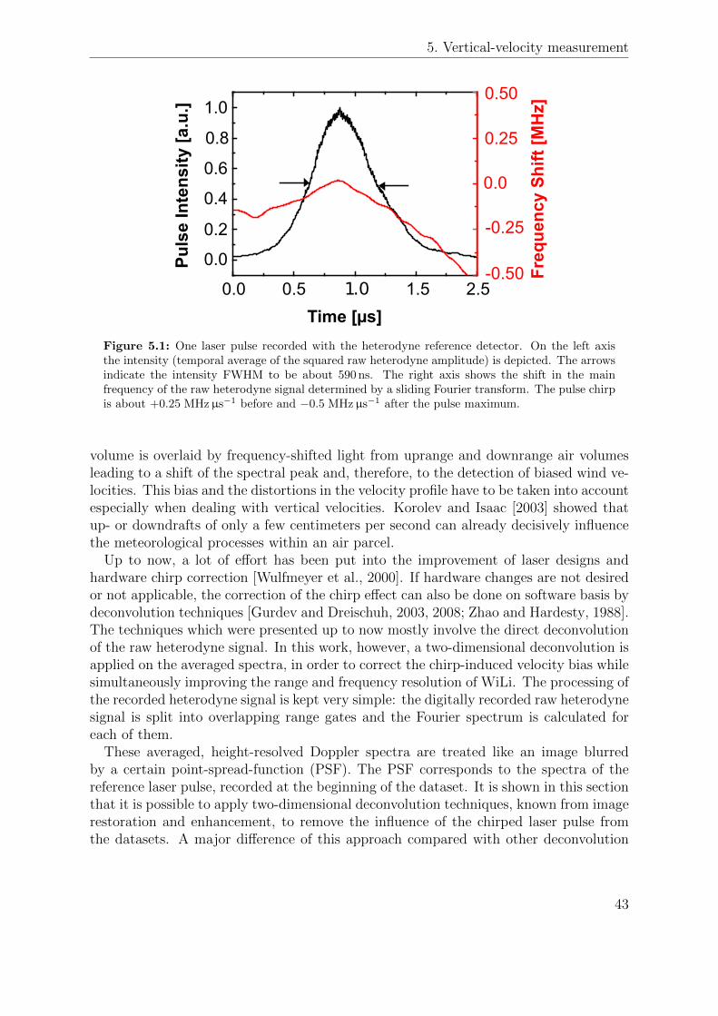
5. Vertical-velocity measurement
-0.50
Time [µs]
Pu
lse
Inte
nsi
ty [
a.u
.]
Fre
qu
ency
Sh
ift
[MH
z]
1.0 1.50.0 0.5 2.5
0.8
1.0
0.6
0.4
0.2
0.0
0.25
0.50
0.0
-0.25
Figure 5.1: One laser pulse recorded with the heterodyne reference detector. On the left axisthe intensity (temporal average of the squared raw heterodyne amplitude) is depicted. The arrowsindicate the intensity FWHM to be about 590 ns. The right axis shows the shift in the mainfrequency of the raw heterodyne signal determined by a sliding Fourier transform. The pulse chirpis about +0.25 MHzµs−1 before and −0.5 MHzµs−1 after the pulse maximum.
volume is overlaid by frequency-shifted light from uprange and downrange air volumesleading to a shift of the spectral peak and, therefore, to the detection of biased wind ve-locities. This bias and the distortions in the velocity profile have to be taken into accountespecially when dealing with vertical velocities. Korolev and Isaac [2003] showed thatup- or downdrafts of only a few centimeters per second can already decisively influencethe meteorological processes within an air parcel.
Up to now, a lot of effort has been put into the improvement of laser designs andhardware chirp correction [Wulfmeyer et al., 2000]. If hardware changes are not desiredor not applicable, the correction of the chirp effect can also be done on software basis bydeconvolution techniques [Gurdev and Dreischuh, 2003, 2008; Zhao and Hardesty, 1988].The techniques which were presented up to now mostly involve the direct deconvolutionof the raw heterodyne signal. In this work, however, a two-dimensional deconvolution isapplied on the averaged spectra, in order to correct the chirp-induced velocity bias whilesimultaneously improving the range and frequency resolution of WiLi. The processing ofthe recorded heterodyne signal is kept very simple: the digitally recorded raw heterodynesignal is split into overlapping range gates and the Fourier spectrum is calculated foreach of them.
These averaged, height-resolved Doppler spectra are treated like an image blurredby a certain point-spread-function (PSF). The PSF corresponds to the spectra of thereference laser pulse, recorded at the beginning of the dataset. It is shown in this sectionthat it is possible to apply two-dimensional deconvolution techniques, known from imagerestoration and enhancement, to remove the influence of the chirped laser pulse fromthe datasets. A major difference of this approach compared with other deconvolution
43

detected Doppler shift
Laserpointing
height
Figure 5.2: Sketch of the chirp effect in vertical-wind velocity observation at cloud bases: Anoptically thick cloud effectively returns a copy of the laser pulse which is recorded by the dataacquisition software. The Fourier analysis yields a lower Doppler shift at the beginning and atthe end of the laser pulse which could be mistaken as negative vertical velocities. The dashedlines represent the height bins of the data acquisition. For simplicity it is shown here without anyinterpolation.
detected Doppler shift
height
aerosolparticles
Figure 5.3: Sketch of the chirp effect in vertical-wind velocity observation within the boundarylayer: An ensemble of particles returns overlapping copies of the laser pulse. Hence, the strongsignal of the center frequency overlaps with chirped lower-frequency signals which effectively shiftsthe frequency peak of the spectra towards lower frequencies. For WiLi, a shift in the detectedvertical velocity of the order of −0.25 m s−1 is introduced. In the case of a Gaussian pulse withonly a chirped tail the effect is the same, for a completely symmetrical chirp however the effectcancels out. The dashed lines represent the height bins of the data acquisition.
44

5. Vertical-velocity measurement
techniques is that it does not need to be employed in real time during data acquisitionand does not need access to the raw heterodyne data. It can be applied to the averagedDoppler spectra, which significantly reduces both the complexity of the data acquisitionsoftware and the amount of data to be stored. In Section 5.1.2, the CDL system WiLiis presented and the laser pulse characteristics are discussed. Subsequently, the two-dimensional deconvolution is introduced (Section 5.1.3.1) and applied to atmosphericdata (Section 5.1.3.2). To further estimate the performance of the two-dimensionaldeconvolution technique, it is applied to a simulated dataset in Section 5.1.4.
5.1.2 Coherent Doppler lidar WiLiThe CDL WiLi of TROPOS is described in detail in Engelmann et al. [2008], so thatonly a brief overview is given here. The lidar is equipped with a master-oscillator-power-amplifier (MOPA) design, operating at a wavelength of 2022 nm. The bandwidth of themaster oscillator (MO) is 150 kHz. The pulse energy of the power oscillator (PO) is 2 mJat a pulse repetition frequency of 750 Hz. In Fig. 5.1, the signal intensity of a recordedlaser pulse is depicted. The change in frequency was determined with a sliding-windowFourier transform and is overlaid in the figure. The trend to negative frequency shiftsat the beginning and at the end of the laser pulse is visible. The pulse chirp is about+0.25 MHzµs−1 before and −0.5 MHzµs−1 after the pulse maximum.
The laser pulse shown in Fig. 5.1 has a length (intensity at full width at half maximum(FWHM), see description of Fig. 5.1) of 590 ns and a spectral width of 720±20 kHz whichis determined from its Fourier spectrum. The spectral width is slightly smaller than thetheoretical bandwidth of 750 kHz (see Eq. (5.2)). This deviation can be explained, ifone considers that the pulse may not be completely Gaussian. It may rather have aslightly asymmetric shape, typical for Q-switched lasers. Yet, for the deconvolutionmethod presented here, the exact pulse length and spectral shape is not important,because the averaged pulse spectrum itself is the reference for the determination of thewind velocities. The measured bandwidth of the laser pulse corresponds to a velocityuncertainty of about ±0.73 m s−1 for one laser shot (Eq. (5.1)). However, after averagingover 1000 laser shots the standard deviation of the reference peak’s frequency fluctuationhas reduced to less than 0.73/
√1000 ≈ 0.02 [m s−1]. Thus, the measurement uncertainty
for the atmospheric wind velocity is no longer determined by the bandwidth of theoutgoing laser pulses, but by the pointing stability of the scanning unit which is about5 mrad for WiLi. For the error estimation, a maximum horizontal wind speed of 20 m s−1
is assumed, which leads to the maximum velocity uncertainty of about 0.10 m s−1 forvertical-wind measurements.
While the laser pulse is emitted by the power amplifier, a small fraction is coher-ently mixed with the light of the master laser at a reference detector. The intermedi-ate frequency of a laser pulse (i.e., the frequency offset between the MO and the PO)is −80 MHz and introduced by an acousto-optical modulator (AOM). The generatedheterodyne signal is recorded with 250 MHz. The light scattered backward from atmo-spheric particles is consecutively detected on another heterodyne detector. For signalswitching, a low-noise high-frequency integrated circuit is used. The two receivers use
45

photodiodes of the same type, have similar amplifiers and their signals are recorded con-secutively by the same data acquisition system. The equal detection and data processingof the laser pulse and the atmospheric signal is very important for the deconvolutionmethod explained here.
The heterodyne signal is recorded for 100 µs after the release of the laser pulse, whichcorresponds to a distance of 15 km in the atmosphere. For one laser shot, the dataacquisition system records 25000 data points which are cut into 200 range gates of 250data points (1 µs), each with an overlap of 125 data points. A Hanning window is appliedin order to suppress sidelobes from discontinuities in the signal. In this way, one rangegate is of 150 m length at interpolated height steps of ∆r = 75 m. On each range gate aFast Fourier Transform (FFT) is performed by extending the dataset to 256 points withzeros. Therefore, the width of one frequency bin is ∆f = 250 MHz
256= 0.977 MHz. With
Eq. (5.1) this corresponds to ∆v = 0.987 m s−1 for one velocity interval. The processingis done in exactly the same way for both the atmospheric signal and the recorded laserpulse, i.e. the laser pulse is also sampled in a range gate with a length of 1 µs. InFig. 5.1 it is visible that even a range gate size of two times the FWHM of the pulsedoes not include the whole pulse. The chirped tail of the pulse is recognized in the nexttwo range gates, too (see also magnification of laser pulse in Fig. 5.4a).
The power spectra are calculated for each range gate of every emitted laser pulse andsummed for an integration time of 1 to 5 s, before they are stored on harddisk. Thisapproach greatly reduces the amount of data from 80 Mbyte s−1 to about 100 kbyte s−1
but, of course, prohibits any re-analysis of the raw heterodyne signal. The further anal-ysis is done by independent software, which searches for the peaks within the averaged
10-10 200-2010-10 200-20
0
1
2
3
4
5
6
a) b)
0
1
2
3
4
5
6
laser pulse
mid-levelcloud(with virga)
boun
dary
laye
r
Hei
gh
t [k
m]
Frequency Shift [MHz]
Figure 5.4: An example of Doppler lidar spectra is shown before (a) and after (b) deconvolution.The data was averaged over 1500 laser shots. Atmospheric features and the laser pulse are labeled.The atmospheric measurement from which this profile is taken is shown in Fig. 5.7 at 17:40 UTC.
46

5. Vertical-velocity measurement
spectra and computes their first moments for velocity estimation. Consecutively, themean velocity in each range gate is calculated with Eq. (5.1).
If the range gates are long enough to include a whole laser pulse (including the chirpedtail, not only the FWHM), the chirp effect does not play a major role. But when theheterodyne signal is interpolated with range gates smaller than the laser pulse itself,chirp-induced artifacts as described in Section 5.1.1 will appear. Indeed, the bias forcontinuous signals could be avoided by using the average frequency of the whole outgoinglaser pulse as reference frequency. This averaging would largely compensate for the bias,but would in turn shift the velocities at cloud bases into the opposite direction towardspositive velocities. Also, the range resolution would be decreased. Therefore, the onlypossibility to have at the same time correct values at cloud bases and within the boundarylayer is to resolve the frequency chirp of the laser pulse in different range gates and usethis information to remove the chirp artifacts. In the following section, a deconvolutiontechnique is presented that is capable of removing the chirp artifacts from cloud basesand continuous signals at once.
5.1.3 Application of two-dimensional deconvolution toatmospheric Doppler spectra
5.1.3.1 Method
Let D∗(ρ = 0 . . . Nρ, ν = 0 . . . Nν) contain the pure and undisturbed information aboutthe intensity scattered back from each element of the discrete range–frequency space.The discrete coordinates are connected with the continuous coordinates like r = ρ∆rand f = ν∆f .
The formation of the atmospheric power spectra Pc(ρ, ν) (see Eq. (3.7)) in the receivercan be described by a convolution of D∗(ρ, ν) with a suitable PSF PPSF(ρ, ν). In thiscontext, the PSF consists of the averaged power spectra of the chirped laser pulse at thebeginning of the datasets (from ρ = 0 . . . 4):
Pc(ρ, ν) =
Ni∑i=−Ni
Nj∑j=−Nj
D∗(ρ− i, ν − j)PPSF(i, j). (5.3)
(2Ni + 1) and (2Nj + 1) are the frequency and the range extent of the PSF, respectively.Application of the convolution theorem [Goodman, 2005a] on Eq. (5.3) yields
DFT[Pc(ρ, ν)] = DFT[D∗(ρ, ν)]DFT[PPSF(ρ, ν)], (5.4)
with the Discrete Fourier Transformation DFT. For this case, of course, PPSF(ρ, ν) hasto be extended with zero values to be of the same size as D∗(ρ, ν).
Removing the effect of the chirped laser pulse from the dataset requires to undo theconvolution operation in order to recover the original atmospheric information D∗(ρ, ν).Theoretically, it is possible to divide Eq. (5.4) by DFT[PPSF(ρ, ν)] and to apply an in-verse Fourier transformation afterwards. However, this approach usually fails, because
47

a)
b) c)
Figure 5.5: Example of two-dimensional deconvolution. The image of the Hotel-Dieu de Lyonin (a) is blurred, because the camera was moved during exposure. From the street lights that arepictured in front of a darker background, it is visible that the camera was moved in a half-circle.The undisturbed image of such a street light can be assumed point-like, so that its blurred imagecan be used as a PSF for deconvolution (b). The resulting deconvolved image is shown in (c). Theimage was taken at Lyon, France on 8 December 2007.
48

5. Vertical-velocity measurement
of noise amplification. The direct inversion of the deconvolution by solving the equa-tion system presented by Eq. (5.3) is also not possible, because the equation system isunderdetermined. Therefore, an iterative deconvolution algorithm has to be applied inorder to retrieve an approximation of the input information D∗(ρ, ν).
Iterative two-dimensional deconvolution algorithms are best known from confocal mi-croscopy [Baddeley et al., 2006] and astronomy. For the application presented here, theRichardson–Lucy (RL) algorithm is used [Richardson, 1972; Lucy, 1974]. It is famousfor its application on blurred images of the Hubble Space Telescope [Stobie et al., 1994].But this algorithm is not the only one available. There exist various other algorithmswhich could be applied here, too. Most of them are already available in ready-to-usesoftware packages. An example of a deconvolution applied on a blurred photographicpicture is shown in Fig. 5.5. A flowchart of the deconvolution operation is given inFig. 5.6.
The RL algorithm is an iterative algorithm, which tries to reproduce the functionPc(ρ, ν) (Eq. (5.3)) by making an initial guess of D∗(ρ, ν) and then convolving this guesswith a provided point spread function PPSF(ρ, ν). The initial guess can, e.g., be providedby directly solving Eq. (5.4) as explained above, or it can be the disturbed dataset itself.The disparity between the resulting dataset P ∗c (ρ, ν) and Pc(ρ, ν) is then used to makea better estimate of D∗(ρ, ν) in the next iteration step. The iteration is stopped aftera defined number of steps, or when the difference between P ∗c (r, f) and Pc(r, f) hasbecome smaller than a defined threshold. In order to increase the convergence speed ofthe RL algorithm, a vector-extrapolation-based acceleration technique is used here [Biggsand Andrews, 1997; Remmele and Hesser, 2009]. P ∗c (r, f) can serve as a test function
Main Loop
Blurredinput data
P
Guess undisturbed dataset
D*
Convolve D* with PSF to obtain
P*
Compare P and P* to improve guess
Output D*
Figure 5.6: Illustration of the forward-iteration procedure for two-dimensional deconvolution.The main step is the guessing of the unknown function D∗ and the consecutive convolution withthe known PSF. The deviations between P and P ∗ are then used to make a better guess in thenext step.
49

to determine whether the deconvolution was successful or not. If P ∗c (r, f) convergestowards a shape strongly different from Pc(r, f), it may, e.g., indicate that an incorrectPSF was used. This test will be applied later in this work during the deconvolution ofradar spectra in Chapter 7.
A lot of different software solutions exist which can perform an iterative two-dimensio-nal deconvolution. For this work, the implementation of the RL algorithm of the imagerestoration software “BiaQIm” [Tadrous, 2011] was used. It was favorable, because it hascommand-line access and can read arbitrary floating-point data. On a desktop computerthe software needs less than one second for the deconvolution of one dataset with 196range gates. Since the acquisition time for one dataset is at minimum 1 s, for WiLi theoperation can be performed in real time during measurements, but it can also be appliedafterwards on the stored spectra. Both types of operation have been implemented in thecontext of this work.
5.1.3.2 Improvement of the velocity estimation for atmospheric data
Figure 5.7 shows an example of an atmospheric measurement with the vertically pointingWiLi at Leipzig on 13 March 2011. The top two panels show the signal intensity (in thefollowing, the term “intensity” is used to describe the estimated amplitude of a signalpeak after background subtraction), the vertical velocity within the planetary boundarylayer (0 to 3 km height) and the terminal velocity of ice particles and water droplets inthe virgae of altocumulus clouds (3 to 6 km height). The spectra were averaged over1500 laser shots (2 s). The chirp effect is visible above and below clouds (e.g., in themagnified portion) and at positions where the intensity is very high. At the bottomand at the top of those structures negative velocities seem to appear, which could bemistaken as falling particles or downdrafts. These artifacts originate from backscatteredlight from the beginning (bottom chirp effect) and from the end (top chirp effect) of thelaser pulse.
To correct the chirp effect in the entire measurement of Fig. 5.7, the RL algorithmwas applied on each 2-s dataset independently with ten iteration steps. The result isshown in Fig. 5.7c and 5.7d. The velocities within the optically thin cloud layers and theboundary layer are shifted and there is no longer an overall trend to negative vertical-velocity values. The removal of the velocity bias is nicely visible in the boundary layerfrom 17:30 to 18:00 UTC. The deconvolution shifts the detected wind velocities by about0.25 m s−1 towards positive values. Artificial velocities at the cloud bases and the cloudtops are no longer present. The method works equally for weak and strong signals.
Figure 5.4a presents an example profile, marked with a dotted line at 17:40 UTC in theatmospheric measurement of Fig. 5.7. The chirped laser pulse is magnified. The datasetwas deconvolved with the accelerated RL algorithm (10 iterations) using the recordedlaser pulse at the beginning of the dataset as a PSF. Fig. 5.8 shows a comparison betweenthe vertical velocities estimated from the untreated (Fig. 5.8a) and the deconvolveddataset (Fig. 5.8b). In Fig. 5.4b it is visible that the recorded reference laser pulse hasbeen reduced to nearly one bin in range and frequency dimension. That means that nowthe resolution of the dataset matches the grid and is close to its theoretical maximum.
50

5. Vertical-velocity measurement
1
2
3
4
5
6
-2
-1
0
1
2
1
2
3
4
5
6
-2
0
2
4
6
8
17:00 17:10 17:20 17:30 17:40 17:50
1
2
3
4
5
6
-2
-1
0
1
2
1
2
3
4
5
6
-2
0
2
4
6
8
18:00
a)
b)
c)
d)In
ten
sity
(lo
g)
[a.u
.]V
erti
cal V
elo
city
[m
s⁻¹
]
Inte
nsi
ty (
log
) [
a.u
.]V
erti
cal V
elo
city
[m
s⁻¹
]
Hei
gh
t [k
m]
Hei
gh
t [k
m]
Hei
gh
t [k
m]
Hei
gh
t [k
m]
Time [UTC]Figure 5.7: Application of the deconvolution technique on a measurement of WiLi performed atLeipzig on 11 March 2011. In a) and b) the signal intensities and the vertical velocity distribution ofan atmospheric measurement of the boundary layer and mid-level cloud layers are depicted. In thered box the chirp effect is visible above and below the cloud as artificial negative velocities (greencolor). c) and d) show the same measurement after correction of the chirp effect by deconvolution.The dashed red line at 17:40 UTC indicates the position of the example measurement shown inFig. 5.4. The chirp effect is visible above and below the cloud layers in the magnified portions ofthe velocity plots.
51

0
1
2
3
4
5
6
10-7 10-5 10-3 10-1 -1 0 1
noise level
Hei
gh
t [k
m]
Normalized Intensity
Vertical Velocity[m s⁻¹]
Figure 5.8: Signal intensities (left) and velocities (right) calculated by means of the peak-findingsoftware from the raw atmospheric dataset (black line) and from the deconvolved dataset (redline). The input data is depicted in Fig. 5.4a and b.
5.1.3.3 Improvement of the range resolution
The deconvolution technique presented in this work does not only correct the chirpeffect. It also simultaneously improves the range and the frequency resolution of thespectra. The improvement of the range resolution is visible, e.g., in Fig. 5.4 between 3and 6 km height. The single layers are much better separated after the deconvolutionmethod has been applied. In Fig. 5.7c the features within the cloud layers are also muchmore distinct than in Fig. 5.7a. The qualification of the resolution improvement is givenin Section 5.1.4.
5.1.3.4 Improvement of the frequency resolution
In most cases, a frequency resolution improvement is not needed because only one spec-tral peak is present (e.g., Fig. 5.7). But there are certain conditions under which animprovement of the frequency resolution can be of advantage. Fig. 5.9a shows spectraaveraged over 5 s (3600 laser shots) that were observed on 29 March 2006, when the onsetof rainfall was recorded in low-level clouds at 750 m height. At that height, the spectrasplit and two peaks appear. Here, water drops (likely drizzle) fall with −3.5 m s−1 outof the cloud, which itself is composed of smaller droplets which move slowly upwards at0.2 m s−1. Fig. 5.10 shows the Doppler frequency shift between the arrows in Fig. 5.9aand 5.9b. After deconvolution the peaks are much better separated. This case alsohighlights that it is possible to apply the deconvolution procedure on historic datasets.
52

5. Vertical-velocity measurement
20100-10-20
0
1
2
3
20100-10-20
0
1
2
3
a) b)
Hei
gh
t [k
m]
Frequency Shift [MHz]
Figure 5.9: Comparison between (a) the raw atmospheric and (b) the deconvolved Doppler spectrarecorded during rainfall at Leipzig on 29 March 2006. Double peaks resulting from upwards drivenaerosol particles and falling raindrops, respectively, are visible in the spectra at about 750 m height.The two spectra marked by arrows are shown in Fig. 5.10. (The structure at 1.5 km height and15 MHz is an artifact, presumably resulting from a weak parasiteric laser line of the MO. Yet, thisdoes not affect the central part of the spectrum.)
-6 -4 -2 0 2 4 60.0
0.2
0.4
0.6
0.8
1.0
1.2
Frequency Shift [MHz]
No
rmal
ized
Inte
nsi
ty
Deconvolved (10 iter.)Original
aerosolparticles
fallingdroplets
Figure 5.10: Atmospheric Doppler spectra during the rainfall event of Fig. 5.9. The improvementof frequency resolution between the original dataset (black line) and the deconvolved dataset (redline) is visible.
53
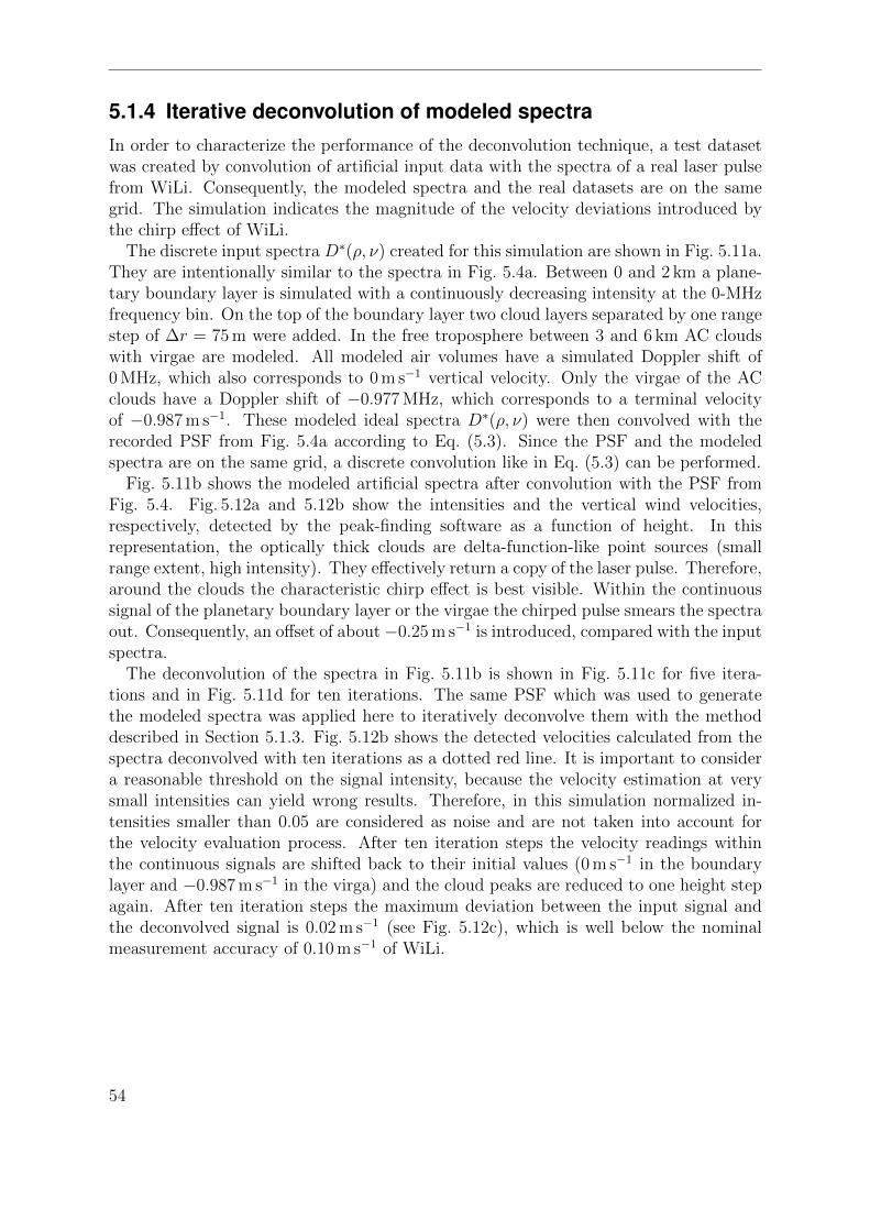
5.1.4 Iterative deconvolution of modeled spectraIn order to characterize the performance of the deconvolution technique, a test datasetwas created by convolution of artificial input data with the spectra of a real laser pulsefrom WiLi. Consequently, the modeled spectra and the real datasets are on the samegrid. The simulation indicates the magnitude of the velocity deviations introduced bythe chirp effect of WiLi.
The discrete input spectra D∗(ρ, ν) created for this simulation are shown in Fig. 5.11a.They are intentionally similar to the spectra in Fig. 5.4a. Between 0 and 2 km a plane-tary boundary layer is simulated with a continuously decreasing intensity at the 0-MHzfrequency bin. On the top of the boundary layer two cloud layers separated by one rangestep of ∆r = 75 m were added. In the free troposphere between 3 and 6 km AC cloudswith virgae are modeled. All modeled air volumes have a simulated Doppler shift of0 MHz, which also corresponds to 0 m s−1 vertical velocity. Only the virgae of the ACclouds have a Doppler shift of −0.977 MHz, which corresponds to a terminal velocityof −0.987 m s−1. These modeled ideal spectra D∗(ρ, ν) were then convolved with therecorded PSF from Fig. 5.4a according to Eq. (5.3). Since the PSF and the modeledspectra are on the same grid, a discrete convolution like in Eq. (5.3) can be performed.
Fig. 5.11b shows the modeled artificial spectra after convolution with the PSF fromFig. 5.4. Fig. 5.12a and 5.12b show the intensities and the vertical wind velocities,respectively, detected by the peak-finding software as a function of height. In thisrepresentation, the optically thick clouds are delta-function-like point sources (smallrange extent, high intensity). They effectively return a copy of the laser pulse. Therefore,around the clouds the characteristic chirp effect is best visible. Within the continuoussignal of the planetary boundary layer or the virgae the chirped pulse smears the spectraout. Consequently, an offset of about−0.25 m s−1 is introduced, compared with the inputspectra.
The deconvolution of the spectra in Fig. 5.11b is shown in Fig. 5.11c for five itera-tions and in Fig. 5.11d for ten iterations. The same PSF which was used to generatethe modeled spectra was applied here to iteratively deconvolve them with the methoddescribed in Section 5.1.3. Fig. 5.12b shows the detected velocities calculated from thespectra deconvolved with ten iterations as a dotted red line. It is important to considera reasonable threshold on the signal intensity, because the velocity estimation at verysmall intensities can yield wrong results. Therefore, in this simulation normalized in-tensities smaller than 0.05 are considered as noise and are not taken into account forthe velocity evaluation process. After ten iteration steps the velocity readings withinthe continuous signals are shifted back to their initial values (0 m s−1 in the boundarylayer and −0.987 m s−1 in the virga) and the cloud peaks are reduced to one height stepagain. After ten iteration steps the maximum deviation between the input signal andthe deconvolved signal is 0.02 m s−1 (see Fig. 5.12c), which is well below the nominalmeasurement accuracy of 0.10 m s−1 of WiLi.
54

5. Vertical-velocity measurement
Frequency Shift [MHz]
-10 0 10 -10 0 10 -10 0 10 -10 0 10
Hei
gh
t [k
m]
Figure 5.11: Overview of the different steps of the simulation: a) ideal input spectra, b) rawspectra as they would be detected by the wind lidar, spectra deconvolved with 5 iterations (c) and(d) with 10 iterations.
a) b) c)
0
1
2
3
4
5
0.0 0.5 1.0 -1.5 -1.0 -0.5 0.0 -0.02 0.00 0.02
input data (idealized)convolved with chirped laser pulsedeconvolved output
Normalized Intensity Vertical Velocity [m s⁻¹]Residual
Velocity Error [m s⁻¹]
Hei
gh
t [k
m]
Figure 5.12: Intensities (a) and vertical wind velocities (b) calculated with the evaluation soft-ware from the simulated datasets (Fig. 5.11a, b and d). Thick gray lines: idealized input data(Fig. 5.11a), solid green lines: results from the simulated raw spectra (Fig. 5.11b), dotted redlines: results after deconvolution of the simulated spectra with 10 iterations (Fig. 5.11d). Panel(c) shows the difference in the velocity estimation between the idealized input data and the decon-volved spectra. It is visible that the deconvolution removes the chirp effect and that the deviationbetween the ideal input data and the deconvolved data is less than 0.02 m s−1.
55

5.1.5 Usage of deconvolution in the scope of this workThe presented deconvolution method enables WiLi to reach a very high velocity accuracyin the range of 0.05 to 0.10 m s−1. The final accuracy is no longer determined by thechirp effect, but by other factors, e.g., the pointing stability of the scanning unit. Thedeconvolution technique can be applied on stored averaged spectra or in real time duringthe measurement. Both variants have been implemented in the context of this work.Historical datasets, like that of the SAMUM-2 campaign, were also deconvolved, becauseaveraged spectra had been stored during the operation of WiLi. The method works, evenif the shape of the chirp changes over time, and can also be applied in chirp-free casesto simply increase the range and frequency resolution. The RL algorithm has beendesigned for general purposes and can be used for deconvolution of any dataset, if onlya suitable PSF is available. It is worth noting that the algorithm does not requireany assumptions about the undisturbed dataset, but only takes available informationabout the measurement process to remove disturbances. Therefore, the experience withdeconvolution operations, gained in the development of the chirp correction, is furtherused in this work. In Chapter 7, a one-dimensional version of the RL algorithm is appliedfor the correction of spectral broadening in cloud-radar spectra.
5.2 Cloud-radar data processingThe MIRA-35 cloud radar (see Fig. 5.13) emits electromagnetic pulses with a pulserepetition frequency of 5000 Hz, a wavelength of 8 mm and a pulse length of 300 ns. Itrecords a heterodyne signal by mixing the backscattered radiation with a narrow-bandreference wave. Two orthogonally polarized channels are recorded simultaneously. Inboth channels, the signal processor directly measures and stores the complex amplitudeof the incoming radiation for each shot in each range gate. After 256 shots, a Fouriertransformation is applied on all stored complex amplitudes of each range gate. In thisway, two Fourier spectra are obtained: one co- and one cross-polarized spectrum. Fourierspectra are averaged for 10 s and stored temporarily on harddisk. In this configuration,the velocity resolution is about 0.08 m s−1 and the range resolution is about 30 m. Thecomplete signal recording and processing of the MIRA-35 cloud radar system is describedby Bauer-Pfundstein and Gorsdorf [2007].
From the raw spectra all other cloud radar products are derived:
• Radar reflectivity factor Z: The values in co- and cross channels are quadraticallysummed up to a total power spectrum. Z is the integral of this spectrum, afternoise subtraction, range correction and multiplication with the system constant ofthe radar.
• Mean velocity v: first moment of the total power spectrum.
• Linear depolarization ratio δ (LDR): ratio of the summed power in the cross- andco-spectra.
56
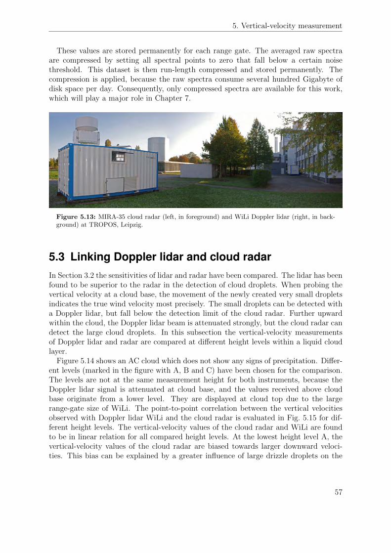
5. Vertical-velocity measurement
These values are stored permanently for each range gate. The averaged raw spectraare compressed by setting all spectral points to zero that fall below a certain noisethreshold. This dataset is then run-length compressed and stored permanently. Thecompression is applied, because the raw spectra consume several hundred Gigabyte ofdisk space per day. Consequently, only compressed spectra are available for this work,which will play a major role in Chapter 7.
Figure 5.13: MIRA-35 cloud radar (left, in foreground) and WiLi Doppler lidar (right, in back-ground) at TROPOS, Leipzig.
5.3 Linking Doppler lidar and cloud radarIn Section 3.2 the sensitivities of lidar and radar have been compared. The lidar has beenfound to be superior to the radar in the detection of cloud droplets. When probing thevertical velocity at a cloud base, the movement of the newly created very small dropletsindicates the true wind velocity most precisely. The small droplets can be detected witha Doppler lidar, but fall below the detection limit of the cloud radar. Further upwardwithin the cloud, the Doppler lidar beam is attenuated strongly, but the cloud radar candetect the large cloud droplets. In this subsection the vertical-velocity measurementsof Doppler lidar and radar are compared at different height levels within a liquid cloudlayer.
Figure 5.14 shows an AC cloud which does not show any signs of precipitation. Differ-ent levels (marked in the figure with A, B and C) have been chosen for the comparison.The levels are not at the same measurement height for both instruments, because theDoppler lidar signal is attenuated at cloud base, and the values received above cloudbase originate from a lower level. They are displayed at cloud top due to the largerange-gate size of WiLi. The point-to-point correlation between the vertical velocitiesobserved with Doppler lidar WiLi and the cloud radar is evaluated in Fig. 5.15 for dif-ferent height levels. The vertical-velocity values of the cloud radar and WiLi are foundto be in linear relation for all compared height levels. At the lowest height level A, thevertical-velocity values of the cloud radar are biased towards larger downward veloci-ties. This bias can be explained by a greater influence of large drizzle droplets on the
57

a) WiLi intensity109
105
Sig
nal I
nten
sity
[a.u
.]
Hei
ght [
m]
100
b) WiLi vertical velocity
Ver
tical
Vel
ocity
[m s⁻¹
]
Hei
ght [
m]
AB
C
c) MIRA-35 radar signal-to-noise ratio
SN
R [d
B]
Hei
ght [
m]
d) MIRA-35 vertical velocity
Ver
tical
Vel
ocity
[m s⁻¹
]
Hei
ght [
m]
ABC
Figure 5.14: Intensity (a) and vertical velocity (b) of Doppler lidar WiLi together with MIRA-35radar reflectivity (c) and vertical velocity (d) for a short section of an AC cloud recorded at Leipzigon 1 August 2012.
cloud-radar signal at this height level. The slope of the correlation line between thecloud radar and WiLi data is smaller than one at all compared height levels, meaningthat the cloud radar shows smaller vertical velocities than WiLi. This difference canoccur, e.g, from slightly mismatched height levels, if spherical turbulent structures areassumed. The correlation between the vertical velocities also confirms that the valuesdetected by WiLi above 3300 m height actually originate from a lower level. Some valuesare detected by the Doppler lidar at the highest level C, because one range gate extends50% into the neighboring ones and there is no other signal received within the highestrange gate. However, the proportionality to the respective values of the cloud radarindicates that the vertical-velocity values of WiLi are independent and actually deliverheight-resolved information.
For the same cloud section, the averaged profiles of vertical velocity and signal strengthof both WiLi and cloud radar are shown in Fig. 5.16. The gray lines indicate theaverage of all profiles, while the orange and green lines represent profiles of updraftsand downdrafts, respectively. An average vertical velocity of ±0.1 m s−1 was used as athreshold to sort the profiles into updrafts and downdrafts, respectively. In Fig. 5.16a theaveraged signal strengths of both systems is shown, while Fig. 5.16b depicts the averageprofiles of vertical velocity. WiLi already detects vertical velocities at about 3150 mheight, while the radar shows its first measurement value 80 m higher at 3230 m. Abovethat level, the averaged vertical-velocity profiles of WiLi and the cloud radar agree withinabout ±0.1 m s−1, i.e, within the measurement accuracy of both systems. In this case,the pointing error is critical, because a tilt would introduce a component of the advectionvelocity into the measured vertical velocity. A deviation of no more than 0.1 off-zenithis desired. This pointing accuracy is difficult to accomplish, especially for the cloud
58

5. Vertical-velocity measurement
a)
Rad
ar [m
s⁻¹
]
−1
0
1
Lidar [m s⁻¹]−1 0 1
m = 0.9±0.05c = -0.2±0.02 m s⁻¹R² = 0.74
b)
Rad
ar [m
s⁻¹
]
−1
0
1
Lidar [m s⁻¹]−1 0 1
m = 0.79±0.03c = -0.03±0.01 m s⁻¹R² = 0.77
c)
Rad
ar [m
s⁻¹
]
−1
0
1
Lidar [m s⁻¹]−1 0 1
m = 0.77±0.03c = 0.04±0.01 m s⁻¹R² = 0.65
Figure 5.15: Correlation plots for horizontal levels marked in Fig. 5.14. Levels A, B and Ccorrespond to plots (a), (b) and (c), respectively. For the whole one-hour time period, pairs ofvalues from WiLi and cloud radar are plotted. The time resolution of WiLi was reduced to 10 s byaveraging of 5 adjacent values to match the time resolution of the cloud radar. A linear functionf(x) = mx+ c is fitted to each dataset. In panel (a) only sporadic measurements are found in thecloud radar dataset. The existing velocity pairs show the best linearity (m ≈ 0.9), but they arebiased (c ≈ −0.2 m s−1). At height levels B and C the slope is smaller (m ≈ 0.8) but the bias isvery low (within ±0.05 m s−1).
a)
Lida
r Int
ensi
ty [a
.u]
1.4×10⁹
1.6×10⁹
1.8×10⁹
2.0×10⁹
2.2×10⁹
2.4×10⁹
2.6×10⁹
Clo
ud R
adar
Z [d
BZ]
−30
−25
−20
−15
−10
−5
Height [m]3150 3200 3250 3300 3350 3400
Lidar Radar All Updrafts Downdrafts
b)
Aver
age
Vert
ical
Vel
ocity
[m s⁻¹
]
−0.6
−0.4
−0.2
0
0.2
0.4
0.6
0.8
Height [m]3150 3200 3250 3300 3350 3400
Lidar Radar All Updrafts Downdrafts
Figure 5.16: Mean Doppler lidar and cloud radar signal (a) and vertical velocity (b) of the cloudsection depicted in Fig. 5.14. The averaged values are only shown, if more than 10 values werepresent in the whole time and height section.
radar, which has only limited means of precision leveling. Hence, it is very pleasing tofind both systems in such good agreement. This comparison is essentially enabled bythe deconvolution method described in Section 5.1. With the help of this method itis shown here for the first time that height-resolved vertical-velocity information fromcloud bases can be derived with Doppler lidar, even with a long pulse length of about180 m.
59
5.4 Capabilities of lidar and radar to probe turbulenceThe structure of layered clouds is the result of turbulent motion inside the cloud layer.Sources of turbulent motion can be, e.g., wind shear, radiative cooling at cloud topor gravity waves. Energy introduced into the system leads to the development of largeeddies, which consecutively break down into many smaller eddies. This process dissipatesthe turbulent energy towards smaller and smaller sizes eventually reaching the molecularlevel, where energy is converted from mechanical energy into heat. Kolmogorov [1941]proposed that the power spectrum of turbulent energy dissipation is given by
E(k) = Cε23k−
53 . (5.5)
E(k) is the energy per unit volume, C ≈ 0.5 the Kolmogorov constant, ε the energydissipation rate and k = 2π
Λthe wavenumber (with Λ the corresponding structure size).
The variance of one velocity component within this turbulent field is
σ2 =
∫ ∞0
E(k) dk, (5.6)
with the standard deviation σ.Usually, layered clouds are embedded into a turbulent layer, topped by an inversion
layer. This inversion restricts the maximum size of the turbulent eddies. Only eddieswith a size Λ smaller than two times the layer depth dl can move freely. The wavenumberat which turbulent motion becomes visible in the energy spectrum is hence kl = π/dl.
In Fig. 5.17 turbulent-energy spectra of the AC cloud from Fig. 5.14 are depicted. Thespectra were calculated from the vertical velocities measured with WiLi and the cloudradar at height level B in Fig. 5.14. The transition from time to spatial frequencieswas made by application of Taylor’s hypothesis [Taylor, 1938], which assumes k = 2π
uaf .
The mean advection speed ua at cloud base has been taken from the GDAS dataset.The bold lines in Fig. 5.17 are smoothed versions of the corresponding energy spectra.The energy spectrum of the cloud radar is smaller than that of WiLi by a constantfactor. This difference can, again, be explained by a non-perfect match in height levels.However, the shapes of the averaged curves are similar, meaning that the cloud radarand WiLi show the same frequency response below an integration time of 10 s.
With the help of this description, the capabilities of Doppler lidar and cloud radarfor measuring turbulent motion within cloud layers can be estimated. For that purpose,a model of a simple energy spectrum is used: For spatial frequencies k < kl let the
energy be constant at E0!
= Cε23k− 5
3l , for k > kl the energy spectrum is assumed to
be proportional to k−53 . Continuity is demanded at kl. These assumptions reproduce
energy spectra similar to those depicted in Fig. 5.17, but without noise, and Eq. (5.6)can be solved analytically:
60

5. Vertical-velocity measurement
Turb
ule
nt
En
erg
y [m
³ s⁻
²]
10−4
10−3
10−2
10−1
100
101
Wave Number [m⁻¹]10−4 10−3 10−2 10−1
Doppler Lidar Doppler Lidar smoothed Cloud Radar Cloud Radar smoothedE(k) = 0.5 (3.5×10⁻⁴)2/3 k-5/3
kc
Radarkc
Lidarkl
Figure 5.17: Comparison between the turbulent energy spectra of Doppler lidar and cloudradar. The advection speed taken from the GDAS dataset is ua = 7.5 m s−1. The character-istic wavenumber is found to be kl = 0.01 m−1. Standard deviations are σL = 0.39 m s−1 for WiLiand σR = 0.28 m s−1 for the cloud radar. The blue curve indicates the energy spectrum for adissipation rate of ε = 3.5× 10⁻⁴ m 2s−3 and C = 0.5.
σ2 = Cε23
(k− 5
3l
∫ kl
0
dk +
∫ kc
kl
k−53 dk
)(5.7)
= Cε23
(5
2k− 2
3l −
3
2k− 2
3c
). (5.8)
kc = πΛc
= π∆tua
is the cut-off wavenumber, which depends on the advection speedand the measurement interval ∆t. For an ideal measurement system ∆t→ 0 and conse-
quently k− 2
3c → 0. In Table 5.1 values for the standard deviation σ and the corresponding
variance σ2 are shown, which have been calculated with Eq. (5.8). The numeric valuesof C×ε and kl have been taken from the real measurement of Fig. 5.17. Whilst the stan-dard deviation gives a direct impression of the order of magnitude of the vertical-velocityvalues, the variance is a measure for the turbulent kinetic energy (TKE). These calcula-tions isolate the effect of time resolution. The values of variance and standard deviationare also proportional to the strength of the recorded vertical-velocity values. Therefore,variance and standard-deviations for the cloud radar are overestimated, because it de-tects slightly lower vertical-velocity values and, hence, a smaller energy-dissipation rate
61
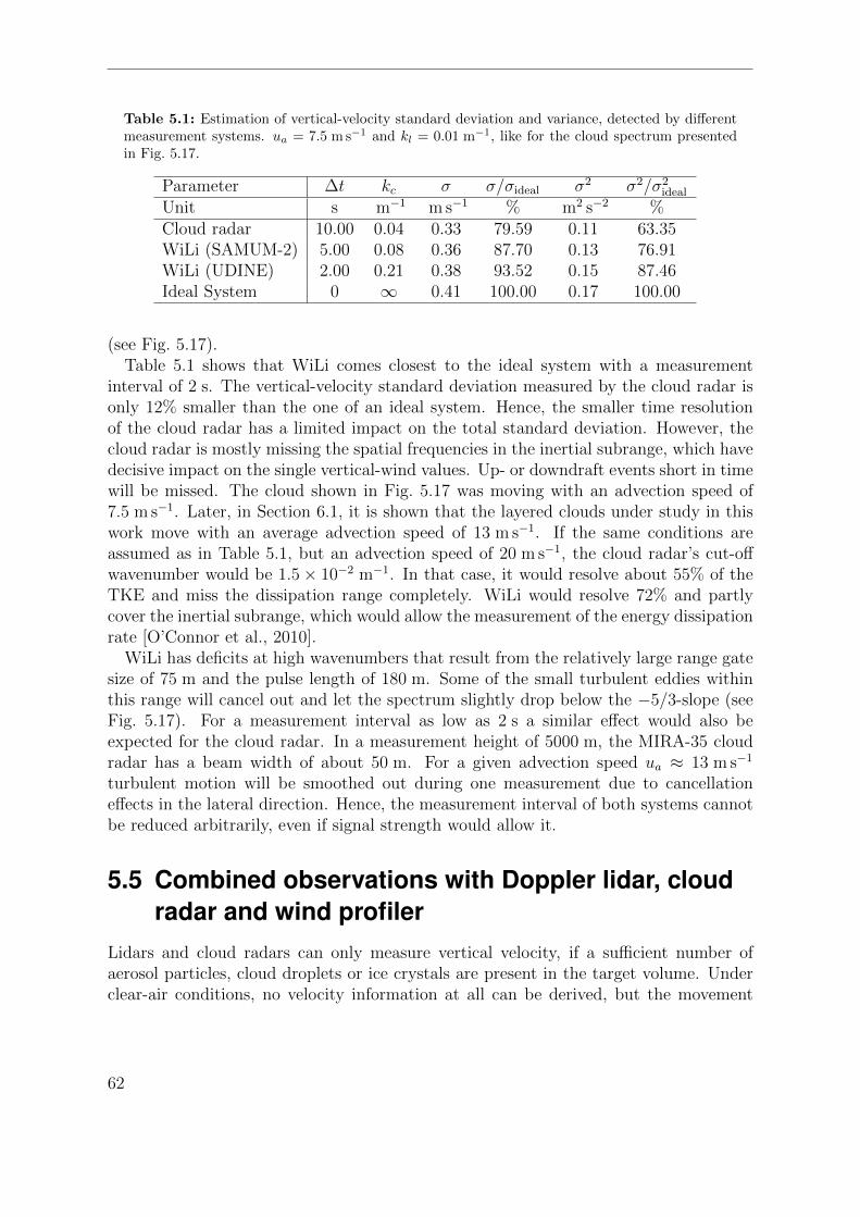
Table 5.1: Estimation of vertical-velocity standard deviation and variance, detected by differentmeasurement systems. ua = 7.5 m s−1 and kl = 0.01 m−1, like for the cloud spectrum presentedin Fig. 5.17.
Parameter ∆t kc σ σ/σideal σ2 σ2/σ2ideal
Unit s m−1 m s−1 % m2 s−2 %Cloud radar 10.00 0.04 0.33 79.59 0.11 63.35WiLi (SAMUM-2) 5.00 0.08 0.36 87.70 0.13 76.91WiLi (UDINE) 2.00 0.21 0.38 93.52 0.15 87.46Ideal System 0 ∞ 0.41 100.00 0.17 100.00
(see Fig. 5.17).Table 5.1 shows that WiLi comes closest to the ideal system with a measurement
interval of 2 s. The vertical-velocity standard deviation measured by the cloud radar isonly 12% smaller than the one of an ideal system. Hence, the smaller time resolutionof the cloud radar has a limited impact on the total standard deviation. However, thecloud radar is mostly missing the spatial frequencies in the inertial subrange, which havedecisive impact on the single vertical-wind values. Up- or downdraft events short in timewill be missed. The cloud shown in Fig. 5.17 was moving with an advection speed of7.5 m s−1. Later, in Section 6.1, it is shown that the layered clouds under study in thiswork move with an average advection speed of 13 m s−1. If the same conditions areassumed as in Table 5.1, but an advection speed of 20 m s−1, the cloud radar’s cut-offwavenumber would be 1.5× 10⁻² m−1. In that case, it would resolve about 55% of theTKE and miss the dissipation range completely. WiLi would resolve 72% and partlycover the inertial subrange, which would allow the measurement of the energy dissipationrate [O’Connor et al., 2010].
WiLi has deficits at high wavenumbers that result from the relatively large range gatesize of 75 m and the pulse length of 180 m. Some of the small turbulent eddies withinthis range will cancel out and let the spectrum slightly drop below the −5/3-slope (seeFig. 5.17). For a measurement interval as low as 2 s a similar effect would also beexpected for the cloud radar. In a measurement height of 5000 m, the MIRA-35 cloudradar has a beam width of about 50 m. For a given advection speed ua ≈ 13 m s−1
turbulent motion will be smoothed out during one measurement due to cancellationeffects in the lateral direction. Hence, the measurement interval of both systems cannotbe reduced arbitrarily, even if signal strength would allow it.
5.5 Combined observations with Doppler lidar, cloudradar and wind profiler
Lidars and cloud radars can only measure vertical velocity, if a sufficient number ofaerosol particles, cloud droplets or ice crystals are present in the target volume. Underclear-air conditions, no velocity information at all can be derived, but the movement
62

5. Vertical-velocity measurement
2 Ceilometers
UHFWind Profiler
MIRA-35Cloud Radar
StreamlineDoppler Lidar
Figure 5.18: Aerial view of the wind profiler site at MOL (Image Credit: DWD). The photographwas taken in September 2011. In the meantime a Streamline Doppler lidar and a MIRA-35 cloudradar were deployed next to the wind profiler (red areas).
of clear air is actually an important measurement quantity. Large-scale atmosphericmotion (e.g., gravity waves) can influence a cloud decisively, and falling droplets or icecrystals are slowed down or accelerated by vertical air movements.
Wind-profiler radars have been designed to measure the movement of the clear air.While the radar technique itself is nearly 70 years old, the wind profiler technique hasbeen developed not before the late 1970s [Strauch et al., 1984; Weber and Wuertz,1990]. A wind profiler exploits Bragg scattering at atmospheric density fluctuations toproduce a backscatter signal even under clear-air conditions. Rayleigh scattering fromparticles also adds to the signal, but as the efficiency of Rayleigh and Bragg scatteringis proportional to λ−4 and λ−
13 , respectively, Bragg scattering dominates more and more
for longer wavelengths.The distribution of powerful wind profilers is limited, but they can actually deliver
the desperately needed information about the velocity of clear air. They can only beoperated by a limited number of well-funded institutions, due to their high operationalcosts. The DWD operates an ultra-high frequency (UHF) wind profiler at MOL (seeFig. 5.18). It works at 482 MHz and can deliver wind information from 0.5 km to 10 kmheight with a range resolution of 150 m, a measurement interval of about 10 s and avelocity resolution of about 0.1 m s−1 [Bohme et al., 2004]. The distance between twoneighboring range gates is 94 m due to range interpolation.
5.5.1 Combined observation strategy and case studiesIn the context of this work, a cooperation between MOL and TROPOS has been es-tablished in July 2013. Combined measurements of the vertical velocity were carriedout simultaneously with the wind profiler, the Streamline Doppler lidar and the MIRA-35 cloud radar at MOL. To avoid misunderstandings between the LACROS and MOL
63

Table 5.2: MOL instrumentation utilized in the experiment.
Designation MOL Doppler lidar Wind profiler MOL cloud radarSystem type HALO Streamline
Doppler lidarUHF windprofiler
MIRA-35 cloudradar
Wavelength 1.5 µm 0.6 m 8.3 mmRange gate length 50 m 94 m 30 mIntegration time 2 s 10 s 10 sReceiver field of view 0.05 mrad 50 mrad 10 mradPulse repetition rate 10 kHz 12.5 kHz 5 kHzAverage emitted power 0.2 W 200 W 30 W
instruments, the Streamline Doppler lidar and the MIRA-35 cloud radar of MOL aredesignated MOL Doppler lidar and MOL cloud radar in the context of this work. Oper-ational parameters of the systems measuring vertical velocity can be found in Table 5.2.All systems were co-located within a 30-m radius (see Fig. 5.18) and had therefore over-lapping observation volumes. In normal operation the phased-array antenna of the windprofiler is used to derive the height-resolved horizontal wind with a digital beam-swingingtechnique. For the duration of the combined measurements, MOL Doppler lidar, MOLcloud radar and the wind profiler were used in a vertical-stare mode. No scanning atall was involved in this project. A schematic representation of the observation volumesis given in Fig. 5.19 illustrating the big technical differences between the three systems.The measurements were carried out by Ronny Leinweber, Ulrich Gorsdorf and VolkerLehmann of MOL, the data evaluation was done at TROPOS. In the following, two ex-ample cases are presented that demonstrate the capabilities of combined measurementsof Doppler lidar, cloud radar and wind profiler.
5.5.1.1 Vertical-velocity feature classification during warm-cloud event
In Fig. 5.20 the vertical velocities measured by the different systems at Lindenberg on30 July 2013 are shown. It is clearly visible from Fig. 5.20c that the air around theapproaching cloud system is in strong vertical motion, with up- and downdrafts on theorder of ±1 m s−1. The thin cloud from 11:00 to 11:15 UTC at 2900 m is clearly embed-ded in a large updraft region. The vertical-velocity pattern within this cloud compareswell between all engaged measurement systems. The wind profiler even shows updraftswithin the precipitation of the cloud system approaching at 11:30 UTC. Fig. 5.20d showsthe FWHM of the wind-profiler spectral width. When comparing Fig. 5.20b and 5.20d,it is obvious that the wind profiler signal is broadened by small-scale turbulence (visible,e.g., at cloud tops) and by Rayleigh scattering at large particles (e.g., at around 12:00UTC). A collection of vertical-velocity features, detected in this combined measurement,is shown in Fig. 5.20e. The figure shows that the combination of the three instrumentsis a unique way to coherently resolve and identify the different types of vertical motionin the troposphere.
64

5. Vertical-velocity measurement
Figure 5.19: Comparison of observation volumina of MOL Doppler lidar (red), MOL cloud radar(blue) and wind profiler (green). Beam diameter times folded pulse length is given in bracketsbelow the system names. The length interval of 150 m, indicated by two dashed lines, is thedisplacement of the cloud during an integration time of 10 s, when moving with an advectionspeed of ua = 15 m s−1. In the background, a representation to scale of the AC cloud from Fig. 4.3is shown. In this figure, the observation volumina are shown next to each other. In reality, theobservation volumina of cloud radar and Doppler lidar overlap from about 1000 m height upwards.One pulse of the wind profiler fills a factor of 104...105 more space than the Doppler lidar. Forcomparison, the CPR on CloudSat has a single-shot footprint of about 1500 m (partially depicted)at a vertical resolution of about 500 m (not depicted). The smaller observation volumina are oneof the biggest advantages of ground-based platforms compared with satellite systems.
A magnified portion of the updraft structure between 11:00 and 11:15 UTC fromFig. 5.20 is shown in Fig. 5.21. A liquid-water cloud forms within the updraft structure,but also in the downdraft regions signals are visible in the Doppler lidar measurements.Where cloud droplets are present, the imprint of the updraft structure can be seen inthe MOL Doppler lidar (Fig. 5.21a) and partly in the MOL cloud-radar observations(Fig. 5.21b). In Fig. 5.21a it is visible that the MOL Doppler lidar also has a chirpedlaser pulse. Chirp-induced artifacts are visible as artificial negative vertical velocitiesat cloud top and cloud bottom (black dotted box). The values at cloud top and cloudbase are shifted by about −0.3 m s−1, compared with the central value. Unfortunately,the datasets presented here cannot be chirp-corrected with the method described inSection 5.1, because the MOL Doppler lidar was not set up to store the pulse spectraat the time of these measurements. At the present state of development the storage oflaser-pulse spectra is technically not possible for this kind of Doppler lidar [METEKcompany, personal communication].
65

a) MOL Doppler Lidar
Ver
tical
Vel
ocity
[m s⁻¹
]
Hei
ght [
m]
b) MOL cloud radar
Ver
tical
Vel
ocity
[m s⁻¹
]
Hei
ght [
m]
c) Wind profilerV
ertic
al V
eloc
ity [m
s⁻¹
]
Hei
ght [
m]
d) Wind Profiler (Spectral Width)
Spe
ctra
l Wid
th [m
s⁻¹
]
Hei
ght [
m]
e) Combined Feature Classification
Hei
ght [
m]
Structures:Gravity WavesThermal UpdraftsConvective Boundary LayerTurbulent Layers / CloudsPrecipiationFree Troposphere
+/-1.5
-3.5
+/-1.5+2.0
+1.0
+/- 0.75
+/-0.5
+1.5/-0.3
Numbers: magnitude of up- and downward motion [m s⁻¹]
Figure 5.20: Overview about the vertical velocity measured by the different systems of MOL atLindenberg, Germany on 30 July 2013, 11:00–12:15 UTC. Features, unique for each instrument, aremarked in a) to d). MOL Doppler lidar (a) shows the turbulent boundary layer and cloud bases.MOL cloud radar mainly detects clouds and precipitation. The wind profiler delivers informationabout vertical-wind structures (c) and the spectral broadening (d) in the free troposphere. Thedetected vertical-wind features are collected in (e). Around 12:00 UTC it is visible that Rayleighscattering at rain droplets becomes strong enough to dominate the signal of the wind profiler.
66

5. Vertical-velocity measurement
a) MOL Doppler lidar
Ver
tical
Vel
ocity
[m s⁻¹
]
Hei
ght [
m]
b) MOL cloud radar
Ver
tical
Vel
ocity
[m s⁻¹
]
Hei
ght [
m]
c) Wind profiler
Ver
tical
Vel
ocity
[m s⁻¹
]
Hei
ght [
m]
Figure 5.21: Magnified portion of Fig. 5.20 (11:00-11:15 UTC). The wind profiler (c) gives unam-biguous information about the vertical velocity of air in the vicinity of the cloud, which is detectedby the MOL Doppler lidar (a) and partly by the MOL cloud radar (b). The dotted box in (a)marks a time period during which the MOL Doppler lidar shows chirp-induced artifacts (negativevertical velocities) at cloud base and cloud top (see Fig. 5.7 for comparison).
67

5.5.1.2 Removing the vertical-velocity bias from the terminal fall velocity in amixed-phase cloud
A special benefit of the wind profiler measurements is the possibility to derive unbiasedterminal fall velocities of droplets and ice crystals. In Fig. 5.22 a combined vertical-velocity measurement from 25 September 2013 is shown. Particles in the virga can befound to move upwards at 3700 m height around 10:09 UTC in the MOL cloud radarand at around 10:17 UTC in the MOL Doppler lidar. After subtraction of the verticalvelocities measured by the wind profiler at the corresponding time and height interval,
a) MOL Doppler lidar
Ver
tical
Vel
ocity
[m s⁻¹
]
Hei
ght [
m]
b) Difference between a) and e)
Term
inal
Vel
ocity
[m s⁻¹
]
Hei
ght [
m]
c) MOL cloud radar
Ver
tical
Vel
ocity
[m s⁻¹
]
Hei
ght [
m]
d) Difference between c) and e)
Term
inal
Vel
ocity
[m s⁻¹
]
Hei
ght [
m]
e) Wind Profiler
Ver
tical
Vel
ocity
[m s⁻¹
]
Hei
ght [
m]
f) Wind profiler (spectral width)
Spe
ctra
l Wid
th [m
s⁻¹
]
Hei
ght [
m]
Figure 5.22: Demonstration of terminal-fall-velocity correction within the virga of an ice-producing layered cloud over Lindenberg, Germany on 25 September 2013, 10:00–10:18 UTC.A nearest-neighbor interpolation of the wind-profiler data was used in the subtraction process. InFig. 5.23 the histograms of vertical velocities in the sections marked by red and blue boxes arepresented. The subtraction may be invalid in the turbulent layers, because the wind profiler doesnot have sufficient spatial and temporal resolution to resolve the fast turbulent motion directly.
68

5. Vertical-velocity measurement
the true fall velocity of the particles relative to the air becomes visible. The histograms ofthe sections within the red boxes in Fig. 5.22 are shown in Fig. 5.23. The suppression ofunrealistic positive values can be seen between the untreated (left column) and correctedvertical velocities (right column).
In Section 3.2.4, it was shown that the size of a particle can be computed, if itsterminal fall velocity is known and a basic particle classification can be done. However,from Fig. 3.4 it becomes obvious that the uncertainty in derived particle size is large evenfor a relatively small error in terminal fall velocity. The assumption of a population of
a)
Cou
nts
0
50
100
150
Raw Vertical Velocity [m s⁻¹]−1 −0.5 0 0.5
Doppler Lidar
b)
Cou
nts
0
50
100
150
Corrected Vertical Velocity [m s⁻¹]−1 −0.5 0 0.5
Doppler Lidar, corrected
c)
Cou
nts
0
50
100
150
200
250
300
Raw Vertical Velocity [m s⁻¹]−1 −0.5 0 0.5
Cloud Radar
d)
Cou
nts
0
50
100
150
200
250
300
Corrected Vertical Velocity [m s⁻¹]−1 −0.5 0 0.5
Cloud Radar, corrected
Figure 5.23: Retrieval of the true terminal fall velocity of ice particles from the cloud virgamarked in Fig. 5.22 with red and blue squares. Upward motion is shown with red bars, downwardmotion with green ones. The original datasets of MOL Doppler lidar (a) and MOL cloud radar (c)show a large portion of particles moving upwards. After the time and height-resolved subtractionof the wind-profiler vertical velocities, a considerable lower number of measurement values of lidar(b) and radar (c) indicate upward motion. A 3×3 median filter was applied on the corrected radardata for reduction of strong interpolation noise. For a meaningful comparison the same filter wasapplied on the raw vertical-wind signals. Hence, the effective time resolution of both datasets isreduced to 30 s for this comparison.
69

hexagonal columns with a terminal velocity of vt = 0.5± 0.1 m s−1 leads to a maximumparticle diameter between 300 and 500 µm. With vt = 0.5± 0.2 m s−1 the possibleparticle size range already spreads from 200 to 600 µm.
The uncertainty of ±0.1 m s−1 is within the uncertainty of Doppler lidar and cloudradar systems, but as long as the vertical movement of the air is not known, the measuredvertical velocity does not yield useful information about particle size or shape.
5.5.2 Interpretation of first results and next stepsThe combined vertical-velocity measurements yield unique information about the move-ments of small and big particles together with the true movement of the air. The useof a wind profiler can fill the white spaces left on the vertical-velocity picture drawnby Doppler lidars and cloud radars. Large-scale atmospheric motion becomes visibleand the extent and strengths of vertical-velocity fields can be studied independent ofthe presence of tracers, like aerosol particles or cloud droplets. One can see, e.g., fromFig. 5.22 that vertical air movements in the free troposphere can strongly bias fall ve-locities measured by Doppler lidar or cloud radar and that this bias can be reducedwith the help of a wind profiler. If all vertical-velocity measurements can be connectedproperly, it may be possible to derive size and shape information directly from particlefall velocity. Such an approach is presented in Chapter 7.
The ambiguity between Rayleigh and Bragg scattering in the presence of large particlesposes problems by broadening the wind profiler’s spectral peak and possibly shifting themeasured vertical velocity. However, it may be possible to calculate a wind-profilerRayleigh spectrum from the MIRA-35 spectra to better isolate the Bragg peak. Thetechnique has already been established for a 3-GHz radar by Gage et al. [1999]. TheMIRA-35 cloud radar has at all heights a smaller observation volume, higher spectralresolution and a better sensitivity towards liquid and ice particles than the wind profiler.The approach of Gage et al. [1999] should therefore also be feasible for this combination.
70

6 Vertical-velocity and glaciationstatistics of mid-latitude andsub-tropical layered clouds
Mixed-phase layered clouds appear all over the globe under very different conditions[e.g., Zhang et al., 2010a]. Their climatology has been studied before [Seifert et al.,2010; Riihimaki et al., 2012], but detailed information about vertical-velocity statisticsin these cloudy environments is still absent. The unique combination of instrumentswithin LACROS is used here us to obtain new datasets of this important cloud type.
In Section 6.1, the scopes of the UDINE and SAMUM campaigns are briefly discussedand an overview is given about the cloud cases that were selected from the UDINEand SAMUM-2 datasets. Two exemplary cloud cases from the UDINE campaign arepresented in Section 6.2. These two cases demonstrate, how selected clouds were clas-sified into mixed-phase or liquid clouds and how microphysical quantities such as IWCor LWC were derived. In Section 6.3, the freezing behavior of clouds over Leipzig isstudied. The results compare well with recent observations from CloudSat/CALIPSO,but deviate strongly from former studies of TROPOS. A lidar ice detection threshold isintroduced in order to harmonize the results. IWC and LWC derived from the Cloud-net observations at Leipzig are then applied in Section 6.4 to further quantify the ratiobetween ice and water mass in mixed-phase layered clouds over Leipzig. The preciseknowledge about the freezing state (mixed-phase or liquid) of the cloud layers is usedin Section 6.5, where the vertical velocities at cloud bases are evaluated. Measurementsfrom Doppler lidar and cloud radar are presented and compared. In this context, theinfluence of falling particles on the vertical-velocity measurements at cloud base is, forthe first time, compared between Doppler lidar and cloud radar. The combination ofboth instruments allows the isolation of the effects of falling particles on the measure-ments. Based on this knowledge, vertical-velocity statistics are compared between themid-latitudinal (UDINE) and sub-tropical climate zones (SAMUM-2).
6.1 Overview about UDINE and SAMUM campaignsThe two measurement campaigns SAMUM-1 and SAMUM-2 were conducted in theyears 2006 and 2008, respectively (see Ansmann et al. [2011] for an overview). Themain scientific goal was to understand, how mineral dust is transported from a itssource (SAMUM-1) over the Atlantic to Europe or North America (SAMUM-2). DuringSAMUM-2, TROPOS established a lidar observation site at Praia International Airport
71

and did continuous measurements with the multiwavelength/Raman/polarization lidarBERTHA (Backscatter Extinction lidar–Ratio Temperature Humidity profiling Appa-ratus, see Althausen et al. [2000]) and the Doppler lidar WiLi in January, February,May and June 2008. The resulting combined dataset was re-evaluated in the context ofthis work, focusing on the statistics of vertical velocities in layered clouds. The elastic-backscatter channels of BERTHA were used to identify layered clouds. The depolar-ization channels were employed to decide between precipitating ice and water particlesbelow the cloud layers and, thus, between liquid and mixed-phase clouds. WiLi de-livered the vertical velocities at cloud bases. The vertical-velocity measurements wereinterrupted by conical scans, which are left out in this analysis. In the context of thiswork, this dataset was compared with the UDINE measurements to contrast the behav-ior of liquid- and mixed-phase layered clouds in the sub-tropics and the mid-latitudes.Such observations are not present in the literature until now.
From 2010 to 2013, the UDINE campaign was carried out at TROPOS, Leipzig. Thelocation of Leipzig makes it possible to study marine and continental air masses and,thus, to acquire cloud-base vertical-velocity statistics, which may be representative forthe whole mid-latitudes. The vertical-velocity measurements were assisted by the EAR-LINET [Wandinger et al., 2004; Pappalardo et al., 2014] lidar MARTHA, equipped withmultiple fields of view [Schmidt et al., 2013], and during two time periods by the mobilePollyXT Raman lidar. Just in time for the campaign, the cloud radar and the HATPROradiometer were obtained by TROPOS in August 2011. This additional equipment en-abled the participation in Cloudnet [Illingworth et al., 2007], which has greatly servedthe UDINE campaign with its automatically provided micro- and macrophysical cloudproducts (e.g., IWC/LWC, drizzle detection and simple target classifications).
From the UDINE and the SAMUM-2 datasets, a number of cloud cases were selected.The cloud-selection criteria comprise the absence of low-level cloud cover, a variationin cloud base height (CBH) smaller than 1000 m and a maximum vertical extent ofthe liquid cloud layer of 500 m. Potential precipitation in the virga had to be clearlylinked to the cloud under investigation. Seeding from higher-level clouds could, e.g., beidentified by the cloud radar (UDINE only). Additional liquid layers below the cloudcould be discriminated from precipitation, because of the strong lidar attenuation and/orby the vertical-wind velocity characteristics within these layers (alternating up- anddowndrafts). Drizzle and rain were identified by terminal fall velocity and lidar/radardepolarization ratio. Cloud top height (CTH) was measured, if the cloud top layer wasdetected by the cloud radar. Mainly for high-altitude cases, this was usuallly not thecase and the CTH was estimated from the lidar measurements by adding to the CBH300 m, which is the mean thickness of all cloud top layers that were detected by thecloud radar. An overview about 417 cloud cases selected from the UDINE dataset isgiven in Fig. 6.1. In 352 cases, Cloudnet was operational. 283 cases were acquired withWiLi. In 218 cases, WiLi and Cloudnet measured together, 168 of them were identifiedas supercooled clouds. The measurements were supported by PollyXT or MARTHA in177 cases. From the SAMUM-2 dataset, 76 cloud layers were selected. The averagelength of a cloud case is 1.7 hours.
In the context of this work, some technical upgrades were added to the WiLi system
72

6. Statistical properties of layered clouds
to include it in LACROS: A new software system, remotely controllable hardware andnew laser components were implemented until Summer 2011. These technical updatesallowed for faster reaction times, continuous, unattended measurements and a shortermeasurement time interval of 2 s due to the higher available laser power. The gain intechnical capabilities is also visible in Fig. 6.1 as an increase of collected cloud cases overtime. Also a seasonal variability in the occurrence frequency of layered clouds is visible,with a higher rate of selected cloud cases in the second half of the year.
The occurrence statistics of all cloud layers measured during both SAMUM-2 andUDINE campaigns is shown in Fig. 6.2. The cloud top temperatures (CTT) in bothdatasets mainly lie between 240 and 280 K. This temperature range compares well withexisting measurements of the CALIPSO and CloudSat satellites [Zhang et al., 2010a].The height occurrence is shifted by about 2000 m between the sub-tropics (SAMUM-2) and the mid-latitudes (UDINE), because of different average ground temperatures.The occurrence frequency is about 20 cloud layers per month for the sub-tropics and17 per month for the mid-latitudes, if the whole SAMUM-2 period and the intensivemeasurement phase of UDINE between 2011 and 2013 are taken into account. Thereal occurrence frequency of layered clouds may have been higher, because not all casespassed the selection criteria.
Figure 6.1: Overview about time of occurrence and base height of all selected cloud cases ac-quired during the UDINE campaign from June 2010 to January 2013. In 2010, mainly technicaldevelopment of WiLi was done. The main measurement phase started with the establishment ofCloudnet in August 2011. The increased seasonal occurrence of layered clouds in mid-latitudes isvisible in each year from June to November. The increase in recorded cases from August 2011 onis due to increased automation of the Doppler lidar WiLi, installation of the new MIRA-35 cloudradar and the establishment of Cloudnet at TROPOS.
73

Num
ber o
f Cas
es (L
eipz
ig)
0
50
100
150
200
Cloud Top Heights [km]0 2 4 6 8 10
UDINE (Leipzig) SAMUM-2 (Praia)
Num
ber o
f Cas
es (L
eipz
ig)
0
50
100
150
200
Wind Direction [°]0 100 200 300
Num
ber o
f Cas
es (P
raia
)
0
10
20
30
40
Advection Speed [m s⁻¹]0 10 20 30 40
Num
ber o
f Cas
es (P
raia
)
0
10
20
30
40
Cloud Top Temperature [K]240 260 280 300
Figure 6.2: Histograms of the basic meteorological parameters at cloud top of all cases from theSAMUM-2 and UDINE campaigns considered in this work. Cloud top heights were measured,if the cloud radar was available, or estimated, if the cloud radar did not detect the cloud toplayer. Temperatures, meteorological wind directions and wind speeds were derived from the GDASreanalysis dataset at cloud top height. Corresponding vertical-wind statistics are given in Section6.5.
74

6. Statistical properties of layered clouds
6.2 Case studies from UDINEIn the following, two case studies are presented to show the synergies between lidar andradar in the measurement of layered clouds. The use of the cloud classification schemeintroduced in Section 4.5 is exemplified and the retrieval of microphysical quantities likeIWC and LWC is demonstrated. The first case represents a cloud in which ice productionis very low and lidar does not detect any ice. In the second case, ice crystals are detectedby both lidar and radar.
6.2.1 Case study 1: Mixed-phase cloud layer at high temperatureand low rate of ice formation
Fig. 6.3 presents a cloud case measured at Leipzig on 17 September 2011. The AC cloudwas advected from western direction at a height of 4200 m as part of a larger system oflayered clouds as visible from Fig. 6.3a. The GDAS radiosonde profile, interpolated tothe coordinates of Leipzig, shown in Fig. 6.3g, indicates a CTT of −9 C. The cloudradar (Fig. 6.3b) shows particles falling from the cloud layer. At 00:17 UTC, a shortperiod of particle melting was detected in the LDR. The sudden change in particle fallvelocity and the high LDR of −18 dB (arrows in Fig. 6.3d and 6.3f) confirm that theprecipitation falling from the cloud top layer contained ice particles and that the cloudlayer contained a mixture of cloud droplets and ice crystals. This cloud case, exhibitingradar reflectivity factors smaller than −30 dBZ, surely puts the measurement equipmentand the ice-classification methods to a test, but it also makes the benefit of lidar andradar coupling obvious. The lidar shows a small signal below the cloud layer, whichis probably originating from humidified aerosol particles, since the layer is not visiblein the cloud radar measurements. Also, the depolarization channel (not shown) of thePollyXT lidar did not receive any signal between 2000 and 4000 m height. Histogramsof the vertical velocity are inserted into Fig. 6.3c and Fig. 6.3d. To avoid influence offalling ice crystals, the vertical-velocity histogram of WiLi is obtained at cloud base,where the received intensity from the cloud droplets is strongest. The vertical-velocitystatistics derived from this cloud was also used as input for the numerical simulationspresented in Section 2.4. The standard deviation of the vertical velocity at cloud baseis σv = 0.44 m s−1 and the mean vertical velocity is v = −0.12 m s−1 (both derived from663 data points).
The presence of ice particles itself is an interesting finding at this relatively highCTT. The cloud-radar measurements also allow the estimation of the size of the fallingparticles. The fall speed of the falling particles was about 0.6 m s−1 (e.g., at 00:15 UTCand 3000 m height). According to Fig. 3.4, the ice particles were, therefore, relativelylarge with Dm > 1 mm. Considering the very weak signal received by the cloud radar inthe range Z = −30...−45 dBZ, the number concentration of the detected particles wasin the range of N ≈ 0.1...1 m−3, assuming hexagonal ice columns. The few ice crystalsprobably grew fast inside the predominantly liquid cloud layer and deposit quickly.Under such conditions, vertical air motions can easily maintain the liquid phase againstthe ice crystals.
75

a) PollyXT
RC
Sig
nal 1
064n
m [a
.u.]
Hei
ght [
m]
b) Cloud radar
Rad
ar R
efle
ctiv
ity [d
BZ
]
Hei
ght [
m]
c) WiLi
Ver
tical
Vel
ocity
[m s⁻¹
]
Hei
ght [
m]
-1 +10
histogram at cloud base
d) Cloud radar
Ver
tical
Vel
ocity
[m s⁻¹
]
Hei
ght [
m]
-1 +10
histogram in virga
e) Cloudnet
Clo
udne
t IW
C [k
g m⁻³
]
Hei
ght [
m]
f) Cloud radar
Line
ar D
epol
. Rat
io [d
B]
Hei
ght [
m]
g)
Hei
ght [
km]
0
2
4
6
8
10
Temperature [°C]−60 −40 −20 0 20
Advection Speed [m s⁻¹]0 5 10 15 20 25 30 35
Wind Speed Temperature
Figure 6.3: Mixed-phase cloud layer recorded at Leipzig on 17 September 2011, 0:00-0:22 UTC.The time-height section marked with a dashed box in a) and b) is depicted in c) to f), respectively.The arrows in plots d) and f) indicate a short melting event. Panel g) shows temperature andadvection speed from 0 to 10 km height from the GDAS dataset for grid point Leipzig on 17September 2011, 0:00 UTC.
76

6. Statistical properties of layered clouds
Hogan et al. [2006] proposed a method to estimate the IWC and optical particleextinction α from temperature and radar reflectivity. The method is based on airbornein-situ measurements and provides the following simple logarithmic parameterizations:
α = 10(0.000447ZT+0.0683Z−0.0171T−3.11) × 106 Mm−1, (6.1)
IWC = 10(0.000242ZT+0.0699Z−0.0186T−1.63) × 10−3 kg m−3, (6.2)
where Z is the radar reflectivity factor in dBZ and T the temperature in C. Errors areestimated to be 50% for both α and IWC in the temperature interval above −40 C.The relations presented here are valid for a 35 GHz radar. Cloudnet uses these param-eterizations to operationally provide IWC values from the radar reflectivity and modeltemperature (e.g., Fig. 6.3e). In the context of this work, the quality-assured IWC val-ues of Cloudnet are used. This quality assurance involves several checks, e.g., for highradar attenuation. For this case study, Cloudnet provides IWC = 10−8...10−7 kg m−3
in the cloud virga (see Fig. 6.3e), which matches the order of magnitude of the IWCreproduced by numeric modeling in Section 2.4.
6.2.2 Case study 2: Mixed-phase cloud layer at low temperatureand high rate of ice production
Figure 6.4 presents another observation of an AC layer with precipitating ice particlesobserved at Leipzig on 2 August 2012. The cloud was part of a frontal system ad-vected from south-western direction with an advection speed of 20 m s−1 at cloud topand CTT = −29 C (see Fig. 6.5). The identification of ice precipitation is considerablyeasier in this case than in the one before. From the cloud virga a clear depolarizationsignal was received by the lidar (Fig. 6.4c) and even sporadic LDR values can be recog-nized in the cloud radar measurements (Fig. 6.4d). The elevated LDR values of −22 dBat 21:30 UTC and 6500 m height point towards large, non-spherical particles. The meandepolarization ratio detected by the PollyXT lidar in Fig. 6.4c is around 0.5 in the virga.Higher values are probably noise. At cloud base, the depolarization ratio monotonicallyincreases from 0.3 to about 0.5 at cloud top, due to multiple scattering of droplets inthe liquid-water layer.
The mean radar reflectivity factor of falling ice particles is −22 dBZ. Accordingto Eq. (6.1) and the temperature profile from the GDAS radiosonde, a mean parti-cle extinction of α ≈ 90 Mm−1 is derived. Cloudnet shows an IWC between 10−7 and10−5 kg m−3 (see Fig. 6.4h). Cloudnet also provides the LWC (Fig. 6.4g). The LWC val-ues are computed by the scaled adiabatic approach of Cloudnet [Pospichal et al., 2012],which is based on measurements of the HATPRO microwave radiometer. The algo-rithm distributes the liquid water path (LWP) measured with the HATPRO radiometeramongst all detected liquid sub-layers. Together with the parameterizations of Hoganet al. [2006], ice-water path (IWP), liquid-water path (LWP) and condensed-water path(CWP = LWP + IWP) of any cloud can be derived. Fig. 6.6 shows these quantities forthe cloud layer of Fig. 6.4. IWP and LWP values were derived by integration of IWCand LWC values over the cloud column (5600 to 7800 m height). In Fig. 6.4g, it can be
77

a) Ceilometer
RC
Sig
nal [
a.u.
]
Hei
ght [
m]
b) Cloud radar
Rad
ar R
efle
ctiv
ity [d
BZ
]
Hei
ght [
m]
c) PollyXT
Dep
ol. R
atio
at 5
32nm
Hei
ght [
m]
d) Cloud radar
Lin.
Dep
ol. R
atio
[dB
]
Hei
ght [
m]
e) WiLi
Ver
tical
Vel
ocity
[m s⁻¹
]
Hei
ght [
m]
f) Cloud radar
Ver
tical
Vel
ocity
[m s⁻¹
]
Hei
ght [
m]
g) Cloudnet
LWC
(lo
g10
) [k
g m⁻³
]
Hei
ght [
m]
-3
-4
-5
-6
h) CloudnetIW
C (
log
10)
[kg
m⁻³
]
Hei
ght [
m]
-5
-6
-7
-8
Figure 6.4: Mixed-phase cloud layer observed at Leipzig on 2 August 2012, 21:00-21:45 UTC.The left and right columns show products derived from lidar and radar, respectively. Ceilometer,WiLi and cloud radar were pointed to the zenith, while PollyXT was tilted 5 off-zenith.
78

6. Statistical properties of layered clouds
a) GDAS radiosondeH
eigh
t [km
]
0
2
4
6
8
10
Temperature [°C]−60 −40 −20 0 20 40
Advection Speed [m s⁻¹]0 5 10 15 20 25 30 35
b) All-sky imager
Figure 6.5: (a) Temperature and advection speed from 0 to 10 km height from GDAS dataset forgrid point Leipzig on 2 August 2012, 21:00 UTC. (b) Brightness-enhanced picture of the all-skyimager on the roof of TROPOS from 21:30 UTC.
IWP
and
LWP
[kg
m⁻³
]
10−4
10−3
10−2
10−1IW
P/C
WP
10−2
10−1
100
101
Time [UTC]21:0 21:10 21:20 21:30 21:40
IWP LWP IWP/CWP
Figure 6.6: IWP, LWP and the ratio between IWP and CWP for the cloud of Fig. 6.4. IWP andLWP are derived by integrating the IWC and LWP values provided by Cloudnet over the completeheight of the cloud, including the liquid cloud top and the falling ice particles.
79

seen that there are liquid layers classified within the cloud virga at 6800 m height. Thismisclassification is a result of strong specular reflections that affect the measurements ofthe vertically pointing ceilometer, shown in Fig. 6.4a. The signal exceeds the thresholdused to classify liquid layers in Cloudnet, so additional liquid layers are identified in theseregions and Cloudnet distributes the measured LWP among them. Therefore, LWC isalso integrated over the total cloud column for computing the LWP. Around 21:30 UTCa short gap in the LWP measurements can be seen due to high signal attenuation inthe precipitation. For the following analysis, such gaps are filled with the mean of theexisting values.
6.3 Observation of cloud freezing with LACROSCloud freezing properties have been studied at TROPOS for a long time. Extensivemeasurement efforts have been carried out globally [Ansmann et al., 2009; Kanitz et al.,2011]. Seifert et al. [2010], e.g., analyzed a ten-year dataset of EARLINET lidar ob-servations to derive the temperature dependence of ice formation. Recently, Zhanget al. [2010a] presented latitude-dependent statistics on mixed-phase cloud occurrence,retrieved from combined CALIPSO lidar and CloudSat radar observations. The resultsfor the latitude belt from 30 N to 60 N were found to be in contradiction with respec-tive lidar observations performed at Leipzig (51N, 21 E) from 1997 to 2008 [Seifertet al., 2010]. Compared with CALIPSO/CloudSat these lidar measurements show amuch lower mixed-phase cloud fraction for the temperature range between −10 C and−25 C.
With LACROS there is the chance to resolve this issue, because the same systemsemployed in the measurement campaigns before (PollyXT and MARTHA) are now ac-companied by the cloud radar. It has to be determined, whether it is possible to harmo-nize lidar and radar data regarding mixed-phase cloud observations. This harmonizationwould significantly increase the comparability and the scientific value of past studies.Therefore, the combined ground-based lidar/radar dataset of the UDINE campaign wasanalyzed for the time period from August 2011 to January 2013. In this section, thethreshold values of particle backscatter and extinction are derived, above which lidar candetect a cloud being mixed phase. The microphysical properties of mixed-phase cloudsare analyzed in the follwing Section 6.4. Contents of both sections have been publishedin Buhl et al. [2013].
6.3.1 Adaption to CALIPSO/CloudSat observation strategyThere are big differences between remote-sensing measurements taken from satellite andfrom ground-based platforms. The comparison of ground-based and satellite-based datais therefore challenging and the dataset of the UDINE campaign has to be speciallyprocessed to be comparable to the satellite-based datasets. The most important issuemay be that the satellite has a speed of about 7700 m s−1 over ground. Hence, it onlyobserves snapshot-like cross sections of the clouds, but can sense a cloud over its complete
80

6. Statistical properties of layered clouds
geometric extent, at least in one direction. A ground-based station like LACROS canobserve a cloud in more detail, but depends on the cloud moving over the station. Inthe following, a way is shown, how satellite and ground-based measurements can beconnected.
The satellite-based study of Zhang et al. [2010a] focused on so-called “mid-level liquid-layer-topped stratiform clouds” with vertical extent of the liquid layer smaller than500 m. At the time of this study, the CALIPSO and CloudSat satellites traveled in thesame orbit in the so-called “A-Train” formation, with only 15 seconds separation. TheCALIPSO lidar delivers information about CTH, whereas the CloudSat radar measuresthe properties of the precipitating particles below the cloud with a horizontal resolutionof about 1.4 km. Five CALIPSO profiles were averaged over the 1400 m wide footprint ofthe CloudSat radar. Zhang et al. [2010a] analyzed each snapshot-like profile individuallyand considered it as “mixed-phase”, if a radar signal was present below the cloud top.Otherwise, it was considered “liquid”. A discrimination between drizzle and ice particlescould not be done from space.
From the UDINE dataset 352 cases of mid-level layered clouds were selected (like theone in Fig. 6.4). The number of cloud cases naturally decreases with decreasing CTT(see Fig. 6.2). However, in the interval between −25 C and 0 C the cloud numbers aresufficient to provide statistical errors around ±10%. The present study is restricted tomixed-phase clouds. Pure ice clouds (e.g., cirrus) were left out intentionally. For caseselection, the criteria discussed above in Section 6.1 were applied. To be able to comparethe measurements of this work to those of CALIPSO and Cloudsat, a similar evaluationprocess like done by Zhang et al. [2010a] was carried out with the UDINE dataset. If,e.g., a horizontal wind speed of 15 m s−1 is assumed, each 30-s Cloudnet profile wouldrepresent a length of 450 m in the atmosphere. For each profile, the CTH is estimated andthe corresponding CTT and advection speed is derived from the GDAS dataset. Withthe help of the advection speed the geometrical length of each profile (“virtual groundtrack”) is determined by multiplying its time duration with the advection speed. Fromthe single profiles the mixed-phase cloud fraction is calculated: For each 5-K interval ofCTT the total length of the ice-containing profiles is divided by the length of all profiles.This profile-based evaluation method is different to previous lidar-based studies (e.g.,[Seifert et al., 2010; Kanitz et al., 2011]), where always complete cloud cases (lastingfrom minutes to several hours) were classified to be “ice-containing”, if there were iceparticles detected anywhere below the liquid cloud base.
6.3.2 ObservationsThe mixed-phase cloud fraction per temperature interval is shown in Fig. 6.7, where theresults of this study (red curve) are compared with the study of Seifert et al. [2010] (blackcurve) and the satellite-based study of Zhang et al. [2010a] (green curve). The resultsof this study compare well with the satellite measurements over the whole temperaturerange. However, they deviate strongly from the results of Seifert et al. [2010].
There is obviously a difference in the ability of lidar and radar to detect falling iceparticles, as it was shown in the case studies discussed in Section 6.2. Therefore, the
81

Mix
ed-P
hase
Clo
ud F
ract
ion
[%]
01020304050
60708090
100
Cloud Top Temperature [°C]−30 −25 −20 −15 −10 −5 0
Virtual Ground Tracks [km] (Case Numbers)
1872 3004 3433 4780 3902 6270 (14) (26) (33) (59) (73) (93)
Lidar & Radar (this study) same but with lidar ice particle
detection threshold of 10-6 kg m-3
CALIPSO/CloudSAT (Zhang et al., 2010)Lidar only (Seifert et al., 2010)
Figure 6.7: Comparison of the current study with other studies about heterogeneous ice forma-tion. On the top axis the total virtual ground tracks and (in brackets) the number of cases involvedare shown for each 5-K interval of CTT. Error bars show the statistical uncertainty based on thenumber of cases. For error bars of Seifert et al. [2010] please refer to the original publication, inZhang et al. [2010a] no error bars are given.
conditions (α, IWC and IWP/CWP) are investigated at which both lidar and radar canequally detect ice formation. The statistical distribution of the radar reflectivity factorsmeasured in the virgae of mixed-phase clouds is given in Fig. 6.8. From each medianvalue, the corresponding particle extinction α and the IWC are derived with the methodof Hogan et al. [2006] (see Eqs. (6.1) and (6.2)) and displayed in Fig. 6.9. If one assumesa lidar detection threshold of αmin ≈ 30 Mm−1 (corresponding to βmin ≈ 1 Mm−1 sr−1),the cloud-freezing curve of Seifert et al. [2010] can be reproduced from data of thisstudy by defining all cases which lie below this threshold as “liquid”. The resultingcurve of mixed-phase fraction is shown in Fig. 6.7 (dashed purple). From Fig. 6.9 it isvisible that the extinction threshold corresponds to the introduction of an IWC detectionthreshold of 10−6 kg m−3. In the context of the parameterizations used here, both valuescorrespond to a radar reflectivity factor of −27 dBZ for the temperature interval between−40 and −10 C. Given the difference in the evaluation method, there may be still adifference between the statistics of this study and Seifert et al. [2010]. Nevertheless, theresults show that the differences between the statistics occur probably because the lidarobviously misses the low amounts of ice at temperatures larger than −15 C.
82

6. Statistical properties of layered clouds
Rad
ar R
efle
ctiv
ity F
acto
r[d
BZ]
−60
−50
−40
−30
−20
−10
0
Cloud Top Temperature [°C]−40 −35 −30 −25 −20 −15 −10 −5 0
Median Percentile 90 Percentile 10
Figure 6.8: Distribution of the radar reflectivity factors measured within the virgae of eachmixed-phase cloud. Median values are depicted as diamonds with its ±40% spread values. Notethe accumulation of high values in the temperature range from −15 to −10 C, where the WBFprocess is most efficient.
Part
icle
Ext
inct
ion
[Mm⁻¹
]
100
101
102
103
104
Ice-
Wat
er C
onte
nt [k
g m
-3]
10−8
10−7
10−6
10−5
10−4
10−3
Cloud Top Temperature [°C]−40 −35 −30 −25 −20 −15 −10 −5 0
Ice-Water Content Particle Extinction
Case Studies 1 and 2
Lidar Detection Threshold
Figure 6.9: The mean particle extinction (α) and ice water content (IWC) derived for all caseswith the parameterization of Hogan et al. [2006] (see Eqs. (6.1) and (6.2)). Errors of the singlevalues are about one order of magnitude due to uncertainties in the α and IWC parameterizationsand a possible incomplete detection of particles by the cloud radar.
83

a) PollyXT
-1
0
-0.5
0.5
Att.
BS
(lo
g10
) [M
m⁻¹
Sr⁻
¹]
Hei
ght [
m]
b) Cloud radar
Par
t. E
xt. (
log
10)
[Mm⁻¹
]
Hei
ght [
m]
2
1
0
Figure 6.10: (a) Attenuated backscatter (Att. BS) at a wavelength of 532 nm of PollyXT,calibrated at 5000 m according to Bucholtz [1995], (b) particle extinction (Part. Ext.) derived byEq. (6.1) and a GDAS radiosonde profile. The contour line for 30 Mm−1 derived from (b) is drawnin both graphs. It is visible that the PollyXT does hardly detect any signal below α = 30 Mm−1
or β = 1 Mm−1 sr−1. Scales are shifted by a factor of Li = 25 sr (lidar ratio for ice particles).
The threshold proposed here should not be mixed up with the signal-to-noise ratioof a lidar system. The PollyXT and the MARTHA lidars are capable of detectingβ < 1 Mm−1 sr−1, especially when averaging over a lot of profiles. However, assumingthis threshold, the temperature dependence of ice formation from Seifert et al. [2010]is reproduced best. Evidence for the source of the threshold can be found in Fig. 6.10.It can be seen from the figure that even at 6800 m height the molecular backscatter isso strong that particle backscatter below 1 Mm−1 sr−1 disappears in the background. Itmay also be an issue that the 532-nm channel of PollyXT is equipped with strong neutraldensity filters to avoid dead-time effects in the photon-counting signal. This strategyis usually applied for observations of clouds. Hence, the particle-detection capabilitiesof a lidar channel may be higher, if dead-time effects are accepted at cloud base inorder to increase signal strengths in the virgae. From Fig. 6.4c it can be seen thatthe depolarization channel still detects a weakly depolarized signal in regions where noparticles can be seen in the total signal.
6.4 Quantification of heterogeneous ice formation inmixed-phase layered clouds
It was shown in the previous section that the combination of lidar and radar does notonly allow the detection of the mere presence of mixed-phase cloud layers. It can alsohelp to derive quantitative information about the properties of the falling ice crystals.To get further insight into the process of ice formation, information about the ratio ofice and water mass in a cloud layer is of major importance. Therefore, the IWP andLWP of the clouds under study were derived by column integration of the IWC and LWCprovided by Cloudnet. Both IWC and LWC are quality-assured products of Cloudnet,but it is worth noting that all cloud cases in this study were checked for elements, whichcould potentially compromise the derived IWP or LWP values. For example, in the
84

6. Statistical properties of layered clouds
presence of a melting layer the IWC integration was always started above it. For eachvertical profile the ratio
IWP
IWP + LWP=
IWP
CWP(6.3)
was derived. Column integration of the IWC allows the determination of the maximumice mass that was produced at cloud top. Water vapor deposition below the liquid layermay contribute to the IWP by an unknown extent, so the actual ice mass produced inthe liquid layer can be lower than the observed IWP. Hence, the IWP/CWP ratio is arobust upper estimate for the mass ratio of ice and water in the predominantly liquidtop layer of the clouds. The IWP/CWP ratio is averaged only over profiles where icewas detected, making it an upper estimate for each single cloud case.
The average IWP, LWP and IWP/CWP ratio for all cloud cases are shown in Fig. 6.11and 6.12. The case studies presented before are marked with blue symbols. The cloudcases in Fig. 6.11 and 6.12, which fall below the lidar detection threshold, are markedwith red squares. In this depiction, the reasons for the characteristic differences betweenthe lidar and radar studies at temperatures larger than −15 are best visible. For theclouds at higher temperatures, liquid water seems to dominate and the low amount ofice crystals are not detected by lidar. 90% of the cases that fall below the lidar IWCdetection threshold show an IWP smaller than 10−3 kg m−2. 85% of the IWP/CWPratios are below 10−1, 60% are below 10−2. It is worth noting again, that the IWP/CWPratio indicates the maximum mass ratio between ice and liquid water within the mixedphase cloud top. Hence, it yields insight, if either liquid water or ice is dominating themicrophysics of the cloud (compare with the IWC/CWC ratio in Section 2.3.2).
6.4.1 Discussion of cloud-freezing studyThe temperature at which half of the cloud profiles contain ice is −9± 3 C in this study(see red curve in Fig. 6.7). Yet, it cannot be directly concluded from these measure-ments that, at this temperature level, ice production plays a major role for the furtherdevelopment of the cloud layer towards glaciation or precipitation formation. The highmeasurement sensitivity of powerful radar systems like the MIRA-35 cloud radar or theCloud Profiling Radar (CPR) on CloudSat could be misleading. The ability to measureand to quantify the efficiency of heterogeneous ice production from ground can signifi-cantly improve our understanding of heterogeneous ice formation. In this context, theIWP/CWP ratio seems to be an interesting measurement quantity. As mentioned inChapter 2, the ratio of ice to liquid water can strongly influence the microphysics of amixed-phase cloud layer. It may be necessary to take into account the level of cloudglaciation when investigating heterogeneous ice formation, because the mass ratio be-tween ice and water is found here to cover several orders of magnitude. It could distortthe picture of heterogeneous ice formation significantly, if a cloud with an IWP/CWPratio of 10−4 is treated in the same way as one, which is just about to glaciate com-pletely and has an IWP/CWP ratio approaching 1.0. The IWP/CWP also increasesthe comparability of cloud-freezing studies with different measurement systems. Allmeasurement systems that can accurately provide IWC and LWC should produce very
85

IWP
and
LWP
[kg
m⁻²
]
10−6
10−5
10−4
10−3
10−2
10−1
Cloud Top Temperature [°C]−40 −35 −30 −25 −20 −15 −10 −5 0
Liquid Water Path (LWP) Ice Water Path (IWP) Below Lidar Detection Limit
Case Studies 1 and 2
Figure 6.11: Mean LWPs and IWPs of all cloud cases under study. IWP values of cases that fallbelow the lidar IWC detection threshold are marked with red squares.
IWP
/ (IW
P +
LWP)
10−4
10−3
10−2
10−1
100
Cloud Top Temperature [°C]−40 −35 −30 −25 −20 −15 −10 −5 0
IWP/CWP Ratio Below Lidar Detection Limit
Case Studies 1 and 2
Figure 6.12: IWP/CWP ratios for all mixed-phase cloud cases (IWP > 0). Again IWP/CWPvalues of cases that fall under the lidar IWC detection threshold are marked with red squares.
86

6. Statistical properties of layered clouds
similar IWP/CWP statistics above their IWC detection threshold. That makes cloud-freezing statistics comparable and independent of the absolute ice-detection capabilityof single measurement systems.
The red and the green curves in Fig. 6.7 basically tell us that ice formation is occurringin the atmosphere at any temperature level below 0 C. But with increasing temperature,the amount of ice decreases and liquid water dominates more and more the microphysicsof the layered clouds. Hill et al. [2013] show that it is still difficult to assess at which levelsof ice formation a mixed-phase cloud will turn into an ice cloud. It is shown here thatground-based remote sensing can give additional information about such cloud systems,allowing the estimation of the ratio between ice and liquid water. However, it has to bekept in mind that the IWC (and therefore also the IWP) measurements are estimatesand to a certain amount reflect the parameterization method they were retrieved with.The method of Hogan et al. [2006] gives a good start, but in future more direct waysmust be found to quantify the process of heterogeneous ice formation not only on thebasis of the total mass of ice and water particles, but also with their correspondingparticle number concentrations. Only in this way, the process of particle nucleation canbe quantified and measured precisely.
87

6.5 Combined lidar/radar vertical-wind statistics inlayered clouds
In this section, vertical-velocity statistics at cloud bases are presented. Such measure-ments are novel in different aspects. At first, vertical-velocity statistics in layered cloudshave, up to this point, only been available from aircraft measurements. No extensiveground-based measurements are available. Secondly, the combination of Doppler lidarand cloud radar is unique and allows mutual validation of both systems. In the followingtwo subsections, the ice-detection capabilities of the cloud radar are used to analyze theinfluence of falling ice particles on Doppler lidar signals. In turn, the Doppler lidar isused to validate the vertical-velocity measurements of the cloud radar. The Dopplerlidar is found to exhibit little influence from falling particles. This inter-evaluation of
a) Leipzig (WiLi)
[s m⁻¹
]
0
0.2
0.4
0.6
0.8
1
(log)
[s m⁻¹
]
10−4
10−3
10−2
10−1
100
Vertical Velocity [m s⁻¹]−3 −2 −1 0 1 2 3
linear logarithmic
b) Leipzig (cloud radar)
[s m⁻¹
]
10−4
10−3
10−2
10−1
100
Vertical Velocity [m s⁻¹]−3 −2 −1 0 1 2 3
WiLi (at cloud base, 2 s) Cloud radar (in cloud top layer, 10 s)
c) Praia (WiLi)
[s m⁻¹
]
10−4
10−3
10−2
10−1
100
Vertical Velocity [m s⁻¹]−3 −2 −1 0 1 2 3
Leipzig (2 s) Praia (5 s)
Figure 6.13: Overview about the vertical-velocity datasets collected at Leipzig (with Dopplerlidar WiLi and cloud radar) and Praia (WiLi). In all graphs vertical, dotted lines are drawn at±1.5 m s−1 to make asymmetries easier visible. For the WiLi histograms, the values were readfrom the point, where the largest signal occurred in the profile (cloud base). The cloud radarvalues were read from the entire liquid cloud layer, because the cloud base cannot be derivedunambiguously from the cloud radar measurement.
88

6. Statistical properties of layered clouds
cloud radar and Doppler lidar is a prerequisite for the analysis presented in Section 6.5.4,where the vertical-velocity statistics from the UDINE dataset are analyzed with respectto meteorological influences, e.g., solar forcing or temperature. Differences between thestatistics recorded in the sub-tropics (SAMUM-2) and the mid-latitudes (UDINE) areexplored in Section 6.5.5.
Fig. 6.13 shows the probability density functions (PDF) of the three main compo-nents of the statistical dataset. A combined Doppler-lidar and cloud-radar dataset isavailable for Leipzig. At Praia combined Doppler lidar and Raman lidar (WiLi andBERTHA) measurements are available. There are inherent technical differences in thethree datasets:
• The Doppler-lidar dataset from Leipzig (Fig. 6.13a) has been recorded with WiLiwith 2-s resolution during a period of three years between 2010 and 2013. There-fore, the statistical significance is highest.
• The cloud-radar dataset (Fig. 6.13b) was also recorded at Leipzig between 2011and 2013, but with a temporal resolution of 10 s. The radar is therefore lesssensitive towards fast variations in the vertical velocity (see Section 5.4). Also, thevertical-pointing accuracy of the radar is smaller than that of WiLi, making themean value less reliable.
• The Doppler-lidar dataset from Praia (Fig. 6.13c) is based on 16 weeks of mea-surements in the framework of the SAMUM-2 campaign (2008). It was recordedwith 5 s temporal resolution.
The PDF shown in this chapter are all normalized in such a way that∑N
i=1 PDF(i)∆x =1 (i is the bin number, ∆x the bin size and N the number of bins). The value of the PDFis hence independent of bin size and histograms with different binning can be comparedquantitatively. With this normalization, the PDF comprises the reciprocal physical unitof the dataset values (e.g., s m−1 for vertical-velocity values).
6.5.1 Measuring vertical velocity at cloud bases of precipitatingcloud layers
The measurement of the vertical velocity of air at cloud base with Doppler lidar andcloud radar is challenging. The measured velocity does not directly indicate the velocityof the air, but it is always biased by the fall velocity of droplets and ice crystals. InChapter 5, the capabilities of Doppler lidar and cloud radar in measuring the verticalvelocity at cloud base have been found to be comparable for a non-precipitating cloudlayer. At the base of such layers, cloud droplets with D ≈ 10...20 µm occur and the offsetdue to fall velocity is negligible (see Fig. 3.4). In precipitating cloud layers, especiallythe cloud radar signal can be easily governed by big ice crystals or drizzle droplets, butalso Doppler lidars are not completely insensitive to this bias. Therefore, the statisticsof vertical velocities at the cloud bases is analyzed thoroughly to identify cloud regions,where falling particles affect the Doppler lidar measurements. In this section, the cloud
89

a) Leipzig (Doppler lidar WiLi) b) Leipzig (cloud radar)
Figure 6.14: Comparison of all vertical-velocity values measured in the cloud column (cloudradar) and at cloud bases (WiLi). Precipitating clouds are compared with non-precipitating ones.It becomes obvious that a Doppler lidar is less susceptible to disturbances introduced by fallingparticles.
classifications of Section 6.3 are used to compare the signals of Doppler lidar and cloudradar in precipitating and non-precipitating layers.
Fig. 6.14a shows the distribution of vertical velocities at cloud bases measured withWiLi, separately for precipitating and non-precipitating cloud cases. To get a reliableseparation, only cloud cases are taken into account that were observed with WiLi andthe cloud radar simultaneously. The effects of falling particles on the measurements areminimal between −1 and 1 m s−1, where 98% of the measurement values are located.Only outside this interval, differences in the statistics become significant. Fig. 6.14bshows the same differentiation for the cloud radar, taking into account all detectedvalues inside the cloud layers (green histogram). A strong shift towards negative valuesis visible, presumably due to the detection of falling ice or water particles within thecloud layers. The mean of the vertical velocity shifts towards zero, if only the cloudcases without any sign of precipitation are taken into account (red histogram). Forcomparison, the Doppler-lidar statistics for non-precipitating cases (interpolated on a10 s time grid) is shown as a black solid line.
At this point, it becomes obvious again why a combination of cloud radar and Dopplerlidar can be so fruitful: Both systems together can be used to level out specific weaknessesof the single systems. In this way, the significance of both datasets is increased. Recently,the weak dependence of the WiLi signal on falling ice particles was, e.g., exploited in theinvestigations of mixed-phase cloud layers inside of cloud virgae detected by the cloudradar [Seifert et al., 2012].
To further qualify the WiLi measurements, the influence of falling particles on thevertical-velocity variance σ2
v is explored. This measurement quantity is commonly usedto describe turbulence in cloud layers. Fig. 6.15a shows this quantity derived from WiLimeasurements for cloud cases with and without precipitation. A shift of 0.03± 0.02 m2 s−2
towards higher vertical-velocity variances is visible for precipitating cases. In Fig. 6.15b,
90

6. Statistical properties of layered clouds
a)
[s² m
⁻²]
0
2
4
6
8
σ2 Doppler Lidar [m² s⁻²]0 0.1 0.2 0.3 0.4 0.5
VAR_MIXEDVAR_LIQUID
precipitating non-precipitating
v
b)
[s m⁻¹
]
0
1
2
3
v90 Doppler Lidar [m s⁻¹]0 0.2 0.4 0.6 0.8 1
mixed-phase liquid-only
precipitating non-precipitating
Figure 6.15: Cloud-base vertical-velocity variance for precipitating and non-precipitating clouds(a) and 90% percentile of updraft velocities (b).
the 90% percentile v90 of the positive vertical velocities is shown. It also shows a smallshift of 0.06± 0.04 m s−1 towards positive values. Both shifts cannot be consideredsignificant, given the high relative uncertainties.
6.5.2 Vertical-wind statistics between cloud base and cloud topIn Section 5.3 it has already been shown that it is possible to compare the vertical-velocity values of lidar and radar inside of a cloud layer on a single-case basis. In thissubsection, the difference between the detected vertical velocities at cloud base, insidethe cloud layer and at cloud top are investigated for the UDINE dataset.
The range-gate length of the cloud radar is much smaller (30 m) than that of WiLi(150 m). If the cloud radar detects a cloud, it is usually resolved into different rangegates. WiLi, however, records the cloud layer by means of one strong peak at cloudbase. For a meaningful comparison between the two systems, first the effects of thedifferent range resolutions have to be eliminated. Therefore, in Fig. 6.16 the cloud-radarvertical velocities are averaged across the entire liquid cloud layer (dark red line), onlytaking into account non-precipitating clouds. This line is nearly identical to the onemeasured with WiLi (black dashed line) with a small offset of about −0.1 m s−1 in themean value. The dotted lines represent the vertical-velocity statistics of precipitatingclouds measured with the radar at cloud bases (purple), cloud centers (green) and atthe cloud top (orange). In precipitating clouds the observed vertical velocities in thelowest radar bin are shifted towards negative values compared with those from cloudtop. The distribution at cloud base shows σ = 0.43 m s−1, which is larger than at cloudtop (σ = 0.37 m s−1). A bias between the vertical-velocity measurements of Dopplerlidar and cloud radar is also visible in Fig. 6.17, where the mean values of the verticalvelocity (v) and the 90% percentile of the updraft velocities (v90) are compared case bycase. It is visible from that figure that both v and v90 compare well for non-precipitating
91
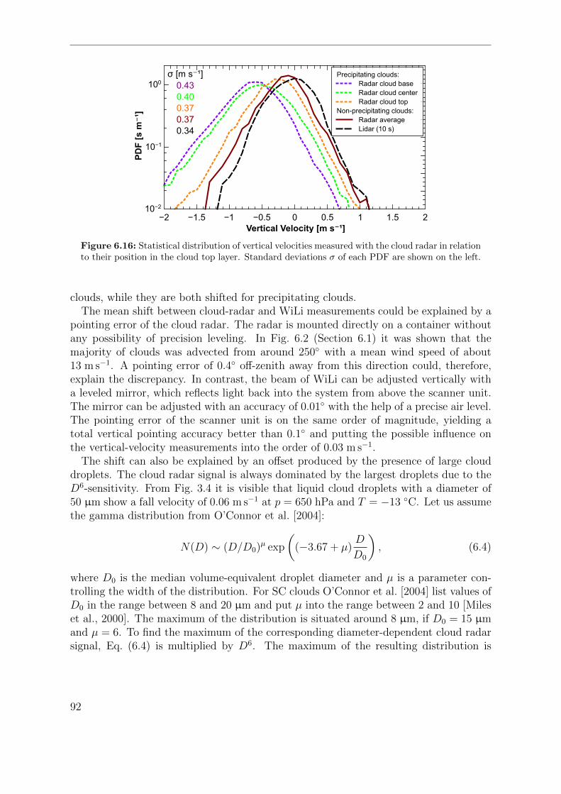
PD
F [
s m⁻¹
]
10−2
10−1
100
Vertical Velocity [m s⁻¹]−2 −1.5 −1 −0.5 0 0.5 1 1.5 2
Precipitating clouds: Radar cloud base Radar cloud center Radar cloud top
Non-precipitating clouds: Radar average Lidar (10 s)
Figure 6.16: Statistical distribution of vertical velocities measured with the cloud radar in relationto their position in the cloud top layer. Standard deviations σ of each PDF are shown on the left.
clouds, while they are both shifted for precipitating clouds.The mean shift between cloud-radar and WiLi measurements could be explained by a
pointing error of the cloud radar. The radar is mounted directly on a container withoutany possibility of precision leveling. In Fig. 6.2 (Section 6.1) it was shown that themajority of clouds was advected from around 250 with a mean wind speed of about13 m s−1. A pointing error of 0.4 off-zenith away from this direction could, therefore,explain the discrepancy. In contrast, the beam of WiLi can be adjusted vertically witha leveled mirror, which reflects light back into the system from above the scanner unit.The mirror can be adjusted with an accuracy of 0.01 with the help of a precise air level.The pointing error of the scanner unit is on the same order of magnitude, yielding atotal vertical pointing accuracy better than 0.1 and putting the possible influence onthe vertical-velocity measurements into the order of 0.03 m s−1.
The shift can also be explained by an offset produced by the presence of large clouddroplets. The cloud radar signal is always dominated by the largest droplets due to theD6-sensitivity. From Fig. 3.4 it is visible that liquid cloud droplets with a diameter of50 µm show a fall velocity of 0.06 m s−1 at p = 650 hPa and T = −13 C. Let us assumethe gamma distribution from O’Connor et al. [2004]:
N(D) ∼ (D/D0)µ exp
((−3.67 + µ)
D
D0
), (6.4)
where D0 is the median volume-equivalent droplet diameter and µ is a parameter con-trolling the width of the distribution. For SC clouds O’Connor et al. [2004] list values ofD0 in the range between 8 and 20 µm and put µ into the range between 2 and 10 [Mileset al., 2000]. The maximum of the distribution is situated around 8 µm, if D0 = 15 µmand µ = 6. To find the maximum of the corresponding diameter-dependent cloud radarsignal, Eq. (6.4) is multiplied by D6. The maximum of the resulting distribution is
92

6. Statistical properties of layered clouds
a)
v C
lou
d R
adar
[m
s⁻¹
]
−1
−0.5
0
0.5
1
v Doppler Lidar [m s⁻¹]−0.4 −0.2 0 0.2 0.4
precipitating non-precipitating f(x) = x
b)
v C
lou
d R
adar
90 [
m s⁻¹
]
0
0.5
1
1.5
v Doppler Lidar90 [m s⁻¹]0 0.5 1 1.5
precipitating a=0.7 (R²=0.2) non-precipitating a=1.05 (R²=0.5)
Figure 6.17: Scatterplots of vertical-velocity mean values (a) and 90% percentile of the updraftvelocities (b) for single cloud cases measured with cloud radar and WiLi. Only cases with morethan 150 valid vertical-velocity values from both instruments are considered. Slope values of alinear fit function f(x) = ax are shown.
now at 20 µm, corresponding to a terminal fall velocity of 0.01 m s−1. 95% of the radarsignal originates from particles smaller than D = 30 µm, which again corresponds toa terminal fall velocity of 0.04 m s−1. Taking into account turbulent air motion insideof the cloud layers, all velocity measurements would be distributed equally around thecentral velocity bin of the cloud radar and the vertical-velocity statistics should not beshifted by more than 0.04 m s−1. However, the production of a very small amount ofdrizzle droplets bigger than 30 µm could add to this. One droplet of 100 µm producesa signal which is a factor of 1006/306 = 1371 stronger than that of a droplet with adiameter of 30 µm and has already a fall speed of 0.4 m s−1 at 650 hPa (see Fig. 3.4).
6.5.3 Cloud-base vertical-velocity distribution as a function ofheight and temperature
Numeric climate and weather models usually do not resolve in-cloud turbulence directly.Hence, parameterizations are applied to describe the vertical movements in the atmo-sphere [Tonttila et al., 2013; West et al., 2013]. Measurements of vertical air velocity arethus required to either evaluate these parameterizations or to initialize the model (seeSection 2.4). A possible height or temperature dependence of cloud-base vertical veloc-ity is examined in Fig. 6.18a and 6.18b. Within this statistic, no significant differencesin the vertical motions are found for the considered temperature and height range. Theabsence of such a dependence has big advantages for modeling, because only a reducednumber of parameterizations is required. It can also be concluded that the physicalmechanism creating and maintaining the turbulence must be independent of height andtemperature.
93

a)
Vertical Velocity [m s⁻¹]
CT
H [k
m]
Rel
. Fre
quen
cy (
log
10)
-2.0 0.0 2.0-1.0 1.01
5
7
4
6
3
2
-1
-2
-3
-4
b)
Vertical Velocity [m s⁻¹]
CT
T [°
C]
Rel
. Fre
quen
cy (
log
10)
-2.0 0.0 2.0-1.0 1.0
-20
-30 -1
-2
-3
-4
-10
0
+10
Figure 6.18: Distribution of vertical velocities in dependence of cloud top height (a) and cloudtop temperature (b). All cloud cases from the UDINE dataset are taken into account, for whichWiLi data is available. Each row is normalized to its sum. Deviations at +3 and −25 C are dueto a lower number of cloud cases within this specific temperature interval.
6.5.4 Effects of solar forcing and cloud phase on vertical-velocitystatistics
Solar irradiation is one major driver of global air movements and can influence cloudsby radiative heating. In this section, the solar influence on mid-level layered cloudsis explored by sub-dividing the supercooled cloud cases of the UDINE dataset intoliquid/mixed-phase and daytime/night-time cases. As before, the decision between liq-uid and mixed-phase clouds was made according to the cloud classification scheme intro-duced in Section 4.5. Daytime and night-time cases are separated by a ±2-hour intervalaround sunset and sunrise, respectively. Cases overlapping with this interval are left outfrom the daytime/night-time decision. The analyzed dataset is restricted to supercooledclouds to investigate the connection between vertical-velocity distribution and ice for-mation. Warm clouds would introduce a bias, because they principally cannot form iceand would only randomly attribute vertical-velocity values to the liquid-cloud fraction.Therefore, a “liquid” cloud is also a non-precipitating cloud in this context.
For all possible combinations of the classifications Fig. 6.19 shows the vertical-velocitydistributions at cloud bases. The first to fourth statistical moments were derived foreach distribution and are shown in Table 6.1. The first moment is the mean value v,the second moment the variance σ2
v . The third moment of a sample with N values iscomputed by
γ3 = N−1
N∑i=1
(vi − vσv
)3
(6.5)
94

6. Statistical properties of layered clouds
Vertical Velocity [m s⁻¹]
Pro
babi
lity
Den
sity
Fun
ctio
ns [s
m⁻¹
]
liquid mixed-phase
night
day day & liquid day & mixed-phase
night & liquid night & mixed-phase
all cases
Dev
iatio
n fr
om m
ean
[%]
168 60 108
92 40 52
48 12 36
* **
Figure 6.19: Vertical-wind statistics for different types of supercooled cloud layers. In eachsub-figure the histogram of the total dataset is plotted as a reference (gray background) and thenumber of involved cloud cases is given in the upper left corner. See Table 6.1 for the moments ofeach PDF.
Table 6.1: Moments of the vertical-velocity distributions for different combinations of cloud phaseand time of appearance (see histograms in Fig. 6.19).
No. of cases Average Variance Skewness Kurtosis– m s−1 m2 s−2 – –
all 168 −0.068 0.210 −0.441 1.411mixed 108 −0.092 0.232 −0.426 1.220liquid 60 0.003 0.134 −0.113 1.086day 92 −0.034 0.204 −0.349 1.701
night 48 −0.109 0.189 −0.499 1.231day and mixed 52 −0.060 0.243 −0.322 1.361day and liquid 40 0.017 0.122 −0.018 1.087
night and mixed 36 −0.124 0.196 −0.479 1.169night and liquid 12 0.008 0.119 −0.283 0.877
95

and called skewness, the fourth moment is
γ4 =
N−1N∑i=1
(vi − v)4
(N−1N∑i=1
(vi − v)2)2
− 3 (6.6)
and called kurtosis. The third moment is a measure for the asymmetry of the distri-bution. The fourth moment indicates any excess of the distributions compared with aGaussian distribution. The third and the fourth moments are very sensitive towardsoutliers, therefore all moments are computed for the velocity range between −3 and3 m s−1. In this interval nearly all significant vertical-velocity values are located (seelogarithmic graph in Fig. 6.13a).
An influence of solar forcing may be visible from Fig. 6.19 in the graphs marked withday (orange) and night (blue). Compared with the mean dataset in the background(gray), the PDF of the day cases is about 50% larger at an updraft of 1 m s−1. Atthis vertical velocity, the PDF from the night cases is 50% smaller compared with themean dataset. This difference may be attributed to solar heating introducing moreenergy into the cloud. The mechanism leading to an increase in updraft strength might,however, not be straightforward. The main source of turbulent energy for layered cloudsis probably radiative cooling at cloud top. It is visible that the higher vertical velocitiesoccur mainly in mixed-phase clouds (category: day & mixed-phase in Fig. 6.19). Theinfluence of solar radiation on particle growth in mixed-phase clouds is discussed in Leboet al. [2008], where it is found that solar heating can, e.g., influence the effectiveness ofthe WBF process.
It is worth noting that the vertical-velocity distribution of liquid clouds shows a meanvalue (1st moment) of 0.003 m s−1 (see Table 6.1). Additionally, the skewness (3rdmoment) of the distribution is only −0.113, meaning that it is very close to the Gaussiandistribution. The influence of falling particles can, again, be seen between the right andthe middle column in Fig. 6.19. The excess at vertical velocities around −1.5 m s−1
is clearly more prominent in the mixed-phase cases. The mean shift towards negativevalues in these cases is probably due to the influence of falling particles. This effect isinvestigated in Section 6.5.6.
6.5.5 Comparison between sub-tropics and mid-latitudesLayered clouds in the sub-tropics and in mid-latitudes occur under very different me-teorological conditions. In mid-latitudes, they mainly follow frontal systems, in thesub-tropics the influence of gravity waves generated from deep convective systems maybe a more prominent driver. Figure 6.20 compares the statistical distributions of thefirst to fourth distribution moments retrieved from the single cases. It is visible thatthe overall statistical parameters of both datasets are very similar and no significantdifferences can be found for the first three moments. Only the fourth moment (kurto-sis), which describes an excess in the outer parts of the histogram, is considerably larger
96

6. Statistical properties of layered clouds
a) LeipzigVa
lues
−2
−1
0
1
2
Moment1st 2nd 3rd 4th
1st (Mean) [m s⁻¹]2nd (Variance) [m² s⁻²]3rd (Skewness)4th (Curtosis)
→ 4.2
b) Praia
Valu
es
−2
−1
0
1
2
Moment1st 2nd 3rd 4th
1st (Mean) [m s⁻¹]2nd (Variance) [m² s⁻²]3rd (Skewness)4th (Curtosis)
→ 3.8
Figure 6.20: Comparison of first to fourth statistical moments of the vertical velocities for allcloud cases recorded at Leipzig (a) and Praia (b). Large boxes indicate the 25% and 75% percentilesaround the mean values (circles), while the bars show the 5% and 95% percentiles.
a) Leipzig
Verti
cal V
eloc
ity [m
s⁻¹
]
−3
−2
−1
0
1
2
3
MAX MEAN MIN STD
b) Praia
Verti
cal V
eloc
ity [m
s⁻¹
]
−3
−2
−1
0
1
2
3
MAX MEAN MIN STD
MAXMEANMINSTD
→ -4.2
Figure 6.21: Comparison of the minimum (MIN), maximum (MAX), mean (MEAN) and standarddeviation (STD) of the vertical-velocity distributions recorded at Leipzig (a) and Praia (b). Thestatistics consist of the single values derived for each cloud case. Large boxes indicate the 25% and75% percentiles around the mean values (circles), while the bars show the 5% and 95% percentiles.
97

a)
PD
F [
s m⁻¹
]
10−3
10−2
10−1
100
Vertical Velocity [m s⁻¹]−2 −1 0 1 2
1st2nd3rd4th
0.0030.121
-0.0680.856
-0.0110.147
-0.7133.630
Leipzig liquid (2 s) Praia liquid (5 s) Leipzig liquid (6 s)
b)
PD
F [
s m⁻¹
]
10−3
10−2
10−1
100
Vertical Velocity [m s⁻¹]−2 −1 0 1 2
Leipzig mixed-phase (2 s) Praia mixed-phase (5 s) Leipzig mixed-phase (6 s)
1st2nd3rd4th
-0.0960.205
-0.3781.190
-0.0230.166
-0.9703.552
Figure 6.22: PDFs of the vertical velocities at cloud base measured with WiLi at Leipzig and atPraia for supercooled liquid (a) and mixed-phase cloud layers (b).
for the clouds at Praia. Hence, the distribution is deviating stronger from a Gaussianshape at high vertical velocities. Further distributions of maximum, minimum, meanand standard deviation are shown in Fig. 6.21. Before selection of the absolute mini-mum and maximum, a 3-bin median filter was applied on each cloud case to avoid noiseartifacts. Strongest differences can be found here in the maximum and minimum val-ues, which corresponds to the differences found in the kurtosis. The kurtosis increasesrapidly, if such outliers are present within the dataset. Differences are mainly visible inthe higher moments. This discrepancy probably results from a low amount of very highvertical-velocity values, measured at Praia. Occasional strong wave motion in the uppertroposphere could influence the vertical-velocity pattern in the sub-tropical clouds.
In Figure 6.22 the vertical velocities at cloud bases are compared for the datasetsfrom Leipzig (UDINE) and Praia (SAMUM-2). The values of UDINE were averaged ona 6-s timegrid to better compare to the 5-s timegrid used in the SAMUM-2 experiment.A further classification beyond mixed-phase and liquid clouds, as shown before, is notdone in this case, because the number of cases is not sufficient and the significanceof the statistics would be too low. Statistical moments are given in the figure. Forliquid clouds, both statistics are nearly identical. Significant differences show up onlyfor mixed-phase clouds at negative vertical-velocities. The right flanks of the vertical-velocity histograms from Leipzig and Praia are very similar in both cases. For liquidcases, PDF values agree within 5% in the range from −0.9 to 0.9 m s−1. That is anamazing result, given the fact that the two datasets were recorded about 5000 km and5 years apart. The updraft statistics in the panel shown in Fig. 6.19 and the height-and temperature-resolved histograms in Fig. 6.18a are also very similar. The physicalprocess behind the generation of these clouds, therefore, appears to be universal. Onceformed, layered clouds seem to be largely independent structures, kept alive by theirinternal motion.
98

6. Statistical properties of layered clouds
6.5.6 Investigation of the excess at negative vertical velocitiesIn the previous sections, it was shown that the statistics of vertical velocities at cloudbase can be easily derived for non-precipitating clouds (see Fig. 6.19 and 6.22). Forprecipitating clouds the derivation of meaningful statistical properties is more difficult,because falling particles partially mask the movements of the small cloud droplets atcloud base. Such effects can be seen, e.g., in Fig. 6.22b, where an excess at negativevertical velocities is visible. That excess may originate from downdraft regions withinthe cloud, where cloud droplets have dissolved and only the falling ice crystals are leftto produce a Doppler lidar signal. One can assume that the vertical air movements inthese areas of the cloud are statistically not different from the rest of the cloud.
In Fig. 6.23 it is, therefore, attempted to reproduce the statistics of mixed-phase cloudsfrom the statistics in pure liquid clouds. This approach is based on the assumption thatin mixed-phase cloud layers falling ice crystals, drizzle droplets and cloud droplets aresubject to the same turbulent motion. The vertical-velocity statistics of falling particlesis just offset by their fall velocity (see Fig. 6.16). The vertical-velocity statistics of mixed-phase clouds should, therefore, be reproducible from the statistics of non-precipitatingclouds by just adding up different shifted modes. It is visible from Fig. 6.23 that thestatistical distribution of mixed-phase clouds is matched closely assuming two additional
[s m⁻¹
]
10−3
10−2
10−1
100
Vertical Velocity [m s⁻¹]−2 −1.5 −1 −0.5 0 0.5 1 1.5 2
Mixed Phase Liquid 3-Mode Composite
Figure 6.23: The histogram of vertical velocties at the base of liquid clouds at Leipzig (blue curve)is used to reproduce the same statistics in mixed-phase clouds (red curve) assuming additionalmodes resulting from falling particles (green vertical lines). At the position of the green verticalbars, the blue curve is added with the corresponding weightings of the bars, which are 1.0 forthe droplet mode at 0 m s−1, 0.4 for the first falling particle mode at −0.3 m s−1 and 0.06 for thethird particle mode at −1.2 m s−1. The resulting distribution is renormalized and displayed as thedashed green line.
99

modes of falling particles. This finding finally explains the excess at negative velocityas particle-influenced and indicates that the velocity distribution is similar even forprecipitating mixed-phase clouds and non-precipitating liquid clouds. It is also visiblefrom Fig. 6.23 that the influence of falling-particle modes on the right flank (updrafts)of the PDF is limited.
100

7 Towards the measurement ofice-particle flux from cloud-radarspectra
In the previous chapters, it has been shown what new and exciting synergistic effectsshow up, when combining different velocity-resolving instruments. Especially Dopplerlidar and cloud radar were found to perform well together, but also the addition of a windprofiler showed that this combination of instruments has a lot of uncharted potential. Aprecise and unbiased measurement of vertical velocity makes it, e.g., possible to directlyderive information about size and shape of particles. However, it is extremely difficultto observe processes within the top layer of the cloud, because liquid droplets and icecrystals coexist in the observation volume and are in turbulent motion. The processeswithin the cloud layer itself, which are vital for the understanding of heterogeneous iceformation, are therefore hidden.
In this chapter, an approach is described to detect and quantify heterogeneous icenucleation at cloud top. A combination of Doppler lidar, cloud radar and wind profileris used to capture the vertical motions at cloud base and inside a mixed-phase cloud layerand to separate liquid droplets and ice crystals by their fall velocities. A major problemis the strong turbulence within the mixed-phase layers, which distorts the cloud-radarspectra. The turbulent and instrumental distortions of the radar spectra are thereforemeasured with the help of a wind profiler and/or a Doppler lidar. Subsequently, thedetected distortions are removed with the help of a deconvolution technique, similarto the one introduced in Section 5.1. The velocity scale of the spectra can then bedirectly converted to particle sizes, using the approach of Heymsfield and Westbrook[2010] presented in Section 3.2.4.
In Section 7.1, it is shown that the process of ice nucleation can be sensed remotely,if the flux of ice particles through the cloud base can be quantified. A way towards thederivation of the particle flux from cloud-radar spectra is explained in Section 7.2. A de-convolution method to correct distorted cloud-radar spectra is presented in Section 7.3.Treated spectra are used in Section 7.4 to derive microphysical information about thefalling particles. The retrieval of the particle size distribution is attempted directly fromthe reconstructed cloud-radar spectra, using information from multiple measurementsystems to remove disturbances and shifts introduced by vertical motion. Measure-ment uncertainties and potential further developments of the method are discussed inSection 7.6.
Vertical-velocity information has already been used before in the study of high clouds
101

[Matrosov et al., 2002; Mace et al., 2002; Deng and Mace, 2006, 2008]. Heymsfield andIaquinta [2000] employed such a method to gain insight into the climatology of cirrusclouds and particle transport mechanisms. A first application to low clouds was done bySeifert et al. [2012]. Westbrook et al. [2007] and Luke and Kollias [2013] presented meth-ods to separate cloud droplets and drizzle. The aforementioned methods use moments,derived from radar spectra, thereby assuming a certain size or velocity distribution.Protat and Williams [2011] used a combination of a 3-GHz Doppler radar and a 50-MHz wind-profiler to validate statistical relationships between terminal fall velocity andradar signal, but left the size information implicit. Recently, Westbrook and Illingworth[2013] measured particle flux with aircraft within an arctic mixed-phase cloud layer.The method presented here is solely based on ground-based remote-sensing techniquesand does not make any assumptions on particle size distribution. All information isretrieved directly from corrected cloud-radar spectra. The synthesis of measurementsfrom Doppler lidar, cloud radar and wind profiler on the scales of single measurementvolumes has never been done before. In the context of this work, it is shown thatthis combination of instruments can provide crucial information to approach the remotesensing of ice nucleation. The method must, however, not stand apart from the othermethods mentioned above. It can be used with any of them, by just delivering treatedradar spectra to them to improve the quality of the input data.
7.1 A measure for the particle nucleation rateaccessible by remote sensing
It has been shown before that ice particles and water droplets can be observed byboth lidars and radars. However, it is extremely difficult to observe the process ofice nucleation itself, i.e., the moment when a water droplet turns into an ice particle.This process is therefore mainly studied in laboratories [Phillips et al., 2013], wherethe number of supercooled droplets can be controlled and the generated ice crystalscan be studied in situ. Unfortunately, experimental validation of such experiments innature is largely missing. This lack of data is mainly due to the fact that the process ishidden inside the mixed-phase cloud top layer and unaccessible by established remote-sensing methods. It is already difficult to even find an observable parameter that isuseful to quantify the process of ice nucleation. Fig. 7.1 illustrates this problem byshowing two scenarios, in which ice particles are generated from liquid-water dropletswithin the cloud top layer. They subsequently begin to fall through the layer, until theyappear at cloud base. The sketch makes clear, why it is not enough to measure particlenumber concentration alone. The number concentrations of ice particles directly belowcloud base differ by a factor of five between the two scenarios, but the flux F = N × vof particles is equally 1 m−2 s−1 in both cases. Hence, the rate of ice production in thecloud top layer is the same, but in the second case particle growth and deposition happenfaster.
When the particle number concentration can be measured together with the terminal
102

7. Measuring ice-particle flux
ice particles:D = 1500 µmN = 1 m⁻³v = 1.0 m s⁻¹mtotal = 80 µg
ice particles:D = 400 µmN = 5 m⁻³v = 0.2 m s⁻¹mtotal = 15 µg
liquid droplets:D = 30 µmN = 108 m⁻³v = 0.0 m s⁻¹mtotal = 1.5 g 1m³
a) b)
Figure 7.1: Illustration of the difficulties occurring in quantification of heterogeneous ice forma-tion.
fall velocities, the total particle flux F =∫N(D)v(D) dD can be calculated. F indicates
the number of particles leaving the cloud base in each second, a quantity that is directlylinked to the number of particles generated within the cloud top layer in each second. Itis important to catch the particles directly at cloud base at the latest, because furtherdownwards in the virga they are altered, e.g., by evaporation processes and consequentlytheir number and shape is changed. It is even more important, although extremelydifficult, to separate the ice and water particles within the liquid cloud layer, to restrictthe location where ice nucleation happens.
It has been demonstrated in Chapter 3 that the MIRA-35 cloud radar can detectparticle number concentrations of about 1 m−3, if Dm ≈ 300 µm. Recently, it has beenshown by Schmidt et al. [2013] that the number concentration of liquid droplets in alayered cloud can be measured with a dual-field-of-view (DFOV) Raman lidar. In ACcloud layers, droplet number concentrations of 108 m−3 were found with that technique[Schmidt et al., 2014]. Consequently, ratios between ice and water particles on the orderof 10−8 can be measured with a combined lidar/radar approach. The particle flux andthe particle nucleation rate would be on the same order of magnitude, if particle fallvelocities of approximately 0.5 m s−1 to 1.0 m s−1 are assumed. Currently, there is noexperimental method available that can measure such low particle nucleation rates inreasonable time, motivating further efforts into this direction.
103

7.2 Deriving ice-particle flux from cloud-radar spectraThe cloud radar collects the backscatter signal of all particles moving with the samevelocity in one spectral bin. The velocity of the n-th bin is v(n) = n∆v (with n =−128...128). (Even though a discrete quantity, the velocity scale of the cloud radaris denoted in the form v(n) to avoid misunderstandings with other indices introducedbefore). For this work, the MIRA-35 cloud radars of LACROS and MOL were run with∆v = 0.08 m s−1. If any spectral broadening has been corrected, vt(n) = −(v(n)− uz)(with uz the mean vertical velocity of air in the cloud radar observation volume dur-ing integration time) represents the terminal fall velocity relative to the surroundingair. The connection between terminal fall velocity and the maximum diameter Dm hasbeen explored in Section 3.2.4. A monotonically increasing and steady function vt(Dm)(Eq. (3.24)) can be inverted numerically to derive Dm(vt(n)) = Dm(n) and, consequently,
0
Z(n) [dBZ]
v(n) [cm s⁻¹]-8-16-24-32-40-48-56... 5648403224168 ...
Zth
0
N(n) [m⁻³]
Dm(n) [µm]
100
200
300
400
500
600
...
700
800
900
potentially undetected small particles
potentially undetected big particles
1) Radar Spectrum 3) Retrieved Size Spectrum
Dm [µm]
vt [cm s⁻¹]
Zi
N=Z/(K²D⁶)
falling particles mean vertical velocity
of air (uz)
cloud droplets
08162432404856... 6472
2) vt-Dm Parameterization
Figure 7.2: Overview about the proposed scheme to derive number concentration from cloud-radarspectra and measured terminal fall velocity v. It is assumed that all turbulence and instrumentaleffects are removed from the spectrum and only the vertical-velocity bias is left. In this examplean updraft of 0.24 m s−1 is shifting the spectrum towards larger vertical velocities. If the verticalvelocity of air is known, the size of the particles can be estimated from vt = −(v − uz).
104

7. Measuring ice-particle flux
Ap(Dm) and mp(Dm) of the particles.The spectral bin n of the cloud radar contains particles with the radar scattering cross
section
η(n) = N(n)4πsR180(mp(Dm(n))), (7.1)
assuming a signal from only one particle type within the bin. Rearranging for N(n) andinserting Eq. (3.10) yields
N(n) =π2ρ2
w,iZ(n)
36K2w,im
2p(Dm(n))
. (7.2)
Other observable parameters like particle flux
F =∑n
N(n)v(n), (7.3)
optical particle extinction coefficient
α =∑n
2N(n)Ap(n) (7.4)
andIWC =
∑n
mp(n) (7.5)
(where n must only run over bins, where ice is present) can be calculated from thesize spectrum with the known particle properties. For the calculation of F , it is of greatadvantage to have the information about number concentration and terminal fall-velocityon the same grid.
7.3 Preparation of cloud-radar spectraMeasuring the particle flux F calls for precise knowledge of the particle size distributiontogether with the spectral distribution of fall velocities. The velocity-resolved spectra ofthe MIRA-35 cloud radar do not directly represent the particles’ terminal fall velocities.The velocity scale is shifted by mean vertical movements and broadened by a varietyof phenomena occurring in the observation volume. There are several factors distortingthe true vertical-velocity spectrum:
• Sub-scale turbulence σ2t broadens the spectrum of any radar system, because of
turbulent motion on scales smaller than the observation volume.
• Particles at the edge of any radar observation volume are observed under a small
105

angle. This effect introduces the variance
σ2b =
u2aφ
2
2.76, (7.6)
with opening angle φ of the radar system and the advection speed ua [Shupe et al.,2008] and is called beam-width broadening.
• During data processing, an FFT window is applied to reduce noise. Consequently,an additional distortion is introduced into the spectrum. This broadening is smallcompared with the other ones, but it has a non-Gaussian shape and must, therefore,be treated separately.
• Shupe et al. [2008] also list broadening due to wind shear, but consider it lessimportant. Therefore, it is neglected here.
Unfortunately, the cloud radar needs a relatively long integration time to reduce elec-tronic noise. With increasing integration time, however, the contamination of the radarspectra by the above-mentioned effects increases. Thus, any broadening effects andshifts have to be removed before any method relating microphysical properties of parti-cles to their fall velocity can be applied to the cloud-radar spectra. The measurementand correction of the velocity scale is done by subtracting the mean vertical velocity ofair as demonstrated in Section 5.5.1.2. The reconstruction of the true spectral velocitydistribution is more difficult [e.g., Westbrook et al., 2007; Luke and Kollias, 2013]. If themechanisms that have broadened the spectrum are known, a deconvolution like in Sec-tion 5.1 can be applied. The PSF responsible for the broadening has to be constructedfrom the different broadening mechanisms. One approach is to represent the spread bybeam-width broadening (σb) and turbulence broadening (σt) by a Gaussian distribution
PSFbt(vn) =(σbt√
2π)−1
exp
[−0.5
(vnσbt
)2], (7.7)
with the variance σ2bt = σ2
b + σ2t . The PSF of the FFT window can be calculated
analytically by Fourier transforming the window (in this case a Hann window). Toacquire the total PSF, both functions are numerically convolved on the grid of the radarspectra and normalized in such a way that the sum of all points is 1. This normalizationis necessary to conserve the total signal of the treated cloud-radar spectra. Fig. 7.3 showsan example PSF, which assumes σb = 0.4 and σt = 0.3. In the approach presented here,information about broadening and shifts that contamined the measured velocity spectraare collected by Doppler lidar and wind profiler, measuring simultaneously with thecloud radar.
The RL algorithm is very sensitive towards deviations in the PSF, which is desired,because artifacts can be identified easily. If the assumed PSF is not correct, the deconvo-lution instantly fails or produces unrealistic results with the test function strongly devi-ating from the original signal. In this context, the compressed spectra of the cloud radar
106
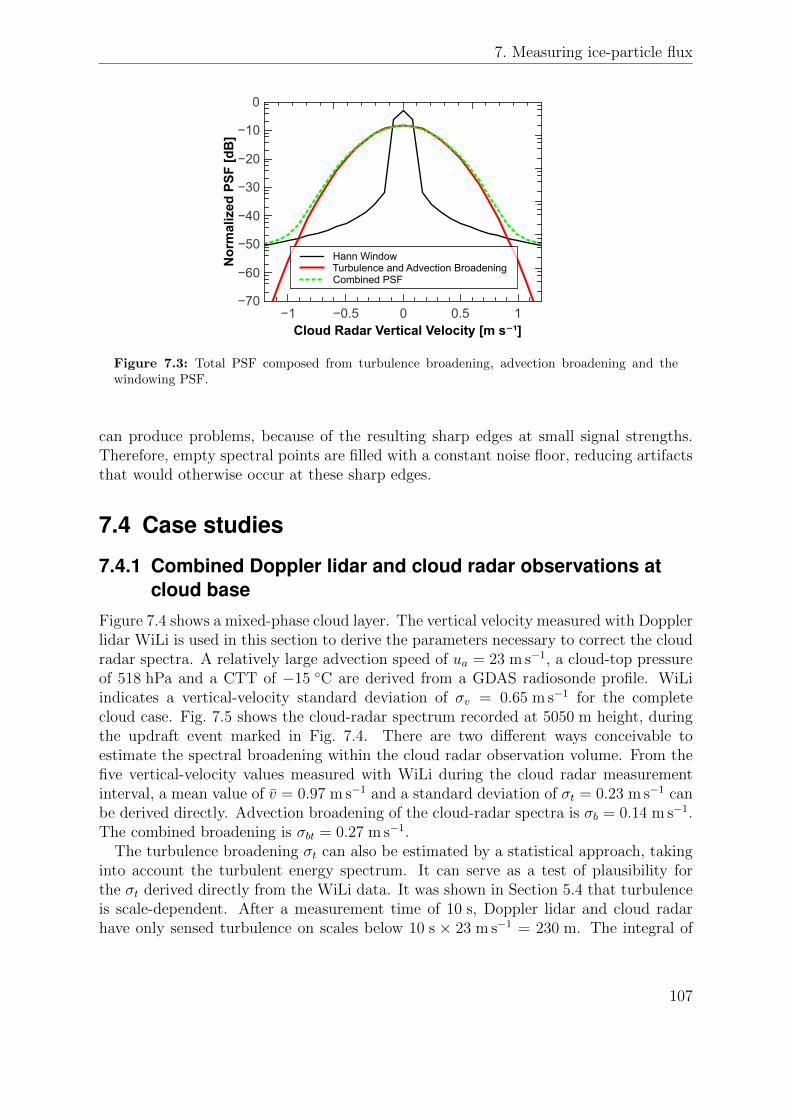
7. Measuring ice-particle flux
Nor
mal
ized
PSF
[dB
]
−70
−60
−50
−40
−30
−20
−10
0
Cloud Radar Vertical Velocity [m s⁻¹]−1 −0.5 0 0.5 1
234
Hann Window Turbulence and Advection Broadening Combined PSF
Figure 7.3: Total PSF composed from turbulence broadening, advection broadening and thewindowing PSF.
can produce problems, because of the resulting sharp edges at small signal strengths.Therefore, empty spectral points are filled with a constant noise floor, reducing artifactsthat would otherwise occur at these sharp edges.
7.4 Case studies
7.4.1 Combined Doppler lidar and cloud radar observations atcloud base
Figure 7.4 shows a mixed-phase cloud layer. The vertical velocity measured with Dopplerlidar WiLi is used in this section to derive the parameters necessary to correct the cloudradar spectra. A relatively large advection speed of ua = 23 m s−1, a cloud-top pressureof 518 hPa and a CTT of −15 C are derived from a GDAS radiosonde profile. WiLiindicates a vertical-velocity standard deviation of σv = 0.65 m s−1 for the completecloud case. Fig. 7.5 shows the cloud-radar spectrum recorded at 5050 m height, duringthe updraft event marked in Fig. 7.4. There are two different ways conceivable toestimate the spectral broadening within the cloud radar observation volume. From thefive vertical-velocity values measured with WiLi during the cloud radar measurementinterval, a mean value of v = 0.97 m s−1 and a standard deviation of σt = 0.23 m s−1 canbe derived directly. Advection broadening of the cloud-radar spectra is σb = 0.14 m s−1.The combined broadening is σbt = 0.27 m s−1.
The turbulence broadening σt can also be estimated by a statistical approach, takinginto account the turbulent energy spectrum. It can serve as a test of plausibility forthe σt derived directly from the WiLi data. It was shown in Section 5.4 that turbulenceis scale-dependent. After a measurement time of 10 s, Doppler lidar and cloud radarhave only sensed turbulence on scales below 10 s × 23 m s−1 = 230 m. The integral of
107

Hei
ght [
m]
Hei
ght [
m]
Ver
tical
Vel
ocity
[m s
⁻¹]
Ver
tical
Vel
ocity
[m s
⁻¹]
Doppler Lidar WiLi
Cloud Radar
Cloud RadarDoppler Lidar WiLi
Ver
tical
Vel
ocity
[m s
⁻¹]
Figure 7.4: Vertical velocity at the cloud base (WiLi) and particle fall velocity (cloud radar). Atthe height of the black arrows, the cloud-radar spectrum and the mean vertical velocity from WiLiare extracted for the following analysis (see Fig. 7.5). The cloud layer was recorded at Leipzig on17 September 2012.
the turbulent energy spectrum from k = 2π230 m
= 0.026 m−1 to the end of the spectrumyields σt = 0.20 m s−1, leading to a combined spectral broadening of σbt = 0.24 m s−1.Hence, the values for σbt from the direct and the statistical approach correspond within12%.
The cloud-radar spectrum can be successfully deconvolved with both values. InFig. 7.5, σbt = 0.24 m s−1 is used. The quality of the deconvolution is assured by thetest function, which is the convolution of the deconvolved data with the PSF. It isdrawn in green in Fig. 7.5 and corresponds well with the original cloud-radar spectrum(R2 > 0.997). For the updraft event, a mode of presumably liquid particles becomesvisible around the mean vertical-velocity measured with WiLi. The resulting spectrummay not yet be a perfect representation of the undisturbed cloud-radar spectrum, dueto the uncertainties in the assumed PSF, but different peaks are visible now.
The example demonstrates that it is possible to separate different particle modes
108
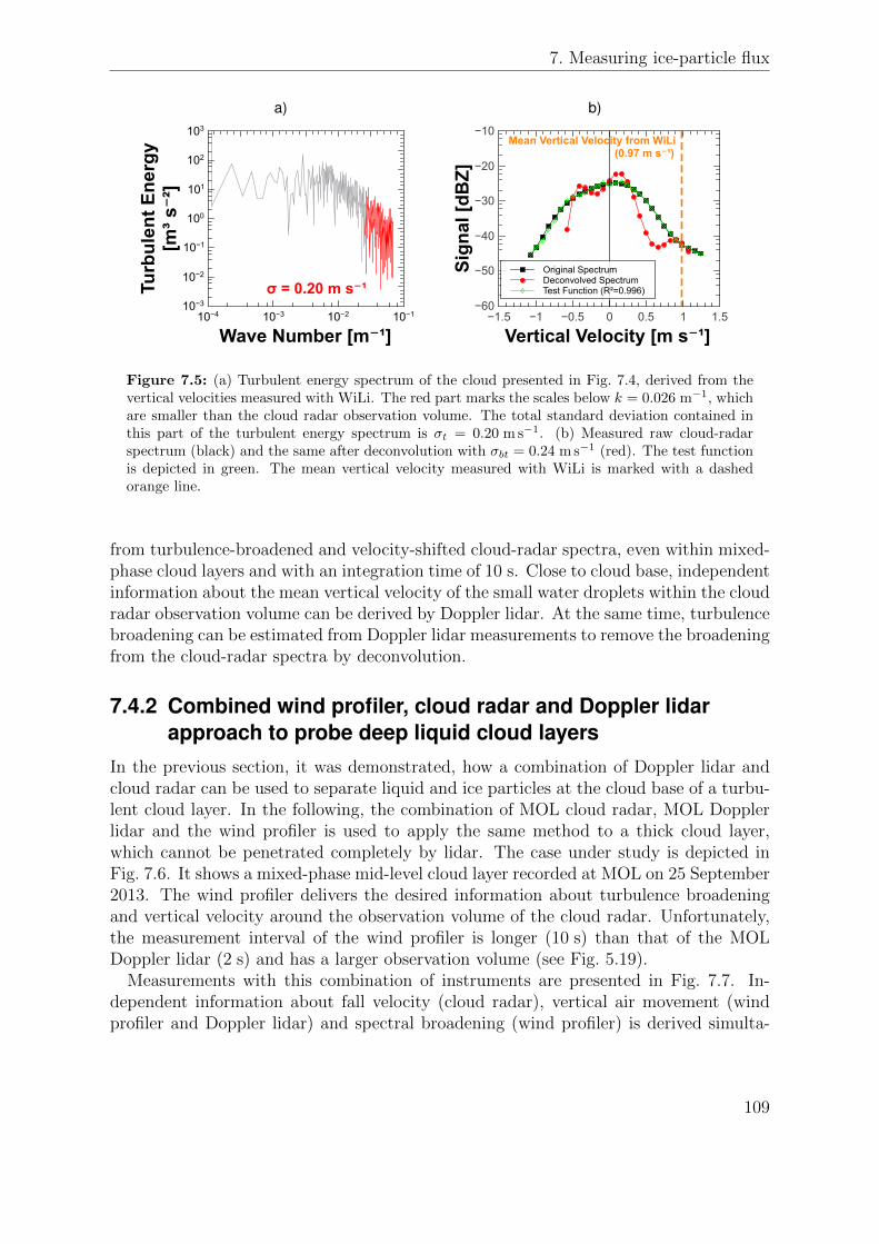
7. Measuring ice-particle flux
a)
Turb
ulen
t Ene
rgy
[m³ s⁻²
]
10−3
10−2
10−1
100
101
102
103
Wave Number [m⁻¹]10−4 10−3 10−2 10−1
σ = 0.20 m s⁻¹
b)
Sign
al [d
BZ]
−60
−50
−40
−30
−20
−10
Vertical Velocity [m s⁻¹]−1.5 −1 −0.5 0 0.5 1 1.5
Original Spectrum Deconvolved Spectrum Test Function (R²=0.996)
Mean Vertical Velocity from WiLi (0.97 m s⁻¹)
Figure 7.5: (a) Turbulent energy spectrum of the cloud presented in Fig. 7.4, derived from thevertical velocities measured with WiLi. The red part marks the scales below k = 0.026 m−1, whichare smaller than the cloud radar observation volume. The total standard deviation contained inthis part of the turbulent energy spectrum is σt = 0.20 m s−1. (b) Measured raw cloud-radarspectrum (black) and the same after deconvolution with σbt = 0.24 m s−1 (red). The test functionis depicted in green. The mean vertical velocity measured with WiLi is marked with a dashedorange line.
from turbulence-broadened and velocity-shifted cloud-radar spectra, even within mixed-phase cloud layers and with an integration time of 10 s. Close to cloud base, independentinformation about the mean vertical velocity of the small water droplets within the cloudradar observation volume can be derived by Doppler lidar. At the same time, turbulencebroadening can be estimated from Doppler lidar measurements to remove the broadeningfrom the cloud-radar spectra by deconvolution.
7.4.2 Combined wind profiler, cloud radar and Doppler lidarapproach to probe deep liquid cloud layers
In the previous section, it was demonstrated, how a combination of Doppler lidar andcloud radar can be used to separate liquid and ice particles at the cloud base of a turbu-lent cloud layer. In the following, the combination of MOL cloud radar, MOL Dopplerlidar and the wind profiler is used to apply the same method to a thick cloud layer,which cannot be penetrated completely by lidar. The case under study is depicted inFig. 7.6. It shows a mixed-phase mid-level cloud layer recorded at MOL on 25 September2013. The wind profiler delivers the desired information about turbulence broadeningand vertical velocity around the observation volume of the cloud radar. Unfortunately,the measurement interval of the wind profiler is longer (10 s) than that of the MOLDoppler lidar (2 s) and has a larger observation volume (see Fig. 5.19).
Measurements with this combination of instruments are presented in Fig. 7.7. In-dependent information about fall velocity (cloud radar), vertical air movement (windprofiler and Doppler lidar) and spectral broadening (wind profiler) is derived simulta-
109

Ver
tical
Vel
ocity
[m s⁻¹
]
Hei
ght [
m]
MOL Cloud Radar
Rad
ar R
efl.
Fac
tor
[dB
Z]
MOL Cloud Radar (Vertical Velocity)
Wind Profiler (Vertical Velocity)
MOL Doppler Lidar (Vertical Velocity)
Figure 7.6: Combined measurement with vertically looking MOL cloud radar, wind profiler andMOL Doppler lidar at MOL on 25 September 2013.
Wind ProfilerSpectral Width [m s⁻¹]
MOL Doppler lidarVertical Velocity [m s⁻¹]
Wind ProfilerVertical Velocity [m s⁻¹]
MOL Cloud RadarVertical Velocity [m s⁻¹]
Hei
ght [
m]
Figure 7.7: Extract from black box in Fig. 7.6 to give a detailed look into the vertical velocityand spectral width measured with MOL Doppler lidar, MOL cloud radar and wind profiler. Thecrosses indicate the positions of the spectra in Fig. 7.9 and 7.10.
110

7. Measuring ice-particle flux
Vert
ical
Vel
ocity
and
Spec
tral
Wid
th [m
s⁻¹
]
−1
−0.5
0
0.5
1
Rad
ar R
efle
ctiv
ity F
acto
r(C
loud
Rad
ar) [
dBZ]
−50
−40
−30
−20
−10
Height [km]2.0 2.5 3.0 3.5 4.0 4.5 5.0
224
Wind Profiler Vertical Velocity Wind Profiler Spectral Width Cloud Radar Signal
Figure 7.8: Profiles of wind profiler spectral width with correction for advection broadening (red),wind profiler vertical velocity (black) and radar reflectivity factor from cloud radar (dashed green)from Fig. 7.7 at 11:21 UTC.
neously. Fig. 7.8 shows profiles of vertical air velocity (black line) and spectral width(red line) from the wind profiler combined with the signal strength of the cloud radar(green line). A profile at 11:21 UTC is depicted. The opening angle of the wind profileris 3.0 and with the help of a GDAS radiosonde profile the advection speed is estimatedto ua = 3.0 m s−1. Fig. 7.8 shows that the spectral width from the wind profiler is notinfluenced by big particles detected by the cloud radar. Above 5.0 km height, a drop isvisible in the the signal of the cloud radar, but the wind profiler continues to show aspectral width of about 0.7 m s−1, indicating turbulence as the reason for the spectralbroadening. At 4.0 km height, a spectral width of 0.6 m s−1 is measured. The mean 10-sstandard deviation of the vertical velocity measured with Doppler lidar is also about0.6 m s−1 within the turbulent layer at 4.0 km height.
Figures 7.9 and 7.10 show the cloud-radar spectra and the retrieved particle propertiesfrom the points marked in Fig. 7.7 with a black and a red cross, respectively. At theheight where the black cross is located, the wind profiler shows an average spectralwidth of w = 0.85 m s−1, strongly varying over the time interval depicted in Fig. 7.7.From the spectral width w, the turbulence component can be estimated to be σt =√
(w/2.4)2 − 0.142 = 0.36 m s−1, assuming a Gaussian peak and correcting for the beam-width broadening of the wind profiler of 0.14 m s−1. The beam-width broadening of theMOL cloud radar is σb ≈ 0.02 m s−1, which has neglible influence on the resulting σbt =0.36 m s−1. For this combined broadening, the deconvolution fails with the test functionstrongly deviating from the original spectrum (R2 = 0.80). A successful deconvolutionis possible up to σbt = 0.2 m s−1 as shown in Fig. 7.9a. In this figure, one peak around0.3 m s−1 vertical velocity and another separated peak around −0.6 m s−1 are revealed.There may be a third peak close to 0.0 m s−1. The reconstruction of a size distributionwith Eq. (7.2) from the deconvolved cloud-radar spectrum is shown in Fig. 7.9b. Themean vertical velocity (orange dashed line in Fig. 7.9a) was applied to estimate thepure terminal fall velocities of the particles relative to the surrounding air. A mode of
111

a)
Sign
al [d
BZ]
−60
−50
−40
−30
−20
−10
Vertical Velocity [m s⁻¹]−1.5 −1 −0.5 0 0.5 1 1.5
Original Spectrum Deconvolved Spectrum Test Function (R²=0.997)
Mean Vertical Velocity from Wind Profiler (0.26 m s⁻¹)
b)
Num
ber C
onc.
[m⁻³
]
10−4
10−2
100
102
104
106
Particle Max. Diameter [m]10−4 10−3
First Mode (realistic) Second Mode (diverging) Noise Floor
Figure 7.9: a) Raw radar spectrum (black line) and deconvolved one (red line) for the positionof the black cross in Fig. 7.8. b) Number concentrations derived from the deconvolved spectrum,assuming that only hexagonal columns are present.
a)
Sign
al [d
BZ]
−60
−50
−40
−30
−20
−10
Vertical Velocity [m s⁻¹]−1.5 −1 −0.5 0 0.5
Mean Vertical Velocity from Wind Profiler (0.17 m s⁻¹)
Original Spectrum Deconvolved Spectrum Test Function (R²=0.993)
b)
Num
ber C
onc.
[m⁻³
]
10−3
10−2
10−1
100
101
102
103
Particle Max. Diameter [m]10−4 10−3 10−2
Hexagonal Columns Aggregates of Side Planes
α = 4.7 Mm-1
IWC = 1.3×10⁻⁶ kg m-3
N = 413 m-3
α = 1.8 Mm-1
IWC = 1.2×10⁻⁷ kg m-3
N = 4 m-3
Figure 7.10: Same as Fig. 7.9, but for the position of the red cross in Fig. 7.7. The total signalin the cloud-radar spectrum is −24 dBZ. The retrieval of particle number concentration wasdone in (b) for two different particle parameterizations. The noise floors are indicated for bothsize distributions with dashed lines. The range of validity for aggregates of side planes is 600 to4100 µm, the resulting size distribution for this particle type is slightly outside this range.
112

7. Measuring ice-particle flux
large particles is reconstructed around Dm ≈ 1 mm. Thus, it remains unclear, if thoseparticles are large ice crystals or perhaps drizzle droplets. The signal strength of theradar is too low to measure a meaningful depolarization signal, and particles disappearbefore crossing the height of T = 0 C. The second peak diverges at smaller particlesizes, because it reaches up to positive vertical velocities.
Fig. 7.10a shows the same procedure applied to the point indicated by the red cross.At this height, the wind profiler shows a spectral width of 0.50 m s−1, also stronglyvarying between single profiles. From that value, σbt = 0.15 m s−1 is calculated. Thecloud-radar spectrum is successfully deconvolved with σbt = 0.1 m s−1 (R2 = 0.993). Theretrieved particle spectrum is shown in Fig. 7.10b for the two different particle typeshexagonal columns and aggregates of side planes. It is visible from Fig. 3.4 that thesetwo particle types represent two extreme possibilities exhibiting significantly differentfall velocities for the same particle maximum diameter.
The retrieved size distribution is tested using the method of Hogan et al. [2006].At 3800 m height (red cross) the radar reflectivity measured with the cloud radar is−24 dBZ, and a temperature of −8 C was derived from a GDAS radiosonde profile.With these values Eq. (6.1) yields α = 28± 14 Mm−1, and from Eq. (6.2) IWC =(7.3± 3.7)× 10−7 kg m−3 is derived. α and IWC derived from the spectra by Eqs. (7.4)and (7.5) are shown in Fig. 7.10b. For hexagonal columns, α and IWC are one order ofmagnitude too low. For aggregates of side planes, IWC is 50% too high and α is alsoone order of magnitude too low.
The derived IWC values for aggregates of side planes are within the uncertainty givenby Hogan et al. [2006]. The reasons for deviations in the other values can be manifold.Hogan et al. [2006] use the mean of the vertical and horizontal dimension Dvh of anice crystal to calculate particle properties and a mass and area parameterization, wheremp ∼ D1.9
vh and Ap ∼ D1.6vh . This procedure makes a direct comparison difficult. Also, an
additional mode of small crystals is attached to the measured spectrum at low crystalsizes, where the optical particle imager is no longer sensitive. Those particles couldalso be missed by the cloud radar. Unfortunately, no powerful lidar was available atMOL at the time of the measurements, so no independent verification of the opticalextinction values could be acquired. In future, comparison with methods like the oneproposed by Tinel et al. [2005] will probably be possible. The following calculationsuse the parameterizations for hexagonal columns, keeping in mind that the numberconcentrations might be different for other particle types.
Fig. 7.11 shows particle number concentration N and particle flux F derived from allcloud-radar spectra in the time-height interval from 11:07 to 11:56 UTC and 2000 to4500 m, indicated as a red rectangle in Fig. 7.6. Vertical-velocity values from the windprofiler are used to automatically correct the velocity scale of the cloud-radar spectra,so that it resembles the terminal fall velocity relative to the surrounding air. F andN in Fig. 7.11 are calculated from uncorrected and corrected terminal fall velocities.The imprint of the vertical air velocity is visible in the uncorrected values (left column).The fingerprint of the vertical air velocity is easily visible in the uncorrected spectra asan increase in number concentrations in updrafts and a decrease in downdrafts. Thiseffect is significantly reduced by subtracting the vertical air velocity measured with wind
113

Hei
gh
t [m
]
2000
2500
3000
3500
4000
4500
Ver
tica
l Vel
oci
ty [
m s⁻¹
]
−2
−1
0
1
2
Time from Start [s]11:07 11:23 11:40 11:56
Hei
gh
t [m
]
2000
2500
3000
3500
4000
4500
Ver
tica
l Vel
oci
ty [
m s⁻¹
]
−2
−1
0
1
2
Time from Start [s]11:07 11:23 11:40 11:56
Hei
gh
t [m
]
2000
2500
3000
3500
4000
4500
Nu
mb
er C
on
cen
trat
ion
[m⁻³
]
0.1
1
10
100
1000
11:07 11:23 11:40 11:56
Hei
gh
t [m
]
2000
2500
3000
3500
4000
4500
Par
ticl
e F
lux
[m⁻²
s⁻¹
]
0.1
1
10
100
1000
Time [UTC]
11:07 11:23 11:40 11:56
Hei
gh
t [m
]
2000
2500
3000
3500
4000
4500
Par
ticl
e F
lux
[m⁻²
s⁻¹
]
0.1
1
10
100
1000
11:07 11:23 11:40 11:56
Hei
gh
t [m
]
2000
2500
3000
3500
4000
4500
Nu
mb
er C
on
cen
trat
ion
[m⁻³
]
0.1
1
10
100
1000
11:07 11:23 11:40 11:56
no vertical velocity correction vertical-velocity correction with wind profiler
Wind Profiler(Vertical Air Velocity)
subtract
Time [UTC]
Time [UTC]
Time [UTC]
Cloud Radar(Full Spectra)
Figure 7.11: Comparison between the particle number concentration and particle flux retrievedwith the deconvolution method for uncorrected (left blue box) and corrected (right red box)terminal-fall-velocity fields. Values are derived for hexagonal columns. The presented time-heightsection is marked in Fig. 7.6 with a red box.
114

7. Measuring ice-particle flux
profiler from the cloud-radar vertical velocity and is best visible in the area markedwith a pink box. After correcting the vertical-velocity scale with the help of the windprofiler, coherent fall streaks become visible. The flux retrieved in this way refers tothe movement of the particles relative to the surrounding air and is, therefore, onlyproportional to particle properties.
The width of the wind-profiler spectra is unfortunately not only connected with thestrength of the turbulence and can be influenced by other factors like Rayleigh scatteringfrom particles and strong signal gradients. It can be used for demonstration purposes(like in Fig. 7.7), but a use for automated deconvolution is more complicated. Therefore,the correction of broadening by deconvolution is kept simple and is run with a fixedσbt = 0.1 m s−1. Hence, the effect of this correction cannot reach its full potentialin this example. The correction of the mean vertical velocity is far simpler and canbe done automatically on the complete dataset. Also automatic peak separation forspectra in Fig. 7.9 is not yet implemented. Therefore, the method usually diverges,when a liquid-water mode is present and the cloud-radar spectra show signals at v > 0.The algorithm then produces unrealistically high number concentrations, as it was seenbefore in Fig. 7.9b.
7.5 Size separation of particlesIn Fig. 7.12 the same measurement as in Fig. 7.11 is shown. In this figure, however, smalland big particles are shown separately. This presentation efficiently removes any errordue to overcounting of small particles, originating from an incomplete separation of thesignals from ice crystals and liquid cloud droplets in the radar spectra. Streaks of largeparticles become visible, e.g., in Fig. 7.12c, falling through the cloud system. The tops ofthese streaks indicate the main levels of ice formation between 4000 and 4500 m height.However, the composition of these big particles remains unclear. They might be largeice crystals or liquid water droplets. In future, the application of particle classificationmethods including the depolarization ratio may resolve this issue. A height profile ofmean particle flux is given in Fig. 7.13. At cloud top, the particle flux can be seen toincrease. There, particles nucleate, grow and become detectable for the cloud radar.Between 3400 and 4000 m the flux is noisy, but roughly constant around 8 m−2 s−1.Below a height of 3000 m, where the particles presumably evaporate, the particle fluxdecreases.
7.6 Discussion of errors and scope of the methodIt has been shown that the accurate measurement of terminal fall velocities is a crucialstep towards the remote observation and quantification of heterogeneous ice formation.For this purpose the combination of Doppler lidar, cloud radar and wind profiler hasbeen explored. The three instruments can – in theory – provide all necessary informationto measure ice-particle flux at any height inside a mixed-phase cloud layer. Such a
115

a)
Hei
gh
t [m
]
2000
2500
3000
3500
4000
4500
5000
Par
ticl
e F
lux
[m⁻²
s⁻¹
]
0.1
1
10
100
1000
Time [UTC]11:07 11:23 11:40 11:56
b)
Hei
gh
t [m
]
2000
2500
3000
3500
4000
4500
5000
Par
ticl
e F
lux
[m⁻²
s⁻¹
]
0.1
1
10
100
1000
Time [UTC]11:07 11:23 11:40 11:56
c)
Hei
gh
t [m
]
2000
2500
3000
3500
4000
4500
5000P
arti
cle
Flu
x [m
⁻² s⁻¹
]
0.01
0.1
1
10
100
Time [UTC]11:07 11:23 11:40 11:56
Figure 7.12: Particle flux calculated for different particle size ranges: (a) for the complete spec-trum, (b) for particles larger than a diameter of 500 µm and (c) for particles larger than 2000 µm.The assumed particle types in this calculation are hexagonal columns, extended by rimed longcolumns for D > 600 µm. Note the different scale in (c).
116

7. Measuring ice-particle flux
Hei
ght [
m]
2000
3000
4000
5000
Particle Flux [m⁻² s⁻¹]0 2 4 6 8 10
2
Figure 7.13: Profile of particle flux averaged from 11:07 to 11:40 UTC and from 2000 to 5000 mheight for the measurement shown in Fig. 7.12.
combination of instruments can open the possibility to remotely observe ice crystals andcloud droplets independently, because turbulence broadening can be removed from thecloud-radar spectra by deconvolution with the help of vertical-velocity measurementsfrom co-located Doppler lidar and wind profiler. Potential synergistic effects betweenthe instruments are visualized in Fig. 7.14.
The presented method is only one way to remotely measure ice particle nucleationrate. The deconvolution operation used to remove turbulence broadening from the cloud-radar spectra can be used independently to only separate the ice and liquid-water modes.Existing methods can then be applied to retrieve particle properties with assumptionsabout the shape of the distribution [e.g., Frisch et al., 2002; Heymsfield and Iaquinta,2000]. The method presented here can, however, be employed to retrieve particle sizedistributions without such assumptions.
One major uncertainty for the retrieval of particle flux is introduced by missing infor-mation about particle type. Efforts are taken, at the moment, to implement advancedparticle typing methods, e.g., from Matrosov et al. [2012], into the LACROS cloud-radaralgorithms [Alexander Myagkov, personal communication]. Particle typing by remotesensing will remain a challenge given the vast diversity of possible ice crystal shapes[Magono and Chung, 1966], but even very basic information about the shape of theparticles (e.g., columnar or plate-like) will facilitate the selection of the correct parti-cle type. The accuracy of the calculated radar reflectivity of a single ice particle alsodepends on crystal shape, giving the integration of particle typing methods even moresignificance. Hogan et al. [2006] state that the calculation of cloud radar signals byEq. (3.9) is accurate within about 30% to 50%. As shown in Section 5.5.1.2, an errorof 50% is introduced into the derived particle size, if the corrected vertical velocity isknown with an accuracy of 0.2 m s−1. According to Heymsfield and Iaquinta [2000], the
117

terminal fall velocities derived by their methods are accurate within at least 30% forthe whole size range. Hence, the error sums up to more than one order of magnitude,but non of the single errors has to be considered a dead end. In future, cloud radar andDoppler lidar should always be placed directly next to each other to rule out any errordue to non-matching observation volumes. More effort has to be put into the analysisof the relation between turbulent motion and the width of the wind-profiler spectrum inorder to make this measurement quantity usable for deconvolution of the radar spectra.Chen and Chu [2011], e.g., pointed out that advection broadening does not necessarilyproduce a Gaussian-shaped broadening. Such a non-Gaussian broadening would be im-portant for the synthesis of the combined PSF that is necessary for the deconvolutionoperation. Also, the large observation volume of the wind profiler has to be taken intoaccount, with all its adverse effects, e.g., partial beam filling at short integration times[Kollias et al., 2013].
DopplerLidar
CloudRadar
WindProfiler
Correction of turbulence broadening and vertical motion at cloud base
Correction of turbulence broadening and vertical motion in the free atmosphere
Detection of turbulent layers, where the wind profiler vertical-velocity values are not useable
Detection (and correction) of the
influence of falling particles
Figure 7.14: Schematic visualization of the potential synergy of Doppler lidar, cloud radar andwind profiler. Each arrow represents one possible correction step.
118

8 Summary, conclusions and outlook
8.1 Summary and conclusionsThe present study paves the way towards the combined measurement of vertical velocityand heterogeneous ice formation in layered clouds. It was shown, how a combination ofDoppler lidar, Raman/polarization lidar and cloud radar can be used to study the freez-ing behavior and vertical motions in layered clouds. For the first time, the synergisticmeasurements of Doppler lidar and cloud radar have been analyzed in detail.
Vertical velocities from the Doppler lidar were provided as a driving component to acloud model. The model output, in turn, could be verified with cloud-radar measure-ments. The resulting IWC values were found to agree within one order of magnitude.This procedure yields a unique chance to study physical processes, hidden inside amixed-phase cloud layer, on the basis of real measurements.
Doppler lidars have been found to struggle with the high signal gradient at cloud base,due to their long pulse length and adverse laser chirp effects. An iterative deconvolutionmethod has been developed to correct Doppler-lidar data for those artifacts introducedby the laser pulse. The residual error was determined by simulations to be less than0.02 m s−1 after only ten iteration steps. This technique brings the accuracy of TROPOSDoppler lidar WiLi into the range of 0.1 m s−1 and significantly reduces the measurementbias. It also allows, for the first time, the retrieval of height-resolved vertical-velocitymeasurements at cloud bases with unambiguous and independent information in neigh-boring range gates. Chirp-induced artifacts have been found in the data of Dopplerlidar WiLi and in the Streamline Doppler lidar of MOL. The latter Doppler lidar serieshas been commercially available for years and is wide-spread in the atmospheric-sciencecommunity. The deconvolution technique presented here is not restricted to any specificinstrument. It could be easily used to correct the data of the HALO Doppler lidars, ifthe reference Doppler spectra of the laser pulse could be recorded.
After chirp correction, Doppler lidar and cloud radar were found to provide thevertical-velocity measurements in a non-precipitating cloud layer within the measure-ment accuracy of 0.1 m s−1. The cloud radar values were shifted by −0.2 m s−1 at cloudbase, in the first level where the cloud radar could detect a signal. This shift is probablydue to the influence of a small number of large drizzle droplets falling through the cloudlayer. For this analysis, vertical-velocity measurements of WiLi were interpolated on the10-s timegrid of the cloud radar system. Below this time resolution, both systems werefound to show the same turbulent-energy spectrum.
The datasets from UDINE and SAMUM-2 were extensively analyzed with respect tocloud freezing behavior and vertical-velocity statistics. For this purpose, the LARDA
119

software has been developed in order to have direct access to the data products of allLACROS measurement systems. Statistical differences between mid-latitudinal and sub-tropical layered clouds were found. Layered clouds were found to occur in different heightranges, but seem to prevail solely in the temperature range between 240 and 280 K inboth regions. The clouds were sorted by a fixed cloud-classification scheme into liquid ormixed-phase clouds. From this data, it was found that the temperature at which 50% ofall clouds are mixed-phase is −9± 3 C for Leipzig. Cloudsat/CALIPSO satellite mea-surements confirm this finding. The introduction of a lidar particle detection thresholdallowed the harmonization of the results with previous lidar-based studies at TROPOS.This finding is extremely useful, because it opens a way to level out the differences be-tween lidar and radar observations. The value and the understanding of current andhistorical datasets is significantly increased. In a further, quantitative analysis of the iceand liquid-water masses in layered clouds, IWP and LWP were derived for all selectedcloud cases, for which Cloudnet measurements were available. The IWP/CWP ratios inlayered clouds showed that the mass ratio between ice and water can be as low as 10−4,which occurs frequently at temperatures above −15 C. The analysis gives an input tothe first question, posed in Section 2.5, where the ratio of ice and liquid-water mass wasfound to crucially determine the microphysics of a mixed-phase cloud parcel.
Based on the cloud classification, the influence of falling particles on the Doppler lidarand cloud radar velocity measurements were analyzed. Strong influence of falling parti-cles was found in the cloud-radar data, while the Doppler-lidar measurements seemed tobe largely unaffected by the motion of falling particles for velocities between −0.9 and0.9 m s−1. Significant differences were only found for v < −0.9 m s−1, however, affect-ing about 2% of the measurements. For the first time, different statistical moments ofvertical motions were derived for layered clouds based on the classification of the cloudlayers into liquid/mixed-phase and daytime/night-time occurrence. The mean values ofthe vertical velocity in all cloud types were found to deviate not more than ±0.12 m s−1
from zero. The vertical-velocity variance has been found to be on average 0.21 m2 s−2 forall supercooled cloud layers. For liquid cloud layers a mean value of ±0.003 m s−1 anda variance of 0.134 m2 s−2 was found. These efforts answer the second question, posedin Section 2.5, since they provide missing vertical-velocity statistics in layered clouds.The strengths of the deconvolution method gives high confidence in these parameters.It is worth noting again that no additional treatment – except of the deconvolutionoperation – was applied to the vertical-velocity values. The statistics were assembledfrom the measurement values as they were recorded by the measurement instrument. Itis a good sign that the mean values lie so close to zero. An excess at negative verticalvelocities in the statistics of mixed-phase clouds could be attributed to falling particles.
In a unique approach, a Doppler lidar, a cloud radar and a wind profiler were combined.Two main goals were reached. Firstly, the instruments were used to sense simultaneouslythe movements of large-scale gravity waves, small-scale turbulence, thermal updrafts andfalling particles. The measurement of the terminal fall velocity of particles was enabledby correcting vertical velocities measured with cloud radar for vertical air motion withthe help of the wind profiler. Secondly, a new technique was proposed to directly mea-sure the ice-particle flux in a layered cloud. The technique independently measures the
120

8. Summary, conclusions and outlook
broadening effects affecting the cloud-radar spectra with Doppler lidar or wind profiler.A deconvolution method is then used to remove the broadening from the spectra andrestore separated particle modes. The retrieval of particle number concentration and,eventually, particle flux relies on the calculation of particle sizes from vertical-velocitymeasurements. The technique has been found to be applicable with a combination ofDoppler lidar and cloud radar at cloud base. A combination of Doppler lidar, cloudradar and wind profiler was employed to even apply the method inside optically thickmixed-phase cloud layers. This effort approaches a frontier of current cloud-radar re-search and shows that substantial synergistic effects can be generated by combining thethree measurement systems. The new method can help to quantify the effect of hetero-geneous ice formation down to the influence of single particles by measuring the particlenucleation rate directly. In this way, remote atmospheric measurements and laboratorywork could be better connected and directly compared for the first time.
The uncertainties of the retrieved particle number concentration and particle flux werefound to be in the range of about two orders of magnitude. Missing particle classificationand uncertainties in the geometric setup of the radar system were identified as potentialproblems. This deviation calls to put more effort into the further development of thetechnique. On the other hand, more simple data products that were developed in thiscontext, like the vertical-velocity feature classification (see Fig. 5.20e), can already beused in this state of development.
8.2 OutlookThe importance of vertical motions in the atmosphere has been highlighted in this work.In an ever-changing physical system like the Earth’s atmosphere, quantitative informa-tion about vertical movements is crucial for the understanding of physical processes.The focus of this work lies on vertical-velocity measurements at the base of layeredclouds, but the techniques developed have a much broader range of possible application.Doppler lidar, cloud radar and wind profiler have been found to complement each otherin a broad range of applications, reaching from the analysis of gravity waves to thederivation of microphysical products. It has also been shown that close inspection ofthe technical basics of the single systems is crucial. The data processing algorithms ofDoppler lidar and cloud radar have been analyzed extensively.
The presented method for chirp removal enables Doppler-lidar systems equipped withpulse lasers of low complexity to reach very high velocity precisions in the range of 0.05to 0.1 m s−1. It could also be beneficial for the development of future Doppler lidarsystems, because it relaxes the constraints on the pulse laser. The final precision is nolonger determined by the chirp effect, but by other factors, e.g., the pointing stability ofthe scanning unit. The deconvolution technique is applied on the averaged spectra andcan easily be applied on stored data or in real time during the measurement. Hence, noadditional computational effort is necessary during data acquisition, which is especiallyinteresting for systems with very high pulse repetition rates. Likewise, the techniquecould be used to remove the chirp influence from historical datasets, if only the averaged
121

spectra have been stored. The method works with arbitrary chirp and pulse shapes andcan also be employed in chirp-free systems, simply to increase the range and frequencyresolution.
The similarity of the vertical-velocity statistics of layered clouds in the mid-latitudesand sub-tropics is intriguing. This result indicates that the great diversity of ice-formation efficiencies measured in mixed-phase clouds by Kanitz et al. [2011] at var-ious climatic regions is probably caused by differences in the aerosol conditions. Themeteorological influences seem not to play a major role in this context.
The derived statistical properties of vertical motions can be used by modelers to ver-ify simulations of cloud-resolving models or introduce them as parameterizations intolarge-scale modeling. The ice nucleation observations provide insight into the processof ice formation also usable by modelers. Such information can only be retrieved byreal-world observations. There is currently no imaginable way to recreate the movementof a 300 m thin turbulent cloud layer in a laboratory. Even experiments with big cloudchambers like described by Connolly et al. [2009] cannot simulate the combined effectsof, e.g., alternating up- and downdrafts, entrainment mixing, radiative cooling, dropletnucleation and ice formation occurring in a mixed-phase cloud layer. Combined obser-vations will therefore be crucial in the research of cloud dynamics and heterogeneous iceformation. The third question of Section 2.5 was, at which point the presence of ice mayplay a significant role for the development of a mixed-phase cloud. This question couldnot yet be answered sufficiently, but this work opens some possible ways. End-to-endsimulations as presented in Section 2.4 can help to narrow down the constraints on thisquestion.
From the viewpoint of data processing, the LARDA software, developed for this work,was a step forward for TROPOS. This development follows the same philosophy likeCloudnet to bring quality-assured measurement data to the user in near-real time andmake access easy. The future goal of this software is to provide fast user-friendly accessto any remote-sensing and in-situ data collected at TROPOS and, in this way, to reducethe threshold for interdisciplinary research. The operational inclusion of vertical-velocitymeasurements from Doppler lidar WiLi into Cloudnet is also under way.
The retrieval of ice particle number concentrations directly from the radar spectrachallenges the measurement accuracy of current cloud radars. An accuracy of ±0.1 m s−1
of the vertical-velocity measurement is at the edge of the capability of the current cloudradar system of TROPOS. In future, more efforts have to be taken to provide precisionleveling of the antenna, in order to keep the vertical-velocity measurements free of anyvector component of the horizontal wind speed. A high uncertainty in the retrieval ofparticle number concentration and particle flux is introduced by the missing particleclassification. Promising work is going on in this field. Matrosov et al. [2012] showedthat a MIRA-35 radar is capable of classifying particles by scanning over the zenithand analyzing changes in the depolarization ratio and the phase shift between the twopolarization states of the received signal. Such algorithms are currently implementedinto the TROPOS MIRA-35 cloud radar. Anyway, the potential of the presented fluxretrieval method has been shown to be high. The mutual correction of Doppler lidar,cloud radar and wind profiler measurements could improve the purity of the air-velocity
122

8. Summary, conclusions and outlook
measurement of the wind profiler and dramatically increase the informative value of thecloud-radar spectra. In turbulent cloud layers, a simultaneously measuring Doppler lidaris needed in any case, because the low time resolution of both radar systems does noteasily allow the direct measurement of turbulent motion.
123


Bibliography
Albrecht, B. A. Aerosols, cloud microphysics, and fractional cloudiness. Science, 245(4923):1227–1230, 1989.
Althausen, D., Muller, D., Ansmann, A., Wandinger, U., Hube, H., Clauder, E., andZorner, S. Scanning 6-wavelength 11-channel aerosol lidar. Journal of Atmosphericand Oceanic Technology, 17(11):1469–1482, 2000.
Althausen, D., Engelmann, R., Baars, H., Heese, B., Ansmann, A., Muller, D., andKomppula, M. Portable Raman lidar PollyXT for automated profiling of aerosolbackscatter, extinction, and depolarization. Journal of Atmospheric and OceanicTechnology, 26(11):2366–2378, 2009.
Ansmann, A., Tesche, M., Seifert, P., Althausen, D., Engelmann, R., Fruntke, J.,Wandinger, U., Mattis, I., and Muller, D. Evolution of the ice phase in tropicalaltocumulus: SAMUM lidar observations over Cape Verde. Journal of GeophysicalResearch: Atmospheres, 114(D17):D17208, 2009.
Ansmann, A., Fruntke, J., and Engelmann, R. Updraft and downdraft characteriza-tion with Doppler lidar: cloud-free versus cumuli-topped mixed layer. AtmosphericChemistry and Physics, 10(4):9219–9252, 2010.
Ansmann, A., Riebesell, M., and Weitkamp, C. Measurement of atmospheric aerosolextinction profiles with a Raman lidar. Optics Letters, 15(13):746–748, 1990.
Ansmann, A., Mattis, I., Muller, D., Wandinger, U., Radlach, M., Althausen, D., andDamoah, R. Ice formation in Saharan dust over central Europe observed with temper-ature/humidity/aerosol Raman lidar. Journal of Geophysical Research: Atmospheres,110(D18):D18S12, 2005.
Ansmann, A., Petzold, A., Kandler, K., Tegen, I., Wendisch, M., Muller, D., Weinzierl,B., Muller, T., and Heintzenberg, J. Saharan Mineral Dust Experiments SAMUM–1and SAMUM–2: what have we learned? Tellus B, 63(4):403–429, 2011.
Baars, H., Ansmann, A., Althausen, D., Engelmann, R., Artaxo, P., Pauliquevis, T., andSouza, R. Further evidence for significant smoke transport from Africa to Amazonia.Geophysical Research Letters, 38(20):L20802, 2011.
Baddeley, D., Carl, C., and Cremer, C. 4Pi microscopy deconvolution with a variablepoint-spread function. Applied Optics, 45(27):7056–7064, 2006.
125

Banakh, V. A. and Werner, C. Computer simulation of coherent Doppler lidar measure-ment of wind velocity and retrieval of turbulent wind statistics. Optical Engineering,44(7):071205, 2005.
Bauer-Pfundstein, M. R. and Gorsdorf, U. Target Separation and Classification Us-ing Cloud Radar Doppler-Spectra. In Proceedings of the 33rd Conference on RadarMeteorology, Cairns, 2007.
Bergeron, T. Proces Verbaux de l‘Association de Meteorologie, pages 156–178. Interna-tional Union of Geodesy and Geophysics, 1935.
Biggs, D. S. C. and Andrews, M. Acceleration of iterative image restoration algorithms.Applied Optics, 36(8):1766–1775, 1997.
Bodenschatz, E., Malinowski, S. P., Shaw, R. A., and Stratmann, F. Can we understandclouds without turbulence? Science, 327(5968):970–971, 2010.
Bohme, T., Hauf, T., and Lehmann, V. Investigation of short-period gravity waves withthe Lindenberg 482 MHz tropospheric wind profiler. Quarterly Journal of the RoyalMeteorological Society, 130(603):2933–2952, 2004.
Boucher, O., Randall, D., Artaxo, P., Bretherton, C., Feingold, G., Forster, P., Kermi-nen, V.-M., Kondo, Y., Liao, H., Lohmann, U., Rasch, P., Satheesh, S., Sherwood,S., Stevens, B., and Zhang, X. Climate Change 2013: The Physical Science Basis.Contribution of Working Group I to the Fifth Assessment Report of the Intergovern-mental Panel on Climate Change. In Stocker, T., Qin, D., Plattner, G.-K., M., T.,Allen, S., Boschung, J., Nauels, A., Xia, Y., Bex, V., and Midgley, P., editors, ClimateChange 2013: The Physical Science Basis. Contribution of Working Group I to theFifth Assessment Report of the Intergovernmental Panel on Climate Change, chapterClouds and Aerosols, pages 571–657. Cambridge University Press, Cambridge, UnitedKingdom and New York, NY, USA, 2014.
Bucholtz, A. Rayleigh-scattering calculations for the terrestrial atmosphere. AppliedOptics, 34(15):2765–2773, 1995.
Buhl, J., Ansmann, A., Seifert, P., Baars, H., and Engelmann, R. Towards a quantita-tive characterization of heterogeneous ice formation with lidar/radar: Comparison ofCALIPSO/CloudSat with ground-based observations. Geophysical Research Letters,40(16):4404–4408, 2013.
Buhl, J., Engelmann, R., and Ansmann, A. Removing the laser-chirp influence fromcoherent Doppler lidar datasets by two-dimensional deconvolution. Journal of Atmo-spheric and Oceanic Technology, 29(8):1042–1051, 2012.
Chen, M.-Y. and Chu, Y.-H. Beam broadening effect on Doppler spectral width of windprofiler. Radio Science, 46(5):RS5013, 2011.
126

Chernoff, D. I. and Bertram, A. K. Effects of sulfate coatings on the ice nucleation prop-erties of a biological ice nucleus and several types of minerals. Journal of GeophysicalResearch: Atmospheres, 115(D20):D20205, 2010.
Connolly, P. J., Mohler, O., Field, P. R., Saathoff, H., Burgess, R., Choularton, T., andGallagher, M. Studies of heterogeneous freezing by three different desert dust samples.Atmospheric Chemistry & Physics, 9(8):2805–2824, 2009.
Dabas, A. M., Drobinski, P., and Flamant, P. H. Chirp-induced bias in velocity mea-surements by a coherent Doppler CO2 lidar. Journal of Atmospheric and OceanicTechnology, 15(2):407–415, 1998.
de Boer, G., Eloranta, E. W., and Shupe, M. D. Arctic mixed-phase stratiform cloudproperties from multiple years of surface-based measurements at two high-latitudelocations. Journal of the Atmospheric Sciences, 66(9):2874–2887, 2009.
DeMott, P. J., Prenni, A. J., Liu, X., Kreidenweis, S. M., Petters, M. D., Twohy, C. H.,Richardson, M. S., Eidhammer, T., and Rogers, D. C. Predicting global atmosphericice nuclei distributions and their impacts on climate. Proceedings of the NationalAcademy of Sciences, 107(25):11217–11222, 2010.
Deng, M. and Mace, G. G. Cirrus microphysical properties and air motion statisticsusing cloud radar Doppler moments. Part I: Algorithm description. Journal of AppliedMeteorology and Climatology, 45(12):1690–1709, 2006.
Deng, M. and Mace, G. G. Cirrus cloud microphysical properties and air motion statisticsusing cloud radar Doppler moments: Water content, particle size, and sedimentationrelationships. Geophysical Research Letters, 35(17):1690–1709, 2008.
Di Girolamo, P., Summa, D., Cacciani, M., Norton, E. G., Peters, G., and Dufournet, Y.Lidar and radar measurements of the melting layer: observations of dark and brightband phenomena. Atmospheric Chemistry and Physics, 12(9):4143–4157, 2012.
Engelmann, R., Wandinger, U., Ansmann, A., Muller, D., Zeromskis, E., Althausen,D., and Wehner, B. Lidar Observations of the vertical aerosol flux in the planetaryboundary layer. Journal of Atmospheric and Oceanic Technology, 25(8):1296–1306,2008.
Field, P. R., Hill, A. A., Furtado, K., and Korolev, A. Mixed-phase clouds in a turbulentenvironment. Part 2: Analytic treatment. Quarterly Journal of the Royal Meteorolog-ical Society, 140(680):870–880, 2013.
Field, P., Hogan, R., Brown, P., Illingworth, A., Choularton, T., Kaye, P. H., Hirst,E., and Greenaway, R. Simultaneous radar and aircraft observations of mixed-phasecloud at the 100 m scale. Quarterly Journal of the Royal Meteorological Society, 130(600):1877–1904, 2004.
127

Findeisen, W. Die kolloidmeteorologischen Vorgange bei der Niederschlagsbildung. Me-teorologische Zeitschrift, 55(4):121–133, 1938.
Fleishauer, R. P., Larson, V. E., and Vonder Haar, T. H. Observed microphysicalstructure of midlevel, mixed-phase clouds. Journal of the Atmospheric Sciences, 59(11):1779–1804, 2002.
Frehlich, R. Estimation of velocity error for Doppler lidar measurements. Journal ofAtmospheric and Oceanic Technology, 18(10):1628–1639, 2001.
Frehlich, R., Hannon, S. M., and Henderson, S. W. Coherent Doppler lidar measurementsof wind field statistics. Boundary-Layer Meteorology, 86(2):233–256, 1998.
Frisch, S., Shupe, M., Djalalova, I., Feingold, G., and Poellot, M. The retrieval of stratuscloud droplet effective radius with cloud radars. Journal of Atmospheric and OceanicTechnology, 19(6):835–842, 2002.
Gage, K. S., Williams, C. R., Ecklund, W. L., and Johnston, P. E. Use of two profil-ers during MCTEX for unambiguous identification of Bragg scattering and Rayleighscattering. Journal of the Atmospheric Sciences, 56(21):3679–3691, 1999.
Giez, A., Ehret, G., Schwiesow, R. L., Davis, K. J., and Lenschow, D. H. Water vaporflux measurements from ground-based vertically pointed water vapor differential ab-sorption and Doppler lidars. Journal of Atmospheric and Oceanic Technology, 16(2):237–250, 1999.
Goodman, J. W. Introduction to Fourier Optics, chapter 2.1.3 Fourier Transform The-orems. Roberts & Company Publishers, third edition, 2005a.
Goodman, J. W. Introduction to Fourier Optics, chapter 4. Fresnel and FraunhoferDiffraction. Roberts & Company Publishers, third edition, 2005b.
Groß, S., Tesche, M., Freudenthaler, V., Toledano, C., Wiegner, M., Ansmann, A.,Althausen, D., and Seelfeldner, M. Characterization of Saharan dust, marine aerosolsand mixtures of biomass-burning aerosols and dust by means of multi-wavelengthdepolarization and Raman lidar measurements during SAMUM-2. Tellus B, 63(4):706–724, 2011.
Grund, C. J., Banta, R. M., George, J. L., Howell, J. N., Post, M. J., Richter, R. A.,and Weickmann, A. M. High-resolution Doppler lidar for boundary layer and cloudresearch. Journal of Atmospheric and Oceanic Technology, 18(3):376–393, 2001.
Gurdev, L. and Dreischuh, T. On an approach for improving the range resolution ofpulsed coherent Doppler lidars. Journal of Modern Optics, 55(9):1441–1462, 2008.
Gurdev, L. L. and Dreischuh, T. N. High range resolution velocity estimation tech-niques taking into account the frequency chirp in coherent Doppler lidars. OpticsCommunications, 219(1–6):101–116, 2003.
128

Harris, M., Hand, M., and Wright, A. Lidar for turbine control. National RenewableEnergy Laboratory, Golden, CO, Report No. NREL/TP-500-39154, 2006.
Hartmann, S., Niedermeier, D., Voigtlander, J., Clauss, T., Shaw, R. A., Wex, H., Kise-lev, A., and Stratmann, F. Homogeneous and heterogeneous ice nucleation at LACIS:operating principle and theoretical studies. Atmospheric Chemistry and Physics, 11(4):1753–1767, 2011.
Hartmann, S., Augustin, S., Clauss, T., Wex, H., Santl Temkiv, T., Voigtlander, J.,Niedermeier, D., and Stratmann, F. Immersion freezing of ice nucleation active proteincomplexes. Atmospheric Chemistry and Physics, 13(11):5751–5766, 2013.
Henderson, S., Gatt, P., Rees, D., and Huffaker, R. M. Wind Lidar. In Fujii, T. andFukuchi, T., editors, Laser Remote Sensing, pages 469–472. CRC Press, 2005.
Heymsfield, A. J. and Westbrook, C. D. Advances in the estimation of ice particle fallspeeds using laboratory and field measurements. Journal of the Atmospheric Sciences,67(8):2469–2482, 2010.
Heymsfield, A. J. and Iaquinta, J. Cirrus crystal terminal velocities. Journal of theAtmospheric Sciences, 57(7):916–938, 2000.
Hill, A. A., Field, P. R., Furtado, K., Korolev, A., and Shipway, B. J. Mixed-phase cloudsin a turbulent environment. Part 1: Large-eddy simulation experiments. QuarterlyJournal of the Royal Meteorological Society, 140(680):855–869, 2013.
Hogan, R. J., Bouniol, D., Ladd, D. N., O’Connor, E. J., and Illingworth, A. J. Absolutecalibration of 94/95-GHz radars using rain. Journal of Atmospheric and OceanicTechnology, 20(4):572, 2003.
Hogan, R. J., Mittermaier, M. P., and Illingworth, A. J. The retrieval of ice water contentfrom radar reflectivity factor and temperature and its use in evaluating a mesoscalemodel. Journal of Applied Meteorology and Climatology, 45(2):301–317, 2006.
Illingworth, A. J., Hogan, R. J., O’Connor, E. J., Bouniol, D., Delanoe, J., Pelon, J.,Protat, A., Brooks, M. E., Gaussiat, N., Wilson, D. R., Donovan, D. P., Baltink, H. K.,van Zadelhoff, G.-J., Eastment, J. D., Goddard, J. W. F., Wrench, C. L., Haeffelin,M., Krasnov, O. A., Russchenberg, H. W. J., Piriou, J.-M., Vinit, F., Seifert, A.,Tompkins, A. M., and Willen, U. Cloudnet. Bulletin of the American MeteorologicalSociety, 88(6):883–898, 2007.
Kanitz, T., Seifert, P., Ansmann, A., Engelmann, R., Althausen, D., Casiccia, C., andRohwer, E. G. Contrasting the impact of aerosols at northern and southern midlat-itudes on heterogeneous ice formation. Geophysical Research Letters, 38(17):L17802,2011.
129

Kasler, Y., Rahm, S., Simmet, R., and Kuhn, M. Wake measurements of a multi-MW wind turbine with coherent long-range pulsed Doppler wind lidar. Journal ofAtmospheric and Oceanic Technology, 27(9):1529–1532, 2010.
Kiemle, C., Ehret, G., Fix, A., Wirth, M., Poberaj, G., Brewer, W. A., Hardesty, R. M.,Senff, C., and LeMone, M. A. Latent heat flux profiles from collocated airbornewater vapor and wind lidars during IHOP 2002. Journal of Atmospheric and OceanicTechnology, 24(4):627–639, 2007.
Klett, J. D. Stable analytical inversion solution for processing lidar returns. AppliedOptics, 20(2):211–220, 1981.
Kollias, P., Tanelli, S., Battaglia, A., and Tatarevic, A. Evaluation of EarthCARE CloudProfiling Radar Doppler velocity measurements in particle sedimentation regimes.Journal of Atmospheric and Oceanic Technology, 31(2):366–386, 2013.
Kolmogorov, A. The local structure of turbulence in incompressible viscous fluid forvery large Reynolds’ numbers. Akademiia Nauk SSSR Doklady, 30(4):301–305, 1941.
Korolev, A. Limitations of the Wegener Bergeron Findeisen mechanism in the evolutionof mixed-phase clouds. Journal of Atmospheric Sciences, 64(9):3372–3375, 2007.
Korolev, A. and Field, P. R. The effect of dynamics on mixed-phase clouds: Theoreticalconsiderations. Journal of Atmospheric Sciences, 65(1):66–86, 2008.
Korolev, A. and Isaac, G. Phase transformation of mixed-phase clouds. QuarterlyJournal of the Royal Meteorological Society, 129(587):19–38, 2003.
Korolev, A. and Isaac, G. A. Relative humidity in liquid, mixed-phase, and ice clouds.Journal of the Atmospheric Sciences, 63(11):2865–2880, 2006.
Korolev, A. V. and Mazin, I. P. Supersaturation of water vapor in clouds. Journal ofthe Atmospheric Sciences, 60(24):2957–2974, 2003.
Lebo, Z., Johnson, N., and Harrington, J. Radiative influences on ice crystal and dropletgrowth within mixed-phase stratus clouds. Journal of Geophysical Research: Atmo-spheres, 113(D9):D09203, 2008.
Lottman, B. T., Frehlich, R. G., Hannon, S. M., and Henderson, S. W. Evaluation ofvertical winds near and inside a cloud deck using coherent Doppler Lidar. Journal ofAtmospheric and Oceanic Technology, 18(8):1377–1386, 2001.
Lucy, L. B. An iterative technique for the rectification of observed distributions. Astro-nomical Journal, 79(6):745–754, 1974.
Luke, E. P. and Kollias, P. Separating cloud and drizzle radar moments during precipi-tation onset using Doppler spectra. Journal of Atmospheric and Oceanic Technology,30(8):1656–1671, 2013.
130
Mace, G. G., Heymsfield, A. J., and Poellot, M. R. On retrieving the microphysicalproperties of cirrus clouds using the moments of the millimeter-wavelength Dopplerspectrum. Journal of Geophysical Research: Atmospheres, 107(D24):AAC22, 2002.
Macke, A., Mueller, J., and Raschke, E. Single scattering properties of atmospheric icecrystals. Journal of the Atmospheric Sciences, 53(19):2813–2825, 1996.
Magono, C. and Chung, W. Meteorological classification of natural snow crystals. Jour-nal of the Faculty of Science, Hokkaido University. Series 7, Geophysics, 2(4):321–335,1966.
Mandelbrot, B. B. The Fractal Geometry of Nature. W.H. Freeman and Co., New York,1982.
Matrosov, S. Y., Korolev, A. V., and Heymsfield, A. J. Profiling cloud ice mass andparticle characteristic size from Doppler radar measurements. Journal of Atmosphericand Oceanic Technology, 19(7):1003–1018, 2002.
Matrosov, S. Y., Mace, G. G., Marchand, R., Shupe, M. D., Hallar, A. G., and Mc Cub-bin, I. B. Observations of ice crystal habits with a scanning polarimetric W-bandradar at slant linear depolarization ratio mode. Journal of Atmospheric and OceanicTechnology, 29(8):989–1008, 2012.
Mattis, I., Ansmann, A., Muller, D., Wandinger, U., and Althausen, D. Multiyear aerosolobservations with dual-wavelength Raman lidar in the framework of EARLINET.Journal of Geophysical Research: Atmospheres, 109(D13):D13203, 2004.
McFarquhar, G. M., Um, J., and Jackson, R. Small cloud particle shapes in mixed-phaseclouds. Journal of Applied Meteorology and Climatology, 52(5):1277–1293, 2013.
Miles, N. L., Verlinde, J., and Clothiaux, E. E. Cloud droplet size distributions in low-level stratiform clouds. Journal of the Atmospheric Sciences, 57(2):295–311, 2000.
Mishchenko, M. I. and Sassen, K. Depolarization of lidar returns by small ice crystals:An application to contrails. Geophysical Research Letters, 25(3):309–312, 1998.
Mitchell, D. L. Use of mass- and area-dimensional power laws for determining pre-cipitation particle terminal velocities. Journal of the Atmospheric Sciences, 53(12):1710–1723, 1996.
Morrison, H., de Boer, G., Feingold, G., Harrington, J., Shupe, M. D., and Sulia, K.Resilience of persistent Arctic mixed-phase clouds. Nature Geoscience, 5(1):11–17,2012.
Muller, D., Mattis, I., Wandinger, U., Ansmann, A., Althausen, D., and Stohl, A.Raman lidar observations of aged Siberian and Canadian forest fire smoke in the freetroposphere over Germany in 2003: Microphysical particle characterization. Journalof Geophysical Research: Atmospheres, 110(D17):D17201, 2005.
131
Noh, Y.-J., Seaman, C. J., Vonder Haar, T. H., and Liu, G. In situ aircraft measurementsof the vertical distribution of liquid and ice water content in midlatitude mixed-phaseclouds. Journal of Applied Meteorology and Climatology, 52(1):269–279, 2012.
O’Connor, E. J., Illingworth, A. J., and Hogan, R. J. A technique for autocalibration ofcloud lidar. Journal of Atmospheric and Oceanic Technology, 21(5):777, 2004.
O’Connor, E. J., Illingworth, A. J., Brooks, I. M., Westbrook, C. D., Hogan, R. J.,Davies, F., and Brooks, B. J. A method for estimating the turbulent kinetic energydissipation rate from a vertically pointing Doppler lidar, and independent evalua-tion from balloon-borne in situ measurements. Journal of Atmospheric and OceanicTechnology, 27(10):1652–1664, 2010.
Pappalardo, G., Amodeo, A., Apituley, A., Comeron, A., Freudenthaler, V., Linne,H., Ansmann, A., Bosenberg, J., D’Amico, G., Mattis, I., Mona, L., Wandinger,U., Amiridis, V., Alados-Arboledas, L., Nicolae, D., and Wiegner, M. EARLINET:towards an advanced sustainable European aerosol lidar network. Atmospheric Mea-surement Techniques, 7(8):2389–2409, 2014.
Paschotta, R. Field Guide to Laser Pulse Generation, volume 14, chapter Introductionto optical pulses, pages 1–9. SPIE Press Bellington, 2008.
Peters, G. and Gorsdorf, U. Cloud Radar - Fundamentals and Measurements. PrometMeteorologische Fortbildung, 36(3/4):144–153, 2010.
Phillips, V. T. J., Demott, P. J., Andronache, C., Pratt, K. A., Prather, K. A., Subra-manian, R., and Twohy, C. Improvements to an empirical parameterization of hetero-geneous ice nucleation and its comparison with observations. Journal of AtmosphericSciences, 70(2):378–409, 2013.
Pospichal, B., Kilian, P., and Seifert, P. Performance of cloud liquid water retrievalsfrom ground-based remote sensing observations over Leipzig. In Proceedings of the 9thInternational Symposium on Tropospheric Profiling (ISTP), L’Aquila, 2012.
Protat, A. and Williams, C. R. The accuracy of radar estimates of ice terminal fall speedfrom vertically pointing Doppler radar measurements. Journal of Applied Meteorologyand Climatology, 50(10):2120–2138, 2011.
Reinking, R. F., Matrosov, S. Y., Bruintjes, R. T., and Martner, B. E. Identificationof hydrometeors with elliptical and linear polarization Ka-band radar. Journal ofApplied Meteorology and Climatology, 36(4):322–339, 1997.
Reitebuch, O., Volkert, H., Werner, C., Dabas, A., Delville, P., Drobinski, P., Flamant,P. H., and Richard, E. Determination of airflow across the Alpine ridge by a com-bination of airborne Doppler lidar, routine radiosounding and numerical simulation.Quarterly Journal of the Royal Meteorological Society, 129(588):715–727, 2003.
132
Remmele, S. and Hesser, J. Vector Extrapolation-Based Acceleration of RegularizedRichardson Lucy Image Deblurring. In Meinzer, H.-P., Deserno, T., Handels, H., andTolxdorff, T., editors, Bildverarbeitung fur die Medizin 2009, Informatik aktuell, pages400–404. Springer Berlin Heidelberg, 2009.
Richardson, W. H. Bayesian-based iterative method of image restoration. Journal ofthe Optical Society of America, 62(1):55–59, 1972.
Riihimaki, L. D., McFarlane, S. A., and Comstock, J. M. Climatology and formationof tropical midlevel clouds at the Darwin ARM site. Journal of Climate, 25(19):6835–6850, 2012.
Rose, T., Crewell, S., Lohnert, U., and Simmer, C. A network suitable microwave ra-diometer for operational monitoring of the cloudy atmosphere. Atmospheric Research,75(3):183–200, 2005.
Sassen, K. Polarization in lidar. In Weitkamp, C., editor, Lidar: Range-Resolved OpticalRemote Sensing of the Atmosphere, Springer Series in Optical Sciences, pages 19–40.Springer, 2004.
Schmidt, J., Wandinger, U., and Malinka, A. Dual-field-of-view Raman lidar measure-ments for the retrieval of cloud microphysical properties. Applied Optics, 52(11):2235–2247, 2013.
Schmidt, J., Ansmann, A., Buhl, J., Baars, H., Wandinger, U., Muller, D., and Malinka,A. V. Dual-FOV Raman and Doppler lidar studies of aerosol-cloud interactions: Si-multaneous profiling of aerosols, warm-cloud properties, and vertical wind. Journalof Geophysical Research: Atmospheres, 119(9):5512–5527, 2014.
Seifert, P., Ansmann, A., Mattis, I., Wandinger, U., Tesche, M., Engelmann, R., Muller,D., Perez, C., and Haustein, K. Saharan dust and heterogeneous ice formation: Elevenyears of cloud observations at a central European EARLINET site. Journal of Geo-physical Research: Atmospheres, 115(D20):D20201, 2010.
Seifert, P., Engelmann, R., Buhl, J., Schmidt, J., Ansmann, A., Wandinger, U., andPfitzenmaier, L. Impact of drizzle on lidar-derived aerosol properties below cloudsvalidated with cloud radar. In Proceedings of the 9th International Symposium onTropospheric Profiling (ISTP), L’Aquila, 2012.
Shupe, M. D., Kollias, P., Poellot, M., and Eloranta, E. On deriving vertical air motionsfrom cloud radar Doppler spectra. Journal of Atmospheric & Oceanic Technology, 25(4):547–557, 2008.
Simmel, M., Buhl, J., Ansmann, A., and Tegen, I. Ice formation in altocumulus cloudsover Leipzig: Remote sensing measurements and detailed model simulations. In Pro-ceedings of the EGU General Assembly, Vienna, 2014.
133

Skupin, A., Ansmann, A., Engelmann, R., Baars, H., and Muller, T. The SpectralAerosol Extinction Monitoring System (SAEMS): setup, observational products, andcomparisons. Atmospheric Measurement Techniques, 7(3):701–712, 2014.
Smalikho, I., Kopp, F., and Rahm, S. Measurement of atmospheric turbulence by 2-µmDoppler lidar. Journal of Atmospheric and Oceanic Technology, 22(11):1733–1747,2005.
Squires, P. The growth of cloud drops by condensation. II. The formation of large clouddrops. Australian Journal of Scientific Research A Physical Sciences, 5(3):473–493,1952.
Stobie, E. B., Hanisch, R. J., and White, R. L. Implementation of the Richardson-Lucyalgorithm in STSDAS. In Crabtree, D. R., Hanisch, R. J., and Barnes, J., editors,Astronomical Data Analysis Software and Systems III, volume 61 of AstronomicalSociety of the Pacific Conference Series, pages 296–299. 1994.
Stratmann, F., Kiselev, A., Wurzler, S., Wendisch, M., Heintzenberg, J., Charlson, R. J.,Diehl, K., Wex, H., and Schmidt, S. Laboratory studies and numerical simulations ofcloud droplet formation under realistic supersaturation conditions. Journal of Atmo-spheric and Oceanic Technology, 21(6):876–887, 2004.
Strauch, R. G., Merritt, D. A., Moran, K. P., Earnshaw, K. B., and De Kamp, D. V. TheColorado Wind-Profiling Network. Journal of Atmospheric and Oceanic Technology,1(1):37–49, 1984.
Tadrous, P. J. BiaQIm Software (available at http://www.deconvolve.net/bialith), 2011.
Taylor, G. I. The spectrum of turbulence. Royal Society of London Proceedings SeriesA, 164(919):476–490, 1938.
Tinel, C., Testud, J., Pelon, J., Hogan, R. J., Protat, A., Delanoe, J., and Bouniol, D.The retrieval of ice-cloud properties from cloud radar and lidar synergy. Journal ofApplied Meteorology and Climatology, 44(6):860–875, 2005.
Tonttila, J., Raisanen, P., and Jarvinen, H. Monte Carlo-based subgrid parameteri-zation of vertical velocity and stratiform cloud microphysics in ECHAM5. 5-HAM2.Atmospheric Chemistry and Physics, 13(15):7551–7565, 2013.
Twomey, S. The influence of pollution on the shortwave albedo of clouds. Journal ofthe Atmospheric Sciences, 34(7):1149–1152, 1977.
Wandinger, U. Introduction to lidar. In Weitkamp, C., editor, Lidar: Range-ResolvedOptical Remote Sensing of the Atmosphere, Springer Series in Optical Sciences, pages1–18. Springer, 2004.
134

Wandinger, U., Mattis, I., Tesche, M., Ansmann, A., Bosenberg, J., Chaikovski, A.,Freudenthaler, V., Komguem, L., Linne, H., Matthias, V., Pelon, J., Sauvage, L.,Sobolewski, P., Vaughan, G., and Wiegner, M. Air mass modification over Europe:EARLINET aerosol observations from Wales to Belarus. Journal of Geophysical Re-search: Atmospheres, 109(D24):D24205, 2004.
Weber, B. L. and Wuertz, D. B. Comparison of rawinsonde and wind profiler radarmeasurements. Journal of Atmospheric and Oceanic Technology, 7(1):157–174, 1990.
Wegener, A. Thermodynamik der Atmosphare. Verlag von Johann Ambrosius Barth,Leipzig, 1911.
Weissmann, M., Busen, R., Dornbrack, A., Rahm, S., and Reitebuch, O. Targeted obser-vations with an airborne wind lidar. Journal of Atmospheric and Oceanic Technology,22(11):1706–1719, 2005.
West, R. E. L., Stier, P., Jones, A., Johnson, C. E., Mann, G. W., Bellouin, N., andKipling, Z. The importance of vertical velocity variability for estimates of the indirectaerosol effects. Atmospheric Chemistry and Physics, 13(10):27053–27113, 2013.
Westbrook, C. D., Hogan, R. J., Illingworth, A. J., and O’Connor, E. J. Theory andobservations of ice particle evolution in cirrus using Doppler radar: Evidence foraggregation. Geophysical Research Letters, 34(2):L02824, 2007.
Westbrook, C. D., Illingworth, A. J., O’Connor, E. J., and Hogan, R. J. Doppler lidarmeasurements of oriented planar ice crystals falling from supercooled and glaciatedlayer clouds. Quarterly Journal of the Royal Meteorological Society, 136(646):260–276,2010.
Westbrook, C. and Illingworth, A. The formation of ice in a long-lived supercooled layercloud. Quarterly Journal of the Royal Meteorological Society, 139(677):2209–2221,2013.
Wulfmeyer, V., Randall, M., Brewer, A., and Hardesty, R. M. 2-µm Doppler lidartransmitter with high frequency stability and low chirp. Optics Letters, 25(17):1228–1230, 2000.
Zhang, D., Wang, Z., and Liu, D. A global view of midlevel liquid-layer topped stratiformcloud distribution and phase partition from CALIPSO and CloudSat measurements.Journal of Geophysical Research: Atmospheres, 115(D4):D00H13, 2010a.
Zhang, Y., Klein, S. A., Boyle, J., and Mace, G. G. Evaluation of tropical cloud andprecipitation statistics of Community Atmosphere Model version 3 using CloudSat andCALIPSO data. Journal of Geophysical Research: Atmospheres, 115(D14):D12205,2010b.
Zhao, Y. and Hardesty, R. M. Technique for correcting effects of long CO2 laser pulses inaerosol-backscattered coherent lidar returns. Applied Optics, 27(13):2719–2729, 1988.
135


List of symbols
α ExtinctionP Mean pulse powerv Mean vertical velocityβ Lidar backscatter coefficientδ Depolarization ratioδf Pulse bandwidth
∆f Bin size in frequency space of Doppler spectra∆r Bin size in range space of Doppler spectra∆t Measurement interval∆v Bin size in velocity space of Doppler spectra∆x Bin size in probability density function (PDF)
∆Z∗ Critical updraft heightε Turbulent energy dissipation rateη Radar scattering cross section
ηair Kinematic viscosity of airγ Coefficient describing the influence of a Gaussian pulse form
in the pulse-bandwidth productγ0 First coefficient for calculation of the Reynolds number (Re)γ1 Second coefficient for calculation of the Reynolds number (Re)γ3 Sample skewnessγ4 Sample kurtosis (Pearson kurtosis)Λ Structure size (related to wavenumber)
λR,L Operating wavelength of radar (R) and lidar (L)µ Exponent of the Gamma distributionν Discrete index of frequency dimension of Doppler spectraΩ Solid angle from backscattering volume to receiverφ Cloud radar opening angleρ Discrete index of range dimension of Doppler spectra
ρair Density of airσ Standard deviationσ2 Variance
σbt√σ2b + σ2
t
σb Standard deviation introduced by beam-width broadeningσt Standard deviation introduced by turbulence broadeningσv Vertical-velocity standard deviationθ Opening angle of first diffraction order of an aperture
137

a Coefficient of the area parametrizationAe Effective aperture size of a radar telescopeAi Mean cross section of the illuminated cylinderAp Area of a particle projected to the fall directionAr Ap/(
π4D2m)
At Telescope areab Exponent of the area parametrization
B(r) Backscatter properties at range rc Coefficient of the mass parametrizationC Kolmogorov constantcl Speed of lightD Volume-equivalent droplet diameterd Exponent of the mass parametrizationdr Diameter of the system aperture
Dvh Mean between projected vertical and horizontal particlediameter
Des Equal-sensitivity diameterD0 Median particle diameter of the Gamma distributiondl Depth of a turbulent layer
Dm Maximum diameter of a particleD∗ Undisturbed signal distribution in deconvolution
E(k) Turbulent-energy spectrumf Doppler frequencyF Particle fluxfref Reference frequency in the heterodyne detector of
Doppler lidar WiLig Acceleration of gravity
Ii(r) Intensity of the illuminating pulsek Wavenumber
K2w,i Dielectric factorkc Cut-off wavenumberkl Wavenumber related to the layer depthl Pulse length
Lw,i Lidar ratio α/βlf Folded pulse lengthmp Mass of a particleNi,w Number concentration of ice crystals or water dropletsNν Number of points in frequency dimension of Doppler spectraNρ Number of points in range dimension of Doppler spectra
Ncrit Critical number concentration (particle concentration neededfor detection)
O(r) Overlap functionp Air pressure
138
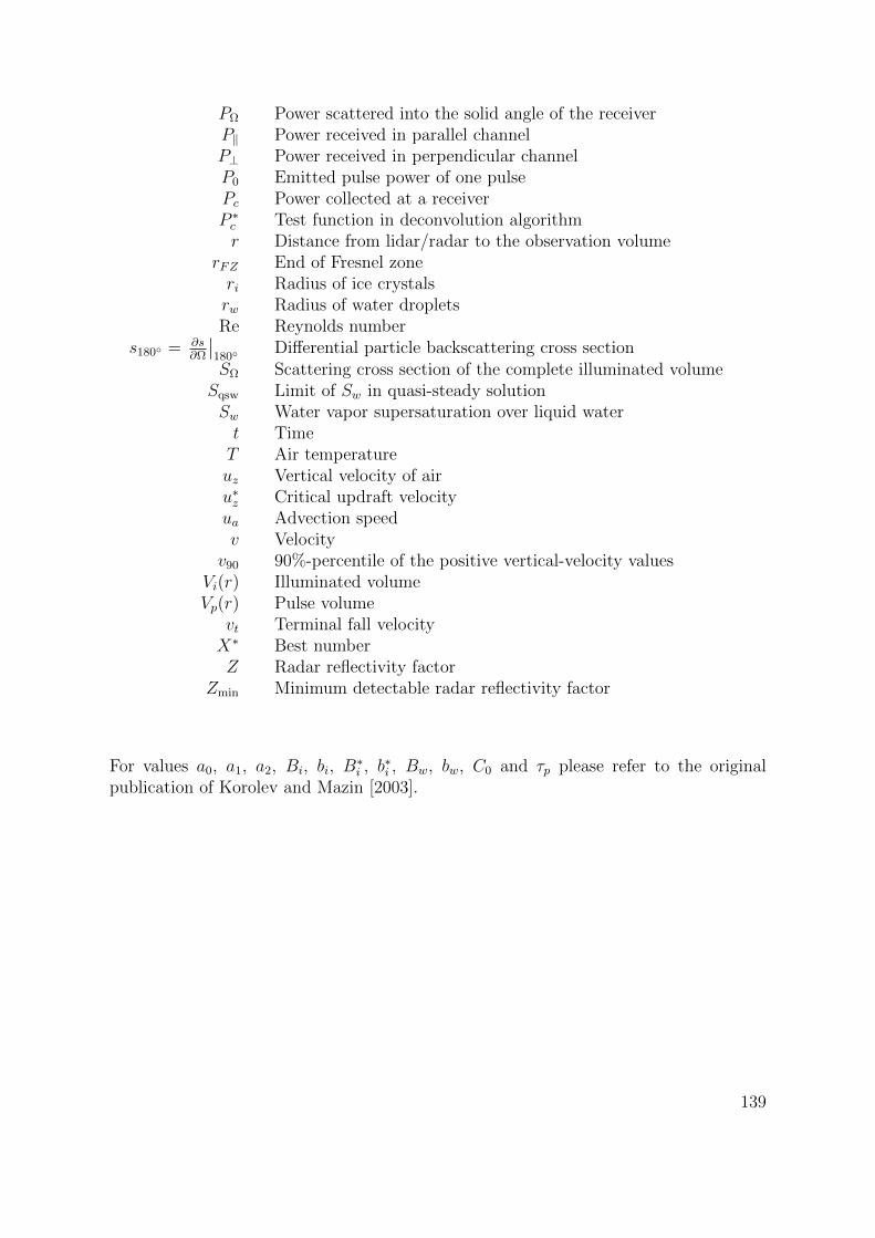
PΩ Power scattered into the solid angle of the receiverP‖ Power received in parallel channelP⊥ Power received in perpendicular channelP0 Emitted pulse power of one pulsePc Power collected at a receiverP ∗c Test function in deconvolution algorithmr Distance from lidar/radar to the observation volume
rFZ End of Fresnel zoneri Radius of ice crystalsrw Radius of water dropletsRe Reynolds number
s180 = ∂s∂Ω
∣∣180
Differential particle backscattering cross sectionSΩ Scattering cross section of the complete illuminated volume
Sqsw Limit of Sw in quasi-steady solutionSw Water vapor supersaturation over liquid watert TimeT Air temperatureuz Vertical velocity of airu∗z Critical updraft velocityua Advection speedv Velocity
v90 90%-percentile of the positive vertical-velocity valuesVi(r) Illuminated volumeVp(r) Pulse volume
vt Terminal fall velocityX∗ Best numberZ Radar reflectivity factor
Zmin Minimum detectable radar reflectivity factor
For values a0, a1, a2, Bi, bi, B∗i , b
∗i , Bw, bw, C0 and τp please refer to the original
publication of Korolev and Mazin [2003].
139

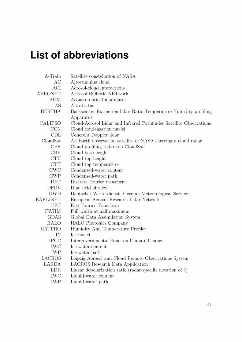
List of abbreviations
A-Train Satellite constellation of NASAAC Altocumulus cloud
ACI Aerosol-cloud interactionsAERONET AErosol RObotic NETwork
AOM Acousto-optical modulatorAS Altostratus
BERTHA Backscatter Extinction lidar–Ratio Temperature Humidity profilingApparatus
CALIPSO Cloud-Aerosol Lidar and Infrared Pathfinder Satellite ObservationsCCN Cloud condensation nucleiCDL Coherent Doppler lidar
CloudSat An Earth observation satellite of NASA carrying a cloud radarCPR Cloud profiling radar (on CloudSat)CBH Cloud base heightCTH Cloud top heightCTT Cloud top temperatureCWC Condensed-water contentCWP Condensed-water pathDFT Discrete Fourier transform
DFOV Dual field of viewDWD Deutscher Wetterdienst (German Meteorological Service)
EARLINET European Aerosol Research Lidar NetworkFFT Fast Fourier Transform
FWHM Full width at half maximumGDAS Global Data Assimilation SystemHALO HALO Photonics Company
HATPRO Humidity And Temperature ProfilerIN Ice nuclei
IPCC Intergovernmental Panel on Climate ChangeIWC Ice-water contentIWP Ice-water path
LACROS Leipzig Aerosol and Cloud Remote Observations SystemLARDA LACROS Research Data Application
LDR Linear depolarization ratio (radar-specific notation of δ)LWC Liquid-water contentLWP Liquid-water path
141
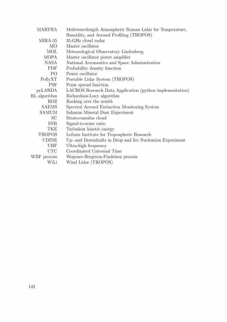
MARTHA Multiwavelength Atmospheric Raman Lidar for Temperature,Humidity, and Aerosol Profiling (TROPOS)
MIRA-35 35-GHz cloud radarMO Master oscillator
MOL Meteorological Observatory LindenbergMOPA Master oscillator power amplifierNASA National Aeronautics and Space Administration
PDF Probability density functionPO Power oscillator
PollyXT Portable Lidar System (TROPOS)PSF Point spread function
pyLARDA LACROS Research Data Application (python implementation)RL algorithm Richardson-Lucy algorithm
ROZ Rocking over the zenithSAEMS Spectral Aerosol Extinction Monitoring System
SAMUM Saharan Mineral Dust ExperimentSC Stratocumulus cloud
SNR Signal-to-noise ratioTKE Turbulent kinetic energy
TROPOS Leibniz Institute for Tropospheric ResearchUDINE Up- and Downdrafts in Drop and Ice Nucleation Experiment
UHF Ultra-high frequencyUTC Coordinated Universal Time
WBF process Wegener-Bergeron-Findeisen processWiLi Wind Lidar (TROPOS)
142