combining conventional ground-based and remotely sensed
TRANSCRIPT

Com
bining conventional ground-based and remotely sensed forest m
easurements
Mathieu D
ecuyper 2018
Combining conventional ground-based
and remotely sensed forest measurements
Mathieu Decuyper

ix
Combining conventional ground-based and remotely sensed forest measurements
Mathieu Decuyper

ii
Thesis committee Promotors Prof. Dr M. Herold Professor of Geo-information Science and Remote Sensing Wageningen University & Research Prof. Dr F.J.J.M. Bongers Personal chair at the Forest Ecology and Forest Management Group Wageningen University & Research Co-promotor Dr J.G.P.W. Clevers Associate Professor, Laboratory of Geo-information Science and Remote Sensing Wageningen University & Research Other members Prof. Dr D. Kleijn, Wageningen University & Research Prof. Dr A. Bräuning, Friedrich-Alexander Universität Erlangen-Nürnberg, Germany Dr T.A. Groen, University of Twente, Enschede Dr M. Réjou-Méchain, Institute of Research for Development, Montpellier, France This research was conducted under the auspices of the C.T. de Wit Graduate School of Production Ecology & Resource Conservation (PE&RC)

iii
Combining conventional ground-based and remotely sensed forest measurements
Mathieu Decuyper
Thesis submitted in fulfilment of the requirements for the degree of doctor
at Wageningen University by the authority of the Rector Magnificus,
Prof. Dr A.P.J. Mol, in the presence of the
Thesis Committee appointed by the Academic Board to be defended in public
on Monday 17 December 2018 at 1.30 p.m. in the Aula.

iv
Mathieu Decuyper Combining conventional ground-based and remotely sensed forest measurements, 128 pages. PhD thesis, Wageningen University, Wageningen, the Netherlands (2018) With references, with a summary in English ISBN 978-94-6343-524-6 DOI: 10.18174/462347

v
Contents
Summary............................................................................................................................... vii 1. Introduction...................................................................................................... 1 2. 50 years of groundwater extraction in the Pampa del Tamarugal basin: can Prosopis tamarugo trees survive in the hyper-arid Atacama Desert (Northern Chile)?..........................................................................................................13 3. A multi-scale approach to assess the effect of groundwater extraction on Prosopis tamarugo in the Atacama Desert..............................................................35 4. Spatio-temporal assessment of beech growth in relation to climate in Slovenia – An integrated approach using remote sensing and tree-ring data.................................................................................................................55 5. Assessing the structural differences between tropical forest types using Terrestrial Laser Scanning...................................................................................71 6. Synthesis..........................................................................................................87 References.............................................................................................................................97 Acknowledgements.............................................................................................................117 Author publications.............................................................................................................119 About the author.................................................................................................................123 PE&RC Training and Education statement........................................................................125

vi

vii
Summary
The world’s natural ecosystems are under pressure due to land conversion and climate change. Forests are a major part of these natural ecosystems and cover up to 30% of the earth’s surface. Trees are crucial for timber, store carbon, and provide other ecosystem functions. Assessing and predicting forest ecosystem responses based on global environmental changes is an important task for scientists. For many decades monitoring of forest ecosystems has been implemented using various well established (conventional) methods, but in more recent decades remote sensing techniques have made steep developments and provide opportunities in this respect. Although conventional monitoring has proven its value in many cases, monitoring forest ecosystems for decision making often requires large scale monitoring. In this sense, remote sensing (RS) offers a solution and has been successfully used for monitoring forest disturbance at regional and global scales. However, remote sensing also has made advances at plot scale, for example using near-sensing terrestrial laser scanning (TLS). Despite the potential for close collaborations between the remote sensing and forest ecology communities, there is still a disconnect (e.g. spatial / temporal resolution of data) between the two fields of expertise, which means that combining data from the two fields is difficult. To better understand for example tree physiological processes using remote sensing, further synchronisation of the two fields is vital for improving the potential for satellite data. In this thesis, I explored how to link conventional ground-based methods with remote sensing techniques, using both satellite and novel near-sensing TLS in order to investigate aspects of forest change. To do this, I looked at four representative cases with different forest types, which were selected to address different current environmental challenges with indirect (reduced tree vitality) and direct (change in forest structure) impacts. In chapter 2, we attempted to upscale ground-based conventional forest canopy measurements at plot level to remote sensing derived indices of the canopy in the Pampa del Tamarugal aquifer, in the hyper-arid Atacama desert of Chile. We assessed the foliage loss (dry branches) of the Prosopis tamarugo Phil. (a native tree) by ground-based visual assessment and digital pictures over three groundwater depletion conditions. These pictures were segmented and classified into green and brown canopy to derive the GCF (green canopy fraction). The GCF was then related to NDVIw (NDVI in winter time) from the WorldView2 satellite data, and NDVIw was used to estimate and thus upscale the GCF to all P. tamarugo trees in the aquifer. NDVIw derived from the Landsat archive allowed us to not only assess the current status of the P. tamarugo trees, but also changes over time. In this study we could

Summary
viii
successfully link ground-based conventional forest canopy measurements to remote sensing derived indices of the canopy. This allowed us, in combination with the groundwater level grids, to assess the tree vitality of the whole aquifer and determine a critical groundwater depth of 20 m for the P. tamarugos survival. Chapter 3 and 4 link ring width (RW) data at plot level to remote sensing derived plot level indices of the canopy. In both chapters the aim was to better understand the effect of environmental factors (e.g. water shortage) on the growth of trees both from the stem (wood) and canopy perspective. In Chapter 3 we used the GCF (current situation) and NDVI-based indices (historical situation) from satellite data derived from chapter 2, and assessed the correlation between NDVI-based satellite indices with ground-based tree-ring increments in two contrasting sites (low and high groundwater depletion). Time-series analysis (over a period of 26 years) and NDVI-derived parameters showed significant negative trends in the high-depletion site, indicating drought stress. Ring width of P. tamarugo trees was 48% lower in the high-depletion site. At the tree level, the GCF in the highly depleted site also indicated drought stress since a larger percentage of trees fell within lower GCF classes. In this case monitoring water shortage over time was straightforward since the stand was monospecific, and water shortage happened gradually. This was not the case in chapter 4 where we addressed the effect of climate on tree growth by combining tree-ring data of 25 locations in Slovenia with remote sensing derived EVI indices (enhanced vegetation index) from MODIS (Moderate Resolution Imaging Spectroradiometer) satellite data. We attempted to upscale the results at plot scale to national level for the tree species Fagus sylvatica L. (Beech) in the temperate forests of Slovenia. We were not able to find any relations of both RW and EVI based anomalies with climate parameters, nor was there a relation between RW and EVI based anomalies. Reasons might be: (i) time-series length (i.e. overlap between the data types), (ii) complexity of the environmental stress, such as the interplay of climatic conditions with other factors such as topography (also depending on the timing and duration of a climate event within the year), (iii) a satellite pixel might consist of other tree species less sensitive to drought, and (iv) empirical linkage between parameters – uncertainty about the direct relationship between stem and canopy derived parameters. We did find indications that both RW and EVI based anomalies were negatively affected by the extreme climate events in Slovenia, in particular the effect of the ice storm of 2014. Combining dendrochronology and remote sensing allowed us to understand the effects of drought stress on two different carbon pools (crown and stem, respectively), providing more insights on the physiological response of the species to drought. In Chapter 5 we investigated forest structure in tropical forests in Ethiopia. Here we combined conventional forest inventory measurements such as biomass, tree density, and

Summary
ix
tree species, with near-sensing TLS measurements such as PAVD (plant area vegetation density) and canopy openness. Differences between four forest types (intact forest, coffee forest, silvopasture, and plantation) for both conventional and TLS measurements were assessed. Results showed that the 3D vegetation structure (i.e. PAVD) and canopy parameters could be used to differentiate between forest types. TLS as tool for monitoring forest structure showed potential as it can capture the 3D position of the vegetation volume and open spaces at all heights. To quantify changes in different forest types, consistent monitoring of 3D structure is needed and here TLS is an add-on or an alternative to conventional forest structure monitoring. This thesis contributes to the exploration of the advantages of combining conventional ground-based data and remote sensing derived data. Combining both data types can mutually enhance the potential capabilities of each other. Remote sensing can upscale plot data to large spatial scales, while near sensing tools such as TLS can provide detailed forest structural data. Conventional ground-based data provide insight into the ecology of stands, e.g. RW or ecophysiological processes, and can help to understand remote sensing derived canopy indices. Advances in remote sensing are moving towards higher spatial, temporal, and spectral detail, but without the in-situ ecological data these advances do not reach their full potential. I, therefore, strongly advocate closer collaborations between the two research fields in the set-up of monitoring campaigns (e.g. different spatial scales). In this thesis I explored the value of combing the two fields in an empirical way. However, not all issues have been solved and more research is needed. Future research could focus on an integrated and tree-centred approach that can help to understand climate-growth interaction and the connections between stem and canopy derived indices. Future challenges also lay in improving the data operability and data processing. For remote sensing to become a conventional method, it has to become more ecologically (ecosystem) driven in an operational and cost-effective way.


1
Chapter
1
General introduction
1.1 Background The world’s forest ecosystems are under high pressure due to land conversion (Hosonuma et al., 2012) and climate change (IPCC, 2013). Forests are a major part of the world’s natural ecosystems and cover around 30% of the earth’s surface (FAO, 2017). Forests are not only needed for timber and other resources, but also provide ecosystem functions such as carbon storage and biodiversity. The approximately 4 billion hectares of forest ecosystems worldwide change constantly in both extent and vitality, making forest monitoring crucial (FAO, 2015). Between 2000 and 2015, approximately 90,000 km2 of forest has been lost per year in the tropics (Carter et al., 2018). Forests are under threat by anthropogenic pressure and conversion of forest to agriculture resulted in 72% of forest loss between 1990 and 2015 (Carter et al., 2018). After agriculture, mining, infrastructure, and urban expansion are responsible for much of the rest of forest loss (Hosonuma et al., 2012). Deforestation is almost always detrimental for biodiversity. In addition, it causes greenhouse gas emissions due to loss of an important carbon sink, which is detrimental for future climate change mitigation. Forest degradation, however, affects standing forests, where the land cover remains forest. For example, illegal logging, often occurring at smaller scales than large-scale clearances for agriculture, is responsible for altering the forest structure underneath the canopy. This has large impacts on the forest biodiversity, although not always negatively as it creates niches for different animal and plant species (Tews et al., 2004). An important component of the Paris Agreement is the REDD+ (Reducing Emissions from Deforestation and forest Degradation and the role of conservation, sustainable management of forests and enhancement of forest carbon stocks in developing countries) mechanism, which includes both deforestation and degradation. In order to successfully implement REDD+, forests need to be monitored, and, therefore forest management practices and their effects on the forest

Chapter 1
2
structure need to be understood. In addition to REDD+, other initiatives require information from forest monitoring, such as, extent and in some cases structure in order to track their goals including the United Nations Forum on Forests, the Aichi targets under the UN convention on Biodiversity, and the Sustainable Development Goals among others. Forest monitoring provides information required to conserve and protect all forests, including temperate and tropical forests, and also provides information for forest managers who are seeking to maximize timber production and other products and services (FAO, 2018). The spatial data requirements for policy makers and other decision makers, related to forest ecosystems, are often not met by conventional measurements and could be aided by remote sensing by upscaling local measurements to large scales. While large-scale clear-cut deforestation is relatively easy to identify using remote sensing (for example using satellite images), forest degradation can be more scattered and gradual, and thus is not easy to monitor. Forest can also be indirectly threatened, for example by (air) pollution or alterations in groundwater balance, which also can cause small and gradual changes. Climate change and associated changes including rising atmospheric CO2 levels, increased mean temperature and also more frequent extreme weather events, such as summer droughts, also threaten forests (Ciais et al., 2005; IPCC, 2007). It is predicted that these changes will profoundly affect forest ecosystems; but, how precisely tree growth will respond to these changes remains unclear (Xu et al., 2013). Although increasing CO2 levels enable trees to use water more efficiently (Keenan et al., 2013), their growth may be curbed by climate-induced water shortages (Bréda et al., 2006), heat stress (Bréda et al., 2006; Ciais et al., 2005), or increased respiratory demands (Adams et al., 2009; Mcdowell et al., 2008). In the last decades, forest mortality associated with drought and heat stress has been detected worldwide (Martinez-Vilalta et al., 2012; Phillips et al., 2010). Assessing and predicting ecosystem responses to global environmental changes is an important and urgent task for scientists (Pettorelli et al., 2014). In order to better protect forests and to take appropriate management decisions, knowledge of forest ecosystem functions and monitoring of forests and their functions is crucial. Since many decades, monitoring of forest ecosystems has been done by various well established ‘conventional’ methods, but in more recent decades, remote sensing techniques have made steep developments. This thesis will explore the integration of both conventional and (novel) remote sensing techniques in assessing the anthropogenic and natural impacts on forests.
1.2 The use of conventional ground-based measurements to assess forest vitality and forest structure In this thesis I define conventional ground-based forest measurements as forest parameters that have been used for at least a decade, and that have empirically proven their operational value in the field of forest ecology. The array of ground-based measurements to assess forest
General introduction
3
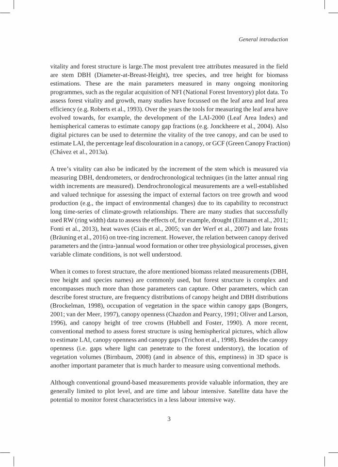
vitality and forest structure is large.The most prevalent tree attributes measured in the field are stem DBH (Diameter-at-Breast-Height), tree species, and tree height for biomass estimations. These are the main parameters measured in many ongoing monitoring programmes, such as the regular acquisition of NFI (National Forest Inventory) plot data. To assess forest vitality and growth, many studies have focussed on the leaf area and leaf area efficiency (e.g. Roberts et al., 1993). Over the years the tools for measuring the leaf area have evolved towards, for example, the development of the LAI-2000 (Leaf Area Index) and hemispherical cameras to estimate canopy gap fractions (e.g. Jonckheere et al., 2004). Also digital pictures can be used to determine the vitality of the tree canopy, and can be used to estimate LAI, the percentage leaf discolouration in a canopy, or GCF (Green Canopy Fraction) (Chávez et al., 2013a). A tree’s vitality can also be indicated by the increment of the stem which is measured via measuring DBH, dendrometers, or dendrochronological techniques (in the latter annual ring width increments are measured). Dendrochronological measurements are a well-established and valued technique for assessing the impact of external factors on tree growth and wood production (e.g., the impact of environmental changes) due to its capability to reconstruct long time-series of climate-growth relationships. There are many studies that successfully used RW (ring width) data to assess the effects of, for example, drought (Eilmann et al., 2011; Fonti et al., 2013), heat waves (Ciais et al., 2005; van der Werf et al., 2007) and late frosts (Bräuning et al., 2016) on tree-ring increment. However, the relation between canopy derived parameters and the (intra-)annual wood formation or other tree physiological processes, given variable climate conditions, is not well understood. When it comes to forest structure, the afore mentioned biomass related measurements (DBH, tree height and species names) are commonly used, but forest structure is complex and encompasses much more than those parameters can capture. Other parameters, which can describe forest structure, are frequency distributions of canopy height and DBH distributions (Brockelman, 1998), occupation of vegetation in the space within canopy gaps (Bongers, 2001; van der Meer, 1997), canopy openness (Chazdon and Pearcy, 1991; Oliver and Larson, 1996), and canopy height of tree crowns (Hubbell and Foster, 1990). A more recent, conventional method to assess forest structure is using hemispherical pictures, which allow to estimate LAI, canopy openness and canopy gaps (Trichon et al., 1998). Besides the canopy openness (i.e. gaps where light can penetrate to the forest understory), the location of vegetation volumes (Birnbaum, 2008) (and in absence of this, emptiness) in 3D space is another important parameter that is much harder to measure using conventional methods. Although conventional ground-based measurements provide valuable information, they are generally limited to plot level, and are time and labour intensive. Satellite data have the potential to monitor forest characteristics in a less labour intensive way.

Chapter 1
4
1.3 The use of remote sensing to assess forest vitality and forest structure In this thesis I consider remote sensing tools as space-based sensors, for example satellites and also remote sensing systems on the International Space Station, which are hereafter referred to as satellites, or more recent tools that operate nearby (i.e. TLS – Terrestrial Laser Scanner), or a few 100 m away (i.e. sensors mounted on airplanes or drones). In the last decades remote sensing techniques have developed fast, ranging from the improvement of satellite data resolutions (both temporal, spatial and spectral) in a new generation of spaceborne systems, to the development of the TLS technique. Satellite data not only enable forest monitoring over large areas, but also allow monitoring in otherwise inaccessible locations, thus providing advantages over conventional approaches. Satellite derived data have been used successfully to capture effects of changes in environmental conditions on tree growth in different ecoregions: for example, effects of drought on gross primary production in temperate forests (Vicca et al., 2016) and evidence of the trees’ response to drought in tropical forests (Asner and Alencar, 2010). The most commonly known remote sensing index is the NDVI (Normalized Difference Vegetation Index), which has been used a lot to evaluate forest vitality and productivity (Arrigo et al., 2010). Besides these studies, few studies are published on the effect of drought or other climate parameters on tree vitality. Direct changes due to fires, wind throws or clear cutting can be captured by satellite data, but when it comes to more complex effects of climate, it depends on the intensity and extent of disturbance, and the availability of satellite data whether detection occurs (Deshayes et al., 2006). Remote sensing has also been used to capture forest structure, although mainly in tropical forests. Satellite data have been successfully used for monitoring forest disturbance from regional to global scale (DeVries et al., 2015; Hansen et al., 2013). Clear-cut forests and large scale selective logging can be relatively easily monitored due to the almost complete loss of the canopy cover, which is easily identifiable in satellite data. However, smaller scale changes such as forest degradation are much more challenging to detect, and the ability to identify these changes depends on the spatial resolution of the satellite sensor. To estimate forest parameters such as biomass, the use of SAR (Synthetic Aperture Radar) has been successfully applied, but tends to saturate in areas with high tree density (Joshi et al., 2015). LiDAR (Light Detection And Ranging or Laser Imaging Detection And Ranging) has been used in large-scale mapping of biomass (Baccini et al., 2012; Saatchi et al., 2011); however, data are uncertain (Mitchard et al., 2014). To date, no airborne or satellite sensor has been operationally applied to monitor forest degradation, largely due to the specific nature of

General introduction
5
degradation (small scale) and the timeframe over which it occurs (Mitchell et al., 2017). No airborne or satellite sensor is able to capture forest structural estimates under the forest canopy. Recently, the TLS has shown promising advances to estimate biomass in the tropics (Gonzalez de Tanago et al., 2018), but data processing remains quite time-consuming. Very few remote sensing studies (e.g. Palace et al., 2016) looked at a wider array of forest structural characteristics, especially in the tropics.
1.4 Combining conventional ground-based measurements and remote sensing In spite of the capabilities of conventional methods (section 1.2) and the advances in remote sensing (section 1.3), there are very few studies combining both techniques. In relation to measuring the effects of drought on tree growth, Bunn et al. (2013) and Bhuyan et al. (2017) found a relation between the NDVI and RW chronologies in forests in the Northern hemisphere, but they did not focus on year-to-year climate variations. Other studies mainly used RW data as a proxy of productivity in mixed landscapes, but did not directly relate RW data to remote sensing derived indices (Coulthard et al., 2011; Southworth et al., 2013b). Thus, the understanding of how climate extremes such as drought affect trees is still limited (Norman et al., 2016). Changes in vegetation functioning, especially when vegetation does not show severe changes such as browning or defoliation, are difficult to capture using satellite-derived indicators (Vicca et al., 2016). Satellites primarily can measure the above-ground foliage and, although the leaves are crucial in the photosynthesis process, it is still a proxy for wood production. Thus, satellite data alone cannot provide enough information to understand trees’ responses to, e.g., climate changes. Plot level data also are often not sufficient to cover the spatial scales needed for policy makers and here remote sensing data could play an important role in upscaling the information obtained at plot level. Therefore, integration of space-based remote sensing data with ground-based data is essential to understand the trees’ response to environmental effects. Integration of methods is also important when dealing with forest structure, especially when assessing forest degradation with subtle changes underneath the canopy. Changes below the canopy can strongly alter the forest structure and have large impacts on biodiversity too (Barlow et al., 2016; Pettorelli et al., 2014). Due to anthropogenic pressure not only forest structure, but directly and indirectly fauna is affected, sometimes to an extreme degree with no large animals remaining under the intact forest canopy – i.e. the “empty forest” theory of Redford (1992). Accurate characterization and measurement of the intensity of forest management and use and thus the drivers of forest degradation is required in order to take management actions to prevent further degradation and to plan restoration actions (Ghazoul et al., 2015; Ghazoul and Chazdon, 2017). However, few studies deal with these subtle
Chapter 1
6
changes in forest structure from a remote sensing perspective, particularly in the tropics. Palace et al. (2016, 2015) captured tree density, basal area and tree density in tropical forests, and Couteron et al. (2012) used a physical approach to derive forest structure using radiative transfer models, which enabled the linkage between remote sensing and in-situ measurements. Recently developed novel sensing tools such as TLS have provided opportunities to measure forest structure and have the potential of reducing the uncertainty of conventional in-situ measurements. However, conventional measurements such as tree species names and some plant functional traits (e.g. leaf thickness) cannot be captured by TLS. For this reason the integration with conventional ground-based data is needed. From the satellite and airborne based sensors, SAR and LiDAR sensors show the most promise for quantifying AGB (above ground biomass), but still need field data to model AGB (Mitchell et al., 2017). However, no satellite or airborne sensor can capture subtle forest structural parameters underneath the canopy, so there is a need for ground-based sensor data or conventional field measures.
1.5 Objectives Despite the potential for close collaborations between the remote sensing and forest ecologist communities, there is still a disconnect between the two fields of expertise, which means that combining data from the two fields is difficult. This is due to the differences in the data derived from remote sensing and from conventional monitoring, such as the spatial / temporal resolution, definitions (of forest or biomass for example) and differences in terms of what is measured. In an operational sense, existing ground data (for example NFI plot data) might be combined with remote sensing data. To do this, the location of a plot defined by the ecologist needs to be known so that it can be linked to a specific pixel(s) in a remote sensing image. Often biomass plots are not large enough to cover one or multiple remote sensing pixels or in some case the exact plot location is even not known, meaning that it is very difficult to combine different datasets. Despite the above mentioned issues, the fast advances in technology (especially remote sensing techniques) provide opportunities to overcome problems such as differences in scale (finer resolution data). Forests face many threats from climate change and degradation. Some of these threats, such as the scale of insect outbreaks (increased outbreaks due to warmer conditions) are more difficult to map based on in-situ data alone and can benefit from the increased availability of satellite data. To better understand climate-growth relations related to these threats (e.g. tree physiological processes) or monitor forest structural parameters (e.g. to capture the effect of management practices) by remote sensing monitoring, further synchronising the two fields (coordination of data collection, or sharing existing data with extensive meta-information) is vital to improve the potential for satellite, airborne and ground-based remote sensing.
General introduction
7
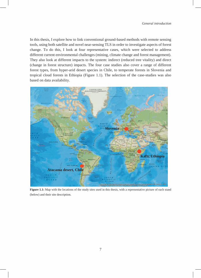
In this thesis, I explore how to link conventional ground-based methods with remote sensing tools, using both satellite and novel near-sensing TLS in order to investigate aspects of forest change. To do this, I look at four representative cases, which were selected to address different current environmental challenges (mining, climate change and forest management). They also look at different impacts to the system: indirect (reduced tree vitality) and direct (change in forest structure) impacts. The four case studies also cover a range of different forest types, from hyper-arid desert species in Chile, to temperate forests in Slovenia and tropical cloud forests in Ethiopia (Figure 1.1). The selection of the case-studies was also based on data availability.
Figure 1.1: Map with the locations of the study sites used in this thesis, with a representative picture of each stand (below) and their site description.
Atacama desert, Chile
Slovenia
Kafa, Ethiopia

Chapter 1
8
Beech (Fagus sylvatica L.) forest in Slovenia. One of the dominant tree species in the country with high economic value. Beech forests are generally characterised by their low understory growth. Recently (last 6 years) many climate extremes have occurred which might affect the tree growth.
Prosopis tamarugo Phil. trees in the hyper-arid Atacama desert, Chile. The Pampa del Tamarugal aquifer is a salt plane in which mainly P. tamarugo grows. Precipitation is virtually non-existent, and is highly dependent on groundwater flows from eastern sub-basins (Rojas and Dassargues, 2007). In many places in the aquifer, ground water extraction poses a threat to the survival of this native tree.

General introduction
9
Within the framework of this PhD thesis the following research questions have been formulated: 1. How can ground-based conventional forest canopy measurements be linked to remote sensing derived indices of the canopy? This research question is answered by assessing a specific forest ecosystem with hyper-arid conditions, and with a specific stress (water shortage due to groundwater depletion). 2. How can individual tree-based dendrochronological measurements be linked to remote sensing derived plot level indices? Very few studies have attempted to combine RW with remote sensing derived indices. In this thesis I study this in two different forest types (P. tamarugo in the hyper-arid Atacama desert in Chile; and beech forest in temperate regions in Slovenia.) 3. What is the added value of ground-based TLS in addition to established ground-based forest structural measurements? This question is more technology driven and aims to explore new opportunities of near-sensing TLS to assess the effect of management practices in montane cloud forests in Ethiopia.
Tropical montane cloud forests in the Kafa Biosphere Reserve, Ethiopia. This biosphere is a biodiversity hotspot and is considered the origin of the Coffea arabica. Forests range from intact core forests, to coffee forests, silvopastures and plantations. This forest is under threat due to degradation.

Chapter 1
10
1.6 Thesis structure The remainder of this chapter describes the framework of the thesis (Figure 1.2). This thesis consists of six chapters, including this introduction. Chapter 2 addresses the first research question, where we attempt to upscale ground-based conventional forest canopy measurements at plot level to remote sensing derived indices of the canopy in the Pampa del Tamarugal aquifer. Chapters 3 and 4 mainly focus on research question 2, aiming to link RW data at plot level to remote sensing derived plot level indices, in order to better understand the effect of environmental factors (e.g. water shortage) on the growth of trees both from the stem (wood) and canopy perspective. In chapter 5 we assess forest structure in different forest types by complementing conventional ground-based data with near-sensing TLS derived data. The case studies in chapters 2 and 3 deal with a single species (P. tamarugo), whereas chapters 4 and 5 are more complex with mixed species case studies. Chapter 2 presents the relation between visually assessed Green Canopy Fraction (GCF) combined with GCF derived from ground-based photographs with satellite-based GCF to assess the effect of groundwater depletion on Prosopis tamarugo Phil. in the Atacama desert in Chile. Furthermore, we performed a spatial-temporal assessment of the whole aquifer using NDVI-derived indices from satellite data (upscaling). In Chapter 3 we use the GCF and NDVI-based indices from satellite data derived from chapter 2 and assess the correlation between NDVI-based satellite indices with ground-based tree-ring increments over a 24-year time span. This was done in two contrasting sites (low and high groundwater depletion). The GCF is used to provide more information on the current differences between the two sites. Chapter 4 addresses the effect of climate on tree growth by combining tree-ring data of 25 locations in Slovenia with remote sensing derived EVI indices (Enhanced Vegetation Index) from MODIS (Moderate Resolution Imaging Spectroradiometer) satellite data. We attempt to upscale the results at plot scale to national level for the tree species Fagus sylvatica L. (Beech). In chapter 5 we look at forest structure in a tropical montane cloud forest in Ethiopia. Here, we use a combination of established ground measurements such as biomass, and assess the added value of near-sensing TLS derived forest structural parameters such as PAVD (Plant Area Volume Density) in plots with different management practices. This thesis is concluded in chapter 6, where I discuss the main findings of the case studies and the potential of the integration of conventional ground-based measurements with those derived from remote sensing. I assess the lessons learned and give recommendations for

General introduction
11
future research by discussing the integration with newly available techniques such as near-sensing with the aid of drones and high resolution satellite images.
Figure 1.2: Conceptual framework linking the ground-based conventional measurements (green) with the remote sensing derived measurements (blue), and environmental factors (beige).

12

13
Chapter
2 1 50 years of groundwater extraction in the Pampa
del Tamarugal basin: can Prosopis tamarugo trees survive in the hyper-arid Atacama Desert
(Northern Chile)?
R.O. Chávez, J.G.P.W. Clevers, M. Decuyper, S. De Bruin, M. Herold
This chapter is based on: Journal of Arid Environments, 124 (2016), pp. 292-303
DOI: 10.1016/j.jaridenv.2015.09.007
Supplementary material mentioned in the text can be found in the online publication Groundwater-dependent ecosystems are threatened worldwide by unsustainable groundwater (GW) extraction. This is the case of the Prosopis tamarugo Phil forest in the hyper-arid Atacama Desert (Northern Chile), one of the most extreme ecosystems on Earth. Despite concerns about the conservation of this ecosystem, little research has been done to quantify the effects of the increasing GW depth (GWD) on the P. tamarugo population. Here we provide a spatio-temporal assessment of the water condition of P. tamarugo trees and propose GWD thresholds for their conservation. We studied spatio-temporal changes of GWD and the water status of the forest using Landsat images and hydrogeological records (1988–2013). This was complemented with a digital inventory and estimation of the green canopy fraction (GCF) of all trees using fine resolution satellite images. Since P. tamarugos are solar trackers, their canopy spectral reflectance changes on a diurnal and seasonal basis. Thus, novel remote sensing drought stress indicators were defined: the mean NDVI in winter (NDVIw) accounting for foliage loss and the NDVI difference between mean winter and summer (ΔNDVIw-s) accounting for canopy water loss. NDVIw and ΔNDVIw-s of the P. tamarugo forest declined on average 19% and 51%, respectively, while GW depleted on average 3 m over the period 1988–2013. About 730,000 trees were identified in the study area, from which

Chapter 2
14
5.2% showed a GCF < 0.25 associated with severe drought stress. A GWD > 12 m increasingly limited the paraheliotropic leaf movement, leading to dehydration and foliage loss. P. tamarugo at 12–16 m GWD suffered moderate drought stress while GWD of 16–20 m implied severe drought stress. We suggest 20 m GWD as a critical threshold for the survival of P. tamarugo trees.
Keywords
Arid ecosystems; water stress; groundwater extraction; time series; remote sensing; normalized difference vegetation index; water management
2.1 Introduction Water is a limiting resource for wildlife and human activities in arid and semi-arid areas. As national economies develop, the pressure for using the scarce water sources of desert basins to provide water to urban centers and industry increases, becoming a threat for desert ecosystems worldwide (Ezcurra, 2006; Pringle, 2001). The main water source in deserts is the groundwater (GW) and several authors have highlighted the importance of assessing the negative impacts of GW extraction on natural vegetation (Elmore et al., 2006, 2003; Naumburg et al., 2005; Patten et al., 2008). Desert vegetation provides important ecosystem services such as the regulation of the hydrological cycle, the conservation of endemic and rare species, and the provision of an oasis for local settlements, grazing and small scale agriculture (Ezcurra, 2006). The expected decrease in available fresh surface water due to global warming together with the future increase of water consumption at global scale, make GW overexploitation likely to occur (Wang et al., 2014). As a result, the main challenge for water managers today is to promote a sustainable exploitation of GW aquifers compatible with the conservation of desert ecosystems (Elmore et al., 2003). Chilean environmental institutions are already facing such a challenge in the Pampa del Tamarugal aquifer, where one of the most extreme desert ecosystems still remains in the heart of the Atacama Desert (Northern Chile).
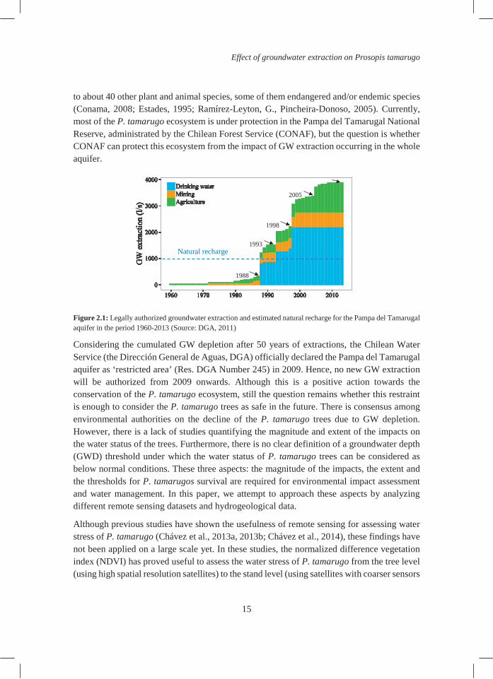
The Pampa del Tamarugal aquifer is the only source of drinking water for a large area in the Atacama Desert and for more than 50 years GW has been extracted to supply water to urban areas (including important cities like Iquique), the mining industry and agriculture (Figure 2.1). From 1988 onwards the authorized GW extractions have exceeded the natural recharge of the aquifer (Figure 2.1) inducing a depletion of the GW table in the whole aquifer (Rojas et al., 2010; Rojas and Dassargues, 2007). This unbalance in the water budget is threatening the P. tamarugo ecosystem, which is completely dependent on GW and limited to the areas with shallow GW. The main species of this ecosystem is the P. tamarugo tree: an endemic tree species of the Atacama Desert. The ‘Pampa del Tamarugal’ formation provides habitat
Effect of groundwater extraction on Prosopis tamarugo
15
to about 40 other plant and animal species, some of them endangered and/or endemic species (Conama, 2008; Estades, 1995; Ramírez-Leyton, G., Pincheira-Donoso, 2005). Currently, most of the P. tamarugo ecosystem is under protection in the Pampa del Tamarugal National Reserve, administrated by the Chilean Forest Service (CONAF), but the question is whether CONAF can protect this ecosystem from the impact of GW extraction occurring in the whole aquifer.
Figure 2.1: Legally authorized groundwater extraction and estimated natural recharge for the Pampa del Tamarugal aquifer in the period 1960-2013 (Source: DGA, 2011)
Considering the cumulated GW depletion after 50 years of extractions, the Chilean Water Service (the Dirección General de Aguas, DGA) officially declared the Pampa del Tamarugal aquifer as ‘restricted area’ (Res. DGA Number 245) in 2009. Hence, no new GW extraction will be authorized from 2009 onwards. Although this is a positive action towards the conservation of the P. tamarugo ecosystem, still the question remains whether this restraint is enough to consider the P. tamarugo trees as safe in the future. There is consensus among environmental authorities on the decline of the P. tamarugo trees due to GW depletion. However, there is a lack of studies quantifying the magnitude and extent of the impacts on the water status of the trees. Furthermore, there is no clear definition of a groundwater depth (GWD) threshold under which the water status of P. tamarugo trees can be considered as below normal conditions. These three aspects: the magnitude of the impacts, the extent and the thresholds for P. tamarugos survival are required for environmental impact assessment and water management. In this paper, we attempt to approach these aspects by analyzing different remote sensing datasets and hydrogeological data.
Although previous studies have shown the usefulness of remote sensing for assessing water stress of P. tamarugo (Chávez et al., 2013a, 2013b; Chávez et al., 2014), these findings have not been applied on a large scale yet. In these studies, the normalized difference vegetation index (NDVI) has proved useful to assess the water stress of P. tamarugo from the tree level (using high spatial resolution satellites) to the stand level (using satellites with coarser sensors
Natural recharge
1988
1993
1998
2005

Chapter 2
16
such as Landsat or MODIS). These authors highlighted that P. tamarugo trees are heliotropic plants or ‘solar trackers’, an important botanical fact to consider for remote sensing based assessments. P. tamarugos sense the increasing solar irradiation during the day and adjust the orientation of their leaves (leaf pulvinar movements) to avoid facing the sun rays at the hottest time of the day, causing a diurnal variation in the NDVI signal (Chávez et al., 2013a, 2013b). Similarly, this mechanism gets more active in summer than in winter, causing a seasonal variation in the NDVI signal with low values in summer and high values in winter (Chávez et al., 2014).
Chávez et al. (2014) showed that the mean NDVI in winter (NDVIw) was negatively correlated to cumulative GW depletion, in other words NDVIw decreases as GWD increases. In the same study the authors proposed a new water stress indicator: the NDVI difference between winter and summer (ΔNDVIw-s), which was related to the capacity of P. tamarugo to perform leaf pulvinar movements. Due to its nature, ΔNDVIw-s was considered an early indicator of water stress, since the limitation of the leaf movements occurred under stress before P. tamarugo started shutting down green foliage (Chávez et al. 2013a; Chávez et al. 2013b). In this paper, we hypothesize that both indicators (NDVIw and ΔNDVIw-s) are spatially and temporally correlated to GWD, making a quantitative assessment of the impacts of GW extractions in the Pampa del Tamarugal aquifer possible. Furthermore, we aim to provide useful information for operational P. tamarugos conservation practices and GW management by combining the high temporal resolution of Landsat with HSR satellite images.
Besides the local national application, this contribution aims to provide a remote sensing based approach to detect and quantify drought stress on paraheliotropic (‘solar tracking’) vegetation, a common adaptation to semi-arid and arid environments.
2.2 Material and methods
2.2.1 Species description P. tamarugos are thorny desert trees highly specialized to survive the aridness of the hyper-arid Atacama Desert, a place considered among the more extreme environments for life (McKay et al., 2003; Navarro-gonza et al., 2003). This endemic species of the Atacama Desert belongs to the Leguminoseae family and exhibits a large range of phenotypes. In adverse conditions, P. tamarugos express a shrub-like phenotype, about two m high and 2-3 m crown size, while P. tamarugos express a tree-like phenotype under favourable conditions, reaching up to 25 m high and 20-30 m crown size (Altamirano, 2006; Chávez et al., 2013a; Riedemann et al., 2006).

Effect of groundwater extraction on Prosopis tamarugo
17
Several adaptations to survive the harsh conditions of the Atacama Desert have been described for P. tamarugo. They are phreatophytic species (Mooney et al., 1980) with a dual root system: a deep taping root and a dense superficial root mat (Sudzuki, 1985a). It has been suggested that P. tamarugos’ root system moves water from the GW to the root mat layer during the night to ensure water supply during the growing season when the water demand at the capillary fringe increases (Mooney et al. 1980). Furthermore, like other Legiminoseae plants P. tamarugo trees are solar trackers (Chávez et al. 2013a; Chávez et al. 2013b). They adjust the angle of the leaves as solar irradiation increases to avoid facing direct sun rays at the hottest time of the day (paraheliotropism) and this way enhance the photosynthetic process and avoid photoinhibition. Paraheliotropic leaf movements have been reported for many other desert plants and some major crops (Ehleringer and Forseth 1980; Pastenes et al. 2005; Pastenes et al. 2004). Another remarkable adaptation is its osmotic regulation capacity allowing rapid stomata closure as temperature and vapour pressure deficit increase during the day (Acevedo et al., 1985; Ortiz et al., 2010). In summary, P. tamarugos optimize the water budget by enhancing the GW intake and by reducing evapotranspiration due to excessive solar irradiation.
2.2.2 Study area The study area comprises all P. tamarugo plantations of the ‘Lote3’ of Pampa del Tamarugal National Reserve and some plantation stands and natural vegetation located in private areas surrounding the Reserve (Figure 2.2). The study area covers the two sectors where most of the remaining P. tamarugo population is concentrated: the Salar de Pintados and the Salar de Bellavista. Both sectors are located in the south-west part of the Pampa del Tamarugal aquifer where the GW table is relatively shallow (5-15 m). Since GW levels are close to the surface, these sectors show a high evaporation causing salt accumulation in the upper layers of the soil (Houston, 2006a). This has led to the formation of salt-flats, locally known as ‘salares’, with Salar de Pintados and Salar de Bellavista as the largest ones in the Pampa del Tamarugal Aquifer.
The Pampa del Tamarugal aquifer is situated in the dry plains located between the Andes mountain range and the Pacific Ocean, covering an area of about 5,000 km2 (Rojas and Dassargues, 2007). It is 130-160 km long, 13-60 km wide and located 45 km away from the coast line at an altitude of 1,000 m (JICA-DGA-PCI, 1995; Rojas and Dassargues, 2007). Since precipitation is practically inexistent, the recharge comes laterally from the eastern sub-basins through infiltration and GW flow (Houston, 2002; Rojas and Dassargues, 2007). Several authors have estimated the recharge of the aquifer (DICTUC, 2008, 1988; JICA-DGA-PCI, 1995; Rojas and Dassargues, 2007), showing a general agreement on a value of about 1,000 l/s. However, artificial discharge (pumping) has dramatically increased since the

Chapter 2
18
1980’s causing a sustained negative water balance and an overall lowering of the GW table (CIDERH, 2013; Rojas and Dassargues, 2007).
Figure 2.2: Landsat mosaic showing the study area in the Atacama Desert (Northern Chile). Monitoring wells from the DGA network (updated to 2013) and extraction wells from DGA (2011).

Effect of groundwater extraction on Prosopis tamarugo
19
The natural P. tamarugo trees were almost extinct in the 19th century due to overexploitation for wood supply and fuel for the saltpetre industry (Zelada, 1986). Although there were attempts to reforest Pampa del Tamarugal as early as 1936, it was not until the 1970’s when an enormous reforestation effort was carried out by the Chilean government and about 13,000 hectares were planted. Trees were planted in 40 cm deep holes in a regular 10x10 m grid by removing the salt crust. Plants were put in the shadowed south base of the holes and watered during the first year of establishment till the root system was tapping the GW (Habit et al., 1981; Mooney et al., 1980). During the reforestation of the Pampa del Tamarugal also some other Prosopis species were planted, sometimes mixed with P. tamarugo. Nevertheless, only pure P. tamarugo stands were considered in this study (see the green areas in Figure 2.2).
2.2.3 Hydrogeological data We collected available data of extraction wells, monitoring wells and historical GWD maps of the Pampa del Tamarugal aquifer, complemented with precipitation records. Although precipitation hardly occurred in the study area, the few rainfall events can have an impact on the NDVI signal of the P. tamarugo forest (Chávez et al. 2014). The sources of information used in this study are:
2.2.3.1 Extraction well data (DGA 2011).
We considered the 740 extraction wells used by DGA to calculate artificial discharge from the Pampa del Tamarugal aquifer (Figure 2.2). We obtained from each well the location, the authorized GW extraction (l/s) and the year in which the extraction request was issued. We assigned this year as the starting year of extraction, since the authorization year was absent for many wells.
2.2.3.2 Monitoring wells from the DGA network (1989-2013).
We used 26 wells located in the center-south part of the aquifer with GWD records updated till December 31st, 2013 (Figure 2.2). These wells are part of the current operational DGA network. Only 13 wells had records for the period 1989-2013 and the other 13 for the period 1998-2013. The records obtained this way were used to calculate mean annual GWD values for each well considering only years with at least three measurements (see details in Appendix A, Table A1).
2.2.3.3 GWD grid maps (1988-2013).
Sources for these maps were the study of JICA-DGA-PCI (1995) for the years 1988 and 1993 and GWD interpolations made in this study using the 27 DGA monitoring wells for the period 1998-2013. For the GWD interpolations 1998-2013 we used spatial interpolation by ordinary point kriging, as implemented in the gstat package (Pebesma, 2004) of the R software (R
Chapter 2
20
Core team, 2013). Assuming temporal stationarity of the spatial correlation structure, a single experimental variogram was computed by pooling point pairs from different years. Spatio-temporal interpolation was not attempted because of lack of data for fitting a spatio-temporal variogram. An exponential variogram model was fitted (nugget = 15, psill = 280, and range = 7,000). GWD data for the period 1998-2013 were interpolated by ordinary point kriging to a square grid with 90 m spacing. We performed a leave-one-out cross-validation to check the kriging assumptions; Z-scores of the residuals were normally distributed with mean -0.01 and standard deviation of 1.28. The deviation from 1 of the standard deviation was caused by a few large residuals located outside the forested area (see Appendix A, Figure A2), corresponding to wells close to the pumping areas.
2.2.3.4 Precipitation records (1992-2013).
These were obtained from the DGA meteorological station Huara en Fuerte Baquedano, located about 30 km north from the study area (20°07'51''S, 69°44'59''W) and at similar altitude (1,100 m).
2.2.4 Landsat NDVI derived metrics We used all available Landsat 5 TM and Landsat 7 ETM data of the study area covering the period 1988-2013. A total of 667 cloud free L1T images of 30 m pixel resolution corresponding to path 1 and row 34 were downloaded and pre-processed using the Landsat Ecosystem Disturbance Adaptive Processing System (LEDAPS) to obtain surface reflectance values for all spectral bands (Masek et al., 2006). Subsequently, we used the red and near-infrared (NIR) surface reflectance values to compute the NDVI for each scene as follows: NDVI = (NIR-Red)/(NIR+Red). Using as a base the P. tamarugo plantation map of CONAF (1997) and the 3-month average Landsat NDVI of the 1988 winter, we created a forest mask with all pixels inside the P. tamarugo stands and NDVI values higher than 0.13. Then, a Landsat NDVI time series was calculated using the median value of the pixels for each scene inside the forest mask. Using this time series we calculated NDVI derived metrics for each year as follows:
(1) NDVIw = average of all NDVI scenes from the months May, June and July (winter); (2) NDVIs = average of all NDVI scenes from the months November, December and
January (summer); (3) ΔNDVIw-s = Landsat NDVIw – Landsat NDVIs.
As stated before, we considered a minimum of three scenes for the summer and winter period to obtain a representative value of the respective season. Otherwise a gap in the time series occurred. For mapping NDVI derived metrics of specific years (1988, 1993, 1998, 2005, and 2013), no ETM SLC-off scenes (containing no-data stripes due to the failure of the Scan Line

Effect of groundwater extraction on Prosopis tamarugo
21
Corrector in 2003) were used. Only 2013 was mapped using ETM SLC-off data since the TM sensor was discontinued in November 2011.
2.2.5 Digital inventory using high spatial resolution imagery Following the recommendations of Chávez et al. (2013), we performed tree identification in summer (to avoid shadows) and NDVI calculation in winter (the annual NDVI peak occurred in winter for paraheliotropic P. tamarugo trees). For this reason, a panchromatic Quickbird2 image with 0.6 m pixel resolution, acquired in November 2006, was used to automatically delineate single P. tamarugo trees in the study area. We used the procedure developed by Chávez and Clevers (2012), allowing discrimination of single trees even when the tree crowns were overlapping. This object-based algorithm provided object polygons with the crown area of each tree as output. Using these polygons, we extracted for each tree the digital values of the red and NIR bands of a WorldView2 multispectral image with 2 m pixel resolution, acquired in July 2011. The digital values of both bands were transformed into top-of-canopy reflectance following Updike and Comp (2010) to finally calculate the NDVIw for each P. tamarugo tree in 2011. Although differences in canopy size may exist between 2006 and 2011, we believe that they can be neglected since the crown growing rate of adult trees was low, which was confirmed by visual comparison of the canopy size in the panchromatic images of 2006 and 2011. Thus, differences in crown size between 2006 and 2011 were most likely smaller than the pixel resolution of the multispectral image.
During a field campaign carried out in January 2012, 50 P. tamarugo trees were surveyed. We used the procedure proposed by Chávez et al. (2013a) to calculate the green canopy fraction (GCF) of each tree using digital pictures and an object-based image segmentation of the green and brown canopy elements. We regressed the GCF and NDVI values for single trees to obtain an empirical equation, which was used to estimate GCF for all the trees identified in the digital inventory. This way, we obtained the total number of P. tamarugo trees, the total and individual crown area and an estimation of the GCF at the tree level in 2011.
2.2.6 Data analysis
2.2.6.1 Temporal patterns
We analysed the relationship between the annual average time series of NDVI derived metrics (NDVIw and ΔNDVIw-s) and GWD of the P. tamarugo areas by inspecting the trends and by calculating simple correlation coefficients (R). Annual average values were calculated by averaging all the cells (pixels) from the satellite images and GWD interpolation grids inside the forest mask (spatial mean).

Chapter 2
22
2.2.6.2 Spatial patterns
We made maps for the years 1988, 1993, 1998, 2005 and 2013 showing the location of the pumping wells, the GWD iso-curves of 5, 10, 15 and 20 m and the NDVI derived metrics. In order to provide an up-to-date assessment of the condition of the P. tamarugos after 50 years of GW extraction, we analysed the distribution of the P. tamarugo population in the GWD range of the forested area in 2011 by using histograms of the number of trees as well as the proportion of trees sorted in four classes of GCF (0-0.25, 0.25-0.50, 0.50-0.75 and > 0.75) at different GWD. In the same way we used histograms with the proportion of Landsat pixels sorted in four categories of NDVIw and ΔNDVIw-s at different GWD.
2.3 Results
2.3.1 Groundwater depth and Landsat NDVI derived metrics in the period 1988-2013 The authorized GW extraction in the Pampa del Tamarugal aquifer increased from about 400 l/s in 1988 to about 2,200 l/s in 1998 (Figure 2.1), causing an average GW depletion of about 2 m in the areas covered by P. tamarugo (Figure 2.3). By 2009, the year the aquifer was declared ‘restricted area’, the authorized GW extractions had reached about 4,000 l/s. This amount constitutes the current (2013) legal water rights in the Pampa del Tamarugal aquifer, which is four times the natural recharge of the system (estimated at about 1,000 l/s) (JICA-DGA-PCI, 1995; Rojas and Dassargues, 2007). Since 1998 GWD has increased linearly (p-value < 0.001, R2 = 0.94), reaching an average of 14 m GWD in the areas covered by P. tamarugo by 2013 and an average cumulative GW depletion of 3 m.
The lowering of the GW table coincided with consistent temporal declines in the mean annual NDVIw and ΔNDVIw-s of the areas covered by P. tamarugo, showing a negative linear trend (p-value < 0.001, R2 = 0.79 for NDVIw and p-value < 0.01, R2 = 0.38 for ΔNDVIw-s) in the period 1988-2013, which was only interrupted by recovery jumps related to occasional precipitation events (Figure 2.3). These precipitation events had no effect on the GWD and only a temporary positive effect on the NDVI derived metrics. For the period 1988-2013, the NDVIw signal considering all areas covered by P. tamarugo decreased by 19%, while the ΔNDVIw-s signal decreased by 51%. The annual time series of GWD was limited to the period 1998-2013.

Effect of groundwater extraction on Prosopis tamarugo
23
Figure 2.3: (a) Average groundwater depth (GWD), (b) precipitation, and (c) average NDVI in winter (black) and summer (red) for the area covered by P. tamarugo in the Pampa del Tamarugal aquifer.
For this timeframe, NDVIw was negatively correlated to GWD with R = −0.82; however, ΔNDVIw-s was not correlated to GWD (R = 0.03). This low correlation may have occurred because of limited amount of data in this timeframe (no ΔNDVIw-s values for 1999, 2002, 2005, and 2010), and/or because the main effects of GWD occurred before 1998 (see Figure 2.3c), and/or because ΔNDVIw-s was more sensitive to the precipitation events of 2008, 2011 and 2012.
a
b
c
ΔNDVIW-S

Chapter 2
24
2.3.2 Spatial patterns of the impact of groundwater extraction in the period 1988-2013
2.3.2.1 Spatial patterns of groundwater depletion
Before 1988 the authorized GW extractions were lower than the natural recharge of about 1000 l/s and no significant changes in P. tamarugo areas were reported for the period 1968-1984 (Canadell et al., 1996). P. tamarugo was mainly distributed in areas with less than 15 m GWD and about 50% of the trees were in areas with less than 10 m GWD (Figure 2.4). JICA-DGA-PCI (1995) performed an extensive study of the hydrogeology of the Pampa del Tamarugal aquifer and provided GWD maps for the years 1960 and 1993. They concluded that no significant GW depletion occurred in the period 1960-1993, and for this reason we assumed the GWD map of 1960 also as representative for 1988. For the period 1993-1998, the pumping was concentrated in the north-western part of the study area (with a cluster of wells in the Canchones sector). Consequently, the GW depleted (especially in the north-west area), leaving few P. tamarugo areas with GWD < 10 m. No P. tamarugo stands were in areas with a GWD > 20 m by 1998.
In 2005 a new cluster of pumping wells appeared in the northern part of the study area (El Carmelo sector) and for the period 2005-2013 the major GW depletion occurred around this new cluster. Some specific areas close to the Canchones cluster recovered in this period (see well JICA-6 in Appendix A1, Tables A1-A2), meaning that most of the pumping took place in El Carmelo rather than in Canchones after 2005. Besides the areas immediately close to Canchones, most of the P. tamarugo areas faced GWD depletion in this period. By 2013 only few areas with P. tamarugo had less than 10 m GWD and the line of 20 m GWD got close to the stands in the east and north of the study area, reaching the P. tamarugo natural areas in the north (Figure 2.4).

Effect of groundwater extraction on Prosopis tamarugo
25
Figure 2.4: Extraction wells and groundwater depth in the Pampa del Tamarugal aquifer at different dates. Sources: 1988 and 1993 (JICA-DGA-PCI 1995), 1998, 2005 and 2013 (this study using the DGA monitoring network).

Chapter 2
26
2.3.2.2 Spatial patterns of Landsat NDVIw
In Figure 2.5 we can visually observe a general trend of decreasing NDVIw values when comparing different years in the period 1988-2013, which is consistent with the time series shown in Figure 2.3. In the absence of GW depletion (1988-1993), the larger values of NDVIw (> 0.25) occurred mainly in areas with GWD < 10 m in the center and south-west of the study area. P. tamarugos located close to the Canchones pumping cluster with high NDVIw values in 1988 declined in the period 1988-1998. In 2013, after 50 years of GW extraction, only few sectors remained with NDVIw > 0.25 and were concentrated in the few areas with GWD < 10 m in the center-south of the study area (Figure 2.5).
Figure 2.5: NDVIw and groundwater depth in the Pampa del Tamarugal aquifer at different dates.

Effect of groundwater extraction on Prosopis tamarugo
27
2.3.2.3 Spatial patterns of Landsat ΔNDVIw-s
The decline in ΔNDVIw-s for the period 1988-2013 was larger than in case of NDVIw, as shown before in Figure 2.3c. This is also noticeable in Figure 2.6, displaying the spatial patterns of ΔNDVIw-s at different points in time. Similarly to the case of NDVIw, the areas close to the Canchones pumping cluster with larger values of ΔNDVIw-s in 1988 declined in the period 1988-1998. ΔNDVIw-s in 1993 showed the largest ΔNDVIw-s values of the time series (Figure 2.3c), which could not be related to any known precipitation event. By 2013 ΔNDVIw-s reached the smallest values of the series and no clear clusters of large ΔNDVIw-s values can be distinguished in the study area anymore.
Figure 2.6: ΔNDVIw-s and groundwater depth in the Pampa del Tamarugal aquifer at different dates.

Chapter 2
28
2.3.3 Demographic patterns From the previous sections it became clear that GW extraction had a negative effect on the water status of P. tamarugos. Both Landsat NDVI derived metrics were able to flag the areas where the effects took place, but they could not yet provide meaningful outputs for managers, like the number of trees affected by GW depletion. For this reason, we complemented our analysis with a digital inventory using HSR satellite images to provide more operational outputs. According to the digital inventory of 2011 a total of 728,953 P. tamarugo trees were identified in the study area distributed over 13 plantation stands and some small patches of natural vegetation (see Appendix A1, Figure A1 and Table A3 for details). From this total, only 5.4% of the trees corresponded to natural trees and the other 94.6% to plantations. The average crown size of the P. tamarugo trees was 48.2 m2 and the total tree crown coverage was 35.1 km2.
As shown in Appendix A1, Figure A3, there was a positive linear relationship (p-value < 0.001, R2 = 0.71) between GCF (obtained from digital pictures) and NDVIw (obtained from the WorldView2 satellite image) for the 50 P. tamarugo trees surveyed during the field campaign. This empirical equation was used to estimate the GCF of all P. tamarugo trees. From the 728,953 P. tamarugo trees of the study area, 42% had GCF < 0.5 and 5.2% GCF < 0.25 (unhealthy). Most of the trees (75.6%) belonged to the range of 0.25-0.75 GCF and only 12.2% presented GCF > 0.75 GCF (healthy).
As shown in the histogram of Figure 2.7a, in 2011 99.5% of the trees were distributed in areas with GWD < 20 m and most of them were in areas with GWD < 15 m (84%). On the other hand, only 20% of the trees were in areas with GWD < 10 m, which was a normal condition back in 1988 (Figure 2.4). Except for the extreme GWD values, the different GCF classes were homogeneously distributed over the GWD gradient (Figure 2.7b). From 17 m onwards the proportion of trees in lower GCF classes increased. The relatively even distribution over the GWD ranges between 10 and 18 m can be an indication of trees adapting to the new GWD condition. From the Landsat assessment, we know that the green foliage has declined about 19% since 1988 (Section 2.3.1). However, the depletion rate has been relatively low (3 m on average for the period 1989-2013, which equals 0.13 m/year) and trees may have adapted by shutting down part of the green foliage and/or elongating the roots while competing with each other for the available water. As a result this may give an even proportion of the GCF classes for the GWD range of 10-15 m, but a lower total amount of green foliage. Most likely, the high classes of GCF were better represented in the past, when the Landsat NDVIw values were higher than in 2011.

Effect of groundwater extraction on Prosopis tamarugo
29
Figure 2.7: (a) Number of P. tamarugo trees identified in the high spatial resolution satellite image and (b) proportion of trees sorted by green canopy fraction (GCF) for different groundwater depths in 2011.
2.3.4 Comparison between the HSR and Landsat assessments Consistent with the results obtained in the high spatial resolution analysis, the observed trend for Landsat NDVIw values (Figure 2.8a) was similar to the trend for GCF at different GWD. This is expected since GCF is estimated using NDVI. Because of the lower spatial resolution of the Landsat images, scattered trees located in the 20-25 m GWD range were not included in the histogram of Figure 2.8 as it was the case of the high spatial resolution images (Figure 2.7). A different trend was observed for ΔNDVIw-s where high classes of ΔNDVIw-s decreased rapidly as GWD increased (Figure 2.8b). This metric is related to the capability of this paraheliotropic tree to perform leaf pulvinar movement, which is limited by drought stress (Chávez et al. 2014). It is not surprising that the proportion of P. tamarugos with high ΔNDVIw-s decreased as GWD decreased, because of water availability. This decreasing trend of high ΔNDVIw-s classes became very clear for trees at a GWD from 12 m and deeper .
a
b

Chapter 2
30
Figure 2.8: Proportion of all Landsat pixels of the P. tamarugo stands sorted by (a) NDVIw and (b) ΔNDVIw-s for different groundwater depths in 2011.
2.4 Discussion 2.4.1. Towards a GWD threshold for P. tamarugos survival
P. tamarugo trees were historically distributed mainly at GWD between 5 and 15 meter and rarely at GWD > 20 m. After 50 years of GW extractions some P. tamarugo trees (about 1% of the population) started facing 20 m GWD (Figure 2.7a). These trees showed an increasing proportion of green foliage loss (GCF < 0.25). A previous study (Chávez et al. 2013a) showed that single P. tamarugo trees with this level of green foliage loss were facing a predawn leaf water potential (the actual direct measurement of water supply at the root system) that was significantly below normal ranges. Consequently, we propose a threshold of 20 m GWD as a critical threshold for P. tamarugos’ survival. This threshold can be related to the maximum root elongation depth and the hydraulic lift capacity (Naumburg et al., 2005). In fact, only
b
a

Effect of groundwater extraction on Prosopis tamarugo
31
few plant species can reach such a GWD (Canadell et al., 1996; Phillips, 1963). Although some trees and shrubs of exceptional species can reach a GW table deeper than 20 m (Stone and Kalisz, 1991), including Prosopis species such as P. juliflora and probably some P. tamarugo individuals, this is not the case for most of the P. tamarugo population as shown in Figure 2.7a.
It is unlikely that P. tamarugos can cope with the high solar irradiation of the hyper-arid Atacama Desert in the long-term without performing leaf angle adjustments (pulvinar movements). Our results showed that this regulatory mechanism, as estimated by ΔNDVIw-s, was strongly affected by GW overexploitation for the whole study area. In 2011 about 50% of the P. tamarugos located at a GWD > 16 m presented a severe limitation of the pulvinar movements (ΔNDVIw-s < 0.02), which is an indication of high level of water stress (Figure 2.8b). Between 12 and 15 m GWD the proportion of trees with low ΔNDVIw-s increased rapidly, evidencing the effects of GW depletion. A more even proportion of all ΔNDVIw-s classes can be observed for trees located in areas with GWD < 12 m, which can be interpreted as the optimal range for P. tamarugo, consistent with the areas where P. tamarugos were historically distributed.
2.4.2. Conservation and management implications Gayo et al. (2012) and Nester et al. (2007) provide paleo-climate evidence showing that P. tamarugo had a wider distribution (towards higher altitude) during the late Quaternary due to more abundant GW (i.e. a higher GW table) and even the presence of permanent river flows. This would have been the effect of a multi-millennial period of more abundant rainfall known as the Central Andean Pluvial Event (Latorre et al., 2006). It has been postulated that this positive inflow is still present in the Pampa del Tamarugal aquifer as ‘fossil’ or ancient GW (Aravena, 1996; Fritz et al., 1981; Houston and Hart, 2004; JICA-DGA-PCI, 1995). Although there is no consensus on the proportion of fossil GW in the total water budget of the aquifer (Houston and Hart, 2004), it is clear that an important amount of these ‘ancient savings’ have been ‘spent’ in the last few decades by excessive GW pumping (this paper). The current authorized GW extraction (4000 l/s) exceeds largely the ‘fresh’ GW recharge rate of 1.000 l/s and these ‘ancient savings’ will continue being ‘spent’. As mentioned before, practically null direct rainfall occur in Pampa del Tamarugal aquifer and recharge is mainly coming via infiltration from catchment basins in the high Andes and Altiplano at about 4000 m above sea level (Houston, 2006b; Houston and Hartley, 2003a). In these areas, inter annual precipitation variation is controlled by changes in moisture transport linked to the intensity and direction of Easterlies winds (affected by ENSO) and humidity levels over the Gran Chaco (Garreaud, 1999; Vuille et al., 2000; Vuille and Keimig, 2004). However, sporadic summer rainfall events at lower altitudes linked to ENSO and associated to La Niña years, e.g. the 2008 and 2011 events reported in this paper, can cause a temporal ‘greening’ of the P. tamarugo forest, but these inflows do not constitute a significant recharge of the aquifer

Chapter 2
32
unless the positive rainfall anomaly exceeds by one to two standard deviation the average (Houston, 2006c). Such events can occur every 10-100 years. Besides these punctual inflows, we expect that the chronic negative water balance of the Pampa del Tamarugal aquifer will continue in the future. As shown in this paper, most of the DGA monitoring wells showed a linear negative trend for the period 1998-2013 (see Appendix A1, Table A2), and there is no reason to think this trend will change in the future. Besides the restraint on authorising new extractions in the aquifer, there is no policy towards limiting the already given water rights and the depletion rate is more likely to continue unaltered in the future. If that is the case, we can predict that the 15 m GWD line will reach the wells 5 and 6 in 2060 (see Appendix A1, Table A2), causing a large area of P. tamarugos in the north and east of the study area to have a GWD exceeding 15 m and others exceeding 20 m. Thus, about 50% of the existing P. tamarugo trees (including all natural stands) will be in great danger. Important steps towards the conservation of the P. tamarugo ecosystem have been made by Chilean policy makers. Most of the P. tamarugo areas are currently under protection in the Pampa del Tamarugal National Reserve, and recently P. tamarugo was officially classified as ‘endangered’ in the framework of the Chilean law for species classification and conservation (D.S.13/2013). Despite these concrete steps, the key for ensuring the conservation of the P. tamarugo ecosystem is the protection of its water supply. This paper offers the basis for the implementation of a monitoring system of the water status of the P. tamarugo forest. As highlighted in literature (Willis, 2015), free Landsat time series can be used to continuously monitor vegetation, while commercial HSR satellite images (e.g. WorldView2 or the recently launchedWorldView3 satellite) can be used for detailed digital inventories and water status assessments over larger timespans (e.g. each 5-10 years). Now it is the turn for the Chilean policy makers to take further actions not only to restrict but also to decrease GW extractions in order to conserve the P. tamarugo ecosystem. 2.4.3. Remote sensing of ‘solar tracking’ desert vegetation Optical remote sensing has been broadly used for assessing the health status of vegetation worldwide. Vegetation indices derived from canopy spectral reflectance such as NDVI are good estimators of vegetation green biomass, allowing scientists to study seasonal phenological cycles as well as the effects of natural and anthropogenic impacts. For these applications it is assumed that the canopy structure of vegetation is constant over a short period of time (daily, 16-days, monthly). However, this is not the case for heliotropic species or “solar trackers”, which adjust their leaf angle distribution according to the direction of the sun rays to either optimize (diaheliotropism) or minimize (paraheliotropism) the interception of solar radiation (Ehleringer and Forseth, 1980). In this paper, we provide a remote sensing based approach to assess drought stress on desert species displaying diurnal and seasonal changes of canopy structure. At the same time, this contribution brings about new questions: is the case of P. tamarugo an extreme example of paraheliotropism, considering the harsh

Effect of groundwater extraction on Prosopis tamarugo
33
conditions of the Atacama Desert? Is heliotropism a factor to take into account in local, regional or global remote sensing applications? Paraheliotropic species are common in arid ecosystems (Ehleringer and Forseth, 1980), thus remote sensing of desert vegetation needs to take into account this mechanism. Besides desert vegetation, paraheliotropism has been identified as a particular trait of Leguminosae species, including major crops such as the common bean Phaseolus vulgaris L. (Pastenes et al., 2005, 2004), alfalfa Medicago sativa L. (Berg and Heuchelin, 1990) and soybean Glycine max L. (Foster et al., 2013). Nevertheless, the effects of paraheliotropic leaf movements on remote sensing applications for ‘solar tracking’ natural vegetation and crops, especially in areas with high solar radiation, remain poorly understood. This will be focus of future research.
2.5 Conclusions 1. Since 1988 the water balance of the Pampa del Tamarugal has become increasingly
negative, leading to a general depletion of the groundwater table. For the period 1988-2013, the groundwater table depleted about 3 m on average in the areas where the P. tamarugo population is distributed. The areas with higher depletion were located close to the main pumping clusters (Canchones and El Carmelo) in the north and north-east of the study area.
2. As a consequence of the groundwater depletion in the Pampa del Tamarugal aquifer, the water status of the P. tamarugos has declined by 19% as measured by the Landsat NDVIw (an indicator of green biomass) and 51% as measured by the Landsat ΔNDVIw-s (an indicator of the available water in the trees needed to perform leaf pulvinar movements). Both temporal and spatial patterns were negatively correlated to groundwater depth.
3. The digital inventory carried out in 2011 using very high spatial resolution imagery showed that about 730,000 P. tamarugo trees remained in the study area (Salar de Pintados and Salar de Bellavista) with a total crown area of 35.1 km2. Regarding the water status of the trees, the analysis showed that 42% of the P. tamarugo trees had less than 0.5 GCF and 5.2% less than 0.25 GCF, the latter is considered as a critical threshold for P. tamarugos’ water balance. Most of the trees (75.6%) were in the range of 0.25-0.75 GCF and only 12.2% had more than 0.75 GCF.
4. We suggest a groundwater depth of 20 meters as a threshold for P. tamarugos’ survival since a) historically the distribution of P. tamarugos (natural and planted) was at depths less than 20 m, b) recently trees facing this threshold showed a green canopy fraction lower than 0.25 (75% of green foliage loss), and c) trees facing this threshold cannot longer adjust their leaves to avoid high solar irradiation as shown by the Landsat ΔNDVIw-s metric, accelerating the drying process.

Chapter 2
34
5. We identified the range up to 12 m GWD as the optimal range for P. tamarugo, considering its historical distribution and water status as shown by the NDVIw and ΔNDVIw-s metrics. A GWD larger than 12 m increasingly limited the capability of this paraheliotropic species to perform pulvinar movements.
6. We concluded that trees with a GWD range of 12-16 m were facing moderate water stress and trees at 16-20 m were facing high water stress, with 20 m as the limit for survival of P. tamarugo trees.
7. Authorized water extractions currently exceed by four times the natural recharge of the aquifer and our projections indicate that conservation of the P. tamarugo ecosystem is in danger unless Chilean policy makers cancel a substantial number of water rights.
Acknowledgements This work has been supported by CONICYT-Chile and Wageningen University. The authors would like to thank Digital Globe for providing the WorldView2 and Quickbird2 imagery. Special thanks to N. Hosonuma for facilitating valuable bibliography.

35
Chapter
3 A multi-scale approach to assess the effect of
groundwater extraction on Prosopis tamarugo in the Atacama Desert
M. Decuyper, R.O. Chávez, P. Copini, U. Sass-Klaassen
This chapter is based on: Journal of Arid Environments, 131 (2016), pp. 25-34
DOI: 10.1016/j.jaridenv.2016.03.014
Supplementary material mentioned in the text can be found in the online publication Groundwater-dependent ecosystems occur in arid and semi-arid areas worldwide and are sensitive to changes in groundwater availability. Prosopis tamarugo Phil, endemic to the Atacama Desert, is threatened by groundwater overexploitation due to mining and urban consumption. The effect of groundwater depletion on two representative sites (low -and high-depletion) was studied using a multi-scale approach, combining remote sensing based estimations of canopy growth and water condition, and tree-ring based analysis of stem growth. On the stand level two NDVI (Normalized Difference Vegetation Index) derived parameters: NDVI in winter and the difference between NDVI in summer and winter showed significant negative trends in the high-depletion site, indicating drought stress. Radial stem growth of viable P. tamarugo trees was 48% lower in the high-depletion site. At the tree level, the Green Canopy Fraction (GCF) also indicated drought stress since a larger percentage of trees fell within lower GCF classes. Groundwater depletion of 3 m, reaching a groundwater depth of > 10 m, increased drought stress, and led to reduced growth in viable trees. Viable trees may be able to adapt to the drop in groundwater levels by increasing root growth, whereas for non-viable trees, the effects might be detrimental.

Chapter 3
36
Keywords
Groundwater depletion; Dendrochronology; Remote sensing; NDVI; Drought; Multi-scale approach
3.1 Introduction Groundwater-dependent ecosystems occur in semi-arid and arid areas in the Americas (Bogino and Jobbágy, 2011; Stromberg et al., 1996), Africa (February et al., 2007), Asia and Australia (Zencich et al., 2002). Although perfectly adapted to harsh environments, the vegetation is susceptible to natural or anthropogenic changes in groundwater sources (Eamus et al., 2015; Jobbágy et al., 2011; Naumburg et al., 2005). Globally these ecosystems are threatened by excessive groundwater extraction, which causes partial crown dieback (Cooper et al., 2003), or even mortality in trees (Groom et al., 2000) and changes in ecosystem functions and structure (Eamus et al., 2015). This is especially true for phreatophyte species in arid environments, which is why in order to conserve such ecosystems it is crucial to understand the response of these species to drought (Eamus et al., 2015). Perhaps the most extreme case of adaptation to arid environments is the endemic phreatophyte tree Prosopis tamarugo Phil. This thorny tree is one of the few tree species able to survive in the hyper-arid Atacama Desert in Northern Chile, a place considered one of the most extreme places on Earth to sustain life (McKay et al., 2003; Navarro-González et al., 2003). This protected species is found in forested areas, locally known as Pampa del Tamarugal, where the groundwater table is relatively shallow; between 4 and 18m below ground (Acevedo and Pastenes, 1983; Altamirano, 2006). In this ecosystem, besides some exceptional rain events groundwater aquifers are the only source of water, which are fed by the rainfall, glaciers and snowmelt from the Andes mountain range (Favier et al., 2009; Gascoin et al., 2011; Rojas and Dassargues, 2007). Rojas and Dassargues (2007) also identified the pumping of groundwater as the main driver of (negative) groundwater level changes. The Pampa del Tamarugal basin (21°07’S, 69°26’W) is one of the most important sources of groundwater within an area of about 4200 km2 (DICTUC, 2008; Rojas et al., 2010; Rojas and Dassargues, 2007). Authorized groundwater extraction that started in 1988 in this area steadily increased, reaching 4000 l/s in 2012, which is four times the estimated natural recharge (CIDERH, 2013; DICTUC, 2008; JICA-DGA-PCI, 1995; Rojas et al., 2010; Rojas and Dassargues, 2007). The consequence has been a steady fall of the groundwater table throughout the whole aquifer, especially in areas close to extraction wells. Further lowering of the groundwater level as a result of groundwater extractions could threaten the survival of P. tamarugo (Chávez et al., 2016).

Effect of groundwater extraction on Prosopis tamarugo
37
The effects of groundwater extraction on P. tamarugo trees have been studied using remote sensing tools, ranging from experiments to large scale spatio-temporal studies using satellite images (Chávez et al., 2013b, 2013a; Chávez, 2014; Chávez et al., 2016). However, this spatio-temporal assessment, as many other remote sensing based studies, was focused on the retrieval of canopy parameters only. In this contribution, remote sensing based estimations of P. tamarugo canopy growth and its water condition were combined with tree-ring based analysis of P. tamarugo stem growth. For temporal drought assessments, tree-ring analysis has been used to assess both short- and long-term effects of groundwater depletion on the growth of desert trees (Stock et al., 2012). Prosopis species are known to form annual rings in response to seasonal changes in water availability (Bogino and Jobbágy, 2011; López et al., 2008; Rivera et al., 2010; Villalba and Boninsegna, 1989), and in the case of Prosopis flexuosa DC. drought stress led to a decrease in radial growth or the ring-width (Giordano et al., 2011). By analysing these two data streams (i.e. remote sensing and tree-ring analysis), drought stress can be assessed in this species by considering two main carbon allocation pools together (crown and stem). Currently it is not known how the crown parameters obtained via satellite data relate to stem growth. A multi-scale approach combining data from different data sources and scales (Normalized Difference Vegetation Index in winter, difference of winter and summer Normalized Difference Vegetation Index and tree-ring research on plot level, and Green Canopy Fraction on tree level) was used to assess the impact of groundwater depletion on P. tamarugo.
The following hypothesis was tested: trees at a site with high groundwater depletion (about 3 m) will show drought stress symptoms which can be captured by both dendrochronological (decrease in ring-width) and decrease in the remote sensing parameters. Two contrasting sites with and without groundwater depletion, were studied to answer the following questions:
(1) Is there a reduction in radial growth at the site with groundwater depletion? (2) How do stress indicators of drought assessed by remote sensing (crown status) relate to information obtained from dendrochronology (ring-width)? (3) Finally, can high spatial resolution remote sensing analysis (Green Canopy Fraction on tree level) provide further insight on the drought assessment at the stand level?
To the authors' knowledge this approach combining remote sensing with dendrochronology has not previously been applied in tropical or subtropical areas to detect drought stress in groundwater-dependent ecosystems.

Chapter 3
38
3.2 Material and methods 3.2.1 Species description The endemic and protected Prosopis tamarugo Phil. belongs to the Leguminosae family and is one of 44 species of the Prosopis genus (Burkart, 1976). This evergreen species often forms multiple stems with an average diameter of 0.5-0.8 m and heights of 20-25 m, and is adapted to high saline conditions (Altamirano, 2006; Briner, 1985). It has thorny branches and a crown width of up to 20 m (Figure 3.1a) (Altamirano, 2006). The P. tamarugo has fast juvenile growth, reaching heights of 2-2.5 m in 3-5 years (Botti and Sudzuki, 1970). Field experiments have found that roots of seedlings quickly reach 0.8-1.2 m when shoots are only 6-8 cm long (Sudzuki, 1985a). The root system consists of dense lateral superficial roots with a large tap root branching out and reaching depths up to 12-18 m (Acevedo and Pastenes, 1983; Mooney et al., 1980; Sudzuki, 1985b). Partial foliage loss may occur between May and September (winter) and Ortiz et al. (2010) estimated a maximum foliage loss of 30% in the absence of drought stress before new leaves appear in September. P. tamarugo wood is very dense, with many resin ducts to protect the wood tissue after possible injury. The stem has a large area of dark-brown hardwood and a small band of pale sapwood. The wood is similar to that of P. flexuosa DC (Giantomasi et al., 2013; Villagra et al., 2005; Villalba, 1985) and Prosopis alpataco (Villagra and Roig, 1997) with a diffuse porous vessel structure and tree-ring boundaries indicated by terminal parenchyma bands (Figure 3.1c).

Effect of groundwater extraction on Prosopis tamarugo
39
Figure 3.1: (a) Prosopis tamarugo Phil. in the Pintados plantation. (b) Paraheliotropic leaf movements with leaves in erectophile position at midday to avoid excess light and drought stress (top) and in planophyle position in the evening. (c) Micro section of the stem wood, showing two annual ring boundaries (see arrows). The ring boundaries are depicted by small bands of marginal parenchyma (see also Figure A in the supplementary results). 3.2.2 Sampling sites and groundwater data P. tamarugo is mainly distributed in the Pampa del Tamarugal basin; almost 160 km long, with a width of 20-60 km (Figure 3.2a) and ~1000 m above sea level (Rojas and Dassargues, 2007). The Pampa del Tamarugal aquifer is fed by groundwater from the eastern sub-basins where annual precipitation is about 200 mm (Aravena, 1996). Sampling was conducted in the Pintados plantations in the Pampa del Tamarugal aquifer located in a National Reserve where establishment began in 1971 (CONAF, 1997) (Figure 3.2a). The Pintados plantations are located in the heart of the hyper-arid Atacama Desert in northern Chile, which is characterized by high temperatures (up to 45 °C), a potential evaporation rate of 145 l/s year-1, and transpiration rate of 904 l/s year-1 (JICA-DGA-PCI, 1995; Rojas and Dassargues, 2007), virtually zero precipitation (Houston, 2006d; Houston and Hartley, 2003b) and the absence of vegetation cover across vast areas. Since groundwater levels are close to the surface in some areas, high evaporation causes salt accumulation in the upper layers of the soil (Houston, 2006d).
13:00
19:00
a b
c
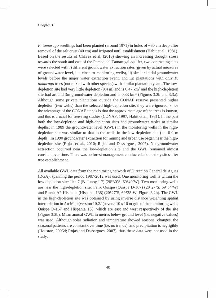
Chapter 3
40
P. tamarugo seedlings had been planted (around 1971) in holes of ~60 cm deep after removal of the salt crust (40 cm) and irrigated until establishment (Habit et al., 1981). Based on the results of Chávez et al. (2016) showing an increasing drought stress towards the south and east of the Pampa del Tamarugal aquifer, two contrasting sites were selected with i) different groundwater extraction rates (given by actual measures of groundwater level, i.e. close to monitoring wells), ii) similar initial groundwater levels before the major water extraction event, and iii) plantations with only P. tamarugo trees (not mixed with other species) with similar plantation years. The low-depletion site had very little depletion (0.4 m) and is 0.47 km2 and the high-depletion site had around 3m groundwater depletion and is 0.33 km2 (Figures 3.2b and 3.3a). Although some private plantations outside the CONAF reserve presented higher depletion (two wells) than the selected high-depletion site, they were ignored, since the advantage of the CONAF stands is that the approximate age of the trees is known, and this is crucial for tree-ring studies (CONAF, 1997; Habit et al., 1981). In the past both the low-depletion and high-depletion sites had groundwater tables at similar depths: in 1989 the groundwater level (GWL) in the monitoring wells in the high-depletion site was similar to that in the wells in the low-depletion site (i.e. 8-9 m depth). In 1990 groundwater extraction for mining and urban use began near the high-depletion site (Rojas et al., 2010; Rojas and Dassargues, 2007). No groundwater extraction occurred near the low-depletion site and the GWL remained almost constant over time. There was no forest management conducted at our study sites after tree establishment. All available GWL data from the monitoring network of Dirección General de Aguas (DGA), spanning the period 1987-2012 was used. One monitoring well is within the low-depletion site: Jica 7 (B. Junoy J-7) (20°30’S, 69°40’W). Two monitoring wells are near the high-depletion site: Felix Quispe (Quispe D-167) (20°27’S, 69°34’W) and Planta AP Hispania (Hispania 138) (20°27’S, 69°38’W, Figure 3.2b). The GWL in the high-depletion site was obtained by using inverse distance weighting spatial interpolation in ArcMap (version 10.2.1) over a 10 x 10 m grid of the monitoring wells Quispe D-167 and Hispania 138, which are east and west respectively of the site (Figure 3.2b). Mean annual GWL in metres below ground level (i.e. negative values) was used. Although solar radiation and temperature showed seasonal changes, the seasonal patterns are constant over time (i.e. no trends), and precipitation is negligible (Houston, 2006d; Rojas and Dassargues, 2007), thus these data were not used in the study.
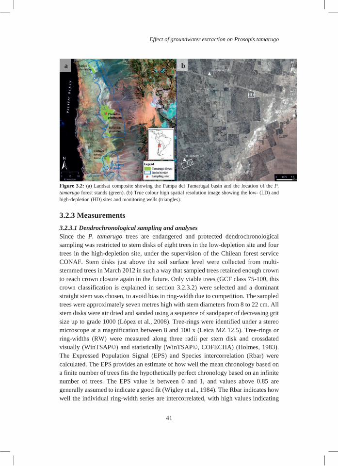
Effect of groundwater extraction on Prosopis tamarugo
41
Figure 3.2: (a) Landsat composite showing the Pampa del Tamarugal basin and the location of the P. tamarugo forest stands (green). (b) True colour high spatial resolution image showing the low- (LD) and high-depletion (HD) sites and monitoring wells (triangles). 3.2.3 Measurements 3.2.3.1 Dendrochronological sampling and analyses Since the P. tamarugo trees are endangered and protected dendrochronological sampling was restricted to stem disks of eight trees in the low-depletion site and four trees in the high-depletion site, under the supervision of the Chilean forest service CONAF. Stem disks just above the soil surface level were collected from multi-stemmed trees in March 2012 in such a way that sampled trees retained enough crown to reach crown closure again in the future. Only viable trees (GCF class 75-100, this crown classification is explained in section 3.2.3.2) were selected and a dominant straight stem was chosen, to avoid bias in ring-width due to competition. The sampled trees were approximately seven metres high with stem diameters from 8 to 22 cm. All stem disks were air dried and sanded using a sequence of sandpaper of decreasing grit size up to grade 1000 (López et al., 2008). Tree-rings were identified under a stereo microscope at a magnification between 8 and 100 x (Leica MZ 12.5). Tree-rings or ring-widths (RW) were measured along three radii per stem disk and crossdated visually (WinTSAP©) and statistically (WinTSAP©, COFECHA) (Holmes, 1983). The Expressed Population Signal (EPS) and Species intercorrelation (Rbar) were calculated. The EPS provides an estimate of how well the mean chronology based on a finite number of trees fits the hypothetically perfect chronology based on an infinite number of trees. The EPS value is between 0 and 1, and values above 0.85 are generally assumed to indicate a good fit (Wigley et al., 1984). The Rbar indicates how well the individual ring-width series are intercorrelated, with high values indicating
a b

Chapter 3
42
high correlations. For time-series analysis the R statistical package dplR (R development Team) was used (Bunn, 2008). Mean chronologies were calculated for both sites (López et al., 2005) and subsequently related to groundwater level and the remotely-sensed Normalized Difference Vegetation Index in winter (NW) and difference of winter and summer Normalized Difference Vegetation Index (NWSD) (explained in Section 3.2.3.2). Detrending was not applied since the time series were too short and statistical modification of the ring-width series would have complicated the comparison with the long-term variation in groundwater level (Grissino-Mayer, 2001). The fast growing rate during the juvenile phase of about 15 years (see Results and Figure B of the Supplementary materials) was excluded from the analysis to avoid the ontogenetic effect. 3.2.3.2. Remote-sensing data 3.2.3.2.1 Landsat - NDVI derived metrics for paraheliotropic plants
P. tamarugo is a paraheliotropic plant, i.e. its leaves adapt their inclination angle to avoid excessive solar radiation and photoinhibition (Ehleringer and Forseth, 1980), as shown in Figure 3.1b. In this way, paraheliotropic plants can photosynthesize longer than normal plants under high solar radiation (Pastenes et al., 2004). At the peaks of solar radiation their leaves fold, avoiding the solar rays and causing a drop in the canopy's spectral reflectance and NDVI (Chávez et al., 2013b; Chávez et al., 2014). These authors showed annual NDVI time series of P. tamarugo stands with peaks in winter and drops in summer, which were negatively correlated to in-situ measured solar radiation (Chávez et al., 2013a; Chávez et al., 2014). Based on this annual behaviour of NDVI, Chávez et al. (2014), proposed new indices for paraheliotropic vegetation: the mean NDVI in winter (NW) as an indicator of annual green biomass (thus expected to decrease over time in case of drought stress) and the NDVI difference between summer and winter (NWSD) as an indicator of the normal paraheliotropic movement and thus an indicator of canopy water content. Trees under drought stress are no longer able to perform paraheliotropic leaf movements, since water is needed for the pulvinus to function, thus the difference between NDVI in winter and summer will be minimal (and therefore lower than in non-drought stressed trees). In addition the NWSD is expected to decrease over time in stressed trees. In this paper, we used both NW and NWSD indices for annual estimations of green biomass and canopy water content of P. tamarugo stands. For the two study sites, all available Landsat 5 TM (Thematic Mapper) and Landsat 7 ETM (Enhanced Thematic Mapper – inclusive the SLC-off scenes) satellite data covering the period 1989-2012 were downloaded from the USGS Earth Explorer website and were considered for use. For the Landsat NDVI time series, cloud-free L1T (orthorectified and geo-referenced) images of 30 m pixel resolution (471 scenes,

Effect of groundwater extraction on Prosopis tamarugo
43
corresponding to path 1 and row 34) were used. The images were pre-processed using the Landsat Ecosystem Disturbance Adaptive Processing System (LEDAPS) to obtain surface reflectance values for all spectral bands (Masek et al., 2006). Finally, the surface reflectance values of the red band and NIR Near Infra-Red (NIR) band were used to compute the NDVI for each date via the following algorithm: NDVI = (NIR-Red)/(NIR+Red). The median NDVI values of all pixels within the plot were calculated. There was no significant seasonal behaviour related to BRDF (bidirectional reflectance distribution function) effects (Chávez et al., 2014). Annual values of NW and NWSD were calculated as average pixel values within both sites:
(1) NW = average of all NDVI scenes from May, June and July (midwinter); (2) NWSD = NW - NS, where NS = average of all NDVI scenes from November, December and January (midsummer). In total, 522 and 367 Landsat pixels were used for the low- and high-depletion sites respectively. To obtain representative values for NS and NW, only years with at least three images in the period June-July-August (midwinter) and November-December-January (midsummer) were used to calculate the average per season (i.e. no intra-annual data, but one value per year).
3.2.3.2.2 Very high spatial resolution (VHSR) satellite images - Green Canopy Fraction (GCF).
At the single tree level, other indicators derived from satellite data can be used as drought indicators. Via high spatial resolution satellite images, the Green Canopy Fraction (GCF) from individual P. tamarugo trees can be obtained (Chávez et al., 2016). It has been shown that drought stress causes P. tamarugo to loose canopy over time (Chávez et al., 2013b), thus GCF is expected to decrease. The GCF values provide information on the status of the crown viability (an indirect measurement of photosynthetic activity) at tree level. The GCF was calculated as the ratio of green to brown parts of the canopy (green canopy/(green + brown canopy)) assessed from four angles at ground level (digital photos) and was related to the spectral signal of a Worldview2 image of 2 m pixel resolution from July 2011. Single tree canopies were delineated with a Quickbird2 image in summer (to avoid crown shadows) with a 0.6 m pixel resolution (Chávez and Clevers, 2012). The GCF was divided into four classes (each of 25%), starting with the class < 25%, which represents trees with a very dry canopy. 3.2.4 Statistical analyses 3.2.4.1 Stand level variables (GWL, NW, NWSD, RW) For the stand level comparison, the Mann-Kendall trend (MKT) test as suggested by Hipel and McLeod (1994) and later by De Beurs and Henebry (2005) was used to

Chapter 3
44
check for significant trends on the monotonic series of annual GWL (expressed in negative values), annual RW, NW, NWSD. Temporal stationarity was accomplished in most cases, as shown by the autocorrelation function (ACF as implemented in the R package). The only significant autocorrelation found was for the GWL series for the high-depletion site and for time lags of < 4 years. Association between different time series was analysed by the Kendall rank correlation (KRC). The analysis was performed using the Kendall package of R and significance levels of 0.01, 0.05 and 0.1 were shown. Additionally differences between the mean values of each parameter (RW, NW, NWSD and GWL) per site were calculated, using all annual time steps as single replicates and assuming independent samples as shown by the ACF function. Since some of the parameters were not normally distributed the non-parametric Mann-Whitney U test (using IBM SPSS Statistics 22 software) was used for all parameters to compare the variables at each site. 3.2.4.2 Single tree variables (GCF) GCF was used to describe the cumulative effect of drought stress on the amount of remaining green canopy of single trees at both high-depletion and low-depletion sites. For this variable the nonparametric Mann-Whitney U test was also used to test differences between the GCF values at the two sites using single trees as replicates.
3.3 Results 3.3.1 Groundwater level The GWL dropped by 0.4 m in the low-depletion site (data available for 1987-2012) and ~3 m in the high-depletion site (data available for 1989-2012). While the decreasing trend of the high-depletion site was highly significant (p < 0.01), the significant decreasing trend in the low-depletion site was less strong (p < 0.05), as shown by the Mann-Kendall trend test (i.e. the decreasing trend of the high-depletion site was more evident). The GWL of the high-depletion site was significantly lower than the low-depletion site (U < 0.001; Z = -6.059; p < 0.001) according to the Mann-Whitney U test. 3.3.2 Annual ring-width and groundwater level (stand level) Although the P. tamarugo tree forms distinct rings with the ring boundaries marked by narrow bands of marginal parenchyma (Figure 3.1c), the rings are frequently difficult to discern for various reasons: intra-annual density variations, discontinuous parenchyma bands, or extremely narrow rings, as seen in other tree species (Decuyper et al., 2014). The number of rings detected in the 12 trees investigated ranged from 34 to 39, which is consistent with the estimated age of ca. 41 years (the trees were planted

Effect of groundwater extraction on Prosopis tamarugo
45
around 1971). As a consequence of the planting method (seedlings of 3-5 months old were planted in 60 cm deep holes below the current soil surface level) (Lanino, 1972), some of the rings from the time series are not visible in our disks since they are only apparent at the base of the tree (i.e. 60 cm below the soil surface level) explaining the lower number of rings found in this study. The number of tree-rings also supports the assumption that the detected rings are annual, as the number of rings did not exceed the estimated age. Ring-width series measured from different radii of the same tree crossdated well. In some cases, crossdating was obscured by reaction wood formation, especially in the outermost part of the stem. For this reason, the outermost stem parts of the disks, where annual ring boundaries could not be discerned with confidence, were left out of the chronology to avoid introducing possible errors (the rest of the chronology was used and crossdated). Tree-ring series of trees from the two sites showed similar annual variation, with slightly better intercorrelation between trees growing in the low-depletion site (EPS = 0.96; Rbar = 0.79) than between trees growing in the high-depletion site (EPS = 0.83; Rbar = 0.57). All P. tamarugo trees exhibited a similar growth trend, with fast juvenile radial growth during the first 10-15 years (which was excluded from the statistical analysis), followed by a sharp reduction to a persistently lower and stable average growth rate of approximately 1 mm per year. From 1987 to 2012, average annual RW had a significant negative trend over time in trees in both sites, with p < 0.01; MKT = -0.520 for the low-depletion site and p < 0.01; MKT = -0.586 for the high-depletion site. This is partly attributable to the remaining small ontogenetic trend in all ring-width series. Nevertheless, a comparison between the ring-width chronologies of both sites (Figure 3.3d) showed that the ring-width (i.e. the whole time series minus the juvenile phase) was significantly lower by 48% in the high-depletion site compared to the low-depletion site (U = 135; Z = -3.715; p < 0.001).

Chapter 3
46
Figure 3.3: Time series of stand level variables: (a) Groundwater level (GWL) in metres below ground level.; (b) NDVI in winter (NW) The blue arrows represent the few rainfall events (ranging from 1.6 to 6.9 mm per year) and could explain the small peaks in NW; (c); NDVI difference between winter and summer (NWSD). (d) Average annual ring-width (RW) of viable P. tamarugo trees, where mean radial growth was 48% less in the high-depletion site.
a
b
d
c

Effect of groundwater extraction on Prosopis tamarugo
47
3.3.3 NDVI metrics (NW and NWSD) and groundwater level (stand
level) The time-series analysis for the NW showed significant trends for both sites (Table 3.1) as indicated by the Mann-Kendall trend (MKT) test. In the low-depletion site, NW increased over time (p < 0.01; MKT = 0.557), while, in the high-depletion site, NW declined over time (p < 0.01; MKT = -0.747; Figure 3.3b). The NW was significantly lower when comparing the high-depletion site with the low-depletion site (U = 20.5; Z = -5.361; p < 0.001). NWSD showed no significant positive or negative trend over time in the low-depletion site but a negative trend in the high-depletion site (p < 0.01; MKT = -0.573) (Fig 3.3c). However, when comparing NWSD there were no differences between the two sites (U = 230.5; Z = -0.012; p = 0.990).
In the low-depletion site, the Kendall rank correlation (KRC) indicated that the correlation with the GWL was significantly negative for the NW (p < 0.05; KRC = -0.352) and poor for the NWSD (p < 0.1; KRC = -0.305). In the high-depletion site, a more significant and positive correlation was found between NW and GWL (p < 0.01; KRC = 0.688), and NWSD and GWL (p < 0.01; KRC = 0.482), (Table 3.1).
Table 3.1: Trends and correlation between stand level variables: groundwater level (GWL, expressed in negative values), ring-width (RW), NDVI measured in winter (NW), and NDVI difference between winter and summer (NWSD) of P. tamarugo sites subject to low and high groundwater depletion.

Chapter 3
48
3.3.4 Annual ring-width and NDVI metrics (NW and NWSD)
(stand level) The significant negative correlation between RW and NW (p < 0.01; KRC = -0.399) in the low-depletion site might be somewhat explained by the slight ontogenetic effect in the RW(see Figure B in the Supplementary materials), yet there was no correlation between RW and NWSD. Although this ontogenetic effect in the RW is similar in the high-depletion site, there is a significant positive correlation between RW and both NDVI-derived parameters (NW: p < 0.01; KRC = 0.420 and NWSD: p < 0.01; KRC = 0.457).
3.3.5 Green Canopy Fraction and groundwater level (tree level)
Although all GCF classes appear in both sites in 2011 (Figure 3.4), more trees in the high-depletion site fall within lower GCF classes. There is little difference between sites in the fraction of trees in the lowest GCF class (GCF = 0-25) but in the high-depletion site there are 11% more trees in GCF class 25-50 than in the low-depletion site (Table 3.2). Only 8% of the trees in the high-depletion site were in GCF class 75-100, compared with 15% in the low-depletion site. The average GCF of all individual trees summarizes the overall difference in GCF between the two sites, which was 0.470 for the high-depletion site and 0.549 for the low-depletion site, and there was a significant difference in GCF values between sites (U = 1522603.5; Z = -8.404; p < 0.001). The standard deviation of GCF was higher in the low-depletion site (i.e. 0.519) than in the high-depletion site (Table 3.2). In addition to the numerical differences, there are different spatial patterns in the low-depletion site (i.e. the band of trees with a GCF < 0.25 and 0.25 to 0.50); in the high-depletion site the GCFs are more homogenous (Figure 3.4).

Effect of groundwater extraction on Prosopis tamarugo
49
Figure 3.4: Green Canopy Fraction (GCF) derived from high-resolution (2.4 m pixel resolution) Worldview2 satellite data (acquired in July 2011). Table 3.2: Forest site characteristics of the two study sites. The Green Canopy Fraction (GCF) classes show the percentage of trees organized in four GCF classes. GCF per tree was calculated using the Worldview2 image of July 2011.
3.4 Discussion 3.4.1 Radial stem growth of viable trees is affected by groundwater
depletion Radial growth in the high-depletion site was significantly lower than in the low-depletion site by 48%. The generally slow growth may conceal even greater differences in resource availability between the two sites, In addition, since only viable trees with a GCF class of 75-100 could be sampled for ring-width analyses, it
Site Low-depletion site High-depletion site
CONAF site Recreo España
Year planted 1971 1971
Number of trees 2364 1532
Tree density (per ha) 50.3 46.4
Average GCF* (SD) 0.549 (0.519) 0.470 (0.185)
GCF class < 25 (%) 9 11
GCF class 25−50 (%) 38 49
GCF class 50−75 (%) 37 32
GCF class 75−100 (%) 15 8

Chapter 3
50
is most likely that overall growth is even lower, as less viable trees have even less growth. A reduction in ring-width was also found in other arid ecosystems where water was limiting growth: for example for Populus trichocarpa and Pinus jeffrey (Stromberg and Patten, 1990) and for P. flexuosa DC. (Giordano et al., 2011). The reduction in ring-width in the high-depletion site may be related to a shift in allocation patterns towards investment of resources into root elongation (Chaves et al., 2003; Markesteijn and Poorter, 2009; Micco and Aronne, 2012). Another possible cause of reduced growth might be reduced carbon fixation due to longer periods of stomatal closure (Mcdowell et al., 2008). Groundwater depletion may lead to amplification of this potential allocation effect, as seen from the reduced ring-width of the viable trees in the high-depletion site (Figure 3.3d). All trees showed high radial growth during the first 10-15 years after establishment. Such a juvenile phase with high height and radial growth is in line with results reported by Rivera et al. (2010), who studied P. tamarugo trees in the same region, and by Alvarez et al. (2011) and Villagra et al. (2005) in P. flexuosa growing under similarly hyper-arid conditions. In its natural habitat, P. tamarugo trees germinate after major floods which occasionally occur as a result of runoff from the Andes (Mooney et al., 1980). The fast juvenile growth can be an adaptation of these trees to quickly establish and reach the groundwater and in this way avoid premature desiccation when the flood event is over and the high solar radiation prevails (Salih, 1998; Sudzuki, 1985b). Once the tree roots reach the groundwater, allocation strategies may change, with more biomass being invested in maintaining foliage and with root increment being stimulated by drought stress (Markesteijn and Poorter, 2009). Carbon allocation or limited carbon fixation may be the explanation of the relatively low radial increments in the last 20 years in both sites (Figure 3.3d). However, further research is needed to understand carbon allocation strategies or limitations in carbon fixation of P. tamarugo trees under drought stress. 3.4.2 Increased drought stress due to groundwater depletion - the
remote sensing (crown) perspective The significant reduction in NW and NWSD of groundwater-dependent P. tamarugo trees in the high-depletion site indicates that the trees are experiencing increasing drought stress as a consequence of groundwater depletion. The high evaporative demand in desert areas induces drought stress once the water supply drops below a certain threshold (Houston, 2006d). The lower NW and NWSD in the high-depletion site indicate that a drop in groundwater level of about 3 m over the last two decades induced increased drought stress in tree crowns throughout the forest site. The positive correlation between NW, NWSD and GWL could be another indicator showing the detrimental effects of this depletion intensity. Furthermore, the groundwater level in

Effect of groundwater extraction on Prosopis tamarugo
51
the high-depletion site dropped to 12 m, which according to Chávez et al. (2016) is within the zone (12-20 m) in which a disruption of the water status of the tree occurs. This indicates that most P. tamarugo trees in the high-depletion site have had limited access to water (Chávez et al., 2016). In the low-depletion site, the positive trend in NW suggests that most trees continued to increase their green biomass over time, which is also supported by the negative correlation between NW and GWL (i.e. NW increases due to crown growth, while almost no change is seen in the GWL). The absence of a significant trend in NWSD points to the absence of excessive drought stress, which implies well-functioning pulvinar movement of the leaves during summer (Chávez et al., 2014). In line with this, GCF was lower in the high-depletion site. A GCF class below 50 indicates trees are unhealthy (Chávez et al., 2016) and 49% of the trees in the high-depletion site belonged to this category (Table 3.2). Although the GCF is considerably higher in the low-depletion site, the large standard deviation indicates that in addition to healthy trees (high GCF), stressed trees (low GCF) are also present in the tree community here. This, together with the observation of clear spatial patterns in the low-depletion site (Figure 3.4), could point to the presence of below-ground features (e.g. bedrock) which define local water availability, e.g. the presence of impenetrable layers or layers hampering root expansion to greater depths to follow the falling groundwater level. Reduced crown vitality (GCF) also means reduced carbon assimilation for root growth and in turn reduces the tree's ability to access declining water reserves. This could also imply that under prevailing drought stress, radial growth is restricted. 3.4.3 Impact of groundwater depletion on P. tamarugo All the indicators investigated - GCF, NW, NWSD, and RW - point to a strong effect of groundwater extraction on the viability of the groundwater-dependent P. tamarugo tree. Viable trees seem to cope relatively well with falling GWL, but the GCF values show that most of the P. tamarugo trees in the high-depletion site were affected by the drop of about 3 m in GWL in the last two decades. This indicates that there is a certain critical threshold of GWL, below which photosynthesis, maintenance of growth and adaptation of root length are constrained. A recent study by Chávez et al. (2016), assessed the GWL of the entire Pampa del Tamarugal and suggested the critical threshold for P. tamarugo survival was a depth of 20 m. It is known that other Prosopis species can reach groundwater as deep as 50 m (Phillips, 1963). However, when evaluating the adaptive capacity of a species, different factors play an important role, such as initial GWL, extent and speed of GWL depletion, site fertility and impenetrable layers. Our findings suggest that most trees in the high-depletion site are beyond their adaptive capacity and showed signs of stress at a GWL of ~12 m, which is in line with conclusions of Chávez et al. (2016), who showed signs of disruption of
Chapter 3
52
the water status in the P. tamarugo at this depth. If the current situation remains stable, or GWL continues to fall in response to anthropogenic (pumping) or natural causes, the population will decline. It is clear that the current extraction limitation of 4000 l/s in the Pampa del Tamarugal aquifer is too high for the natural recharge rate of 976 l/s (JICA-DGA-PCI, 1995; Rojas and Dassargues, 2007). Other factors in addition to the anthropogenic pressure that could cause serious and immediate impacts on the P. tamarugo population are severe drought and earlier snowmelt or rainfall instead of snow (thus releasing water faster and causing shortages in groundwater supply later in the summer season) in the Andes mountains, due to higher temperatures as described in Coudrain et al. (2005). 3.4.4 Applicability of a multi-scale approach in arid environments With this multi-scale approach, the impact of groundwater extraction on groundwater dependent forests was assessed and a methodology for studying the effects on resource acquisition (canopy) and radial growth was demonstrated. Although only one very high-resolution satellite image for deriving data at tree level (GCF) was used, the results show the potential of this approach for future studies. For example, the increasing use of drones and the upcoming high spatial and/or temporal resolution satellites with higher spectral resolution, such as Worldview3 (spatial resolution of 2 m and eight spectral bands) and Sentinel 2 (free access, spatial resolution: 10 m and five days' revisit time) will increase possibilities to study ecosystems throughout the year and to combine this data with ground-based measurements at tree level. Arid ecosystems have the advantage of being infrequently covered by clouds, which leads to more cloud free and higher quality (e.g. less aerosols) satellite data, as was the case in the Atacama Desert. To date, the combination of remotely-sensed indices with dendrochronology of tropical trees has not been sufficiently explored. One of the few studies showed that shifts in regional precipitation patterns could be explained by combining tree-ring chronologies and remotely-sensed data (Southworth et al., 2013a). In the present paper, the results provided insight into what can be seen from the canopy and within the tree (i.e. radial growth) in trees undergoing drought stress (see Table 3.1, NW, NWSD and RW).

Effect of groundwater extraction on Prosopis tamarugo
53
3.5 Conclusions We conclude that P. tamarugo trees were affected by the drop in groundwater of about 3 m (from ~8 to 12 m) in recent decades. Groundwater depletion increases drought stress in the tree canopy and reduces radial growth, even in viable trees. Although viable trees can currently cope with this level of groundwater depletion, they could experience a reduction carbon fixation or may allocate more resources towards root elongation in order to remain in contact with the groundwater (this could be a possible explanation of the higher reduction in radial growth in the high depletion site). Furthermore, the drought-stress symptoms, detected by GCF on tree level, and NW and NWSD on stand level in the high-depletion site suggest that the viability of this whole stand is declining. If groundwater extraction continues in the Atacama Desert at the same rate, this unique tree species may not persist. In order to curb this trend, groundwater extraction rates should decrease drastically or should be spread both spatially and temporally so that the P. tamarugo stands have more time to adjust to lower soil water levels. The combination of remote sensing and tree-ring analysis provides a relevant insight into the ecophysiology of this desert tree, by assessing crown and stem status, and shows potential for upscaling drought effects from trees to stands and perhaps basins.
Acknowledgements We thank the Alberta Mennega foundation, Beca CONICYT Wageningen, and Fondo Basal FONDECYT FB-002 (linea 4) for providing financial support. We are grateful to the Ministry of Agriculture - CONAF (Government of Chile) for granting access to the sites, Mauricio Ortiz for his valuable knowledge on leaf phenology, Cristian Riquelme for logistic support, and the Universidad Arturo Prat for providing climatic data from the Canchones experimental station. The discussion improved from exchange of ideas with colleagues from the COST FP1106 network. We are indebted to Digital Globe for the Quickbird2 and Worldview2 imagery and to NASA for the Landsat images. We are also grateful to the editor Cristina Armas, the anonymous reviewers and Sarah Carter for their useful remarks improving the paper. Professional language editing was provided by Joy Burrough.

54

55
Chapter
4 2 Spatio-temporal assessment of beech growth in
relation to climate in Slovenia – An integrated approach using remote sensing and tree-ring
data
M. Decuyper, R.O. Chávez, S.A. Estay, K. Čufar, P. Prislan, J. Gričar, Z. Črepinšek, M. Merela, M. de Luis, R. Serrano Notivoli, E. Martinez del Castillo, J.G.P.W.
Clevers, D.M.A. Rozendaal, F. Bongers, M. Herold, U. Sass-Klaassen Predicted climate changes are likely to affect tree growth and biomass production specifically through increased frequency and intensity of droughts, heat waves, and frosts. Yet, there is still a lot of uncertainty on how trees respond to these changes. Growth measurements such as ring width are based on single locations, and for scaling up, the link between ring width and remote sensing needs to be understood. Linking ground-based wood increment to remotely sensed data has only been done in a few studies, often not taking the climatic drivers into account. We used tree-ring data and crown characteristics derived from the Moderate Resolution Imaging Spectroradiometer (MODIS) to assess the effect of general climate conditions as well as extreme climate events on the growth of beech (Fagus sylvatica L.) in Slovenia. Surprisingly, we did not find a consistent relationship of specific climate factors with tree-ring width nor with remotely sensed plot variables (e.g., the Enhanced Vegetation Index; EVI) across the study sites. Only severe, large scale damage of the canopy could be detected in both tree-ring width and remotely sensed EVI variables, as was the case for the ice storm in 2014. The large unexplained variation between climate, ring width (RW), and remotely-sensed variables suggests that non-climatic factors related to site and stand characteristics such as soil moisture and species composition determined variation in beech growth. The weak correlation between RW and remote

Chapter 4
56
sensing indices might result from various factors: (i) the 250 m MODIS spatial resolution pixels might contain a mixture with less drought-prone tree species, overall leading to little canopy damage; (ii) little overlap between the different time series, as remote sensing data was available for the last 16 years, but in the ring-width series recent years were often missing; (iii) it is possible that there is no relationship between remote sensing EVI indices, climate and RW, because RW represents stem growth and EVI is a proxy for canopy greenness. Future research should focus on a better understanding of climate-growth relationships, by closely linking ecophysiological research and high resolution remote sensing data. Keywords Climate extremes; dendrochronology; ice storm; drought
4.1 Introduction Many studies indicate that at Northern latitudes the effect of climate change (i.e. warming due to increasing CO2 levels) prolongs the growing season of trees (Badeck et al., 2004; Menzel, 2002; Nabuurs et al., 2002; Nemani et al., 2003). Although increasing CO2 levels enable trees to use water more efficiently, their growth and biomass production may be curbed by increased climate-induced water shortage (Bréda et al., 2006; Fonti et al., 2013), heat stress (Bréda et al., 2006; Ciais et al., 2005), or increased respiratory demands (Mcdowell et al., 2008). Photosynthetic activity determines the amount of carbohydrates available for wood formation. Thus, leaf phenology is intrinsically linked to wood formation (through cambial phenology). Summer droughts are common in Atlantic Europe and are known to reduce wood formation (i.e. tree-ring width) for species such as Scots pine (Pinus sylvestris L.) (Gruber et al. 2010) and beech (Fagus sylvatica L.) (Ciais et al., 2005; Čufar et al., 2008a; Giagli et al., 2016; Prislan et al., 2013; Scharnweber et al., 2011; van der Werf et al., 2007). However, recent studies indicated that precipitation was not a limiting factor in ring width (from here on: RW) (Prislan et al., 2018), while Van der Werf et al. (2007) found that RW increment ceased during the 2003 drought, but recovered in the same year. Similarly, variable effects of air temperature on ring width have been found, with negative air temperature effects on growth in different months (Čufar et al., 2008b; Di Filippo et al., 2007; Fischer and Neuwirth, 2013; van der Werf et al., 2007).The impact of expected climate changes on tree growth depends on the interplay of climate factors, as well as the timing of the occurrence of the climatic events and the interaction with specific site conditions. Therefore, the inclusion of multiple data types (i.e. RW and climate parameters) is needed to better understand effects of climatic events (Norman et al., 2016).

Spatio-temporal assessment of beech growth in relation to climate in Slovenia
57
Some measurement techniques for tree growth focus on the measurement of stem growth of individual trees, like dendrochronology, while other techniques focus on the measurement of the total biomass of trees or even forest stands (i.e. at the plot level), like remote sensing techniques (Avitabile et al., 2015). While tree-centred measurement methods such as dendrochronology and xylogenesis are important tools to assess and understand (long-term) climate-growth relationships, they are time-consuming and costly, which makes it difficult to monitor many locations. Furthermore, local effects of climate or soil characteristics can make them unrepresentative for large-scale assessments (Norman et al., 2016). Therefore, remote sensing can play an important role in tree-growth monitoring by upscaling from the individual tree level to larger scales in order to map areas that might be under threat given the climate change predictions. Several studies indicated the ability of remote sensing indices to detect drought or heat waves (Hlásny et al., 2015; Vicca et al., 2016). However, due to the relatively coarse spatial resolution of the sensor (30 - 250 m for sensors that have longer time series available), each grid cell represents an average of different tree species, unless large, homogeneous forest patches are present (Deshayes et al., 2006). Furthermore, from space the canopy greenness as a proxy for the tree’s productivity is measured, but until now few studies attempted to link tree-ring width (stem) with remote sensing derived indices (Babst et al., 2018; Bunn et al., 2013). Yet, it is not clear how remotely sensed indices obtained from chlorophyll pigments in the leaves and the amount of leaves relate to actual wood formation (i.e. tree-ring width). A relationship between both measuring techniques would allow for upscaling ground-based point measurements conducted on single trees to stand level. In this study, we assess the general effect of climate factors, and to some extent climate extremes, on the growth of beech in Slovenia, both from a tree-ring width (stem) as well as from a remote sensing (canopy) perspective. Although the distribution range of beech has been increasing recently, the species is affected by adverse climate effects, like ice damage, late frosts, heat waves and droughts (Marenče, 2015; Slovenian Forest Service, 2015). Secondly, we quantify the relationship between tree-ring width and remote sensing derived variables, and we aim to upscale the results from ground-based RW measurements to remote sensing derived canopy measurements. Specifically, we ask:
- How do climate variables (and climate extreme events) affect beech radial growth (tree-ring width) and canopy characteristics (EVI indices) at different sites across Slovenia?
- Can we link tree-ring width measurements with remote sensing derived variables and upscale from tree level to plot or even national level?
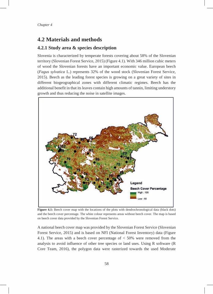
Chapter 4
58
4.2 Materials and methods 4.2.1 Study area & species description Slovenia is characterized by temperate forests covering about 58% of the Slovenian territory (Slovenian Forest Service, 2015) (Figure 4.1). With 346 million cubic meters of wood the Slovenian forests have an important economic value. European beech (Fagus sylvatica L.) represents 32% of the wood stock (Slovenian Forest Service, 2015). Beech as the leading forest species is growing on a great variety of sites in different biogeographical zones with different climatic regimes. Beech has the additional benefit in that its leaves contain high amounts of tannin, limiting understory growth and thus reducing the noise in satellite images.
Figure 4.1: Beech cover map with the locations of the plots with dendrochronological data (black dots) and the beech cover percentage. The white colour represents areas without beech cover. The map is based on beech cover data provided by the Slovenian Forest Service. A national beech cover map was provided by the Slovenian Forest Service (Slovenian Forest Service, 2015) and is based on NFI (National Forest Inventory) data (Figure 4.1). The areas with a beech cover percentage of < 50% were removed from the analysis to avoid influence of other tree species or land uses. Using R software (R Core Team, 2016), the polygon data were rasterized towards the used Moderate

Spatio-temporal assessment of beech growth in relation to climate in Slovenia
59
Resolution Imaging Spectroradiometer (MODIS) 250 m grid size (see section 4.2.4). Only 250 m pixels with ≥ 50% beech were included in this study. 4.2.2 Dendrochronological data Dendrochronological ring width (RW) data for 25 sites were included (Figure 4.1) from previous studies (e.g. Čufar et al., 2008; Prislan, 2018; Prislan et al., 2013). Samples varied from 2 - 32 trees per site, with 3 cores at different orientations taken per tree. The age of the sampled trees ranged from 61 to 271 years; however, RW data was only considered for the period between 2000 – 2016 in the analysis. RW time series have variable length (Figure 4.2). Detailed descriptions of sampling and sample preparation can be found in Čufar et al. (2008); Prislan et al. (2018); Prislan et al. (2013).
Figure 4.2: Tree-ring replication per site between the years 2000 and 2016. To correct for ontogenetic effects, i.e. decreasing ring width with increasing tree age, all raw dendrochronological data together were standardized using regional curve standardizations in the ARSTAN 6.05P programme (Cook, 1985). The RW of the individual trees was averaged per plot. All plots were taken into account in this study, but three particular plots, Javorniki, Idrija and Masun were used to exemplify the effect of most recent extreme weather events. These sites were selected since they had the most recent RW data and we know that they were affected by the 2014 ice storm, with Masun being the least affected (Slovenian Forest Service, 2015).
0
5
10
15
20
25
30
Num
ber o
f site
s
Year
Chapter 4
60
4.2.3 Climate data and model Daily precipitation and average temperature grids were generated using 36 weather stations covering the whole study area. The stations ranged in altitudes from 2 to 2514 m.a.s.l. and had on average 4.71% missing data in the period 2000-2016. The reconstruction of each station was made in two steps: (1) we flagged and removed unreliable records, and (2) we filled in missing values based on the filtered dataset resulting from the previous step as follows. A grid was created with a cell size of 250 meters in order to match the MODIS resolution. To obtain estimated values of temperature for each grid cell, multivariate logistic regressions (MLR) were used to compute reference values using altitude, latitude, and longitude as covariates. Daily precipitation for each point of the grid was estimated using two reference values based on the 10 nearest observations on the corresponding day: i) a binomial prediction referred to the probability of occurrence of a wet day and, ii) a magnitude prediction referred to the amount of precipitation using MLR. The reconstructed precipitation was calculated using the “reddPrec” package in R statistical software (http://cran.r-project.org). From the climate grids, three climate variables were calculated: CDD (the number of consecutive days where precipitation was <1 mm during the growing season, a proxy of drought intensity); Prec (the total precipitation during the growing season) and Tmax (the absolute maximum temperature during the growing season, a proxy of heatwaves causing the burning or browning of the leaves). We did check for a proxy in the climate data for ice storms, but we could not capture the ice storm with the available climate data. 4.2.4 Remote-sensing data The entire 16-days MODIS vegetation indices catalogue from the Terra (product MOD13Q1) and Aqua (MYD13Q1) satellites was used in this study. These satellites acquire images from the whole Earth on a daily basis and, in order to avoid data gaps due to clouds and other atmospheric contamination, they are composed within a temporal window of 16 days. These composites provide a more complete spatial coverage, which is especially useful for cloudy areas. From this product, two vegetation indices are available: the Normalized Difference Vegetation Index (NDVI) and the Enhanced Vegetation Index (EVI), from which the EVI was selected in this study since it has proved more sensitive than NDVI to detect leaf phenological changes for high biomass vegetation like beech forests (Huete et al., 2002; White et al., 2014). Combining the MODIS Terra and Aqua satellite data, a time series of 768 MODIS EVI layers was obtained, spanning from 2000 till 2016. Since the (Vegetation Index) VI algorithm of each of the two satellites generates a 16-day composite, and they are eight days apart, we have a time series with a temporal resolution of 8 days.

Spatio-temporal assessment of beech growth in relation to climate in Slovenia
61
All the scenes were pre-processed using the quality flags provided within the MODIS vegetation indices product using the 'raster' package as implemented in the R software (R Core Team, 2016). Based on these quality flags, all pixels with clouds, cloud shadows, water, snow, ice, and images with a high level of aerosols were neglected.
Vegetation disruptions were detected using EVI anomalies (Figure 4.3). For each 250 x 250 m pixel, the EVI time series for the period 18-02-2000 till 19-12-2016 was extracted, resulting in a 768 time step series in the most favourable case (e.g. no clouds or cloud shadows) (Figure 4.3a). The time series were sorted by the day of the year (DOY) per year to calculate the reference phenological curve (Figure 4.3b). Using all available EVI values (i.e. 46 per year), the maximum probability of having a given EVI value at a given DOY was calculated (dark red line in Figure 4.3c). Probabilities of having certain EVI values at different DOY were calculated using the 'rts' package as implemented by the R software (R Core Team, 2016).
An iterative leave-one-out process was applied where a given year (e.g. 2014, Figure 4.3) is left out and the reference annual phenological cycle is then estimated using the remaining years (Figure 4.3b). Then, the EVI anomaly for the given year is calculated by subtracting the reference values from the measured values of that year. Positive EVI anomalies show a “greening” of the vegetated land surface while negative anomalies show a “browning”. All pixels of Slovenia together provide a national EVI anomaly map and 46 anomaly maps were obtained per year, i.e. 768 maps for the period 2000-2016.
Since the aim is to relate the anomaly data with annual RW data, the 8-day resolution EVI anomaly data under the reference line was summed up to obtain the area under the curve (EVI_AUC) per year. Only negative anomalies were used to calculate this variable. Furthermore, the absolute minimum was derived to detect potential extreme events (EVI_Min). These calculations were based on the growing season of the tree (i.e. March-October).

Chapter 4
62
Figure 4.3: Calculation of the Enhanced vegetation index (EVI) anomaly for a single 250 m pixel of Fagus sylvatica forest. (a) The full time series of 16-day composites of EVI values is extracted for the given pixel (illustrated using Terra only). The black box shows the growing season 2014 (a year with a severe ice storm) to be analysed. (b) The EVI values from all growing seasons (grey x), except for the growing season to be analysed (2014 in black circled dots), are used to calculate the reference EVI curve (showing the seasonal behaviour of this deciduous tree). (c) The probability (red and yellow shades) of an EVI value occurring at a given day of the year is calculated: the dark red line (maximum probability) shows the reference EVI phenological curve for this forested pixel. The difference between the dark red line (reference) and the black dots (measured values), the EVI anomaly (black arrow), is then used to account for a disruption.
4.2.5 General approach In order to be able to overlay or relate the datasets, the beech cover map and the climate data were resampled to match the 250 m resolution of the MODIS data. Around the plot locations, a buffer of 5 km was made assuming similar climate conditions. In this way the overlap with the MODIS pixels was not only based on one pixel (see detailed flowchart – Figure 4.4).
a)
b) c)
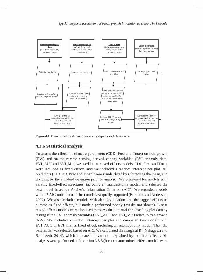
Spatio-temporal assessment of beech growth in relation to climate in Slovenia
63
Figure 4.4: Flowchart of the different processing steps for each data source. 4.2.6 Statistical analysis To assess the effects of climatic parameters (CDD, Prec and Tmax) on tree growth (RW) and on the remote sensing derived canopy variables (EVI anomaly data: EVI_AUC and EVI_Min) we used linear mixed-effects models. CDD, Prec and Tmax were included as fixed effects, and we included a random intercept per plot. All predictors (i.e. CDD, Prec and Tmax) were standardized by subtracting the mean, and dividing by the standard deviation prior to analysis. We compared ten models with varying fixed-effect structures, including an intercept-only model, and selected the best model based on Akaike’s Information Criterion (AIC). We regarded models within 2 AIC-units from the best model as equally supported (Burnham and Anderson, 2002). We also included models with altitude, location and the lagged effects of climate as fixed effects, but models performed poorly (results not shown). Linear mixed-effects models were also used to assess the potential for upscaling plot data by testing if the EVI anomaly variables (EVI_AUC and EVI_Min) relate to tree growth (RW). We included a random intercept per plot and compared two models with EVI_AUC or EVI_min as fixed-effect, including an intercept-only model. Then the best model was selected based on AIC. We calculated the marginal R2 (Nakagawa and Schielzeth, 2014), which indicates the variation explained by the fixed effects. All analyses were performed in R, version 3.3.3 (R core team); mixed-effects models were
Dendrochronological
data(Raw tree-ring width)
Datatype: points
Remote sensing data(Modis EVI layers)
Datatype: raster (250m resolution)
Climate data(Daily temperature and
precipitation data)Datatype: points
Beech cover map(Percentage beech cover)
Datatype: polygon
Data standardization Data quality filtering Data quality check and gap filling
Resampling to 250m raster
Model temperature and precipitation over a 250m
raster using altitude, latitude and longitude as
covariates
EVI anomaly maps (Area under the curve and absolute minimum)
Creating a 5km buffer around the point centre
Average of the EVI anomaly pixels within the
5km buffer and with beech cover > 50%
Average of the climate variables pixels within the
5km buffer and with beech cover > 50%
Deriving CDD, Tmax and Prec over the growing
season

Chapter 4
64
run using the “lme4” package (Bates et al., 2014), the marginal R2 (R2m) was calculated using the package “MuMIn” (Nakagawa and Schielzeth, 2014).
4.3 Results 4.3.1 Effect of climate on the growth of beech 4.3.1.1 The dendrochronological perspective The best model (Model 3, Table 1) included Prec and Tmax and their interaction, indicating negative effects of Prec and Tmax on RW (Figure S4.1). This means that RW decreased with higher maximum temperatures and higher precipitation volumes. However, the amount of variation that was explained by this model was very low (R2m = 0.10). Table 4.1: Overview of the different mixed effect models used to compare the effect of climatic parameters. Mixed model outputs are shown with their AIC value to test the effect of climate variables on RW, EVI_AUC and EVI_Min.
Model Fixed effects AIC (RW)
AIC (EVI_AUC) AIC (EVI_Min)
1 CDD + Prec + Tmax 24.31 0.00 0.00 2 CDD + Prec * Tmax 5.57 15.59 8.15 3 Prec * Tmax 0.00 10.37 10.16 4 Prec + Tmax 19.28 26.02 18.40 5 CDD + Prec 15.79 27.08 18.46 6 CDD + Tmax 16.76 32.07 29.38 7 CDD 7.87 39.36 34.90 8 Prec 10.43 36.11 25.11 9 Tmax 11.66 41.44 36.41 10 intercept only 2.52 48.32 43.13
Although year to year climate variables were not strongly correlated to RW, years with extreme climate conditions (i.e. drought of 2003 and ice storm of 2014) did show a decrease in RW (Figure 4.5). The averaged RW time series for three sites (i.e. Javorniki, Idrija, Masun) were known to be affected by the 2014 ice storm (Slovenian Forest Service, 2015) (Figure 4.5a). Besides the lower ring width in 2014, there was also a reduction in RW in the year 2003 (drought), 2011 (drought and heat wave), 2013 (heat wave), 2015 (drought and heat wave). Similar patterns in RW were found when taking all sites into account, although the larger standard deviations indicate large site-to-site variation (especially in 2003 - Figure 4.5b). RW decreased over time for each of the three sites and all sites combined. Although not statistically proven,

Spatio-temporal assessment of beech growth in relation to climate in Slovenia
65
the decrease in RW could have resulted from the frequent extreme events from 2011 onwards (Figure 4.5).
Figure 4.5: ( a) Average RW and EVI_AUC with standard deviation of the three sites (i.e. Javorniki, Idrija, Masun), which are known to be damaged by the ice storm of 2014 (Slovenian Forest Service, 2015). (b) Average detrended RW and EVI-AUC with standard deviation of all 25 sites. Numbers 1-5 indicate known extreme events (1: drought; 2: drought and heat wave; 3: heat wave; 4: ice storm; 5: drought and heat wave).
4.3.1.2 The remote sensing perspective For both the EVI_AUC and EVI_Min there was a negative effect of CDD, Prec and Tmax (Model 1 in Table 4.1). This means that EVI_AUC and EVI_Min decreased with longer drought periods, higher precipitation and higher maximum temperatures. However, the amount of variation that is explained by this model is very low (R2m = 0.03 for EVI_AUC and R2m = 0.01 for EVI_Min). The decrease in EVI_AUC showed the negative effect of the ice storm of 2014 on the tree growth. This is shown for the three sites known to be damaged by the ice storm (Marenče, 2015) (Figure 4.5a), but also when including all sites (Figure 4.5b). The drought of 2003 was not captured by the remote sensing derived EVI data (Figure 4.5a and 5b). A negative trend in EVI_AUC for the three sites (i.e. Javorniki, Idrija, Masun) can be observed, which was not the case when looking at the average EVI_AUC for all sites combined (Figure 4.5a). Figure 4.6 shows the extent of the damage on forested areas with > 50% beech cover caused by the ice storm of 2014. More than 53.000 ha may have been severely damaged (red area in Figure 4.6). Especially in the west (in the mountain area) and south, there was severe damage. For example Idrija was heavily affected by the 2014 ice storm (Figure 4.6; Marenče, 2015). The north-east was less affected, but also has less beech stands.

Chapter 4
66
Figure 4.6: EVI_AUC map of 2014 showing the extent of the damage caused by the 2014 ice storm. The map is based on beech cover data provided by the Slovenian Forest Service.
4.3.1.2 Relation between dendrochronology and remote sensing and upscaling possibilities The results did not indicate a relationship of EVI_AUC or EVI_Min on RW. However, results for some individual sites (e.g., Idrija) indicated that RW and the EVI_AUC show similar patterns over time (Figure 4.7a). For the Idrija site, the effects of the 2014 ice storm were clearly visible in the EVI data, and had a lagged effect in 2015 and 2016 (Figure 4.7b and 4.7c). Similar results were found for the other affected sites.

Spatio-temporal assessment of beech growth in relation to climate in Slovenia
67
Figure 4.7: Results of the Idrija site. (a) detrended RW and EVI_AUC, both indicating negative trends over time; (b) EVI time series (values x 1000) showing lower values from the ice storm in 2014 onwards. (c) EVI derived anomaly (dots) and its confidence interval for the expected EVI time series curve (red line) for the years with climate extreme events (DOY: Day Of the Year).

Chapter 4
68
4.4 Discussion 4.4.1 The effect of climate and climate extremes on beech growth We found that both Tmax and Prec had a negative effect on RW, but that effects were weak, indicating that other variables are at play (e.g. other climate variables and soil moisture). To identify which climate variables at a certain time in the year were affecting RW is difficult, which agrees with previous studies that report contrasting results (Čufar et al., 2015, 2012, 2008b; Di Filippo et al., 2007; Fischer and Neuwirth, 2013; Prislan et al., 2018, 2013; van der Werf et al., 2007). Besides the complexity of the climate-growth relationships, there are also other potential explanations why in our case we did not find clear climate-growth relationships. This could be due to (i) the fact that RW represents annual growth, while the timing of the climatic events is important and often covers a short time span within the year, (ii) local conditions (distance to the sea, soil, etc.), and (iii) the short RW and climate time series that were included to ensure overlap with the remote sensing time series. Although we did not statistically test this, a negative trend in RW can be observed. Especially in the period 2011-2015 growth was lower, probably due to the fast succession of four extreme climate events, giving the trees no time to recover. Also the 2003 drought showed a decrease in RW increment; however, the large standard deviation indicates that this was not the case for all sites. This supports the idea that local conditions (e.g. soil characteristics) play an important role in the resilience of trees to climatic events (Gazol et al., 2018). 4.4.2 The effect of climate and climate extremes on remote sensing
derived EVI data Similar to for the RW data, the effect of the climate variables on EVI_AUC and EVI_Min data showed large variations across sites, and we found no effects of individual extreme events such as the 2003 drought on EVI_AUC and EVI_Min. Only a few studies were able to capture the effect of the 2003 drought on trees, in particular at the point when the trees’ leaves were already discolouring and/or shedding (Deshayes et al., 2006). We may not have found an effect, because of the relatively coarse spatial scale (250 m), which could have resulted in the inclusion of less drought-sensitive tree species in a pixel (despite only taking pixels with > 50% beech cover) (cf. Deshayes et al., 2006). Hlásny et al. (2015) found a negative effect of air temperature in monospecific beech stands, but the understanding on how climate extremes such as drought affect trees is still limited (Norman et al., 2016). Another possible reason for not finding relationships with climate variables may be the relatively short time series (i.e. 16 years) of the MODIS data. Only when structural
Spatio-temporal assessment of beech growth in relation to climate in Slovenia
69
damage on the canopy is caused, such as during the ice storm of 2014, EVI_AUC can clearly capture the effect and severity of the damage on the trees. The Idrija site was one of the sites heavily damaged by the ice storm (Figure 4.5) (Marenče, 2015). Nagel et al. (2016) found that beech trees in the same area were more prone to severe damage by the ice storm than other tree species, underlining the devastating impact of the ice storm. 4.4.3 Linking tree-ring width with remote sensing EVI anomaly
data We did not find an effect of the EVI anomaly data (EVI_AUC and EVI_Min) on RW. The reasons for not finding a relation could be various: (i) the aforementioned issue with the 250 m spatial resolution causing pixels to be mixed with species that react differently to drought or other climatic events. This could be solved by using higher resolution Sentinel data (10 m), which still have a good temporal coverage, but currently the length of the time series is limiting such analysis (only operational since 2014). (ii) Little overlap between the different time series, as remote sensing data was available for the last 16 years, but in the ring-width series recent years were often missing. That is the first major challenge to integrate both, unless we have long overlapping time series and consistent time series for both. Finally, (iii) we were able to detect large scale damage, i.e. the 2014 ice storm, but we were unable to capture the RW decrease during the 2003 drought with the EVI anomaly data. It is possible that there is no relationship between remote sensing EVI indices and climate and RW, because RW represents stem growth and EVI is a proxy for canopy greenness. Another reason is that the 250 m spatial resolution pixels might contain a mixture with less drought-prone tree species, leading to, overall, little canopy damage. In conclusion, we could not find climate-growth relations, or a relation between RW and EVI due to the issues listed above. However, we were able to capture the severe climate extremes of the 2014 ice storm in both RW and EVI data. Including site characteristics such as soil moisture or grouping sites according to their characteristics might improve results. Future research should focus on testing the relation of intra-annual anomalies in relation to climate events and intra-annual RW data from cambial phenology studies.
Acknowledgements The cover map of beech in Slovenia was provided by the Slovenian Forest Service. Climatic and phenological data were provided by the Environmental Agency of the Republic of Slovenia (ARSO) within the Ministry of the Environment and Spatial

Chapter 4
70
Planning. The work was supported by the Slovenian Research Agency (ARRS), programmes P4-0015, P4-0085 and project Z4-7318 and by the Spanish Ministry of Education and Science, project ELENA (CGL2012-31668). The cooperation among the international partners was supported by the COST Action FP1106, STReESS.
Supplementary materials
S4.1: Coefficient plot of (mixed) model 3 for RW data. Figure S4.1: Coefficient plot of Model 3 with the variable estimates and their standard error for estimating ring width using climate variables.

71
Chapter
5 Assessing the structural differences between tropical
forest types using Terrestrial Laser Scanning
M. Decuyper, K.A. Mulatu, B. Brede, K. Calders, J. Armston, D.M.A. Rozendaal, B. Mora, J.G.P.W. Clevers, L. Kooistra, M. Herold, F. Bongers
This chapter is based on:
Forest Ecology and Management, 429 (2018) 327–335 DOI: 10.1016/j.foreco.2018.07.032
Supplementary material mentioned in the text can be found in the online publication
Increasing anthropogenic pressure leads to loss of habitat through deforestation and degradation in tropical forests. While deforestation can be monitored relatively easily, forest management practices are often subtle processes, that are difficult to capture with for example satellite monitoring. Conventional measurements are well established and can be useful for management decisions, but it is believed that Terrestrial Laser Scanning (TLS) has a role in quantitative monitoring and continuous improvement of methods. In this study we used a combination of TLS and conventional forest inventory measures to estimate forest structural parameters in four different forest types in a tropical montane cloud forest in Kafa, Ethiopia. Here, the four forest types (intact forest, coffee forest, silvopasture, and plantations) are a result of specific management practices (e.g. clearance of understory in coffee forest), and not different forest communities or tree types. Both conventional and TLS derived parameters confirmed our assumptions that intact forest had the highest biomass, silvopasture had the largest canopy gaps, and plantations had the lowest canopy openness. Contrary to our expectations, coffee forest had higher canopy openness and similar biomass as silvopasture,

Chapter 5
72
indicating a significant loss of forest structure. The 3D vegetation structure (PAVD – Plant area vegetation density) was different between the forest types with the highest PAVD in intact forest and plantation canopy. Silvopasture was characterised by a low canopy but high understorey PAVD, indicating regeneration of the vegetation and infrequent fuelwood collection and/or non-intensive grazing. Coffee forest canopy had low PAVD, indicating that many trees had been removed, despite coffee needing canopy shade. These findings may advocate for more tangible criteria such as canopy openness thresholds in sustainable coffee certification schemes. TLS as tool for monitoring forest structure in plots with different forest types shows potential as it can capture the 3D position of the vegetation volume and open spaces at all heights in the forest. To quantify changes in different forest types, consistent monitoring of 3D structure is needed and here TLS is an add-on or an alternative to conventional forest structure monitoring. However, for the tropics, TLS-based automated segmentation of trees to derive DBH and biomass is not widely operational yet, nor is species richness determination in forest monitoring. Integration of data sources is needed to fully understand forest structural diversity and implications of forest management practices on different forest types.
Keywords Plant Area Volume Density (PAVD), canopy openness, canopy gaps, coffee forests, Ethiopia, 3D structural heterogeneity.
5.1 Introduction Tropical forests typically have high diversity, as they are characterized by a more complex canopy structure when compared to other forest types (Ghazoul and Sheil, 2010; Whitmore, 1982). Structurally complex habitats provide a large number of niches for different animal and plant species (habitat heterogeneity hypothesis; Tews et al., 2004). Increasing anthropogenic pressure leads to habitat loss, from deforestation that reduces the total forest area into smaller, isolated forest patches (Zipkin et al., 2009). In addition, degradation of remaining forests through selective logging, unsustainable use and extensive hunting leads to habitat loss (Harrison, 2011; Ticktin, 2004). In many seemingly intact forests the understorey has been heavily affected by human use, through cutting of poles for construction or fire wood, or planting of understorey species that are important commodities, such as coffee and cocoa (Harrison, 2011). Both processes lead to a steep decline in flora and fauna diversity with increasing degradation (Barlow et al., 2016; Pettorelli et al., 2014) and can for instance lead to ‘empty forests’ with no large animals remaining under an intact forest canopy (Redford, 1992). Accurate characterization and measurement of the intensity of forest management and use is required to understand the drivers of forest degradation, to prevent further degradation and to plan restoration actions (Ghazoul et al., 2015; Ghazoul and Chazdon, 2017). Anthropogenic pressure not only

Assessing forest structural differences using Terrestrial Laser Scanning
73
affects forest biodiversity, but also the provision of other ecosystem functions, such as carbon storage (Kissinger et al., 2012), soil stabilization, and water provision (Ellison et al., 2017). Besides the type, also the intensity and frequency of the disturbance events, and the time elapsed since the last event is important (Barlow et al., 2012). The combined effects of different management practices and the way they affect forest structure is not always clear, hampering the identification of management priorities for avoiding further forest loss and for restoring degraded forests (Berenguer et al., 2014). To what extent, and in what way, forest structure is affected through forest degradation likely depends on the type of forest management. In this study, we assess the difference in forest structure between four forest types, characterized by different forest management practices, in the montane cloud forest of the UNESCO Kafa Biosphere Reserve, southwest Ethiopia. This area is a biodiversity hotspot and is considered the origin of the Arabica coffee (Coffea arabica). However, in the last decades large areas of these unique forests have been converted to other land-uses (Tadesse et al., 2014). Many of the previously untouched intact forests are currently managed, for example as semi-forest coffee systems, or as forests used for fuelwood collection and/or grazing by cattle (i.e. silvopasture). Other types of management in the area include the total clearance of natural forest for plantations for wood production and agriculture. In intact forest, the vegetation is dense in both understory vegetation (i.e. < 10m) and in the canopy, with little light reaching the understory vegetation. Management in the coffee forests often imply the removal of most understory vegetation, while still leaving most of the canopy intact to provide shade for the coffee plants (Schmitt et al., 2009). Coffea arabica grows up to 10 m high, but is often pruned for easier harvesting and is planted with enough spacing, leaving a less dense vegetation structure. Management in the silvopasture system are diverse and can include fuelwood collection, grazing by cattle, and forests can be left to regrow after earlier use, which can result in a heterogeneous forest structure. Overall, silvopasture areas have a more open understory and canopy, and large canopy gaps. For plantations we assume a homogeneous canopy, with no canopy gaps and very little light reaching the ground floor, limiting the development of understory vegetation. Generally, 3D (three dimensional) structural changes in forests are monitored in permanent sample plots in which trees are measured for their stem diameter and height, are mapped, and species are identified. Such conventional forest inventory methods capture some of the horizontal and vertical forest structural parameters, like aboveground biomass (Day et al., 2014), frequency distributions of canopy height (Brockelman, 1998), occupation of vegetation in space within canopy gaps (Bongers, 2001; van der Meer, 1997), and canopy openness (Chazdon and Pearcy, 1991; Oliver and Larson, 1996). However, to characterize the full spatial heterogeneity in forest structure, detailed 3D imagery is needed to measure an array of structural parameters, including the location of vegetation volumes (and in absence of this, empty-ness) in 3D space. These parameters are important for guiding management

Chapter 5
74
priorities or monitoring sustainable practices. Terrestrial Laser Scanning (TLS) provides high-accuracy data on both vertical and horizontal forest canopy structure (Liang et al., 2016; Palace et al., 2016; Wilkes et al., 2017) and therefore is promising for detailed monitoring of forest structure. It is well established that conventional measurements can be useful for management decisions, but it is believed that TLS has a role in quantitative monitoring and continuous improvement of methods. TLS provides a rapid, full coverage of the surrounding area and produces a high-detail 3D point cloud, which allows the estimation of a range of parameters such as canopy height (Palace et al., 2015), number of layers (Palace et al., 2016), Plant Area Volume Density (PAVD) (Calders et al., 2015b) and tree volume (Calders et al., 2015a; Ferraz et al., 2016). PAVD indicates the plant surface area to volume ratio, and provides a consistent, detailed quantification of vegetation elements (e.g. leaves, branches and stems) in a certain space. Consistent monitoring of changes in 3D structure is needed to monitor forest management implications, and here TLS could be an add-on or an alternative for monitoring conventional forest structure parameters. TLS-derived PAVD has been used to assess forest phenology (Calders et al., 2015b) and structural differences among forest types (Ashcroft et al., 2014), but effects of forest degradation have not been assessed. Small changes are difficult to detect by conventional satellite sensors due to their limited canopy penetration (Lefsky et al., 2002). Although synthetic aperture radar (SAR) and airborne laser scanning (ALS) have been successfully used to measure the 3D forest structure (Disney et al., 2006; Mura et al., 2015) and disturbances in the canopy (Joshi et al., 2015b), the data are still limited to the birds-eye view of the canopy. TLS fills this gap by measuring both forest understorey vegetation and the canopy. In this study we assess the forest structure in the Kafa region in Ethiopia of plots under four management types: (i) untouched natural forest (intact forest) with no signs of management, (ii) coffee forest, (iii) silvopasture and (iv) plantation. We compare 3D forest structure between these types based on conventional forest inventory methods and on TLS. We hypothesize that (1) aboveground biomass (AGB), tree density, basal area (BA), and diameter at breast height (DBH) are highest in intact forest and plantation, and slightly lower in coffee forest through creating space for coffee production. We expect that these parameters will be lowest in silvopasture, due to removal of trees e.g. for fuelwood; (2) the number and size of canopy gaps and canopy openings are expected to be lowest in intact forest and plantation; and (3) 3D forest structure, measured as PAVD, will be highest in intact forest, for both understory and canopy. Coffee forest is expected to have a lower PAVD in the understory, but values similar to intact forest in the canopy. Silvopasture is expected to have the lowest PAVD values in both understory and canopy, while plantation has canopy PAVD values similar to intact forest, but a very low understorey PAVD.

Assessing forest structural differences using Terrestrial Laser Scanning
75
5.2 Methods 5.2.1 Study site The research was conducted in the montane cloud forests of the Kafa Biosphere Reserve in Ethiopia (36°3’22.51” E, 7°22’13.67” N – Figure 5.1) which has an altitudinal range from 500 to 3500 m above sea level. The Kafa Biosphere Reserve is a hotspot for biodiversity with around 244 plant species, including 110 tree species, and over 300 mammal species (Mittermeier et al., 2004; NABU, 2014). The Kafa Biosphere Reserve is covered by more than 50% with forest, including 7% of protected intact forests and 48% of buffer zones or candidate core zones. About 45% of the Kafa Biosphere Reserve consists of agriculture and pasture. The candidate core zones include zones designated for coffee cultivation. Farmers producing coffee are doing so under a Participatory Forest Management (PFM) scheme. The idea behind the PFM scheme is to ensure a long-term source of income by sustainable management of forest resources.
Figure 5.1: The location of the Kafa Biosphere Reserve in Ethiopia and location of the plots. Source: Dresen 2011.
5.2.2 Plot design and conventional measurements Plots were selected according to a stratified sampling design. The stratification was based on an overlay between several GIS data layers: a fragmentation map (Mulatu, 2013), a land use/cover map (Dresen, 2011) and a topographic map. Within the four forest types, a total of

Chapter 5
76
27 plots were established (Intact: 9 plots, coffee forest: 8 plots, silvopasture: 7 plots and plantation: 3 plots). From the 27 plots, 21 plots had a 20 m radius and six plots a 10 m radius due to difficult terrain (e.g. slope). We used a nested design, where all trees of ≥ 20 cm diameter at breast height (DBH) were measured for their diameter and identified to species in the 20 m (or 10 m) radius plot, while trees of 5-20 cm DBH were included within the centre 5m-radius subplot only (Figure 5.2b). Above-ground biomass (AGB) was derived from the DBH, species names and the wood density values for African tropical moist forests (Chave et al., 2009). Basal area (BA) and tree density were derived from the data. For an overview of all forest structural parameters derived from the TLS and conventional forest measures, including a detailed workflow on how the forest structural parameters were derived see Appendix A. 5.2.3 TLS measurements A RIEGL VZ-400 terrestrial laser scanner (RIEGL Laser Measurement Systems GmbH, Austria) mounted on a tripod was used. The VZ-400 operates at a wavelength of 1550 nm and uses on-board waveform processing to record up to four returns per outgoing pulse with a range up to 350 m. For each plot, five scan positions were used: one in the centre and four in the cardinal directions (Figure 5.2b). Cylindrical, retroreflective targets (20 in total) were placed in the plot to allow co-registration of the individual point clouds (Wilkes et al., 2017). Pre-processing of the point cloud data was performed using RiSCAN PRO software (RIEGL Horn, Austria). Multiple scans per plot were co-registered based on their corresponding tie points using the 20 reflector targets from the field. Alignment errors were corrected using the multi-station adjustment (MSA) module, which improves the registration of the scan positions (Wilkes et al., 2017). Figure 5.2c shows an example of the 2D equiangular projection of the co-registered TLS point cloud. 5.2.4 TLS derived parameters Vertical profiles of Plant Area Volume Density (PAVD) were derived for 0.5 m vertical bins from ground level to top of the canopy using individual TLS scans based on the method developed by Calders et al. (2014) (Figure 5.2a). The integral of PAVD over the whole canopy is the Plant Area Index (PAI) (Calders et al., 2015b). The retrieval method allows the estimation of PAI using multiple TLS returns and a height correction that accounts for sloped terrain. In short, the vertically resolved, directional gap fraction was estimated by relating the number of returned pulses to the total number of emitted pulses (Jupp et al., 2009). Next, PAVD was derived from the gap fraction at the hinge angle (57.5° zenith) to minimise the influence of leaf angle distribution (Jupp et al., 2009). The profiles can be aggregated into different height layers. In cases when one PAVD value per plot was needed, gap fractions of the single scans were averaged and then PAVD was derived. All plots are surrounded by

Assessing forest structural differences using Terrestrial Laser Scanning
77
forest of the same level of disturbance, to ensure PAVD (not limited to the 20 m radius) was representative for the plot. To extract the canopy and canopy height parameters, the registered point clouds were loaded into CompuTree point cloud analysis open source software (Hackenberg et al., 2015). The detailed processing steps can be found in Appendix A. The derived 2D canopy height models (DHM) were exported as 0.5 m resolution raster files and further analysed in ArcMap (ESRI Redlands USA) (Figure 5.2d). The following parameters were derived from the DHM: (i) Canopy height: the top of the canopy at 0.5 m resolution for the 20 (or 10) m radius plot; (ii) Canopy gaps: defined here as neighbouring pixels with canopy height of < 10 m and with an area of ≥ 1 m2 (Hunter et al., 2015). From the canopy gaps the maximum and mean gap area, and the number of gaps per plot were derived; (iii) Canopy openness, defined here as all empty spaces of ≥ 1 m2 at 5 m height intervals, calculated until the maximum canopy height (Figure 5.2b, green layers). With the canopy openness we do not capture the empty space underneath the upper canopy (this would be the inverse of the PAVD).

Chapter 5
78
Figure 5.2: Overview of the TLS derived parameters capturing forest structure. (a) Example of the Plant Area Volume Density (PAVD) of one plot with the different scan positions. (b) Canopy related parameters derived from the TLS Digital Height Model (DHM): Canopy height as the height of the vegetation (see dotted line); Canopy gap: number of canopy gaps with a size of > 1 m2 and < 10 m height; Canopy openness: area of open space (seen from the top) relative to the highest tree in the plot at 5 m height intervals (indicated by the shades of green). Scan positions are indicated by red dots. (c) 2D equiangular projection of the TLS point cloud (projections for each forest type can be found in Appendix B). (d) DHM for a 20 m radius plot at 0.5 m resolution.
5.2.5 Statistical analysis Linear mixed-effects models were used to compare the forest types for the conventional forest structure measurements (i.e. AGB, BA, tree density and the DBH distribution). The model selection was based on Akaike’s Information Criterion, adjusted for small sample sizes (AICc). Models within 2 AICc-units from the model are equally supported (Burnham and Anderson, 2002). Similarly, we used linear mixed-effects models to compare TLS derived PAVD at 5 m height intervals among forest types. Mixed-effect models were used because multiple values (i.e. PAVD for each 5 m height interval) per plot are included, thus accounting for the fact that data points within a plot cannot be regarded as independent data points. We compared five models with varying fixed effects structures: (1) height interval, forest type and their interaction and including a random slope in height interval; (2) height interval, forest type and their interaction; (3) forest type; (4) height interval; and (5) only an intercept. In addition, we added a random slope for height interval to account for plot-to-plot variation in the relation between height interval and PAVD, which significantly improved

Assessing forest structural differences using Terrestrial Laser Scanning
79
model fit based on a likelihood-ratio test (Appendix C). The same model comparison was used for the TLS derived canopy openness. Similarly, we compared the forest types for the TLS derived canopy height distribution, using mixed-effect models with a random intercept per plot, and compared the model with a model with a fixed intercept. Where needed, data were transformed (Appendix C) to enhance normality and homoscedasticity. All analyses were performed in R, version 3.3.3 (R core team); mixed-effects models were performed using the lme4 R package (Bates et al., 2014).
5.3 Results 5.3.1 Conventional forest structure parameters Mean DBH, AGB and BA differed between forest types, but this was not the case for tree density (Appendix C). Predicted mean DBH values ranged from 62 ± 12 cm for intact forest (median = 40 ± 54.5 cm) to 34 ± 18 cm for plantation (median = 34.3 ± 15.5 cm). Coffee forest and silvopasture were similar with mean DBH values of about 46 ± 12 cm (median = 37.0 ± 31.8 cm and 33.5 ± 29.3 cm, respectively). Large trees (> 100 cm DBH) were most abundant in intact forest, and also present in coffee forest, although to a lesser extent (Appendix D). The DBH distributions show that trees with a DBH > 100 cm were almost absent in silvopasture and plantation, with plantation having many trees of 25-50 cm DBH (Appendix D). Mean BA and AGB were largest in intact forest (respectively 97 ± 28 m2 /ha and 753 ± 259 t/ha), followed by plantation (respectively 47 ± 49 m2 /ha and 422 ± 449 t/ha), coffee forest (respectively 40 ± 30 m2 /ha and 295 ± 275 t/ha) and silvopasture (respectively 33 ± 32 m2 /ha and 282 ± 294 t/ha). Although no significant effect of forest type was found, mean tree density followed the same order (intact forest > plantation > coffee forest > silvopasture) (Appendix D).

Chapter 5
80
5.3.2 TLS derived canopy forest structure parameters
Figure 5.3: (a) Canopy openness per forest type at 5 m height intervals. (b) Cumulative Plant Area Volume Density (PAVD) as a function of height across four forest types. Predicted values are indicated (± SE; n = 27 plots). Canopy openness differed between forest types and was also influenced by height classes. Coffee forest had a lower canopy openness between 0 – 10 m compared to silvopasture, but had higher canopy openness in the higher height classes (predicted values range from 10% to 94% and 15% to 86%, respectively) (Figure 5.3a; Appendix C). Intact forest and plantation had similar canopy openness (predicted values range from -9% to 63% and -17% to 57%, respectively). Average canopy height, mean and maximum gap size, and the number of gaps also differed among forest types (Figure 5.4; Appendix C). Canopy height was highest in plantation (26.4 ± 9.7 m), followed by intact forest (19.0 ± 4.7 m), while silvopasture and coffee forest had the lowest canopy heights (17 ± 5.3 m and 15.5 ± 5.6 m respectively) (Figure 5.4a). Maximum gap size was higher in coffee forest and silvopasture (18.3 ± 4.6 m2 and 19.8 ± 4.9 m2, respectively) than in intact forest (7.5 ± 4.3 m2) and plantation (2.7 ± 7.5 m2) (Figure 5.4c - square root transformed values). Similar differences were found for the mean gap size with the lowest values in plantation (0.8 ± 0.5 m2), followed by intact forest (0.9 ± 0.3 m2), silvopasture (1.8 ± 0.3 m2) and coffee forest (2.0 ± 0.3 m2) (Figure 5.4b - log transformed values). Plantation also had the lowest number of gaps per plot (0.5 ± 0.8), followed by coffee forest (1.2 ± 0.5). The number of gaps was the highest in intact forest (1.5 ± 0.5) and silvopasture (1.3 ± 0.5) (Figure 5.4d - log transformed values). However, gaps in intact forest were mainly small, with an average size of approximately 1.5 m2 (equals 0.2 m2 when log transformed).
a b

Assessing forest structural differences using Terrestrial Laser Scanning
81
Figure 5.4: Structural parameters derived from the Digital Height Model (DHM) at 0.5 m grid resolution for four forest types. (a) Canopy height. (b) Mean gap size (log transformed). (c) Maximum gap size (square root transformed). (d) Number of gaps (log transformed). Predicted values are indicated (± SE; n = 27 plots). 5.3.3. TLS derived 3D Plant Area Volume Density (PAVD) Plant Area Volume Density (PAVD) was generally highest in intact forest, for both understory and canopy compared to the other forest types (Figure 5.5). In both coffee forest and silvopasture the variation in PAVD was high in the 0-10 m height range (Figure 5.5a,b). In contrast to coffee forest and silvopasture, plantation consistently had very low PAVD values in the understory (Figure 5.5a,b). PAVD varied among forest types and height classes (Figure 5.3b; Appendix C). The difference in PAVD is most apparent in the understory (< 10 m), with intact forest having most vegetation (estimated PAVD = 3.0 ± 0.4) and plantation the lowest amount of vegetation (estimated PAVD = 1.7 ± 0.7) (Figure 5.3b). At a height of 35 m, intact forest reached an estimated PAVD of 4.0 ± 0.5, while plantation had an estimated PAVD of 2.5 ± 0.9. Coffee forest and silvopasture were very similar to each other in the understory (< 10 m) with the same estimated PAVD of respectively 1.9 ± 0.4 and 1.5 ± 0.4, but differed in the canopy (respectively 2.5 ± 0.6 and 2.0 ± 0.6) (Figure 5.3b).
a b
c d

Chapter 5
82
Figure 5.5: (a) Mean Plant Area Volume Density (PAVD) and standard error (SE – shaded area) for all plots per forest type. (b) Boxplots, with the median (horizontal line) lower and upper quartiles (hinges), presenting the maximum PAVD at plot level and its variation (different scan positions within the plots), for the canopy (>10 m) and understory (<10 m) (vertical panelling) along the different forest types (horizontal panelling).

Assessing forest structural differences using Terrestrial Laser Scanning
83
5.4 Discussion 5.4.1 Management impacts on forest structure and management
implications The conventional measures of AGB, BA and DBH differed among forest types (Berenguer et al., 2014; Clark and Clark, 2000), with highest values for intact forest (Appendix D). Unexpectedly, both AGB, BA and DBH were very similar for coffee forest and silvopasture. This means that in coffee forest not only the understory was cleared, but also many trees were removed, indicating a larger management impact than expected and also indicated by other authors (Aerts et al., 2011; Hundera et al., 2013; Schmitt et al., 2009). The large variation in BA and DBH in plantation is probably due to the different tree ages between the three forest plantation plots. TLS estimated canopy openness was the lowest in plantation because the plantation plots consisted of even-aged monocultures, followed by intact forest. The higher canopy openness, and large canopy gaps, in coffee forest in comparison to silvopasture (especially ≥ 10 m, i.e. height above the coffee), contradicted the idea of coffee being produced underneath a relatively intact forest canopy. The high canopy openness in the investigated coffee forests suggested that canopy loss is much higher than the 30% canopy loss reported for nearby semi-coffee forests (Schmitt et al., 2009). Also canopy gap size (mean and maximum) was in line with these results of canopy openness. The large number of small gaps in intact forest could indicate canopy heterogeneity (i.e. multiple tree height levels). Such heterogeneity in canopy structure increases light levels in the understory, which is beneficial for the understory vegetation (Chazdon and Pearcy, 1991; Montgomery and Chazdon, 2001). Average canopy height was highest in plantation, but in contrast to our hypothesis, the differences between the intact forest, coffee forest and silvopasture were small, probably due to the large variation between plots. Overall canopy height in coffee forest and silvopasture was the lowest, which could be detrimental for habitat heterogeneity and associated biodiversity (Ghazoul and Sheil, 2010; Martins et al., 2017). The differences in 3D vegetation structure (PAVD) between forest types were significantly different for the different vegetation heights. Intact forest had, in general, the highest vegetation density over the complete height range. In addition to the conventional parameters and canopy gap parameters, the vegetation density in coffee forest at the canopy level (> 10 m) was lower than expected. Our assumption that coffee forest plots have a relatively intact canopy (intended to shade the coffee) was confirmed only for two out of the eight coffee forest plots (i.e. plot 10 and 11; Figure 5.5b). As expected coffee forest had high vegetation density between 2 and 10 m due to the coffee plants. The PAVD in silvopasture partially confirmed our assumption of low vegetation density in the canopy, supported by large canopy

Chapter 5
84
gaps and low conventional parameters (DBH, AGB, BA and tree density). However, the understory vegetation in silvopasture was dense, most likely due to infrequent fuelwood collection and non-intensive grazing in most of the plots. Partial removal of the canopy enables light to reach the forest floor and creates a dense layer of heliophile species (M. Decuyper, personal observation). Cuni-Sanchez et al. (2016) found similar results for PAVD along a successional gradient in colonizing forest and young successional forest in Gabon. In all plantation plots there was little understory (indicated by the very low PAVD values), probably due to clearance of the vegetation and/or lack of sunlight. Tripathi and Singh (2009) identified similar patterns comparing vegetation structure from natural forests to plantations. Plantations could therefore be seen as structurally poor and offering only few habitat niches for flora and fauna (Tews et al., 2004). Most parameters, both conventional and TLS derived, followed our prior expectations, but the forest structure of coffee forest did not. The high canopy openness together with the low BA estimations, and our field experiences (M. Decuyper, personal observation) in coffee forest warrant more tangible measures for sustainable forest management of coffee forest under the PFM certification, such as thresholds on canopy cover (Aerts et al., 2011; Hundera et al., 2013). Currently, large differences exist between PFM rules and regulations and objectives of policy makers on the one hand, and the interpretation and implementation of sustainable forest management in PFM sites by local communities on the other (Ayana et al., 2017). More tangible measures could relieve concerns regarding sustainability of the PFM scheme and the produced coffee, currently leading to heavy degradation and severely jeopardizing the sustainability of the coffee production, the diversity of wild coffee varieties, and ecosystem resilience (Aerts et al., 2011; Ayana et al., 2017). 5.4.2 TLS monitoring helps determining management impacts on 3D
forest structure While habitat loss through forest area loss and forest fragmentation is relatively easy to monitor and demonstrate, small scale changes in forest structure due to forest management (a more internal qualitative habitat loss) is much more difficult to monitor (Mitchell et al., 2017). The impact of small scale forest management (as is the case in this study area) mainly affects the understory while the canopy is left relatively intact, making such forest alterations undetectable by current satellites (Mitchell et al., 2017). TLS measurements captured the variation in vegetation structure in the understory and canopy for different forest types. These TLS measurements enabled 3D quantification of forest structural measurements such as PAVD, but also the 2D canopy gaps and canopy openness at different heights to evaluate the effect of management implications. These

Assessing forest structural differences using Terrestrial Laser Scanning
85
parameters could potentially be used for habitat heterogeneity proxies and linked to biodiversity analysis (Tews et al., 2004; Zipkin et al., 2009). Several of these parameters cannot be measured by conventional forest inventories, such as 3D position of plant volume (quantified by PAVD) and open spaces (i.e. inverse of PAVD). The 3D leaf positioning is important as it influences light extinction, tree architecture and photosynthetic leaf traits (e.g. Montgomery and Chazdon, 2001). Open space in different forest layers, including the forest understorey, is of great importance for many flora and fauna (Chazdon and Pearcy, 1991; Zahawi et al., 2015). With TLS, open spaces can be measured by assessing canopy openness and gaps at different heights. For example, open spaces and light between 0 and 1 m is highly important for seedling germination (Chazdon and Pearcy, 1991), at 0 and 5 m for coffee plants and their pollinators (i.e. bees) (Aerts et al., 2011), while between 5 and 30 m this can be important for bird species and epiphytes (Zahawi et al., 2015). For quantifying management effects on forest structure, consistent monitoring of changes in 3D structure is needed and here TLS is clearly an add-on or an alternative for monitoring conventional forest structure parameters. TLS is also an add-on for small scale canopy gap research, as it fills a gap between conventional geometric gap measurements (Van der Meer et al., 1994), grid-based top of canopy measures (Hubbell and Foster, 1986), hemispherical cameras (Jonckheere et al., 2004) and airborne or satellite data (Joshi et al., 2015a). Besides the capability of TLS of measuring stem based structural parameters (i.e. AGB, BA, DBH and tree density) (Gonzalez de Tanago et al., 2018), there is still a need for the development of operational TLS data processing tools since there is not yet a fully automated way to measure DBH, AGB and BA in tropical forests. For example, deriving structural parameters such as biomass for tropical forests is quite challenging due to the dense understory (Gonzalez de Tanago et al., 2018). Additionally, from a forest conservation perspective, TLS cannot capture information on tree species richness in tropical forests, thus there is a need for integrating different data sources in order to fully understand the forest structural diversity. Complementing conventional parameters with TLS derived parameters shows potential in describing the sometimes subtle differences in forest management. TLS derived structural parameters can benefit from further integration with other datasets to better characterize forest structural differences across spatial scales (van Leeuwen and Nieuwenhuis, 2010). Not only data from conventional forest inventory methods, but also space borne and airborne LiDAR (Brede et al., 2017), multispectral TLS, as well as satellite remote sensing derived structural parameters are important to consider. Several studies have investigated the potential integration and upscaling opportunities of LiDAR and satellite remote sensing data, for example for stand height estimation (Mora et al., 2013). Further research is needed to link other TLS derived parameters with conventional forest inventory data, satellite or airborne data (Pettorelli et al., 2014) for better monitoring of management impacts on forest structure and biodiversity.

Chapter 5
86
Acknowledgements This research was conducted with a grant from the Nature and Biodiversity Conservation Union (NABU) under the project entitled “Integrated Forest, Carbon and Biodiversity Monitoring”, subcomponent of the project “Biodiversity under Climate Change: Community Based Conservation, Management and Development Concepts for the Wild Coffee Forests”, with funding from the German Federal Ministry for the Environment, Nature Conservation and Nuclear Safety (BMU) through the International Climate Initiative (IKI) and The Netherlands Fellowship Programmes (NUFFIC-NFP) grant. We are grateful to the staff of NABU, Ethiopia and Germany, for their assistance in this research, and to the people assisting us during the fieldwork in Ethiopia. We also want to thank Dr. A. K. Pratihast for the help with the fieldwork logistics and Dr. S. Carter for the language editing. The authors would like to thank the anonymous reviewers for their valuable comments and suggestions to improve the quality of the paper.
87
Chapter
6 Synthesis
6.1 Main findings This thesis aims to contribute to understanding the effects of environmental conditions on tree growth and forest structure and to reduce the uncertainties of these findings. Our understanding of how climate extremes such as drought affect trees is still limited (Norman et al., 2016), especially when we also want to analyse these climate extremes at larger (above plot) scale. Although satellites can measure above-ground foliage of forests, and these leaves are crucial in the photosynthesis process, it is still a proxy for wood production. Thus, satellite data alone cannot provide enough information to understand trees’ responses to changes, e.g., climate changes. Likewise, plot level data alone are often not sufficient to cover the spatial scales needed for policy makers. Therefore, integration of remote sensing data with ground-based data is essential to understand the trees’ response to environmental effects. Also conventional ground-based measurements for assessing forest structure could benefit from the integration with remote sensing tools as they could provide a detailed location of vegetation volumes in a consistent way. In this thesis I tackle these problems by combining conventional ground-based with remote sensing derived measurements. This was done through specific connections and applied in diverse systems in which forests face different challenges (i.e. groundwater depletion, climate extremes and degradation).
Chapter 6
88
Three research questions were defined in the introduction (chapter 1): 1. How can ground-based conventional forest canopy measurements be linked to remote sensing derived indices of the canopy? 2. How can individual tree-based dendrochronological measurements be linked to remote sensing derived plot level indices? 3. What is the added value of ground-based TLS in addition to established ground-based forest structural measurements? These three questions are explored in four chapters. Chapter 2 links visual and photographic ground-based measurements of trees and forests to satellite data, specifically high resolution (0.5-2 m) WorldView2 and 30 m resolution Landsat satellite data. This study was carried out in the hyper-arid Pampa del Tamarugal aquifer in the Atacama desert, Chile. This is a salt flat where P. tamarugo is one of the few trees able to survive due to its exceptional root system tapping into the groundwater. Chapters 3 and 4 link individual tree-based dendrochronology (tree-ring data) with remote sensing derived indices of forest stands in arid (chapter 3) and temperate (chapter 4) forests. Finally, chapter 5 assesses the integration of conventional ground-based forest structure measurements and TLS (Terrestrial Laser Scanning) in the montane cloud forest in Kafa, Ethiopia, which is an area characterised by dense intact forests in which the Coffea arabica is native, but also by degraded forest due to fuelwood logging, coffee production and grazing of cattle. 6.1.1 How can ground-based conventional forest canopy measurements
be linked to remote sensing derived indices of the canopy? In chapter 2, 32 P. tamarugo trees were measured in-situ along a linear transect, and with three different groundwater depletion conditions. The ground-based measurements consisted of a visual assessment of foliage loss (dry branches) and digital pictures. These pictures were segmented and classified into green and brown canopy to derive the GCF (green canopy fraction). The GCF was then related to NDVIw (NDVI in winter time) from the WorldView2 satellite data, and NDVIw was used to estimate and thus upscale the GCF to all P. tamarugo trees in the aquifer. In this study we could successfully link ground-based conventional forest canopy measurements to remote sensing derived indices of the canopy. This allowed us, in combination with the groundwater level grids, to assess the tree vitality of the whole aquifer and determine the critical groundwater depth of 20 m for the P. tamarugos survival.

Synthesis
89
6.1.2 How can individual tree-based dendrochronological measurements
be linked to remote sensing derived plot level indices? In chapter 3, the NDVI indices (NDVI winter, and difference between NDVI winter and summer) and GCF derived from satellite images from chapter 2 were used. We obtained tree-ring widths (RW) from two contrasting sites (sites with low and high groundwater depletion) to assess whether the information about tree vitality seen in the canopy (GCF and NDVI), can also be seen in the RW. Combining dendrochronology and remote sensing allows us to understand the effects of drought stress on two different carbon pools (crown and stem, respectively), providing more insights on the physiological response of the species to drought. Time-series analysis was done over a period of 26 years and both NDVI-derived parameters showed significant negative trends in the high-depletion site, indicating drought stress. Ring width of P. tamarugo trees was 48% lower in the high-depletion site. At the tree level, the GCF also indicated drought stress since a larger percentage of trees fell within lower GCF classes. In chapter 4 we used RW data for 25 plots in temperate beech (Fagus sylvatica L.) forests in Slovenia in combination with MODIS satellite data. We used MODIS due to its high temporal resolution and calculated enhanced vegetation index (EVI) based anomalies potentially indicating the negative effects of climate, and more specifically climate extremes such as drought. We were not able to find any relations of both RW and EVI based anomalies with climate parameters, nor was there a relation between RW and EVI based anomalies. We did find indications that both RW as EVI based anomalies were negatively affected by the extreme climate events in 2011, 2013 and 2014. In particular, the effect of the ice storm of 2014, which caused drastic changes in the canopy, was clearly visible in both RW and EVI. 6.1.3 What is the added value of ground-based TLS in addition to
established ground-based forest structural measurements? Chapter 5 investigated forest structure in tropical forests in Ethiopia. Here we combined conventional forest inventory measurements such as biomass, tree density, and tree species, with near-sensing TLS measurements such as PAVD (plant area vegetation density) and canopy openness. Differences between four forest types (intact forest, coffee forest, silvopasture and plantation) for both conventional and TLS measurements were assessed. Results from the TLS showed that the 3D vegetation structure (i.e. PAVD) and canopy parameters could be used to differentiate between forest types. TLS as tool for monitoring forest structure shows potential as it can capture the 3D position of the vegetation volume and open spaces at all heights. To quantify changes in forest structure, consistent monitoring

Chapter 6
90
of 3D structure is needed and here TLS should be considered an add-on or an alternative to conventional forest structure monitoring.
6.2 Reflection and outlook 6.2.1 How can ground-based conventional forest canopy measurements
be linked to remote sensing derived indices of the canopy? Chapter 2 demonstrated that ground-based canopy measurements can be related to remote sensing derived NDVI data using the methods of Chávez et al. (2013). Tree delineation and classification into brown and green canopy could be used to assess the current status of the vitality of individual P. tamarugo trees on the ground, and WorldView2 satellite data allowed an assessment of the vitality of all P. tamarugo trees in the Pampa del Tamarugal aquifer. The positive relation with NDVI not only allowed us to assess the current status of the P. tamarugos vitality, but also to assess the changes over time. In this way we could determine a critical threshold for water extraction to a groundwater level of 20 m. This is important towards policy makers and water managers so they can set these thresholds. Outlook: The findings of this study are not only important towards the management of this unique ecosystem, but could be applied in other (arid) ecosystems and can contribute to the development of better drought mitigation strategies (Vicente-Serrano, 2007). One example for which the method may be used is assessing the severity of insect outbreaks, which have become a serious threat for forests in the last decades due to global warming. Although it is relatively straightforward to capture severe insect outbreaks, an efficient monitoring system in order to timely capture the beginning of insect outbreaks (e.g. in combination with the biology of the pest) is not yet operational/feasible (Wulder et al., 2009). The start of insect outbreaks could be captured by linking ground-based and very high resolution satellite-based GCF (Green Canopy Fraction), given the availability of such satellite data. Although we were successful in combining ground-based canopy measurements with remote sensing derived indices (measured at the top of the canopy) to detect drought stress, this method might be difficult to replicate in mixed stands as well as in stands where tree densities are higher. First of all, with higher tree densities, canopies intertwine making the automatic delineation of individual tree canopies difficult (Barnes et al., 2017). Secondly, mixed stands can consist of recurring shallow rooted and persistent deeper-rooted vegetation complicating the monitoring of the effects of drought, especially in arid and semi-arid ecosystems (Donohue et al., 2009). However, with the fast evolving development of (micro-)satellites the spatial and temporal resolution will become adequate to delineate and monitor individual trees.

Synthesis
91
6.2.2 How can individual tree-based dendrochronological measurements
(RW) be linked to remote sensing derived plot level indices? In chapter 3 and 4 we related RW to remote sensing derived indices of the canopy to know if not only the canopy, but also the ring-width is affected by water shortage and climate. The decrease in RW in P. tamarugo clearly indicated an effect of the groundwater depletion. This means that not only the canopy – it is believed that P. tamarugo has the strategy of scarifying branches under stress – but also the RW is affected. In this way drought stress in Prosopis sp. can be assessed in areas with mixed species stands and high resolution remote sensing data is not available. While the relation between RW and NDVI to assess the effect of water shortage was found in chapter 3, this was not that straightforward in chapter 4. Here I depict possible reasons why the relation between RW and remote sensing data was found in chapter 3, and not in chapter 4.
1. Time-series length: In chapter 3 we used Landsat data which allowed us to have a longer time series, while Modis data is only available since February 2000. A longer time-series length gives more information and allows us to capture both gradual and abnormal (e.g. climate extreme events) processes, which occur over long periods of time, for example impacts of drought on trees (Norman et al., 2016). Typically abnormal processes are difficult to capture, as the number of replications is often low and thus hard to test statistically (to enable comparison we need sufficient drought periods and non-drought periods) (Vicca et al., 2016).
2. Complexity of the environmental stress: In case of chapter 3 the environmental stress is much easier to capture as there is a continuous water shortage, while this is only the case in odd years in the case of chapter 4. Furthermore, the interplay of climatic conditions with other factors such as topography is much more complex. Heatwaves (causing leaf burning) could have a direct impact on the canopy that could be captured by remote sensing indices, while this might not be reflected in a decrease in RW. Droughts might affect both RW and remote sensing indices, but this depends on the duration and the timing of the event (Norman et al., 2016). For example, at the end of the growing season there is little wood formation, so this effect might not be seen in the year of the drought, but might affect growth in the following year (Eilmann and Rigling, 2018). In addition, the climate conditions in the remaining part of the growing season, for example more rain, may obscure the negative effect of the drought. Other factors such as soil type and moisture might further complicate the climate-growth relations (Manrique-alba et al., 2017).
3. Species mixtures/mixed pixels: In chapter 3, we are dealing with a monoculture of species without any understory vegetation and 30 m resolution data was used. In the case of chapter 4 we used MODIS data (due to a better temporal resolution), thus

Chapter 6
92
all data (including the beech cover map) was resampled to a 250 m resolution. Although we used a beech cover threshold of > 50%, the mixture with other tree species less sensitive to drought (such as Quercus sp.) and understory vegetation cause a mixed remote sensing signal. It also can obscure the potential effect of climate on the canopy (Norman et al., 2016).
4. Empirical linkage between parameters: RW and NDVIw in chapter 3 are both decreasing over time due to persistent groundwater depletion. This does not mean that the parameters measured at the top of the canopy (remote sensing indices) are directly linked to those measured at stem level via RW. Although the leaves are producing the essentials for tree growth via photosynthesis, it is unclear how this translates into wood formation given certain climate conditions.
Outlook: In chapter 3 we gained more knowledge on how the P. tamarugo tree reacts to drought stress and that not only the canopy, but also the RW is affected. It can help us assessing Prosopis sp. trees in other regions where remote sensing data is not available or where mixed stands obscure the species specific signal in the remote sensing data (Norman et al., 2016), and RW can be used as early warning in case of (long-term) water shortages (Camarero et al., 2018). In chapter 4 we did not find a relation between RW and remote sensing derived indices, neither did we find a relation between either of those and climate. This is most likely due to a combination of aforementioned issues. The interplay of timing, duration and severity of climate factors is complex and there is still quite some unclarity on the link between remote sensing indices measuring the top of the canopy and the tree-ring width. I would advocate that future research focusses on a tree centred approach (Sass-Klaassen et al., 2016), testing the relation of intra-annual anomalies in relation to climate events and intra-annual RW data from cambial phenology studies (Čufar et al., 2008b). Furthermore, the research should include the linkage between wood anatomy and ecophysiology (Steppe et al., 2015). Thus, to test the empirical links between remote sensing and stem growth, field experiments should include the use of dendrometers (measuring stem expansion and shrinkage every hour), sapflow meters (sapflow within the stem), micro-coring (Čufar et al., 2008b) and visual assessments of the tree’s phenology (see figure 6.1). The dynamics in tree-ring formation (measured via micro-cores) can provide insight into wood formation (via carbon sequestration) and combining near real-time measurements with high temporal resolution will make it possible to link environmental triggers, such as drought, to tree growth (Cuny, 2015; Sass-Klaassen et al., 2016).

Synthesis
93
Figure 6.1: Overview of the proposed set-up integrating field measurements with remote sensing measurements. Lower part: Several tree physiological measurements at individual tree and plot level, including dendrometers, sapflow meters, in some cases via live stream (e.g. twittering tree https://treewatch.net/). Upper part: Upscaling the plot data with sensors mounted on drones at plot level, and further integration of the plot data with satellite data.
dry conditions
Lysimeter
Drone
Terrestrial Laser Scanner
(TLS)
Green canopy fraction
(GCF)

Chapter 6
94
6.2.3 What is the added value of ground-based TLS in addition to
established ground-based forest structural measurements? In chapter 5 we found an added value of TLS in addition to conventional measurements. We were able to extract several forest structure parameters from the 3D TLS point cloud. Although the processing was time-consuming we were able to develop a protocol using different software to obtain the parameters. We were not able to extract biomass and volume, because this is very time consuming and there is no automated method available yet (Gonzalez de Tanago et al., 2018). Once the processing tools are developed, the added value of TLS in monitoring forest structure is that (i) several parameters can be obtained in a relatively fast and consistent way, and (ii) it can capture the plant volume or empty spaces in the forest in a detailed way. The consistency is especially valuable when re-measuring the plot over time. Outlook: There is work to be done, and further benefits from integrating and comparing TLS and conventional measurements could be harnessed. Integration of the two methods could also be applied over more forest types characterised by different degradation levels. We did not estimate biomass from the TLS data, although recent advances indicate that it will be possible soon to automate the process to obtain biomass values for trees in tropical forest (Gonzalez de Tanago et al., 2018; Lau et al., 2018). Ongoing research is focusing on using certain forest structural parameters (e.g. canopy gaps or PAVD of the upper canopy obtained in chapter 5 and combining them with high resolution satellite data (e.g. Planet Labs data) and SAR (synthetic aperture radar) data (i.e. integration of a multi-sensor approach). In this way forest structure maps for the whole Kafa Biosphere could be obtained (ongoing research by Mulatu et al. (unpublished)). The multi-sensor approach for modelling forest structure has been discussed by Couteron et al. (2012). Further improvements could be obtained from the integration of TLS with airborne LiDAR to better capture the top of the canopy structure (Brede et al., 2017).
6.3 Integrated advantages for both fields Benefits of combining: Within this thesis I explored the different challenges forests face in various ecosystems, from temperate, to montane tropical forest, and hyper-arid ecosystems. The advantages of combining conventional ground-based data and remote sensing derived data are that they mutually enhance the potential capabilities of each other. On the one hand, remote sensing has, for example, the potential of upscaling plot data to large spatial scales. Near sensing tools such as TLS can provide detailed forest structural data that can be linked to habitat heterogeneity studies. On the other hand plot data provide a lot of insight into the ecology of stands, e.g. RW or ecophysiological processes, and can help to understand remote

Synthesis
95
sensing derived canopy indices. Over all the chapters in this thesis ecologists can link the detailed data to e.g. biodiversity measures, as proxies for habitat niches. Advances in remote sensing are moving towards higher spatial, temporal and spectral detail, but without the in-situ ecological data these advances do not reach their full potential. I, therefore, strongly advocate closer collaborations between the two research fields in the set-up of monitoring campaigns because, for example, currently plot sizes for biomass estimation are often too small making it hard to establish the link to the spatial resolution of the satellite pixel (Réjou-Méchain et al., 2014). Remaining challenges and the way forward: In this thesis we explored the value of combing the two fields in an empirical way. However, not all issues are solved and more research is needed as in the case of chapter 4, and I also advocate for an integrated and tree-centred approach (Sass-Klaassen et al., 2016) that can help to solve some of these issues. Advances have also been made according to more model driven physical approaches such as radiative transfer models (Couteron et al., 2012). These models are an important tool to couple ground-based field data and remotely sensed information as they translate the signal information into biophysical parameters (Couteron et al., 2012). Future challenges lay into improving the data operability and data processing. For example, forest structure modelling of AGB with TLS is already possible in more homogeneous forest stands (Raumonen et al., 2013), but the operability and data processing in tropical forests is challenging (Gonzalez de Tanago et al., 2018). For remote sensing to become a conventional method, it has to become more ecologically (ecosystem) driven in an operational (e.g. in the case of TLS) and cost-effective way.

96

References
97
References
Acevedo, E., Pastenes, J., 1983. Distribución de Prosopis tamarugo Phil. En la Pampa del Tamarugal (Desierto de Atacama). Terra Arid. 2:317 – 33.
Acevedo, E., Sotomayor, D., Zenteno, V., 1985. Water uptake as affected by the environment in Prosopis tamarugo Phil., in: Habit, M. (Ed.), The Current State of Knowledge on Prosopis Tamarugo. FAO, Rome, Italy, pp. 273–281.
Adams, H.D., Guardiola-Claramonte, M., Barron-Gafford, G.A., Villegas, J.C., Breshears, D.D., Zou, C.B., Troch, P.A., Huxman, T.E., 2009. Temperature sensitivity of drought-induced tree mortality portends increased regional die-off under global-change-type drought. Proc. Natl. Acad. Sci. 106, 7063–7066. https://doi.org/10.1073/pnas.0901438106
Aerts, R., Hundera, K., Berecha, G., Gijbels, P., Baeten, M., Van Mechelen, M., Hermy, M., Muys, B., Honnay, O., 2011. Semi-forest coffee cultivation and the conservation of Ethiopian Afromontane rainforest fragments. For. Ecol. Manage. 261, 1034–1041. https://doi.org/10.1016/j.foreco.2010.12.025
Altamirano, H., 2006. Prosopis tamarugo Phil. Tamarugo, in: Donoso, C. (Ed.), Las Especies Arbóreas de Los Bosques Templados de Chile y Argentina, Autoecología. Marisa Cuneo Ediciones, Valdivia, Chile, pp. 534–540.
Alvarez, J., Villagra, P.E., Villalba, R., Cony, M., Alberto, M., 2011. Wood productivity of Prosopis flexuosa D.C. woodlands in the central Monte: Influence of population structure and tree-growth habit. J. Arid Environ. 75, 7–13. https://doi.org/10.1016/j.jaridenv.2010.09.003
Aravena, 1996. Isotope hydrology and geochemistry of northern Chile groundwaters. Bull. Inst. Fr. d’Etudes Andin. 24, 495-503.
Arrigo, R.D.D., Malmstrom, C.M., Jacoby, G.C., Bunker, D.E., Malmstrom, C.M., Jacoby, G.C., Bunker, D.E., 2010. Correlation between maximum latewood density of annual tree rings and NDVI based estimates of forest productivity. Int. J. Remote Sens. 21, 2329–2336. https://doi.org/10.1080/01431160050029611
Ashcroft, M.B., Gollan, J.R., Ramp, D., 2014. Creating vegetation density profiles for a diverse range of ecological habitats using terrestrial laser scanning. Methods Ecol. Evol. 5, 263–272. https://doi.org/10.1111/2041-210X.12157
Asner, G.P., Alencar, A., 2010. Drought impacts on the Amazon forest : the remote sensing perspective. New Phytol. 187, 569–578. https://doi.org/10.1111/j.1469-8137.2010.03310.x
References
98
Avitabile, V., Herold, M., Heuvelink, G.B.M., Lewis, S.L., Phillips, O.L., Asner, G.P., Armston, J., Ashton, P.S., Banin, L., Bayol, N., Berry, N.J., Boeckx, P., Jong, B.H.J., DeVries, B., Girardin, C.A.J., Kearsley, E., Lindsell, J.A., Lopez-Gonzalez, G., Lucas, R., Malhi, Y., Morel, A., Mitchard, E.T.A., Nagy, L., Qie, L., Quinones, M.J., Ryan, C.M., Ferry, S.J.W., Sunderland, T., Laurin, G.V., Gatti, R.C., Valentini, R., Verbeeck, H., Wijaya, A., Willcock, S., 2015. An integrated pan-tropical biomass map using multiple reference datasets. Glob. Chang. Biol. 22, 1406–1420. https://doi.org/10.1111/gcb.13139
Ayana, A.N., Vandenabeele, N., Arts, B., 2017. Performance of participatory forest management in Ethiopia: institutional arrangement versus local practices. Crit. Policy Stud. 11, 19–38. https://doi.org/10.1080/19460171.2015.1024703
Babst, F., Bodesheim, P., Charney, N., Friend, A.D., Girardin, M.P., Klesse, S., Moore, D.J.P., Seftigen, K., Dietze, M.C., Eckes, A.H., Enquist, B., Frank, D.C., Mahecha, M.D., Poulter, B., Record, S., Trouet, V., Turton, R.H., Zhang, Z., Evans, M.E.K., 2018. When tree rings go global : Challenges and opportunities for retro- and prospective insight. Quat. Sci. Rev. 197, 1–20. https://doi.org/10.1016/j.quascirev.2018.07.009
Baccini, A., Goetz, S.J., Walker, W.S., Laporte, N.T., Sun, M., Hackler, J., Beck, P.S.A., Dubayah, R., Friedl, M.A., Samanta, S., Houghton, R.A., 2012. Estimated carbon dioxide emissions from tropical deforestation improved by carbon-density maps. Nat. Clim. Chang. 2, 182–185. https://doi.org/10.1038/nclimate1354
Badeck, F.-W., Bondeau, A., Bottcher, K., Doktor, D., Lucht, W., Schaber, J., Sitch, S., 2004. Responses of spring phenology to climate change. New Phytol. 162, 295–309. https://doi.org/10.1111/j.1469-8137.2004.01059.x
Barlow, J., Lennox, G.D., Ferreira, J., Berenguer, E., Lees, A.C., Nally, R. Mac, Thomson, J.R., Ferraz, S.F.D.B., Louzada, J., Oliveira, V.H.F., Parry, L., Ribeiro De Castro Solar, R., Vieira, I.C.G., Araga, L.E.O.C., Begotti, R.A., Braga, R.F., Cardoso, T.M., Jr, R.C.D.O., Souza, C.M., Moura, N.G., Nunes, S.S., Siqueira, J.V., Pardini, R., Silveira, J.M., Vaz-De-Mello, F.Z., Veiga, R.C.S., Venturieri, A., Gardner, T.A., 2016. Anthropogenic disturbance in tropical forests can double biodiversity loss from deforestation. Nature 535, 144–147. https://doi.org/10.1038/nature18326
Barlow, J., Parry, L., Gardner, T.A., Ferreira, J., Aragão, L.E.O.C., Carmenta, R., Berenguer, E., Vieira, I.C.G., Souza, C., Cochrane, M.A., 2012. The critical importance of considering fire in REDD+ programs. Biol. Conserv. 154, 1–8. https://doi.org/10.1016/j.biocon.2012.03.034
Barnes, C., Balzter, H., Barrett, K., Eddy, J., Milner, S., Su, J.C., 2017. Individual Tree Crown Delineation from Airborne Laser Scanning for Diseased Larch Forest Stands. Remote Sens. 9, 1–20. https://doi.org/10.3390/rs9030231
Bates, D., Mächler, M., Bolker, B., Walker, S., 2014. Fitting Linear Mixed-Effects Models using lme4. J. Stat. Softw. 67, 1–48. https://doi.org/10.18637/jss.v067.i01

References
99
Berenguer, E., Ferreira, J., Gardner, T.A., Aragão, L.E.O.C., De Camargo, P.B., Cerri, C.E., Durigan, M., Oliveira, R.C. De, Vieira, I.C.G., Barlow, J., 2014. A large-scale field assessment of carbon stocks in human-modified tropical forests. Glob. Chang. Biol. 20, 3713–3726. https://doi.org/10.1111/gcb.12627
Bhuyan, U., Zang, C., Vicente-serrano, S.M., Menzel, A., 2017. Exploring Relationships among tree-ring growth, climate variability, and seasonal leaf activity on varying timescales and spatial resolutions. Remote Sens. 9, 526. https://doi.org/10.3390/rs9060526
Birnbaum, P., 2008. Modalités d’occupation de l’espace par les arbres en forêt guyanaise: Modalités d’occupation de l’espace par les arbres en forêt guyanaise. Thesis. Paris, France
Bogino, S.M., Jobbágy, E.G., 2011. Climate and groundwater effects on the establishment, growth and death of Prosopis caldenia trees in the Pampas (Argentina). For. Ecol. Manage. 262, 1766–1774. https://doi.org/10.1016/j.foreco.2011.07.032
Bongers, F., 2001. Methods to assess tropical rain forest canopy structure: an overview. Plant Ecol. 153, 263–277. https://doi.org/10.1023/A:1017555605618
Botti, C., Sudzuki, F., 1970. Relaciones hídricas del tamarugo (Prosopis tamarugo Phil) en la localidad de Canchones. Santiago, Chile.
Bräuning, A., De Ridder, M., Zafirov, N., García-González, I., Dimitrov, P.D., Gärtner, H., 2016. Tree-ring features: Indicators of extreme event impacts. IAWA J. 37, 206–231. https://doi.org/10.1163/22941932-20160131
Bréda, N., Huc, R., Granier, A., Dreyer, E., 2006. Temperate forest trees and stands under severe drought : a review of ecophysiological responses , adaptation processes and long-term consequences. Ann. For. Sci. 63, 625–644. https://doi.org/10.1051/forest
Brede, B., Lau, A., Bartholomeus, H.M., Kooistra, L., 2017. Comparing RIEGL RiCOPTER UAV LiDAR derived canopy height and DBH with terrestrial LiDAR. Sensors 17, 1–16. https://doi.org/10.3390/s17102371
Briner, C., 1985. Phenotypic characterization of the tamarugo biotypes at the Tamarugal Pampa, in: Habit, M. (Ed.), The Current State of Knowledge on Prosopis Tamarugo. FAO, Rome, Italy.
Brockelman, W.Y., 1998. Study of tropical forest canopy height and cover using a point-intercept method, in: Dallmeier, F., Comiskey, J.A. (Eds.), Forest Biodiversity Research, Monitoring and Modeling: Conceptual Issues and Old World Case Studies. Parthenon Publishing, pp. 555–566.
Bunn, A.G., 2008. A dendrochronology program library in R (dplR). Dendrochronologia 26, 115–124. https://doi.org/10.1016/j.dendro.2008.01.002
Bunn, A.G., Hughes, M.K., Kirdyanov, A. V., Losleben, M., Shishov, V. V., Berner, L.T., Oltchev, A., Vaganov, E.A., 2013. Comparing forest measurements from tree rings and a space-based index of vegetation activity in Siberia. Environ. Res. Lett. 8. https://doi.org/10.1088/1748-9326/8/3/035034

References
100
Bunn, A.G., Hughes, M.K., Kirdyanov, A. V, Losleben, M., Shishov, V. V, Berner, L.T., 2013. Comparing forest measurements from tree rings and a space-based index of vegetation activity in Siberia. Environ. Res. Lett. 035034. https://doi.org/10.1088/1748-9326/8/3/035034
Burkart, A., 1976. A Monograph of the Genus Prosopis (Leguminosae subfam Mimosoideae), Catalogue of the Recognized Species of Prosopis. J. Arnold Arbor. 57, 219–249, 450–525.
Burnham, K.P., Anderson, D.R., 2002. Model Selection and Multimodel Inference: A Practical Information-Theoretical Approach (2nd ed.). Springer-Verlag, New York.
Calders, K., Armston, J., Newnham, G., Herold, M., Goodwin, N., 2014. Implications of sensor configuration and topography on vertical plant profiles derived from terrestrial LiDAR. Agric. For. Meteorol. 194, 104–117. https://doi.org/10.1016/j.agrformet.2014.03.022
Calders, K., Newnham, G., Burt, A., Murphy, S., Raumonen, P., Herold, M., Culvenor, D., Avitabile, V., Disney, M., Armston, J., Kaasalainen, M., 2015a. Nondestructive estimates of above-ground biomass using terrestrial laser scanning. Methods Ecol. Evol. 6, 198–208. https://doi.org/10.1111/2041-210X.12301
Calders, K., Schenkels, T., Bartholomeus, H., Armston, J., Verbesselt, J., Herold, M., 2015b. Agricultural and Forest Meteorology Monitoring spring phenology with high temporal resolution terrestrial LiDAR measurements. Agric. For. Meteorol. 203, 158–168. https://doi.org/10.1016/j.agrformet.2015.01.009
Camarero, J.J., Gazol, A., Sangüesa-barreda, G., Cantero, A., Sánchez-salguero, R., Sánchez-miranda, A., Granda, E., 2018. Forest growth responses to drought at short- and long-term scales in Spain: Squeezing the stress memory from tree rings. Front. Ecol. Evol. 6, 1–11. https://doi.org/10.3389/fevo.2018.00009
Canadell, J., Jackson, R.B., Ehleringer, J.B., Mooney, H.A., Sala, O.E., Schulze, E.-D., 1996. Maximum rooting depth of vegetation types at the global scale. Oecologia 108, 583–595. https://doi.org/10.1007/BF00329030
Carter, S., Herold, M., Avitabile, V., Bruin, S. De, Sy, V. De, Kooistra, L., Rufino, M.C., 2018. Agriculture-driven deforestation in the tropics from 1990 – 2015: emissions , trends and uncertainties. Environ. Res. Lett. 13. https://doi.org/10.1088/1748-9326/aa9ea4
Chave, J., Coomes, D., Jansen, S., Lewis, S.L., Swenson, N.G., Zanne, A.E., 2009. Towards a worldwide wood economics spectrum. Ecol. Lett. 12, 351–366. https://doi.org/10.1111/j.1461-0248.2009.01285.x
Chaves, M.M., Maroco, J.P., Pereira, J.S., 2003. Understanding plant responses to drought - from genes to the whole plant. Funct. Plant Biol. 30, 239–264.
Chávez, R.O., 2014. Assessing water stress of desert vegetation using remote sensing: the case of the Tamarugo forest in the Atacama Desert (Northern Chile). Thesis, Wageningen University.

References
101
Chávez, R.O., Clevers, J.G.P.W., 2012. Worldview2 imagery for assessing health condition of desert trees. Wageningen.
Chávez, R.O., Clevers, J.G.P.W., Decuyper, M., De Bruin, S., Herold, M., 2016. 50 years of groundwater extraction in the Pampa del Tamarugal basin: can Tamarugo trees survive in the hyper-arid Atacama Desert? J. Arid Environ. 124, 292–303. https://doi.org/10.1016/j.jaridenv.2015.09.007
Chávez, R.O., Clevers, J.G.P.W., Herold, M., Acevedo, E., Ortiz, M., 2013a. Assessing water stress of desert Tamarugo trees using in situ data and very high spatial resolution remote sensing. Remote Sens. 5, 5064–5088. https://doi.org/10.3390/rs5105064
Chávez, R.O., Clevers, J.G.P.W., Herold, M., Ortiz, M., Acevedo, E., 2013b. Modelling the spectral response of the desert tree Prosopis tamarugo to water stress. Int. J. Appl. Earth Obs. Geoinf. 21, 53–65. https://doi.org/10.1016/j.jag.2012.08.013
Chávez, R.O., Clevers, J.G.P.W., Verbesselt, J., Naulin, P.I., Herold, M., 2014. Detecting leaf pulvinar movements on NDVI time series of desert trees: A new approach for water stress detection. PLoS One 9, 106613. https://doi.org/10.1371/journal.pone.0106613
Chazdon, R.L., Pearcy, R.W., 1991. The Importance of sunflecks for forest understory plants. Bioscience 41, 760–766. https://doi.org/10.2307/1311725
Ciais, P., Reichstein, M., Viovy, N., Granier, Ogée, J., Allard, V., Aubinet, M., Buchmann, N., Bernhofer, C., Carrara, Chevallier, F., De Noblet, N., Friend, D., Friedlingstein, P., Grünwald, T., Heinesch, B., Keronen, P., Knohl, Krinner, G., Loustau, D., Manca, G., Matteucci, G., Miglietta, F., Ourcival, J.M., Papale, D., Pilegaard, K., Rambal, S., Seufert, G., Soussana, J.F., Sanz, M.J., Schulze, E.D., Vesala, T., Valentini, R., 2005. Europe-wide reduction in primary productivity caused by the heat and drought in 2003. Nature 437, 529–533. https://doi.org/10.1038/nature03972
CIDERH, 2013. Recursos hídricos de la región de Tarapacá. Diagnóstico y sistematización de la información. Universidad Arturo Prat, Iquique, Chile.
Clark, D., Clark, D., 2000. Landscape-scale variation in forest structure and biomass in a tropical rain forest. For. Ecol. Manage. 137, 185–198. https://doi.org/10.1016/S0378-1127(99)00327-8
CONAF, 1997. Plan de manejo reserva nacional Pampa del Tamarugal: Corporación Nacional Forestal (CONAF). Santiago, Chile.
Conama, 2008. Biodiversidad de Chile, patrimonio y desafíos. Ocho Libros Editores. Santiago de Chile.
Cook, E., 1985. A Time Series Analysis Approach to Tree Ring Standardization. Thesis. University of Arizona, Tucson, Arizona.
Cooper, D.J., D’Amico, D.R., Scott, M.L., 2003. Physiological and morphological response patterns of Populus deltoides to alluvial groundwater pumping. Environ. Manage. 31, 215–226. https://doi.org/10.1007/s00267-002-2808-2

References
102
Coudrain, A., Francou, B., Kundzewicz, Z.W., 2005. Glacier shrinkage and water resources in the Andes. Eos, Trans. Am. Geophys. Union. 50, 925-932. https://doi.org/10.1029/2005EO430005
Coulthard, B.L., Touchan, R., Anchukaitis, K.J., Meko, D.M., Sivrikaya, F., 2011. Tree growth and vegetation activity at the ecosystem-scale in the eastern Mediterranean. Environ. Res. Lett. 12, 084008. https://doi.org/10.1088/1748-9326/aa7b26
Couteron, P., Barbier, N., Proisy, C., 2012. Linking Remote-Sensing Information to Tropical Forest Structure: The Crucial Role of Modelling. Montpellier.
Čufar, K., De Luis, M., Saz, M.A., Črepinšek, Z., Kajfež-Bogataj, L., 2012. Temporal shifts in leaf phenology of beech (Fagus sylvatica) depend on elevation. Trees 26, 1091–1100. https://doi.org/10.1007/s00468-012-0686-7
Čufar, K., Luis, M. De, Prislan, P., Gričar, J., Črepinšek, Z., Merela, M., Kajfež-Bogataj, L., 2015. Do variations in leaf phenology affect radial growth variations in Fagus sylvatica? Int. J. of Biomet. 59, 1127–1132. https://doi.org/10.1007/s00484-014-0896-3 Čufar, K., Luis, M.D.E., Berdajs, E., Prislan, P., 2008a. Main patterns of variability in
beech tree-ring chronologies from different sites in Slovenia and their relation to climate. Zb. gozdarstva Lesar. 87, 123–134.
Čufar, K., Prislan, P., De Luis, M., Gričar, J., 2008b. Tree-ring variation, wood formation and phenology of beech (Fagus sylvatica) from a representative site in Slovenia, SE Central Europe. Trees - Struct. Funct. 22, 749–758. https://doi.org/10.1007/s00468-008-0235-6
Cuni-Sanchez, A., White, L.J.T., Calders, K., Jeffery, K.J., Abernethy, K., Burt, A., Disney, M., Gilpin, M., Gomez-Dans, J.L., Lewis, S.L., 2016. African savanna-forest boundary dynamics: A 20-year study. PLoS One 11, 1–23. https://doi.org/10.1371/journal.pone.0156934
Cuny, H.E., 2015. Woody biomass production lags stem-girth increase by over one month in coniferous forests. Nat. Plants. 15160. https://doi.org/10.1038/nplants.2015.160
Day, M., Baldauf, C., Rutishauser, E., Sunderland, T.C.H., 2014. Relationships between tree species diversity and above-ground biomass in Central African rainforests: implications for REDD. Environ. Conserv. 41, 64–72. https://doi.org/10.1017/S0376892913000295
De Beurs, K.M., Henebry, G.M., 2005. A statistical framework for the analysis of long image time series. Int. J. Remote Sens. 26, 1551–1573. https://doi.org/10.1080/01431160512331326657
Decuyper, M., Cornelissen, P., Sass-Klaassen, U., 2014. Establishment and growth of hawthorn in floodplains in the Netherlands. Dendrochronologia 32, 173–180. https://doi.org/10.1016/j.dendro.2014.04.002

References
103
Deshayes, M., Guyon, D., Jeanjean, H., Stach, N., Jolly, A., Hagolle, O., 2006. The contribution of remote sensing to the assessment of drought effects in forest ecosystems. Ann. For. Sci. 63, 579–595. https://doi.org/10.1051/forest:2006045
DGA, 2011. Actualización de la oferta y la demanda de recursos hídricos subterráneos del sector hidrogeológico de aprovechamiento común Pampa del Tamarugal. Santiago, Chile.
Di Filippo, A., Biondi, F., Čufar, K., De Luis, M., Grabner, M., Maugeri, M., Presutti Saba, E., Schirone, B., Piovesan, G., 2007. Bioclimatology of beech (Fagus sylvatica L.) in the Eastern Alps: spatial and altitudinal climatic signals identified through a tree-ring network. J. Biogeogr. 34, 1873–1892. https://doi.org/10.1111/j.1365-2699.2007.01747.x
DICTUC, 2008. Anexo VIII.2 Modelación de la Evolución del Nivel de la Napa en la Pampa del Tamarugal, in: EIA Proyecto Pampa Hermosa. Dirección de Investigaciones Científicas y Tecnológicas Universidad Católica de Chile, Santiago, Chile, p. 169.
DICTUC, 1988. Modelo de simulación hidrogeológico de la Pampa del Tamarugal [Hydrogeological simulation model of the Pampa del Tamaruga]. Santiago, Chile.
Disney, M., Lewis, P., Saich, P., 2006. 3D modelling of forest canopy structure for remote sensing simulations in the optical and microwave domains. Remote Sens. Environ. 100, 114–132. https://doi.org/10.1016/j.rse.2005.10.003
Donohue, R.J., McVicar, T., Roderick, M.L., 2009. Climate-related trends in Australian vegetation cover as inferred from satellite observations, 1981 – 2006. Glob. Chang. Biol. 15, 1025–1039. https://doi.org/10.1111/j.1365-2486.2008.01746.x
Dresen, E., 2011. Forest and Community Analysis. As part of the NABU project “Climate Protection and Preservation of Primary Forests – A Management Model using the Wild Coffee Forests in Ethiopia as an Example.” Berlin.
Eamus, D., Zolfaghar, S., Villalobos-Vega, R., Cleverly, J., Huete, 2015. Groundwater-dependent ecosystems: recent insights, new techniques and an ecosystem-scale threshold response. Hydrol. Earth Syst. Sci. Discuss. 12, 4677–4754. https://doi.org/10.5194/hessd-12-4677-2015
Ehleringer, J., Forseth, I., 1980. Solar Tracking by Plants. Science 210, 1094–1098. https://doi.org/10.1126/science.210.4474.1094
Eilmann, B., Rigling, A., 2018. Tree-growth analyses to estimate tree species’ drought tolerance. Tree Physiol. 32, 178–187. https://doi.org/10.1093/treephys/tps004
Eilmann, B., Zweifel, R., Buchmann, N., Graf Pannatier, E., Rigling, A., 2011. Drought alters timing, quantity, and quality of wood formation in Scots pine. J. Exp. Bot. 62, 2763–2771. https://doi.org/10.1093/jxb/erq443
Ellison, D., Morris, C.E., Locatelli, B., Sheil, D., Cohen, J., Murdiyarso, D., Gutierrez, V., Noordwijk, M. van, Creed, I.F., Pokorny, J., Gaveau, D., Spracklen, D. V., Tobella, A.B., Ilstedt, U., Teuling, A.J., Gebrehiwot, S.G., Sands, D.C., Muys, B., Verbist, B., Springgay, E., Sugandi, Y., Sullivan, C.A., 2017. Trees, forests and water: Cool insights
References
104
for a hot world. Glob. Environ. Chang. 43, 51–61. https://doi.org/10.1016/j.gloenvcha.2017.01.002
Elmore, A.J., Manning, S.J., Mustard, J.F., Craine, J.M., 2006. Decline in alkali meadow vegetation cover in California : the effects of groundwater extraction and drought. J. Appl. Ecol. 43, 770–779. https://doi.org/10.1111/j.1365-2664.2006.01197.x
Elmore, A.J., Mustard, J.F., Manning, S. J., 2003. Regional Patterns of Plant Community Response to Changes in Water: Owens Valley, California. Ecol. Appl. 13, 443–460. https://doi.org/10.1890/1051-0761
Estades, C., 1995. First nesting record of the Tamarugo Conebill. Auk 112, 797–800. Ezcurra, E., 2006. Global Deserts Outlook. United Nations Environment Programme.
Nairobi. FAO, 2018. The State of the World’s Forests 2018 - Forest pathways to sustainable
development. Rome. FAO, 2015. Global Forest Resources Assessment 2015 - How are the world’s forests
changing? Rome, Italy. Favier, V., Falvey, M., Rabatel, A., Praderio, E., López, D., 2009. Interpreting
discrepancies between discharge and precipitation in high-altitude area of Chile’s Norte Chico region (26-32°S). Water Resour. Res. 45, W02424. https://doi.org/10.1029/2008WR006802
February, E.C., Higgins, S.I., Newton, R., West, A.G., 2007. Tree distribution on a steep environmental gradient in an arid savanna. J. Biogeogr. 34, 270–278. https://doi.org/10.1111/j.1365-2699.2006.01583.x
Ferraz, A., Saatchi, S., Mallet, C., Meyer, V., 2016. Lidar detection of individual tree size in tropical forests. Remote Sens. Environ. 183, 318–333. https://doi.org/10.1016/j.rse.2016.05.028
Fischer, S., Neuwirth, B., 2013. Vulnerability of trees to climate events in temperate forests of West Germany. ISRN For. Hindawi Publ. Corp. 2013, 15. https://doi.org/10.1155/2013/201360 Research
Fonti, P., Heller, O., Cherubini, P., Rigling, A., Arend, M., 2013. Wood anatomical responses of oak saplings exposed to air warming and soil drought. Plant Biol. 15, 210–219. https://doi.org/10.1111/j.1438-8677.2012.00599.x
Foster, K., Ryan, M.., Real, D., Ramankutty, P., Lambers, H., 2013. Seasonal and diurnal variation in the stomatal conductance and paraheliotropism of tedera (Bituminaria bituminosa var. albomarginata ) in the field. Funct. Ecol. 40, 719–729.
Fritz, P., Suzuki, O., Silva, C., Salati, E., 1981. Isotope hydrology of groundwaters in the Pampa del Tamarugal, Chile. J. Hydrol. 53, 161–184. https://doi.org/https://doi.org/10.1016/0022-1694(81)90043-3
Garreaud, R.D., 1999. Multiscale analysis of the summertime precipitation over the Central Andes. Am. Meteorol. Soc. 127, 901–921.

References
105
Gascoin, S., Kinnard, C., Ponce, R., Lhermitte, S., MacDonell, S., Rabatel, A., 2011. Glacier contribution to streamflow in two headwaters of the Huasco River, Dry Andes of Chile. Cryosph. 5, 1099–1113. https://doi.org/10.5194/tc-5-1099-2011
Gayo, E.M., Latorre, C., Jordan, T.E., Nester, P.L., Estay, S.A., Ojeda, K.F., Santoro, C.M., 2012. Late Quaternary hydrological and ecological changes in the hyperarid core of the northern Atacama Desert (~21°S). Earth-Science Rev. 113, 120–140. https://doi.org/https://doi.org/10.1016/j.earscirev.2012.04.003
Gazol, A., Camarero, J.J., Vicente-Serrano, S.M., Sánchez-Salguero, R., Gutiérrez, E., de Luis, M., Sangüesa-Barreda, G., Novak, K., Rozas, V., Tíscar, P.A., Linares, J.C., Martín-Hernández, N., Martínez del Castillo, E., Ribas, M., García-González, I., Silla, F., Camisón, A., Génova, M., Olano, J.M., Longares, L.A., Hevia, A., Tomás-Burguera, M., Galván, J.D., 2018. Forest resilience to drought varies across biomes. Glob. Chang. Biol. 24, 2143–2158. https://doi.org/10.1111/gcb.14082
Ghazoul, J., Burivalova, Z., Garcia-Ulloa, J., King, L.A., 2015. Conceptualizing forest degradation. Trends Ecol. Evol. 30, 622–632. https://doi.org/10.1016/j.tree.2015.08.001
Ghazoul, J., Chazdon, R., 2017. Degradation and Recovery in Changing Forest Landscapes: A Multiscale Conceptual Framework. Annu. Rev. Environ. Resour. 42, 161–188. https://doi.org/10.1146/annurev-environ-102016-060736
Ghazoul, J., Sheil, D., 2010. Tropical rain forest ecology, diversity, and conservation. Oxford University Press, Oxford, U.K.
Giagli, K., Gričar, J., Vavrčík, H., Menšík, L., Gryc, V., 2016. The effects of drought on wood formation in Fagus sylvatica during two contrasting years. IAWA J. 37, 332–348. https://doi.org/10.1163/22941932-20160137
Giantomasi, M.A., Roig-Juñent, F.A., Villagra, P.E., 2013. Use of differential water sources by Prosopis flexuosa DC: A dendroecological study. Plant Ecol. 214, 11–27. https://doi.org/10.1007/s11258-012-0141-2
Giordano, C. V., Guevara, A., Boccalandro, H.E., Sartor, C., Villagra, P.E., 2011. Water status, drought responses, and growth of Prosopis flexuosa trees with different access to the water table in a warm South American desert. Plant Ecol. 212, 1123–1134. https://doi.org/10.1007/s11258-010-9892-9
Gonzalez de Tanago, J., Lau, A., Bartholomeus, H., Herold, M., Avitabile, V., Raumonen, P., Martius, C., Goodman, R.C., Disney, M., Manuri, S., Burt, A., Calders, K., 2018. Estimation of above-ground biomass of large tropical trees with terrestrial LiDAR. Methods Ecol. Evol. 9, 223–234. https://doi.org/10.1111/2041-210X.12904
Grissino-Mayer, H.D., 2001. Evaluating crossdating accuracy: A manual and tutorial for the computer program COFECHA. Tree-Ring Res. 57, 5-21.
Groom, B.P.K., Froend, R.H., Mattiske, E.M., 2000. Impact of groundwater abstraction on a Banksia woodland, Swan Coastal Plain, Western Australia. Ecol. Manag. Restor. 1, 117–124. https://doi.org/10.1046/j.1442-8903.2000.00033.x

References
106
Habit, M.A., Contreras, T.D., Gonzalez, R.H., 1981. Prosopis tamarugo: fodder tree for arid zones. FAO Plant Protection Paper 25, Rome, Italy.
Hackenberg, J., Spiecker, H., Calders, K., Disney, M., Raumonen, P., 2015. SimpleTree - An efficient open source tool to build tree models from TLS clouds. Forests 6, 4245–4294. https://doi.org/10.3390/f6114245
Harrison, R.D., 2011. Emptying the forest: hunting and the extirpation of wildlife from tropical nature reserves. Bioscience 61, 919–924. https://doi.org/10.1525/bio.2011.61.11.11
Hipel, K.W., McLeod, A.I., 1994. Time series modelling of water resources and environmental systems. Elsevier, Amsterdam, The Netherlands.
Hlásny, T., Barka, I., Sitková, Z., 2015. MODIS-based vegetation index has sufficient sensitivity to indicate stand-level intra-seasonal climatic stress in oak and beech forests. Annals of For.Sci. 109–125. https://doi.org/10.1007/s13595-014-0404-2
Holmes, R.L., 1983. Computer assisted quality control in tree ring dating and measurement. Tree-Ring Bull. 43, 69–78.
Hosonuma, N., Herold, M., Sy, V. De, Fries, R.S. De, Brockhaus, M., Verchot, L., Angelsen, A., Romijn, E., 2012. An assessment of deforestation and forest degradation drivers in developing countries. Environ. Res. Lett. 7, 4007. https://doi.org/10.1088/1748-9326/7/4/044009
Houston, J., 2006a. Evaporation in the Atacama Desert: An empirical study of spatio-temporal variations and their causes. J. Hydrol. 330, 402–412. https://doi.org/https://doi.org/10.1016/j.jhydrol.2006.03.036
Houston, J., 2006b. Variability of precipitation in the Atacama Desert: its causes and hydrological impact. Int. J. Climatol. 26, 2181–2198. https://doi.org/10.1002/joc.1359
Houston, J., 2006c. The great Atacama flood of 2001 and its implications for Andean hydrology. Hydrol. Process. 20, 591–610. https://doi.org/10.1002/hyp.5926
Houston, J., 2006d. Evaporation in the Atacama Desert: An empirical study of spatio-temporal variations and their causes. J. Hydrol. 330, 402–412. https://doi.org/10.1016/j.jhydrol.2006.03.036
Houston, J., 2002. Groundwater recharge through an alluvial fan in the Atacama Desert, northern Chile: mechanisms, magnitudes and causes. Hydrol. Process. 16, 3019–3035. https://doi.org/10.1002/hyp.1086
Houston, J., Hart, D., 2004. Theoretical head decay in closed basin aquifers: an insight into fossil groundwater and recharge events in the Andes of northern Chile. Q. J. Eng. Geol. Hydrogeol. 37, 131. https://doi.org/10.1144/1470-9236/04-007
Houston, J., Hartley, A.J., 2003a. The central Andean west-slope rainshadow and its potential contribution to the origin of hyper-aridity in the Atacama Desert. Int. J. Climatol. 23, 1453–1464. https://doi.org/10.1002/joc.938
References
107
Houston, J., Hartley, A.J., 2003b. The central andean west-slope rainshadow and its potential contribution to the origin of hyper-aridity in the Atacama Desert. Int. J. Climatol. 23, 1453–1464. https://doi.org/10.1002/joc.938
Hubbell, S.P., Foster, R.B., 1990. Structure, dynamics, and equilibrium status of old-growth forest on Barro Colorado Island, in: Gentry, A.H. (Ed.), Four neotropical rainforests. Yale University Press, New Haven, pp. 522–541.
Hubbell, S.P., Foster, R.B., 1986. Canopy gaps and the dynamics of a neotropical forest, in: Crawley, M.J. (Ed.), Plant Ecology. Blackwell Scientific Publications, Oxford, U.K., pp. 77–96.
Huete, Didan, K., Miura, T., Rodriguez, E.P., Gao, X., Ferreira, L.G., 2002. Overview of the radiometric and biophysical performance of the MODIS vegetation indices. Remote Sens. Environ. 83, 195–213. https://doi.org/10.1016/S0034-4257(02)00096-2
Hundera, K., Aerts, R., Fontaine, A., Van Mechelen, M., Gijbels, P., Honnay, O., Muys, B., 2013. Effects of coffee management intensity on composition, structure, and regeneration status of Ethiopian moist evergreen afromontane forests. Environ. Manage. 51, 801–809. https://doi.org/10.1007/s00267-012-9976-5
Hunter, M.O., Keller, M., Morton, D., Cook, B., Lefsky, M., Ducey, M., Saleska, S., De Oliveira, R.C., Schietti, J., Zang, R., 2015. Structural dynamics of tropical moist forest gaps. PLoS One 10, 1–19. https://doi.org/10.1371/journal.pone.0132144
IPCC, 2013. Summary for policymakers, in: Stocker, T.F., Qin, D., Plattner, G.K., Tignor, M., Allen, S.K., Boschung, J., Nauels, A., Xia, Y., Bex, V., Midgley, P.M. (Eds.), Climate Change 2013: The Physical Science Basis. Working Group I Contribution to the Fifth Assessment Report of the Intergovernmental Panel on Climate Change. Cambridge University Press, Cambridge, United Kingdom and New York, USA.
IPCC, 2007. Climate Change 2007: impacts, adaptation and vulnerability: contribution of Working Group II to the fourth assessment report of the Intergovernmental Panel, Genebra, Suíça. https://doi.org/10.1256/004316502320517344
JICA-DGA-PCI, 1995. The study on the development of water resources in northern Chile. Technical reports, Supporting reports B and C. Santiago, Chile.
Jobbágy, E.G., Nosetto, M.D., Villagra, P.E., Jackson, R.B., 2011. Water subsidies from mountains to deserts: Their role in sustaining groundwater-fed oases in a sandy landscape. Ecol. Appl. 21, 678–694. https://doi.org/10.1890/09-1427.1
Jonckheere, I., Fleck, S., Nackaerts, K., Muys, B., Coppin, P., Weiss, M., Baret, F., 2004. Review of methods for in situ leaf area index determination Part I. Theories, sensors and hemispherical photography. Agric. For. Meteorol. 121, 19–35. https://doi.org/10.1016/j.agrformet.2003.08.027
Joshi, N., Mitchard, E.T., Woo, N., Torres, J., Moll-Rocek, J., Ehammer, A., Collins, M., Jepsen, M.R., Fensholt, R., 2015a. Mapping dynamics of deforestation and forest degradation in tropical forests using radar satellite data. Environ. Res. Lett. 10, 034014. https://doi.org/10.1088/1748-9326/10/3/034014
References
108
Joshi, N., Mitchard, E.T.A., Schumacher, J., Johannsen, V.K., Saatchi, S., Fensholt, R., 2015b. L-Band SAR backscatter related to forest cover, height and aboveground biomass at multiple spatial scales across Denmark. Remote Sens. 7, 4442–4472. https://doi.org/10.3390/rs70404442
Jupp, D.L.B., Culvenor, D.S., Lovell, J.L., Newnham, G.J., Strahler, A.H., Woodcock, C.E., 2009. Estimating forest LAI profiles and structural parameters using a ground-based laser called “Echidna.” Tree Physiol. 29, 171–181. https://doi.org/10.1093/treephys/tpn022
Keenan, T.F., Hollinger, D.Y., Bohrer, G., Dragoni, D., Munger, J.W., Schmid, H.P., Richardson, A.D., 2013. Increase in forest water-use efficiency as atmospheric carbon dioxide concentrations rise. Nature 499, 324–327. https://doi.org/10.1038/nature12291
Kissinger, G., Herold, M., De Sy, V., 2012. Drivers of Deforestation and Forest Degradation: A Synthesis Report for REDD+ Policymakers. The Government of the UK and Norway.
Lanino, I., 1972. General instructions for sowing and planting Tamarugo. Rome, Italy. Latorre, C., Betancourt, J.L., Arroyo, M.T.K., 2006. Late Quaternary vegetation and
climate history of a perennial river canyon in the Río Salado basin (22°S) of Northern Chile. Quat. Res. 65, 450–466. https://doi.org/https://doi.org/10.1016/j.yqres.2006.02.002
Lau, A., Bentley, L.., Martius, C., Shenkin, A., Bartholomeus, H., Raumonen, P., Malhi, Y., Jackson, T., Herold, 2018. Quantifying branch architecture of tropical trees using terrestrial LiDAR and 3D modelling. Trees. 32, 1-13. https://doi.org/10.1007/s00468-018-1704-1
Lefsky, M.A., Cohen, W.B., Parker, G.G., Harding, D.J., 2002. Lidar remote sensing for ecosystem studies. Biogeosciences 52, 19–30.
Liang, X., Kankare, V., Hyyppä, J., Wang, Y., Kukko, A., Haggrén, H., Yu, X., Kaartinen, H., Jaakkola, A., Guan, F., Holopainen, M., Vastaranta, M., 2016. Terrestrial laser scanning in forest inventories. ISPRS J. Photogramm. Remote Sens. 115, 63–77. https://doi.org/10.1016/j.isprsjprs.2016.01.006
López, B.C., Holmgren, M., Sabaté, S., Gracia, C., 2008. Estimating annual rainfall threshold for establishment of tree species in water-limited ecosystems using tree-ring data. J. Arid Environ. 72, 602–611. https://doi.org/10.1016/j.jaridenv.2007.10.012
López, B.C., Sabaté, S., Gracia, C., Rodríguez, R., 2005. Wood anatomy, description of annual rings, and responses to ENSO events of Prosopis pallida H.B.K., a wide-spread woody plant of arid and semi-arid lands of Latin America. J. Arid Environ. 61, 541–554. https://doi.org/10.1016/j.jaridenv.2004.10.008
Manrique-alba, À., Ruiz-yanetti, S., Moutahir, H., Novak, K., Luis, M. De, Bellot, J., 2017. Soil moisture and its role in growth-climate relationships across an aridity gradient in semiarid Pinus halepensis forests. Sci. Total Environ. 574, 982–990. https://doi.org/10.1016/j.scitotenv.2016.09.123

References
109
Marenče, J., 2015. Meteorological disasters in Slovenian forests. Glas. UMARSKOG Fak. 423. https://doi.org/10.2298/GSF15S1085M
Markesteijn, L., Poorter, L., 2009. Seedling root morphology and biomass allocation of 62 tropical tree species in relation to drought and shade tolerance. J. Ecol. 97, 311–325. https://doi.org/10.1111/j.1365-2745.2008.01466.x
Martinez-Vilalta, J., Lloret, F., Breshears, D.D., 2012. Drought-induced forest decline : causes, scope and implications. Glob. Chang. Biol. 689–691. https://doi.org/10.1098/rsbl.2011.1059
Martins, A.C.M., Willig, M.R., Presley, S.J., Marinho-Filho, J., 2017. Effects of forest height and vertical complexity on abundance and biodiversity of bats in Amazonia. For. Ecol. Manage. 391, 427–435. https://doi.org/10.1016/j.foreco.2017.02.039
Masek, J.G., Vermote, E.F., Saleous, N.E., Wolfe, R., Hall, F.G., Huemmrich, K.F., Gao, F., Kutler, J., Lim, T.K., 2006. A landsat surface reflectance dataset for North America, 1990-2000. IEEE Geosci. Remote Sens. Lett. 3, 68–72. https://doi.org/10.1109/LGRS.2005.857030
Mcdowell, N., Mcdowell, N., Pockman, W.T., Allen, C.D., David, D., Cobb, N., Kolb, T., Plaut, J., Sperry, J., West, A., Williams, D.G., Yepez, E.A., 2008. Mechanisms of plant survival and mortality during drought : why do some plants survive while others succumb to drought. New Phytol. 178, 719-39. https// doi: 10.1111/j.1469-8137.2008.02436.x
McKay, C.P., Friedmann, E.I., Gómez-Silva, B., Cáceres-Villanueva, L., Andersen, D.T., Landheim, R., 2003. Temperature and moisture conditions for life in the extreme arid region of the Atacama desert: four years of observations including the El Niño of 1997-1998. Astrobiology 3, 393–406. https://doi.org/10.1089/153110703769016460
Menzel, A., 2002. Phenology: its importance to the global change community. Clim. Change 54, 379–385. https://doi.org/10.1023/A:1016125215496
Micco, V. De, Aronne, G., 2012. Morpho-anatomical traits for plant adaptation to drought, in: Aroca, R. (Ed.), Plant responses to drought stress. Springer-Verlag, Berlin Heidelberg, pp. 37–61. https://doi.org/10.1007/978-3-642-32653-0
Mitchard, E.T. a, Feldpausch, T.R., Brienen, R.J.W., Lopez-Gonzalez, G., Monteagudo, A., Baker, T.R., Lewis, S.L., Lloyd, J., Quesada, C., Gloor, M., ter Steege, H., Meir, P., Alvarez, E., Araujo-Murakami, A., Aragão, L.E.O.C., Arroyo, L., Aymard, G., Banki, O., Bonal, D., Brown, S., Brown, F.I., Cerón, C.E., Chama Moscoso, V., Chave, J., Comiskey, J., Cornejo, F., Corrales Medina, M., Da Costa, L., Costa, F.R.C., Di Fiore, A., Domingues, T.F., Erwin, T.L., Frederickson, T., Higuchi, N., Honorio Coronado, E.N., Killeen, T.J., Laurance, W.F., Levis, C., Magnusson, W.E., Marimon, B.S., Marimon Junior, B.H., Mendoza Polo, I., Mishra, P., Nascimento, M.T., Neill, D., Núñez Vargas, M.P., Palacios, W., Parada, A., Pardo Molina, G., Peña-Claros, M., Pitman, N., Peres, C., Poorter, L., Prieto, A., Ramirez-Angulo, H., Restrepo Correa, Z., Roopsind, A., Roucoux, K.H., Rudas, A., Salomão, R.P., Schietti, J., Silveira, M., de

References
110
Souza, P.F., Steininger, M.K., Stropp, J., Terborgh, J., Thomas, R., Toledo, M., Torres-Lezama, A., Van Andel, T.R., van der Heijden, G.M.F., Vieira, I.C.G., Vieira, S., Vilanova-Torre, E., Vos, V., Wang, O., Zartman, C.E., Malhi, Y., Phillips, O.L., 2014. Markedly divergent estimates of Amazon forest carbon density from ground plots and satellites. Glob. Ecol. Biogeogr. 23, 935–946. https://doi.org/10.1111/geb.12168
Mitchell, A.L., Rosenqvist, A., Mora, B., 2017. Current remote sensing approaches to monitoring forest degradation in support of countries measurement, reporting and verification (MRV) systems for REDD+. Carbon Balance Manag. 12, 9. https://doi.org/10.1186/s13021-017-0078-9
Mittermeier, R.A., Robles-Gil, P., Hoffmann, M., Pilgrim, J.D., Brooks, T.M., Mittermeier, C.G., Lamoreux, J., da Fonseca, G.A.B., 2004. Hotspots Revisited: Earth’s Biologically Richestand Most Endangered Terrestrial Ecoregions. CEMEX, Mexico City.
Montgomery, R.A., Chazdon, R.L., 2001. Forest structure, canopy architecture, and light transmittance in tropical wet forests. Ecology 82, 2707–2718. https://doi.org/10.1890/0012-9658
Mooney, H.A., Gulmon, S.L., Rundel, P.W., Ehleringer, J., 1980. Further observations on the water relations of Prosopis tamarugo of the northern Atacama desert. Oecologia 44, 177–180. https://doi.org/10.1007/BF00572676
Mora, B., Wulder, M.A., White, J.C., Hobart, G., 2013. Modeling stand height, volume, and biomass from very high spatial resolution satellite imagery and samples of airborne LIDAR. Remote Sens. 5, 2308–2326. https://doi.org/10.3390/rs5052308
Mulatu, K.A., 2013. Remote sensing opportunities for biodiversity monitoring in REDD+ MRV. MSc Thesis. Wageningen University.
Mura, M., McRoberts, R.E., Chirici, G., Marchetti, M., 2015. Estimating and mapping forest structural diversity using airborne laser scanning data. Remote Sens. Environ. 170, 133–142. https://doi.org/10.1016/j.rse.2015.09.016
NABU, 2014. Biodiversity under climate change: community-based conservation, management and development concepts for the wild coffee forests. Project proposal submitted to the International Climate Initiative of the Federal Ministry for the Environment, Nature Conservation.
Nabuurs, G.J., Pussinen, A., Karjalainen, T., Erhard, M., Kramer, K., 2002. Stemwood volume increment changes in European forests due to climate change-A simulation study with the EFISCEN model. Glob. Chang. Biol. 8, 304–316. https://doi.org/10.1046/j.1354-1013.2001.00470.x
Nagel, T.A., Firm, D., Rozenbergar, D., Kobal, M., Mixed, Á., 2016. Patterns and drivers of ice storm damage in temperate forests of Central Europe. Eur. J. For. Res. 135, 519–530. https://doi.org/10.1007/s10342-016-0950-2
Naumburg, E., Mata-Gonzalez, R., Hunter, R.G., McLendon, T., Martin, D.W., 2005. Phreatophytic vegetation and groundwater fluctuations: A review of current research
References
111
and application of ecosystem response modeling with an emphasis on great basin vegetation. Environ. Manage. 35, 726–740. https://doi.org/10.1007/s00267-004-0194-7
Navarro-González, R., Rainey, F. a, Molina, P., Bagaley, D.R., Hollen, B.J., de la Rosa, J., Small, A.M., Quinn, R.C., Grunthaner, F.J., Cáceres, L., Gomez-Silva, B., McKay, C.P., 2003. Mars-like soils in the Atacama Desert, Chile, and the dry limit of microbial life. Science 302, 1018–1021. https://doi.org/10.1126/science.1089143
Nemani, R.R., Keeling, C.D., Hashimoto, H., Jolly, W.M., Piper, S.C., Tucker, C.J., Myneni, R.B., Running, S.W., 2003. Climate-Driven Increases in Global Terrestrial Net Primary Production from 1982 to 1999. Science 300, 1560–1563.
Nester, P.L., Gayó, E., Latorre, C., Jordan, T.E., Blanco, N., 2007. Perennial stream discharge in the hyperarid Atacama Desert of northern Chile during the latest Pleistocene. Proc. Natl. Acad. Sci. 104, 19724–19729. https://doi.org/10.1073/pnas.0705373104
Norman, S.P., Koch, F.H., Hargrove, W.W., 2016. Review of broad-scale drought monitoring of forests : Toward an integrated data mining approach q. For. Ecol. Manage. 380, 346–358. https://doi.org/10.1016/j.foreco.2016.06.027
Oliver, C.D., Larson, B.C., 1996. Forest Stand Dynamics. John Wiley & Sons, Inc., New York.
Ortiz, M., Silva, P., Acevedo, E., 2010. Leaf water parameters in Prosopis tamarugo Phil. subject to a lowering of the water table [Nivel freático en la Pampa del Tamarugal y crecimiento de Prosopis tamarugo Phil.]. Thesis. Universidad de Chile. Santiago, Chile.
Palace, M., Sullivan, F.B., Ducey, M., Herrick, C., 2016. Estimating tropical forest structure using a Terrestrial Lidar. Plos One 11, 0154115. https://doi.org/10.1371/journal.pone.0154115
Palace, M.W., Sullivan, F.B., Ducey, M.J., Treuhaft, R.N., Herrick, C., Shimbo, J.Z., Mota-E-Silva, J., 2015. Estimating forest structure in a tropical forest using field measurements, a synthetic model and discrete return Lidar data. Remote Sens. Environ. 161, 1–11. https://doi.org/10.1016/j.rse.2015.01.020
Pastenes, C., Pimentel, P., Lillo, J., 2005. Leaf movements and photoinhibition in relation to water stress in field-grown beans. J. Exp. Bot. 56, 425–433. https://doi.org/10.1093/jxb/eri061
Patten, D.T., Rouse, L., Stromberg, J.C., 2008. Isolated spring wetlands in the Great Basin and Mojave Deserts, USA: Potential response of vegetation to groundwater withdrawal. Environ. Manage. 41, 398–413. https://doi.org/10.1007/s00267-007-9035-9
Pebesma, E.J., 2004. Multivariable geostatistics in S: the gstat package. Comput. Geosci. 30, 683–691. https://doi.org/https://doi.org/10.1016/j.cageo.2004.03.012
Pettorelli, N., Laurance, W.F., O’Brien, T.G., Wegmann, M., Nagendra, H., Turner, W., 2014. Satellite remote sensing for applied ecologists: Opportunities and challenges. J. Appl. Ecol. 51, 839–848. https://doi.org/10.1111/1365-2664.12261

References
112
Phillips, O.L., Heijden, G. Van Der, Lewis, S.L., Lo, G., Lloyd, J., Malhi, Y., Monteagudo, A., Almeida, S., Da, E.A., Andelman, S., Andrade, A., Arroyo, L., Aymard, G., Baker, T.R., Costa, L., Feldpausch, T.R., Fisher, J.B., Fyllas, N.M., Freitas, M.A., Jime, E., Keeling, H., Tim, J., Gloor, E., Higuchi, N., Lovett, J.C., Meir, P., Mendoza, C., Morel, A., Nu, P., Prieto, A., Quesada, C.A., Peh, K.S., Pen, A., Schwarz, M., Silva, J., 2010. Drought – mortality relationships for tropical forests. New Phytol. 187, 631–646.
Phillips, W., 1963. Depth of Roots in Soil. Ecology 44, 424. https://doi.org/10.2307/1932198
Pringle, C.M., 2001. Hydrologic connectivity and the management of biological reserves: A global perspective. Ecol. Appl. 11, 981–998. https://doi.org/10.1890/1051-0761(2001)011[0981:HCATMO]2.0.CO;2
Prislan, P., Cufar, K., De Luis, M., Gricar, J., 2018. Precipitation is not limiting for xylem formation dynamics and vessel development in European beech from two temperate forest sites. Tree Physiol. 38, 186–197. https://doi.org/10.1093/treephys/tpx167
Prislan, P., Gričar, J., de Luis, M., Smith, K.T., Čufar, K., 2013. Phenological variation in xylem and phloem formation in Fagus sylvatica from two contrasting sites. Agric. For. Meteorol. 180, 142–151. https://doi.org/10.1016/j.agrformet.2013.06.001
R Core team, 2013. R: A language and environment for statistical computing. Ramírez-Leyton, G., Pincheira-Donoso, D., 2005. Fauna del Altiplano y Desierto
deAtacama. Vertebrados de la Provncia de El Loa. Phrynosaura Ediciones, Calama, Chile.
Raumonen, P., Kaasalainen, M., Åkerblom, M., Kaasalainen, S., Kaartinen, H., Vastaranta, M., Holopainen, M., Disney, M., Lewis, P., 2013. Fast automatic precision tree models from Terrestrial Laser Scanner data. Remote Sens. 5, 491–520. https://doi.org/10.3390/rs5020491
Redford, K.H., 1992. The empty forest. Bioscience 42, 412–422. https://doi.org/10.2307/1311860
Réjou-Méchain, M., Muller-Landau, H.C., Detto, M., Thomas, S.C., Le Toan, T., Saatchi, S.S., Barreto-Silva, J.S., Bourg, N.A., Bunyavejchewin, S., Butt, N., Brockelman, W.Y., Cao, M., Cárdenas, D., Chiang, J.-M., Chuyong, G.B., Clay, K., Condit, R., Dattaraja, H.S., Davies, S.J., Duque, A., Esufali, S., Ewango, C., Fernando, R.H.S., Fletcher, C.D., Gunatilleke, I.A.U.N., Hao, Z., Harms, K.E., Hart, T.B., Hérault, B., Howe, R.W., Hubbell, S.P., Johnson, D.J., Kenfack, D., Larson, A.J., Lin, L., Lin, Y., Lutz, J.A., Makana, J.-R., Malhi, Y., Marthews, T.R., McEwan, R.W., McMahon, S.M., McShea, W.J., Muscarella, R., Nathalang, A., Noor, N.S.M., Nytch, C.J., Oliveira, A.A., Phillips, R.P., Pongpattananurak, N., Punchi-Manage, R., Salim, R., Schurman, J., Sukumar, R., Suresh, H.S., Suwanvecho, U., Thomas, D.W., Thompson, J., Ur\’\iarte, M., Valencia, R., Vicentini, A., Wolf, A.T., Yap, S., Yuan, Z., Zartman, C.E., Zimmerman, J.K., Chave, J., 2014. Local spatial structure of forest biomass and its consequences for

References
113
remote sensing of carbon stocks. Biogeosciences 11, 6827–6840. https://doi.org/10.5194/bg-11-6827-2014
Riedemann, P., Aldunate, G., Teillier, S., 2006. Flora nativa de valor ornamental. Chile, Zona Norte. Identificación y propagación. Productora Gráfica Andros Ltda, Santiago, Chile.
Rivera, M. a, R., J.M., Shea, D.E., 2010. Dendrocronología en la Pampa del Tamarugal, Desierto de Atacama, Norte de Chile. Diálogo Andin. 36, 33–50.
Roberts, S.D., Long, J.N., Smith, F.W., 1993. Canopy stratification and leaf area efficiency: A conceptualization. For. Ecol. Manage. 60, 143–156.
Rojas, R., Batelaan, O., Feyen, L., Dassargues, A., 2010. Assessment of conceptual model uncertainty for the regional aquifer Pampa del Tamarugal – North Chile. Hydrol. Earth Syst. Sci. 14, 171–192. https://doi.org/10.5194/hessd-6-5881-2009
Rojas, R., Dassargues, A., 2007. Groundwater flow modelling of the regional aquifer of the Pampa del Tamarugal, northern Chile. Hydrogeol. J. 15, 537–551. https://doi.org/10.1007/s10040-006-0084-6
Saatchi, S.S., Harris, N.L., Brown, S., Lefsky, M., Mitchard, E.T., Salas, W., Zutta, B.R., Buermann, W., Lewis, S.L., Hagen, S., Petrova, S., White, L., Silman, M., Morel, 2011. Benchmark map of forest carbon stocks in tropical regions across three continents. Proc. Natl. Acad. Sci. 108, 9899-9904. https://doi.org/10.1073/pnas.1019576108
Salih, A., 1998. Root and shoot growth of Prosopis chilensis in response to soil impedance and soil matric potential. J Arid Env. 40, 43–52. https://doi.org/10.1006/jare.1998.0426
Sass-Klaassen, U., Fonti, P., Cherubini, P., Gričar, J., Robert, E.M.R., Steppe, K., Bräuning, A., 2016. A tree-centered approach to assess impacts of extreme climatic events on forests. Front. Plant Sci. 7, 1069. https://doi.org/10.3389/fpls.2016.01069
Scharnweber, T., Manthey, M., Criegee, C., Bauwe, A., Schröder, C., Wilmking, M., 2011. Drought matters - Declining precipitation influences growth of Fagus sylvatica L. and Quercus robur L. in north-eastern Germany. For. Ecol. Manage. 262, 947–961. https://doi.org/10.1016/j.foreco.2011.05.026
Schmitt, C.B., Senbeta, F., Denich, M., Preisinger, H., Boehmer, H.J., 2009. Wild coffee management and plant diversity in the montane rainforest of southwestern Ethiopia. Afr. J. Ecol. 48, 78–86. https://doi.org/10.1111/j.1365-2028.2009.01084.x
Slovenian Forest Service, 2015. Report of Slovenia Forest Service on forests for the year 2014 [Poročilo Zavoda za Gozdove Slovenije o gozdovih za leto 2014]. Ljubljana, Slovenia.
Southworth, J., Rigg, L., Gibbes, C., Waylen, P., Zhu, L., Mccarragher, S., Cassidy, L., 2013a. Integrating dendrochronology, climate and satellite remote sensing to better understand savanna landscape dynamics in the Okavango Delta, Botswana. Land 2, 637–655. https://doi.org/10.3390/land2040637

References
114
Steppe, K., Sterck, F., Deslauriers, A., 2015. Diel growth dynamics in tree stems: linking anatomy and ecophysiology. Trends Plant Sci. 20, 335–343. https://doi.org/10.1016/j.tplants.2015.03.015
Stock, W.D., Bourke, L., Froend, R.H., 2012. Dendroecological indicators of historical responses of pines to water and nutrient availability on a superficial aquifer in south-western Australia. For. Ecol. Manage. 264, 108–114. https://doi.org/10.1016/j.foreco.2011.09.033
Stone, E.L., Kalisz, P.J., 1991. On the maximum extent of tree roots. For. Ecol. Manage. 46, 59–102.
Stromberg, J.C., Patten, D.T., 1990. Riparian vegetation instream flow requirements: A case study from a diverted stream in the Eastern Sierra Nevada, California, USA. Environ. Manage. 14, 185–194. https://doi.org/10.1007/BF02394035
Stromberg, J.C., Tiller, R., Richter, B., 1996. Effects of groundwater decline on riparian vegetation of semiarid regions: The San Pedro, Arizona. Ecol. Appl. 6, 113–131. https://doi.org/10.2307/2269558
Sudzuki, F., 1985a. Environmental moisture utilization by Prosopis tamarugo Phil., in: Habit, M.A. (Ed.), The Current State of Knowledge on Prosopis Tamarugo. FAO, Rome, Italy.
Sudzuki, F., 1985b. Environmental Influence on Foliar Anatomy of Prosopis Tamarugo Phil., in: Habit, M.A. (Ed.), The Current State of Knowledge on Prosopis Tamarugo. FAO, Rome, Italy.
Tadesse, G., Zavaleta, E., Shennan, C., FitzSimmons, M., 2014. Policy and demographic factors shape deforestation patterns and socio-ecological processes in southwest Ethiopian coffee agroecosystems. Appl. Geogr. 54, 149–159. https://doi.org/10.1016/j.apgeog.2014.08.001
Tews, J., Brose, U., Grimm, V., Tielbörger, K., Wichmann, M.C., Schwager, M., Jeltsch, F., 2004. Animal species diversity driven by habitat heterogeneity/diversity: the importance of keystone structures. J. Biogeogr. 31, 79–92. https://doi.org/10.1046/j.0305-0270.2003.00994.x
Ticktin, T., 2004. The ecological implications of harvesting non-timber forest products. J. Appl. Ecol. 41, 11–21. https://doi.org/10.1111/j.1365-2664.2004.00859.x
Trichon, V., Walter, J.N., Laumonier, Y., 1998. Identifying spatial patterns in the tropical rain forest structure using hemispherical photographs. Plant Ecol. 137, 227–244.
Tripathi, K.P., Singh, B., 2009. Species diversity and vegetation structure across various strata in natural and plantation forests in Katerniaghat Wildlife Sanctuary, north India. Trop. Ecol. 50, 191–200.
Updike, T., Comp, C., 2010. Radiometric use of WorldView2 imagery. Digital Globe technical note 17.
van der Meer, P.J., 1997. Vegetation development in canopy gaps in a tropical rain forest in French Guiana. Selbyana 18, 38–50.

References
115
Van der Meer, P.J., Bongers, F., Chatrou, L., Riéra, B., 1994. Defining canopy gaps in a tropical rain forest: effects on gap size and turnover time. Acta Oecologica 15, 701–714.
van der Werf, G.W., Sass-Klaassen, U.G.W., Mohren, G.M.J., 2007. The impact of the 2003 summer drought on the intra-annual growth pattern of beech (Fagus sylvatica L.) and oak (Quercus robur L.) on a dry site in the Netherlands. Dendrochronologia 25, 103–112. https://doi.org/10.1016/j.dendro.2007.03.004
van Leeuwen, M., Nieuwenhuis, M., 2010. Retrieval of forest structural parameters using LiDAR remote sensing. Eur. J. For. Res. 129, 749–770. https://doi.org/10.1007/s10342-010-0381-4
Vicca, S., Balzarolo, M., Filella, I., Granier, A., Herbst, M., Knohl, A., Longdoz, B., Mund, M., Nagy, Z., Pintér, K., 2016. Remotely-sensed detection of effects of extreme droughts on gross primary production. Nat. Publ. Gr. 6, 28269. https://doi.org/10.1038/srep28269
Vicente-Serrano, S.M., 2007. Evaluating the impact of drought using remote sensing in a Mediterranean, semi-arid region. Natural Haz. 40, 173–208. https://doi.org/10.1007/s11069-006-0009-7
Villagra, P.E., Roig, J.F.A., 1997. Wood structure of Prosopis alpataco and P. Argentina growing under different edaphic conditions. IAWA J. 18, 37–51. https://doi.org/10.1163/22941932-90001458
Villagra, P.E., Villalba, R., Boninsegna, J., 2005. Structure and growth rate of Prosopis flexuosa woodlands in two contrasting environments of the central Monte desert. J. Arid Environ. 60, 187–199. https://doi.org/10.1016/j.jaridenv.2004.03.016
Villalba, R., 1985. Xylem structure and cambial activity in Prosopis flexuosa DC. IAWA Bull. 6, 119–130. https://doi.org/10.1163/22941932-90000923
Villalba, R., Boninsegna, J.A., 1989. Dendrochronological studies on Prosopis flexuosa DC. Growth rings Trop. trees 10, 155–160. https://doi.org/10.1163/22941932-90000483
Vuille, M., Bradley, R.S., Keimig, F., 2000. Interannual climate variability in the Central Andes and its relation to tropical Pacific and Atlantic forcing. J. Geophys. Res. Atmos. 105, 12447–12460. https://doi.org/10.1029/2000JD900134
Vuille, M., Keimig, F., 2004. Interannual variability of summertime convective cloudiness and precipitation in the Central Andes derived from ISCCP-B3 Data. J. Clim. 17, 3334–3348.
Wang, P., Yu, J., Pozdniakov, S.P., Grinevsky, S.O., Liu, C., 2014. Shallow groundwater dynamics and its driving forces in extremely arid areas: a case study of the lower Heihe River in northwestern China. Hydrol. Process. 28, 1539–1553. https://doi.org/10.1002/hyp.9682
White, K., Pontius, J., Schaberg, P., 2014. Remote sensing of spring phenology in northeastern forests: A comparison of methods, field metrics and sources of uncertainty. Remote Sens. Environ. 148, 97–107. https://doi.org/10.1016/j.rse.2014.03.017

References
116
Whitmore, T.C., 1982. The Plant Community as a Working Mechanism. Blackwell Scientific, Oxford.
Wigley, T.M.L., Briffa, K.R., Jones, P.D., 1984. On the average value of correlated time series, with applications in dendroclimatology and hydrometeorology. J. Clim. Appl. Meteorol. https://doi.org/10.1175/1520-0450(1984)023<0201:OTAVOC>2.0.CO;2
Wilkes, P., Lau, A., Disney, M., Calders, K., Burt, A., Gonzalez de Tanago, J., Bartholomeus, H., Brede, B., Herold, M., 2017. Data acquisition considerations for Terrestrial Laser Scanning of forest plots. Remote Sens. Environ. 196, 140–153. https://doi.org/10.1016/j.rse.2017.04.030
Willis, K.S., 2015. Remote sensing change detection for ecological monitoring in United States protected areas. Biol. Conserv. 182, 233–242. https://doi.org/https://doi.org/10.1016/j.biocon.2014.12.006
Wulder, M.A., White, J.C., Carrol, A.L., Coops, N.C., 2009. Challenges for the operational detection of mountain pine beetle green attack with remote sensing. For. Chron. 85, 32–38. https://doi.org/10.5558/tfc85032-1
Xu, C., Mcdowell, N.G., Sevanto, S., Fisher, R.A., 2013. Our limited ability to predict vegetation dynamics under water stress. New Phytol. 200, 298–300. https://doi.org/10.1111/nph.12450
Zahawi, R.A., Dandois, J.P., Holl, K.D., Nadwodny, D., Reid, J.L., Ellis, E.C., 2015. Using lightweight unmanned aerial vehicles to monitor tropical forest recovery. Biol. Conserv. 186, 287–295. https://doi.org/10.1016/j.biocon.2015.03.031
Zelada, L.G., 1986. The Influence of the Productivity of Prosopis tamarugo on Livestock Production in the Pampa del Tamarugal - a Review. For. Ecol. Manage. 16, 15–31.
Zencich, S.J., Froend, R.H., Turner, J. V., Gailitis, V., 2002. Influence of groundwater depth on the seasonal sources of water accessed by Banksia tree species on a shallow, sandy coastal aquifer. Oecologia 131, 8–19. https://doi.org/10.1007/s00442-001-0855-7
Zipkin, E.F., Dewan, A., Andrew Royle, J., 2009. Impacts of forest fragmentation on species richness: A hierarchical approach to community modelling. J. Appl. Ecol. 46, 815–822. https://doi.org/10.1111/j.1365-2664.2009.01664.x

117
Acknowledgements
There are a lot of people I want to thank, because along the PhD path I met many interesting people with whom I had stimulating dicussions and lots of fun. Everyone I acknowledge here has contributed to my thesis in diverse ways. First of all I would like to thank my promotors, Martin Herold and Frans Bongers. I am very thankful for the opportunity to undertake this research and for the flexibility within the thesis to work on my other research interest (climate-tree growth). Your experience and insights guided my through the PhD. I am also very grateful to my daily supervisor, Jan Clevers, whose guidance and attention to detail really helped to improve the quality of my work, and who was there to support me through the last stretch of the PhD. I definitely want to thank my officemates and colleagues (in both the GRS and FEM group) that gave me ideas, feedback, helped me with R-coding, but above all made the office time fun with coffee, cakes, beers, poker, parties, hiking and cycle trips. Therefore I would like to thank Agnieszka, Alan, Alejandra, Aldo, Alvaro, Ambra, Anne, Andrei, Arildo, Arnold, Arend, Arun, Astrid, Ben B., Ben D.V., Ben K., Brice, Britta, Carolina B., Carolina L., Cata, Christelle, Corne, Dainius, Danaë, Daniela, Devis, Diego, Eliakim, Ellen, Eskender, Estella, Erika R., Erika S., Frank, Frederico, Frits, Gert-Jan, Geovana, Giulia, Helen, Izabela, Jalal, Jamir, Jan den O., Jan C., Jan V., Joao, Johannes B., Johannes R., John S., John V., Joke, Jose G., Jose M.V., Juan, Juha, Kalkidan, Kathelyn, Kim, Koen, Konstantin, Lala, Lammert, Lan, Leo, Linar, Loïc, Lourens, Lu, Lucy, Lukasz, Madelon, Marcello, Marcio, Maria, Marian, Marlene, Marston, Masha, Mathieu L., Marielos, Mart, Meike, Merel, Michi, Monique, Motuma, Nandika, Niki, Patric, Paul, Peter G., Peter R., Peter vd S., Pieter Z., Pieter S., Qi, Qijun, Richard, Roberto, Ron, Rosa Maria, Sabina, Samantha, Sarah, Shanshan, Shivangi, Simon, Surya, Sylvain, Sytze, Thaise, Tsoefiet, Valerio, Willy, Ximena, Yang and Yanjun. Special thanks go to Antoinette and Truus for their endless support on the administrative mess I made. Also a big thankyou to my paranymphs, Kalkidan and Madelon for supporting me in the run up to the defence. Furthermore I give special thanks to Ute, who has always supported me throughout my career at Wageningen University.

Acknowledgements
118
There is also life besides the PhD, and it was important to keep the mind sane with squash, fishing, beers and parties. Therefore I would also like to thank a number of people outside the office: Alejandro, Andre, Bas, Basundhara, Bernardo, Cristina, Diana, Eva, Hanne, Ivan, Javier, Julian, Kristina, Marcela, Nico, Ricardo, Sukhad, Sidney, Victor, Wouter and many others. I want to thank also Claudius and Lennart for all the support from PE&RC during these 3.5 years. Last but not least I would like to thank my family: my parents, brother, grandparents and other family members for all the support over many years. I especially want to thank my wife Sarah, for all the proofreading and the moral support during the whole PhD.

119
Author publications
Peer reviewed journal publications Decuyper M., Chávez, R.O., Estay, S.A., Čufar, K., Prislan, P., Gričar, J., Črepinšek, Z., Merela, M., de Luis, M., Serrano Notivoli, R., Martinez del Castillo, E., Clevers, J.G.P.W., Rozendaal, D.M.A., Bongers, F., Herold, M., Sass-Klaassen, U. (in prep.) Spatio-temporal assessment of beech growth in relation to climate in Slovenia – An integrated approach using remote sensing and tree-ring data. Liang J. ....Decuyper, M., ... Crowther, T. (in review) Fine scale mapping of global tree species diversity in the Anthropocene. Steidinger B.S., .....Decuyper, M., ... Peay K.G. (in review) Climate drives the global biogeography of forest tree symbioses. Copini, P., Vergeldt, F., Fonti, P., Sass-Klaassen, U., den Ouden, J., Sterck, F., Decuyper, M., Gerkema, E., Windt, C., Van As, H. (in review) Magnetic resonance imaging suggests functional role of previous year vessels and fibres in ring-porous stem-flow resumption. Decuyper, M., Ayele Mulatu, K., Brede, B., Calders, K., Armston, J., Rozendaal, D.M.A., Mora, B., Clevers, J.G.P.W., Kooistra, L., Herold, M. & Bongers, F. (2018) Assessing the structural differences between tropical forest types using Terrestrial Laser Scanning. Forest Ecology and Management, 429, 327–335. Mokria, M., Tolera, M., Sterck, F.J., Gebrekirstos, A., Bongers, F., Decuyper, M. & Sass-Klaassen, U. (2017) The frankincense tree Boswellia neglecta reveals high potential for restoration of woodlands in the Horn of Africa. Forest Ecology and Management, 385, 16–24. Chávez, R.O., Clevers, J.G.P.W., Decuyper, M., de Bruin, S. & Herold, M. (2016) 50 years of water extraction in the Pampa del Tamarugal basin: Can Prosopis tamarugo trees survive in the hyper-arid Atacama Desert (Northern Chile)? Journal of Arid Environments, 124, 292–303.

Author publications
120
Decuyper, M., Chávez, R.O., Copini, P., Sass-klaassen, U. (2016) A multi-scale approach to assess the effect of groundwater extraction on Prosopis tamarugo in the Atacama Desert. Journal of Arid Environments, 131, 25-34. Neumann, M., Moreno, A., Mues, V., Härkönen, S., Mura, M., Bouriaud, O., Lang, M., Achten, W.M.J., Thivolle-Cazat, A., Bronisz, K., Merganič, J., Decuyper, M., Alberdi, I., Astrup, R., Mohren, F. & Hasenauer, H. (2016) Comparison of carbon estimation methods for European forests. Forest Ecology and Management, 361, 397–420. DeVries, B., Decuyper, M., Verbesselt, J., Zeileis, A., Herold, M. & Joseph, S. (2015) Tracking disturbance-regrowth dynamics in tropical forests using structural change detection and Landsat time series. Remote Sensing of Environment, 169, 320-334. Copini, P., Decuyper, M., Sass-Klaassen, U., Gärtner, H., Mohren, F. & den Ouden, J. (2015) Effects of experimental stem burial on radial growth and wood anatomy of pedunculate oak. Dendrochronologia, 33, 54-60. Copini, P., de Ouden, J., Decuyper, M., Mohren, G.M.J., Loomans, A.J.M. & Sass-Klaassen, U. (2014) Early wound reactions of Japanese maple during winter dormancy: The effect of two contrasting temperature regimes. AoB PLANTS, 6, 1–8. Decuyper, M.. Slim, P.A., van Loon-Steensma, .J.M. (2014) Dendrochronology of Atriplex portulacoides and Artemisia maritima in Wadden Sea salt marshes. Journal of Coastal Conservation, 18, 279–284. Decuyper, M., Cornelissen, P. & Sass-Klaassen, U. (2014) Establishment and growth of hawthorn in floodplains in the Netherlands. Dendrochronologia, 32, 173–180. van Loon-Steensma, J.M., Slim, P.A., Decuyper, M. & Hu, Z. (2014) Salt-marsh erosion and restoration in relation to flood protection on the Wadden Sea barrier island Terschelling. Journal of Coastal Conservation, 18, 415–430. Donders, T.H., Decuyper, M., Beaubien, S.E., van Hoof, T.B., Cherubini, P. & Sass-Klaassen, U. (2013) Tree rings as biosensor to detect leakage of subsurface fossil CO2. International Journal of Greenhouse Gas Control, 19, 387–395.
121
Other scientific publications Mulatu, K., Decuyper, M., Brede, B., Kooistra, L., Mora, B., Reiche, J., Herold, M. (2018) Estimation of biodiversity relevant forest structure parameters using a multi-sensor and multiscale remote sensing approach. In Forestsat 2018. 1-5 October 2018, Maryland, USA. Cornelissen, P., Decuyper, M., Sýkora, K., Bokdam, J., Berendse, F. (2017) Effects of floodplain restoration and grazing on wood encroachment along a lowland river in NW-Europe Large herbivores as a driving force of woodland-grassland cycles. Thesis chapter. Wageningen University, Wageningen. 151p. Lohbeck, M., Decuyper, M., Martinez-Ramos, M., Bongers, F. (2017) The fate of forests in agro-forest frontier landscapes, implications for conservation. In 54th Annual Meeting of the Association for Tropical Biology and Conservation (ATBC). 9-14 July 2017, Merida, Mexico. Decuyper, M., Ayele Mulatu, K., Brede, B., Calders, K., Armston, J., Bongers, F., Clevers, J., Herold, M. (2017) Measuring forest structural diversity across a degradation gradient in an Ethiopian cloud forest. In 54th Annual Meeting of the Association for Tropical Biology and Conservation (ATBC). 9-14 July 2017, Merida, Mexico. Decuyper, M., Chávez Oyanadel, R.O., Clevers, J.G.P.W., Herold, M. (2016) Combining remote sensing and dendrochronology to assess the effect of groundwater extraction on Prosopis tamarugo: from tree to aquifer level. In Forestsat 2016, 14-18 November 2016, Santiago, Chile. Pratihast, A.K., Decuyper, M., Mora, B., Herold. M. (2016) Mobile Devices for Community-Based Forest Biodiversity Monitoring. In ESA Living Planet Symposium 2016. 9-13 May 2016, Prague, Czech Republic. Decuyper, M., DeVries, B., Verbesselt, J., Joseph, S., Martius, C., Herold, M. (2015) A robust method for monitoring net forest disturbances in two South American sites with different data density. In Multitemp 2015, 8th International Workshop on the Analysis of Multitemporal Remote Sensing Images. 22-24 July 2015, Annecy, France. Neumann, M., Mues, V., Härkönen, S., Mura, M., Bouriaud, O., Lang, M., Achten, W.M.J., Thivolle-Cazat, A., Bronisz, K., Merganič, J., Decuyper, M., Alberdi, I., Astrup, R., Schadauer, K., Hasenauer, H. (2015) Comparison of carbon and biomass estimation

Author publications
122
methods for European forests. In EGU General Assembly 2015. 12-17 April, 2015, Vienna, Austria. Oosterbaan, A., Bobbink, R., Decuyper, M., (2015) Eikensterfte: een serieus en complex probleem. Vakblad Natuur Bos Landschap. ISSN 1572-7610 - p.10-14. Oosterbaan, A., Bobbink, R., Decuyper, M., (2014) Onderzoek naar de relatie van eikensterfte met droogte en bodemchemie. Report. Alterra, Wageningen, The Netherlands. 34p. Alcázar, J., Vega-García, C., Decuyper, M. (2013) Cambio climático y disponibilidad de recursos hídricos en la Cuenca del Ebro. In Congresos Forestales. 10-14 July, 2013, Vitoria-Gasteiz, Spain. Decuyper, M., Vega-García, C., Alcázar, J. (2011) Applying artificial neutral networks to complete gaps in discontinuous daily flow data series. In Managed Forests in Future Landscapes. 9-12 May 2011, Santiago de Compostela, Spain. Decuyper, M. (2011) Exploratory analysis of climatic data, fire occurrences and water regimes in a Mediterranean watershed. MSc thesis, Wageningen University, The Netherlands. 61p. Decuyper, M. (2009) Effects of grazing and other factors on shrubs in river forelands. MSc thesis, Wageningen University, The Netherlands. 82p. Decuyper, M. (2008). Establishment of Hawthorn (Crataegus monogyna L.) in the Afferdensche en Deestsche Waarden between 1997 and 2007. A reconstruction made by using dendrochronology. MSc thesis, Wageningen University, The Netherlands. 56p.

123
About the author
Mathieu Decuyper was born in Deinze, Belgium on 24 July, 1984. He went to the Sint-Hendrik primary school in Deinze, and he also did part of his secondary school at the Sint-Hendrik college there. By then, he already had an interest in ecology and nature. In 2006, Mathieu completed a Bachelor of Science degree (with honours) in Landscape ecology and agriculture (with a focus on Ecology) at University College Ghent. Mathieu then left Belgium to pursue a Master of Science degree in Forest Ecology and Management at Wageningen University in the Netherlands. He thereafter worked as a freelancer for the Forest Ecology and Management group in the dendrolab at Wageningen University before deciding to obtain a second Master of Science degree in Geo-information and Remote Sensing also at the Laboratory of Geo-information and Remote Sensing at Wageningen University. He combined this with a job as a student assistant in the same group. Within the Master program he did an Erasmus exchange at the University of Lleida in Spain. Back in Wageningen he immediately started a new job as a research assistant in both the Forest Ecology and Management group and Alterra (now Wageningen Environmental Research). The job entailed dendrochronological work in the Atacama desert in Chile and in the Waddeneilanden in the Netherlands, as well as involvement in an EU project on National forest Inventories (FORMIT) and in the EU-COST action STREESS which studied the effect of climate extremes on tree growth. In 2014 Mathieu moved back to the Laboratory of Geo-information and Remote Sensing, where he worked on automated deforestation mapping in the tropics as a consultant for CIFOR (Center for International Forestry Research). Thereafter, in the same group at Wageningen, he started his PhD in combining ground based forest measurements with remote sensing. During the PhD, Mathieu built up expertise in combing conventional forest measurements with a variety of remote sensing data, including Terrestrial LiDAR remote sensing. Mathieu’s current research interests focus on the effect of extreme climate events on forest growth, combining different ground based tree measurements and exploring the potential of upscaling these measurements with remote sensing. Furthermore he is also interested in forest dynamics monitoring in the tropics and is currently involved as consultant for Ministry of Education in Peru, and the FOREFRONT project funded by Wageningen University INREF (interdisciplinary research and education fund) which focuses on deforestation and regrowth in Mexico and Brazil.

124

125
PE&RC Training and Education Statement
With the training and education activities listed below the PhD candidate has complied with the requirements set by the C.T. de Wit Graduate School for Production Ecology and Resource Conservation (PE&RC) which comprises of a minimum total of 32 ECTS (= 22 weeks of activities) Review of literature (6 ECTS)
- Relating ground based biodiversity measures to remote sensing Writing of project proposal (4.5 ECTS)
- Anthropogenic and climatic impact on temperate and tropical forests assessed by remote sensing in combination with ground-based methods
Post-graduate courses (3 ECTS)
- Introduction to R for statistical analysis; PE&RC (2015) - Bayesian Statistics; PE&RC (2015) - Multivariate analysis; PE&RC (2016) - Matlab; PE&RC (2017)
Laboratory training and working visits (4.5 ECTS)
- NABU office Berlin; NGO (2015) Invited review of (unpublished) journal manuscript (3 ECTS)
- IAWA: seasonal relationship between leaf and vessel formation in twigs and stems (2015)
- Journal of Soil Science and Plant Nutrition: water relations and growth response to water stress of P. tamarugo (2017)
- Regional Environmental Change: the effectiveness of different management areas in Tanzania in preventing forest cover loss (2018)
Competence strengthening / skills courses (3.9 ECTS)
- Scientific writing; PE&RC (2016) - Reviewing a scientific paper; PE&RC (2016)

PE&RC Training and Education Statement
126
- Grant proposal writing; PE&RC (2017)
PE&RC Annual meetings, seminars and the PE&RC weekend (1.2 ECTS)
- PE&RC First weekend (2015) - Wageningen PhD Symposium (2017)
Discussion groups / local seminars / other scientific meetings (6 ECTS)
- PhD Discussion group on REDD+ - R Users group
International symposia, workshops and conferences (6.3 ECTS)
- COST STREESS meeting; oral presentation; Prague, Czech Republic (2015) - MultiTemp; oral presentation; Annecy, France (2015) - ATBC; oral presentation; Merida, Mexico (2017)
Supervision of MSc students (6 ECTS)
- Effect of environmental factors on the growth of sea buckthorn - Remote forest monitoring: assessing the feasibility of NDMI as indicator for forest
characteristics and disturbances in Costa Rica

127

128
Cover design by Dennis Hendriks / ProefschriftMaken Printed by ProefschrifMaken, www.proefschriftmaken.nl

Propositions
1. One advantage of using terrestrial laser scanning in forests is measuring what is not there. (this thesis)
2. New technologies enhance the cooperation between forest ecologists and the remote sensing community. (this thesis)
3. The tenure track assessments should aim at the strengths of the researcher as a teacher.
4. Reviewing scientific papers should include crediting systems and rewards.
5. The best collaborations begin over drinks.
6. Perfection leads to burnouts, at some point there is only a marginal return.
Propositions belonging to the thesis entitled:
“Combining conventional ground-based and remotely sensed forest measurements”
Mathieu Decuyper
Wageningen, 17 December 2018