Discussion Papers Collana di

E-papers del Dipartimento di Economia e Management – Università di Pisa

Tommaso Luzzati, Bruno Cheli, Gianluca Gucciardi

Communicating the uncertainty of synthetic indicators: a reassessment of the HDI ranking

Discussion Paper n. 228

2017

2

Discussion Paper n. 228, presentato: Novembre 2017 Tommaso Luzzati - Dipartimento di Economia e Management – University of Pisa

Bruno Cheli - Dipartimento di Economia e Management – University of Pisa

Gianluca Gucciardi - Dipartimento di Economia e Management - University of Ferrara Corresponding Author:

Tommaso Luzzati - Dipartimento di Economia e Management, via Ridolfi 10, 56124 Pisa – ITALY. Email: tommaso.luzzati@unipi.it © Tommaso Luzzati, Bruno Cheli, Gianluca Gucciardi La presente pubblicazione ottempera agli obblighi previsti dall’art. 1 del decreto legislativo luogotenenziale 31 agosto 1945, n. 660. Si prega di citare così:

Luzzati T., Cheli B., Gucciardi G. (2017), “Communicating the uncertainty of synthetic indicators: a reassessment of the HDI ranking”, Discussion Papers del Dipartimento di Economia e Management – Università di Pisa, n. 228 (http://www.ec.unipi.it/ricerca/discussion-papers.html).

1

1

Discussion Paper n. 228

Tommaso Luzzati, Bruno Cheli, Gianluca Gucciardi

Abstract Composite indicators convert information about different facets of a given phenomenon into a single figure. Unavoidably, the “conversion process” involves a high level of arbitrariness, which, in general, makes the results not robust. The approach to composite indicators used in this paper aims at mitigating this problem and makes final users more aware of the unavoidable uncertainty of the results (e.g. rankings) based on a given composite. We illustrate our approach by applying it to the Human Development Index. Keywords: Human Development Index, complexity, composite indicators, robustness, uncertainty analysis. JEL: C430 Index Numbers and Aggregation Leading indicators; Q010 Sustainable Development; I310 General Welfare

1

1

1. Introduction

Rankings have become very popular not only in sports but in many domains of social and economic

life. The most used approach is to build rankings by using composite indicators. The question why

composites and rankings became so widespread is less trivial than it might appear. Obviously,

rankings serve the purpose of evaluating objects that are not immediately comparable to one another

due to their multidimensional nature. In some cases, e.g. sport competitions, composites easily

accomplish this task and the rules used to calculate the composite indicator are a substantial part of

the game. Why using composites beyond a context of games is less obvious. Why do we build

composites for questions “Which is the best city to live in?” “How does a given university

perform?”. A common answer is benchmarking, i.e., comparing performances to one another in

order to stimulate progress. To this purpose, however, it is necessary to go deep into each aspect of

the synthetic performance as measured by the composite. This points out the core issue regarding

composites, which is the loss of relevant information when heterogeneous pieces of information are

combined together. It is true that our capability of processing information is limited, as, for

instance, the work of Herbert Simon has emphasised (e.g. Simon, 1978). This limitation, however,

does not imply the necessity of getting to the extreme level of synthesis, that is, to condense all the

information into a single number. In fact, this is against rationality and against everyday experience.

When buying a smartphone, a car, a laptop, nobody asks the expert for a single number to describe

each alternative, we are rather interested in the specific features of the alternatives. Similarly, when

looking for a hotel on the Internet, we give a glimpse at the global ranking, but we commonly

choose the accommodation on the basis of those criteria that are most relevant to our personal needs

and tastes.

Surprisingly, when the evaluation falls within the sphere of public debate, the reduction to a single

figure is a very common practice, as in the case of Cost-Benefit analysis where the different aspects

of each alternative project are summarised into a single figure. This is surprising since more robust

methodological approaches are available, such as multi-criteria evaluation methods (see, e.g.,

Munda 2008). Paradoxically, also the theoretical debate suggests that is not a good idea to build a

ranking by reducing all the information to a single figure. Actually, rank building can be easily seen

as the social choice problem of aggregating individual preferences into a social ordering. The

debate on this dates back at least to the end of the 18th century, that is, to the Borda-Condorcet

controversy (see e.g. Brian, 2008). After Kenneth Arrow’s impossibility theorem, one can safely

affirm that no method for establishing a complete order is perfect.

2

2

The well-known Index of Human Development1 (HDI) is an example of this “mania” for a single

number. As for any composite indicator, its extremely synthetic nature is a major reason both for its

success (see, e.g., Paruolo et al., 2013) and for well-founded criticism. By using HDI as an example,

this paper aims to show that composites can be used in a wider perspective than the traditional one

so as to (i) reduce the arbitrariness related to the choice among alternative normalization and

combination rules, and (ii) avoid a simplistic view of the phenomenon under inquiry by

communicating the intrinsic2 uncertainty of the outcome involved by a single composite. To this

purpose, similarly to Saisana and Munda (2008), Floridi et al. (2011), and Luzzati and Gucciardi

(2015), we put uncertainty analysis at the centre of both the methodological approach and the

substantive analysis. First we calculated many different composites, and their related rankings,

according to different normalization and aggregation rules. Then we computed the frequency

distribution of the different ranks got by each Country and calculated a plausible range for them.

We also performed a clustering analysis, again under different standardisation rules, and checked if

it could help in improving the uncertainty analysis, in particular whether it could be useful for

testing the validity of the cut-off points currently used to classify different level of Human

Development.

Not many papers have addressed the issue of the robustness of the HDI. Cahill (2005), Herrero et al.

(2012), Klugman et al. (2011), Morse 2014, and Zambrano (2011) are among them. The purpose of

these papers was to contribute to the debate on the methodological assumptions at the basis of the

calculation of the HDI. The paper by García and Kovacevic (2010) is particularly relevant here

since they followed the same approach that inspired the work presented in this paper, that is, the

approach set forth in the guidelines for constructing composite indicators elaborated by the OECD

and JRC (Nardo et al., 2008) and in several other works by members of composite indicators

research group of the JRC of the European Commission. Our work, however, however has a more

limited scope than that by García and Kovacevic (2010). We will discuss similarities and

differences when appropriate and relevant.

1 The HDI has been published since 1990 by the United Nations Development Program (UNDP) in its yearly Human Development Report. As well known, the purpose of HDI is to capture the development of a country on the basis of three dimensions - “health”, “knowledge” and “standard of living”. After some changes in the methodology that have been made in the past years, HDI is calculated as the geometric mean of normalized indices for each of its three dimensions. 2 Such uncertainty derives from the above-mentioned arbitrariness related to the choice among alternative normalization and combination rules that are used to construct the composite. It also depends on other issues that we do not discuss here, such as the choice of the relevant set of information.

3

3

The paper is organised as follows. Section 2 illustrates the methods that we used, section 3 reports

and shortly discusses the results of the uncertainty analysis, section 4 contains the cluster analysis,

section 5 concludes.

2. Methods

Uncertainty analysis aims at understanding the effects of “non essential” changes in the method of

calculating the index. The term “non essential” refers to assumptions that can be justified neither by

some data properties nor by theoretical reasons. García and Kovacevic (2010) developed their

analysis by considering as non essential (i) the functional form of life expectancy (whether log

transformed or not), (ii) the minimum goalposts for income and life expectancy, and (iii) the

weighting system. They kept the geometric aggregation assumption and the rule of data

normalization3. As a result they obtained many possible indexes, which are, however, comparable

among them due to the homogeneity of their aggregation and normalization rule.

The uncertainty analysis that is performed here is wider for two reasons. Firstly, although we are in

favour of aggregation rules that reward balanced achievement in all dimension and limit

substitutability, such as the geometric one, we also acknowledge (i) the theoretical reasons that

justified using the linear aggregation for 20 years and (ii) the existence of other are interesting

aggregation rules that are in between the geometric and the linear one. Secondly, we used also other

normalization rules that do not contrast with the spirit of the HDI. Hence, our uncertainty analysis is

based on varying the normalisation rule, the aggregation rule, and the weighting system.

We retained all the other methodological assumptions, in particular

1) the diminishing returns from income for human development, which involves using the

logarithm of Gross National Income;

2) the existence of some goalposts, the ‘natural zeros’ and ‘aspirational goals’ (HDI 2015, p.2),

which are, respectively, 20 and 85 years for Life Expectancy, 0 and 16.5 years4 for

Education, and 100$ and 75,000$ (at 2011 PPP) for GNI.

To keep those assumptions, we transformed the raw data available from to UNDP website as

follows:

3 HDI normalisation is a sort of “distance from the leader” (Nardo et al, 2008) calculated after rescaling data for considering the minimum and maximum goalposts. 4 Education is made of two components, the years of schooling for adults aged 25 years and more and the expected years of schooling for children of school entering age. The first indicator is capped at 15 years, the second at 18. Since they are linearly aggregated with equal weight, we made an average of their respective goalposts, i.e. 0 and 16,5, and rescaled them accordingly.

4

4

(i) we subtracted 20 years from Life Expectancy,

(ii) we capped income to 75,000$ and used the difference between the logarithm of income and

subtracted the logarithm of 100$

(iv) we rescaled the education indicators as explained in footnote 3.

As emphasised in the mentioned OECD and JRC guidelines for composite indicators (Nardo et al.,

2008), both standardisation and aggregation rules are very important. As we stated above, we

combined different normalization and aggregation rules, as well as different weighting systems, in

order to calculate many alternative composites and performed an uncertainty analysis of the HDI.

We started by considering three aggregation rules, that is, the linear, the geometric, and the concave

one5, as defined by Casadio, Tarabusi and Palazzi (2004). The concave one is a kind of compromise

between the linear and the geometric one. It is close to the linear one when performances are high,

while strongly punishes low performances. In practice, while the geometric aggregation punishes

unbalanced performances, the concave one does it only when performances are poor. The

aggregation rules are defined in Table 1.

Concerning the normalization rules, we chose6 the z-score, the min-max, and the normalization that

is currently in use for the HDI. We rescaled the z-score and the min-max as indicated in Table 2.

We did so for two reasons, firstly in order to exclude negative and zero values so that they are

suitable for the concave and the geometric aggregation rules, secondly in order to have ranges of

variation, means and standard deviations similar to the ones got with the HDI normalization7.

5 An interesting rule is contained in the Mazziotta-Pareto Index (de Muro et al. 2011). We did not use it since with this particular dataset it would have given results too similar to the linear aggregation case. 6 The OECD and JRC guidelines to the construction of composite indicators consider three more normalization rules that we did not use in this context. They are the so-called Borda Count, the Distance from the leader and the Distance from the average. The Borda Count was not used here because it rescales the performances according to equal intervals, which is contrary to the purpose of using partially non-compensatory aggregation rules, which leads to punish performances that are bad in absolute terms. The “distance from the leader” (the ratio between the indicator and the best performance) was not used since in this case it would be is almost identical to the HDI normalization. The same occurs when the “distance from the average” is used with geometric aggregation. 7 We report below the averages over the three dimensions of the statistics of the data normalised with the three rules that we used.

HDI z-score min-max

mean 0,70 0,68 0,68

st dev 0,16 0,18 0,19

min 0,30 0,23 0,20 max 0,97 0,98 1,00

5

5

Table 1: Aggregation rules

Name Rule

Linear: !!! = ! !!!!!!

!!!

Geometric: !!! = ! (!!!)!!!

!!!

Concave: !!! = !!!

!!!!!! − ℎ!!!!!

!

Where !!! is the normalised indicator for variable q and Country i, w stands for the weight, and h and k are parameters that we set here equal to 1.

Table 2: Normalization rules

Name Rule Range

z-score !!! =! + !(!!! − !!)

!! av(I)=a/10))! ! =b/10

HDI normalization

!!! =!!! !!"#!!

[0.2;1]

Min-max !!! =!!! −min !!

max !! −max !! + ! ∗ ! [0.2;1]

Where !!! is the normalised indicator for variable q and Country i AspG is the aspirational goal set in the HDI ! is the average, σ the standard deviation, min and max are respectively the highest and the lowest value of the indicator q across Countries. Notice that the x data are not raw. They are already rescaled in order to take into account the HDI ‘goalposts’ and the diminishing returns from income. We set a=68, b=18, α=0.8 and β=0.25

The HDI is meant not only to compare countries but also to assess changes of a single Country by

comparing its HDI values over time. Only looking at a Country’s position might be misleading

since we could observe a decrease in the ranking (or vice versa), even though its absolute

performances improve (or vice versa).

6

6

As for the HDI, we gave equal weight to each of the three dimensions. However, we also

considered a kind of Benefit-of-the-Doubt approach8 (see, e.g., Melyn and Moesen, 1991) by

assigning a 0.2 weight to the worst of the three component indices and 0.4 to the other two. Hence,

using the dataset available from the HDI website, we built 1,701 composites, three composite per

each aggregation rule plus other nine for each of the 188 countries.

3. Results

It has to preliminary be highlighted that, the choice of using several normalization and aggregation

rules makes both the range of variations and the meaning of our different indexes slightly different

from each other, differently from García and Kovacevic (2010). For this reason, we prefer to focus

only on ranks rather than on the values taken by the different indexes. The main results are

illustrated by referring to Figures 1, 2 and 3. Usually, graphs are built by putting the HDI values or

ranks on the x-axis and the distribution resulting from the uncertainty analysis on the y-axis. This

however, does not allow to easily reading the name of each country. For this reason, we preferred to

invert the axis and list on the y-axis the 188 countries, ordered according to their place in the HDI

ranking, from the first to the last. The horizontal axis displays all the possible ranks from 1 to 188.

In correspondence of any Country we have a horizontal string of one or more coloured squares,

each of them telling also the frequency of the rank of the uncertainty exercise. This can be seen by

looking at Figure 1 that focuses on the situation of the first 15 Countries.

The first column contains the HDI rank, the second one contains the median of the frequency

distribution, the third one, labelled with “high”, contains the 10th percentile and the fourth one,

labelled with “low”, contains the 90th percentile. We can see that Norway is always at the first

place of the ranking whichever is the composite we look at; Australia is at the 2nd place according to

some composites (for the 68% of them) and at the 3rd according to other ones (for the 32% of them),

and so on. Each row represents the frequency distribution of the ranks for the corresponding

Country, where the darker the square, the higher the number of composites that determine that

particular rank. In general, one notices that the picture is rather different from the one observed by

looking at the HDI only. For instance, the Netherlands, that ranks 5th according to the HDI (first

column), has a median rank of 7 in our uncertainty exercise.

8 This is made, for instance, to consider that historical reasons could make very difficult for a Country to change its performances in one of the dimensions.

7

7

H

DI

med

ian

H

L

1 2 3 4 5 6 7 8 9 10 11 12 13 14 15 16 17 18 19 20 21 1 1 1 - 1 Norway 100 2 2 2 - 3 Australia 68 32 3 3 2 - 6 Switzerland 32 31 13 25 4 4 3 - 4 Denmark 25 71 4 5 7 5 - 11 Netherlands 4 38 21 13 17 8 6 6 6 - 8 Germany 4 48 36 13 6 10 8 - 13 Ireland 0 30 11 21 4 17 17 8 9 8 - 14 United States 32 30 0 29 8 9 13 7 - 17 Canada 30 0 0 11 13 21 4 18 4 9 10 9 - 13 New Zealand 34 39 7 7 13

11 11 5 - 16 Singapore 18 15 13 13 3 29 8 12 11 3 - 18 Hong Kong 13 25 0 7 10 10 3 7 25 13 11 5 - 15 Liechtenstein 25 13 21 7 17 14 3 14 12 7 - 21 Sweden 13 25 7 10 14 0 11 21

14 12 9 - 16 United

Kingdom 13 13 8 18 11 7 4 27

Figure 1. Frequency distributions of the rankings for the 15 countries with highest HDI values.

Figure 2 zooms out to all Countries in order to provide an overview of the overall effect of the

uncertainty exercise. As explained before, the frequency distribution of the 1,701 ranks for each

country is drawn on its corresponding raw. For some country the distribution is concentrated and

centred around the main diagonal. This indicates that the HDI rank of that Country is robust, i.e., it

does not change much when the method of building the composite changes. In other cases, the

distribution is still rather centred around the diagonal, but with more dispersion. In these cases the

HDI rank is still close to the median, and therefore representative of the uncertainty exercise, but

not very robust to change. Finally, we have countries for which the frequencies are dispersed and

the HDI rank is quite close to one extreme of the frequency distribution. In the latter case the HDI

rank is not robust.

Figure 3 gives a visualisation of the partial effects of using separately only the 9 basic indicators

(left picture) and only the HDI with the Benefit of the Doubt weighting (189 composite, right

picture). By looking at the horizontal positions of the coloured squares, one can guess that the range

of the possible ranks becomes wide in both partial cases. To have a quantitative indication, for each

Country we calculated the range of the ranks between the 10th and the 90th percentile. They sum to

666 when considering the nine basic composites, to 1540 for HDI with BOD weighting, and to 1904

when including all composites.

8

8

Figure 2. Frequency distributions of the rankings for each country

Figure 3. Frequency distributions of the ranks for the 9 basic indicators (left) and for HDI with BOD only (right)

9

9

In our opinion, only a range of plausible ranks should be communicated, for instance the ranks

between the 10th and the 90th percentile as shown in Table 3, where Countries are listed according

to the median of the frequency distribution of their ranks.

Table 3: Range of plausible ranks for the first 15 HDI ranked Countries

H L

Norway 1 - 1 Australia 2 - 3 Switzerland 2 - 6 Denmark 3 - 4 Germany 6 - 8 Netherlands 5 - 11 United States 8 - 14 Ireland 8 - 13 New Zealand 9 - 13 Hong Kong 3 - 18 Liechtenstein 5 - 15 Singapore 5 - 16 Sweden 7 - 21 United Kingdom 9 - 16 Canada 7 - 17

In the appendix, Table A1 reports the median ranks, and the 10th and the 19th percentiles for all

countries.

Finally, one could ask which of the 9 basic composite indicators that we used best represents the

ranking indicated by the medians of our uncertainty analysis. To do this we calculated the average

rank shift9 when moving from the rank of a particular composite to our median rank, that is,

1188 !! − !!

!""

!!!

where i indicates the i-th Country, mi its median rank and ri its rank according to one particular composite.

As a result, the composite that is closest to the ranking involved by our analysis are those based on

HDI normalization, also in the concave and linear aggregation. Table 4 shows for each of the basic

composites the distance of their rankings with respect to our median ranking, measured both by the

Euclidean Distance and Average rank change.

9 This makes possible a comparison with Garcia and Kovacevic (2010, p. 22). For them the average rank shift is from 2 to 4 depending on the group of Countries.

10

10

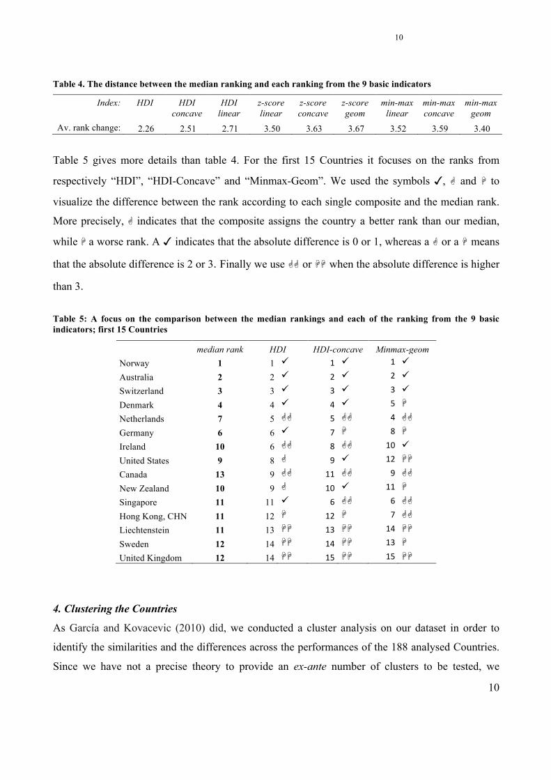
Table 4. The distance between the median ranking and each ranking from the 9 basic indicators

Index: HDI HDI HDI z-score z-score z-score min-max min-max min-max concave linear linear concave geom linear concave geom Av. rank change: 2.26 2.51 2.71 3.50 3.63 3.67 3.52 3.59 3.40

Table 5 gives more details than table 4. For the first 15 Countries it focuses on the ranks from

respectively “HDI”, “HDI-Concave” and “Minmax-Geom”. We used the symbols , and to

visualize the difference between the rank according to each single composite and the median rank.

More precisely, indicates that the composite assigns the country a better rank than our median,

while a worse rank. A indicates that the absolute difference is 0 or 1, whereas a or a means

that the absolute difference is 2 or 3 Finally we use or when the absolute difference is higher

than 3

Table 5: A focus on the comparison between the median rankings and each of the ranking from the 9 basic indicators; first 15 Countries

median rank HDI HDI-concave Minmax-geom Norway 1 1 1" 1"

Australia 2 2 2" 2"

Switzerland 3 3 3" 3"

Denmark 4 4 4" 5"

Netherlands 7 5 5" 4"

Germany 6 6 7" 8"

Ireland 10 6 8" 10"

United States 9 8 9" 12"

Canada 13 9 11" 9"

New Zealand 10 9 10" 11"

Singapore 11 11 6" 6"

Hong Kong, CHN 11 12 12" 7"

Liechtenstein 11 13 13" 14"

Sweden 12 14 14" 13"

United Kingdom 12 14 15" 15"

4. Clustering the Countries

As García and Kovacevic (2010) did, we conducted a cluster analysis on our dataset in order to

identify the similarities and the differences across the performances of the 188 analysed Countries.

Since we have not a precise theory to provide an ex-ante number of clusters to be tested, we

11

11

conduct a hierarchical cluster analysis as recommended by Nardo et al. (2008). We first set the

metric of the clustering (i.e., the distance between pairs of observations) as the Euclidean distance.

The analysis is then conducted on normalised data so as to avoid the “difference in scale” bias.

Consistently with our uncertainty analysis, we considered three different normalization rules, z-

score, min-max, and HDI normalizations. We also checked the outcome of the “distance from the

mean” normalization.

We adopted the Ward’s method (Ward, 1963) as linkage criterion, in order to calculate the distance

between sets of observations. According to this iterative process, at each step clusters or

observations are combined in such a way as to minimize the increase in the variance within the

groups. In order to establish the number of clusters, we used the Duda and Hart’s (1972) stopping

rule10. Such rule, is based on the ratio Je(2)/Je(1), where Je(2) is the sum of squared errors within

cluster when the data are partitioned into two clusters, and Je(1) gives the squared errors when only

one cluster is present. Larger values of the Je(2)/Je(1) ratio indicate more distinct clustering. In

Table 5, the Je(2)/Je(1) ratios are reported for the four different cluster analysis. The maximum

value that determines the number of clusters is emphasised in bold.

As expected, the standardisation rule used for the cluster analysis affects the outcome. As shown in

Table 6, according to the different standardisation, countries are grouped in five clusters (for the

min-max and the HDI rule), in four clusters (for the z-score), and in eight clusters (for the distance

from the mean).

Table 5. Values of the Je(2)/Je(1) ratio in four distinct cluster analysis

10 There exist several other "cluster validation" techniques including the choice minimizing the pseudo T-Square, the use of "internal measures" such as cohesion and separation or a mix of them also known as the “average silhouette width” (Rousseeuw, 1987). The choice of a different technique usually leads to different results in terms of number of clusters (and their composition) and may have relevant implications in the descriptive analysis of the data (Jain and Dubes, 1988). However, for the purposes of this work, the adoption of a different validation technique would not have changed its substantial results.

12

12

Table 6. Number and sizes of clusters for each cluster analysis

N. of Clusters min-max z-score HDI stand. Ratio to the mean

1 29 29 41 34 2 68 69 44 8 3 49 48 40 26 4 29 42 18 44 5 13 45 9 6 22 7 8 8 37

The dimensions of the clusters differ from one another, also when the number of clusters is the

same. For instance, according to the min-max cluster analysis we get 5 clusters composed

respectively of 29, 68, 49, 29 and 13 countries, while according to the HDI rule the 5 clusters are

composed of 41, 44, 40, 18 and 45 countries. Notice also that not only the total number of countries

by cluster, but also the composition of the single cluster changes. Overall, it is evident that a

seemingly innocuous choice, as the adoption of a particular technique of data normalization, can

strongly interfere with the outcome of the analysis of the data.

Comparing clustering resulting from different normalisations different, however, can give important

specific indications, as in this case.

A first point to emphasise is that there is a very strong correlation between clusters and their

performances in terms of HDI, particularly with the z-score and min-max standardisation. This

allows using the cluster analysis to set the cut-off points for different levels of human development

achievements.

Secondly, the min max and the z-score rules give almost identical clustering since the only relevant

difference is that min-max splits into two groups the fourth group of the z-score rule so that they

can be thought of as a subgroup of the last one. This is confirmed by considering that the last group

built with the HDI standardisation is almost the same as the last group under the z-score rule.

Finally also group 3 and 4 built with HDI standardisation are rather similar and could be re-grouped

together. As a result, we suggest keeping the same number of groups chosen in the Human

Development Reports, i.e. 4 groups, but changing the respective cut-off points.

Table 7 shows the number of countries and the cut-off points according to (i) the classification used

in the 2014 and 2015 Human Development Reports, and those implied by (ii) z-score, (iii) min-

13

13

max, and (iv) HDI normalisation rules. The cut-off points involved by the z-score and the min-max

are the more or less the same and labelled with “A”, while the ones involved by the HDI

standardisation are labelled with “B”. The resulting suggestion is to raise the cut-off points of the

Very High and High classes and to lower the cut-off of the Medium human development class.

Table 7. Number of countries in the groups under the current UNRO classification and alternatives ones suggested by our cluster analysis

Group Current HDI classification cut-offs points

z-score norm.

min-max norm.

cut-offs points “A”

HDI norm.

cut-offs points “B”

1 49 0.80 29 29 0.865 41 0.835

2 56 0.70 69 68 0.720 44 0.724

3 39 0.55 48 49 0.54 3a) 40

0.512 3b) 18

4 44 42 4a) 29

45 4b) 13

5. Conclusion

Building a composite index involves an unavoidable uncertainty, similarly and more than adding

apples and oranges. The researcher has to make many arbitrary choices, concerning relevant

indicators, normalization and aggregation rules, and weighting of the component variables. Hence

uncertainty grows with the efforts of synthesising the data, moving away who reads the composite

from the intrinsic content of the original data.

The HDI ranking, as shown in this paper and also by the paper that tackle this issue, is rather robust.

This is not surprising since only four indicators, which are also rather correlated to one another, are

used to calculate it. Still, the HDI is sensitive to small changes in its assumptions.

The difference between our analysis and previous one is epistemological11. We do not assume that

the true picture of human development exists. Therefore, we are not interested in assessing whether

HDI is biased or not. Biased with respect to what? A synthetic single picture cannot describe

multifaceted and complex objects. Some faces can be described by what Georgescu Roegen (1971)

11 For a detailed discussion of what we argue in the next few sentences see Funtowicz and Ravetz (1990) and Giampietro (2003).

14

14

named arithmomorphic notions, other by dialectical ones, e.g. quality indicators on an ordinal scale.

In any case, different units of measurement involve an unavoidably incommensurability. This,

however, does not imply that “nothing can be said”. Uncertainty analysis helps saying something,

that is, that a plausible rank range for each country exists. This is sufficiently simple to be

understood by the general public, but enough complicated to communicate that no measure of “the

true human development” can exist.

Hence, we claim that rather than the HDI rankings, a range of plausible ranks should be

communicated together with the HDI figure. This seems to us a reasonable compromise between

the need of synthesis when the analysis involves many variables and the loss of relevant

information due to composing different indicators into a single index. This would also help the

comparison across time of a single country performance, which might reveal an improvement even

if the Country does not surpass any other. As a personal comment, we find that making the results

more uncertain would also mitigate the idea that building composites is just a nice game to satisfy

our passion/obsession for competition.

A second issue that was investigated in this paper is the relationship between the HDI ranking and

possible clusters of the Countries. As for the uncertainty analysis, we used different standardisation

rules, which involves, as expected, different clustering. Nonetheless, quite a clear picture emerges.

First, there is a strict relation between levels of development and clusters. Second, the grouping of

the Countries made by the clustering analysis is different from the one currently used in the Human

Development Report. The most evident difference is that some of the Countries classified as very

highly developed are much more similar to the Countries classified as highly developed. The cluster

analysis suggests keeping the division into four groups, but changing their cut-off points.

References

Brian E., 2008, Condorcet and Borda in 1784. Misfits and Documents, Journal Electronique d´Histoire des Probabiltés et de la Statistique, 4 (1).

Cahill M. B., 2005, Is the human development index redundant? Eastern Economic Journal, 31(1), 1-5.

Casadio Tarabusi E., Palazzi P., 2004, An index for sustainable development, Banca Nazionale del Lavoro Quarterly Review, LVII, no. 229

De Muro P., Mazziotta M., Pareto A., 2011, Composite indices of development and poverty: An application to MDGs. Social indicators research 104 (1), 1-18.

Duda, R. O., and Hart P. E., 1972, "Use of the Hough transformation to detect lines and curves in pictures." Communications of the ACM 15.1, 11-15.

15

15

Floridi M., Pagni S., Falorni S., Luzzati T , 2011, An exercise in composite indicators construction: Assessing the sustainability of Italian regions, Ecological Economics, 70, 1440-1447.

Funtowicz S.O. and Ravetz J.R. , 1990, Uncertainty and Quality in Science for Policy, Kluwer Academic Publishers, the Netherlands.

Georgescu Roegen N., 1971, The entropy law and the economic process. Harvard University Press.

Giampietro M., 2003, Multi-Scale Integrated Analysis of Agroecosystems, CRC Press.

Herrero, C. R. Martinez, and Villar A., 2012, A newer human development index. Journal of Human Development and Capabilities, 13(2), 247–268.

Jain, Anil K., and Richard C. Dubes, 1988, Algorithms for clustering data. Prentice-Hall, Inc.

Klugman, J., Rodríguez, F., & Choi, H. J. , 2011, The HDI 2010: new controversies, old critiques. The Journal of Economic Inequality, 9(2), 249-288.

Kovacevic M., Aguña, C.G., 2010. Uncertainty and sensitivity analysis of the Human Development Index (No. HDRP-2010-47). Human Development Report Office (HDRO), United Nations Development Programme (UNDP).

Luzzati T., Gucciardi G., 2015, A non-simplistic approach to composite indicators and rankings: an illustration by comparing the sustainability of the EU Countries, Ecological Economics, 113, 25-38.

Melyn W. and Moesen W.W., 1991, Towards a synthetic indicator of macroeconomic performance: unequal weighting when limited information is available, Public Economic research Paper 17, CES, KU Leuven, Belgium.

Morse S., 2014, Stirring the pot: Influence of changes in methodology of the human development index on reporting by the press. Ecological Indicators, 45(October), 245–54.

Munda G., 2008, Social Multi-Criteria Evaluation for a Sustainable Economy, Springer.

Nardo M., Saisana M., Saltelli A., Tarantola S., Hoffmann A., Giovannini E., 2008, Handbook on Constructing Composite Indicators – methodology and user guide. OECD publishing

Paruolo P., Saisana M., Saltelli A., 2013, Ratings and rankings: Voodoo or Science?, Journal of the Royal Statistical Society A, 176 (2), 1-26.

Rousseeuw P. J., 1987,"Silhouettes: a graphical aid to the interpretation and validation of cluster analysis." Journal of computational and applied mathematics 20, 53-65.

Saisana M., Munda G., 2008, Knowledge Economy: Measures and drivers. EUR Reports 23486, EN, European Commission, JRC-IPSC.

Simon H. A., 1978, Rationality as process and as product of thought. The American economic review, 1-16.

Ward Jr, Joe H. 1963, "Hierarchical grouping to optimize an objective function." Journal of the American statistical association 58.301, 236-244.

Zambrano, E., 2011, Functioning, capabilities and the 2010 human development index, controversies, old critiques. Human Development Research Paper 2011/11, Human Development Report Office, UNDP-HDRO. Occasional Papers.

16

16

Appendix Table A1. HDI, median rank, 10th and 90th percentile of the uncertainty analysis

17

17

Table A1. continued

18

18

Table A1. continued

19

19

Discussion Papers Collana del Dipartimento di Economia e Management, Università di Pisa Comitato scientifico: Luciano Fanti - Coordinatore responsabile Area Economica Giuseppe Conti Luciano Fanti Davide Fiaschi Paolo Scapparone Area Aziendale Mariacristina Bonti Giuseppe D'Onza Alessandro Gandolfo Elisa Giuliani Enrico Gonnella Area Matematica e Statistica Sara Biagini Laura Carosi Nicola Salvati Email della redazione: lfanti@ec.unipi.it