comparative assessment of data augmentation for semi

Comparative Assessment of Data Augmentation forSemi-Supervised Polyphonic Sound Event Detection

Lionel Delphin-Poulat, Rozenn Nicol, Cyril Plapous, Katell PeronOrange Labs - IAM

Lannion & Cesson-Sevigne, France

lionel.delphinpoulat, rozenn.nicol, cyril.plapous, [email protected]

Abstract—In the context of audio ambient intelligence systemsin Smart Buildings, polyphonic Sound Event Detection aims atdetecting, localizing and classifying any sound event recorded ina room. Today, most of models are based on Deep Learning,requiring large databases to be trained. We propose a CRNNsystem exploiting unlabeled data with semi-supervised learningbased on the “Mean teacher” method, in combination withdata augmentation to overcome the limited size of the trainingdataset and to further improve the performances. This modelwas submitted to the challenge DCASE 2019 and was rankedsecond out of 58 systems submitted. In the present study, severalconventional solutions of data augmentation are compared: timeor frequency shifting, and background noise addition. It is shownthat data augmentation with time shifting and noise addition, incombination with class-dependent median filtering, improves theperformance by 9%, leading to an event-based F1-score of 43.2%with DCASE 2019 validation set. However, these tools rely ona coarse modelling (i.e. random variation of data) of intra-classvariability observed in real life. Injecting acoustic knowledge intothe design of augmentation methods seems to be a promisingway forward, leading us to propose strategies of physics-inspiredmodelling for future work.

I. INTRODUCTION

Audio ambient intelligence has the main objective of ex-

ploiting sounds in smart buildings to infer information about

people, objects, situations and events [1]. To achieve this, tools

of sound recognition are needed to be able to detect, to localize

and to classify any sound event recorded in a room. This paper

is focused on the specific issue of polyphonic Sound Event

Detection (SED) [2], which consists in identifying both the

class and the time boundaries of audio events. The detection

is termed polyphonic in the sense that different sound events

may occur simultaneously at any given time.

Solutions for polyphonic SED have been dominated by

Deep Learning for a couple of years. Large databases are thus

required to train models. However, not only the recording, but

also the labeling of such datasets is expensive. Unlabeled data

can be used, in which case semi-supervised learning must be

implemented [3]. Another issue is that one given dataset is

usually relevant to one specific task. The consequence is that

new databases must be created as soon as the task evolves.

Data augmentation was introduced to overcome these lim-

itations. During training, datasets are artificially expanded by

inserting more or less small random variations (e.g. adding

background noise, time and/or frequency stretching, etc.) in

the available data. One alternative is to synthetize artificial

data [4], which has the potential advantage to provide more

flexibility in the variations, depending on the complexity of the

synthesis model. For instance, Scaper [5] is a Python library

allowing to synthesize soundscapes by a parametric mixing of

foreground sounds (i.e. isolated sound events) and background

sounds taken from existing datasets.

In the present paper, our objective is to compare the benefits

of 3 conventional methods of data augmentation, namely: time

or frequency shifting, and background noise addition. Section

II will give an overview of existing methods of data aug-

mentation. In Section III, the training dataset, which is taken

from DCASE challenge 2019 [2], [6], is described. Our model,

which is based on a Convolutional Recurrent Neural Network

(CRNN) in combination with a “Mean Teacher” method [7]

for semi-supervised learning, is then presented in Section IV.

The detection performance of this model in combination with

various strategies of data augmentation are analyzed in Section

V. Before concluding, standard methods of augmentation are

revisited in terms of their underlying modelling of intra-class

variability in Section VI, in the perspective of developping a

“physics-inspired” model which accounts for all the potential

causes of variations that the acoustic wave encounters during

propagation.

II. STATE OF THE ART OF DATA AUGMENTATION

A. Overall problem

The challenge of datasets used in machine learning is to

provide a representative sampling of variations which are

observed in real life, so that Neural Network models become

invariant along these variations. Ideally, supervised learning

should rely on the widest possible range of data. However,

beyond the difficulty to account for infinite variations with

only a limited number of samples, recording a large amount

of real sounds is expensive. Furthermore, labeled data are

required to achieve datasets that are exploitable for supervised

learning. In the context of SED, full labeling means to identify

both the class and the timestamp of sound events [3], [4],

which makes this operation even more costly. In this case, the

label is termed “strong”. Otherwise, i.e. if only the event class

is given, the label is termed “weak”. For all these reasons, the

size of learning databases containing real and labeled data is

inherently limited.

______________________________________________________PROCEEDING OF THE 27TH CONFERENCE OF FRUCT ASSOCIATION

ISSN 2305-7254

TABLE I. USUAL METHODS OF DATA AUGMENTATION FOR SED

Augmentation method Examples of representationdomain

background noise addition [5], [11],[12]

log Mel spectrogram or audiowaveform

time [13] (e.g. “SpecAugment”) orfrequency [14] warping

log Mel spectrogram

time or frequency masking [13]–[15](e.g. “SpecAugment”)

log Mel spectrogram

time or frequency shifting [11] log Mel spectrogram or audiowaveform

pitch shifting (equivalent to frequencyshifting) [5], [12]

log Mel spectrogram or audiowaveform

time stretching [5], [12] audio waveform

mixing of 2 sound signals from thesame class [16], [17], or from differentclasses (e.g. “mixup”) [18]–[20],sometimes with randomly chosentimings [16], [17]

audio waveform

random frequency filtering [16], [21] log Mel spectrogram or audiowaveform

B. Solutions

To overcome the limitation of learning datasets, several

solutions have been proposed. Supplementing labeled data

with unlabeled data was introduced at the challenge DCASE

2018 (Task 4) [3]. However, using unlabeled data requires the

development of solutions based on semi-supervised learning.

Existing datasets can be artificially augmented by adding

subtly modified (i.e. randomly varied) copies of data, which

is referred to as data augmentation. The main methods of data

augmentation implemented to date in the field of audio pro-

cessing (e.g. speech, sound recognition or music annotation)

are listed in Table I. General description is given, but each spe-

cific implementation may differ in some aspects (modification

applied to the raw data or after feature extraction, fixed or

frame-varying parameters). Besides, it should be noticed that

the method of data augmentation may depend more or less

strongly on the SED model, particularly on its architecture.

A third solution to boost the size of learning datasets

consists in artificially creating synthetic data by appropriate

methods of sound synthesis. One advantage is that strong

labels are automatically derived from the synthesis parameters.

The complexity range of the underlying synthesis models is

wide. One simple way is a parametric mixing of audio clips

taken from databases, possibly including sound deformations

such as those previously described for data augmentation (cf.

Table I) [5]. This method was used for Task 4 of DCASE

2019 challenge. A synthetic dataset was generated with the

Scaper library [5], by randomly superimposing foreground

sound events (from the Freesound Dataset [8]) to background

soundscapes (from the SINS dataset [9]), in a way similar to

the morphological model introduced in [10] and which rely

on perception and cognition processes revealed by Auditory

TABLE II. PARAMETERS OF AUGMENTATION METHODS

Method Time shifting(frames)

Frequencyshifting(bands)

Noiseaddition(dB)

Parameter frame shift band shift SNR

Range [-270, 270] [-8, 8] [15, 40]

Probability law normal normal uniform

Mean 0 0 N.A.

Standard deviation 90 8/3 N.A.

Scene Analysis (ASA). This method of creating synthetic data

is very close to data augmentation, and could be considered

as an improved or generalized way of augmenting datasets.

Besides, Scaper is presented as a library for both sound

synthesis and data augmentation.

C. Experiments

A comprehensive comparison of augmentation methods is

beyond the scope of the present study. To give a first insight,

we have selected three strategies [11] of data augmentation:

• Time shifting: The matrix representing the Mel spectro-

gram of the audio sample is translated along its frame

axis. It should be noticed that the translation is circular,

i.e. in the case of a forward shift, the last frames are

moved to the beginning, whereas, in the case of a

backward shift, the early frames are moved to the end.

In addition, labels must be modified accordingly, so that

the new time boundaries of sound events reflect the time

translation. The motivation for time shifting is to enhance

the invariance of the SED model with respect to the

occurrence times of events.

• Frequency shifting: The matrix of the Mel spectrogram

is translated along its frequency axis. In the case of an

upward shift of kt bands (kt ∈ N), the values of the first

kt bins are replaced by the value of the bin k = kt + 1.

In the case of a downward shift of kt bands, the values

of the last kt bins are replaced by the value of the bin

k = K − kt, where K is the number of bands. It can be

remarked that frequency shifting of log Mel spectrograms

is an approximation of pitch shifting [5]. In a similar vein,

the purpose of time or frequency masking [15] is close

to that of the regularization method called “Dropout”.

• Noise addition: A random value, with respect to a given

Signal-to-Noise Ratio (SNR), is added to each value of

the Mel spectrogram.

In addition, the benefit of data augmentation vs addition of

synthetic data is evaluated. To generate new training data, each

audio clip is transformed in the log Mel domain by applying

one of these methods with a set of parameters randomly

selected according to a probability distribution as defined in

Table II. One fixed parameter value is applied per audio clip.

The whole training dataset (i.e. both real and synthetic data)


---------------------------------------------------------------------------- 47 ----------------------------------------------------------------------------

TABLE III. TESTED CONFIGURATIONS OF THE LEARNING DATASET (EACH CONFIGURATION IS REFERRED TO AS “LX”, WHERE X IS THE INDEX OF THE

LEARNING CONFIGURATION)

Option L1 L2 L3 L4 L5 L6 L7 L8 L9

Synthetic data x x x x x x x x

Time shifting x x x x

Frequency shifting x x x x

Noise addition x x x x

is used in the augmentation process. The performance of the

same model of SED with these different configurations of the

learning dataset, as illustrated in Table III, are then assessed

to highlight the relative benefits of each strategy.

III. DATASET

A. DCASE challenge 2019

For this study, we used the dataset proposed for the DCASE

challenge 2019 (Task 4) [4]. It contains 10-sec audio clips

(original sampling frequency: 44,100 Hz). Each clip contains

at least one sound event belonging to one of the 10 fol-

lowing classes: Speech, Dog, Cat, Alarm/bell/ringing, Dishes,

Frying, Blender, Running water, Vacuum cleaner, Electric

shaver/toothbrush. The training set is composed of 3 subsets:

• Weakly labeled and unbalanced subset: 1578 clips, real

recordings (taken from the “AudioSet” database [22])

• Unlabeled and unbalanced in domain subset: 14412 clips,

real recordings [22],

• Strongly labeled and unbalanced subset: 2045 clips, syn-

thetic data generated by the “Scaper” software [5]

The validation set consists of real recordings (1168 clips

containing a total of 4093 events) with strong labels. The

evaluation set comprises both real recordings (1013 clips) and

synthetic data (12139 clips, with varying properties of SNR,

audio degradation, onset time of sound events, etc.). However,

the performance presented in the following are based on the

validation set of DCASE challenge 2019.

B. Audio preprocessing

The dataset contains some files which consist only of

numerical zeros, and which were therefore removed. It was

also observed that the DC level is strong in some cases, which

is useless. Consequently, the DC component was suppressed.

If necessary, the audio clip was down-mixed to a monophonic

signal, which is obtained as the average of all the channels.

Then the audio clips were down-sampled at 22,050 Hz, since

high-frequencies are assumed to be irrelevant for SED, and

the log Mel spectrogram was extracted. To do this, the size

of the analysis window was 2048 samples (i.e. approximately

92.9 ms), with a hop length of 365 samples (i.e. approximately

16.6 ms). The number of Mels was fixed at 128. Finally, the

Mel spectrogram, S(i, n, k) (where i, n, and k refer to the

audio sample index, the frame index, and the frequency bin,

respectively), was standardized. For this, a mean, Smean(k),and standard deviation, Ssd(k), were computed for each fre-

quency bin over all the training set (i.e. over all the frames

and samples), leading to a standardization specific to each bin:

Sstd(i, n, k) =S(i, n, k)− Smean(k)

Ssd(k)

where Sstd is the standardized Mel spectrogram.

IV. TRAINING AND MODEL

A. Semi-supervised learning: “Mean Teacher” method

Since the training set contains unlabeled data, semi-

supervised learning is necessary. Our training strategy is

inspired by the solution presented in [23]. It is based on

the“Mean Teacher” method [7], [23], which makes two vari-

ants of the model, the teacher and the student, work together.

The student is learning in a way similar to that of supervised

learning, except that the labels of unlabeled data are provided

by the teacher. At the same time, the teacher model is

adjusted at each training step to replicate the student model.

The process is governed by 2 losses: the classification cost

and the consistency cost, the latter being added to measure

the expected distance between the prediction of the student

and that of the teacher model. To improve the reliability of

the labels generated by the teacher, a first solution consists

in adding noise to the input data of the teacher (Gaussian

noise, with 22-dB SNR). Further improvement is achieved

by forming the prediction of each example from not only

the prediction provided by the current version of the model,

but also from the predictions given for the same example by

earlier versions of the model. The result is computed as the

Exponential Moving Average (EMA) of all the predictions (the

coefficient of the moving averaging is set to 0.999). However,

it was shown that the teacher accuracy is increased if the model

weights, instead of the predictions, are averaged, leading to the

“Mean Teacher” method [7]. Eventually, the inference model

is the student model, the teacher model being used only to

help the student’s learning.

Our training procedure differs in one aspect from the

original “Mean Teacher” method. We have remarked that the

teacher has consistently better performance than the student,

leading us to select the teacher model as the inference model.

The teacher could be seen as an ensemble version of the

students, with the difference that EMA is applied instead of

averaging the students. Thus it can also be considered as a

regularization approach, which could explain the consistently

better results achieved by the teacher throughout our experi-

ments.

B. CRNN architecture

The architecture of our model is derived from the baseline

model of the DCASE challenge 2019 (Task 4) [4]. It is based

on a CRNN, composed of 7 convolutional layers (filter size

[3x3], time and frequency padding: [1,1], time and frequency

stride: [1,1], 50% dropout, Gated Linear Units GLU, see

Table IV for a detailed description of the different layers) and


---------------------------------------------------------------------------- 48 ----------------------------------------------------------------------------

TABLE IV. PROPERTIES OF THE CONVOLUTIONAL LAYERS

Layer 1 2 3 4 5 6 7

number of filters 16 32 64 128 128 128 128

time max pooling 2 2 1 1 1 1 1

frequency max pooling 2 2 2 2 2 2 2

TABLE V. MAXIMUM NUMBER OF EPOCHS

Training part Number of clips Maximum numberof batches

weakly labeled data 1578 � 15786

� = 263

unlabeled data 14412 � 1441212

� = 1201

strongly labeled data 2045 � 20456

� = 340

2 recurrent layers (bidirectional Gated Recurrent Units GRUfor each layer with 128 features for the hidden layer in each

direction, 50% dropout, sigmoid activation and softmax on the

output layer).

We kept the batch size and composition that was provided in

the baseline system, i.e. the number of clips in one batch is 24.

When strongly labeled data are used, the batch composition is

the following:

• 6 weakly labeled clips

• 12 unlabeled clips

• 6 strongly labeled clips

When strongly labeled data are not used, the batch is made

up of:

• 6 weakly labeled clips

• 18 unlabeled clips

Each clip appears at most once during one epoch. Then we

can deduce the maximum number of batches for each training

part as depicted in Table V and the number of batches Be

in one epoch is equal to the smallest of these numbers, i.e.

Be = 263.

The training process includes a ramp-up strategy. When

training begins, the predictions provided by the teacher model

are poor. Thus, the weight of the consistency cost in the total

loss is small at the beginning and is increased during training

when the labels provided by the master become more and

more reliable. Similarly, when training starts, the parameter

updates in the gradient descent should be cautious, i.e. with a

small learning rate. As training makes progress, the learning

rate can be increased. More precisely, let b be the batch count

across epochs, and let r(b) be a ramp-up function defined in

equation 1:

r(b) =

⎧⎨⎩exp

(−5

(1− b

bmax

)2), if b ≤ bmax

1, otherwise

(1)

TABLE VI. DURATION OF SOUND EVENTS FOR EACH CLASS

Class Occurrences Mean in s Median in s

Alarm/bell/ringing 755 1.07 0.38

Blender 540 2.58 1.62

Cat 547 1.07 0.88

Dishes 814 0.58 0.37

Dog 516 0.98 0.48

Electric shaver/toothbrush 230 4.52 4.07

Frying 137 5.17 5.13

Running water 157 3.91 3.60

Speech 2132 1.16 0.89

Vacuum cleaner 204 5.29 5.30

This function starts from a very small value and reaches 1after bmax = Be × emax batches, where emax is set to 50epochs. In the baseline system, r(b) was only used to weight

the consistency cost. In our training set-up, it was also used

to update the learning rate μ(b) as follows:

μ(b) = μmaxr(b)

where μmax = 0.001. The system is thus trained for 400

epochs. The optimization algorithm is Adam.

C. Postprocessing by class-dependent median filtering

The model outputs an estimated class for each frame. This

information can be used to determine the onset and offset

times of events for each audio clip. However, due to the

incertainty of event classification, the detection may suffer

from discontinuities. For instance, the sound of the vacuum

cleaner usually lasts for at least several seconds. But, it

happens that it is detected in one frame, but is not detected in

the next one, and yet is detected again in the following frames.

It is highly unlikely that it would disappear for just one frame.

To avoid such spurious detection, median filtering is used to

postprocess the frame-by-frame outputs. A median filter is

a nonlinear filter which is especially efficient for removing

impulse noise. In the context of SED, the neural network

provides, frame by frame, a detection probability of all event

classes. An event activity indicator is computed by applying

a threshold to the probability: the indicator is set to 1 if the

probability is greater than 0.5 and to 0 otherwise. The detection

indicator associated to each class is then smoothed along time

axis by a median filter, which replaces the value centered in

a given window with the median of all the values contained

in this window. It has been shown that it is advantageous to

vary the length of the sliding median window as a function of

the event class, more exactly as a function of the duration of

the associated sound event [15], [25], [26].

The mean and median event durations were computed for

each class (see Table VI) over the synthetic training subset,

allowing us to define 3 main categories of sound events:


---------------------------------------------------------------------------- 49 ----------------------------------------------------------------------------

Fig. 1. Event-based and segment-based F1-score of the 10 models

• Impulsive sounds: “Alarm/bell/ringing”, “Dishes” and

“Dog”, the median duration of which is less than 0.5 s.

• Intermediate sounds: “Blender”, “Cat” and “Speech”, the

median duration of which is around 1 s.

• Continuous sounds: “Electric shaver/toothbrush”, “Fry-

ing”, “Running water” and “Vacuum cleaner”, the median

duration of which is greater than 3 s.

The window length of the median filter is adapted accordingly,

leading to class-dependent median filtering (CDMF):

• Impulsive sounds: 5 frames (i.e. 332 ms),

• Intermediate sounds: 13 frames (i.e. 863 ms),

• Continuous sounds: 41 frames (i.e. 2722 ms).

The window hop is set to 16.6 ms. Due to time pooling (see

Table IV), an output frame corresponds to 66.4ms (original

signal resampled at 22,050 Hz).

V. RESULTS

On the whole, 10 models are compared, among which 9

models correspond to the configurations of data augmentation

which are listed in Table III. These latter implement post-

processing by a fixed-length median filter (i.e. 9 frames, or

597 ms, see Section IV-C). The last model is based on the C9

augmentation method and includes CDMF. All the systems are

assessed in terms of the event-based (onsets: 200-ms collar,

offsets: collar defined as the greater of 200 ms and 20% of

the sound event’s length) and segment-based (1-s segments)

F1-score with class-based averaging [27]. Model performance

is computed with the validation set of DCASE challenge 2019

(Task 4). Results are illustrated in Fig. 1.

Adding synthetic data (L2 vs L1) leads to a remarkable

increase (around 10%), especially in terms of event-based

score. However, it should be kept in mind that the contribution

of synthetic data is twofold: not only do they expand the

learning dataset, but they are also strong labeled. Among the

strategies of data augmentation, time shifting (L3) and noise

addition (L6) seem to be the most advantageous (increase

of around 5% in comparison with L2). In comparison, the

contribution of frequency shifting is negligible, and sometimes

even negative (L5 vs L3, L8 vs L6, and L9 vs L7). When

combining all proposed data augmentation with CDMF, the

event-based score is improved by about 3% (L9 with CDMF

vs L9). Segment-based scores reflect similar trends, except

that the temporal granularity of these metrics (i.e. the segment

duration is much higher than a frame) obliterates the benefit

of CDMF [6]. As a result, our model obtains an event-based

F1-score of 43.2% (DCASE 2019 validation set), matching the

highest scores of the challenge [6].

Fig. 2. depicts the event-based F1-score for each class of

sound event. First, it may be remarked that the primary model

(L1) achieves very small F1-score (less than 5%) for the

classes “Cat” and “Electric shaver/toothbrush”. For these two

classes, the benefit of data augmentation is high (more than

20%). However, in the case of the class “Cat”, the main benefit

is provided by adding synthetic data (L2 vs L1), and the

increase achieved with further augmentation is minor (around

5 % at most). For some other classes, the improvement is

marginal, whichever the method of data augmentation (e.g.

“Alarm/bell/ringing”). More generally, the trends observed on

average (cf. Fig. 1) are not found for any class. In other

words, the relative contribution of each augmentation method

highly depends on the class. Nevertheless, the model which

combines all strategies of data augmentation with CDMF

(i.e. L9 wi CDMF) stands out with the highest F1-score

in half of the classes (namely: “Dishes”, “Dog”, “Electric

shaver/toothbrush”, “Frying”, “Vacuum cleaner”). In the case

of the class “Electric shaver/toothbrush”, the performance is

increased by around 56% in comparison with the model L1.

For the other classes (i.e. “Alarm/bell/ringing”, “Blender”,

“Cat”, “Running water”, “Speech”), the decrease in perfor-

mance observed when using a CDMF raises the question of

whether the adaptation of the median filter to these categories

of sound events could be improved, yet with the risk of

overfitting. Indeed, it should be noticed that, when evaluated

with audio clips of the Vimeo dataset (composed of real

recordings) [4], our model achieves the highest score, differing

significantly from the other systems submitted to the challenge.

This result suggests that it offers a good compromise between

adaptation and generalization.

VI. DISCUSSION: DATA AUGMENTATION INTO QUESTION

The methods of data augmentation that have been tested in

the foregoing are a simplistic, yet effective way of modelling

the intra-class variability of real-life sound scenes. Indeed, they

are mainly based on signal transformations (either in the time

domain, or in the frequency domain, but rarely in the time-

frequency domain), whose parameters are randomly selected

in arbitrarly defined sets. In other words, the link between

these methods and the physical phenomena which are causing

these variabilities is generally weak.

A. Acoustics and intra-class variability of sound scenes

In the domain of sound recognition, data are acoustic signals

which represent acoustic waves emitted by sound sources


---------------------------------------------------------------------------- 50 ----------------------------------------------------------------------------

Fig. 2. Event-based F1-score of the 10 models for the 10 sound event classes

and recorded by one or several microphones in a given

environment. Therefore, each observed realization of a sound

scene is governed by the following components:

• The primary sound source, from which the acoustic wave

orginates: Variations in the sound production may occur,

modifying the temporal and/or spectral content, as well

as the sound level.

• The acoustic environment: The walls of the room or

any object interact with the acoustic wave, resulting

in delayed and spectrally modified copies of the direct

sound, which are superimposed on the latter. These

phenomena are usually modelled by the impulse (or

frequency) response of the room, which depends on both

the position of the source and the receiver.

• Interfering sources: Generally the target source is not the

only sound source present in the environment. In this

case, other sources are likely to interfere with the source

of interest, leading to a decrease of the Signal-to-Noise

Ratio (SNR) if the sound level of the interferer is low,

or to time and/or frequency masking if it is close to or

higher than the level of the target source.

• The recording setup: In this final stage, the microphone

arrangement (i.e. one single microphone or a microphone

array), the frequency and directional response of each

transducer, their internal noise and their sensitivity affect

the recorded signals.


---------------------------------------------------------------------------- 51 ----------------------------------------------------------------------------

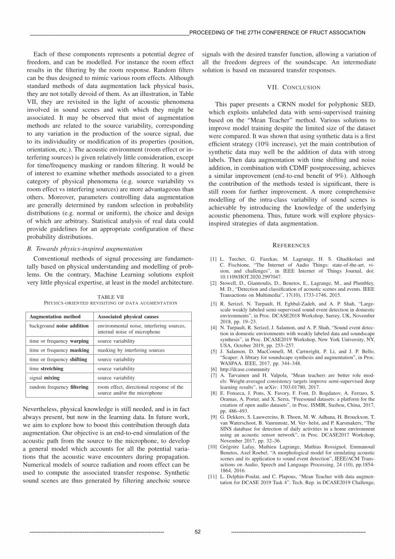
Each of these components represents a potential degree of

freedom, and can be modelled. For instance the room effect

results in the filtering by the room response. Random filters

can be thus designed to mimic various room effects. Although

standard methods of data augmentation lack physical basis,

they are not totally devoid of them. As an illustration, in Table

VII, they are revisited in the light of acoustic phenomena

involved in sound scenes and with which they might be

associated. It may be observed that most of augmentation

methods are related to the source variability, corresponding

to any variation in the production of the source signal, due

to its individuality or modification of its properties (position,

orientation, etc.). The acoustic environment (room effect or in-

terfering sources) is given relatively little consideration, except

for time/frequency masking or random filtering. It would be

of interest to examine whether methods associated to a given

category of physical phenomena (e.g. source variability vs

room effect vs interfering sources) are more advantageous than

others. Moreover, parameters controlling data augmentation

are generally determined by random selection in probability

distributions (e.g. normal or uniform), the choice and design

of which are arbitrary. Statistical analysis of real data could

provide guidelines for an appropriate configuration of these

probability distributions.

B. Towards physics-inspired augmentation

Conventional methods of signal processing are fundamen-

tally based on physical understanding and modelling of prob-

lems. On the contrary, Machine Learning solutions exploit

very little physical expertise, at least in the model architecture.

TABLE VIIPHYSICS-ORIENTED REVISITING OF DATA AUGMENTATION

Augmentation method Associated physical causes

background noise addition environmental noise, interfering sources,internal noise of microphone

time or frequency warping source variability

time or frequency masking masking by interfering sources

time or frequency shifting source variability

time stretching source variability

signal mixing source variability

random frequency filtering room effect, directional response of thesource and/or the microphone

Nevertheless, physical knowledge is still needed, and is in fact always present, but now in the learning data. In future work, we aim to explore how to boost this contribution through data augmentation. Our objective is an end-to-end simulation of the acoustic path from the source to the microphone, to develop a general model which accounts for all the potential varia-

tions that the acoustic wave encounters during propagation. Numerical models of source radiation and room effect can be used to compute the associated transfer response. Synthetic sound scenes are thus generated by filtering anechoic source

VII. CONCLUSION

This paper presents a CRNN model for polyphonic SED,

which exploits unlabeled data with semi-supervised training

based on the “Mean Teacher” method. Various solutions to

improve model training despite the limited size of the dataset

were compared. It was shown that using synthetic data is a first

efficient strategy (10% increase), yet the main contribution of

synthetic data may well be the addition of data with strong

labels. Then data augmentation with time shifting and noise

addition, in combination with CDMF postprocessing, achieves

a similar improvement (end-to-end benefit of 9%). Although

the contribution of the methods tested is significant, there is

still room for further improvement. A more comprehensive

modelling of the intra-class variability of sound scenes is

achievable by introducing the knowledge of the underlying

acoustic phenomena. Thus, future work will explore physics-

inspired strategies of data augmentation.

REFERENCES

[1] L. Turchet, G. Fazekas, M. Lagrange, H. S. Ghadikolaei andC. Fischione, “The Internet of Audio Things: state-of-the-art, vi-sion, and challenges”, in IEEE Internet of Things Journal, doi:10.1109/JIOT.2020.2997047.

[2] Stowell, D., Giannoulis, D., Benetos, E., Lagrange, M., and Plumbley,M. D., “Detection and classification of acoustic scenes and events. IEEETransactions on Multimedia”, 17(10), 1733-1746, 2015.

signals with the desired transfer function, allowing a variation of all the freedom degrees of the soundscape. An intermediate solution is based on measured transfer responses.

[3] R. Serizel, N. Turpault, H. Eghbal-Zadeh, and A. P. Shah, “Large-scale weakly labeled semi-supervised sound event detection in domesticenvironments”, in Proc. DCASE2018 Workshop, Surrey, UK, November2018, pp. 19–23.

[4] N. Turpault, R. Serizel, J. Salamon, and A. P. Shah, “Sound event detec-tion in domestic environments with weakly labeled data and soundscapesynthesis”, in Proc. DCASE2019 Workshop, New York University, NY,USA, October 2019, pp. 253–257.

[5] J. Salamon, D. MacConnell, M. Cartwright, P. Li, and J. P. Bello,“Scaper: A library for soundscape synthesis and augmentation”, in Proc.WASPAA. IEEE, 2017, pp. 344–348.

[6] http://dcase.community[7] A. Tarvainen and H. Valpola, “Mean teachers are better role mod-

els: Weight-averaged consistency targets improve semi-supervised deeplearning results”, in arXiv: 1703.01780, 2017.

[8] E. Fonseca, J. Pons, X. Favory, F. Font, D. Bogdanov, A. Ferraro, S.Oramas, A. Porter, and X. Serra, “Freesound datasets: a platform for thecreation of open audio datasets”, in Proc. ISMIR, Suzhou, China, 2017,pp. 486–493.

[9] G. Dekkers, S. Lauwereins, B. Thoen, M. W. Adhana, H. Brouckxon, T.van Waterschoot, B. Vanrumste, M. Ver- helst, and P. Karsmakers, “TheSINS database for detection of daily activities in a home environmentusing an acoustic sensor network”, in Proc. DCASE2017 Workshop,November 2017, pp. 32–36.

[10] Gregoire Lafay, Mathieu Lagrange, Mathias Rossignol, EmmanouilBenetos, Axel Roebel, “A morphological model for simulating acousticscenes and its application to sound event detection”, IEEE/ACM Trans-actions on Audio, Speech and Language Processing, 24 (10), pp.1854-1864, 2016.

[11] L. Delphin-Poulat, and C. Plapous, “Mean Teacher with data augmen-tation for DCASE 2019 Task 4”, Tech. Rep. in DCASE2019 Challenge,


---------------------------------------------------------------------------- 52 ----------------------------------------------------------------------------

Orange Labs, July 2019.[12] J. Salamon and J. P. Bello, “Deep convolutional neural networks and data

augmentation for environmental sound classification”, in IEEE SignalProcessing Letters, vol. 24, no. 3, pp. 279-283, March 2017.

[13] D. S. Park, W. Chan, Y. Zhang, C.-C. Chiu, B. Zoph, E. D. Cubuk,and Q. V. Le, “SpecAugment: A simple data augmentation methodfor automatic speech recognition”, in Proc. INTERSPEECH 2019, pp.2613–2617, arXiv:1904.08779.

[24] S. Laine and T. Aila, “Temporal Ensembling for Semi-SupervisedLearning”, in ICLR 2017, arXiv: 1610.02242, 2017.

[14] J. Ebbers, and R. Hab-Umbach, “Convolutional recurrent neural networkand data augmentation for audio tagging with noisy labels and minimalsupervision”, in Proc. DCASE2019 Workshop, New York University,NY, USA, October 2019, pp. 64–68.

[15] W. Lim, “SpecAugment for sound event detection in domestic environ-ments using ensemble of convolutional recurrent neural networks”, inProc. DCASE2019 Workshop, New York University, NY, USA, October2019, pp. 129–133.

[16] N. Takahashi, M. Gygli, B. Pfister, and L. Van Gool, “Deep con-volutional neural networks and data augmentation for acoustic eventrecognition”, in Proc. INTERSPEECH 2016, arXiv:1604.07160.

[17] T. Inoue, P. Vinayavekhin, S. Wang, D. Wood, A. Munawar, B. J. Ko,N. Greco, and R. Tachibana, Ryuki, “Shuffling and mixing data aug-mentation for environmental sound classification”, in Proc. DCASE2019Workshop, New York University, NY, USA, October 2019, pp. 109–113.

[18] Y. Tokozume, Y. Ushiku, and T. Harada, “Learning from between-class examples for deep sound recognition”, in Proc. ICLR 2018,arXiv:1711.10282.

[19] H. Zhang, M. Cisse, Y. N. Dauphin, and D. Lopez-Paz, “Mixup: Beyondempirical risk minimization”, in Proc. ICLR 2018, arXiv:1710.09412.

[20] P. Pratik, W. J. Jee, S. Nagisetty, R. Mars, and C. Lim, Chongsoon,“Sound event localization and detection using CRNN architecture withmixup for model generalization”, in Proc. DCASE2019 Workshop, NewYork University, NY, USA, October 2019, pp. 99–203.

[21] L. Delphin-Poulat, C. Plapous, and R. Nicol, “GCNN for classificationof domestic activities”, Tech. Rep. in DCASE2018 Challenge, OrangeLabs, July 2018.

[22] J. F. Gemmeke, D. P. W. Ellis, D. Freedman, A. Jansen, W. Lawrence,R. C. Moore, M. Plakal, and M. Ritter, “Audio set: An ontology andhuman-labeled dataset for audio events”, in Proc. ICASSP, 2017.

[23] L. JiaKai, “Mean teacher convolution system for DCASE 2018 Task 4”,Tech. Rep. in DCASE2018 Challenge, PFU Shanghai, July 2018.

[25] W. Lim, S. Suh, and Y. Jeong, “Weakly labeled semi-supervised soundevent detection using CRNN with inception module”, Tech. Rep. inDCASE2018 Challenge, Electronics and Telecommunications ResearchInstitute, Korea, July 2018.

[26] H. Dinkel, and K. Yu, “Duration robust weakly supervised sound eventdetection”, in Proc. ICASSP, 2020, arXiv:1904.03841v3.

[27] A. Mesaros, T. Heittola and T. Virtanen, “Metrics for polyphonic soundevent detection”, in Appl. Sci, 6, 162, 2016.


---------------------------------------------------------------------------- 53 ----------------------------------------------------------------------------

comparative assessment of data augmentation for semi

Documents