comparative study of backpropagation algorithms in

Science Journal of Applied Mathematics and Statistics 2016; 4(3): 88-96 http://www.sciencepublishinggroup.com/j/sjams doi: 10.11648/j.sjams.20160403.11 ISSN: 2376-9491 (Print); ISSN: 2376-9513 (Online)

Comparative Study of Backpropagation Algorithms in Forecasting Volatility of Crude Oil Price in Nigeria

S. Suleiman1, S. U. Gulumbe

1, B. K. Asare

1, M. Abubakar

2

1Department of Mathematics, Usmanu Danfodiyo University, Sokoto, Nigeria 2Department of Economics, Usmanu Danfodiyo University, Sokoto, Nigeria

Email address: [email protected] (S. Suleiman), [email protected] (S. Suleiman)

To cite this article: S. Suleiman, S. U. Gulumbe, B. K. Asare, M. Abubakar. Comparative Study of Backpropagation Algorithms in Forecasting Volatility of

Crude Oil Price in Nigeria. Science Journal of Applied Mathematics and Statistics. Vol. 4, No. 3, 2016, pp. 88-96.

doi: 10.11648/j.sjams.20160403.11

Received: April 5, 2016; Accepted: April 19, 2016; Published: May 7, 2016

Abstract: This paper explores the application of artificial neural network in volatility forecasting. A recurrent neural

network has been integrated in to GARCH model to form the hybrid model called GARCH-Neural model. The emphasis of the

research is to investigate the performance of the variants of Backpropagation algorithms in training the proposed GARCH-

neural model. In the first place, EGARCH (3, 3) was identified in this paper most preferred model describing crude oil price

volatility in Nigeria. Similarly, Levenberg-Marquardt (LM) training algorithms were found to be fastest in convergence and

also provide most accurate predictions of the volatility when to other training techniques.

Keywords: GARH Models, Recurrent Neural Networks, Backpropagation Algorithms and Forecasting

1. Introduction

Crude oil is considered to be an important export

commodity in Nigeria because of its contribution to the

economy of the country. It was first discovered in 1958 and

first produced well in 1956. Before that time, the country

mainly depends on the exports of the agricultural

commodities that comprised groundnuts, cocoa beans, palm

oil, cotton and rubber. Palm oil was the leading export from

1946-1958, followed by cocoa beans while groundnut/oil

ranked third. From a production level of 1.9 million barrels

per day in 1958, crude oil exports rose to 2.35 million barrels

per day in the early 2000s. However, it had fluctuated

between 2.35 and 2.40 million barrels per day between 2011

and 2015 which was far below the OPEC quota due to the

socio-political instability in the oil-producing areas of the

country. In terms of its contribution to total revenue, receipts

from oil that constituted 26.3 per cent of the federally

collected-revenue in 1970, rose to 82.1 per cent in 1974 and

83.0 per cent in 2008 largely on account of a rise in crude oil

prices at the international market.

Over the last two years, global oil prices have been dropping

and bearing in mind that Nigeria is an import dependent

economy, this development is worrisome. Our reviews of the

current oil exports also reveal a southward trend due to

significant oil theft and lower global demands. Indeed, NNPC

(Nigerian National Petroleum Corporation) puts total value of

revenue loss due to oil theft at $11bn in 2013.

More importantly, crude oil for the last three decades has

been the major source of revenue, energy and the foreign

exchange for the Nigerian economy. In 2000 oil and gas

export earnings accounted for about 98% and about 83% of

federal government revenue. [1].

The term volatility has been given different definitions by

different scholars across disciplines. In relation to crude oil

price, volatility is the variation in the worth of a variable,

especially price [2]. Volatility is the measure of the tendency

of oil price to rise or fall sharply within a period of time, such

as a day, a month or a year [3]. [4] Defines volatility as the

standard deviation in a given period. She notes that volatility

has a negative and significant impact on economic growth

instantly, while the impact of oil price changes delays until

after a year. She concludes by saying that ―it is

volatility/change in crude oil prices rather than oil price level

that has a significant influence on economic growth. In a

nutshell, volatility is a measurement of the fluctuations (i.e

rise and fall) of the price of commodity for example oil price

89 S. Suleiman et al.: Comparative Study of Backpropagation Algorithms in Forecasting Volatility of Crude Oil Price in Nigeria

over a period of time.

Artificial neural networks (ANNs) have been known to

have the capability to learn the complex approximate

relationships between the inputs and the outputs of the

system and are not restricted by the size and complexity of

the system [5]. The ANNs learn these approximate

relationships on the basis of actual inputs and outputs.

Therefore, they are generally more accurate as compared to

the relationships based on assumptions. ANNs have been

used for volatility forecasting in several papers for example

[6-10]. Despite their popularity in applications to financial

variables, ANNs have not been utilized very well in Nigerian

financial market. Similarly, multi-layer feedforward Artificial

Neural Networks using Backpropagation algorithms for

training have been used in several literatures for example

[11-14]. Since the Backpropagation algorithm has been

successfully applied to train neural networks, this work aims

to investigate the training performance of the some variants

of the back propagation algorithm in training the proposed

model for forecasting volatility.

2. Volatility Models

Let �� be stock price at time �. Then

�� = 100( �� − �� ) (1)

denotes the continuously compounded daily returns of the

underlying assets at time �. The most widely used model for estimating volatility is

ARCH (Auto Regressive Conditional Heteroscedasticity) model developed by [15] as also contained in [33]. Since the development of the original ARCH model, a lot of research has been carried out on extensions of this model among which

GARCH [16] and is defined as �� = �� + �� , �� = �� , and

�� = � + ∑ ��

�� + ∑ ��

�� (2)

�, ��, �� are non-negative parameters to be estimated, �� is

an independently and identically distributed (i.i.d.) random

variables with zero mean and unit variance and �� is a serially uncorrelated sequence with zero mean and the conditional

variance of �� which may be nonstationary, the GARCH model reduces the number of parameters necessary when information in the lag (s) of the conditional variance in

addition to the lagged �� terms were considered, but was

not able to account for asymmetric behavior of the returns.

Because of this weakness of GARCH model, a number of

extensions of the GARCH (p, q) model have been developed

to explicitly account for the skewness or asymmetry. The

popular models of asymmetric volatility includes, the

exponential GARCH (EGARCH) model, [17] GJR-GARCH

model, asymmetric power ARCH (APARCH).

The GJR-GARCH (p, q) model was introduced by [9] to

allow for allows asymmetric effects. The model is given as:

�� = � + ∑ ��

�� + ∑ ��

�� + ∑ !�� !�"

!�� #� ! (3)

Where #� (a dummy variable) =1 if �� < 0 & 0 otherwise.

In the GJR-GARCH model, good news �� > 0 and bad

news, �� < 0, have differential effects on the conditional

variance; good news has an impact of �� while bad news has

an impact of �� + < 0 . If � > 0, bad news increases

volatility, and there is a leverage effect for the '�ℎ −order. if

≠ 0, the news impact is asymmetric [17]. The exponential GARCH (EGARCH) model advanced by [18] is the earliest extension of the GARCH model that incorporates asymmetric effects in returns from speculative prices. The EGARCH model is defined as follows:

*+�� = � + ∑ �� ,-./01./0

− 2(-./01./0

),�� + ∑ ��*+��

�� + ∑ !(-./3

1./3)"

!�� (4)

Where �, �� , �� and ! are constant parameters. The

EGARCH (p, q) model, unlike the GARCH (p, q) model, indicates that the conditional variance is an exponential function, thereby removing the need for restrictions on the parameters to ensure positive conditional variance. The asymmetric effect of past shocks is captured by the γ coefficient, which is usually negative, that is, cetteris paribus positive shocks generate less volatility than negative shocks [19]. The leverage effect can be tested if γ < 0. If γ ≠ 0, the news impact is asymmetric.

The asymmetry power ARCH (APARCH) model of [20]

also allows for asymmetric effects of shocks on the

conditional volatility. Unlike other GARCH models, in the

APARCH model, the power parameter of the standard

deviation can be estimated rather than imposed, and the

optional γ parameters are added to capture asymmetry of up

to order r. The APARCH (p, q) model is given as:

��4 = � + ∑ ��(|�� | − �� )4 +�� ∑ ��*+��

4�� (5)

where δ >0, i γ ≤1 for i =1, …, r, γi = 0 for all I > r, and r ≤ p

If γ ≠ 0, the news impact is asymmetric.

The introduction and estimation of the power term in the

APARCH model is an attempt to account for the true

distribution underlying volatility [33]. The idea behind the

introduction of a power term arose from the fact that, The

assumption of normality in modeling financial data, which

restricts d to either 1 or 2, is often unrealistic due to

significant skewness and kurtosis [19]. Allowing d to take the

form of a free parameter to be estimated removes this

arbitrary restriction.

3. Recurrent Neural Networks

Neural networks can be classified into static and dynamic

categories [21]. Static networks have no feedback elements

and contain no delays; the output is calculated directly from

the input through feed forward connections. In dynamic

networks, the output depends not only on the current input to

the network, but also on the current or previous inputs,

outputs, or states of the network. These dynamic networks

Science Journal of Applied Mathematics and Statistics 2016; 4(3): 88-96 90

may be recurrent networks with feedback connections or feed

forward networks with imbedded tapped delay lines (or a

hybrid of the two). For static networks, the standard back

propagation algorithm [22] can be used to compute the

gradient of the error function with respect to the network

weights, which is needed for gradient-based training

algorithms. For dynamic networks, a more complex dynamic

gradient calculation must be performed. Although they can

be trained using the same gradient-based algorithms that are

used for static networks, the performance of the algorithms

on dynamic network can be quite different and the gradient

must be computed in a more complex way [23]

Dynamic networks are generally more powerful than static

networks (although somewhat more difficult to train).

Because dynamic networks have memory, they can be trained

to learn sequential or time-varying patterns. This has

applications in such disparate areas as prediction in financial

markets [24], phase detection in power systems [25] and

many more dynamic network applications in [26].

The Non-linear Auto-Regressive with Exogenous (NARX)

inputs is a recurrent dynamic network, with feedback

connections enclosing several layers of the network. The

NARX model is based on the linear ARX model, which is

commonly used in time-series modeling.

The defining equation for the NARX model is as follow:

�(�) = 6(�(� − 1�, �� 2� … , �� , 9�� 1�, 9�� 2�, … , 9�� (6)

Where the next value of the dependent output signal �� is regressed on the previous values of the output signal and previous values of an independent (exogenous) input signals.

A diagram showing the implementation of the NARX model using a feed forward neural network to approximate the

function 6 in (6) is given in figure 1

Fig. 1. Implementation of NARX model.

Fig. 2. Parallel.

Fig. 3. Series Parallel architectures.

Two different architectures have been proposed to train a NARX network [27]. First is the parallel architecture as shown in figure 2, where the output of the neural network is fed back to the input of the feed forward neural network as part of the standard NARX architecture. In contrast, in the series-parallel architecture as shown in Figure 3, the true output of the volatility (not output of the identifier) is fed to the neural network model as it is available during the training. This has two advantages [27]. The first is more accurate value presented as input to the neural network. The second advantage is the absence of a feedback loop in the network thereby enabling the use of static back propagation for training instead of the computationally expensive dynamic back propagation required for the parallel architecture. Also, assuming the output error tends to a small

value asymptotically so that ��:�; < �=;�:�, the series

parallel model may be replaced by a parallel model without serious consequences required.

4. GARCH-Neural Model

In this research, we proposed a hybrid model for

forecasting volatility of the crude oil price in Nigeria.

Initially, a preferred GARCH model is identified upon which

the hybrid model is built. For this reason, optimum lags for


GARCH model is estimated using AIC, and BIC indices.

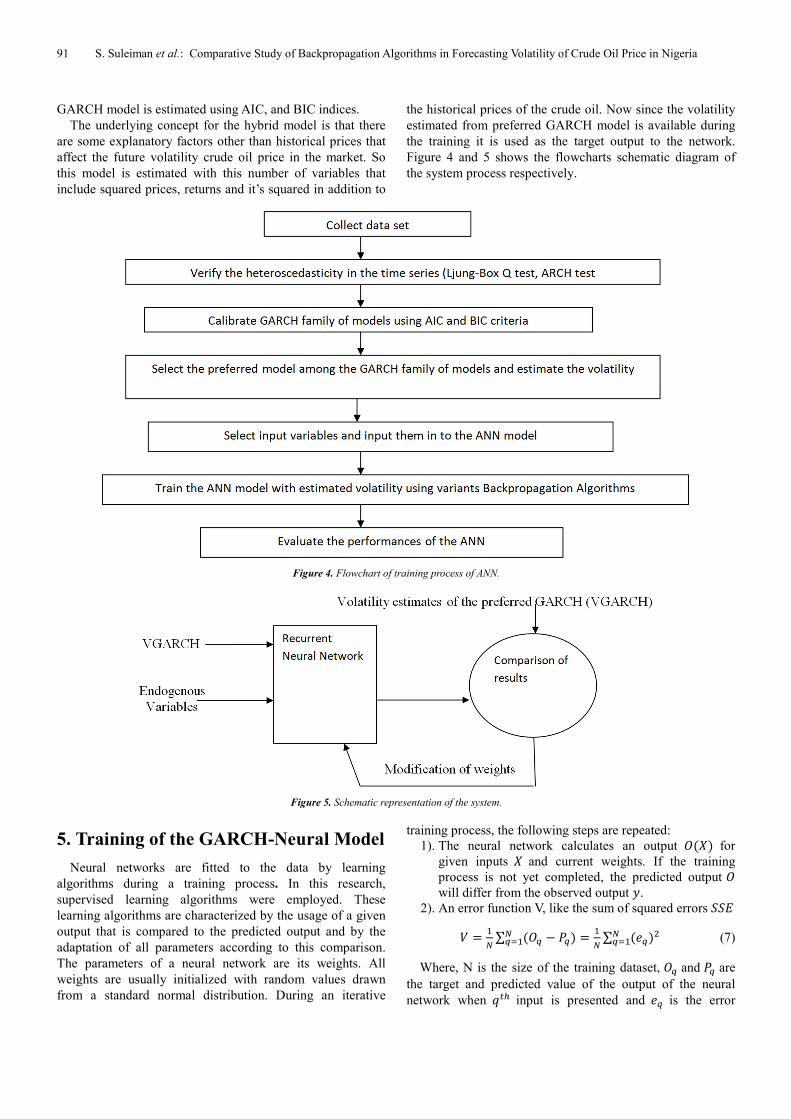
The underlying concept for the hybrid model is that there

are some explanatory factors other than historical prices that

affect the future volatility crude oil price in the market. So

this model is estimated with this number of variables that

include squared prices, returns and it’s squared in addition to

the historical prices of the crude oil. Now since the volatility

estimated from preferred GARCH model is available during

the training it is used as the target output to the network.

Figure 4 and 5 shows the flowcharts schematic diagram of

the system process respectively.

Figure 4. Flowchart of training process of ANN.

Figure 5. Schematic representation of the system.

5. Training of the GARCH-Neural Model

Neural networks are fitted to the data by learning

algorithms during a training process. In this research,

supervised learning algorithms were employed. These

learning algorithms are characterized by the usage of a given

output that is compared to the predicted output and by the

adaptation of all parameters according to this comparison.

The parameters of a neural network are its weights. All

weights are usually initialized with random values drawn

from a standard normal distribution. During an iterative

training process, the following steps are repeated:

1). The neural network calculates an output >�?� for

given inputs ? and current weights. If the training

process is not yet completed, the predicted output >

will differ from the observed output �.

2). An error function V, like the sum of squared errors @@2

A ��

B∑ �>� � C��

�

B∑ �D��B

��B�� (7)

Where, N is the size of the training dataset, >� and C� are

the target and predicted value of the output of the neural

network when E�F input is presented and D� is the error


(difference between the target and predicted value) for the

E�F input. The performance index V in (7) is a function of

weights and biases, G � [G� G� … GI] and can be given by

A(G) = �B ∑ D��(G)B�� (8)

The performance of the neural network can be improved

by modifying G till the desired level of the performance

index, A(G) is achieved. This is achieved by minimizing

A(G) with respect to G and the gradient required for this is given by

∇A(G) = LM(G)D(G) (9)

Where, L(G) is the Jacobian matrix given by

L(G) =NOOP ⋮

RST(U)RVT

… RST(U)RVW

⋱

RSY(U)RVT

… RSY(U)RVW

⋮Z[[\ (10)

and D(G) is the error for all the inputs. The gradient in (8) is determined using back propagation algorithms, which involves performing computations backward through the network. The process stops if a pre-specified criterion is fulfilled, i.e. if the values of the gradient are smaller than a given threshold.

This gradient is then used by different algorithms to update

the weights of the network. These algorithms differ in the

way they use the gradient to update the weights of the

network and are known as the variants of the back

propagation algorithms.

Gradient descent algorithm with other variants is discussed

below: Gradient Descent algorithms (GD): The network weights

and biases, G is modified in a direction that reduces the performance function in (8) most rapidly i.e. the negative of the gradient of the performance function [28]. The updated weights and biases in this algorithm are given by

G!]� = G! − �!∇A! (11)

Where, G! is the vector of the current weights and biases,

∇A! is the current gradient of the performance function and

�! is the learning rate.

Scaled Conjugate Gradient Descent algorithm (SCGD):

The gradient descent algorithm updates the weights and

biases along the steepest descent direction but is usually

associated with poor convergence rate as compared to the

Conjugate Gradient Descent algorithms, which generally

result in faster convergence [29], in the Conjugate Gradient

Descent algorithms, a search is made along the conjugate

gradient direction to determine the step size that minimizes

the performance function along that line. This time

consuming line search is required during all the iterations of

the weight update. However, the Scaled Conjugate Gradient

Descent algorithm does not require the computationally

expensive line search and at the same time has the advantage

of the Conjugate Gradient Descent algorithms [29]. The step

size in the conjugate direction in this case is determined

using the Levenberg-Marquardt approach. The algorithm

starts in the direction of the steepest descent given by the

negative of the gradient as

^_ = −∇A_ (12)

The updated and weights and biases are then given by

G!]� = G! + �!^! (13)

Where �! is the step size determined by the Levenberg-Marquardt algorithm [30]. The next search direction that is conjugate to the previous search directions is determined by combining the new steepest descent direction with the previous search direction and is given by

^! = −∇A! + �!^! � (14)

The value of �! is given in (Moller, 1993), by

�! = |∇`3aT|b ∇`3aT∇`3c3

(15)

Where �! is given by

�! = ^!d∇A! (16)

Levenberg-Marquardt algorithm (LM): Since the

performance index in (8) is sum of squares of non linear

function, the numerical optimization techniques for non

linear least squares can be used to minimize this cost

function. The Levenberg-Marquardt algorithm, which is an

approximation to the Newton’s method is said to be more

efficient in comparison to other methods for convergence of

the Backpropagation algorithm for training a moderate-sized

feedforward neural network [30]. As the cost function is a

sum of squares of non linear function, the Hessian matrix

required for updating the weights and biases need not be

calculated and can be approximated as

e = LM(G)L(G) (17)

The updated weights and biases are given by

G!]� = G! − [LM(G)L(G) + �#] �LM(G)D(G) (18)

Where � is a scalar and I is the identity matrix.

Automated Bayesian Regularization (BR): Regularization

as a mean of improving network generalization is used within

the Levenberg-Marquardt algorithm. Regularization involves

modification in the performance function. The performance

function for this is the sum of the squares of the errors and it

is modified to include a term that consists of the sum of

squares of the network weights and biases. The modified

performance function is given by

f"Sg = �@@2 + �@@h (19)

Where SSE and SSW are given by

@@2 = ∑ D��(G)B�� (20)

@@h = ∑ i��I

�� (21)


Where is the total number of weights and biases, i� in

the network. The performance index in (19) forces the

weights and biases to be small, which produces a smoother

network response and avoids over fitting. The values � and �

are determined using Bayesian regularization in an

automated manner [31] and [32].

6. Computational Results

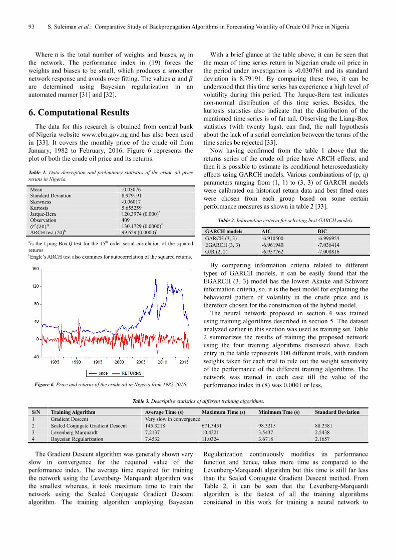
The data for this research is obtained from central bank

of Nigeria website www.cbn.gov.ng and has also been used

in [33]. It covers the monthly price of the crude oil from

January, 1982 to February, 2016. Figure 6 represents the

plot of both the crude oil price and its returns.

Table 1. Data description and preliminary statistics of the crude oil price

reruns in Nigeria.

Mean -0.03076 Standard Deviation 8.979191 Skewness -0.06017 Kurtosis 5.655259 Jarque-Bera 120.3974 (0.000)* Observation 409

j��20�k 130.1729 (0.0000)* ARCH test (20)b 99.629 (0.0000)*

ais the Ljung-Box j test for the 15th order serial correlation of the squared

returns bEngle’s ARCH test also examines for autocorrelation of the squared returns.

Figure 6. Price and returns of the crude oil in Nigeria from 1982-2016.

With a brief glance at the table above, it can be seen that

the mean of time series return in Nigerian crude oil price in

the period under investigation is -0.030761 and its standard

deviation is 8.79191. By comparing these two, it can be

understood that this time series has experience a high level of

volatility during this period. The Jarque-Bera test indicates

non-normal distribution of this time series. Besides, the

kurtosis statistics also indicate that the distribution of the

mentioned time series is of fat tail. Observing the Liang-Box

statistics (with twenty lags), can find, the null hypothesis

about the lack of a serial correlation between the terms of the

time series be rejected [33].

Now having confirmed from the table 1 above that the

returns series of the crude oil price have ARCH effects, and

then it is possible to estimate its conditional heteroscedasticity

effects using GARCH models. Various combinations of (p, q)

parameters ranging from (1, 1) to (3, 3) of GARCH models

were calibrated on historical return data and best fitted ones

were chosen from each group based on some certain

performance measures as shown in table 2 [33].

Table 2. Information criteria for selecting best GARCH models.

GARCH models AIC BIC

GARCH (3, 3) -6.910500 -6.996954

EGARCH (3, 3) -6.961940 -7.036414

GJR (2, 2) -6.957762 -7.008816

By comparing information criteria related to different

types of GARCH models, it can be easily found that the

EGARCH (3, 3) model has the lowest Akaike and Schwarz

information criteria, so, it is the best model for explaining the

behavioral pattern of volatility in the crude price and is

therefore chosen for the construction of the hybrid model.

The neural network proposed in section 4 was trained

using training algorithms described in section 5. The dataset

analyzed earlier in this section was used as training set. Table

2 summarizes the results of training the proposed network

using the four training algorithms discussed above. Each

entry in the table represents 100 different trials, with random

weights taken for each trial to rule out the weight sensitivity

of the performance of the different training algorithms. The

network was trained in each case till the value of the

performance index in (8) was 0.0001 or less.

Table 3. Descriptive statistics of different training algorithms.

S/N Training Algorithm Average Time (s) Maximum Time (s) Minimum Tme (s) Standard Deviation

1 Gradient Descent Very slow in convergence

2 Scaled Conjugate Gradient Descent 145.3218 671.3451 98.3215 88.2381

3 Levenberg Marquardt 7.2137 10.4321 3.5437 2.5438

4 Bayesian Regularization 7.4532 11.0324 3.6718 2.1657

The Gradient Descent algorithm was generally shown very

slow in convergence for the required value of the

performance index. The average time required for training

the network using the Levenberg- Marquardt algorithm was

the smallest whereas, it took maximum time to train the

network using the Scaled Conjugate Gradient Descent

algorithm. The training algorithm employing Bayesian

Regularization continuously modifies its performance

function and hence, takes more time as compared to the

Levenberg-Marquardt algorithm but this time is still far less

than the Scaled Conjugate Gradient Descent method. From

Table 2, it can be seen that the Levenberg-Marquardt

algorithm is the fastest of all the training algorithms

considered in this work for training a neural network to


forecast the volatility. Since the training time required for

different training algorithms have been compared, the

conclusion drawn from the results for the offline training

may also be extended to online training. Therefore, it can be

assumed that similar trend of training time required by the

different training algorithms will be exhibited during online

training of the proposed model for continuous updating of the

offline trained model.

Now the neural networks trained using the training

algorithms listed in table 2 were tested. The datasets used for

testing the networks were those points not included in the

training set. Twenty set of data was considered. As the

Gradient Descent algorithm was too low to converge for the

desired value of the performance index, the neural networks

that were trained using the rest of the three training algorithms

listed in table 2 were tested using the datasets. The results for

these are shown in the figures 7, 8 and 9 for Scale Conjugate

Gradient, Levenberg-Marquardt and Bayesian Regularization

respectively. The average absolute error is the least for the

neural network trained using the LM method.

Table 4. Performance of trained neural networks on the datasets.

S/No. Training Method Average Absolute Error for entire set Maximum Error Minimum Error

1 LM 0.001711 0.002901 0.000389

2 BR 0.04591 0.115341 0.0056

3 SCG 0.252393 0.506405 0.037923

Figure 7. Target and Predicted output of the GARCH-Neuron System using Scaled Conjugate Gradient.

Figure 8. Target and Predicted output of the GARCH-Neuron System using Levenberg-Marquardt.


Figure 9. Target and Predicted output of the GARCH-Neuron System using Bayesian Regularization.

7. Conclusion

A GARCH-Neural model has been proposed to forecast the

volatility of the crude oil price in Nigeria. In the first place, A

GARCH model was first identified upon which a hybrid model

is built. EGARCH (3, 3) was identified to be preferred model

for forecasting the volatility of crude oil price in Nigeria.

Variants of the Backpropagation were used to train the

proposed model. Investigations in to the training performance

of the different algorithms show that the Levenberg-Marquardt

(LM) algorithm is the fastest to converge. It was also

established that LM algorithm gives most accurate predictions

in comparisons to the target values of the volatility forecasted

earlier by the preferred GARCH models.

References

[1] Adamu A., (2015). The Impact of Global Fall in Oil Prices on the Nigerian Crude Oil Revenue and Its Prices, Proceedings of the Second Middle East Conference on Global Business, Economics, Finance and Banking Dubai-UAE, 22-24.

[2] Mgbame C. O., Donwa P. A., Onyeokweni O. V., (2015). Impact of oil price volatility on Economic growth: Conceptual perspective, International Journal of Multidisciplinary Research and Development 9, 80-85.

[3] Ogiri, I., H., Amadi, S., N., Uddin, M., M., & Dubon, P. (2013). Oil price and stock market performance in Nigeria: An empirical analysis. American Journal of Social and Management Sciences, 4 (1), 20–41.

[4] Oriakhi, D. E., & Osazee, I. D. (2013). Oil price volatility and its consequences on the growth of the Nigerian economy: An examination (1970-2010). Asian Economic and Financial Review, 3 (5), 683-702.

[5] Halpin, S. M. & Burch, R. F., (1997) “Applicability of neural networks to industrial and commercial power systems: a tutorial overview”, IEEE Trans. Industry Applications, Vol. 33, No. 5, pp 1355-1361.

[6] Hajizadeh E., Seifi A., Fazel Zarandi M. H., Turksen I. B., (2012). A hybrid modeling approach for forecasting the volatility of S&P 500 index return, Expert Systems with Applications, 39, 431-436.

[7] Roman, J., and A. Jameel, (1996) “Backpropagation and recurrent neural networks in financial analysis of multiple stock market returns,” Proceedings of the Twenty-Ninth Hawaii International Conference on System Sciences, Vol. 2, 1996, pp. 454–460.

[8] Monfared S. A., and Enke D., (2014) “Volatility Forecasting using a Hybrid GJR-GARCH Neural Network model”, Procedia Computer Science 36, 246-253.

[9] Donaldson R. G., and Kamstra M., (1997) “An artificial neural network-GARCH model for international stock return volatility”, Journal of Empirical Finance, vol. 4, no. 1, pp. 17-46.

[10] Mantri J. K., Gahan P., Nayak B. B., (2010) “Artificial Neural Networks - An Application to Stock Market Volatility”, International Journal of Engineering Science and Technology, vol. 2, no. 5, pp. 1451-1460.

[11] Jung-W. P., Venayagamoorthy, G. K., & Harley, R. G., (2005) “MLP/RBF neural networks based online global model identification of synchronous generator”, IEEE Trans. Industrial Electronics, Vol. 52, No. 6, pp1685- 1695.

[12] Venayagamoorthy, G. K., & Kalyani, R. P., (2005) “Two separate continually online-trained neurocontrollers for a unified power flow controller”, IEEE Trans. Industry Applications, Vol. 41, No. 4, pp 906-916.

[13] Mohamed, Y. A.-R., & El-Saadany, E. F., (2008) “Adaptive Discrete-Time Grid-Voltage Sensorless Interfacing Scheme for Grid-Connected DG-Inverters Based on Neural- Network Identification and Deadbeat Current Regulation”, IEEE Trans. Power Electronics, Vol. 23, No. 1, pp308-321.

[14] Tiwari, S., Naresh, R., & Jha, R., (2011) “Neural network predictive control of UPFC for improving transient stability performance of power system”, Appl Soft Comput, Vol. 11, No. 8, pp4581-4590.


[15] Engle, R. F., (1982). Autoregressive conditional heteroscedasticity with estimates of the variance of United Kingdom inflation, Econometrica, 50, 987-1007.

[16] Bollerslev, T. (1986). Generalized autoregressive conditional heteroscedasticity. Journal of Econometrics, 31, 307–327.

[17] Glosten, L. R. R. Jagannathan and D. Runkle. 1993. “On the Relation between the Expected Value and the Volatility of the Nominal Excess Return on Stocks.” Journal of Finance. 48, 1779-1801.

[18] Nelson, D. B. (1991). Conditional heteroskedasticity in asset returns: a new approach. Econo- metrica 59, 347-370.

[19] Longmore, R., and W. Robinson. 2004. “Modelling and Forecasting Exchange Rate Dynamics: An Application of Asymmetric Volatility Models”. Bank of Jamaica. Working Paper WP2004/03.

[20] Ding, Z. R. F. Engle and C. W. J. Granger. 1993. “Long Memory Properties of Stock Market Returns and a New Model”. Journal of Empirical Finance. 1. 83–106.

[21] Gupta M., Jin L., and Homma N., (2003) Static and Dynamic Neural Networks: From Fundamentals to Advanced Theory. New York: IEEE and Wiley.

[22] Werbos P. J., The Roots of Backpropagation. New York: Wiley, 1994.

[23] De Jesus, O. and M. T. Hagan, (2001a). Backpropagation through time for a general class of recurrent network. Proceedings of the international Joint Conference on Neural Networks, July 15-19, Washington, DC, USA., PP: 2638-2642.

[24] Roman, J., and A. Jameel, “Backpropagation and recurrent neural networks in financial analysis of multiple stock market returns,” Proceedings of the Twenty-Ninth Hawaii International Conference on System Sciences, Vol. 2, 1996, pp. 454–460.

[25] Kamwa, I., R. Grondin, V. K. Sood, C. Gagnon, Van Thich Nguyen, and J. Mereb, “Recurrent neural networks for phasor detection and adaptive identification in power system control and protection,” IEEE Transactions on Instrumentation and Measurement, Vol. 45, No. 2, 1996, pp. 657–664.

[26] Medsker, L. R., and L. C. Jain (2000), Recurrent neural networks: design and applications, Boca Raton, FL: CRC Press.

[27] Narendra, K. S., & Parthasarathy, K., (1990) “Identification and control of dynamical systems using neural networks”, IEEE Trans. Neural Networks, Vol. 1, No. 1, pp4-27.

[28] Hagan, M. T., Demuth, H. B., & Beale, M. H (1996) Neural Network Design, MA: PWS Publishing Boston.

[29] Moller, M. F., (1993) “A scaled conjugate gradient algorithm for fast supervised learning”, Neural Networks, Vol. 6, pp 525-533.

[30] Hagan, M. T., & Menhaj, M., (1994) “Training feed-forward networks with the Marquardt algorithm”, IEEE Trans. Neural Networks, Vol. 5, No. 6, pp989-993.

[31] Foresee, F. D. & Hagan, M. T., (1997) “Gauss-Newton approximation to Bayesian regularization”, International Joint Conference on Neural Networks.

[32] Mackay, D. J. C., (1992) “Bayesian interpolation”, Neural Computation, Vol. 4, No. 3, pp 415-447.

[33] S. U. Gulumbe, S. Suleiman, B. K. Asare and M. Abubakar. Forecasting Volatility of Nigerian Crude Price Using Non-linear Auto-Regressive with Exogenous (NARX) Inputs Model, imperial journal of interdisciplinary Research (IJIR), Vol. 2, Issue 5, pp 434-442.

comparative study of backpropagation algorithms in

Documents