algorithms and a software system for comparative …
TRANSCRIPT

Universitat Ulm
Abteilung Theoretische Informatik
Arbeitsgruppe Theoretische Bioinformatik
Leiter: Prof. Dr. Uwe Schoning
ALGORITHMS AND A SOFTWARE SYSTEM
FOR
COMPARATIVE GENOME ANALYSIS
DISSERTATION
zur Erlangung des Doktorgrades Dr. rer. nat.
der Fakultat fur Informatik der Universitat Ulm
vorgelegt von
MOHAMED MOSTAFA MOHAMED IBRAHIM ABOUELHODA
Ulm, 2005

Amtierender Dekan: Prof. Dr. H. Partsch
Gutachter: Prof. Dr. Enno Ohlebusch
Prof. Dr. Uwe Schoning
Prof. Dr. Robert Giegerich
Tag der Promotion: 13 Juli, 2005
University of Ulm
Theoretical Computer Science Department
Theoretical Bioinformatics Group
Chairman: Prof. Dr. Uwe Schoning
ALGORITHMS AND A SOFTWARE SYSTEM
FOR
COMPARATIVE GENOME ANALYSIS
A thesis submitted to the
Faculty of Computer Science of University of Ulm
in fulfillment of the requirements for
the degree of Doctor of Science Dr. rer. nat.
by
MOHAMED MOSTAFA MOHAMED IBRAHIM ABOUELHODA
Ulm, Germany
2005

Dean: Prof. Dr. H. Partsch
Reviewers: Prof. Dr. Enno Ohlebusch
Prof. Dr. Uwe Schoning
Prof. Dr. Robert Giegerich
Day of Conferral of Doctorate: 13 July 2005
Acknowledgments
Foremost, I am grateful to my supervisor, Enno Ohlebusch. His con-tinuous support and guidance have greatly influenced my doctoral studies,research, and this work. I am sure that his teachings will always accompanyme in the trip of scientific research. I am grateful to Robert Giegerich forintroducing the problem to me, and for refereeing the thesis. His invalu-able discussions and suggestions have been reflected in many places in thisresearch. Thanks to Uwe Schoning for reading the whole thesis and referee-ing it. My gratitude to Stefan Kurtz for the fruitful discussions that alwaysattracted my attention to many practical aspects of sequence analysis.
I am thankful to Dirk Strothmann for his fruitful observations that haveimproved parts of this research, and to Janina Reeder for providing me withpieces of codes. I also thank Michael Beckstette and Alexander Sczyrba fordiscussions about the suffix array and cDNA/EST mapping. My thanks goalso to Kathrin Hockel, Jan Stallkamp, Randall Pruim, and Jakir H. Ullahfor their careful readings and the helpful comments to improve this script.
I am always indebted to my teachers, from school to university, but un-fortunately the few pages I am restricted to are not enough to mention themall. Although they were not directly involved in this work, their teachingshave influenced and will influence my research and life.
Finally, I am indebted to my parents, my wife, and my family for theirlove, encouragement, and support.
This work was supported by Graduiertenkolleg Bioinformatik, Bielefeld,and by DFG-grant Oh 53/4-1.


Contents
1 Introduction 11.1 Comparative genomics . . . . . . . . . . . . . . . . . . . . . . 11.2 This Thesis . . . . . . . . . . . . . . . . . . . . . . . . . . . . 3
1.2.1 The enhanced suffix arrays . . . . . . . . . . . . . . . . 31.2.2 The chaining algorithms . . . . . . . . . . . . . . . . . 41.2.3 Publications . . . . . . . . . . . . . . . . . . . . . . . . 61.2.4 Implementations . . . . . . . . . . . . . . . . . . . . . 61.2.5 Thesis Organization . . . . . . . . . . . . . . . . . . . 6
2 The Genome 92.1 DNA: The molecule of life . . . . . . . . . . . . . . . . . . . . 92.2 Structure of eukaryotic genomes . . . . . . . . . . . . . . . . . 11
2.2.1 Overview . . . . . . . . . . . . . . . . . . . . . . . . . 112.2.2 Chromosomes . . . . . . . . . . . . . . . . . . . . . . . 122.2.3 Genes . . . . . . . . . . . . . . . . . . . . . . . . . . . 142.2.4 Intergenic regions . . . . . . . . . . . . . . . . . . . . . 18
2.3 Structure of prokaryotic genomes . . . . . . . . . . . . . . . . 202.3.1 Overview . . . . . . . . . . . . . . . . . . . . . . . . . 202.3.2 The main genome . . . . . . . . . . . . . . . . . . . . . 202.3.3 Genes . . . . . . . . . . . . . . . . . . . . . . . . . . . 202.3.4 Intergenic regions . . . . . . . . . . . . . . . . . . . . . 21
2.4 Genome dynamics and evolution . . . . . . . . . . . . . . . . . 212.5 Comparative genomics and perspectives . . . . . . . . . . . . . 23
3 Comparative Genomics Tools: A Survey 273.1 Sequence alignment algorithms . . . . . . . . . . . . . . . . . 283.2 Classification scheme of the methods . . . . . . . . . . . . . . 31
3.2.1 The semi-manual strategy . . . . . . . . . . . . . . . . 313.2.2 The window-based strategy . . . . . . . . . . . . . . . 323.2.3 The anchor-based strategy . . . . . . . . . . . . . . . . 33
3.3 Techniques in the anchor-based strategy . . . . . . . . . . . . 33
i

CONTENTS
3.3.1 Fragment generation techniques . . . . . . . . . . . . . 333.3.2 Anchors finding techniques . . . . . . . . . . . . . . . . 38
3.4 The tools . . . . . . . . . . . . . . . . . . . . . . . . . . . . . 423.4.1 WABA . . . . . . . . . . . . . . . . . . . . . . . . . . . 423.4.2 PipMaker and BLASTZ . . . . . . . . . . . . . . . . . 433.4.3 LSH-ALL-PAIRS . . . . . . . . . . . . . . . . . . . . . 453.4.4 ASSIRC . . . . . . . . . . . . . . . . . . . . . . . . . . 463.4.5 DIALIGN . . . . . . . . . . . . . . . . . . . . . . . . . 463.4.6 GLASS . . . . . . . . . . . . . . . . . . . . . . . . . . 483.4.7 AVID . . . . . . . . . . . . . . . . . . . . . . . . . . . 483.4.8 CHAOS and LAGAN . . . . . . . . . . . . . . . . . . . 493.4.9 MUMmer . . . . . . . . . . . . . . . . . . . . . . . . . 513.4.10 MGA . . . . . . . . . . . . . . . . . . . . . . . . . . . . 523.4.11 Very recent tools: EMAGEN and Mauve . . . . . . . . 53
3.5 Remarks on the surveyed techniques . . . . . . . . . . . . . . 543.5.1 Choice of fragments . . . . . . . . . . . . . . . . . . . . 543.5.2 Setting of parameters . . . . . . . . . . . . . . . . . . . 553.5.3 The multiple alignment methods . . . . . . . . . . . . 55
3.6 Conclusions . . . . . . . . . . . . . . . . . . . . . . . . . . . . 56
4 The Enhanced Suffix Array 614.1 Basic notions . . . . . . . . . . . . . . . . . . . . . . . . . . . 614.2 The suffix tree and the suffix array . . . . . . . . . . . . . . . 614.3 The enhanced suffix array . . . . . . . . . . . . . . . . . . . . 64
4.3.1 Basic concepts and definitions . . . . . . . . . . . . . . 644.3.2 Applications . . . . . . . . . . . . . . . . . . . . . . . . 65
4.4 Algorithms based on properties of the enhanced suffix arrays . 664.4.1 Repeat analysis and genome comparison . . . . . . . . 664.4.2 The lcp-intervals . . . . . . . . . . . . . . . . . . . . . 674.4.3 Computation of supermaximal repeats . . . . . . . . . 684.4.4 Computation of maximal unique matches . . . . . . . . 69
4.5 Bottom-up traversals . . . . . . . . . . . . . . . . . . . . . . . 704.5.1 The lcp-interval tree of a suffix array . . . . . . . . . . 714.5.2 Computation of maximal repeated pairs . . . . . . . . 734.5.3 Computation of maximal exact matches . . . . . . . . 754.5.4 Computation of maximal multiple exact matches . . . 784.5.5 Other applications of the bottom-up traversal . . . . . 78
4.6 Top-down traversals . . . . . . . . . . . . . . . . . . . . . . . 834.6.1 Exact pattern matching . . . . . . . . . . . . . . . . . 844.6.2 Other applications of the top-down traversal . . . . . . 90
4.7 Incorporating suffix links . . . . . . . . . . . . . . . . . . . . . 92
ii

CONTENTS
4.7.1 Suffix links . . . . . . . . . . . . . . . . . . . . . . . . 924.7.2 Space efficient computation of MEMs . . . . . . . . . . 97
4.8 Implementation details . . . . . . . . . . . . . . . . . . . . . . 1024.8.1 The lcp-table . . . . . . . . . . . . . . . . . . . . . . . 1024.8.2 The child-table . . . . . . . . . . . . . . . . . . . . . . 1034.8.3 The suffix link table . . . . . . . . . . . . . . . . . . . 103
4.9 Experimental results . . . . . . . . . . . . . . . . . . . . . . . 1044.9.1 Algorithms based on properties of enhanced suffix arrays1054.9.2 Algorithms based on bottom-up traversal . . . . . . . . 1064.9.3 Algorithms based on top-down traversal . . . . . . . . 1084.9.4 Algorithms for traversals using suffix links . . . . . . . 110
4.10 Conclusions and future perspectives . . . . . . . . . . . . . . . 111
5 Chaining Algorithms 1155.1 Introduction . . . . . . . . . . . . . . . . . . . . . . . . . . . . 1155.2 Basic concepts and definitions . . . . . . . . . . . . . . . . . . 1165.3 The global chaining problem . . . . . . . . . . . . . . . . . . . 118
5.3.1 Graph based formulation . . . . . . . . . . . . . . . . . 1185.3.2 Geometric based formulation . . . . . . . . . . . . . . . 119
5.4 Two dimensional global chaining without gap costs . . . . . . 1215.4.1 The Basic chaining algorithm . . . . . . . . . . . . . . 1215.4.2 Answering RMQ with activation . . . . . . . . . . . . . . 122
5.5 Higher dimensional chaining without gap costs . . . . . . . . . 1265.5.1 Chaining with range trees . . . . . . . . . . . . . . . . 1275.5.2 Chaining with kd -trees . . . . . . . . . . . . . . . . . . 132
5.6 Incorporating gap costs into the algorithm . . . . . . . . . . . 1355.6.1 Costs in the L1 metric . . . . . . . . . . . . . . . . . . 1365.6.2 The sum-of-pairs gap cost . . . . . . . . . . . . . . . . 138
5.7 Local chaining: a basic variation . . . . . . . . . . . . . . . . . 1435.8 Variations . . . . . . . . . . . . . . . . . . . . . . . . . . . . . 145
5.8.1 Including gap constrains . . . . . . . . . . . . . . . . . 1465.8.2 cDNA/EST mapping . . . . . . . . . . . . . . . . . . . 148
5.9 Related problems . . . . . . . . . . . . . . . . . . . . . . . . . 1495.9.1 1-dimensional chaining . . . . . . . . . . . . . . . . . . 1495.9.2 A more general problem . . . . . . . . . . . . . . . . . 151
5.10 Conclusions . . . . . . . . . . . . . . . . . . . . . . . . . . . . 152
6 CHAINER: the software system 1556.1 Introduction . . . . . . . . . . . . . . . . . . . . . . . . . . . . 1556.2 Finding regions of high similarity . . . . . . . . . . . . . . . . 157
6.2.1 Detecting transposition events . . . . . . . . . . . . . . 157
iii
CONTENTS
6.2.2 Detecting inversions . . . . . . . . . . . . . . . . . . . 1586.2.3 A large scale comparison between the human and mouse
genomes . . . . . . . . . . . . . . . . . . . . . . . . . . 1606.3 Multiple global alignment . . . . . . . . . . . . . . . . . . . . 1626.4 Comparing draft genomes . . . . . . . . . . . . . . . . . . . . 1626.5 cDNA mapping . . . . . . . . . . . . . . . . . . . . . . . . . . 1656.6 Parameter Estimation . . . . . . . . . . . . . . . . . . . . . . 166
6.6.1 Parameters for comparing genomes . . . . . . . . . . . 1676.6.2 Parameters for cDNA/EST mapping . . . . . . . . . . 169
6.7 Conclusions . . . . . . . . . . . . . . . . . . . . . . . . . . . . 169
7 Conclusions 171
Bibliography 176
iv
Chapter 1
Introduction
1.1 Comparative genomics
It was not until the middle of the last century that DNA was conclusivelyrecognized as the genetic material of living organisms. In 1953, Watson andCrick unraveled the physical structure of the DNA molecule and explainedits underlying biological implications. Undoubtedly, this contribution was amajor breakthrough in biology during the 20th century. Another remarkablemilestone in the rise of modern biology is the advent of sequencing technolo-gies for determining the sequence of nucleotides composing a stretch of DNA(a nucleotide in DNA, as will be shown in the next chapter, is a chemical unitof the type A, C, G, or T). By means of this technology, biologists becameable to sequence longer and longer stretches of DNA so that in 1984 the se-quencing of the human genome became conceivable [30] (the genome is theentire DNA content of an organism). In 1995, these sequencing endeavorsculminated in sequencing the complete bacterial genome of H. influenza [53].This precursor success brought forth an extensive series of similar initiatives,most notably the sequencing of the first eukaryotic genome of S. cerevisiaein 1996 [58], and lent more support towards the completion of the humangenome project. The human genome project was an unprecedented world-wide collaboration that started in 1990 and its primary success, sequencing83-84% of the human genome, was announced in 2001 [72, 135] as the firstbreakthrough of the 21st century.
Presently, one speaks about the post-genomic era referring to the avail-ability of complete genomic sequences. To date (March 2005), the pub-lic databases contain complete genomes of more than 260 organisms (186genomes in April 2004) and about 1000 viruses [27]. In addition, more than1000 sequencing projects are on-going. In fact, the notion of post-genomic
1
CHAPTER 1. INTRODUCTION
era goes beyond the availability of newly sequenced genomes. It extends tocover those concepts and approaches that gradually change as more genomesbecome available. In the pre-genomic era the studies were solely handlingone or few genes of a certain organism. In the post-genomic era, scientistscan perform high throughput experiments over entire gene sets of completegenomes. It is this global view that actually characterizes the post-genomicera. It has enabled scientists to tackle puzzling questions and, at the sametime, enabled them to emphasize or even reconsider claims that were takenfor granted in the pre-genomic era. Scrutinizing the recent literature, onecan find many examples demonstrating this revolution.
At the outset of sequencing the human genome, scientists indicated theneed to sequence genomes of other organisms, especially those that can beexperimentally manipulated in lab [115]. These organisms, known as modelorganisms, included bacteria (most notably E. coli), the yeast S. cerevisiae,the fruit fly D. melanogaster, the roundworm C. elegans, and the laboratorymouse M. musculus. The objectives were several: (1) to represent throughthese model organisms a wide range of life forms, (2) to elucidate the func-tion of human DNA segments, such as genes, by performing experiments inthese organisms using the segments themselves (by inserting them into themodel genome) or their counterparts already existing in the model genome,and (3) to put forward an explanation for unexpected genomic puzzles, suchas gene structure and genome organization, that have taken scientists by sur-prise. Before finishing the human genome project, many of these genomesbecame available. Accordingly, comparative sequence analysis of the humangenome with those of these model organisms has been applied as an im-mensely valuable tool to identify regions of similarity and difference amonggenomes. These comparisons have already provided critical clues about thestructure and function of many genomic segments, which, in many respects,have helped approach the objectives. However, these model organisms, es-pecially because they include few advanced ones, have not been able to pro-vide enough information to satisfactorily achieve the objectives. Thus, moregenomes are being sequenced.
With the ever-increasing number of genomes becoming available, com-parative genomics has been heralded as the next logical step towards under-standing how genomes organize, function, replicate, and evolve. In additionto these basic research topics, comparative genomics has already started toplay an essential role in the fields of biotechnology and pharmaceutical in-dustries. The range of its application includes, among others, improving theproductivity of certain organisms, the design of diagnostic probes specific to acertain kind of microbes, and the identification of potential targets (proteinsor DNA) onto which drugs can act.
2
CHAPTER 1. INTRODUCTION
In the pre-genomic era, computer scientists and engineers were involved inmanipulating biological data and performing limited scale analysis includingsome genome segments or isolated genes. In the post-genomic era, computerscientists are demanded, more than before, by the biological scientific com-munity to develop software tools that are able to cope with the shear volumeof the available data, particularly for the purpose of analyzing and comparingcompletely sequenced genomes. This has given rise to computational com-parative genomics as a growing field of bioinformatics. Giving it a definition,computational comparative genomics is the field concerned with analyzinggenomic sequences by comparing them to one another. This field involves theapplication of high-throughput computational techniques, the application ofdata mining and statistical hypothesis testing, the development of novel al-gorithms for new problems, and the re-design of traditional algorithms thatare not efficient enough for handling large scale analysis in the post-genomicera.
1.2 This Thesis
The thesis at hand presents algorithms for large scale analysis and comparisonof genomic sequences. The algorithms presented here can be broadly dividedinto two categories. The first includes algorithms that analyze large genomicsequences based on indexing data structures. The second includes algorithmsfor comparing two or more genomes.
1.2.1 The enhanced suffix arrays
For analyzing large genomic sequences, we introduce the enhanced suffix ar-rays, an indexing data structure on which the algorithms of the first cat-egory are based. The suffix array of a sequence S of n characters (eachcharacter represents a nucleotide) is a table storing the starting positions ofthe lexicographically-ordered suffixes of S. The suffix array was introducedabout 10 years ago [59, 100] as a more space-efficient data structure for an-swering “on-line queries” than the suffix tree. The suffix tree is a traditionalindexing data structure that is used for a myriad of sequence analysis ap-plications [62, 101, 137]. Although the suffix tree plays a prominent role inalgorithmics, it is not as wide spread in actual implementations of softwaretools as one should expect. This is because of its large space consumption; ittakes, in the worst case, 20n bytes (20 bytes per one character of the inputsequence). The suffix array, on the other hand, requires only 4n bytes. How-ever, since the time of its introduction, the suffix array had been thought of
3
CHAPTER 1. INTRODUCTION
as a less efficient data structure than the suffix tree. The reasons for this weremanifold: (1) For a string S of length n, the then presented suffix array con-struction algorithm had the time complexity of O(n logn), while the suffixtree can be constructed in linear time. (2) The only known algorithm on thesuffix array was for answering on-line queries of the type “Is P a substringof S?”. This algorithm had time complexity of O(m + log n), while thatalgorithm based on suffix trees has time complexity of O(m), where m is thelength of P . Worse, it was not clear whether the other problems that hadalready been solved using the suffix tree could also be solved using the suffixarray; and if so, how the efficiency of the suffix array based algorithms wouldcompare to that of their suffix tree counterparts. Although the suffix arrayconstruction algorithms were further improved so that they became moreefficient than those that construct suffix trees, there was a lingering doubtabout the eligibility of the suffix array, as a data structure, for performingsequence analysis tasks. Our enhanced suffix arrays have laid this doubt torest.
The enhanced suffix array of a sequence S is basically the suffix array ofS but enhanced with additional information (tables). With the help of thesetables, we show that every algorithm on the suffix tree can be systematicallyreplaced with an equivalent one on the enhanced suffix array without loss ofefficiency. That is, our algorithms have the same time complexity as thosealgorithms developed for the suffix tree. To take one example, the aforemen-tioned query of the type “Is P a substring of S?” can now be answered inO(m) time using the enhanced suffix array. Furthermore, we present a setof algorithms that exploit solely the properties of the enhanced suffix arrays.Depending on the application at hand, the enhanced suffix array requires,in practice, 5n to 7n bytes. Despite this space reduction, experimental re-sults show that our enhanced suffix array based algorithms are not only morespace-efficient, but also many times faster than the corresponding ones basedon the suffix tree.
1.2.2 The chaining algorithms
The second category of the algorithms presented in this thesis involves thosethat solve different comparative genomic tasks. These tasks include findinghomologous (similar) regions between two or multiple genomes, alignmentof two or more whole genomes, comparison of draft genomes, and mappingcDNA sequences to genomic sequences.
The problem of comparing complete genomes was addressed after thefirst bacterial genomes had become available. Before then, the comparisontasks had involved only sets of genes or parts of genomes. For this limited
4
CHAPTER 1. INTRODUCTION
scale analysis, computer scientists had presented dynamic programming algo-rithms, including many variations, to compare genomic sequences. However,these traditional dynamic programming algorithms, which run in time pro-portional to the product of the lengths of the sequences, could not keep pacewith the longer genomic sequences becoming available. To overcome thisdrawback that faced the newly sequenced genomes, several software toolswere (quickly) developed; some of these tools were semi-manual and the oth-ers used either naive and/or ad-hoc approaches. These tools were neithertime-efficient nor considered robust enough to produce reliable comparisonsin general. Gradually, several improved strategies were proposed. The mostprominent one was the anchor based strategy, which was originally introducedto speed up searching genomic databases [12, 116].
The anchor based strategy is composed of three phases:
1. Generating a set of fragments (regions of similarity) among the givengenomes.
2. Finding certain sets of non-overlapping fragments, which are calledanchors.
3. Applying standard dynamic programming technique or the same pro-cedure recursively on the regions between the anchors.
We improve and extend the anchor based strategy in several directions:First, for phase one, we show how to efficiently compute different kinds offragments using the enhanced suffix arrays. Second, for phase two, we in-troduce our chaining algorithms to determine the anchors. Our chainingalgorithms are versatile and can be readily used for the comparison of morethan two genomic sequences. For example, for producing global alignmentsof two or multiple genomes, we compute an optimal global chain of colin-ear non-overlapping fragments, while for finding homologous local regions,we compute significant local chains of colinear non-overlapping fragments.Third, we introduce additional variations of the chaining algorithms. Thesevariations extend the anchor based strategy to perform more comparative ge-nomics tasks, such as mapping a cDNA/EST database to genomic sequencesand comparing draft genomes.
Despite having these variations, all our chaining algorithms are optimizedusing techniques from the field of computational geometry so that they runin subquadratic time and space (in terms of the number of fragments). Ex-perimental results show that our chaining algorithms can handle millions offragments from two or more genomes in few minutes.
5

CHAPTER 1. INTRODUCTION
Overall, our algorithms based on the enhanced suffix array and our chain-ing algorithms compose an efficient tool that can compare two or multiplegenomes in few minutes; a task that took days using previous tools.
1.2.3 Publications
Parts of our contributions regarding the enhanced suffix array have beenpublished in [1, 2, 8]. Parts of our contribution regarding the chaining algo-rithms have been published in [3, 4, 6]. The implementation of our algorithmsand the system that integrates them have been published in [5]. Moreover,two book chapters will appear in the Handbook of Computational MolecularBiology [7, 113].
It is worth mentioning that our published data structures and algorithmshave recently been used in various software tools, such as e2g [88], PROBE-mer [49], EMAGEN [46], and PoSSuM [20].
1.2.4 Implementations
The enhanced suffix array and the fragment generation algorithms are im-plemented within the module Multimat of the Vmatch package [90] and thechaining algorithms are implemented in the software system CHAINER [5].The system also integrates the fragment generation algorithms and the chain-ing algorithms to solve versatile comparative genomics tasks. The softwaresystem CHAINER will be described in detail within this thesis. Our algo-rithms are available for free for educational and academic purposes.
1.2.5 Thesis Organization
In the following chapter, we will introduce the basic notions and concepts ofgenomics–the field of biological science dealing with complete genomes. Wewill recall the structure and organization of a genome. We will also give anaccount of the basic differences between eukaryotic and prokaryotic genomes.Furthermore, the basic concepts of genome dynamics and evolution will beaddressed. Finally, we will enumerate some of the potentials and perspectivesof comparative genomics.
In Chapter 3, we will present a survey of the software tools used in com-paring complete genomes. In this survey, we review the computational as-pects used in these tools, and use them as a basis for classifying the tools.Moreover, we will mention the advantages and disadvantages of each com-putational technique, and the scope of application where such a tool can bebest employed. A basic conclusion of this survey is that the anchor-based
6

CHAPTER 1. INTRODUCTION
strategy became the state of the art technique of computational comparativegenomics, and our algorithms, presented in the remaining chapters of thisthesis, significantly contribute to improving the efficiency of this strategyand widening its scope of applications.
In Chapter 4, we will present our enhanced suffix arrays. In this chapter,we will first recall the basic notions and definitions of the related suffix treeand the original suffix array (without enhancement). Then we will introducethe enhanced suffix array. We will explore its properties, and show how someproblems can be solved by solely exploiting these properties. Moreover, wewill show how any problem solved using the suffix tree can also be solvedusing the corresponding enhanced suffix array in the same time and spacecomplexity. Finally, we will prove by experiments that the enhanced suffixarray is not only of theoretical interest but also efficient in practice, and evensuperior to the suffix tree for handling large genomic data.
Chapter 5 presents our chaining algorithms. The chaining algorithms con-tribute to the second phase of the anchor-based strategy. In this chapter, wewill show how our chaining algorithms can be used in solving the global align-ment problem, and the local alignment problem for large genomes. Moreover,we will present a number of variations that can be used to solve other prob-lems, such as comparing draft genomes and mapping cDNA/EST (a kind ofgenomic sequences presented in this chapter) to a genomic sequence.
Finally, Chapter 6 presents our software system CHAINER. In this chap-ter, we show how the algorithms of Chapters 4 and 5 can be integrated ina single software system. We will demonstrate how this system is used tocompare two or multiple genomes, to detect genome rearrangements such asinversions, transpositions, and translocations. We will present the modes ofcomparing draft genomes and mapping a cDNA/EST database to a genomicsequence. Finally, we will address the problem of estimating the systemparameters.
The concluding section of each of these chapters summarizes the resultsobtained in the chapter, the related open problems, and the future work.
7

Chapter 2
The Genome
In this chapter, we give a brief overview of the basic biological conceptsand definitions required for explaining our algorithms. For a more detaileddescription of the biological processes involved, we refer the interested readerto [11, 30, 72, 73, 98, 135].
2.1 DNA: The molecule of life
Biologists divide the forms of life into two categories: cellular and non-cellular. Cellular life form includes all living organisms composed of cells.Non-cellular life forms, namely viruses, are merely genetic information sur-rounded by a protein coat. Viruses, by most definitions, are not alive becausethey neither self-reproduce nor metabolize. Cellular organisms are classifiedaccording to the cell type into eukaryotes and prokaryotes. A eukaryotic cell isdistinguished from a prokaryotic one by the existence of membrane-boundedcompartments (organelles) such as nucleus, mitochondrion, and chloroplast.A prokaryotic cell is simply molecules surrounded by a cell wall, and lacksthese extensive internal membrane-bounded compartments. While eukary-otes are classified into four basic kingdoms: animals, plants, protozoa, andfungi, prokaryotes are classified into only two kingdoms: bacteria and archae.
Every organism possesses a genome that encodes the biological informa-tion needed for its existence and reproduction. The genomes of all organismsthat belong to the cellular life form, including the human genome, are madeup of DNA (Deoxyribonucleic Acid). Genomes of many viruses, however,are made up of RNA (Ribonucleic Acid). A DNA molecule consists of twostrands that wrap around each other to resemble a twisted ladder, a struc-ture that is called the double helix, see Figure 2.1. Each strand is a polymericmolecule made up of a linearly arranged chain of monomeric subunits called
9

CHAPTER 2. THE GENOME
Figure 2.1: The structure of DNA. Each nucleotide is composed of a sugar
(S), a phosphate group (P), and a nitrogenous base of the type A, C, G, or
T. (Figure is redrawn from the National Health Museum Graphics Gallery,
http://www.accessexcellence.org/AB/GG.)
nucleotides. Each nucleotide is composed of deoxyribose sugar, a phosphategroup, and a nitrogenous base. A nucleotide is specified by the nitrogenousbase it contains. DNA contains four types of nitrogenous bases: adenine (A),thymine (T), cytosine (C), and guanine (G). The particular linear order inwhich the nucleotides are arranged is called the DNA sequence; this sequencespecifies the exact genetic instructions required to produce a particular or-ganism and maintain its own unique traits. The two strands of the DNA arecomplementary to each other. From one end to the other, every C in onestrand meets G in the second, and every A meets T, and vice versa. Thetwo DNA strands are held together by bonds joining every base to its com-plementary one on the opposite strand, this bonding forms base pairs (bp).As shown in Figure 2.1, the two ends of a strand are chemically distinct:one end has a phosphate group and the other has a sugar. The informationencoded on one strand is chemically uni-direction: it streams (processed bythe enzymes that function on the DNA) in the phosphate-to-sugar direction.This implies that the information flows on the other strand in the reversedirection. Therefore, one of the strands is called forward or positive and theother is called opposite, reverse complement, or minus strand.
10
CHAPTER 2. THE GENOME
Genome size is usually stated as the total number of base pairs (bp); thehuman genome, for instance, contains roughly 3 billion bp. This base pairinghas two implications: First, it stabilizes the physical structure of the doublehelix. Second, it makes it possible to produce exact copies of a master DNAsequence. The initial step in this copying process is that the two strandsunwind and separate. Then each strand works as a template that directs thesynthesis of a new complementary strand; where the free nucleotides in themedium are chained one after another in the new strand according to thecomplementary bases in the parent strand. Note that the replicating strandselongate in opposite directions to each other (the replicating enzymes workonly in the phosphate-to-sugar direction). By means of this mechanism,the whole genome of a parent cell replicates to two genomes (exact copies)whenever the cell undergoes meiotic division. Each child cell receives one ofthese genomes.
RNA is also a polymeric molecule but it is single-stranded. RNA nu-cleotides are made up of ribose sugar, and have the same nitrogenous basesas DNA except that the thymine (T) is replaced with uracil (U). RNA canalso form base pairs: the base A pairs with U and G pairs with C. But thispairing is intramolecular resulting in folded structures. This structure di-rectly influences the activity of the RNA molecule. RNA molecules existalso in genomes of prokaryotes and eukaryotes, but they are not part of thegenome. We will see soon that they are themselves encoded on the DNAgenome and expressed as genes that play various roles in the cell.
2.2 Structure of eukaryotic genomes
2.2.1 Overview
A eukaryotic genome is distributed over three organelles: nucleus, mitochon-drion, and chloroplast. The part of the genome that settles in the nucleusis called nuclear genome and the other parts outside the nucleus are calledorganelle (mitochondria/chloroplasts) genomes. The chloroplast genome ex-ists only in plants and photosynthetic organisms. The nuclear genome isthe basic genome, while the organelle genomes are much smaller and encodevery few genes. The human mitochondrial genome, for example, has 16568bp, which is a very small number compared to the 3 billion bp of the nucleargenome. Because of the similarity of organelle genomes to bacterial genomes,it is widely believed that both mitochondria and chloroplasts have evolvedfrom bacteria (rickettsia in case of mitochondria and cyanobacteria in caseof chloroplasts) living within their eukaryotic host cells at the very earliest
11
CHAPTER 2. THE GENOME
stages of evolution. This is postulated by what is known as the endosymbionttheory. The following discussion handles basically the nuclear genome.
The genome size varies significantly in different eukaryotes. The smalleststudied eukaryotic genome is less than 10 million bp and the largest studiedone is over 100 billion bp. Generally, the genome size increases with thecomplexity of the organism. The simplest eukaryotes, such as the fungi inthe protozoa kingdom, have the smallest genomes, while the higher ones,such as vertebrates and plants, have the largest ones. Nevertheless, somesurprising cases have been discovered. For example, the human genome (3billion bp) contains at least 250 times more DNA than the yeast genome(12 million bases), but it is much smaller than that of the Amoeba dubia(200 billion bp), which is also a protozoan unicellular creature as simple asyeast. In the pre-genomic era, this was looked on as a bit of puzzle. Bysequencing projects, it turned out that these large genomes contain a largeamount of repetitions; which suggests that repeats have undergone a massiveproliferation in the genomes of certain species (repeats will be addressed laterin this chapter).
2.2.2 Chromosomes
The nuclear genome is split into many units called chromosomes; all eu-karyotes that have been studied so far have at least two chromosomes. Thehuman nuclear genome of somatic cells, for example, contains 46 chromo-somes: 2 sex chromosomes (X and Y), and 22 pairs of homologous (similar)autosome chromosomes (one copy of the pair is maternal and the other ispaternal); i.e., there are 24 distinct chromosomes. Human chromosomes arenot of equal sizes: the smallest one is chromosome 21 (45 million bp), andthe largest one is chromosome 1 (279 million bp). The number of chromo-somes differs significantly in different organisms, and it appears to be neitherrelated to the organism complexity nor to the genome size. For example, theyeast has 16 chromosomes while the fruit fly has only 4, and some salaman-ders have genomes 30 times bigger than that of humans but with half thenumber of chromosomes.
Chromosomes are much shorter than the DNA they contain: the DNAmolecule of an average human chromosome is about 5 cm long. Therefore,the DNA must be packaged into a tiny space. This is achieved by a packagingsystem, where the DNA molecule is wound around DNA-binding proteins,called histones. After many levels of packaging, the DNA-molecule is even-tually fit into its cytologically visible unit: the chromosome; see Figure 2.2.It is now known that the nature of this packaging has a direct influence onthe processes involved in the genome activity. This piece of knowledge is
12
CHAPTER 2. THE GENOME
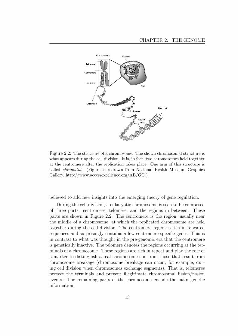
Figure 2.2: The structure of a chromosome. The shown chromosomal structure iswhat appears during the cell division. It is, in fact, two chromosomes held togetherat the centromere after the replication takes place. One arm of this structure iscalled chromatid. (Figure is redrawn from National Health Museum GraphicsGallery, http://www.accessexcellence.org/AB/GG.)
believed to add new insights into the emerging theory of gene regulation.
During the cell division, a eukaryotic chromosome is seen to be composedof three parts: centromere, telomere, and the regions in between. Theseparts are shown in Figure 2.2. The centromere is the region, usually nearthe middle of a chromosome, at which the replicated chromosome are heldtogether during the cell division. The centromere region is rich in repeatedsequences and surprisingly contains a few centromere-specific genes. This isin contrast to what was thought in the pre-genomic era that the centromereis genetically inactive. The telomere denotes the regions occurring at the ter-minals of a chromosome. These regions are rich in repeat and play the role ofa marker to distinguish a real chromosome end from those that result fromchromosome breakage (chromosome breakage can occur, for example, dur-ing cell division when chromosomes exchange segments). That is, telomeresprotect the terminals and prevent illegitimate chromosomal fusion/fissionevents. The remaining parts of the chromosome encode the main geneticinformation.
13

CHAPTER 2. THE GENOME
2.2.3 Genes
Gene structure
Each chromosome hosts a set of linearly arranged genes. Back in the earlydays of genetics, genes were defined as the basic physical and functional unitsof heredity. Today, genes are defined as the segments of the genome codingfor an RNA and/or proteins. Accordingly, there are two types of genes:coding and non-coding genes. Coding genes are first transcribed to RNA andeventually translated to proteins, in two processes called transcription andtranslation, respectively. A protein is a polymeric molecule made up of achain of amino acids. Proteins form the key structural elements of the cellsand participate in almost all cellular activities. Non-coding genes are alsotranscribed to RNA but not translated to proteins, i.e., their end productsare other RNA molecules, such as tRNA and rRNA. Although these non-coding genes are not translated to proteins, they play various essential rolesin the cell: tRNA and rRNA, for example, are essential molecules for thesynthesis of proteins. Unless stated otherwise, we will use the term gene tomean the coding genes.
One of the basic features of eukaryotic genomes is its gene structure.Mostly, genes of eukaryotes are not a continuous stream of nucleotides.Rather, the biological information is interrupted by segments that have sofar no known function; such segments are called introns. The coding seg-ments are called exons; see Figure 2.3. In other words, the gene is dividedinto a series of the coding exons separated by the non-coding introns. In thehuman genome, the shortest exon found is of length 12 bp, while the longestone is of length 17106 bp. The average number of exons in a human genewas found to be 9 and the highest number of exons is 178. These 178 ex-ons compose the muscle protein called titin, which is also the largest humangene at 80780 bp (without introns). One of the striking facts revealed bythe human genome project is that as little as 1.5% of the human genomeis made up of exons. The introns, on the other hand, are so long that thegenes, introns plus exons, cover about one third of the genome length. Thegene of the largest coverage found so far is the dystrophin gene, which iscomposed of 79 exons and spans nearly 2.4 Mbp. The remaining two thirdsare intergenic regions that are of unkown function and rich in repeated DNA.These figures, despite being surprising, have given an answer to the puzzlewhy the number of genes, which is a measure of the organism complexity, isnot precisely correlated with the genome size.
14
CHAPTER 2. THE GENOME
Gene expression
The series of events by which the biological information carried by a gene isreleased and made available to the cell in the form of RNA or protein is calledgene expression. The key events of gene expression are transcription followedby translation, “DNA makes RNA makes protein”. These two events formwhat is known as the central dogma of molecular biology, see Figure 2.3. Thisexpression process exists in all living organisms but the details in eukaryoticorganisms are different from that in prokaryotic ones.
In the transcription process, an active gene is transcribed to a precur-sor messenger RNA molecule, known as pre-mRNA. This transcription is atemplate-dependent process that synthesizes a pre-mRNA molecule from atemplate DNA. This process is similar to DNA replication, but with two dif-ferences: First, the adenine (A) in the DNA template pairs with uracil (U) inthe pre-mRNA. This is because RNAs do not contain thymine (T). Second,the transcription does not include the whole genome, but only the regioncontaining the gene. Such a region, bounding the start and end positionsof the transcription, is referred to as reading frame. Note that the genes onthe opposite strand are transcribed in the reverse direction. After the tran-scription, the introns are excised out from the pre-mRNA in a process calledsplicing. This produces a messenger RNA molecule, known as mRNA. ThemRNA then works as a blueprint to guide the synthesis of a target protein;see Figure 2.3 (left).
The sequence of nucleotides in mRNA determines the sequence of aminoacids in the target protein. Every sequence of three nucleotides, called acodon, corresponds to one amino acid; UUU, for example, codes for the aminoacid phenylalanine. The collection of these codons, called genetic code, is al-most universal in all species; only a very few minor variations in the codeexist. Because the number of all possible codons, drawn from alphabet ofsize 4, is 64, while there are only 20 amino acids in proteins of living cells,there is some redundancy in the code. That is, more than one codon can cor-respond to the same amino acid; both UUU and UUC, for example, code forphenylalanine. In many respects, this redundancy is beneficial to the organ-ism: First, it allows some flexibility in nucleotide sequence to accommodatethe packaging system features and base composition preferences (the bias ofusing a certain codon for one amino acid in certain species). Second, it rep-resents a protection against errors occurring in the transcription or againstany damage occurring to the DNA and/or mRNA molecule.
One reading frame or one gene does not always code for one protein. Bya process called alternative splicing, a subset of exons can be chosen to bespliced in and translated to a target protein; see Figure 2.3. This alternative
15

CHAPTER 2. THE GENOME
AAAAA
AAAAA
mRNA
mRNA
mRNA
Alternative splicing
Exon 1 Exon 2
IntronsExons
Nucleus
Protein
DNA
pre−mRNA
RNA cap Poly(A) Tail
mRNA
mRNA
Transcription
Splicing
Translation
Exon 1 Exon 3
Exon 3Exon 2
Exon 2 Exon 3Exon 1
pre−mRNA
Figure 2.3: Gene expression. Left: Before splicing, the terminals of pre-mRNA are protected from degradation by adding an RNA cap and a poly(A)tail. Right: some possible combinations of the alternative splicing over thefirst three exons of an mRNA molecule. Other possibilities (not shown in thefigure) include skipping more than one exon and skipping a part of an exon.(The left figure is redrawn from National Health Museum Graphics Gallery,http://www.accessexcellence.org/AB/GG.)
splicing is advantageous in that it increases the number of produced proteins,by taking different combinations, without increasing the genetic material. Inthe pre-genomic era, the number of human genes was though to be nearlythe same as the number of proteins, which is estimated to lie between 80000and 100000. By the sequencing of the human genome, this estimate has beendecreased to range between 30000 and 40000, which suggests that alternativesplicing is more prevalent than was originally appreciated.
Alternative splicing is not the only mechanism that causes variations inthe gene products. In another mechanism, called RNA editing, certain en-zymes and other proteins collaborate to modify the mRNA molecule. In thehuman intestinal cells, for example, a certain enzyme and specific proteinsbind to the mRNA at a certain position. The binding enzyme converts thecytosine (C) at this position into uracil (U), which changes the codon CAA ex-isting at the modification site into UAA. The codon UAA is a stop codon thatcauses the translation process to terminate. As a result, a truncated proteinis produced. In fact, this example, although not common, demonstratesthe fact that gene expression is a very complicated process that involves,depending on the cell specialty, the activity of many other molecules, such as
16
CHAPTER 2. THE GENOME
enzymes. These molecules control the whole process and are able to performchemical, physical, and structural modifications in the mRNA as well as inthe translated proteins.
In the post-genomic era, the term genome expression has appeared. Genomeexpression is the series of events by which the biological information car-ried by the whole genome is released and made available to the cell. ThemRNA content of a cell is called the transcriptom and the protein contentis called proteom. Transcriptomics and proteomics are the fields concernedwith studying and analyzing the transcriptom and the proteom respectively.These studies are of increasing importance because they help to elucidatethe function of genes and help to increase our understanding of how genesinteract in response to changes in the state of a cell; a primary step towardsa general model of the whole cell.
Gene distribution
The unraveled DNA sequences of the human genome and other eukaryotesshow that the genes are not uniformly distributed along the genome: someregions are more dense in genes than the others. The regions with high gene-density were found to be rich in the nucleotides G and C, while the others arerich in A and T. Regarding the functional relatedness, the genes strikinglyseem to be randomly distributed. It is still hotly debated whether a set ofco-expressed genes map to random locations or, instead, they resolve to acluster. Furthermore, intensive research is currently ongoing to investigategene distribution regarding not only functional relations but also structuralconstraints. However, it is too early to reach a definite conclusion. Thisis because not all genes are discovered yet and a significant portion of thepredicted genes are still of unknown function. In addition, the number ofavailable eukaryotic genomes is not large enough to definitely accept or rejecta hypothesis. Another notion in studying gene distribution is gene families.A gene family is a group of genes of identical or similar sequences (thissuggests they are very likely to have the same function). One example is theribosomal RNA (rRNA) genes which exist in many copies clustered togetheron human chromosome 1. These genes are thought to be evolved as a result ofduplication events influenced by the need of the eukaryotic cell to have morerRNA. Some gene families do not exist in clusters, rather they are dispersedaround the genome. For example, the gene for aldolos, an enzyme involvedin energy generation, is located on human chromosomes 3, 9, 10, 16, 17.
17
CHAPTER 2. THE GENOME
2.2.4 Intergenic regions
Intergenic regions are the parts of the genome that lie between genes. Theintergenic regions studied so far contain many types of segments: regulatoryelements, pseudogenes, gene fragments, repeated sequences, and sequences ofunknown origin and function.
Regulatory elements are segments of the genome occurring upstream of agene or a set of genes and are necessary for their transcription. Specifically,the regulatory elements function as recognition sites for the DNA-bindingproteins involved in gene expression. Although the regulatory elements areimportant to locate in the genome, their sizes are actually too small (a fewbase pairs) to account for when exploring the whole intergenic region ofeukaryotes.
A pseudogene is a non-functional segment of the genome that is verysimilar to a known gene or has the same characteristics as genes in general.There are two types of pseudogenes: conventional pseudogenes and processedpseudogenes. Conventional pseudogenes were active genes but they have un-dergone a series of mutations that made them non-functional. Processedpseudogenes are not a result of evolutionary decay but a result of an abnor-mal gene expression, where an mRNA was re-inserted in the genome. Theprocessed pseudogenes are also inactive because they lack the regulatory el-ements and other structures necessary for their expression.
Gene fragments are short segments of genes. Like the pseudogenes, genefragments are also non-functional. The remaining segments of the intergenicregions are sequences of unknown function and repeats. It is estimated thatabout two thirds of the human genome is intergenic regions, most of theminclude repeats that compose approximately 50% of the whole genome.
Repeats
The completion of several sequencing projects not only revealed the fact thata considerable portion of a genome is composed of repeats, but also enabledbiologists to figure out a classification scheme for these repeats. Generally,the repeats are classified according to their relative position, size, and con-tent. If the repeated units are occurring adjacent to each other, then they arecalled tandem repeats, otherwise they are called dispersed repeats. Tandemlyrepeated DNA is further classified into two categories: simple sequence rep-etitions (relatively short sequences such as micro, mini, and macrosatellites)and larger ones, which are called blocks of tandemly repeated segments. Therole of tandem repeats is not unraveled. However, some of them are asso-ciated with many clinical and forensic studies. For example, the varying
18

CHAPTER 2. THE GENOME
repeat number of minisatellites among individuals presents genetic markers,referred to as Variable Number Tandem Repeats (VNTR), that yield DNAfingerprints. As for microsatellites, disorders in the number of units havebeen shown to be associated with many genetic disorders such as Hunting-ton’s disease and myotonic muscular dystrophy. Tandemly repeated DNA isa common feature of eukaryotes and much less frequent in prokaryotes.
Dispersed repetitions vary in size and content and fall into two basic cat-egories: genome-wide interspersed repeats and large segmental duplications.Genome-wide interspersed repeats are believed to be derived from transpos-able elements (mobile DNA segments) and they are accordingly classified intotwo classes: The first contains those repeats that were transposed via RNAintermediates. These repeats are known as retroelements and they includethree types: SINEs (short interspersed nuclear elements) of about 300 bp,LINEs (long interspersed nuclear elements) of about 6000 bp, and LTRs (longterminal repeats) of about 7000 bp. Such repeats are abundant in eukaryoticgenomes but have not been found in prokaryotes. The second class includesthose repeats that proliferated without RNA intermediates; these repeats areknown as the DNA transposons. In eukaryotes, DNA transposons are not sofrequent but they are common in prokaryotes.
Segmental duplications include larger segments duplicated and copiedto different locations of the genome, these segments can reach a length of200 Kbp. Segmental duplications can be classified as chromosome-specific(the repeat copies occur within the same chromosome) and interchromoso-mal (the repeat copies are interspersed within different chromosomes). Theselarge segmental duplications are thought to be a key event in the evolution ofgenomes. However, the ancient duplicated segments are difficult to detect be-cause of the accumulation of mutations, the occurrence of other interspersedrepeats, and rearrangement events; mutations and rearrangements will beintroduced in Section 2.4. Note that if these segments are adjacent to eachother, then they are called large tandem blocks.
The repeat content varies from one organism to another. Repeats com-prise 50% of the 3 billion bp of the human genome, 11% of the mustardweed genome, 7% of the worm genome, and 3% of the fruit fly genome [72].Moreover, the different types of repeats occur in different amounts in thegenome of an organism. In the human genome, for example, the total size ofinterspersed repeats is approximately 1400 million bp (≈ 45% of the wholegenome), while that of microsatellites is about 90 million bp (≈ 0.03%).
19

CHAPTER 2. THE GENOME
2.3 Structure of prokaryotic genomes
2.3.1 Overview
Prokaryotic genomes are, in general, smaller than eukaryotic ones. Theyrange from 0.58 million bp in M. genetalium up to 30 million bp in B. mega-terium. In prokaryotes, there is usually one large unit, the basic chromosome,and many other smaller units, known as plasmids. Plasmids can carry genesnot necessary to the bacteria. This has an application for biotechnologywhere genes of interest are reproduced by inserting them into plasmids.
2.3.2 The main genome
Initially, it was thought that all prokaryotic genomes have circular genomes,biased by the intensive study of the bacteria E. coli. However, linear genomesare being found in increasing number. The bacteria Borrelia and Strep-tomyces are examples of prokaryotes possessing linear genomes. Like theeukaryotic genomes, the DNA molecule of prokaryotes must be packaged tofit into the prokaryotic cell. The packaging is achieved by super-coiling thecircular genome, mediated and stabilized by certain enzymes (little is knownabout the packaging of the linear prokaryotic chromosomes). This packagingis also believed to play an essential role in gene regulation. A prokaryoticcircular chromosome can also be divided topologically into three parts: theorigin of replication (where the DNA replication begins), the terminus ofreplication (where the replication ends), and the region in between that en-codes the genetic information. In normal cases, the origin has a symmetricposition to that of the terminus on the circular chromosome.
2.3.3 Genes
Prokaryotic genes have a less complicated structure than eukaryotic genes.They contain few or no introns. Moreover, they are usually shorter thantheir counterparts in eukaryotes, even after the introns of the eukaryoticgene are excised. An interesting feature of the prokaryotic genomes is theirgene distribution. The genes involved in a single biochemical pathway andexpressed in conjunction with one another usually occur adjacent to eachother; an organization that is called operon. The operons, fortunately, havehelped to predict many genes and infer their functions.
20
CHAPTER 2. THE GENOME
2.3.4 Intergenic regions
Genomes of prokaryotes are more compact than those of eukaryotes. Theintergenic regions are very short; in E. coli some genes are separated by onlyone nucleotide. The repeat content is small with limited variablity; tandemrepeats are not common and most of the repeats are transposons.
2.4 Genome dynamics and evolution
Genomes are dynamic entities that undergo alteration over time. Genomealterations can be divided into two types: small- and large-scale alterations.The former are called mutations and the latter are called rearrangements(rearrangement events are also called chromosomal mutations).
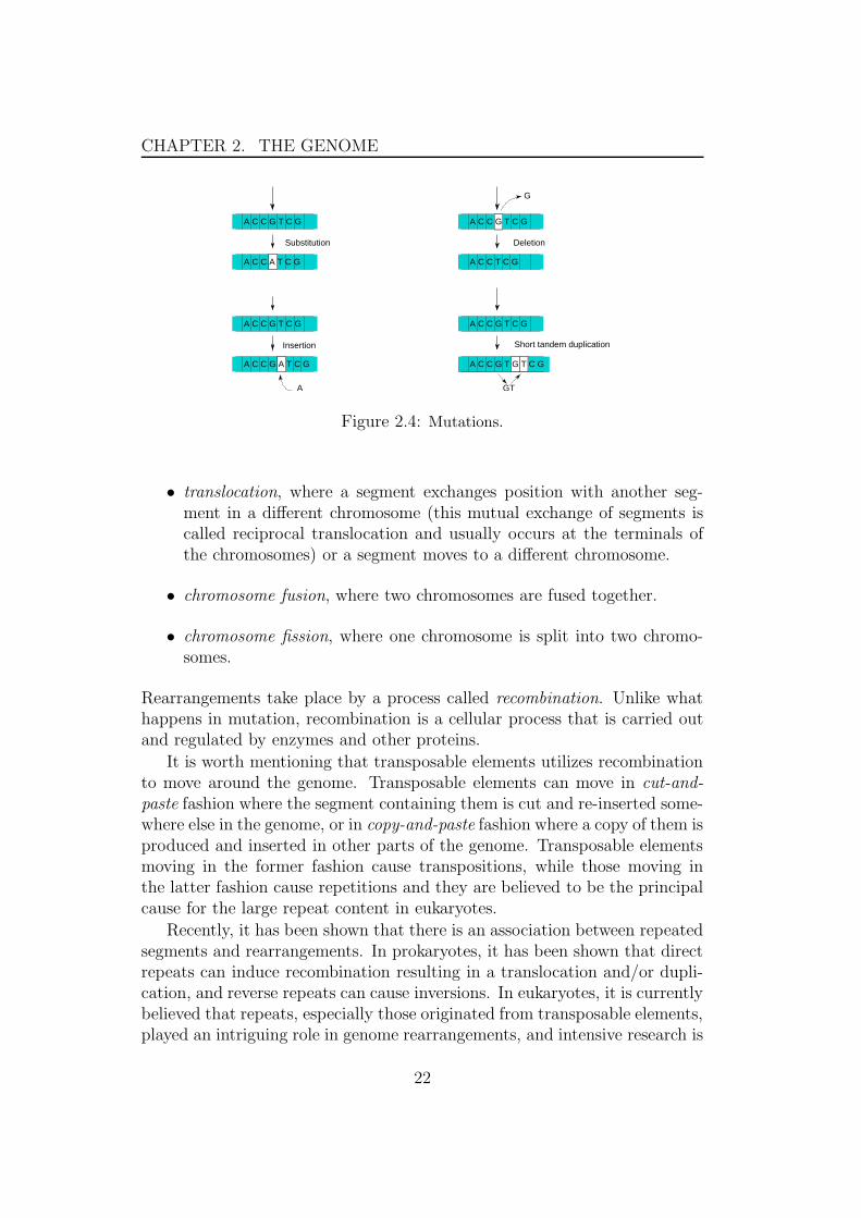
A mutation is a small change in the nucleotide sequence of a DNAmolecule. There are several kinds of mutations:
• substitution, where one nucleotide is replaced with one another.
• insertion, where one or few nucleotides are inserted.
• deletion, where one or few nucleotides are deleted.
• short tandem duplication, where one or few nucleotides are duplicated.The mechanism responsible for short tandem duplications is calledreplication slippage, and is believed to be responsible for the evolutionof microsatellites.
Mutations take place because of errors during the replication of DNA oras a result of external effects such as chemicals and radiation. Figure 2.4shows examples of these kinds of mutations.
A rearrangement changes large segments of the DNA molecule. Thereare several kinds of rearrangement events (see Figure 2.5):
• duplication, where a segment of the genome is duplicated.
• segmental deletion, where a part of the genome is deleted.
• segmental insertion, where a DNA segment is inserted in the genome.
• transposition, where a segment of a genome moves to another place inthe same chromosome.
21
CHAPTER 2. THE GENOME
A C C G T C G
A C C A T C G
A C C G A T C G
A
Substitution
Insertion
A C C G T C G A C C G T C G
A C C G T G T C G
A C C T C G
GT
Deletion
Short tandem duplication
G
A C C G T C G
Figure 2.4: Mutations.
• translocation, where a segment exchanges position with another seg-ment in a different chromosome (this mutual exchange of segments iscalled reciprocal translocation and usually occurs at the terminals ofthe chromosomes) or a segment moves to a different chromosome.
• chromosome fusion, where two chromosomes are fused together.
• chromosome fission, where one chromosome is split into two chromo-somes.
Rearrangements take place by a process called recombination. Unlike whathappens in mutation, recombination is a cellular process that is carried outand regulated by enzymes and other proteins.
It is worth mentioning that transposable elements utilizes recombinationto move around the genome. Transposable elements can move in cut-and-paste fashion where the segment containing them is cut and re-inserted some-where else in the genome, or in copy-and-paste fashion where a copy of them isproduced and inserted in other parts of the genome. Transposable elementsmoving in the former fashion cause transpositions, while those moving inthe latter fashion cause repetitions and they are believed to be the principalcause for the large repeat content in eukaryotes.
Recently, it has been shown that there is an association between repeatedsegments and rearrangements. In prokaryotes, it has been shown that directrepeats can induce recombination resulting in a translocation and/or dupli-cation, and reverse repeats can cause inversions. In eukaryotes, it is currentlybelieved that repeats, especially those originated from transposable elements,played an intriguing role in genome rearrangements, and intensive research is
22

CHAPTER 2. THE GENOME
Duplication
Deletion Insertion Inversion
TranspositionReciprocal Translocation
Figure 2.5: Rearrangement events. Chromosome fusion and fission are not shown.
ongoing. Of course, these rearrangements can be observed only by comparinggenomes of organisms from the same or different species.
2.5 Comparative genomics and perspectives
Sequencing a genome is not an ultimate in itself. A major task, however, is tounderstand the genomic sequence. For some time, scientists thought that thegenomic sequence of an organism would directly present a complete pictureof its biological system. However, the genome sequences have revealed howextreme the gap between our thought and reality is. Of about 4300 genesof the most intensively studied bacterium E. coli, for example, about 38% ofthe genes (reading frames) remained of unknown function. For the humangenome, the exact number of genes is still unknown, and 50% of the locatedgenes are of unknown function. To close this gap, it became clear that manygenomes of different organisms have to be sequenced and compared to eachother. Computational comparative genomics holds much promise in thisrespect because it identifies the regions of similarity and difference amongthe sequences. In the remaining part of this section, we point out some ofits current applications and some future perspectives.
The first step when sequencing a genome is to identify sequence features,such as G+C content of its regions, and to segment the genome into its
23

CHAPTER 2. THE GENOME
structural units, such as genes, repeats, and regulatory elements. Then oneattempts to assign a function to each structural unit and tries to infer itsorigin. The first step is known as genome annotation, while the second isknown as functional genomics. Comparative genomics is a powerful tech-nique for both genome annotation and functional genomics. If one comparesgenomes of two related organisms and a segment is identified, for example,as an exon in one sequence, then a similar segment in the other genome isa potential exon as well. Because similar sequences are very likely to havethe same function, it implies that if the function of a segment is known inone genome, then it can be assigned, with a high degree of certainty, to thesimilar segment in the other. That is, this comparison not only speeds up an-notating the new genomes, but also enables to assign functions to their DNAsegments. To take one example, 46% of the 6200 yeast genes have sequencesimilarity to predicted human genes. This suggests that these proteins arerequired for “housekeeping” functions, such as metabolism, and the genesexisting in other organisms but not in the yeast are hypothesized to be thosethat distinguish the unicellular life form from the multi-cellular one.
For eukaryotic genomes, comparative genomics is expected to put forwardan explanation to the complicated gene structure and the existence of largeintergenic regions. The rationale is that coding regions of closely relatedorganisms are relatively well preserved, while non-coding regions tend to showvarying degrees of conservation (occurrence in different genomes). Therefore,the exons can be located with high precision, and the function and originof such non-coding regions can be revealed by tracing them in genomes ofdifferent organisms.
For prokaryotic genomes, identifying the genomic differences between dif-ferent bacteria, can unveil the strain-specific sequences responsible for givingeach bacteria its own traits. If a certain strain of bacterium is, for exam-ple, pathogenic and another is not, then this approach makes it possibleto develop diagnostic probes specific to this strain. Furthermore, it makesit also possible to design drugs acting on the unique targets (DNA or pro-teins) specific to this pathogenic strain. Another application of interest forbiotechnology is to increase the productivity of a certain (micro) organismthat produces a certain substance, e.g., methane. By comparing the genomeof this organism to others which are deprived of this feature, one can identifythe genes and the regulatory elements responsible for this unique process.Then these specific segments and genes can be genetically processed to in-crease the productivity of the organism.
For human health, hypothesized disease-related genes and segments inthe human genome can be mapped to the corresponding ones in genomes ofother organisms, where they can be tested and genetically manipulated. For
24

CHAPTER 2. THE GENOME
example, about 50% of the human disease-related genes identified so far werefound to be conserved in Drosophila. Subsequently, the Drosophila geneticshas focused on these candidate genes to understand their role and to developtreatment of such diseases.
For evolutionary studies, identifying the regions of similarity and differ-ence in two or more genomes is the first step towards understanding themechanisms responsible for rearrangement events and their underlying func-tional and structural constraints. Moreover, it will be interesting to addressquestions such as “what is the minimum genome content?”, i.e., what is theminimum number of genes to have a living cell? For a certain species, one canalso ask: “what is the minimal set of genes necessary to make an organismbelong to this species?”.
25


Chapter 3
Comparative Genomics Tools:A Survey
The last few years have witnessed the emergence of software tools that areable to handle complete genomes. At first glance, it seems that many of thesetools perform the same comparative genomic task, which is roughly referredto as genome alignment. In actuality, most of the tools were developed tocarry out specific tasks, e.g., for detecting exons, for detecting rearrangementevents, or for figuring out single nucleotide changes in different bacterialstrains. For non-experts, each of these tools seems to have developed itsown methodology. However, most of the tools follow the same strategy,but the details are different and usually adapted to the task at hand. Thissituation has motivated us to present a classification scheme for these toolsbased on the underlying computational technique, and to shed light on thebackground application that caused this differentiation. We would like todraw attention to the fact that many of these tools appeared in the time wepublished our work, and some more recent tools actually made use of ourearlier results, especially those concerning the enhanced suffix arrays. Wehope that this part of the thesis will help the reader to have a comprehensiveand comparative overview of the tools developed until now, to make themost of them, and to evaluate our contribution to the problem of comparinggenomic sequences.
This chapter is organized as follows. The next section presents the basicalgorithms of sequence alignment on the character level, and discusses whythese algorithms are not suitable to apply for comparing whole genomes.In Section 3.2, we outline the basic techniques used in software tools forcomparing genomic sequences. From this section, it will be clear that theanchor-based strategy became the state of the art method in comparing ge-nomic sequences. In section 3.3, we focus on this strategy and examine in
27

CHAPTER 3. COMPARATIVE GENOMICS TOOLS: A SURVEY
detail the techniques used in the anchor based strategy. Section 3.4 reviewseach of the current software tools and outlines the underlying algorithms.Sections 3.5 and 3.5.3 handle some issues related to the anchor based strat-egy, namely the choice of the parameters and the multiple genome alignment.Section 3.6 contains a summary of the chapter, the conclusions, and the openproblems.
3.1 Sequence alignment algorithms
As introduced in Chapter 2, there are three types of biological sequences:DNAs, RNAs, and proteins. In computer science terminology, DNA is astring over an alphabet of four characters, namely A, C, G, and T. RNA isa string over an alphabet of four characters: A, C, G, and U. A protein is astring over an alphabet of 20 characters corresponding to the 20 amino acids.Let S[1 . . . n] denote a DNA string of size n characters (nucleotides). Thecomplement string of a DNA string is obtained by replacing every C with G, G
with C, T with A, and A with T; i.e., this replacement follows the base pairingrule. The reverse string of S[1..n] is the string S[n]S[n−1]..S[1]. The reversecomplement of S is the complement string of S[n]S[n − 1]..S[1]. Neitherthe reverse nor the complement string is of interest in molecular biology.The reverse complement, however, is of the same importance as the DNAstring S because it represents the complementary strand of this molecule,where biological information is also encoded. Using the genetic code, anyDNA or RNA sequence that encodes for a protein can be transformed to thecorresponding sequence of amino acids.
Biological sequence comparison became a known practice since the emer-gence of biological sequence databases. The first databases contained shortsequences, such as genes, proteins, and RNAs. There were technical as wellas biological needs that necessitated sequence comparison. The technicalneed was to avoid redundancy in the database, and the biological need wasto infer the structure and function of new sequences by comparing them tothose that already existed in the database. For example, two genes belong tothe same gene family if they have sufficiently similar sequences. (Recall thedefinition of gene families from Subsection 2.2.3.) This suggests that thesetwo genes probably have a similar function. Furthermore, two similar genesare very likely to be evolved from a common ancestor, and the degree of sim-ilarity can indicate how long ago the two genes, and the organisms includingthem, diverged.
At that time, two or multiple such short sequences were compared on thecharacter level (nucleotides in case of DNA/RNA and amino acids in case of
28
CHAPTER 3. COMPARATIVE GENOMICS TOOLS: A SURVEY
proteins), and the result was delivered in terms of
1. replacements, where characters in one sequence are replaced by othercharacters in the other sequence. If two characters replacing each otherare identical, then they are called a match. Otherwise, they are calleda mismatch.
2. indels, where characters are inserted/deleted in either sequence. (Adeletion in one sequence is an insertion in the other.)
In computer science terminology, character matches, mismatches, dele-tions, insertions are referred to as edit operations, and in biology they repre-sent the mutation events presented in Section 2.4.
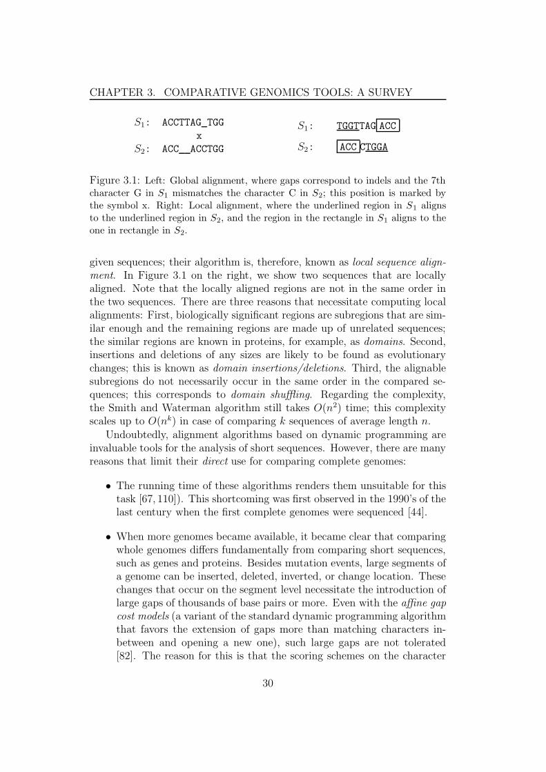
Computer scientists introduced sequence alignment algorithms to effi-ciently compare biological sequences in terms of these edit operations. If twosequences are pre-known to be similar, then global sequence alignment is theprocedure in use. Global alignment of two sequences is a series of successiveedit operations progressing from the start of the sequences until their ends.This alignment can be represented by writing the sequences on two lines onthe page, with replaced characters (matches/mismatches) placed in the samecolumn and inserted/deleted characters placed next to a gap. In Figure 3.1(left), we show an example of aligning the two sequences ACCTTAGTGG andACCACCTGG. From left to right, the series of edit operations is three matchesof ACC, two insertions (deletions) of TT, a match of A, a mismatch of G/C, adeletion (insertion) of C, and three matches of TGG.
If each of the edit operations has a certain score, then the alignment canbe scored as the summation of the edit operation scores. In the example ofFigure 3.1 (left), if a match scores 1, a mismatch scores 0, and an indel haspenalty of -1, then the score of the alignment is 4. In the literature, theindels penalties are also referred to as gap costs.
Because the number of possible alignments is very large, one is interestedonly in an alignment of highest score, which is referred to as optimal globalalignment. In an optimal alignment, the amount of characters replacing eachother (identical or similar characters) are maximized and the amount of gaps(insertions and deletions) is minimized. In 1970, Needleman and Wunsch[112] introduced a dynamic programming algorithm to find an optimal globalsequence alignment. The time and space complexity of their algorithm isproportional to the product of sequence lengths.
In 1981, Smith and Waterman [127] introduced an essential modificationto the Needleman and Wunch algorithm. Instead of computing an optimalglobal alignment, they computed local alignments of subsequences of the
29
CHAPTER 3. COMPARATIVE GENOMICS TOOLS: A SURVEY
S1: ACCTTAG TGG
x
S2: ACC ACCTGG
S1: TGGTTAG ACC
S2: ACC CTGGA
Figure 3.1: Left: Global alignment, where gaps correspond to indels and the 7thcharacter G in S1 mismatches the character C in S2; this position is marked bythe symbol x. Right: Local alignment, where the underlined region in S1 alignsto the underlined region in S2, and the region in the rectangle in S1 aligns to theone in rectangle in S2.
given sequences; their algorithm is, therefore, known as local sequence align-ment. In Figure 3.1 on the right, we show two sequences that are locallyaligned. Note that the locally aligned regions are not in the same order inthe two sequences. There are three reasons that necessitate computing localalignments: First, biologically significant regions are subregions that are sim-ilar enough and the remaining regions are made up of unrelated sequences;the similar regions are known in proteins, for example, as domains. Second,insertions and deletions of any sizes are likely to be found as evolutionarychanges; this is known as domain insertions/deletions. Third, the alignablesubregions do not necessarily occur in the same order in the compared se-quences; this corresponds to domain shuffling. Regarding the complexity,the Smith and Waterman algorithm still takes O(n2) time; this complexityscales up to O(nk) in case of comparing k sequences of average length n.
Undoubtedly, alignment algorithms based on dynamic programming areinvaluable tools for the analysis of short sequences. However, there are manyreasons that limit their direct use for comparing complete genomes:
• The running time of these algorithms renders them unsuitable for thistask [67, 110]). This shortcoming was first observed in the 1990’s of thelast century when the first complete genomes were sequenced [44].
• When more genomes became available, it became clear that comparingwhole genomes differs fundamentally from comparing short sequences,such as genes and proteins. Besides mutation events, large segments ofa genome can be inserted, deleted, inverted, or change location. Thesechanges that occur on the segment level necessitate the introduction oflarge gaps of thousands of base pairs or more. Even with the affine gapcost models (a variant of the standard dynamic programming algorithmthat favors the extension of gaps more than matching characters in-between and opening a new one), such large gaps are not tolerated[82]. The reason for this is that the scoring schemes on the character
30
CHAPTER 3. COMPARATIVE GENOMICS TOOLS: A SURVEY
level imply that long gaps are less likely to occur than short gaps. Thisis of course true for short related sequences, but it is far from realityfor genomic sequences, in which longer gaps are often observed [82].In other words, such gap models cannot perfectly prevent noisy regions(regions where characters match by chance) from interrupting relativelylong gap.
• Another consequence of the large segmental insertions/deletions is thatconserved regions, such as exons, can be relatively short and flanked byunrelated long sequences. A standard dynamic programming algorithmon the character level can easily overlook this homology in favor ofintroducing a larger gap, which is particularly true if the algorithmemploys an affine gap cost model [80].
To sum up, besides their infeasible running time, standard dynamic pro-gramming algorithms cannot accommodate large gaps, and if they attemptto overcome this obstacle, by using extreme parameters of the gap models,they overlook short homologies.
All these limitations of the direct application of sequence alignment algo-rithms motivated computer scientists to develop other methods for comparingwhole genomes. In the remaining part of this chapter, we survey and reviewthese methods. Moreover, we present a classification scheme of such methodsbased on the underlying computational technique.
3.2 Classification scheme of the methods
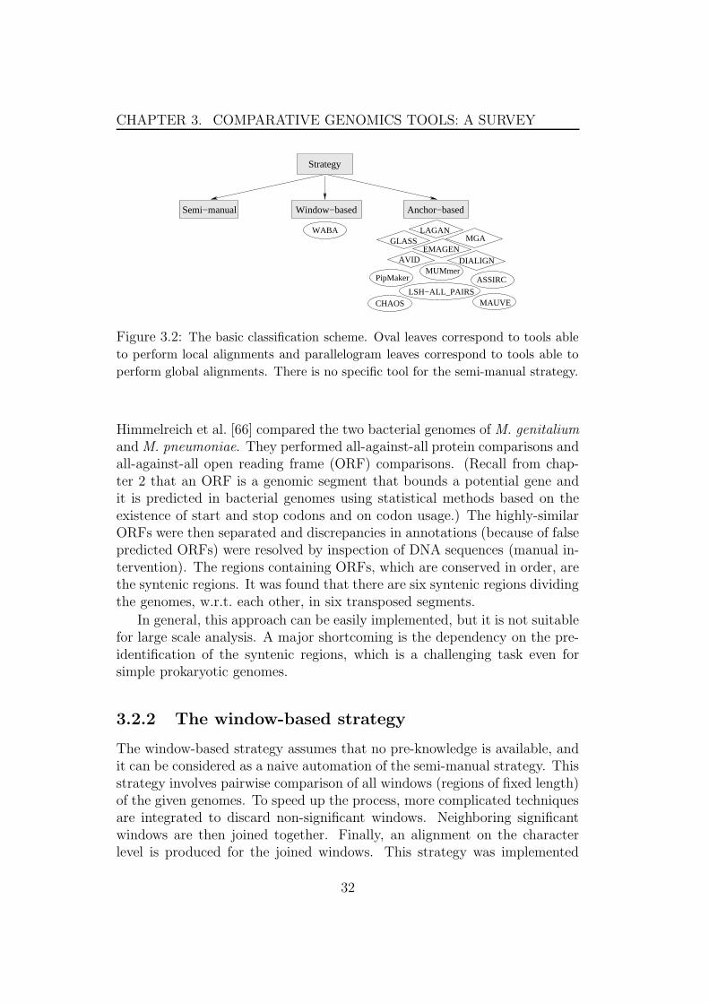
To date, there are three strategies for comparing complete genomes: semi-manual, window-based, and anchor-based. Figure 3.2 shows the three strate-gies along with all tools that follow them.
3.2.1 The semi-manual strategy
In the semi-manual strategy, some knowledge of the genome structure is re-quired. This knowledge is basically information about the syntenic regions(conserved regions in the same order) of the compared genomes. Syntenicregions between genomes can be deduced by identifying specific markers orlocations of known or predicted genes. Once these regions have been iden-tified, the syntenic sequences and the flanking regions are separated andaligned using standard dynamic programming, or other faster heuristic-basedprograms, such as FASTA [116] or BLAST [12]. This method was the firstto be used for comparing complete genomes. To cite one example, in 1997
31
CHAPTER 3. COMPARATIVE GENOMICS TOOLS: A SURVEY
LSH−ALL_PAIRS
Anchor−basedSemi−manual Window−based
Strategy
WABA
CHAOS
GLASS
AVID
PipMakerMUMmer
DIALIGN
ASSIRC
MAUVE
LAGAN
EMAGENMGA
Figure 3.2: The basic classification scheme. Oval leaves correspond to tools able
to perform local alignments and parallelogram leaves correspond to tools able to
perform global alignments. There is no specific tool for the semi-manual strategy.
Himmelreich et al. [66] compared the two bacterial genomes of M. genitaliumand M. pneumoniae. They performed all-against-all protein comparisons andall-against-all open reading frame (ORF) comparisons. (Recall from chap-ter 2 that an ORF is a genomic segment that bounds a potential gene andit is predicted in bacterial genomes using statistical methods based on theexistence of start and stop codons and on codon usage.) The highly-similarORFs were then separated and discrepancies in annotations (because of falsepredicted ORFs) were resolved by inspection of DNA sequences (manual in-tervention). The regions containing ORFs, which are conserved in order, arethe syntenic regions. It was found that there are six syntenic regions dividingthe genomes, w.r.t. each other, in six transposed segments.
In general, this approach can be easily implemented, but it is not suitablefor large scale analysis. A major shortcoming is the dependency on the pre-identification of the syntenic regions, which is a challenging task even forsimple prokaryotic genomes.
3.2.2 The window-based strategy
The window-based strategy assumes that no pre-knowledge is available, andit can be considered as a naive automation of the semi-manual strategy. Thisstrategy involves pairwise comparison of all windows (regions of fixed length)of the given genomes. To speed up the process, more complicated techniquesare integrated to discard non-significant windows. Neighboring significantwindows are then joined together. Finally, an alignment on the characterlevel is produced for the joined windows. This strategy was implemented
32

CHAPTER 3. COMPARATIVE GENOMICS TOOLS: A SURVEY
in a software tool called WABA [82] that was used for the comparison of8 million bp of the C. briggsae genome against the 97 million bp C.elegansgenome [82]. The major drawback of this approach is the running time,which is as high as the product of genome lengths.
3.2.3 The anchor-based strategy
The anchor based strategy is composed of three phases:
1. Generating a set of fragments (regions of similarity) among the givengenomes.
2. Finding certain sets of fragments, called the anchors, identifying syn-tenic regions.
3. Applying a standard dynamic programming technique in the regionswithin and surrounding the anchors.
The anchor-based strategy has become the strategy of choice for com-paring complete genomes. This is because of (1) its efficiency, running insubquaratic time, and (2) its ability to overcome the challenges facing thetraditional sequence alignment algorithms. Specifically, the hierarchal struc-ture of this strategy allows to detect short homologies, by careful generationof the fragments, and long gaps are naturally introduced through the secondstep of identifying the anchors. These advantages will be clear as we moveforward through this chapter.
The tools that are based on the anchor based strategy can be classifiedaccording to the computational techniques used in the first and second phase.In the following section, we will survey and review these techniques in detail.
3.3 Techniques in the anchor-based strategy
3.3.1 Fragment generation techniques
Notions
Let Si[1 . . . ni], 1 ≤ i ≤ k, denote a string of length |Si| = ni. In ourapplication, Si is the DNA sequence of a genome. Si[li . . . hi] is the substringof Si starting at position li and ending at position hi. A fragment defines asimilar region occurring in the given genomes. This region is specified by thesubstrings S1[l1 . . . h1], S2[l2 . . . h2], . . . , Sk[lk . . . hk], where 1 ≤ li < hi ≤ ni
and 1 ≤ i ≤ k. If S1[l1 . . . h1] = S2[l2 . . . h2] = . . . = Sk[lk . . . hk], i.e., the
33
CHAPTER 3. COMPARATIVE GENOMICS TOOLS: A SURVEY
substrings are identical, then the fragment is called exact and it is of thetype multiple exact match. If the equality S1[l1 − 1] = · · · = Sk[lk − 1] doesnot hold, then the multiple exact match is called left maximal, i.e., it cannotextend to the left in the given genomes. Similarly, if the equality S1[h1 +1] =· · · = Sk[hk + 1] does not hold, then the multiple exact match is calledright maximal. The multiple exact match is called maximal, abbreviatedby multiMEM , if it is both left and right maximal. If we speak of twosequences, then multiMEMs are referred to as maximal exact matches, andthey are abbreviated by MEMs. If the substrings composing a fragmentare restricted to be unique in the respective genomes, then they compose amaximal multiple unique match, abbreviated by multiMUM . If we speak oftwo sequences, then multiMUMs are referred to as maximal unique matches,and they are abbreviated by MUMs. multiMEMs and multiMUMs will beaddressed in more detail in Chapter 4. If the length of the substrings is fixedto a certain length, i.e., hi − li = k, then the substrings are called k-mersand they compose a fragment of exact k letters. Unless stated otherwise, wewill use the word k-mers to mean, for short, fragments of size k. (Fragmentsof exact k-mers are known in the field of string processing as q-grams, whereq = k.) If mismatches, deletions, or insertions of characters are allowed inthe substrings, i.e., S1[l1 . . . h1] ≈ S2[l2 . . . h2] ≈ · · · ≈ Sk[lk . . . hk], then wespeak of a non-exact fragment. If the length of the substrings composing thenon-exact fragments is fixed to a certain length, i.e., hi − li = k, then we callthe fragments non exact k-mers. Note that if the substrings composing afragment are of different lengths, then an alignment of these substrings willcontain character indels. Later in this chapter, we will discuss the advantagesand disadvantages of using each kind of fragments for comparing genomicsequences.
In general, there are several techniques for computing fragments. How-ever, we limit ourselves to the techniques used in comparative genomics.These techniques include exhaustive enumeration, hashing, automata (tries),the usage of the suffix trees, and the usage of the enhanced suffix arrays. Fig-ure 3.3 shows the different techniques and the tools implementing them.
Exhaustive enumeration
This technique is one of the oldest techniques used to compute fragments.It is used only in the software tool DIALIGN [106, 107] to compare proteinand relatively short DNA sequences. The basic idea is that fragments arethe result of cross-products between all substrings of the genomes involved.In a genome of average size n, we have O(n2) substrings. Thus, for twogenomes, there are O(n4) fragments. To reduce the number of fragments,
34

CHAPTER 3. COMPARATIVE GENOMICS TOOLS: A SURVEY
Fragment Generation
Suffix Tree Enhanced Suffix ArrayExhaustive Hashing Automata/Trie
CHAOSWABA
BLASTZGLASS
MUMmerAVID
MGADIALIGN
Mauve
ASSIRC EMAGEN
LSH−ALL_PAIRS
Figure 3.3: Fragment generation techniques and the tools using it.
the cross products can be limited to substrings of the same length. Thisreduces the number of fragments to O(n3). To further reduce this number,only substrings of maximum length l are taken into account. This makesthe number O(n2l). Even with the O(n2l) fragments, this technique is stillinfeasible for comparing whole genomes.
Hashing techniques
In the hashing technique, a hash table is constructed to store the locationsof all substrings of length k in one of the genomes. The hash table can be di-rectly used to compute exact k-mers, and non-exact k-mers of two sequences.
For computing exact k-mers, the hash-table is constructed so that itsentries contain the positions of all substrings of length k of one genome. Thehashing function for a substring S[l..l + k − 1] is
x =l+k−1∑
i=l
|Σ|i−lT (S[i])
where x is an integer value representing an index of the hash table, |Σ| is thealphabet size, and T (S[i]) is a bijective function that maps each characterin the alphabet to a number in the range [0 . . . |Σ| − 1] 1. Then the secondgenome is streamed against this table to locate the k-mers. More precisely,each substring of length k of the second genome is matched against this table.
Constructing the hash table for constant k takes linear time, specifi-cally O(n1), where n1 is the length of the first genome. Deciding whether aquery substring exists in the table takes constant time and enumerating thematches, if any, takes time proportional to their number. Because there areO(n2) substrings in the second genome, which is of length n2, reporting all
1This table is a direct address table, but it is usually referred to as hash table inbioinformatics literature.
35
CHAPTER 3. COMPARATIVE GENOMICS TOOLS: A SURVEY
the z k-mers takes O(n2 + z) time. Therefore, the total time complexity isO(n1 +n2 + z). Because the space consumption increases exponentially withk, k is usually chosen to be between 7 and 20. For whole genomes, it is ex-pected that almost all substrings of length k occur; i.e., no entry of the hashtable would be empty. As we shall see in Section 3.4, the hashing technique,because of its simplicity, is widely used in software tools such as WABA [82],BLASTZ [124] (PipMaker [125]), BLAT [81], ASSIRC [136], GLASS [19],and LSH-ALL-PAIRS [34].
The hashing-technique can also be used to compute non-exact k-mers.There are two kinds of non-exact k-mers: The first restricts the allowedmismatches to fixed positions of the k-mer, but the second does not. Theformer kind of k-mers can be specified by a certain pattern or mask of onesand zeros. For example, it can be required to report all 8-mers such thatthe third and sixth characters are not necessary identical (do not care) inboth genomes. The respective mask is 11011011, where the ones correspondto the locations of the identical characters, and the zeros correspond to thelocations where mismatches are allowed.
To find all k-mers according to a pre-determined mask, the hash tableis constructed so that its entries contain positions of substrings of the firstsequence S1, but the indices encode subsequences of these substrings. For asubstring of length k, the respective subsequence is made up of the d′ < kcharacters that match the 1s of the mask. Let us take one example, supposethat S1 contains the substring w = aabc at position l1. Assuming thatk = 4 and the mask is 1101, then the index corresponding to w is computedaccording to the subsequence aac, and the entry next to it stores l1. Afterconstructing the hash-table, the second genome is streamed against it asfollows. For each substring of length k of the second genome, one constructsthe substring β, |β| = d′, containing the subsequence of characters that fitthe 1s of the mask. For example, for a substring aagc at position l2, β = aac.If β is used as a query against the above hash table, which has an entry forw, then the match (l1, l2, k) is obtained.
The hashing technique was used first in PatternHunter [99] to locatenon-exact k-mers according to a certain mask, and it was employed later ina recent version of BLASTZ [124].
To find non-exact k-mers so that mismatches are allowed at any positions,the streaming phase of the second genome has to be modified. Assume thatit is required to generate non-exact k-mers such that at most one mismatchis allowed at any position of the k-mer. For each substring of the secondgenome, every character is replaced by every other character in the alphabetone at a time. Then the resulting substring is queried against the hash table.In total, there are k(|Σ| − 1) +1 queries launched for each substring: one for
36
CHAPTER 3. COMPARATIVE GENOMICS TOOLS: A SURVEY
the original substring and k(|Σ−1|) for the replaced characters. If more thanone mismatch is allowed in the same k-mer, then the queries are composedby taking all combinations of all replaced characters at every two positionsof each substring.
Before moving to another fragment generation technique, it is worth men-tioning that the hashing technique was used to compute multiMEMs [96],when suffix trees (presented in Chapter 4) were not so popular in bioinfor-matics. The idea was as follows. First the compared sequences are concate-nated in a single sequence. Then a hash table is constructed for all substringsof length k of the resulting sequence. The identical substrings (at the samehash table entry) are checked for left maximality, i.e., the characters preceed-ing them are examined. If they are preceeded by different characters, thenthey are divided into groups according to the preceeding characters. Oth-erwise, they are discarded because they are contained in longer substrings.For each group the substrings are extended to the right until the charactersto the right are different. Then they are divided into subgroups according tothe succeeding characters. A cross-product is then performed between sub-groups of different groups to report the multiMEMs, if their length is higherthan a certain threshold. The left and right extension steps are recursivelyapplied for substrings in the same groups. Interestingly, a similar approachwas recently used in the software tool Mauve [43] to compute multiMUMs.
Automata and tries
Automata can be used to compute exact and non-exact k-mers instead ofconstructing a hash-table. Aho and Corasick [10] showed how to constructa deterministic finite automata for a set of keys (words). The target was toimprove online string matching for bibliographic search. For a genomic se-quence, the keys of the automaton are the set of its substrings. The locationswhere these substrings occur in the sequence can be attached to the nodesof success of the automaton. Figure 3.4 shows an example of an automatonconstructed to compute 4-mers for the string acctca. The string has the threekeys acct, cctc, and ctca. For computing k-mers, each substring of length kof the other sequence is matched against this automaton. As we shall see inSection 3.4, a modified version of this data structure is used in the softwaretool CHAOS [33].
It is interesting to see that this automaton is nothing but a pruned non-compact suffix tree. As will be explained in the next chapter, a non-compactsuffix tree, known as trie, has the edge labels explicitly stored with the tree,and for each label there is an edge. (As a consequence not all the nodesof the tree are branching.) Because the space consumption of a trie grows
37
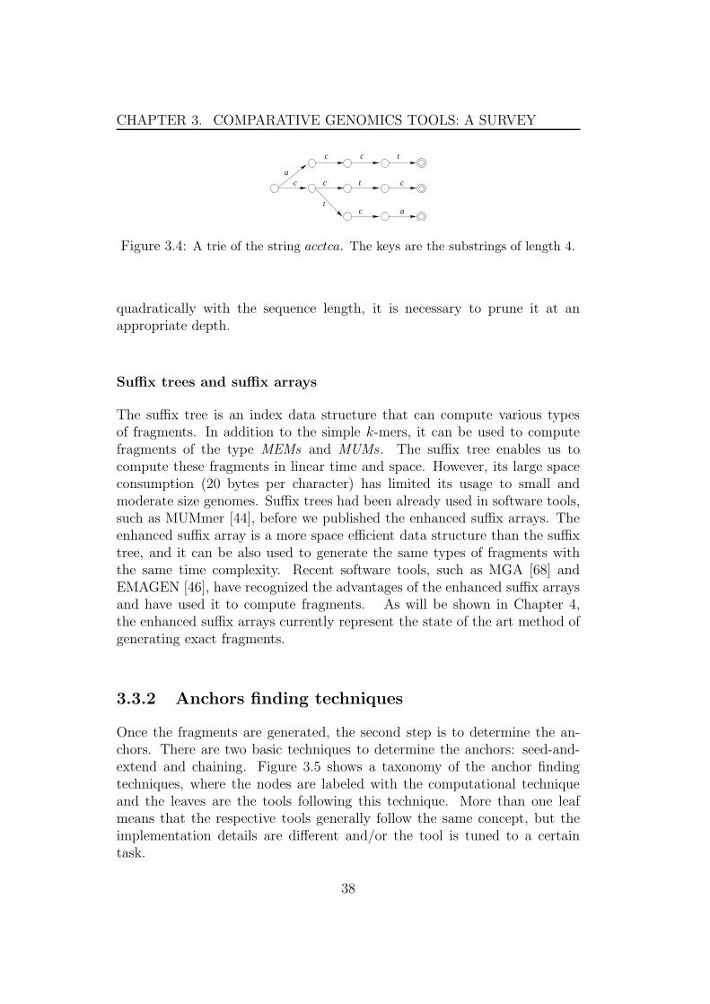
CHAPTER 3. COMPARATIVE GENOMICS TOOLS: A SURVEY
c
a
c
c c t c
t
tc a
Figure 3.4: A trie of the string acctca. The keys are the substrings of length 4.
quadratically with the sequence length, it is necessary to prune it at anappropriate depth.
Suffix trees and suffix arrays
The suffix tree is an index data structure that can compute various typesof fragments. In addition to the simple k-mers, it can be used to computefragments of the type MEMs and MUMs. The suffix tree enables us tocompute these fragments in linear time and space. However, its large spaceconsumption (20 bytes per character) has limited its usage to small andmoderate size genomes. Suffix trees had been already used in software tools,such as MUMmer [44], before we published the enhanced suffix arrays. Theenhanced suffix array is a more space efficient data structure than the suffixtree, and it can be also used to generate the same types of fragments withthe same time complexity. Recent software tools, such as MGA [68] andEMAGEN [46], have recognized the advantages of the enhanced suffix arraysand have used it to compute fragments. As will be shown in Chapter 4,the enhanced suffix arrays currently represent the state of the art method ofgenerating exact fragments.
3.3.2 Anchors finding techniques
Once the fragments are generated, the second step is to determine the an-chors. There are two basic techniques to determine the anchors: seed-and-extend and chaining. Figure 3.5 shows a taxonomy of the anchor findingtechniques, where the nodes are labeled with the computational techniqueand the leaves are the tools following this technique. More than one leafmeans that the respective tools generally follow the same concept, but theimplementation details are different and/or the tool is tuned to a certaintask.
38
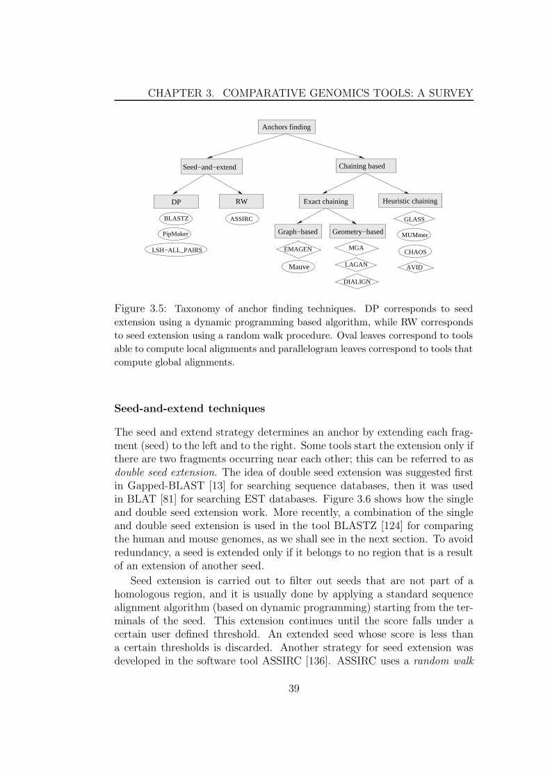
CHAPTER 3. COMPARATIVE GENOMICS TOOLS: A SURVEY
Anchors finding
PipMaker
BLASTZ
EMAGEN
Mauve
Exact chaining Heuristic chaining
Seed−and−extend
ASSIRC GLASS
Geometry−basedGraph−based
Chaining based
LAGAN
LSH−ALL_PAIRS
DIALIGN
AVID
CHAOS
MUMmer
DP RW
MGA
Figure 3.5: Taxonomy of anchor finding techniques. DP corresponds to seed
extension using a dynamic programming based algorithm, while RW corresponds
to seed extension using a random walk procedure. Oval leaves correspond to tools
able to compute local alignments and parallelogram leaves correspond to tools that
compute global alignments.
Seed-and-extend techniques
The seed and extend strategy determines an anchor by extending each frag-ment (seed) to the left and to the right. Some tools start the extension only ifthere are two fragments occurring near each other; this can be referred to asdouble seed extension. The idea of double seed extension was suggested firstin Gapped-BLAST [13] for searching sequence databases, then it was usedin BLAT [81] for searching EST databases. Figure 3.6 shows how the singleand double seed extension work. More recently, a combination of the singleand double seed extension is used in the tool BLASTZ [124] for comparingthe human and mouse genomes, as we shall see in the next section. To avoidredundancy, a seed is extended only if it belongs to no region that is a resultof an extension of another seed.
Seed extension is carried out to filter out seeds that are not part of ahomologous region, and it is usually done by applying a standard sequencealignment algorithm (based on dynamic programming) starting from the ter-minals of the seed. This extension continues until the score falls under acertain user defined threshold. An extended seed whose score is less thana certain thresholds is discarded. Another strategy for seed extension wasdeveloped in the software tool ASSIRC [136]. ASSIRC uses a random walk
39
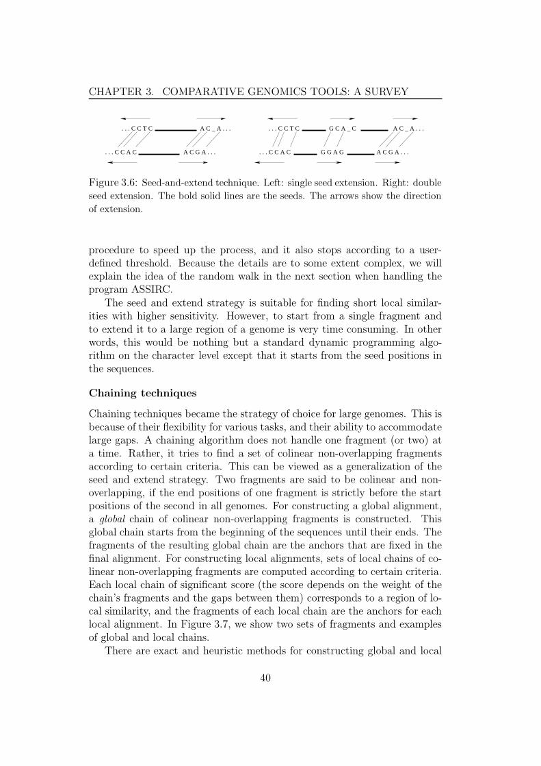
CHAPTER 3. COMPARATIVE GENOMICS TOOLS: A SURVEY
A C _ A . . .
A C G A . . .
G C A _ C
G G A GA C G A . . .
A C _ A . . .. . . C C T C
. . . C C A C
. . . C C T C
. . . C C A C
Figure 3.6: Seed-and-extend technique. Left: single seed extension. Right: double
seed extension. The bold solid lines are the seeds. The arrows show the direction
of extension.
procedure to speed up the process, and it also stops according to a user-defined threshold. Because the details are to some extent complex, we willexplain the idea of the random walk in the next section when handling theprogram ASSIRC.
The seed and extend strategy is suitable for finding short local similar-ities with higher sensitivity. However, to start from a single fragment andto extend it to a large region of a genome is very time consuming. In otherwords, this would be nothing but a standard dynamic programming algo-rithm on the character level except that it starts from the seed positions inthe sequences.
Chaining techniques
Chaining techniques became the strategy of choice for large genomes. This isbecause of their flexibility for various tasks, and their ability to accommodatelarge gaps. A chaining algorithm does not handle one fragment (or two) ata time. Rather, it tries to find a set of colinear non-overlapping fragmentsaccording to certain criteria. This can be viewed as a generalization of theseed and extend strategy. Two fragments are said to be colinear and non-overlapping, if the end positions of one fragment is strictly before the startpositions of the second in all genomes. For constructing a global alignment,a global chain of colinear non-overlapping fragments is constructed. Thisglobal chain starts from the beginning of the sequences until their ends. Thefragments of the resulting global chain are the anchors that are fixed in thefinal alignment. For constructing local alignments, sets of local chains of co-linear non-overlapping fragments are computed according to certain criteria.Each local chain of significant score (the score depends on the weight of thechain’s fragments and the gaps between them) corresponds to a region of lo-cal similarity, and the fragments of each local chain are the anchors for eachlocal alignment. In Figure 3.7, we show two sets of fragments and examplesof global and local chains.
There are exact and heuristic methods for constructing global and local
40

CHAPTER 3. COMPARATIVE GENOMICS TOOLS: A SURVEY
(a)
4 75
5 72 3
(b)
1
2
4 5
6
7 8
9
3
1 4 67 8
1
2
1g
g g2
1g
2 3 6
Figure 3.7: Left: global chaining. The global chain is composed of the fragments
2, 3, 5, and 7. Right: local chaining. There are two local chains. The first is
composed of the three fragments 1, 4, and 6, and the second is composed of the
two fragments 7, and 8.
chains. In the exact methods, the chaining algorithm finds optimal chainsthat maximize (minimize) a certain objective function. In the heuristic meth-ods, the optimality of the chains is not guaranteed.
The exact chaining algorithms can be further sub-divided into two groupsaccording to the underlying computational paradigm/model: graph basedand geometric based. In the former paradigm, a directed acyclic graph isconstructed so that the fragments are the nodes and the edges are addedaccording to the colinearity and non-overlapping constraint. The edges areweighted, for example, by the length or statistical significance of the frag-ments. The optimal solution is then reduced to finding an optimal path inthis graph. This graph based solution, will be handled in detail in Chapter5. Although this graph based solution is flexible, it requires O(m2) time tofind an optimal solution, where m is the number of fragments. This can be asevere drawback if a large number of fragments has to be chained. Geometricbased algorithms make use of the geometric nature of the problem. They aresubquadratic and can handle a large number of fragments efficiently. The ge-ometric based algorithms are the basic topic of Chapter 5, where we presentour chaining algorithms.
The heuristic methods had been used in the tools before we published ourchaining algorithms. Because the heuristics in use differ significantly fromtool to tool, each one will be addressed when handling the respective tool.We think that there are a number of reasons why these heuristics were de-veloped. First, the exact solutions known at that time were based either ongraph formulation or on a sophisticated technique known as sparse dynamic
41
CHAPTER 3. COMPARATIVE GENOMICS TOOLS: A SURVEY
programming [50]. The former is quadratic in the number of fragments, andthe latter is very complicated to implement; although it has sub-quadratictime complexity. Second, the exact solutions were already available for gen-erating only global chains and it was not clear how to incorporate othervariations that are necessary for whole genome comparisons. These varia-tions include, among others, gap constraints, local chaining, and fragmentsof draft genomes. In Chapter 5, we will present our chaining algorithms,which are geometric based but not as complicated as the sparse dynamicprogramming algorithm of [50]. We will show also how to include many vari-ations, such as the aforementioned ones, for solving versatile comparativegenomic tasks efficiently.
In Figure 3.5, we show the taxonomy of the chaining techniques. We alsoshow the tools following each technique. Because chaining algorithms formultiple genomes are not used in all tools, this taxonomy takes into accountchaining algorithms for two genomes, i.e., two dimensional chaining.
3.4 The tools
Except for the software tool WABA, all the tools apply the anchor basedstrategy. The software tools are not reviewed in chronological order, butaccording to the relatedness of the underlying techniques.
3.4.1 WABA
WABA is the only tool that was developed using the window based strategy.It was used for the comparison of 8 million bp of the C. briggsae genomeagainst the 97 million bp C.elegans genome [82]. WABA is composed ofthree phases.
In the first phase, the shorter genomic sequence, C. briggsae, is called aquery and the larger one, C.elegans, is called target. The query genome isdivided into overlapping sections, each is of length 2000 bp. Then k-mersare computed between this section and the target genome. An interestingfeature of WABA is the usage of non-exact 8-mers whose mask is 11011011.The rationale behind choosing this mask is that the first and second positionsof codons corresponding to the same amino acid are fairly well preserved,while the third, wobble, position is not. (Recall from Chapter 1 that thegenetic code is redundant, i.e.; multiple codons can correspond to the sameamino acid.) This feature is, of course, important if we compare codingregions of different genomes. WABA computes these 8-mers using a hashingtechnique.
42
CHAPTER 3. COMPARATIVE GENOMICS TOOLS: A SURVEY
In the second phase, windows of length 5000 bp of the target genomeare compared to significant windows of the first phase. A window is consid-ered significant if it contains 8-mers whose number is greater than a certainthreshold. For each significant window, an alignment is computed using analgorithm based on Hidden Markov Models (HMMs). The reason for us-ing HMMs is to make the alignment phase “at least as wobble aware” asthe fragment generation phase. In the third phase, overlapping alignments(windows) are merged into larger alignments.
WABA was the first to consider divergence in the wobble position ofcoding regions, which is important for the application of comparative exonprediction. However, its running time, which is quadratic in the genomesizes, renders it inefficient for comparing whole genomes. For this moderatesize task, WABA took about 12 days (on a Pentium III 450 MHz).
3.4.2 PipMaker and BLASTZ
PipMaker
PipMaker, Percentage Identity Plot Maker, is a web server developed todeliver and visualize local alignments [125]. PipMaker can perform pre-processing on the sequences before aligning them. This includes, amongothers, formatting the input sequences and masking repeats using the pro-gram RepeatMasker [126]. The local alignments themselves are computedusing a program called BLASTZ [124]. For post processing, PipMaker vi-sualizes the output of BLASTZ in many forms. Among these forms is thepercentage identity plot pip, where the percentage of identical characters ineach local alignment is plotted against its position in one of the input se-quences. PipMaker includes other options such as global chaining and singlecoverage for post processing BLASTZ output. These options were added inPipMaker to avoid duplicate matches (each position in one sequence aligns toat most one sequence in the other sequence). Global chaining is appropriatefor regions whose homologous regions are conserved in order, while singlecoverage is appropriate if the conservation in order does not hold. We willexplain both options in detail in Chapter 5. There, we will see that the singlecoverage procedure is nothing but a one dimensional chaining procedure.
PipMaker was recently enhanced with a second server, MultiPipMaker[123], that performs multiple sequence alignment. It constructs the multiplealignment by merging the pairwise alignments between one sequence (“ref-erence sequence”) and each of the other sequences (“secondary sequences”).More specifically, the multiple alignment is produced in two phases: In thefirst phase the reference sequence is aligned individually with each one of
43
CHAPTER 3. COMPARATIVE GENOMICS TOOLS: A SURVEY
the secondary sequences using BLASTZ. The local alignments are furtherprocessed such that each position in the reference sequence aligns with atmost one position in the secondary sequence. Afterwards, the alignments aremerged by building a matrix whose first row is the reference sequence and theremaining rows are the secondary sequences. However, for each secondarysequence the regions that are aligned to the reference sequence are swapped(rearranged) in the row so that they appear according to their occurrence inthe reference sequence.
In the second phase, the above crude multiple alignment is refined, byemploying a strategy developed by Anson and Myers [14]. Briefly, this strat-egy works by realigning each subregion of the multiple alignment. If the scoreof the multiple alignment improves, then the realignment of this subregionis fixed in the final alignment.
In fact, this algorithm computes local alignments among genomes, butw.r.t. a reference sequence. In other words, the procedure makes it possibleto see where each region of the reference sequence aligns to the secondarysequences. After the merging, one can identify the common regions betweenall compared genomes. However, because each position in the reference se-quence aligns with at most one position in a secondary sequence, repeatedsegments in the secondary sequences cannot be represented in the multiplealignment.
BLASTZ
BLASTZ [124] is the main computational engine of PipMaker and MultiP-ipMaker. It is based on the hashing technique for computing fragments andthe seed-and-extend technique for finding the anchors.
The hashing technique of BLASTZ can deliver exact 8-mers and non-exact 19-mers according to the mask 11101100110010101111. This maskwas suggested by Ma et al. [99] to increase the sensitivity when comparingdivergent sequences. To further increase the sensitivity, the authors allow anextra “transition” (mismatch of A/G, G/A, C/T, and T/C) in any of theidentical characters of this mask. These transitions can be taken into accountwhile streaming the second genome against the hash table as follows. Foreach character in a substring of the second genome fitted to a 1 of the mask,a transition is done by toggling A to G, G to A, C to T, and T to C. Then foreach transition the resulting pattern is queried against the hash-table. Thatis, 13 queries are launched for each substring: 1 for the original pattern and12 for the toggled characters.
The extension of seeds is done in two phases: The first phase computesrelatively short local similarities, and it involves applying a standard dynamic
44

CHAPTER 3. COMPARATIVE GENOMICS TOOLS: A SURVEY
programming algorithm to the left and to the right of a seed. The extensionterminates once the score falls under some threshold. Extended seeds thatscore less than a certain threshold are discarded. The second phase attemptsto produce larger local alignments by organizing the extended seeds of thefirst phase. This is done using a double-seed extension procedure as follows.The extended seeds obtained from the first phase are used as seeds. Butthe extension is initiated between each pair of seeds that are separated byless than a certain threshold in both genomes. The extension is done in theregion separating the two seeds using the same procedure of the first phase,but with exact 7-mers as primary seeds.
The usage of non-exact k-mers and the second phase of seed extensionwas not yet implemented in the BLASTZ version published with PipMaker.These modifications were recently suggested and integrated particularly forcomparing the human genome against the recently-finished mouse genome.The authors of BLASTZ wrote: “an alignment program with higher sensi-tivity”. However, the running time of BLASTZ is a major drawback. Asreported by the authors, it takes 481 days of CPU time and a half day ona cluster of 1024 Pentium III CPUs (833 MHz). We think there are somereasons for this: First, the number of k-mers is too large to be handledefficiently; this caused the authors to divide the human genome into 3000overlapping segments (each of 1.01 million bp) and the mouse genome intoone hundred segments (each of about 30 million bp). Second, there are nu-merous long conserved regions between human and mouse genomes. Theextention that starts from a single seed using standard dynamic program-ming, which is quadratic, can proceed all over the entire regions withoutdrop in the score. That is, the running time of the algorithm grows quadrat-ically with the lengths of the conserved regions. Third, testing and extendingall pairs of extended seeds in the second phase then re-joining the dividedsegments of both genomes are also tough tasks.
3.4.3 LSH-ALL-PAIRS
The program LSH-ALL-PAIRS was developed to compute local alignmentsbased on the seed and extend technique [34]. What basically differentiatesthis tool is the usage of non-exact k-mers computed by a randomized algo-rithm.
For every substring s of length k of each input sequence, d indices i1 . . . idare randomly chosen. Then a hash function f(s) = (s[i1], s[i2], . . . , s[id]) iscomputed. All substrings of both sequences are clustered according to thehash function value. All pairs of substrings whose f(s) values are equal andoccur in different sequences are potential k-mers. To avoid false positives,
45

CHAPTER 3. COMPARATIVE GENOMICS TOOLS: A SURVEY
each k-mer is examined before reporting it to see if the substrings composingit are actually different by at most r characters (r, k, and d are user definedparameters).
The extension is done by searching the regions surrounding each k-mer(search range is 500 bp) to find a nearby similar pair separated by the samenumber of characters. This is to fill the region in-between only in terms ofmatches and mismatches, i.e., no gaps are allowed.
Many drawbacks of this approach can be easily identified. The selectionof seeds is randomized so that some seeds, and therefore some significant sim-ilarities, may be missed by chance. The extension step does not allow gaps,which is unsuitable for comparing diverged genomic sequences. Moreover,the number of non-exact k-mers is still too large to handle large genomes.
3.4.4 ASSIRC
ASSIRC was developed to compute local alignments based on the seed andextend technique [136]. The seeds used by ASSIRC are exact k-mers and theextension is based on a random walk procedure.
A random walk plot is a two dimensional plot in which a sequence ofcharacters is represented by a series of displacement vectors. That is, eachcharacter corresponds to a displacement vector with a certain direction andamplitude. For example, character A corresponds to the displacement vector1−→x (amplitude equals 1 and direction equals 0◦); the vector for C is −1−→x ,for T is 1−→y , and for G is −1−→y . In other words, a sequence of characters isa vector obtained by adding all displacement vectors of all characters. Forexample, a sequence AAT yields the vector 2−→x + 1−→y .
Starting from a terminal of a fragment, the walk proceeds in each sequenceindependently but the distance between the two displacement vectors is ex-amined. Once the distance exceeds a certain threshold, the extension stops.This walk is also done for the other terminal of the fragment. Finally, theextended regions are collected and aligned using standard dynamic program-ming. Fragments that occur in an extended region of another fragment arenot processed again.
This algorithm also depends on k-mers, whose number is too large forlarge genomes. Moreover, the random walk procedure is sensitive to mis-matches, and gaps cannot be explicitly handled.
3.4.5 DIALIGN
DIALIGN was one of the first tools that deviated from directly applyingthe standard dynamic programming algorithm for sequence comparison [106,
46
CHAPTER 3. COMPARATIVE GENOMICS TOOLS: A SURVEY
107]. It is also one of the first tools that applied chaining algorithms forprocessing the fragments. In fact, DIALIGN was not designed to speed up thestandard dynamic programming for comparing large sequences. Rather, itwas developed to improve the alignment quality so that the global alignmentis a series of high scoring segments other than a series of edit operations.This feature of DIALIGN is of special importance when aligning sequences,such as proteins, where the most relevant biological information exists indomains.
DIALIGN uses non-exact k-mers as fragments (the authors of DIALIGNcall these fragments “gap-free fragments”.) These fragments are computedin DIALIGN using the exhaustive technique described before. To speed upthe comparison for long sequences, only fragments of user defined maximumlength are generated. This step takes time proportional to the product ofsequence lengths. The score of a fragment is a function in the number ofidentical characters, its length, and the genomic sequence sizes.
For two sequences, DIALIGN finds a global chain of colinear and non-overlapping fragments. The chain is the alignment produced by DIALIGN;keep in mind that the alignment in DIALIGN is a series of fragments. Thisalgorithm chains the fragments while they are generated, but without con-sidering gap costs. Basically, the algorithm works in a way similar to thestandard dynamic algorithm but the score of the chain (alignment) is thesum of fragment scores rather than edit operation scores. The chaining stepis bounded by O(n1 × n2), where n1, n2 are the genome lengths. This algo-rithm is tailored to deal with fragments computed in such exhaustive way.In Chapter 5, we will present a general and more efficient algorithm thatcan chain fragments while being generated. Moreover, we will show how gapcosts can be efficiently incorporated.
DIALIGN can also be used for constructing a global multiple sequencealignment. The underlying algorithm is based on generating all pairwisealignments. Then a greedy algorithm is used to merge these alignments in asingle multiple alignment. This is done by sorting the fragments containedin these pairwise alignments according to their score and according to thedegree of overlap with other fragments. This favors motifs (highly conservedshort regions) occurring in more than two sequences. The sorted fragmentsare inserted one by one in the alignment provided that they are “consistent”(colinear and non-overlapping with other fragments in the alignment). Non-consistent fragments are discarded.
DIALIGN has showed success for comparing short sequences, such asproteins and genes. The major drawback is its running time, which increasesquadratically with the genome lengths. For example, aligning six variolagenomes, each of only about 180 Kbp, did not complete after one week [36].
47
CHAPTER 3. COMPARATIVE GENOMICS TOOLS: A SURVEY
This drawback was also reported in [33]. Moreover, the greedy algorithm forconstructing global sequence alignment is not flexible in the sense that oncea fragment is incorporated in the alignment, it cannot be removed regardlessof any other better combination.
3.4.6 GLASS
GLASS is a global alignment program tuned for finding conserved exonsbetween two sequences [19]. A potential application, therefore, is exon pre-diction by aligning new sequences to already known sequences.
The fragments of GLASS are computed by first locating all exact 20-mers. These exact 20-mers are then extended 12 characters to the left andto the right using standard dynamic programming. Extended 20-mers arethen dealt with as fragments, and those that score less than a user definedthreshold are discarded. GLASS uses a greedy global chaining procedureto determine the anchors: Fragments that are overlapping, or not colinearwith other fragments that are already fixed in the alignment, are discarded.The same procedure is then recursively applied on the regions between theanchors but with shorter k-mers (20, 15, 12, 9, . . . , 5). Finally, the remainingregions are aligned using standard dynamic programming.
This program was specifically developed to align two short regions ofknown synteny to identify the common exons. There are two reasons thatrender it inefficient for whole genome comparison. First, the ad-hoc globalchaining step favors local similarities, which can be acceptable for comparingshort exons but not for computing global alignment. Second, the number ofk-mers is too large to be dealt with efficiently.
Experiments on the space consumption and running time of GLASS canbe found in [28, 36]. Briefly, the authors of [28] have reported that the mea-sured running time of the program on moderate size sequences was muchhigher than that of the “general purpose” alignment programs, and the au-thors of [36] have reported that aligning two parts of 200 Kbp of two E. colistrains required more than 25 hours (job was stopped).
3.4.7 AVID
AVID was developed to perform global sequence alignment [28]. The frag-ments are maximal exact matches generated using the suffix tree. The anchorfinding step is done using heuristic chaining similar to the idea first adoptedin GLASS. Therefore, one can say that AVID uses another kind of fragmentsto speed up the strategy of GLASS. Once the anchors are determined, theregions between them are aligned using the same approach recursively. Then
48
CHAPTER 3. COMPARATIVE GENOMICS TOOLS: A SURVEY
the remaining regions which are less than 4 Kbp are aligned using standarddynamic programming.
Recently, AVID was extended to compute global alignment of more thantwo genomes. The new module is called MAVID and it constructs the mul-tiple alignment in a progressive way guided by a phylogenetic tree of thecompared genomes [29]. The algorithm is as follows. For a given binary phy-logenetic tree, the leaves are annotated with the respective sequences. Themultiple alignment is constructed during a bottom-up traversal of the tree sothat the internal nodes are annotated with the multiple alignment of the se-quences under it. For two leaves, their parent node is the pairwise alignmentof the two sequences. (AVID is used to compute the pairwise alignments.)The multiple alignment of an internal node x, whose children are the internalnodes u and v, is the alignment of the alignments of u and v. This is doneby generating two consensus sequences2 su and sv from the alignments of uand v, respectively. The consensus sequences are then aligned. The resultingalignment is used to merge the multiple alignments of u and v. Specifically,the aligned parts between su and sv are fixed in the multiple alignment, andthe remaining parts of u and v are added afterwards if they are consistent(non-overlapping and colinear with other segments in the alignment).
The phylogenetic tree, if not known, is constructed, along with the align-ment, in an iterative fashion. First, an initial binary phylogenetic tree israndomly constructed, and a multiple alignment is computed. Then thealignment is used to infer a better tree, which in turn is used to computebetter alignments, and so on until the alignment and the tree are satisfactory.
3.4.8 CHAOS and LAGAN
CHAOS
CHAOS [33] is a program developed to find local similarities based on a localchaining. CHAOS was first developed to speed up the anchor finding step ofDIALIGN. Later it was incorporated in an independent tool called LAGAN[31].
CHAOS uses k-mers as fragments (the default is exact 7-mers). Thesek-mers are computed using a “threaded trie” constructed for one of the se-quences. A threaded trie in CHAOS is a pruned non-compact suffix treewith maximum depth k, as presented before in Subsection 3.3.1, but withthe following modification. It is enhanced with “back pointers” similar to thesuffix links that will be presented in Chapter 4; i.e., for a node corresponding
2A consensus sequence of two or multiple sequences is constructed such that the sumof pairwise alignment (similarity) scores between it and the other sequences is maximal.
49
CHAPTER 3. COMPARATIVE GENOMICS TOOLS: A SURVEY
to the string aω, there is a pointer to the node corresponding to the stringω. Then the other sequence is matched against this trie in a similar way tothe all-suffix-matching algorithm that will be presented in Chapter 4.
The chaining step is done using a heuristic chaining method. A fragmentis connected to another fragment if they are separated by less than a certaindistance in both genomes, i.e., they occur in a certain range w.r.t. eachother. The score of a chain is the sum of the fragment lengths. If thereare many possible fragments to connect, one of highest score is chosen (thisfragment can be a terminal of a chain). The set of fragments is handled usinga probabilistic data structure called skip list [119].
The following limitations can be identified. In the construction of thechains, CHAOS has to use a search range as narrow as possible (25 basepairs) for two reasons: First, to reduce the number of stored k-mers in themain memory. Second, to keep reasonable chaining time. Note that CHAOShas to scan all the fragments in the search range to find one with a highestscore. For arbitrary range search, the algorithm is quadratic. Moreover, gapcosts are not considered while building the chains.
Because of these limitations, CHAOS can be used to find short localsimilarities, which can be further used as a kind of non-exact fragments.This is how CHAOS is used in LAGAN [31].
LAGAN
LAGAN is a program developed for generating a global alignment of twosequences [31]. LAGAN uses the local similarities generated by CHAOSas (non-exact) fragments. Then it finds a global chain of colinear non-overlapping fragments, which work as anchors. The global chaining is doneusing the sparse dynamic programming technique of [50]. Finally, the regionsbounded by the anchors are filled using standard dynamic programming.
LAGAN is also enhanced with a module that can handle micro rearrange-ments (rearrangements involving segments shorter than 100 Kbp) while con-structing the global alignment [32]. This module is called Shuffle-LAGANand it works similar to the single coverage option of PipMaker except thatthe gaps between the segments in both genomes are penalized. In Chapter 5,we will see that the single coverage problem is nothing but a one dimensionalchaining algorithm.
LAGAN is also extended to compute global multiple alignments basedon all pairwise global alignments and a phylogenetic tree between the givensequences. The resulting tool has the name Multi-LAGAN. Multi-LAGANcomputes the multiple alignment in two steps: First, all pairwise global align-ments are computed. Second, a phylogenetic tree is used to decide the order
50
CHAPTER 3. COMPARATIVE GENOMICS TOOLS: A SURVEY
in which the sequences are inserted in the multiple alignment. The differencefrom MAVID is that (1) the tree should be pre-known, and (2) the align-ments are merged using an anchoring technique. The anchoring techniqueof Multi-LAGAN finds a global chain of colinear non-overlapping anchorsbetween two multiple alignments. This works as follows. Assume we havefour sequences S1, S2, S3, S4 and two alignments A(S1, S2), B(S3, S4). Thetwo alignments A and B are dealt with as two sequences and the union ofall pairwise anchors of all pairwise alignments between S1, S2, S3, and S4 isdealt with as the set of fragments. The score of each fragment is deter-mined according to the score of the underlying anchors and the amount ofoverlap between them. Then a (two dimensional) global chaining procedureis performed to find a set of colinear non-overlapping fragments between Aand B. Before reporting a final multiple alignment, the regions between thefragments of the global chain are refined and aligned on the character level.
3.4.9 MUMmer
MUMmer was one of the first tools capable of performing pairwise globalalignment between complete bacterial genomes [44, 45]. It was also the firstalgorithm that used advanced data structures such as the suffix tree in gen-erating fragments.
In the first version of MUMmer [44], the fragments used were maximalunique matches computed using a suffix tree of the concatenated sequences.The fragments were globally chained using the following heuristic. The startpoints of the m fragments are sorted w.r.t. one sequence. Their order w.r.t.the second genome yields the sequence π of the permuted integers {1, . . . , m}.Then the longest increasing subsequence of π is computed to find a globalchain of fragments. Because this procedure does not guarantee that all theresulting fragments are non-overlapping in both genomes, the overlappingfragments are arbitrarily removed. Finally, the regions between the frag-ments in the global chain (the anchors) are aligned using standard dynamicprogramming.
This program is particularly popular for comparing different bacterialstrains for identifying deletions, insertions, and single nucleotide polymor-phisms (SNPs). The new version of MUMmer [45] contains two basic im-provements. First, MUMmer can use maximal exact matches as fragmentsbesides the default maximal unique matches. The matches are computedusing the suffix tree constructed for only one sequence, and the all-suffixes-matching algorithm, presented in Chapter 4, is applied. This has the ad-vantage of using an amount of memory proportional only to the size of theshorter sequence. Second, MUMmer is extended to find local similarities.
51
CHAPTER 3. COMPARATIVE GENOMICS TOOLS: A SURVEY
This is achieved by applying a clustering algorithm, where fragments thatare “near” each other are clustered. In each cluster, a set of colinear non-overlapping fragments is computed. This clustering is done using a graphbased approach, which requires O(m2), where m is the number of fragments.Further improvements of MUMmer regarding code optimization and visual-ization are reported in [92].
3.4.10 MGA
MGA was the first software that could compute global alignments of multipleclosely related genomes [68]. It has made use of the improvements achievedin generating fragments using the enhanced suffix array, and the advances inchaining algorithms.
MGA uses fragments of the type multiMEMs that are computed usingthe enhanced suffix array. After the fragments are computed for k genomes,MGA computes a k-dimensional global chain of colinear non-overlappingfragments. The fragments of this chain are used as anchors. Finally, the re-gions between the anchors are aligned using CLUSTALW [131]. The chainingphase in the first version of MGA was done using a graph-based approach.The chaining step was further improved by using a geometric based approach.These algorithms will be explained in detail in the Chapter 5.
In many respects, MGA can be considered as a generalization of MUM-mer in handling multiple genomes. Compared to the other multiple alignmenttools, MGA is distinguished by the usage of maximal multiple exact matchesas fragments. This has two advantages: First, the anchors of the multi-ple alignment computed from this kind of fragments are highly significantbecause they occur in all the compared genomes. Second, the anchors imme-diately identify the conserved regions existing in the given genomes. Theseregions are found by the other tools after merging all pairwise alignments.Furthermore, there are two algorithmic aspects that make MGA superior toother tools. First, MGA was the first to show how to compute fragmentsof the type maximal multiple exact matches for more than two genomesefficiently. Second, it implemented a k-dimensional chaining algorithm toprocess these fragments.
In Chapter 5, we will show how we have further improved the chainingstep of MGA both in theory and practice. In theory, we have improvedthe space and time complexity of the k-dimensional chaining algorithm. Inpractice, we have implemented efficient data structures so that millions offragments can be handled in few minutes. Moreover, we have included manyvariations to solve additional comparative genomic tasks, such as comparingdistantly related genomes–where rearrangements take place, comparing draft
52
CHAPTER 3. COMPARATIVE GENOMICS TOOLS: A SURVEY
genomes, and mapping a cDNA/EST database to a genomic sequence.
3.4.11 Very recent tools: EMAGEN and Mauve
EMAGEN
EMAGEN is a recent tool developed for computing global multiple alignmentof genomic sequences [46]. EMAGEN follows basically the strategy of MGA,however it uses fragments of the type multiple maximal unique matches mul-tiMUMs. (Recall definition from Subsection 3.3.1.) These matches are ageneralization of the MUMs for multiple sequences. EMAGEN has alreadymade use of our enhanced suffix array and has used it as the basic datastructure for generating these fragments.
EMAGEN computes a global chain of colinear non-overlapping fragmentsusing a graph based approach. This takes time proportional to O(m2), wherem is the number of fragments. Finally, EMAGEN fills the regions betweenthe anchors using CLUSTALW [131].
Because of the usage of multiMUMs, EMAGEN works well for veryclosely related genomes and those that do not contain repetitions. For un-related genomes, the obtained set of anchors cannot cover large parts of thegenomes. This makes it more difficult for the detailed alignment step to finishin reasonable time. For genomes containing repeated segments, no multi-MUMs occur in the regions of repetitions. Hence, homologous sequencesincluded in these regions cannot be detected.
Mauve
Mauve is a recently developed software tool for multiple genome comparisonthat attempts to deal with genome rearrangements [43]. Like EMAGEN,Mauve uses multiMUMs, but they are computed using a hashing techniquesimilar to the one presented in Subsection 3.3.1.
Instead of computing a global chain of colinear non-overlapping frag-ments, Mauve computes sets of local chains of colinear non-overlapping frag-ments; Mauve calls these sets “Colinearly Conserved Blocks”. The fragmentsof each set are the anchors. These local sets are computed using a heuristicalgorithm, based on a break-point removal strategy. The basic idea of theheuristic is to organize the fragments into colinear blocks. Specifically, frag-ments that directly follow each other in all genomes are joined in a colinearblock. The weight of each block is a function in its fragment weights. Theblocks of lower weights are successively removed. This gives a chance to otherblocks to coalesce and to be merged into larger colinear blocks.
53
CHAPTER 3. COMPARATIVE GENOMICS TOOLS: A SURVEY
Because the anchors are computed from unique matches, they are not nu-merous enough to detect full regions of homology. Therefore, Mauve appliesthe same approach recursively in the regions within and surrounding the col-inear blocks. The rationale is that unique matches that are not unique in thewhole genome are likely to be unique in these regions. Finally, the remainingregions within the blocks, which are shorter than 10 Kbp, are aligned usingCLUSTALW [131].
Because Mauve uses unique matches as fragments, it can work well onlyif the genomes under comparison do not contain repeats. That is, both largesegmental duplications and repetitive elements cannot be detected. Anothershortcoming is the heuristics used for either computing fragments or chaining.They are very specific to such unique matches and can by no means workwell for other kind of fragments.
3.5 Remarks on the surveyed techniques
3.5.1 Choice of fragments
From the survey, we can notice that every tool has decided to choose one kindof fragments. This decision was done according to the comparative genomictask, due to the ease of implementation, or due to the lack of an efficientdata structure–at that time–to generate other kinds of fragments.
In general, fragments can be categorized, as mentioned in the introduc-tion, as exact and non-exact. Although it seems better to choose non-exactfragments because they will effectively reduce the effort of the third phase,they are very expensive to compute. Tools using such fragments are reportedto be very slow in practice; take as an example the program DIALIGN. Non-exact k-mers are also not less problematic. Although they can detect distanthomology and they are not complicated to compute, their number increasesdramatically with the genome length; recall how slow the BLASTZ versionthat uses this kind of fragments is. Therefore, almost all the available generalpurpose tools that can handle large genomes use exact fragments.
Exact fragments, which are used in available software tools, include exactk-mers, multiMEMs (MEMs in case of two sequences), and multiMUMs(MUMs in case of two sequences). Exact k-mers and maximal exact matchesof two genomes yield nearly the same results. However, the number of k-mers is much higher than that of the maximal exact matches. For comparingmultiple genomes, the number of k-mers is a bottleneck, because it increasesexponentially in the number of genomes. After all, the reason why k-mers areused in many of the reviewed software tools is that they are easily computed
54
CHAPTER 3. COMPARATIVE GENOMICS TOOLS: A SURVEY
using simple hashing techniques.A multiMUM is a multiMEM with the restriction that the substring from
which the match stems occurs only once in each of the compared genomes.There are advantages and disadvantages of deciding to use either multiMEMsor multiMUMs. The uniqueness feature of the multiMUMs gives a strongsignal that these regions are homologous. However, because of this unique-ness constraint, the number of multiMUMs is less than the number of mul-tiMEMs. Hence, the anchors obtained using the multiMUMs only partiallycover, or even miss, the conserved regions; this adds more effort to the thirdphase. This shortcoming was observed for the tools EMAGEN [46] andMauve [43]. EMAGEN ignored this problem, which limits its use to closelyrelated genomes. Mauve tried to tackle this problem by recursively applyingthe same approach recursively. Nevertheless, the drawback of using multi-MUMs is fundamental. Homologous regions that are duplicated cannot bedetected, because of the uniqueness constraint of the multiMUMs. multi-MEMs, on the other hand, have the problem that their number can exponen-tially explode if we compare many genomes. To take one example, assume wehave k genomes and there are two identical substrings [li1..hi1] and [li2..hi2]existing in all genomes 1 ≤ i ≤ k. Thus, there are O(2k) multiMEMs thatcan be obtained by taking all possible combinations of the two substringsin all genomes. To overcome this problem, we will introduce the notionsof rare and infrequent multiMEMs in Chapter 4. That is, we can controlthe generation of multiMEMs so that their number does not exponentiallyexplode.
3.5.2 Setting of parameters
Each tool has its own set of parameters for the fragment generation phaseas well as the anchoring phase. The authors for these tools have comparedknown sequences and they have been able to figure out good settings. For newexperiments, however, different parameter settings have to be investigated.Unfortunately, there is no universal dataset based on which the parametersof all programs could be optimized.
3.5.3 The multiple alignment methods
According to the survey, there are two basic strategies for constructing mul-tiple alignments: pairwise based and simultaneous anchors based.
In the pairwise based strategy, the multiple alignment is constructed frompairwise comparisons. Multi-LAGAN and MAVID make use of phylogeneticinformation of the compared genomes. If this information is not available,
55

CHAPTER 3. COMPARATIVE GENOMICS TOOLS: A SURVEY
MAVID attempts to estimate it while producing the alignment in an iterativeway. MultiPipMaker is distinguished from the other tools in this categoryby its ability to compute local alignments of multiple genomes w.r.t. a ref-erence genome. This has the advantage of determining where each segmentin the reference genome occurs in the others. A drawback of this approachis that repeated segments of the genomes other than the reference cannot berepresented.
In the simultaneous-anchors strategy, the fragments are chosen such thatthe substrings from which they stem occur simultaneously in all genomes.MGA uses multiMEMs (MEMs for two genomes) and EMAGEN and Mauveuse multiMUMs (MUMs for two genomes). MGA and EMAGEN constructglobal alignments by first finding a set of colinear non-overlapping fragments,working as anchors. The remaining regions are aligned using CLUSTALW.Mauve attempts to find local similarities by finding sets of colinear non-overlapping fragments. The fragments of each subset work as anchors forthese local homologous region.
There are advantages and disadvantages of each strategy. The basic ad-vantage of the pairwise based strategy is that homologous regions betweensubsets of the compared genomes can be detected. The disadvantage is thatmerging pairwise alignments into a single multiple alignment is NP-complete[78, 79], hence the current software tools use heuristic methods.
The basic advantage of the simultaneous-anchors strategy is that theanchors are highly significant. Moreover, the anchors immediately identifythe conserved regions found in all genomes. The basic shortcoming is thathomologous regions between subsets of the compared genomes cannot bedetected, because fragments of subsets of the compared genomes are notincorporated in the chaining. Second, the number of anchors in case ofmultiMEMs can exponentially explode, and in case of multiMUMs theycan be too few to detect full homology. To overcome the latter problem,we introduce in Chapter 4 the notions of rare and infrequent multiMEMs,which are in between multiMEMs and multiMUMs. In other words, we canallow generating more significant fragments so that their number does notexponentially explode.
3.6 Conclusions
In this chapter, we have reviewed the available software tools that were de-veloped for comparing whole genomes. Many of these tools were developedfor a specific purpose or to address a certain question. The algorithmic tech-niques employed by each tool rendered it suitable for a certain unique task.
56

CHAPTER 3. COMPARATIVE GENOMICS TOOLS: A SURVEY
Tool year Potential Application
ASSIRC 1998 short local alignmentDIALIGN 1999 global alignment of short sequencesMUMmer 1999 global alignmentPipMaker (BLASTZ) 2000 local alignmentGLASS 2000 global alignment for exon-containing regionsLSH-ALL-PAIRS 2001 short local alignmentCHAOS 2002 short local alignmentLAGAN 2003 global alignmentAVID 2003 global alignmentBLASTZ 2 2003 local alignment
Tool Fragment Anchoring
ASSIRC k-mers seed-and-extendDIALIGN fragments containing mismatches local chainingMUMmer MUMs global chainingPipMaker (BLASTZ) k-mers seed-and-extendGLASS k-mers global chainingLSH-ALL-PAIRS k-mers seed-and-extendCHAOS k-mers local chainingLAGAN non-exact computed by CHAOS global chainingAVID MEMs global chainingBLASTZ 2 k-mers seed-and-extend
Table 3.1: Tools that compare two genomes. The tools are listed in chronological
order. The column titled with “Fragment” contains the kind of fragments used
and the one titled with “Anchoring” contains the anchoring techniques used in
each tool. BLASTZ 2 is the recent version of BLASTZ modified to compare the
human and mouse genomes.
In our point of view, the tools that can be generally used for the task ofcomputing global alignments of two (multiple) complete genomes are MUM-mer, MGA, AVID (MAVID), LAGAN (Multi-LAGAN), and EMAGEN. Thetools that can compute local alignments of two (multiple) complete genomesare PipMaker (MultiPipMaker) and Mauve. The remaining software toolsare specific to a certain task, not efficient for large sequences, or employing astrategy that received less acceptance from the biological scientific commu-nity. Table 3.1 summarizes all the reviewed software tools that compare twogenomes. It also shows their potential applications and some of the algorith-mic issues involved. Table 3.2 summarizes the tools developed to comparemultiple genomes. For each tool, we show its potential application and theunderlying algorithmic aspects.
From this survey, it is clear that the choice of the fragments was influ-
57

CHAPTER 3. COMPARATIVE GENOMICS TOOLS: A SURVEY
Tool year Application
DIALIGN 1999 global alignment of short sequencesMGA 2002 global alignment for closely related genomesMultiPipMaker 2003 local alignment (no repetitions in secondary sequences)Multi-LAGAN 2003 global alignmentMAVID 2003 global alignmentEMAGEN 2004 global alignment for closely related genomesMauve 2004 local alignment with rearrangement (no repetitions)
Tool Strategy Anchoring
DIALIGN all pairwise greedyMGA simultaneous anchors global chainingMultiPipMaker pairwise with reference sequence greedyMulti-LAGAN all pairwise anchoring the anchorsMAVID pairwise of the more related consensus basedEMAGEN simultaneous anchors global chainingMauve simultaneous anchors local chaining
Table 3.2: Tools that compare multiple genomes. The tools are listed in chrono-
logical order. The program MGA was the first program able to efficiently align
multiple bacterial genomes. The column titled with “Strategy” contains the tech-
niques used to construct the multiple alignment, and the one titled with “Anchor-
ing” contains the anchoring technique used in each tool. “All pairwise” means that
the multiple alignment is constructed from pairwise alignments between every pair
of the genomes in comparison, and “no repetitions” indicates that the tool cannot
detect repeated segments.
enced by the comparative genomic task and by the available methodology atthe time when these tools were developed. Most of the software tools usedsimple hashing techniques to generate fragments. We think the basic reasonfor this is that hash tables are easy to implement and their space consump-tion is reasonable. The usage of the suffix tree, which is a more advanceddata structure than the hash tables, was limited because of its large space re-quirement. In the next chapter, we will introduce the enhanced suffix arrays.The enhanced suffix array is a more space efficient data structure than thesuffix tree and it can solve all the problems that can be solved using the suffixtree. Moreover, the algorithms that use the enhanced suffix array for han-dling genomic sequences are many times faster than the corresponding onesusing the suffix tree. A very recent tool, EMAGEN [46], has recognized theadvantages of the enhanced suffix array and used it to compute fragments.
There are many ad-hoc procedures in determining the anchors. We canrefer this to the lack of algorithms, at that time, that were (1) capable of
58
CHAPTER 3. COMPARATIVE GENOMICS TOOLS: A SURVEY
efficiently handling large number of fragments of varied types, and (2) flexibleto variations required for the different comparative genomic tasks. In Chapter5, we present our chaining algorithms that achieve these requirements:
• They are not ad-hoc, rather they optimize a certain objective function.
• They can handle fragments of any kind.
• They are computationally efficient and capable of handling a large num-ber of fragments.
• They can be easily varied and customized for performing various com-parative genomic tasks.
We have seen that there are many strategies used for constructing multi-ple alignments of complete genomes. Constructing multiple alignment frompairwise alignments is still debated. The success or failure of this approachcannot be conclusively determined for the time being, as there is no goldbenchmark to test the correctness of these methods. On the other hand, thetools that compute multiple alignments using simultaneous anchors followa more sound approach. However, the basic challenge for these tools is toinclude alignments between subsets of the compared genomes.
Scrutinizing and comparing the experimental results published along witheach tool, large discrepancies can be observed: Each tool claims an advantageover the others. We believe that these results have to be taken with cautionbecause of two reasons: First, each tool has its own settings that might notbe optimized for the experiment. Second, there is no standard benchmark,and the chosen datasets might favor certain tools more than the others.
59

Chapter 4
The Enhanced Suffix Array
In this chapter, we present the enhanced suffix array and its applicationsin genome analysis. Section 4.1 presents the basic notions used throughoutthis chapter. In Section 4.2, we first recall the definitions of the suffix treeand the suffix array. Then in Section 4.3, we present our enhanced suffixarrays. In Section 4.4, we present algorithms that are solely based on theproperties of the enhanced suffix array. Sections 4.5, 4.6, and 4.7 includealgorithms that simulate the traversal over the corresponding suffix tree.Section 4.8 presents implementation details. Finally, Section 4.9 presentsthe experimental results. Parts of this chapter were published in [1, 2, 8].
4.1 Basic notions
Let Σ be a finite ordered alphabet. Let S be a string of length |S| = n overΣ. To simplify analysis, we suppose that the size of the alphabet is constant,and that n < 232. The latter implies that an integer in the range [0, n] canbe stored in 4 bytes. We assume that the special symbol $ is an elementof Σ (which is larger than all other elements) but does not occur in S. S[i]denotes the character at position i in S, for 0 ≤ i < n. For i ≤ j, S[i..j]denotes the substring S starting with the character at position i and endingwith the character at position j. The substring S[i..j] is also denoted by thepair (i, j) of positions. The substring S[i..n − 1] is the i-th suffix of S, andit is denoted by S(i).
4.2 The suffix tree and the suffix array
Let S be a string of n characters and let the character $ be appended to S.A suffix tree for the string S$ is a rooted directed tree with exactly n + 1
61
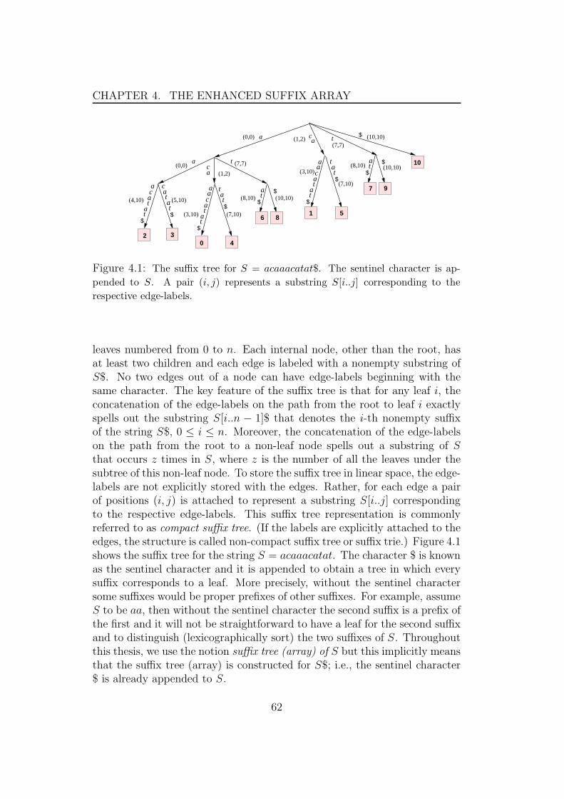
CHAPTER 4. THE ENHANCED SUFFIX ARRAY
2
aca
at
t$
ca
at
t$
at
$
$aaca
at
t$
at
t$
ac a
t
t$
aaca
at
t$
at
$
$
ca t
(10,10)(8,10)
(7,10)(3,10)
(5,10)(4,10)
(7,7)ta(0,0)
(1,2)
(0,0) a $
(7,7)(10,10)
(3,10)
(7,10)
(8,10) (10,10)
(1,2)
3
6 8
0 4
1 5
7 9
10
Figure 4.1: The suffix tree for S = acaaacatat$. The sentinel character is ap-
pended to S. A pair (i, j) represents a substring S[i..j] corresponding to the
respective edge-labels.
leaves numbered from 0 to n. Each internal node, other than the root, hasat least two children and each edge is labeled with a nonempty substring ofS$. No two edges out of a node can have edge-labels beginning with thesame character. The key feature of the suffix tree is that for any leaf i, theconcatenation of the edge-labels on the path from the root to leaf i exactlyspells out the substring S[i..n − 1]$ that denotes the i-th nonempty suffixof the string S$, 0 ≤ i ≤ n. Moreover, the concatenation of the edge-labelson the path from the root to a non-leaf node spells out a substring of Sthat occurs z times in S, where z is the number of all the leaves under thesubtree of this non-leaf node. To store the suffix tree in linear space, the edge-labels are not explicitly stored with the edges. Rather, for each edge a pairof positions (i, j) is attached to represent a substring S[i..j] correspondingto the respective edge-labels. This suffix tree representation is commonlyreferred to as compact suffix tree. (If the labels are explicitly attached to theedges, the structure is called non-compact suffix tree or suffix trie.) Figure 4.1shows the suffix tree for the string S = acaaacatat. The character $ is knownas the sentinel character and it is appended to obtain a tree in which everysuffix corresponds to a leaf. More precisely, without the sentinel charactersome suffixes would be proper prefixes of other suffixes. For example, assumeS to be aa, then without the sentinel character the second suffix is a prefix ofthe first and it will not be straightforward to have a leaf for the second suffixand to distinguish (lexicographically sort) the two suffixes of S. Throughoutthis thesis, we use the notion suffix tree (array) of S but this implicitly meansthat the suffix tree (array) is constructed for S$; i.e., the sentinel character$ is already appended to S.
62
CHAPTER 4. THE ENHANCED SUFFIX ARRAY
The suffix tree is undoubtedly one of the most important data structuresin string processing. It can be constructed and stored in O(n) time and space[101, 137]; see also [62] for more a simplified exposition. Once constructed,it can be used to efficiently solve a myriad of string processing applications[15]. These applications can be broadly classified into the following kinds oftree traversals:
• a bottom-up traversal of the suffix tree
• a top-down traversal of the suffix tree
• a traversal of the suffix tree using suffix links (suffix links will be intro-duced later)
Although suffix trees play a prominent role in algorithmics, they are not aswidespread in actual implementations of software tools as one should expect.There are two major reasons for this:
(i) Although being asymptotically linear, the space consumption of a suffixtree is quite large; even recently improved implementations of lineartime constructions still require 20n bytes (20 bytes per one characterof S) in the worst case; see, e.g., [89].
(ii) In most applications, the suffix tree suffers from a poor locality ofmemory reference, which causes a significant loss of efficiency on cachedprocessor architectures, and renders it difficult to store in secondarymemory.
These problems have been identified in several large scale applications likethe repeat analysis of whole genomes [91] and the comparison of completegenomes [44, 45, 68].
The suffix array is more space efficient data structure than the suffix tree.It was introduced by Manber and Myers [100], and independently by Gonnetet al. [59] under the name PAT array. The suffix array of a string S, whichwe denote by suftab, is an array of integers in the range 0 to n, specifyingthe lexicographic ordering of the n + 1 suffixes of the string S$. That is,S(suftab[0]), S(suftab[1]), . . . , S(suftab[n]) is the sequence of suffixes of S$ inascending lexicographic order; see Figure 4.2. The suffix array requires only4n bytes in its basic form and it can be constructed in O(n) time in theworst case either by first constructing the suffix tree of S [62] or directly bysuffix sorting [75, 83, 85]. However, non-linear time algorithms [26, 93] arestill more efficient in practice.
As already mentioned in [62], if the edges of the suffix tree are lexico-graphically organized (edges out of each internal node are drawn from left to
63
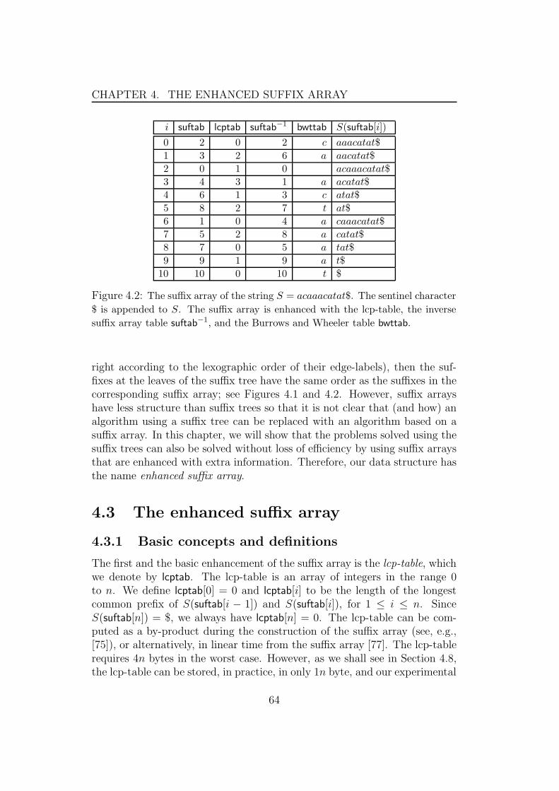
CHAPTER 4. THE ENHANCED SUFFIX ARRAY
i suftab lcptab suftab−1 bwttab S(suftab[i])
0 2 0 2 c aaacatat$
1 3 2 6 a aacatat$
2 0 1 0 acaaacatat$
3 4 3 1 a acatat$
4 6 1 3 c atat$
5 8 2 7 t at$
6 1 0 4 a caaacatat$
7 5 2 8 a catat$
8 7 0 5 a tat$
9 9 1 9 a t$
10 10 0 10 t $
Figure 4.2: The suffix array of the string S = acaaacatat$. The sentinel character
$ is appended to S. The suffix array is enhanced with the lcp-table, the inverse
suffix array table suftab−1, and the Burrows and Wheeler table bwttab.
right according to the lexographic order of their edge-labels), then the suf-fixes at the leaves of the suffix tree have the same order as the suffixes in thecorresponding suffix array; see Figures 4.1 and 4.2. However, suffix arrayshave less structure than suffix trees so that it is not clear that (and how) analgorithm using a suffix tree can be replaced with an algorithm based on asuffix array. In this chapter, we will show that the problems solved using thesuffix trees can also be solved without loss of efficiency by using suffix arraysthat are enhanced with extra information. Therefore, our data structure hasthe name enhanced suffix array.
4.3 The enhanced suffix array
4.3.1 Basic concepts and definitions
The first and the basic enhancement of the suffix array is the lcp-table, whichwe denote by lcptab. The lcp-table is an array of integers in the range 0to n. We define lcptab[0] = 0 and lcptab[i] to be the length of the longestcommon prefix of S(suftab[i − 1]) and S(suftab[i]), for 1 ≤ i ≤ n. SinceS(suftab[n]) = $, we always have lcptab[n] = 0. The lcp-table can be com-puted as a by-product during the construction of the suffix array (see, e.g.,[75]), or alternatively, in linear time from the suffix array [77]. The lcp-tablerequires 4n bytes in the worst case. However, as we shall see in Section 4.8,the lcp-table can be stored, in practice, in only 1n byte, and our experimental
64

CHAPTER 4. THE ENHANCED SUFFIX ARRAY
results reported in Section 4.9 show that this space reduction entails no lossof performance.
We introduce two notions that will be used in some applications of thischapter: the inverse suffix array and the Burrows and Wheeler table. The in-verse suffix array suftab−1 is a table of size n+1 such that suftab−1[suftab[q]] =q for any 0 ≤ q ≤ n. suftab−1 can be computed in linear time from the suf-fix array and needs 4n bytes. The Burrows and Wheeler table, denotedby bwttab, contains the Burrows and Wheeler transformation [35] knownfrom data compression. It is a table of size n + 1 such that for everyi, 0 ≤ i ≤ n, bwttab[i] = S[suftab[i]−1] if suftab[i] 6= 0. bwttab[i] is undefinedif suftab[i] = 0. The table bwttab is stored in 1n bytes and constructed in onescan over the suffix array in O(n) time. Figure 4.2 shows the lcptab, bwttab,and suftab−1 and the corresponding the suffix array.
4.3.2 Applications
In general, the applications of the enhanced suffix array can be categorized inanalogous way to the classification in Section 4.2, presented for the suffix tree.That is, there are three types of algorithms: algorithms based on simulatinga bottom-up traversal on the corresponding suffix tree, algorithms basedon simulating a top-down traversal, and algorithms based on simulating atraversal using suffix links. Furthermore, we present algorithms that exploitsolely the properties of the enhanced suffix array.
Coincidentally, the applications required for genome analysis and com-parison, especially those that are used to compute fragments, fall into allthese classes (recall from Chapter 1 that the fragments are common sub-strings between the sequences in comparison and they should be generatedin the first phase of the anchor based strategy). Therefore, we follow thisscheme for presenting our algorithms. Table 4.1 shows the applications ofgenerating different kinds fragments and shows also which kind of traversalis used for the respective application. Other applications in genome analysis,such as computing exact repeats, tandem repeats, and minimal unique sub-strings will also be discussed. Moreover, we shed light on some applicationsin fields other than genome analysis, such as text compression.
65
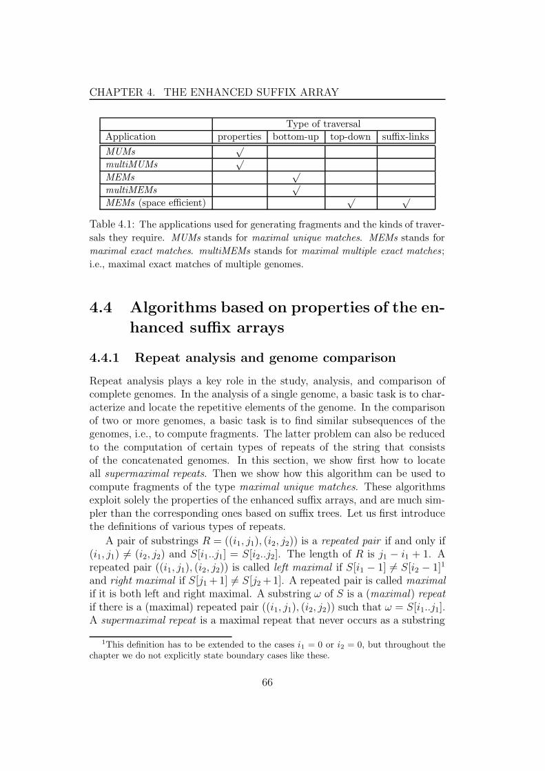
CHAPTER 4. THE ENHANCED SUFFIX ARRAY
Type of traversal
Application properties bottom-up top-down suffix-links
MUMs√
multiMUMs√
MEMs√
multiMEMs√
MEMs (space efficient)√ √
Table 4.1: The applications used for generating fragments and the kinds of traver-
sals they require. MUMs stands for maximal unique matches. MEMs stands for
maximal exact matches. multiMEMs stands for maximal multiple exact matches;
i.e., maximal exact matches of multiple genomes.
4.4 Algorithms based on properties of the en-
hanced suffix arrays
4.4.1 Repeat analysis and genome comparison
Repeat analysis plays a key role in the study, analysis, and comparison ofcomplete genomes. In the analysis of a single genome, a basic task is to char-acterize and locate the repetitive elements of the genome. In the comparisonof two or more genomes, a basic task is to find similar subsequences of thegenomes, i.e., to compute fragments. The latter problem can also be reducedto the computation of certain types of repeats of the string that consistsof the concatenated genomes. In this section, we show first how to locateall supermaximal repeats. Then we show how this algorithm can be used tocompute fragments of the type maximal unique matches. These algorithmsexploit solely the properties of the enhanced suffix arrays, and are much sim-pler than the corresponding ones based on suffix trees. Let us first introducethe definitions of various types of repeats.
A pair of substrings R = ((i1, j1), (i2, j2)) is a repeated pair if and only if(i1, j1) 6= (i2, j2) and S[i1..j1] = S[i2..j2]. The length of R is j1 − i1 + 1. Arepeated pair ((i1, j1), (i2, j2)) is called left maximal if S[i1 − 1] 6= S[i2 − 1]1
and right maximal if S[j1 +1] 6= S[j2 +1]. A repeated pair is called maximalif it is both left and right maximal. A substring ω of S is a (maximal) repeatif there is a (maximal) repeated pair ((i1, j1), (i2, j2)) such that ω = S[i1..j1].A supermaximal repeat is a maximal repeat that never occurs as a substring
1This definition has to be extended to the cases i1 = 0 or i2 = 0, but throughout thechapter we do not explicitly state boundary cases like these.
66

CHAPTER 4. THE ENHANCED SUFFIX ARRAY
g a g c t a g a g c g S:
g a g c t a g a g c g S:
g a g c t a g a g c g
S: g a g c t a g a g c g
S:
0 1 2 3 4 5 6 7 8 9 10
0 1 2 3 4 5 6 7 8 9 10
Figure 4.3: Repeats of the string S = gagctagagcg. Left: three maximal repeated
pairs of minimum length two. The pairs are ((0, 3), (6, 9)), ((1, 2), (5, 6)), and
((5, 6), (7, 8)). Right: one supermaximal repeat of the substrings (0, 3) and (6, 9).
The repeat ag is not supermaximal because it is not maximal and contained in
gagc.
of any other maximal repeat. Figure 4.3 shows maximal repeated pairs andsupermaximal repeats of the string S = gagctagagcg. Now, we introduce thefirst essential concept of this chapter: the lcp-intervals.
4.4.2 The lcp-intervals
Definition 4.4.1 An interval [i..j] of the enhanced suffix array of S, 0 ≤i < j ≤ n, is an lcp-interval of lcp-value ` if
1. lcptab[i] < `,
2. lcptab[k] ≥ ` for all k with i + 1 ≤ k ≤ j,
3. lcptab[k] = ` for at least one k with i + 1 ≤ k ≤ j,
4. lcptab[j + 1] < `.
We will also use the shorthand `-interval (or even `-[i..j]) for an lcp-interval[i..j] of lcp-value `. Every index k, i + 1 ≤ k ≤ j, with lcptab[k] = ` iscalled `-index. The set of all `-indices of an `-interval [i..j] will be denotedby `Indices(i, j). If [i..j] is an `-interval such that ω = S[suftab[i]..suftab[i]+` − 1] is the longest common prefix of the suffixes S(suftab[i]), S(suftab[i +1]), . . . , S(suftab[j]), then [i..j] is called the ω-interval. The size of an interval[i..j] is j − i + 1.
As an example, consider the table in Figure 4.2. The interval [0..5] is a1-interval because lcptab[0] = 0 < 1, lcptab[5 + 1] = 0 < 1, lcptab[k] ≥ 1 forall k with 1 ≤ k ≤ 5, and lcptab[2] = 1. Furthermore, 1-[0..5] is the a-interval(all the suffixes share the prefix ω = a) and `Indices(0, 5) = {2, 4}. We shallsee later that lcp-intervals correspond to internal nodes of the suffix tree.
67
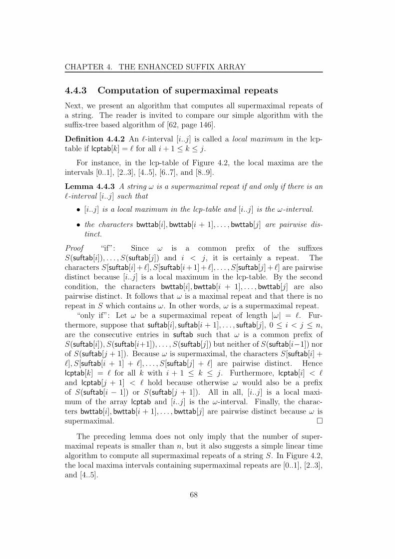
CHAPTER 4. THE ENHANCED SUFFIX ARRAY
4.4.3 Computation of supermaximal repeats
Next, we present an algorithm that computes all supermaximal repeats ofa string. The reader is invited to compare our simple algorithm with thesuffix-tree based algorithm of [62, page 146].
Definition 4.4.2 An `-interval [i..j] is called a local maximum in the lcp-table if lcptab[k] = ` for all i + 1 ≤ k ≤ j.
For instance, in the lcp-table of Figure 4.2, the local maxima are theintervals [0..1], [2..3], [4..5], [6..7], and [8..9].
Lemma 4.4.3 A string ω is a supermaximal repeat if and only if there is an`-interval [i..j] such that
• [i..j] is a local maximum in the lcp-table and [i..j] is the ω-interval.
• the characters bwttab[i], bwttab[i + 1], . . . , bwttab[j] are pairwise dis-tinct.
Proof “if”: Since ω is a common prefix of the suffixesS(suftab[i]), . . . , S(suftab[j]) and i < j, it is certainly a repeat. Thecharacters S[suftab[i]+ `], S[suftab[i+1]+ `], . . . , S[suftab[j]+ `] are pairwisedistinct because [i..j] is a local maximum in the lcp-table. By the secondcondition, the characters bwttab[i], bwttab[i + 1], . . . , bwttab[j] are alsopairwise distinct. It follows that ω is a maximal repeat and that there is norepeat in S which contains ω. In other words, ω is a supermaximal repeat.
“only if”: Let ω be a supermaximal repeat of length |ω| = `. Fur-thermore, suppose that suftab[i], suftab[i + 1], . . . , suftab[j], 0 ≤ i < j ≤ n,are the consecutive entries in suftab such that ω is a common prefix ofS(suftab[i]), S(suftab[i+1]), . . . , S(suftab[j]) but neither of S(suftab[i−1]) norof S(suftab[j + 1]). Because ω is supermaximal, the characters S[suftab[i] +`], S[suftab[i + 1] + `], . . . , S[suftab[j] + `] are pairwise distinct. Hencelcptab[k] = ` for all k with i + 1 ≤ k ≤ j. Furthermore, lcptab[i] < `and lcptab[j + 1] < ` hold because otherwise ω would also be a prefixof S(suftab[i − 1]) or S(suftab[j + 1]). All in all, [i..j] is a local maxi-mum of the array lcptab and [i..j] is the ω-interval. Finally, the charac-ters bwttab[i], bwttab[i + 1], . . . , bwttab[j] are pairwise distinct because ω issupermaximal. �
The preceding lemma does not only imply that the number of super-maximal repeats is smaller than n, but it also suggests a simple linear timealgorithm to compute all supermaximal repeats of a string S. In Figure 4.2,the local maxima intervals containing supermaximal repeats are [0..1], [2..3],and [4..5].
68
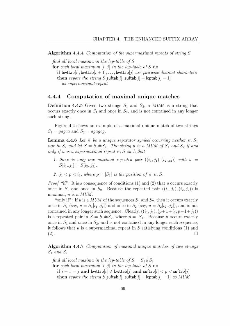
CHAPTER 4. THE ENHANCED SUFFIX ARRAY
Algorithm 4.4.4 Computation of the supermaximal repeats of string S
find all local maxima in the lcp-table of Sfor each local maximum [i..j] in the lcp-table of S do
if bwttab[i], bwttab[i + 1], . . . , bwttab[j] are pairwise distinct charactersthen report the string S[suftab[i]..suftab[i] + lcptab[i] − 1]
as supermaximal repeat
4.4.4 Computation of maximal unique matches
Definition 4.4.5 Given two strings S1 and S2, a MUM is a string thatoccurs exactly once in S1 and once in S2, and is not contained in any longersuch string.
Figure 4.4 shows an example of a maximal unique match of two stringsS1 = gagca and S2 = agagcg.
Lemma 4.4.6 Let # be a unique separator symbol occurring neither in S1
nor in S2 and let S = S1#S2. The string u is a MUM of S1 and S2 if andonly if u is a supermaximal repeat in S such that
1. there is only one maximal repeated pair ((i1, j1), (i2, j2)) with u =S[i1..j1] = S[i2..j2],
2. j1 < p < i2, where p = |S1| is the position of # in S.
Proof “if”: It is a consequence of conditions (1) and (2) that u occurs exactlyonce in S1 and once in S2. Because the repeated pair ((i1, j1), (i2, j2)) ismaximal, u is a MUM .
“only if”: If u is a MUM of the sequences S1 and S2, then it occurs exactlyonce in S1 (say, u = S1[i1..j1]) and once in S2 (say, u = S2[i2..j2]), and is notcontained in any longer such sequence. Clearly, ((i1, j1), (p+1+i2, p+1+j2))is a repeated pair in S = S1#S2, where p = |S1|. Because u occurs exactlyonce in S1 and once in S2, and is not contained in any longer such sequence,it follows that u is a supermaximal repeat in S satisfying conditions (1) and(2). �
Algorithm 4.4.7 Computation of maximal unique matches of two stringsS1 and S2
find all local maxima in the lcp-table of S = S1#S2
for each local maximum [i..j] in the lcp-table of S doif i + 1 = j and bwttab[i] 6= bwttab[j] and suftab[i] < p < suftab[j]then report the string S[suftab[i]..suftab[i] + lcptab[i] − 1] as MUM
69

CHAPTER 4. THE ENHANCED SUFFIX ARRAY
S1
S1
S2
a g a g c g S2
g a g c a
# g a g c a # a g a g c g
Figure 4.4: Maximal unique matches of the strings S1 = gagca and S2 = agagcg.
The maximal unique match that is composed of the substrings gagc (left) is a
supermaximal repeat in S1#S2 (right).
The algorithms that compute supermaximal repeats and MUMs requiretables suftab, lcptab, and bwttab, but do not access the input sequence. Moreprecisely, instead of the input string, we use the table bwttab without increas-ing the total space requirement. This is because the tables suftab, lcptab, andbwttab can be accessed in sequential order, thus leading to an improved cachecoherence and in turn considerably reduced running time; see experimentalresults in Section 4.9.
It is interesting to mention that EMAGEN [46], a recent software tool forcomparing genomes, applied our algorithm for generating MUMs for morethan two genomic sequences. MUMs of more than two genomes are calledmaximal multiple unique matches. Roughly speaking, a multiMUM is amatch that occurs exactly once in each of the given sequences and cannot beextended to the left (left maximal) and to the right (right maximal) simul-taneously. multiMUMs can be formally defined as follows.
Definition 4.4.8 Given k strings S1, S2, . . . , Sk, a multiMUM is a substringSi[li..hi] that occurs exactly once in each of Si, 1 ≤ i ≤ k and there is at leasttwo characters such that Si[li−1] 6= Sj[lj −1] (left maximal) and at least twocharacters such that Si[hi + 1] 6= Sj[hj + 1] (right maximal), 1 ≤ i 6= j ≤ k.
For computing the multiMUMs, the enhanced suffix array is constructedfor S1#S2#..#Sk. The local maximum lcp-intervals are the intervals of sizeexactly k; note that these intervals can enclose other lcp-intervals. A localmaximum lcp-interval [i..i + k − 1] of lcp value `, contains a multiMUM oflength ` if (1) there are no two indices i ≤ i1, i2 ≤ i+k−1 such that suftab[i1]and suftab[i2] are in the same genomic sequence, and (2) the set of charactersbwttab[i], . . . , bwttab[i + k − 1] is composed of at least two characters.
4.5 Bottom-up traversals
In this section, we show how to simulate the bottom-up traversal of the suf-fix tree using the enhanced suffix array. As we mentioned before, the com-
70
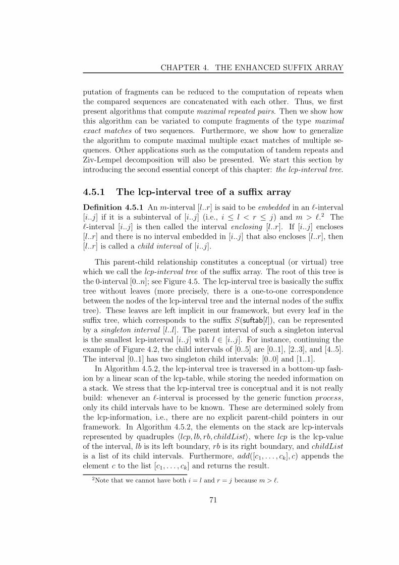
CHAPTER 4. THE ENHANCED SUFFIX ARRAY
putation of fragments can be reduced to the computation of repeats whenthe compared sequences are concatenated with each other. Thus, we firstpresent algorithms that compute maximal repeated pairs. Then we show howthis algorithm can be variated to compute fragments of the type maximalexact matches of two sequences. Furthermore, we show how to generalizethe algorithm to compute maximal multiple exact matches of multiple se-quences. Other applications such as the computation of tandem repeats andZiv-Lempel decomposition will also be presented. We start this section byintroducing the second essential concept of this chapter: the lcp-interval tree.
4.5.1 The lcp-interval tree of a suffix array
Definition 4.5.1 An m-interval [l..r] is said to be embedded in an `-interval[i..j] if it is a subinterval of [i..j] (i.e., i ≤ l < r ≤ j) and m > `.2 The`-interval [i..j] is then called the interval enclosing [l..r]. If [i..j] encloses[l..r] and there is no interval embedded in [i..j] that also encloses [l..r], then[l..r] is called a child interval of [i..j].
This parent-child relationship constitutes a conceptual (or virtual) treewhich we call the lcp-interval tree of the suffix array. The root of this tree isthe 0-interval [0..n]; see Figure 4.5. The lcp-interval tree is basically the suffixtree without leaves (more precisely, there is a one-to-one correspondencebetween the nodes of the lcp-interval tree and the internal nodes of the suffixtree). These leaves are left implicit in our framework, but every leaf in thesuffix tree, which corresponds to the suffix S(suftab[l]), can be representedby a singleton interval [l..l]. The parent interval of such a singleton intervalis the smallest lcp-interval [i..j] with l ∈ [i..j]. For instance, continuing theexample of Figure 4.2, the child intervals of [0..5] are [0..1], [2..3], and [4..5].The interval [0..1] has two singleton child intervals: [0..0] and [1..1].
In Algorithm 4.5.2, the lcp-interval tree is traversed in a bottom-up fash-ion by a linear scan of the lcp-table, while storing the needed information ona stack. We stress that the lcp-interval tree is conceptual and it is not reallybuild: whenever an `-interval is processed by the generic function process,only its child intervals have to be known. These are determined solely fromthe lcp-information, i.e., there are no explicit parent-child pointers in ourframework. In Algorithm 4.5.2, the elements on the stack are lcp-intervalsrepresented by quadruples 〈lcp, lb, rb, childList〉, where lcp is the lcp-valueof the interval, lb is its left boundary, rb is its right boundary, and childListis a list of its child intervals. Furthermore, add([c1, . . . , ck], c) appends theelement c to the list [c1, . . . , ck] and returns the result.
2Note that we cannot have both i = l and r = j because m > `.
71

CHAPTER 4. THE ENHANCED SUFFIX ARRAY
0-[0..10]
q)
q)
2-[0..1] 2-[4..5]?
3-[2..3]
1-[0..5] 1-[8..9]?
2-[6..7]
Figure 4.5: The lcp-interval tree of the string S = acaaacatat. The enhanced
suffix array of this string is the one of Figure 4.2.
Algorithm 4.5.2 Traverse and process the lcp-interval tree
lastInterval := ⊥push(〈0, 0,⊥, [ ]〉)for i := 1 to n do
lb := i − 1while lcptab[i] < top.lcp
top.rb := i − 1lastInterval := popprocess(lastInterval)lb := lastInterval.lbif lcptab[i] ≤ top.lcp then
top.childList := add(top.childList, lastInterval)lastInterval := ⊥
if lcptab[i] > top.lcp thenif lastInterval 6= ⊥ then
push(〈lcptab[i], lb,⊥, [lastInterval]〉)lastInterval := ⊥
else push(〈lcptab[i], lb,⊥, [ ]〉)In the remaining part of this section, several problems will be solved
merely by specifying the function process called in line 8 of Algorithm 4.5.2.It is worth mentioning that the lcp-interval tree takes the approach of Kasaiet al. [77] one step further. They showed how to simulate the bottom-uptraversal of the suffix tree over the suffix array using the lcptab, but, unlikeour algorithm, they did not take the child intervals into account. As a con-sequence, their approach has two limitations: First, it is not straightforwardto systematically replace an algorithm based on the bottom-up traversal ofa suffix tree with an equivalent one on suffix array. Second, it is not possibleto extend their approach to other kinds of suffix tree traversal.
72

CHAPTER 4. THE ENHANCED SUFFIX ARRAY
4.5.2 Computation of maximal repeated pairs
Now, we show how to specify the function process for computing maximalrepeated pairs. We start with introducing some notations: Let ⊥ stand forthe undefined character. We assume that it is different from all charactersin Σ. Let [i..j] be an `-interval and u = S[suftab[i]..suftab[i] + ` − 1]. DefineP[i..j] to be the set of positions p such that u is a prefix of Sp, i.e., P[i..j] ={suftab[r] | i ≤ r ≤ j}. We divide P[i..j] into disjoint and possibly empty setsaccording to the characters to the left of each position: For any a ∈ Σ∪ {⊥}define
P[i..j](a) =
{
{0 | 0 ∈ P[i..j]} if a = ⊥{p | p ∈ P[i..j], p > 0, and S[p − 1] = a} otherwise
The algorithm computes position sets in a bottom-up strategy. In termsof an lcp-interval tree, this means that the lcp-interval [i..j] is processed onlyafter all child intervals of [i..j] have been processed.
Suppose [i..j] is a singleton interval, i.e., i = j. Let p = suftab[i]. ThenP[i..j] = {p} and
P[i..j](a) =
{
{p} if p > 0 and S[p − 1] = a or p = 0 and a = ⊥∅ otherwise
In the implementation, we do not access S to determine the character S[p−1].Instead, we use the bwttab table to improve the cash performance of thealgorithm by avoiding random access to the string.
Now suppose that [i..j] is not singleton interval, i.e., i < j. For each a ∈Σ∪{⊥}, P[i..j](a) is computed step by step while processing the child intervalsof [i..j]. Suppose that we have already processed the first q child intervalsof [i..j]. Let P1..q
[i..j](a) denote the subset of P[i..j](a) obtained after processing
the q-th child interval of [i..j]. Let [i′..j ′] be the (q + 1)-th child interval of[i..j]. Due to the bottom-up strategy, [i′..j ′] has already been processed andhence its position sets P[i′..j′](b) are available for any b ∈ Σ ∪ {⊥}.
The interval [i′..j ′] is processed in the following way. Maximal repeatedpairs are output by combining the position set P1..q
[i..j](a), a ∈ Σ ∪ {⊥}, with
position sets P[i′..j′](b), b ∈ Σ∪{⊥}. In particular, ((p, p+`−1), (p′, p′+`−1)),
p < p′, are output for all p ∈ P1..q
[i..j](a) and p′ ∈ P[i′..j′](b), a, b ∈ Σ ∪ {⊥}and a 6= b. It is clear that u occurs at positions p and p′. Hence ((p, p + ` −1), (p′, p′ + ` − 1)) is a repeated pair. By construction, only those positionsp and p′ are combined for which the characters immediately to the left, i.e.,at positions p − 1 and p′ − 1 (if they exist), are different. This guaranteesleft-maximality of the output repeated pairs. The position sets P1..q
[i..j](a) were
73

CHAPTER 4. THE ENHANCED SUFFIX ARRAY
inherited from child intervals of [i..j] that are different from [i′..j ′]. Hencethe characters immediately to the right of u at positions p + ` and p′ + ` (ifthey exist) are different. As a consequence, the output repeated pairs aremaximal.
Once the maximal repeated pairs for the current child interval [i′..j ′] havebeen output, the union P1..q+1
[i..j] (e) := P1..q
[i..j](e) ∪ P[i′..j′](e) is computed for all
e ∈ Σ ∪ {⊥}. That is, the position sets are inherited from [i′..j ′] to [i..j].
In Algorithm 4.5.2, if the function process is applied to an lcp-interval,then all its child intervals are available. Hence, the maximal repeated pairalgorithm can be implemented by a bottom-up traversal of the lcp-intervaltree. To this end, the function process in Algorithm 4.5.2 outputs maximalrepeated pairs and further maintains position sets on the stack (which areadded as a fifth component to the quadruples).
There are two operations performed when processing an lcp-interval [i..j]:First, output of maximal repeated pairs by combining position sets. Second,union of position sets. Each combination of position sets means to computetheir Cartesian product. This delivers a list of position pairs, i.e., maximalrepeated pairs. Each repeated pair is computed in constant time from theposition lists. Altogether, the combinations can be computed in O(z) time,where z is the number of repeats. The union operation for the position setscan be implemented in constant time, if we use linked lists. For each lcp-interval, we have O(|Σ|) union operations. Since O(n) lcp-intervals have to beprocessed, the union and add operations require O(|Σ|n) time. Altogether,the algorithm runs in O(|Σ|n + z) time.
This algorithm requires linear space. A position set P[i..j](a) is the unionof position sets of the child intervals of [i..j]. Hence it is not required to copyposition sets, rather they are linked together. Moreover, we only have to storethe position sets for those lcp-intervals which are on the stack used for thebottom-up traversal of the lcp-interval tree. So it is natural to store, on thestack, references to the position sets together with other information aboutthe lcp-interval. Thus the space required for the position sets is determinedby the maximal size of the stack. Since this is O(n), the space requirementis O(|Σ|n). In practice, however, the stack size is much smaller. Altogetherthe algorithm is optimal, since its space and time requirement is linear in thesize of the input plus the output.
It is worth mentioning that the above-mentioned algorithm is the en-hanced suffix array version of the algorithm of Gusfield based on the suffixtree [62, page 147]. Gusfield’s Algorithm computes maximal repeated pairsof a sequence S of length n in O(|Σ|n + z) time, where z is the number ofmaximal repeated pairs. To the best of our knowledge, Gusfield’s algorithm
74
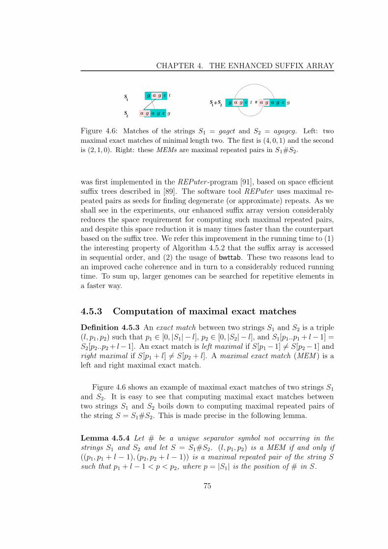
CHAPTER 4. THE ENHANCED SUFFIX ARRAY
1S S
2# g a g c t # a g a g c g
a g a g c g
S
S
1
2
g a g c t
Figure 4.6: Matches of the strings S1 = gagct and S2 = agagcg. Left: two
maximal exact matches of minimal length two. The first is (4, 0, 1) and the second
is (2, 1, 0). Right: these MEMs are maximal repeated pairs in S1#S2.
was first implemented in the REPuter -program [91], based on space efficientsuffix trees described in [89]. The software tool REPuter uses maximal re-peated pairs as seeds for finding degenerate (or approximate) repeats. As weshall see in the experiments, our enhanced suffix array version considerablyreduces the space requirement for computing such maximal repeated pairs,and despite this space reduction it is many times faster than the counterpartbased on the suffix tree. We refer this improvement in the running time to (1)the interesting property of Algorithm 4.5.2 that the suffix array is accessedin sequential order, and (2) the usage of bwttab. These two reasons lead toan improved cache coherence and in turn to a considerably reduced runningtime. To sum up, larger genomes can be searched for repetitive elements ina faster way.
4.5.3 Computation of maximal exact matches
Definition 4.5.3 An exact match between two strings S1 and S2 is a triple(l, p1, p2) such that p1 ∈ [0, |S1| − l], p2 ∈ [0, |S2| − l], and S1[p1..p1 + l− 1] =S2[p2..p2 + l− 1]. An exact match is left maximal if S[p1 − 1] 6= S[p2 − 1] andright maximal if S[p1 + l] 6= S[p2 + l]. A maximal exact match (MEM ) is aleft and right maximal exact match.
Figure 4.6 shows an example of maximal exact matches of two strings S1
and S2. It is easy to see that computing maximal exact matches betweentwo strings S1 and S2 boils down to computing maximal repeated pairs ofthe string S = S1#S2. This is made precise in the following lemma.
Lemma 4.5.4 Let # be a unique separator symbol not occurring in thestrings S1 and S2 and let S = S1#S2. (l, p1, p2) is a MEM if and only if((p1, p1 + l − 1), (p2, p2 + l − 1)) is a maximal repeated pair of the string Ssuch that p1 + l − 1 < p < p2, where p = |S1| is the position of # in S.
75
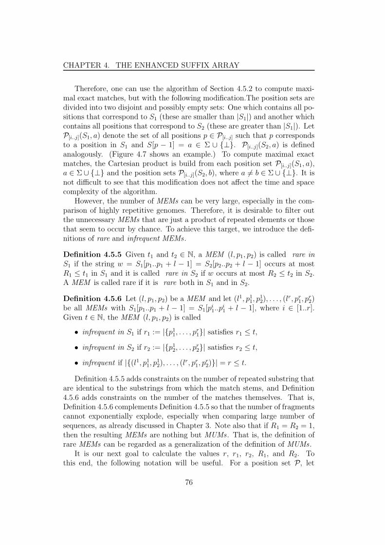
CHAPTER 4. THE ENHANCED SUFFIX ARRAY
Therefore, one can use the algorithm of Section 4.5.2 to compute maxi-mal exact matches, but with the following modification.The position sets aredivided into two disjoint and possibly empty sets: One which contains all po-sitions that correspond to S1 (these are smaller than |S1|) and another whichcontains all positions that correspond to S2 (these are greater than |S1|). LetP[i..j](S1, a) denote the set of all positions p ∈ P[i..j] such that p correspondsto a position in S1 and S[p − 1] = a ∈ Σ ∪ {⊥}. P[i..j](S2, a) is definedanalogously. (Figure 4.7 shows an example.) To compute maximal exactmatches, the Cartesian product is build from each position set P[i..j](S1, a),a ∈ Σ ∪ {⊥} and the position sets P[i..j](S2, b), where a 6= b ∈ Σ ∪ {⊥}. It isnot difficult to see that this modification does not affect the time and spacecomplexity of the algorithm.
However, the number of MEMs can be very large, especially in the com-parison of highly repetitive genomes. Therefore, it is desirable to filter outthe unnecessary MEMs that are just a product of repeated elements or thosethat seem to occur by chance. To achieve this target, we introduce the defi-nitions of rare and infrequent MEMs.
Definition 4.5.5 Given t1 and t2 ∈ N, a MEM (l, p1, p2) is called rare inS1 if the string w = S1[p1..p1 + l − 1] = S2[p2..p2 + l − 1] occurs at mostR1 ≤ t1 in S1 and it is called rare in S2 if w occurs at most R2 ≤ t2 in S2.A MEM is called rare if it is rare both in S1 and in S2.
Definition 4.5.6 Let (l, p1, p2) be a MEM and let (l1, p11, p
12), . . . , (l
r, pr1, p
r2)
be all MEMs with S1[p1..p1 + l − 1] = S1[pi1..p
i1 + l − 1], where i ∈ [1..r].
Given t ∈ N, the MEM (l, p1, p2) is called
• infrequent in S1 if r1 := |{p11, . . . , p
r1}| satisfies r1 ≤ t,
• infrequent in S2 if r2 := |{p12, . . . , p
r2}| satisfies r2 ≤ t,
• infrequent if |{(l1, p11, p
12), . . . , (l
r, pr1, p
r2)}| = r ≤ t.
Definition 4.5.5 adds constraints on the number of repeated substring thatare identical to the substrings from which the match stems, and Definition4.5.6 adds constraints on the number of the matches themselves. That is,Definition 4.5.6 complements Definition 4.5.5 so that the number of fragmentscannot exponentially explode, especially when comparing large number ofsequences, as already discussed in Chapter 3. Note also that if R1 = R2 = 1,then the resulting MEMs are nothing but MUMs. That is, the definition ofrare MEMs can be regarded as a generalization of the definition of MUMs.
It is our next goal to calculate the values r, r1, r2, R1, and R2. Tothis end, the following notation will be useful. For a position set P, let
76
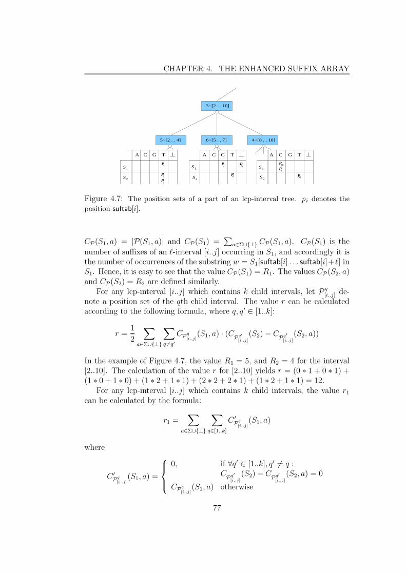
CHAPTER 4. THE ENHANCED SUFFIX ARRAY
S2
S1
S2
S1
S2
S1
p2
p3
p8
p6
A C G T A C G T CA G T
p9
p10
5−[2 . . 4] 6−[5 . . 7] 4−[8 . . 10]
p4
p7
p5
3−[2 . . 10]
Figure 4.7: The position sets of a part of an lcp-interval tree. pi denotes the
position suftab[i].
CP(S1, a) = |P(S1, a)| and CP(S1) =∑
a∈Σ∪{⊥} CP(S1, a). CP(S1) is the
number of suffixes of an `-interval [i..j] occurring in S1, and accordingly it isthe number of occurrences of the substring w = S1[suftab[i] . . . suftab[i]+`] inS1. Hence, it is easy to see that the value CP(S1) = R1. The values CP(S2, a)and CP(S2) = R2 are defined similarly.
For any lcp-interval [i..j] which contains k child intervals, let P q
[i..j] de-note a position set of the qth child interval. The value r can be calculatedaccording to the following formula, where q, q′ ∈ [1..k]:
r =1
2
∑
a∈Σ∪{⊥}
∑
q 6=q′
CPq
[i..j](S1, a) · (C
Pq′
[i..j]
(S2) − CPq′
[i..j]
(S2, a))
In the example of Figure 4.7, the value R1 = 5, and R2 = 4 for the interval[2..10]. The calculation of the value r for [2..10] yields r = (0 ∗ 1 + 0 ∗ 1) +(1 ∗ 0 + 1 ∗ 0) + (1 ∗ 2 + 1 ∗ 1) + (2 ∗ 2 + 2 ∗ 1) + (1 ∗ 2 + 1 ∗ 1) = 12.
For any lcp-interval [i..j] which contains k child intervals, the value r1
can be calculated by the formula:
r1 =∑
a∈Σ∪{⊥}
∑
q∈[1..k]
C ′Pq
[i..j](S1, a)
where
C ′Pq
[i..j](S1, a) =
0, if ∀q′ ∈ [1..k], q′ 6= q :C
Pq′
[i..j]
(S2) − CPq′
[i..j]
(S2, a) = 0
CPq
[i..j](S1, a) otherwise
77
CHAPTER 4. THE ENHANCED SUFFIX ARRAY
In the example of Figure 4.7, we have r1 = 0 + 2 + 1 + 0 + 1 = 4. It isobvious how the algorithm for the computation of MEMs has to be modifiedto compute infrequent MEMs. Clearly, MEMs that occur too many timesseem to have occurred by chance and should be excluded from the set ofpotential anchors. In our opinion, the exact definition of “too many times”depends on the genomes in comparison and should be left to the user ofthe genome comparison tool. In other words, we let the thresholds on thevalues r, r1, r2, R1, and R2 (or a combination of them) as parameters of theprogram.
4.5.4 Computation of maximal multiple exact matches
The notion of maximal multiple exact matches (multiMEMs) is the naturalextension of maximal exact matches to more than two genomes. Roughlyspeaking, a multiMEM is a sequence that occurs in all genomes to be com-pared and cannot simultaneously be extended to the left or to the right inall genomes. The algorithm of Section 4.5.3 can also be modified such thatit computes multiMEMs. More precisely, for the genomes S1, .., Sk, we con-struct the enhanced suffix array of the concatenated genomes S1#1S2#2...#k−1Sk$, where #1, ..., #k−1 are unique separator characters in none ofS1, .., Sk. During the bottom-up traversal, the position sets are constructedw.r.t. every genome. The Cartesian product is then performed over thenon-empty k position sets; i.e., it will be k-dimensional Cartesian prod-uct. It is not difficult to see that the time complexity of the algorithm isO(|S1| + .. + |Sk| + z), where z is the number of multiMEMs, and the spacerequirement is O(|S1| + .. + |Sk|). It is also not difficult to incorporate thenotions of rare and infrequent multiMEMs. These notions, as discussed inChapter 3, are of special importance, because they control the number of thefragments, which grows exponentially with the number of the sequences.
4.5.5 Other applications of the bottom-up traversal
In this subsection, we present two other applications based on bottom-uptraversal of the enhanced suffix array. The first is finding all tandem repeatsof a genomic sequence and the second is computing the Ziv-Lempel decom-position of a string. The former is important for studying genome repetitionsand the later is important for data compression.
78

CHAPTER 4. THE ENHANCED SUFFIX ARRAY
Tandem repeats
As already mentioned in Chapter 2, repeats play an important role in molec-ular biology, and a basic task is to locate and compile repetitions in a genome.If the repeated segments are occurring adjacent to each other, then we speakof tandem repeats. Formally, a substring of S is a tandem repeat if it canbe written as ωω for some nonempty string ω. An occurrence of a tandemrepeat ωω = S[p..p + 2|ω| − 1] is represented by the pair (p, |ω|). Such anoccurrence (p, |ω|) is branching if S[p + |ω|] 6= S[p + 2|ω|]. There is an abun-dance of papers dealing with the efficient computation of tandem repeats;see, e.g., [130] for references. It is known that tandem repeats of a string Scan be computed in O(n) time in the worst case; see [63, 86]. However, thesealgorithms are quite complicated and do not basically depend on suffix trees(suffix arrays). Therefore, we will present algorithms that are simpler andbased only on enhanced suffix arrays. Experimental results show that ouralgorithms are more efficient in practice, albeit with non-optimal worst casetime complexities.
Stoye and Gusfield [130] described how all tandem repeats can be derivedfrom branching tandem repeats by successively shifting a window to the left;see Figure 4.8. For this reason, we restrict ourselves to the computation ofall branching tandem repeats.
The optimized basic algorithm of [130] computes all branching tandemrepeats in O(n log n) time. It is based on a traversal of the suffix tree, inwhich each branching node is annotated by its leaf list, i.e., by the set of leavesin the subtree below it. The leaf list of a branching node corresponds to anlcp-interval in the lcp-interval tree. As a consequence, it is not difficult toimplement the optimized basic algorithm via a traversal of the lcp-intervaltree. For ease of presentation, we start with the basic algorithm of [130],which is based on the following lemma.
Lemma 4.5.7 Let ω = S[p..p + ` − 1], where ` = |ω| > 0, and let [i..j] bethe ω-interval. The following statements are equivalent.
1. (p, `) is an occurrence of a branching tandem repeat.
2. i ≤ suftab−1[p] ≤ j and i ≤ suftab−1[p+ `] ≤ j and S[p+ `] 6= S[p+2`].
Proof (1) ⇒ (2): If (p, `) is an occurrence of the tandem repeat ω, thenω = S[p..p + ` − 1] = S[p + `..p + 2` − 1]. Since ω is the longest commonprefix of S(suftab[i]), . . . , S(suftab[j]), it follows that i ≤ suftab−1[p] ≤ j andi ≤ suftab−1[p + `] ≤ j. Furthermore, S[p + `] 6= S[p + 2`] because (p, `) isbranching.
79
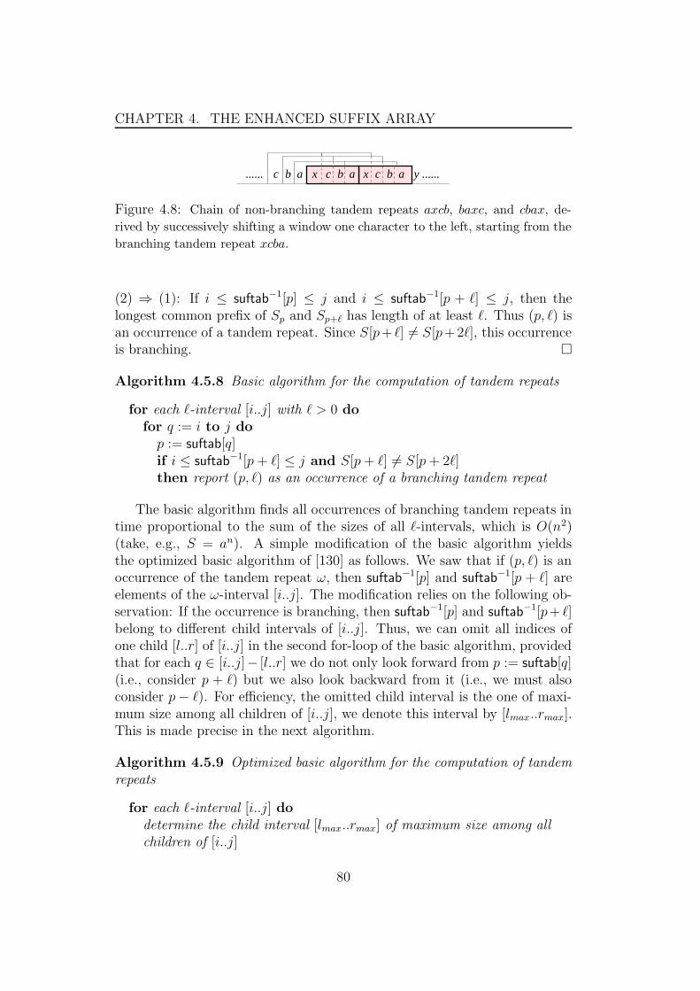
CHAPTER 4. THE ENHANCED SUFFIX ARRAY
x...... y ......xac b ac bac b
Figure 4.8: Chain of non-branching tandem repeats axcb, baxc, and cbax, de-
rived by successively shifting a window one character to the left, starting from the
branching tandem repeat xcba.
(2) ⇒ (1): If i ≤ suftab−1[p] ≤ j and i ≤ suftab−1[p + `] ≤ j, then thelongest common prefix of Sp and Sp+` has length of at least `. Thus (p, `) isan occurrence of a tandem repeat. Since S[p+ `] 6= S[p+2`], this occurrenceis branching. �
Algorithm 4.5.8 Basic algorithm for the computation of tandem repeats
for each `-interval [i..j] with ` > 0 dofor q := i to j do
p := suftab[q]if i ≤ suftab−1[p + `] ≤ j and S[p + `] 6= S[p + 2`]then report (p, `) as an occurrence of a branching tandem repeat
The basic algorithm finds all occurrences of branching tandem repeats intime proportional to the sum of the sizes of all `-intervals, which is O(n2)(take, e.g., S = an). A simple modification of the basic algorithm yieldsthe optimized basic algorithm of [130] as follows. We saw that if (p, `) is anoccurrence of the tandem repeat ω, then suftab−1[p] and suftab−1[p + `] areelements of the ω-interval [i..j]. The modification relies on the following ob-servation: If the occurrence is branching, then suftab−1[p] and suftab−1[p+ `]belong to different child intervals of [i..j]. Thus, we can omit all indices ofone child [l..r] of [i..j] in the second for-loop of the basic algorithm, providedthat for each q ∈ [i..j]− [l..r] we do not only look forward from p := suftab[q](i.e., consider p + `) but we also look backward from it (i.e., we must alsoconsider p − `). For efficiency, the omitted child interval is the one of maxi-mum size among all children of [i..j], we denote this interval by [lmax..rmax].This is made precise in the next algorithm.
Algorithm 4.5.9 Optimized basic algorithm for the computation of tandemrepeats
for each `-interval [i..j] dodetermine the child interval [lmax..rmax] of maximum size among allchildren of [i..j]
80
CHAPTER 4. THE ENHANCED SUFFIX ARRAY
for q ∈ [i..j] − [lmax..rmax] dop := suftab[q]if i ≤ suftab−1[p + `] ≤ j and S[p + `] 6= S[p + 2`]then report (p, `) as an occurrence of a branching tandem repeatif i ≤ suftab−1[p − `] ≤ j and S[p − `] 6= S[p + `]then report (p − `, `) as an occurrence of a branching tandem repeat
Algorithm 4.5.9 can be implemented by a bottom-up traversal of thelcp-interval tree. Then, for each `-interval, a child interval of maximumsize can be determined in constant time. Since the largest child intervalis always excluded in the second for-loop of Algorithm 4.5.9, the algorithmruns in O(n logn) time; see [130]. Algorithm 4.5.9 requires the tables lcptab,suftab, and suftab−1 plus some space for the stack used during the bottom-uptraversal of the lcp-interval tree.
We further improve Algorithm 4.5.9 by getting rid of the character-checksand reducing the number of forward- and backward checks. That is, weexploit the fact that for an occurrence (|ω|, p) of a branching tandem repeatωω, we have S[p] = S[p + |ω|]. As a consequence, if p + |ω| = suftab[q] forsome q in the ω-interval [i..j], p must occur in the child interval [la..ra] storingthe suffixes of S that have ωa as a prefix, where a = S[suftab[i]] = S[p]. Thisis formally stated in the following lemma.
Lemma 4.5.10 The following statements are equivalent:
(1) (|ω|, p) is an occurrence of a branching tandem repeat ωω.
(2) p+ |ω| = suftab[q] for some q in the ω-interval [i..j], and p = suftab[qa]for some qa in the child interval [ia..ja] representing the suffixes of Sthat have ωa as a prefix, where a = S[p].
This lemma suggests the following algorithm:
Algorithm 4.5.11 For each `-interval [i..j], let a = S[suftab[i]] and deter-mine the child interval [ia..ja] of [i..j] such that a = S[suftab[ia]+ `]. Proceedaccording to the following cases:
(1) If ja − ia + 1 ≤ i − j + 1 − (ja − ia + 1), then for each q, ia ≤ q ≤ ja,let p = suftab[q]. If p + ` = suftab[r] for some r, i ≤ r ≤ ia − 1 orja + 1 ≤ r ≤ j, then output (`, p).
(2) If ja − ia + 1 > i− j + 1− (ja − ia + 1), then for each q, i ≤ q ≤ ia − 1or ja + 1 ≤ q ≤ j, let p = suftab[q]. If p − ` = suftab[r] for some r,ia ≤ r ≤ ja, then output (`, p).
81
CHAPTER 4. THE ENHANCED SUFFIX ARRAY
One easily verifies for each interval [l..r] that l−r+1−(rmax− lmax +1) ≥min{ra − l + 1, l − r + 1− (ra − la + 1)}. Hence Algorithm 4.5.11 checks notmore suffixes than Algorithm 4.5.9. Thus the number of suffixes checkedis O(n log n). For each suffix either a forward-check or backward-check isnecessary. This takes constant time. The lcp-interval tree is processed inO(n) time. Additionally, for each interval the algorithm determines the childinterval [la..ra]. This takes constant extra time. Hence the running time ofAlgorithm 4.5.11 is O(n log n).
Ziv-Lempel decomposition
As a second application of the bottom-up traversal of the lcp-interval tree, wewill describe how to compute the Ziv-Lempel decomposition [142] of a string.The Ziv-Lempel decomposition plays an important role in data compression,and recently it was used in linear time algorithms for the detection of alltandem repeats of a string [63, 86].
For each position i of S, let li denote the length of the longest prefix ofS[i..n] that also occurs as a substring of S starting at some position j < i.Let si denote the starting position of the leftmost occurrence of this substringin S if li > 0, and si = 0, otherwise; see the upper table of Figure 4.9.
The Ziv-Lempel decomposition of S is the list of indices i1, i2, . . . , ik,defined inductively by i1 = 0 and iB+1 = iB + max{1, liB} for B ≥ 1 andiB ≤ n. The substring S[iB..iB+1 − 1], 1 ≤ B ≤ k, obtained in this way iscalled the B-th block of the Ziv-Lempel decomposition of S; see the lowertable of Figure 4.9.
The Ziv-Lempel decomposition of a string S can also be computed off-line in linear time by a bottom-up traversal of the lcp-interval tree; seeAlgorithm 4.5.2. To this end, we add another value min of type integer tothe quadruples stored on the stack. This value corresponds to a position inS. It is initially set to ⊥ and will be updated by the process function. At anystage, when the function process is applied to an `-interval [i..j], all its childintervals are known and have already been processed (note that [i..j] 6= [0..n]must hold). Let [l1..r1], [l2..r2], . . . , [lk..rk] be the k child intervals of [i..j],stored in its childList. Let min1, . . . , mink be the respective min-value ofthe child intervals, where minj = min{suftab[lj], .., suftab[rj]}. Let M be alist of positions in S such that
M = {min1, ..,mink} ∪ {suftab[q] | q ∈ [i..j] and q 6∈ [lp..rp] for all p ∈ [1..k]}
Note that the q indices correspond to singleton intervals. Compute min :=min M and update it in the quadrable of [i..j]. Assign for all p ∈ M withp 6= min: sp := min and lp := `. Finally, for the root [0..n] of the lcp-intervaltree, we assign for all p ∈ M : sp := 0 and lp := 0.
82
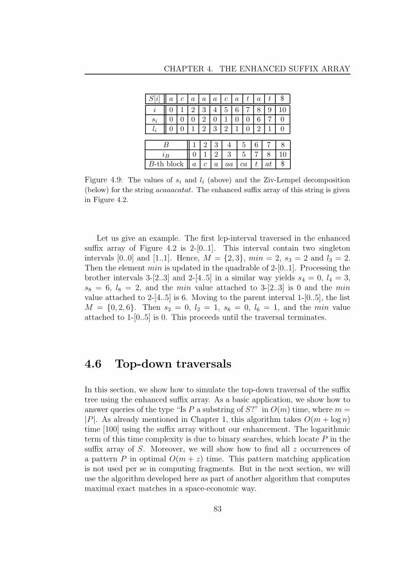
CHAPTER 4. THE ENHANCED SUFFIX ARRAY
S[i] a c a a a c a t a t $
i 0 1 2 3 4 5 6 7 8 9 10
si 0 0 0 2 0 1 0 0 6 7 0
li 0 0 1 2 3 2 1 0 2 1 0
B 1 2 3 4 5 6 7 8
iB 0 1 2 3 5 7 8 10
B-th block a c a aa ca t at $
Figure 4.9: The values of si and li (above) and the Ziv-Lempel decomposition
(below) for the string acaaacatat. The enhanced suffix array of this string is given
in Figure 4.2.
Let us give an example. The first lcp-interval traversed in the enhancedsuffix array of Figure 4.2 is 2-[0..1]. This interval contain two singletonintervals [0..0] and [1..1]. Hence, M = {2, 3}, min = 2, s3 = 2 and l3 = 2.Then the element min is updated in the quadrable of 2-[0..1]. Processing thebrother intervals 3-[2..3] and 2-[4..5] in a similar way yields s4 = 0, l4 = 3,s8 = 6, l8 = 2, and the min value attached to 3-[2..3] is 0 and the minvalue attached to 2-[4..5] is 6. Moving to the parent interval 1-[0..5], the listM = {0, 2, 6}. Then s2 = 0, l2 = 1, s6 = 0, l6 = 1, and the min valueattached to 1-[0..5] is 0. This proceeds until the traversal terminates.
4.6 Top-down traversals
In this section, we show how to simulate the top-down traversal of the suffixtree using the enhanced suffix array. As a basic application, we show how toanswer queries of the type “Is P a substring of S?” in O(m) time, where m =|P |. As already mentioned in Chapter 1, this algorithm takes O(m + log n)time [100] using the suffix array without our enhancement. The logarithmicterm of this time complexity is due to binary searches, which locate P in thesuffix array of S. Moreover, we will show how to find all z occurrences ofa pattern P in optimal O(m + z) time. This pattern matching applicationis not used per se in computing fragments. But in the next section, we willuse the algorithm developed here as part of another algorithm that computesmaximal exact matches in a space-economic way.
83

CHAPTER 4. THE ENHANCED SUFFIX ARRAY
4.6.1 Exact pattern matching
To achieve the O(m+z) time complexity, one must be able to determine, forany `-interval [i..j], all its child intervals in constant time. We achieve thisgoal by enhancing the suffix array with the lcp-table and an additional table:the child-table childtab; see Figure 4.10. The child-table is a table of sizen + 1 indexed from 0 to n and each entry contains three values: up, down,and next`Index. We show later that the three fields can be merged in atable of one column. Each of these three values requires 4 bytes in the worstcase, but in practice it is possible to store the same information in only onebyte; see Section 4.8. Formally, the values of each childtab-entry are definedas follows (we assume that min ∅ = max ∅ = ⊥):
childtab[i].up = min{q ∈ [0..i − 1] | lcptab[q] > lcptab[i] and∀k ∈ [q + 1..i − 1] : lcptab[k] ≥ lcptab[q]}
childtab[i].down = max{q ∈ [i + 1..n] | lcptab[q] > lcptab[i] and∀k ∈ [i + 1..q − 1] : lcptab[k] > lcptab[q]}
childtab[i].next`Index = min{q ∈ [i + 1..n] | lcptab[q] = lcptab[i] and∀k ∈ [i + 1..q − 1] : lcptab[k] > lcptab[i]}
In essence, the child-table stores the parent-child relationship of lcp-intervals. Roughly speaking, for an `-interval [i..j] whose `-indices are i1 <i2 < · · · < ik, the childtab[i].down or childtab[j + 1].up value is used to deter-mine the first `-index i1. The other `-indices i2, . . . ik can be obtained fromchildtab[i1].next`Index, . . . childtab[ik−1].next`Index, respectively. Once allthese `-indices are known, one can determine all the child intervals of [i..j]according to the following lemma.
Lemma 4.6.1 Let [i..j] be an `-interval. If i1 < i2 < · · · < ik are the `-indices in ascending order, then the child intervals of [i..j] are [i..i1 − 1],[i1..i2 − 1], . . . , [ik..j] (note that some of them may be singleton intervals).
Proof Let [l..r] be one of the intervals [i..i1−1], [i1..i2−1], . . . , [ik..j]. If [l..r]is a singleton interval, then it is a child interval of [i..j]. Suppose that [l..r]is an m-interval. Since [l..r] does not contain an `-index, it follows that [l..r]is embedded in [i..j]. Because lcptab[i1] = lcptab[i2] = · · · = lcptab[ik] = `,there is no interval embedded in [i..j] that encloses [l..r]. That is, [l..r] isa child interval of [i..j]. Finally, it is not difficult to see that [i..i1 − 1],[i1..i2 − 1], . . . , [ik..j] are all the child intervals of [i..j], i.e., there cannot beany other child interval. �
As an example, consider the enhanced suffix array in Figure 4.10. The1-[0..5] interval has the 1-indices 2 and 4. The first 1-index 2 is stored in
84
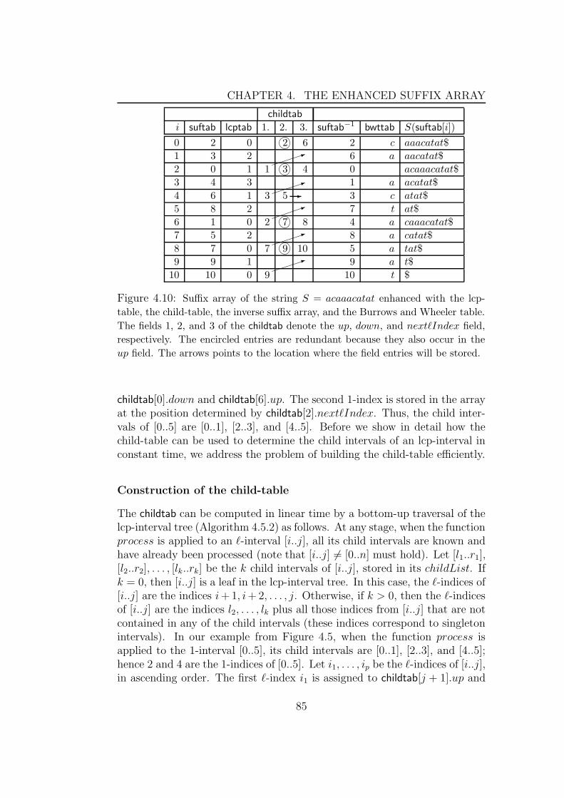
CHAPTER 4. THE ENHANCED SUFFIX ARRAY
-
1
1
1
1
1
childtab
i suftab lcptab 1. 2. 3. suftab−1 bwttab S(suftab[i])
0 2 0 2 6 2 c aaacatat$
1 3 2 6 a aacatat$
2 0 1 1 3 4 0 acaaacatat$
3 4 3 1 a acatat$
4 6 1 3 5 3 c atat$
5 8 2 7 t at$
6 1 0 2 7 8 4 a caaacatat$
7 5 2 8 a catat$
8 7 0 7 9 10 5 a tat$
9 9 1 9 a t$
10 10 0 9 10 t $
Figure 4.10: Suffix array of the string S = acaaacatat enhanced with the lcp-
table, the child-table, the inverse suffix array, and the Burrows and Wheeler table.
The fields 1, 2, and 3 of the childtab denote the up, down, and next`Index field,
respectively. The encircled entries are redundant because they also occur in the
up field. The arrows points to the location where the field entries will be stored.
childtab[0].down and childtab[6].up. The second 1-index is stored in the arrayat the position determined by childtab[2].next`Index. Thus, the child inter-vals of [0..5] are [0..1], [2..3], and [4..5]. Before we show in detail how thechild-table can be used to determine the child intervals of an lcp-interval inconstant time, we address the problem of building the child-table efficiently.
Construction of the child-table
The childtab can be computed in linear time by a bottom-up traversal of thelcp-interval tree (Algorithm 4.5.2) as follows. At any stage, when the functionprocess is applied to an `-interval [i..j], all its child intervals are known andhave already been processed (note that [i..j] 6= [0..n] must hold). Let [l1..r1],[l2..r2], . . . , [lk..rk] be the k child intervals of [i..j], stored in its childList. Ifk = 0, then [i..j] is a leaf in the lcp-interval tree. In this case, the `-indices of[i..j] are the indices i + 1, i + 2, . . . , j. Otherwise, if k > 0, then the `-indicesof [i..j] are the indices l2, . . . , lk plus all those indices from [i..j] that are notcontained in any of the child intervals (these indices correspond to singletonintervals). In our example from Figure 4.5, when the function process isapplied to the 1-interval [0..5], its child intervals are [0..1], [2..3], and [4..5];hence 2 and 4 are the 1-indices of [0..5]. Let i1, . . . , ip be the `-indices of [i..j],in ascending order. The first `-index i1 is assigned to childtab[j + 1].up and
85

CHAPTER 4. THE ENHANCED SUFFIX ARRAY
childtab[i].down. The other `-indices i2, . . . , ip are stored in the next`Indexfield of childtab[i1], childtab[i2], . . . , childtab[ip−1], respectively. Finally, onehas to determine the 0-indices j1, . . . , jq (in ascending order) of the interval[0..n] (which remained on the stack) and store them in the next`Index field ofchildtab[j1], childtab[j2], . . . , childtab[jq−1]. The resulting child-table is shownin Figure 4.10, where the fields 1, 2, and 3 of the childtab denote the up,down, and next`Index field.
Merging the three fields
To reduce the space requirement of the child table, we merge the three fieldsup, down, and next`Index in one array. The basic observation is that thereare O(n) intervals that can determined by a total of O(n) `-indices. Thedetails are as follows. The down field is needed only if it does not containthe same information as the up field. Fortunately, for an `-interval, only onedown field is required because an `-interval [i..j] with k `-indices has at mostk + 1 child intervals. Suppose [l1..r1], [l2..r2], . . . , [lk..rk], [lk+1..rk+1] are thek + 1 child intervals of [i..j], where [lq..rq] is an `q-interval and iq denotesits first `q-index for any 1 ≤ q ≤ k + 1. In the up field of childtab[r1 + 1],childtab[r2 + 1], . . . , childtab[rk + 1] we store the indices i1, i2, . . . , ik, respec-tively. Thus, only the remaining index ik+1 must be stored in the down fieldof childtab[rk +1]. This value can be stored in childtab[rk +1].next`Index be-cause rk+1 is the last `-index and hence childtab[rk+1].next`Index is empty;see Figure 4.10. However, if we do this, then for a given index i we must beable to decide whether childtab[i].next`Index contains the next `-index or thechildtab[i].down value. This can be accomplished by the following case anal-ysis. The field childtab[i].next`Index contains the next `-index if the valuelcptab[childtab[i].next`Index] = lcptab[i], whereas it stores childtab[i].down, ifthe value lcptab[childtab[i].next`Index] > lcptab[i]. This follows directly fromthe definition of the next`Index and down field, respectively. Moreover, thememory cells of childtab[i].next`Index, which are still unused, can store thevalues of the up field. To see this, note that childtab[i+1].up 6= ⊥ if and onlyif lcptab[i] > lcptab[i + 1]. In this case, we have childtab[i].next`Index = ⊥and childtab[i].down = ⊥. In other words, childtab[i].next`Index is emptyand can store the value childtab[i+1].up. Finally, for a given index i, one candecide whether childtab[i].next`Index contains the value childtab[i+1].up bytesting whether lcptab[i] > lcptab[i + 1]; see Figure 4.10. To sum up, al-though the child-table theoretically uses three fields, only space for one fieldis actually required.
86

CHAPTER 4. THE ENHANCED SUFFIX ARRAY
Determining child intervals in constant time
Given the child-table, the first step to locate the child intervals of an `-interval[i..j] in constant time is to find the first `-index in [i..j], i.e., the minimum ofthe set `Indices(i, j). This is possible with the help of the up and down fieldsof the child-table. (For ease of exposition, the following discussion assumesthat the fields of the child table are not merged.)
Lemma 4.6.2 For every `-interval [i..j], the following statements hold:
1. i < childtab[j + 1].up ≤ j or i < childtab[i].down ≤ j.
2. childtab[j +1].up stores the 1st `-index in [i..j], if i < childtab[j +1].up ≤ j.
3. childtab[i].down stores the 1st `-index in [i..j], if i < childtab[i].down ≤ j.
Proof (1) First, consider index j + 1. Suppose lcptab[j + 1] = `′ and letI ′ be the corresponding `′-interval. If [i..j] is a child interval of I ′, thenlcptab[i] = `′ and there is no `-index in [i+1..j]. Therefore, childtab[j+1].up =min `Indices(i, j), and consequently i < childtab[j + 1].up ≤ j. If [i..j] is nota child interval of I ′, then we consider index i. Suppose lcptab[i] = `′′ and letI ′′ be the corresponding `′′-interval. Because lcptab[j + 1] = `′ < `′′ < `, itfollows that [i..j] is a child interval of I ′′. We conclude that childtab[i].down =min `Indices(i, j). Hence, i < childtab[i].down ≤ j.(2) If i < childtab[j+1].up ≤ j, then the claim follows from childtab[j+1].up =min{q ∈ [i + 1..j] | lcptab[q] > lcptab[j + 1], lcptab[k] ≥ lcptab[q] ∀k ∈[q + 1..j]} = min{q ∈ [i + 1..j] | lcptab[k] ≥ lcptab[q] ∀k ∈ [q + 1..j]} =min `Indices(i, j).(3) Let i1 be the first `-index of [i..j]. Then lcptab[i1] = ` > lcptab[i] and forall k ∈ [i+1..i1−1] the inequality lcptab[k] > ` = lcptab[i1] holds. Moreover,for any other index q ∈ [i + 1..j], we have lcptab[q] ≥ ` > lcptab[i] but notlcptab[i1] > lcptab[q]. �
Once the first `-index i1 of an `-interval [i..j] is found, the remaining`-indices i2 < i3 < · · · < ik in [i..j], where 1 ≤ k ≤ |Σ|, are obtained succes-sively from the next`Index field of childtab[i1], . . . , childtab[ik−1]. It followsthat the child intervals of [i..j] are the intervals [i..i1−1], [i1..i2−1], . . . , [ik..j];see Lemma 4.6.1. The pseudo-code implementation of the following functiongetChildIntervals takes a pair (i, j) representing an `-interval [i..j] as inputand returns a list containing the pairs (i, i1 − 1), (i1, i2 − 1), . . . , (ik, j). Forthe moment, this function does not accept the interval 0..n, but soon inAlgorithm 4.6.4 we will show how to deal with this case.
87

CHAPTER 4. THE ENHANCED SUFFIX ARRAY
Algorithm 4.6.3 getChildIntervals, input an lcp-interval [i..j] 6= [0..n]
intervalList = [ ]if i < childtab[j + 1].up ≤ j then
i1 := childtab[j + 1].upelse i1 := childtab[i].downadd(intervalList, (i, i1 − 1))while childtab[i1].next`Index 6= ⊥ do
i2 := childtab[i1].next`Indexadd(intervalList, (i1, i2 − 1))i1 := i2
add(intervalList, (i1, j))
The function getChildIntervals runs in time O(|Σ|). Since we assume that|Σ| is a constant, getChildIntervals runs in constant time. Using getChild-Intervals one can simulate every top-down traversal of a suffix tree on anenhanced suffix array. To this end, one can easily modify the functiongetChildIntervals to a function getInterval which takes an `-interval [i..j]and a character a ∈ Σ as input and returns the child interval [l..r] of [i..j](which may be a singleton interval) whose suffixes have the character a atposition `. Note that all the suffixes in [l..r] share the same `-character prefixbecause [l..r] is a subinterval of [i..j]. If such an interval [l..r] does not exist,getInterval returns ⊥. Clearly, getInterval has the same time complexity asgetChildIntervals. Algorithm 4.6.4 is the pseudo-code implementation of thefunction getInterval.
Algorithm 4.6.4 getInterval, input an lcp-interval [i..j] and character a
if [i..j] = [0..n] theni1 := 0while childtab[i1].next`Index 6= ⊥ do
if S[suftab[i1]] = a then return (i1, childtab[i1].next`Index)i1 = childtab[i1].next`Index
if i < childtab[j + 1].up ≤ j theni1 := childtab[j + 1].up
else i1 := childtab[i].downif S[suftab[i]] = a then return (i, i1 − 1)while childtab[i1].next`Index 6= ⊥ do
i2 := childtab[i1].next`Indexif S[suftab[i1]] = a then return (i1, i2 − 1)i1 := i2
if S[suftab[i1]] = a then return (i1, j)return ⊥
88

CHAPTER 4. THE ENHANCED SUFFIX ARRAY
With the help of Lemma 4.6.2, it is also easy to implement a functiongetlcp(i, j) that determines the lcp-value of an lcp-interval [i..j] in constanttime as follows.
Algorithm 4.6.5 Function getlcp(i, j)
if i < childtab[j + 1].up ≤ jthen return lcptab[childtab[j + 1].up]else return lcptab[childtab[i].down]
Answering queries in optimal time
Now we are in a position to show how the enhanced suffix arrays can be usedto answer decision queries of the type “Is P a substring of S?” in optimalO(m) time. Moreover, enumeration queries of the type “Where are all zoccurrences of P in S?” can be answered in optimal O(m + z) time, totallyindependent of the size of S.
Algorithm 4.6.6 Answering decision queries.
c := 0queryFound := True(i, j) := getInterval(0, n, P [c])while (i, j) 6= ⊥ and c < m and queryFound = True
if i 6= j then` := getlcp(i, j)min := min{`, m}queryFound := S[suftab[i] + c..suftab[i] + min − 1] = P [c..min − 1]c := min(i, j) := getInterval(i, j, P [c])
else queryFound := S[suftab[i] + c..suftab[i] + m − 1] = P [c..m − 1]if queryFound then
report(i, j) /* the P -interval */else print “pattern P not found”
The algorithm starts by determining with getInterval(0, n, P [0]) the lcpor singleton interval [i..j] whose suffixes start with the character P [0]. If [i..j]is a singleton interval, then pattern P occurs in S if and only if S[suftab[i]..suftab[i]+m − 1] = P . Otherwise, if [i..j] is an lcp-interval, then we determineits lcp-value ` by the function getlcp; see end of Section 4.6.1. Let ω =S[suftab[i]..suftab[i] + ` − 1] be the longest common prefix of the suffixesS(suftab[i]), S(suftab[i]), . . . , S(suftab[j]). If ` ≥ m, then pattern P occurs
89

CHAPTER 4. THE ENHANCED SUFFIX ARRAY
in S if and only if ω[0..m − 1] = P . Otherwise, if ` < m, then we testwhether ω = P [0..` − 1]. If not, then P does not occur in S. If so,we search with getInterval(i, j, P [`]) for the `′- or singleton interval [i′..j ′]whose suffixes start with the prefix P [0..`] (note that the suffixes of [i′..j ′]have P [0..` − 1] as a common prefix because [i′..j ′] is a subinterval of [i..j]).If [i′..j ′] is a singleton interval, then pattern P occurs in S if and only ifS[suftab[i′] + `..suftab[i′] + m − 1] = P [`..m − 1]. Otherwise, if [i′..j ′] is an`′-interval, let ω′ = S[suftab[i′]..suftab[i′]+ `′−1] be the longest common pre-fix of the suffixes S(suftab[i′]), S(suftab[i′ + 1]), . . . , S(suftab[j ′]). If `′ ≥ m,then pattern P occurs in S if and only if ω′[`..m − 1] = P [`..m − 1] (orequivalently, ω[0..m − 1] = P ). Otherwise, if `′ < m, then we test whetherω[`..`′− 1] = P [`..`′− 1]. If not, then P does not occur in S. If so, we searchwith getInterval(i′, j ′, P [`′]) for the next interval, and so on.
Enumerative queries can be answered in optimal O(m+z) time as follows.Given a pattern P of length m, we search for the P -interval [l..r] using thepreceding algorithm. This takes O(m) time. Then we can report the startposition of every occurrence of P in S by enumerating suftab[l], . . . , suftab[r].In other words, if P occurs z times in S, then reporting the start position ofevery occurrence requires O(z) time in addition.
4.6.2 Other applications of the top-down traversal
Finding all unique substrings
As a second application of the top-down traversal of the lcp-interval tree,we will briefly describe how to find all unique substrings in optimal time.The problem is relevant when designing oligonucleotides. Oligonucleotidesare short single-stranded DNA sequences. They are used either as primersin a PCR (Polymerase Chain Reaction) process to start the synthesis of astretch of DNA having the complementary sequence of these oligonucleotides,or as probes to detect (and quantify) the existence of its complementarysequence in a pool of DNA sequences. These oligonucleotides should beunique to the DNA stretch they detect or synthesize. For example, if acertain oligonucleotide is used for the detection or isolation of a certain genein a genome, then the complementary sequence should occur only in thisgene, and nowhere else in the studied genome. Furthermore, the length ofoligonucleotides should be within certain limits due to chemical and physicalconsiderations (the length of a primer is between 18 to 30 and that of probesis between 4 to 10 base pairs). This leads us to the definition of uniquesubstrings.
90
CHAPTER 4. THE ENHANCED SUFFIX ARRAY
Definition 4.6.7 A substring of S is unique if it occurs only once in S.
Definition 4.6.8 Given a string S of length n and two integers 0 < i < j ≤n, the unique substrings problem is to find all unique substrings of S suchthat the length of each is between i and j. The string S is a unique substringof length n.
For example, the strings ca, cac, aca, and acac are unique substring inacac. It is not difficult to verify that a unique substring in S correspondsto a singleton interval. In particular, if u is a unique substring of S, thenthere is an `-interval [i..j] and a singleton child interval [k..k] of [i..j] suchthat u is a prefix of length ` + 1 of S[suftab[k]..n − 1] and u[`] 6= $. As aconsequence, we solve the all unique substrings problem by enumerating lcp-intervals. Since we are interested in lcp-intervals whose lcp-value lies betweentwo limits, we perform a breadth-first traversal of the lcp-interval tree, usinga queue. Of course, we do not construct the lcp-interval tree. Instead, we usethe enhanced suffix array to generate the lcp-intervals. During the traversal,we report the singleton intervals whose lcp-value lies within the given limits.
A variation of the all unique substrings problem is the shortest uniquesubstrings problem, which reports the unique substrings whose length is lessthan any other unique substrings. For example, ca is the only shortest uniquesubstring in acac. This substring is of length 2. This is achieved by maintain-ing a set M of unique substrings, represented by their length and their startposition in S. The length q of the unique substrings in M is minimal over allunique substrings detected so far. Initially, M is empty and q = ∞. Supposethat [i..j] is the current `-interval to be processed during the traversal. Wecompute all child intervals of [i..j] according to Algorithm 4.6.3. For eachsingleton child interval [k..k] of [i..j] with the character S[suftab[k] + `] 6= $,the prefix of S(suftab[k]) of length ` + 1 is a unique substring of S. If M isempty or q > `+1, then M is updated by {(`+1, suftab[k])} and q is assigned` + 1. If M is not empty and q = ` + 1, then we add (` + 1, suftab[k]) to M .Otherwise, M and q are left unchanged. Each child interval [i′..j ′] of [i..j]with lcp-value `′ is added to the back of the queue, whenever `′+1 ≤ q. Thenwe proceed with the next lcp-interval at the front of the queue, as describedabove, until the queue is empty.
Computing the child intervals of an lcp-interval takes constant time. Ver-ifying the uniqueness and maintaining the queue as well as the set M takestime proportional to the number of processed lcp-intervals. In the worst case,this is O(n). Thus the algorithm runs in O(n) time. However, in practiceonly a small number of lcp-intervals is processed; see Section 4.9.
91
CHAPTER 4. THE ENHANCED SUFFIX ARRAY
Brute-force computation of tandem repeats
Recall from Subsection 4.5.5 that a substring of S is a tandem repeat if it canbe written as ωω for some nonempty string ω. An occurrence of a tandemrepeat ωω = S[p..p + 2|ω| − 1] is represented by the pair (p, |ω|). Such anoccurrence (p, |ω|) is branching if S[p + |ω|] 6= S[p + 2|ω|].
A simple method to find the branching tandem repeats is to process alllcp-intervals by top-down traversals of the lcp-interval tree. For a given ω-interval [i..j] one checks whether there is a child interval [l..r] (which maybe a singleton interval) of [i..j] such that ωω is a prefix of S[suftab[q]] foreach q ∈ [l..r]. Using the child-table, such a child interval can be detected inO(|ω|) time (if it exists) with the algorithm of the previous section. It turnsout that the worst case running time of the brute force algorithm is O(n2)(take, e.g., S = an). However, the expected length of the longest repeat ofa string S is in O(log n), where n = |S|. That is, |ω| = O(log n). Hence,the expected running time of the algorithm is O(n log n). In practice, thismethod is faster and more space efficient than other methods; see Section4.9 for experimental results.
4.7 Incorporating suffix links
In this section, we show how to simulate the traversal of the suffix tree usingsuffix links. First, we introduce the suffix links. Then we show how to includethem in the enhanced suffix array. The basic motivation is the computation ofmaximal exact matches using the enhanced suffix array of only one sequence,which implies more space reduction.
4.7.1 Suffix links
Notions
First, we recall the definition of the suffix links over the suffix trees. Let ωdenote a node u in the suffix tree if and only if the concatenation of the edge-labels on the path from the root to u spells out the string ω. It is a propertyof suffix trees that for any internal node aiω, there is also an internal nodeω. A pointer from aiω to ω is called a suffix link, where ai ∈ Σ. If w is anempty string, then the suffix link of ai points to the root of the suffix tree.Figure 4.11 shows an example of the suffix tree augmented with the suffixlinks.
92
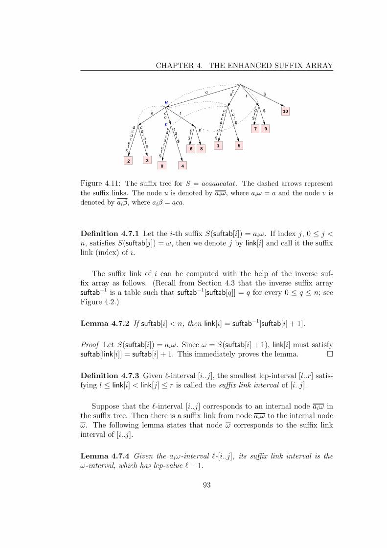
CHAPTER 4. THE ENHANCED SUFFIX ARRAY
at
t$
aaca
at
t$
at
$
$
2
aca
at
t$
ca
at
t$
at
$
$aaca
at
t$
at
t$
ac
ca
a t
a $tu
v
1 5
7 9
3
6 8
0 4
10
Figure 4.11: The suffix tree for S = acaaacatat. The dashed arrows represent
the suffix links. The node u is denoted by aiω, where aiω = a and the node v is
denoted by aiβ, where aiβ = aca.
Definition 4.7.1 Let the i-th suffix S(suftab[i]) = aiω. If index j, 0 ≤ j <n, satisfies S(suftab[j]) = ω, then we denote j by link[i] and call it the suffixlink (index) of i.
The suffix link of i can be computed with the help of the inverse suf-fix array as follows. (Recall from Section 4.3 that the inverse suffix arraysuftab−1 is a table such that suftab−1[suftab[q]] = q for every 0 ≤ q ≤ n; seeFigure 4.2.)
Lemma 4.7.2 If suftab[i] < n, then link[i] = suftab−1[suftab[i] + 1].
Proof Let S(suftab[i]) = aiω. Since ω = S(suftab[i] + 1), link[i] must satisfysuftab[link[i]] = suftab[i] + 1. This immediately proves the lemma. �
Definition 4.7.3 Given `-interval [i..j], the smallest lcp-interval [l..r] satis-fying l ≤ link[i] < link[j] ≤ r is called the suffix link interval of [i..j].
Suppose that the `-interval [i..j] corresponds to an internal node aiω inthe suffix tree. Then there is a suffix link from node aiω to the internal nodeω. The following lemma states that node ω corresponds to the suffix linkinterval of [i..j].
Lemma 4.7.4 Given the aiω-interval `-[i..j], its suffix link interval is theω-interval, which has lcp-value ` − 1.
93
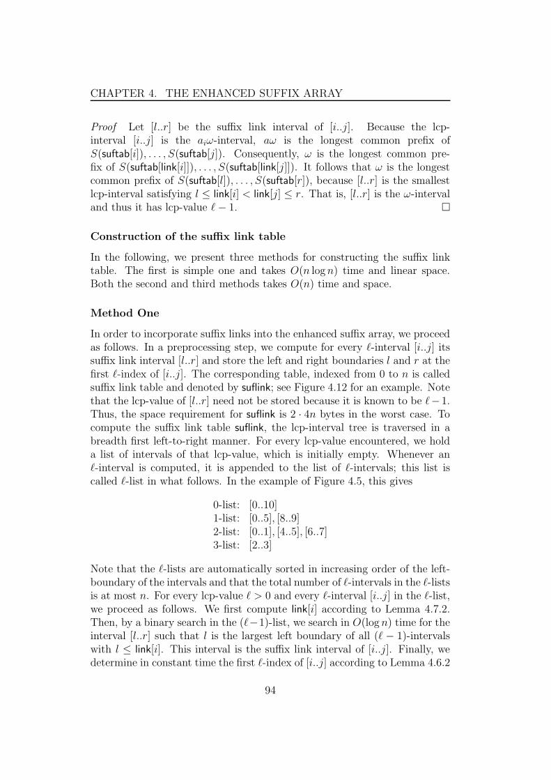
CHAPTER 4. THE ENHANCED SUFFIX ARRAY
Proof Let [l..r] be the suffix link interval of [i..j]. Because the lcp-interval [i..j] is the aiω-interval, aω is the longest common prefix ofS(suftab[i]), . . . , S(suftab[j]). Consequently, ω is the longest common pre-fix of S(suftab[link[i]]), . . . , S(suftab[link[j]]). It follows that ω is the longestcommon prefix of S(suftab[l]), . . . , S(suftab[r]), because [l..r] is the smallestlcp-interval satisfying l ≤ link[i] < link[j] ≤ r. That is, [l..r] is the ω-intervaland thus it has lcp-value ` − 1. �
Construction of the suffix link table
In the following, we present three methods for constructing the suffix linktable. The first is simple one and takes O(n logn) time and linear space.Both the second and third methods takes O(n) time and space.
Method One
In order to incorporate suffix links into the enhanced suffix array, we proceedas follows. In a preprocessing step, we compute for every `-interval [i..j] itssuffix link interval [l..r] and store the left and right boundaries l and r at thefirst `-index of [i..j]. The corresponding table, indexed from 0 to n is calledsuffix link table and denoted by suflink; see Figure 4.12 for an example. Notethat the lcp-value of [l..r] need not be stored because it is known to be `− 1.Thus, the space requirement for suflink is 2 · 4n bytes in the worst case. Tocompute the suffix link table suflink, the lcp-interval tree is traversed in abreadth first left-to-right manner. For every lcp-value encountered, we holda list of intervals of that lcp-value, which is initially empty. Whenever an`-interval is computed, it is appended to the list of `-intervals; this list iscalled `-list in what follows. In the example of Figure 4.5, this gives
0-list: [0..10]1-list: [0..5], [8..9]2-list: [0..1], [4..5], [6..7]3-list: [2..3]
Note that the `-lists are automatically sorted in increasing order of the left-boundary of the intervals and that the total number of `-intervals in the `-listsis at most n. For every lcp-value ` > 0 and every `-interval [i..j] in the `-list,we proceed as follows. We first compute link[i] according to Lemma 4.7.2.Then, by a binary search in the (`−1)-list, we search in O(log n) time for theinterval [l..r] such that l is the largest left boundary of all (` − 1)-intervalswith l ≤ link[i]. This interval is the suffix link interval of [i..j]. Finally, wedetermine in constant time the first `-index of [i..j] according to Lemma 4.6.2
94

CHAPTER 4. THE ENHANCED SUFFIX ARRAY
childtab suflink
i suftab lcptab 1. 2. 3. l r suftab−1 bwttab S(suftab[i])
0 2 0 2 6 2 c aaacatat$
1 3 2 0 5 6 a aacatat$
2 0 1 1 3 4 0 10 0 acaaacatat$
3 4 3 6 7 1 a acatat$
4 6 1 3 5 3 c atat$
5 8 2 8 9 7 t at$
6 1 0 2 7 8 4 a caaacatat$
7 5 2 0 5 8 a catat$
8 7 0 7 9 10 5 a tat$
9 9 1 0 10 9 a t$
10 10 0 9 10 t $
Figure 4.12: Suffix array of the string S = acaaacatat enhanced with the lcp-table,
the child-table, the suffix link table, the inverse suffix array, and the Burrows and
Wheeler table.
and store l and r there. Because there are less than n lcp-intervals and foreach interval the binary search takes O(log n) time, the preprocessing phaserequires O(n log n) time. Table suftab−1 and the `-lists require O(n) space,but they are only used in the preprocessing phase and can be deleted afterthe computation of the suffix link table.
Method 2
Theoretically, it is possible to compute the suffix link intervals in time O(n)via the construction of the suffix tree. But it is also possible to give a lin-ear time algorithm without intermediate construction of the suffix tree. Weachieve this by avoiding the binary search over the `-lists and reducing theproblem of computing the suffix link intervals to the problem of answeringrange minimum queries. In contrast to the previous O(n logn)-time algo-rithm, we store the boundaries i and j of an `-interval [i, j] at every `-index(again, these values can be deleted once the suffix link table suflink is created).
Lemma 4.7.5 Let [i, j] be an `-interval [i, j] and let [l..r] be its suffix linkinterval. Since there is an `-index q with i+1 ≤ q ≤ j, there is also an indexk such that k is an (` − 1)-index of [l..r] and link[i] + 1 ≤ k ≤ link[j].
Proof Follows from the proof of Lemma 4.7.4. �
95
CHAPTER 4. THE ENHANCED SUFFIX ARRAY
Because l ≤ link[i] + 1 ≤ link[j] ≤ r and ` − 1 is the length of the longestcommon prefix of link[i] and link[j], the minimum value of the lcp-table in therange [link[i] + 1..link[j]] is ` − 1. Therefore, one can locate an (` − 1)-indexk of [l..r] with link[i] + 1 ≤ k ≤ link[j] by answering the range minimumquery in the range [link[i] + 1..link[j]]. The range minimum query is definedas follows.
Definition 4.7.6 Let L be an integer-array of size n whose elements are inthe range [0, n − 1]. Let 0 ≤ i < j ≤ n − 1. The range minimum queryrmq(i, j) asks for an index k such that i ≤ k ≤ j and L[k] = min{L[q] | i ≤q ≤ j}.
An rmq can be answered in constant time provided that the array L isappropriately preprocessed. Fortunately, the preprocessing of L requires onlylinear time and space; see [21, 83, 121].
For the computation of suffix link intervals, one solves rmqs for L = lcptab.As in the previous algorithm, the lcp-interval tree is traversed in breadth-firstorder. Thus the `-intervals are processed in ascending order of their lcp-value.Suppose `-interval [i..j] is to be processed and all intervals of lcp-value `− 1have already been processed. First, we store the `-interval boundaries i andj at every `-index of [i..j]. Second, we compute link[i] and link[j] according toLemma 4.7.2, and evaluate k = rmq(link[i]+1, link[j]). k is an (`−1)-index ofthe suffix link interval of [i..j], and thus we can look up the boundaries l andr of this suffix link interval at index k. Finally, we store l and r in the suffixlink table at the first `-index of [i..j]. Because every step in this proceduretakes constant time and space, the overall complexity of computing the suffixlink intervals is O(n).
Method Three
This method constructs the suffix link table in linear time and space withoutusing rmq. In this method, we use a breadth-first traversal to construct thesuffix links in a top-down fashion so that the already constructed suffix linksare used to construct other suffix links. For ease of presentation, we showhow this algorithm works on the suffix tree. Let us first introduce somenotions. Let aiω denote an internal node u of the suffix tree, where theconcatenation of the edge-labels from the root to u spells out the substringaiω, where ai ∈ Σ. Let aiβ denote a child node v of u. Note that the stringaiω is a prefix of aiβ. An example of the nodes u and v is shown in Figure4.11.
Given the suffix tree, a simple way to construct the suffix link of anynode such as aiω is to perform exact pattern matching starting from the root
96
CHAPTER 4. THE ENHANCED SUFFIX ARRAY
to locate the nodes ω. It is clear that the time complexity of this solutionis not linear. However, we can reduce it to O(n) by using the suffix linksconstructed for the parent nodes to avoid searching the suffix tree from theroot every time we traverse a new node.
We traverse the suffix tree in a breadth first order. Assume that thereis a suffix link from aiω to ω, and we are now visiting the node aiβ. Forconstructing the suffix link from aiβ to β, we follow the suffix link of theparent node aiω. It is not difficult to see that the node β is a descendantnode of ω. To reach the node β from ω, one traverses the nodes ω → β0 →· · · → βt → β, t < n, on the path from ω to β. For a node βj, 0 ≤ j ≤ ton this path, the child node βj+1 is determined such that the character
S[|βj| + 1] = a, where a ∈ Σ is the first edge-label on the edge from βj toβj+1. In other words, traversing these nodes does not require to check all theedge-labels on the path. Instead, one checks only the first character of thesubstring annotating the edge from βj to βj+1. That is, the first edge-labelannotating an edge is used to guide the traversal, while the remaining onesare skipped. Once, the node β is reached, a suffix link is constructed fromaiω to ω. The well-informed reader can figure out that the trick of skippingthe edge-labels except the first one is used in the algorithms that constructthe suffix tree in linear time [62]; see also [57]. There, it is proven that everynode is visited a constant number of times, which holds also here becausewe use breadth first traversal. That is, constructing the suffix links given asuffix tree can be done in linear time and space. In the next subsection, wewill see that this trick was also used in the algorithm of Chang and Lawler[37] to perform all suffixes matching in linear time. Simulating this algorithmis straightforward and does not require any additional data structures. Wejust need to allocate space for the suflink table to store the constructed suffixlink and jump to the suffix link intervals. We need also the childtab tableto perform the breadth first traversal of the enhanced suffix array in lineartime. To sum up, Method Three constructs the suffix link table in lineartime and space.
4.7.2 Space efficient computation of MEMs
As an application of the suffix links, we present an algorithm that computesall maximal exact matches by constructing the enhanced suffix array of onlyone sequence and matching the other sequence against it. This has theadvantage of considerably reducing the space requirement for computing thefragments.
97

CHAPTER 4. THE ENHANCED SUFFIX ARRAY
All suffixes matching
Let S1 and S2 be two sequences of lengths n1 and n2 respectively. The keyidea to compute MEMs is to match all the suffixes of S2 against all thoseof S1. Given the enhanced suffix array of S1, a naive solution is to queryall the suffixes of S2 one after another against the enhanced suffix array ofS1. Clearly, this all suffixes matching task requires O((n2)
2) time. However,utilizing the suffix links makes it possible to accomplish this task in timeproportional to the length of S2. Matching all the suffixes of S2 by traversingthe suffix tree using the suffix links was first presented by Chang and Lawler[37] for the purpose of solving the approximate string matching problem insublinear expected time. Here, we call this algorithm all suffixes matching.In the following, we present the enhanced suffix array version of matching allthe suffixes of S2 against S1. Then we show how to employ it for computingfragments of the type maximal exact matches.
First, let us describe the idea of the algorithm on a higher level using thesuffix tree. Recall that we denote an internal node u of a suffix tree with ω ifand only if the concatenation of the edge-labels on the path from the root tou spells out the string ω. For example, let the suffix tree of S1 = acaaacatatbe given. Let cω be an internal node of the suffix tree of S1 and let cβ beits child node (cβ may be a leaf). Examples of such two nodes are shownin Figure 4.13, where ω = a and β = aaacatat$. Moreover, let δ be thesequence of characters labeling the edge between cω and cβ. In the samefigure, δ = aacatat$. Suppose that S2 = caaacag, then matching the firstsuffix of S2 ends at some point on the edge between cω and cβ. The matchedprefix of the first suffix can be written as cωα, where α is a prefix of δ. InFigure 4.13, this point is pointed to with a thick gray arrow, and α = aaca.To match the next suffix of S2 against the suffix tree of S1, one just followsthe suffix link from the node cω to the node ω. This saves matching the first|ω| characters of S2[1..n2] again. Moreover, not all the next |α| characters arematched again. This is made precise as follows. Because the suffix S2[0..n2]has a match of length |cωα|, the suffix S2[1..n2] has a match of length |ωα|.Thus, there is a node β, which is a descendant node of ω (not necessary itschild node), such that (1) α is a prefix of the string that labels the edgeson the path from ω to β, and (2) the string ωα ends at some point on theedge connecting β to its parent node, where |β| ≥ |ωα|. In Figure 4.13, thispoint is pointed to with a thick black arrow. To reach this point startingfrom ω, one traverses the nodes βj, 0 ≤ j ≤ t ≤ n1, on the path from ω toβ. Given the node βj, the node βj+1 is determined such that the characterS2[|βj| + 1] = a, where a ∈ Σ is the first edge-label on the edge connectingβj to βj+1. That is, the first edge-label is used to guide the traversal while
98
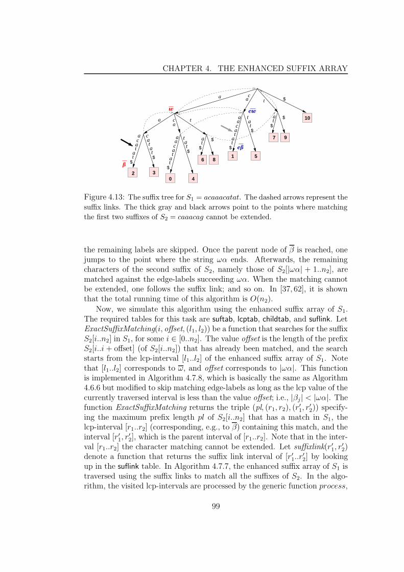
CHAPTER 4. THE ENHANCED SUFFIX ARRAY
at
t$
at
$
$
2
aca
at
t$
ca
at
t$
at
$
$aaca
at
t$
at
t$
ac
ca
aaca
at
t$
a t
a $t
cß
cww
ß1 5
7 9
3
6 8
0 4
10
Figure 4.13: The suffix tree for S1 = acaaacatat. The dashed arrows represent the
suffix links. The thick gray and black arrows point to the points where matching
the first two suffixes of S2 = caaacag cannot be extended.
the remaining labels are skipped. Once the parent node of β is reached, onejumps to the point where the string ωα ends. Afterwards, the remainingcharacters of the second suffix of S2, namely those of S2[|ωα| + 1..n2], arematched against the edge-labels succeeding ωα. When the matching cannotbe extended, one follows the suffix link; and so on. In [37, 62], it is shownthat the total running time of this algorithm is O(n2).
Now, we simulate this algorithm using the enhanced suffix array of S1.The required tables for this task are suftab, lcptab, childtab, and suflink. LetExactSuffixMatching(i, offset, (l1, l2)) be a function that searches for the suffixS2[i..n2] in S1, for some i ∈ [0..n2]. The value offset is the length of the prefixS2[i..i + offset] (of S2[i..n2]) that has already been matched, and the searchstarts from the lcp-interval [l1..l2] of the enhanced suffix array of S1. Notethat [l1..l2] corresponds to ω, and offset corresponds to |ωα|. This functionis implemented in Algorithm 4.7.8, which is basically the same as Algorithm4.6.6 but modified to skip matching edge-labels as long as the lcp value of thecurrently traversed interval is less than the value offset; i.e., |βj| < |ωα|. Thefunction ExactSuffixMatching returns the triple (pl, (r1, r2), (r
′1, r
′2)) specify-
ing the maximum prefix length pl of S2[i..n2] that has a match in S1, thelcp-interval [r1..r2] (corresponding, e.g., to β) containing this match, and theinterval [r′1, r
′2], which is the parent interval of [r1..r2]. Note that in the inter-
val [r1..r2] the character matching cannot be extended. Let suffixlink(r′1, r′2)
denote a function that returns the suffix link interval of [r′1..r′2] by looking
up in the suflink table. In Algorithm 4.7.7, the enhanced suffix array of S1 istraversed using the suffix links to match all the suffixes of S2. In the algo-rithm, the visited lcp-intervals are processed by the generic function process,
99
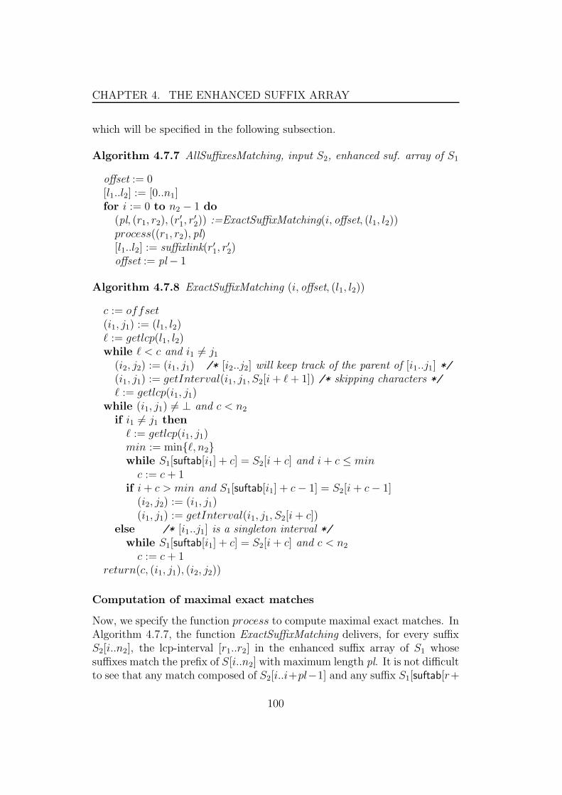
CHAPTER 4. THE ENHANCED SUFFIX ARRAY
which will be specified in the following subsection.
Algorithm 4.7.7 AllSuffixesMatching, input S2, enhanced suf. array of S1
offset := 0[l1..l2] := [0..n1]for i := 0 to n2 − 1 do
(pl, (r1, r2), (r′1, r
′2)) :=ExactSuffixMatching(i, offset, (l1, l2))
process((r1, r2), pl)[l1..l2] := suffixlink(r′1, r
′2)
offset := pl − 1
Algorithm 4.7.8 ExactSuffixMatching (i, offset, (l1, l2))
c := offset(i1, j1) := (l1, l2)` := getlcp(l1, l2)while ` < c and i1 6= j1
(i2, j2) := (i1, j1) /* [i2..j2] will keep track of the parent of [i1..j1] */(i1, j1) := getInterval(i1, j1, S2[i + ` + 1]) /* skipping characters */` := getlcp(i1, j1)
while (i1, j1) 6= ⊥ and c < n2
if i1 6= j1 then` := getlcp(i1, j1)min := min{`, n2}while S1[suftab[i1] + c] = S2[i + c] and i + c ≤ min
c := c + 1if i + c > min and S1[suftab[i1] + c − 1] = S2[i + c − 1]
(i2, j2) := (i1, j1)(i1, j1) := getInterval(i1, j1, S2[i + c])
else /* [i1..j1] is a singleton interval */while S1[suftab[i1] + c] = S2[i + c] and c < n2
c := c + 1return(c, (i1, j1), (i2, j2))
Computation of maximal exact matches
Now, we specify the function process to compute maximal exact matches. InAlgorithm 4.7.7, the function ExactSuffixMatching delivers, for every suffixS2[i..n2], the lcp-interval [r1..r2] in the enhanced suffix array of S1 whosesuffixes match the prefix of S[i..n2] with maximum length pl. It is not difficultto see that any match composed of S2[i..i+pl−1] and any suffix S1[suftab[r+
100

CHAPTER 4. THE ENHANCED SUFFIX ARRAY
1]..suftab[r + 1] + pl − 1], where r1 < r ≤ r2 is a right-maximal exact match.Therefore, in the function process, we perform a Cartesian product betweenS[i..n2] and the suffixes of [r1..r2] to combine right-maximal exact matches,which are specified by the triple (pl, suftab[r], i), where r1 < r ≤ r2. We callthis Cartesian product internal and it is performed only if pl > τ`, where τ`
is a user defined threshold.However, these matches are not all the right-maximal exact matches stem-
ming from the suffix S2[i..n2]. Other right-maximal exact matches that arespecified by (`′, suftab[r′], i), where r′ /∈ [r1..r2], and τ` < `′ < pl, may existand they should also be computed. More precisely, these matches are pro-duced from suffixes outside [r1..r2] belonging to the ancestor lcp-intervals of[r1..r2]. To compute the other ”external” right-maximal exact matches, weperform a second Cartesian product, which we accordingly call it external,as follows. Let the interval [r′1..r
′2] be an ancestor lcp-interval of [r1..r2] of
lcp-value `′ < ` and let suftab[r′] be a suffix belonging to [r′1..r′2] but not
to [r1..r2], then the resulting match with S2[i..n2] is (`′, suftab[r′], i). Thisis because (1) the longest common prefix between any two suffixes suftab[r′]and suftab[r], r ∈ [r1..r2] is `′ (note that lcptab[r′] itself can be larger than `or `′), and (2) S2[i..n2] has a match in [r1..r2] whose length pl > `′′, where `′′
is the lcp-value of the parent interval of [r1..r2].If this algorithm is implemented using the suffix tree, one has to follow
the edges upwards in the tree to process the ancestor intervals. But usingthe enhanced suffix array, the external Cartesian product can be performedin a simpler way. The key idea is the property of the enhanced suffix arraythat the parent intervals are enclosing the child ones. Hence, we can processthe suffixes of the ancestor intervals of [r1..r2] by a linear scanning of theupstream suffixes suftab[r′], where 0 ≤ r′ < r1, lcptab[r′] ≥ τ`, and thedownstream suffixes suftab[r′′], where r2 < r′′ ≤ n1, lcptab[r′′] ≥ τ`. Foran upstream suffix suftab[r′], the resulting match is (`′, suftab[r′], i), where`′ = min{lcptab[r′], . . . , lcptab[r1]} is the match length. The min function isto keep track of the longest common prefix between S2[i..n2] and suftab[r′](noting that lcptab[r′] itself can be larger than ` or `′). The downstreamsuffixes are processed similarly.
Consider the following example. If S2 = acaag and we are given theenhanced suffix array of S1 = acaaacatat shown in Figure 4.12. The firstsuffix of S2 matches the singleton lcp-interval [2..2] with pl = 4. The in-ternal Cartesian product delivers the match (4, 0, 0). The parent interval ofthis singelton interval is the lcp-interval [2..3] of lcp-value 3. The externalCartesian product delivers the match (4, 4, 0), by scanning the downstreamsuffix suftab[3] where min = 3. The parent interval of the lcp-interval [2..3]is [0..5] of lcp value 1. The resulting matches are (1, 3, 0), (1, 2, 0), (1, 6, 0),
101

CHAPTER 4. THE ENHANCED SUFFIX ARRAY
and (1, 8, 0). The first two matches are produced by scanning the upstreamsuffixes suftab[0] and suftab[1], while the last two ones are produced by scan-ning the downstream suffixes suftab[4] and suftab[5]. In both cases, we havemin = 1.
The left-maximality of the right-maximal exact matches, computed byeither Cartesian product, can be checked upon reporting the matches. Hence,the running time of computing maximal exact matching using this algorithmis O(n2 + zr), where zr is the number of right-maximal exact matches.
4.8 Implementation details
In this section, we present implementation details of the enhanced suffix ar-rays. We show how to further reduce the space requirement for each tableenhancing the suffix array using a set of programming tricks. Our experi-ments, presented in the next section, show that this space reduction entails noloss of performance for genomic data, albeit the worst case time complexitiesof some algorithms may be affected.
4.8.1 The lcp-table
It has already been mentioned that the lcp-table requires 4n bytes in theworst case. In practice, however, the lcp-table can be implemented in littlemore than n bytes. More precisely, we store most of the values of tablelcptab in a table lcptab1 using n bytes. That is, for any i ∈ [1, n], lcptab1[i] =max{255, lcptab[i]}. There are usually only few entries in lcptab that arelarger than or equal to 255. For instance, the enhanced suffix array of thebacterial genome E. coli , which is of length 4,639,221, has approximately1.5% of the lcptab entries that are larger than or equal to 255. For yeast,which is of length 12,156,300, the percentage ≈ 4.36%. To access theseefficiently, we store them in an extra table llvtab. This contains all pairs(i, lcptab[i]) such that lcptab[i] ≥ 255, ordered by the first component. Eachentry in llvtab requires 8 bytes. If lcptab1[i] = 255, then the correct value oflcptab is found in llvtab. If we scan the values in lcptab1 in consecutive order(this holds for applications based on properties of the enhanced suffix arrayand applications based on bottom-up traversal of the enhanced suffix array)and find a value 255, then we access the correct value in lcptab in the nextentry of table llvtab. If we access the values in lcptab1 in arbitrary order andfind a value 255 at index i, then we perform a binary search in llvtab using ias the key. This delivers lcptab[i] in O(log2 |llvtab|) time.
102
CHAPTER 4. THE ENHANCED SUFFIX ARRAY
4.8.2 The child-table
As the lcp-table, the child-table requires 4n bytes but in practice it can bestored in n bytes without loss of performance. To achieve this goal, we storerelative indices in childtab. For example, if j = childtab[i].next`Index, thenwe store j−i. The relative indices are almost always smaller than 255. Hencewe use only one byte for storing a value of table childtab. The values ≥ 255are not stored. Instead, if we encounter the value 255 in childtab, then weuse a function that is equivalent to getInterval , except that it determines achild interval by a binary search, similar to the algorithm of [100, page 937].Consequently, instead of 4 bytes per entry of the child-table, only 1 byte isneeded. The overall space consumption for tables suftab, lcptab, and childtab
is thus only 6n bytes.For a given parameter d, we additionally use an extra bucket table bcktabd.
This table stores for each substring w of length d the smallest integer i, suchthat S[suftab[i] . . . suftab[i] + d − 1] = w. In other words, it is a hash tablewhose hashing function, for each w = S[suftab[i] . . . suftab[i] + d − 1], is
x =
l+d−1∑
i=l
|Ψ|d−1T (S[i])
where x is an integer value representing an index of the hash table, Ψ isthe alphabet plus an additional dummy character, T (S[i]) is a function thatmaps each character in the alphabet to a number in the range [0 . . . |Σ|].The dummy character is used to access the prefixes of w. That is, for prefixw′ of length d′, we append d − d′ dummy characters and then compute thehash function. It is easy to see that two successive non-empty entries ofthis table identifies an lcp-interval of lcp-value d′ ≤ d corresponding to theprefixes of S[l..l + d − 1]. In this way we can answer small queries of lengthd′ ≤ d in time O(d′). For larger queries, this bucket table allows us to locatethe interval containing the d-character prefix P [0..d − 1] of the query P inconstant time. Then our algorithm, which searches for the pattern P in S,starts with this interval instead of the interval [0..n]. The value d is chosento be the maximal value such that table bcktabd never requires more than nbytes. The advantage of this hybrid method is that only a small part of thesuffix array is actually accessed. Moreover, we rarely access the values 255in childtab.
4.8.3 The suffix link table
Here, we also make use of the bucket table bcktabd to store the suffix linktable in 2n bytes instead of 8n bytes. Suppose we want to compute the suffix
103
CHAPTER 4. THE ENHANCED SUFFIX ARRAY
link interval of some `-interval [i..j]. If ` ≤ d + 1, then this can be done inconstant time by some integer arithmetic and looking up appropriate valuesin table bcktabd. For lcp-intervals whose lcp-value ` > d + 1, we store in thesuflink table the left and right boundaries of its suffix link interval relativeto the ancestor d-interval of the suffix link interval. This d-interval can beaccessed in constant time by looking up in bcktabd. That is, to computethe suffix link interval of some `-interval, where ` > d + 1, we first locatethe d-interval of the suffix link interval by looking up in bcktabd. Then, weaccess suflink table as described at the beginning of Section 4.7.1 to obtainthe relative left and right boundaries. Storing relative positions in the fieldsof the suflink table allows to reduce the corresponding space to 2 bytes perentry. For relative positions larger than 255, the suffix link intervals arelocated using binary search. Altogether, the suffix link table suflink requiresonly 2n bytes in our implementation.
4.9 Experimental results
For our experiments, we collected a set of files of different sizes and types:
E. coli : The complete genome of the bacterium Escherichia coli, strain K12.This is a DNA sequence of length 4,639,221. The alphabet size is 4.
Yeast : The complete genome of the baker’s yeast Saccharomyces cerevisiae,i.e., a DNA sequence of length 12,156,300 bp. The alphabet size is 4.
Hs21 : The complete sequence of the human chromosome 21. The length is33,917,895 bp. The alphabet size is 4.
Swissprot : The complete collection of protein sequences from the Swissprotdatabase (release 38). The total size of all sequences is 29,165,964character. The alphabet size is 20.
Shaks: A collection of the complete works of William Shakespeare. Thetotal size is 5,582,655 bytes. The alphabet size is 92.
In addition we collected four different pairs of similar genomes:
Streptococuss 2: The complete genomes of two strains of the bacteriaStreptococcus pneumoniae (length 2,160,837 and 2,038,615 bp).
E. coli 2: E. coli (see above) and the complete genome of a different strainof this bacterium (E. coli O157:H7, length 5,528,445).
104

CHAPTER 4. THE ENHANCED SUFFIX ARRAY
Yeast 2: Yeast (see above) and the complete genome of a different kind ofyeast (S. pombe, length 12,534,386 bp).
Human 2: Hs21 (see above) and the human chromosome 22 Hs22 (length33,821,705 bp).
Prior to all computations described below, we constructed the enhanced suffixarray for all input sequences. Each of the tables comprising the index isstored on a different file. The construction was done by a program that isbased on the suffix sorting algorithm of [26]. This program uses about 50%less space than the best programs constructing suffix trees (see below). Theenhanced suffix array is constructed in about the same time as the suffix tree.(The comparison of the suffix array and suffix tree construction algorithmsis beyond the scope of this thesis.) Because both suffix tree and enhancedsuffix array are indexing structures that are usually constructed only oncefor a genomic sequence, we focus on the applications based on these datastructures and report the running times excluding the time for constructingthe suffix tree and the enhanced suffix array. All programs based on suffixarrays use memory mapping to access the enhanced suffix array from thedifferent files. Of course, a file is mapped into main memory only if the tableit stores is required for the particular algorithm; see Table 4.8.
The running times reported here are for a SUN-Sparc computer equippedwith 32 gigabytes RAM and a 950 Mhz CPU. For our tests, we only neededat most 3165 megabytes of memory.
4.9.1 Algorithms based on properties of enhanced suf-
fix arrays
Computing supermaximal repeats
In our first experiment, we ran our program esasupermax that computessupermaximal repeats. This program implements the algorithm described inSection 4.4.3, which is based only on the properties of enhanced suffix arrays.We ran also the strmat-package of [84] which is based on the suffix tree andimplements a more complicated algorithm [62] than ours for the same task.Table 4.2 shows the running times of our program applied for the detection ofsupermaximal repeats to E. coli , Yeast , and Hs21 . The space requirement isindependent of `, and it is 31, 72, and 195 megabytes for E. coli , Yeast , andHs21 respectively. The running time of esasupermax is almost independentof the minimal length of the supermaximal repeats computed. We refer thisto the improved cache behavior achieved by the linear scanning of the tablessuftab, lcptab, and bwttab. (The usage of bwttab avoided us random access to
105
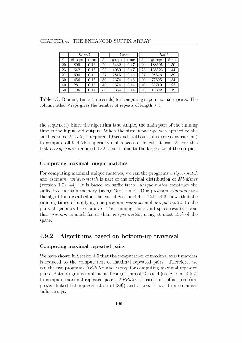
CHAPTER 4. THE ENHANCED SUFFIX ARRAY
E. coli
` # reps time20 899 0.1623 642 0.1527 500 0.1530 456 0.1540 281 0.1550 196 0.14
Yeast
` #reps time20 6432 0.4723 4069 0.4727 2813 0.4530 2374 0.4640 1674 0.4450 1354 0.44
Hs21
` # reps time20 188695 1.5023 138523 1.4427 98346 1.3930 77695 1.3440 35719 1.2350 16392 1.19
Table 4.2: Running times (in seconds) for computing supermaximal repeats. The
column titled #reps gives the number of repeats of length ≥ `.
the sequence.) Since the algorithm is so simple, the main part of the runningtime is the input and output. When the strmat-package was applied to thesmall genome E. coli , it required 19 second (without suffix tree construction)to compute all 944,546 supermaximal repeats of length at least 2. For thistask esasupermax required 0.82 seconds due to the large size of the output.
Computing maximal unique matches
For computing maximal unique matches, we ran the programs unique-matchand esamum. unique-match is part of the original distribution of MUMmer(version 1.0) [44]. It is based on suffix trees. unique-match construct thesuffix tree in main memory (using O(n) time). Our program esamum usesthe algorithm described at the end of Section 4.4.4. Table 4.3 shows that therunning times of applying our program esamum and unique-match to thepairs of genomes listed above. The running times and space results revealthat esamum is much faster than unique-match, using at most 15% of thespace.
4.9.2 Algorithms based on bottom-up traversal
Computing maximal repeated pairs
We have shown in Section 4.5 that the computation of maximal exact matchesis reduced to the computation of maximal repeated pairs. Therefore, weran the two programs REPuter and esarep for computing maximal repeatedpairs. Both programs implement the algorithm of Gusfield (see Section 4.5.2)to compute maximal repeated pairs. REPuter is based on suffix trees (im-proved linked list representation of [89]) and esarep is based on enhancedsuffix arrays.
106

CHAPTER 4. THE ENHANCED SUFFIX ARRAY
unique-match esamum
genome pair total size #MUMs time space time space
Streptococuss 2 4,199,453 6613 9.0 196 0.33 30E. coli 2 10,107,957 10817 30.7 472 0.69 62Yeast 2 24,690,687 2536 118.2 1154 0.66 144Human 2 67,739,601 217014 430.1 3165 2.34 389
Table 4.3: Running times (in seconds) and space consumption (in megabytes) for
computing MUMs of length ≥ 20. The column titled #MUMs gives the number of
MUMs. The time given for unique-match does not include suffix tree construction.
esamum reads the enhanced suffix array from different files via memory mapping.
The comparison of esarep and REPuter underlines the advantages of theenhanced suffix array over the suffix tree. Table 4.4 shows that esarep usedabout halve of the space of REPuter . It also shows that esarep is 4-5 timesfaster than REPuter . This is due to the improved cache behavior achievedby the linear scanning of the tables suftab, lcptab, and bwttab.
Computing tandem repeats
For computing tandem repeats, we have implemented the three algorithmsOBA, iOBA, and BFA. and 4.6.2. OBA is an implementation of the optimizedbasic algorithm Algorithm 4.5.9, and iOBA incorporates our improvementsdescribed in Algorithm 4.5.11. Both algorithms are explained in Subsection4.5.5. BFA implements the brute force algorithm described in Subsection4.6.2. Table 4.5 summarizes the results of these experiments.
The most surprising result of our experiments is the superior runningtime of the brute force algorithm to compute branching tandem repeats.BFA is always faster than the other two algorithms. iOBA is faster thanOBA if ` ≤ 11, and slightly slower if ` ≥ 14. This is due to the fact that theadditional access to the text, which is necessary to find the appropriate childinterval [ia..ja], outweighs the efficiency gain due to the reduced number ofsuffix checks.
We have also measured the running time of a program implementing thelinear time algorithm of [63] to compute all tandem repeats. It is part of thestrmat-package. For E. coli the program needs about 21 second (withoutsuffix tree construction) and 490 MB main memory to deliver all tandemrepeats of length at least 2. The linear time algorithm of [86] takes 4.7 secondusing 63 MB of main memory. For the same task our fastest program BFA(with an additional post processing step to compute non-branching tandemrepeats from branching tandem repeats) requires 1.7 sec and 27 MB of main
107
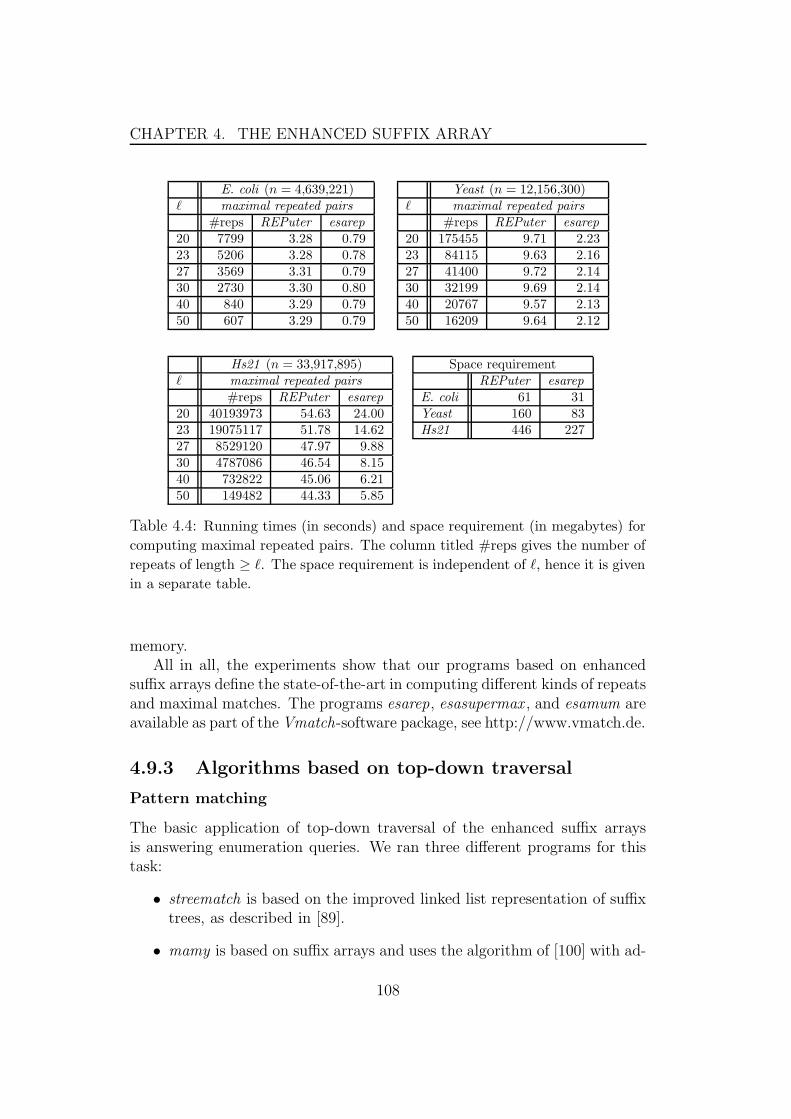
CHAPTER 4. THE ENHANCED SUFFIX ARRAY
E. coli (n = 4,639,221)` maximal repeated pairs
#reps REPuter esarep
20 7799 3.28 0.7923 5206 3.28 0.7827 3569 3.31 0.7930 2730 3.30 0.8040 840 3.29 0.7950 607 3.29 0.79
Yeast (n = 12,156,300)` maximal repeated pairs
#reps REPuter esarep
20 175455 9.71 2.2323 84115 9.63 2.1627 41400 9.72 2.1430 32199 9.69 2.1440 20767 9.57 2.1350 16209 9.64 2.12
Hs21 (n = 33,917,895)` maximal repeated pairs
#reps REPuter esarep
20 40193973 54.63 24.0023 19075117 51.78 14.6227 8529120 47.97 9.8830 4787086 46.54 8.1540 732822 45.06 6.2150 149482 44.33 5.85
Space requirementREPuter esarep
E. coli 61 31Yeast 160 83Hs21 446 227
Table 4.4: Running times (in seconds) and space requirement (in megabytes) for
computing maximal repeated pairs. The column titled #reps gives the number of
repeats of length ≥ `. The space requirement is independent of `, hence it is given
in a separate table.
memory.All in all, the experiments show that our programs based on enhanced
suffix arrays define the state-of-the-art in computing different kinds of repeatsand maximal matches. The programs esarep, esasupermax , and esamum areavailable as part of the Vmatch-software package, see http://www.vmatch.de.
4.9.3 Algorithms based on top-down traversal
Pattern matching
The basic application of top-down traversal of the enhanced suffix arraysis answering enumeration queries. We ran three different programs for thistask:
• streematch is based on the improved linked list representation of suffixtrees, as described in [89].
• mamy is based on suffix arrays and uses the algorithm of [100] with ad-
108
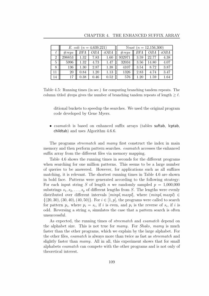
CHAPTER 4. THE ENHANCED SUFFIX ARRAY
E. coli (n = 4,639,221)
` #reps BFA OBA iOBA
2 298853 1.32 7.83 1.60
5 5996 1.32 4.73 1.47
8 136 1.30 2.87 1.38
11 20 0.84 1.20 1.13
14 17 0.38 0.46 0.52
Yeast (n = 12,156,300)
#reps BFA OBA iOBA
932971 3.59 22.77 4.38
32034 3.56 14.80 4.07
4107 3.54 8.72 3.87
1326 2.83 4.74 3.47
576 1.20 1.59 1.64
Table 4.5: Running times (in sec.) for computing branching tandem repeats. The
column titled #reps gives the number of branching tandem repeats of length ≥ `.
ditional buckets to speedup the searches. We used the original programcode developed by Gene Myers.
• esamatch is based on enhanced suffix arrays (tables suftab, lcptab,childtab) and uses Algorithm 4.6.6.
The programs streematch and mamy first construct the index in mainmemory and then perform pattern searches. esamatch accesses the enhancedsuffix array from the different files via memory mapping.
Table 4.6 shows the running times in seconds for the different programswhen searching for one million patterns. This seems to be a large numberof queries to be answered. However, for applications such as all suffixesmatching, it is relevant. The shortest running times in Table 4.6 are shownin bold face. Patterns were generated according to the following strategy:For each input string S of length n we randomly sampled p = 1,000,000substrings s1, s2, . . . , sp of different lengths from S. The lengths were evenlydistributed over different intervals [minpl,maxpl], where (minpl,maxpl) ∈{(20, 30), (30, 40), (40, 50)}. For i ∈ [1, p], the programs were called to searchfor pattern pi, where pi = si, if i is even, and pi is the reverse of si, if i isodd. Reversing a string si simulates the case that a pattern search is oftenunsuccessful.
As expected, the running times of streematch and esamatch depend onthe alphabet size. This is not true for mamy . For Shaks, mamy is muchfaster than the other programs, which we explain by the large alphabet. Forthe other files, esamatch is always more than twice as fast as streematch andslightly faster than mamy . All in all, this experiment shows that for smallalphabets esamatch can compete with the other programs and is not only oftheoretical interest.
109

CHAPTER 4. THE ENHANCED SUFFIX ARRAY
time for minpl = 20,maxpl = 30file stree mamy esa
E. coli 9.47 5.56 4.48
Yeast 12.42 8.26 5.37
Hs21 20.15 12.50 7.23
Swissprot 41.78 9.55 6.22
Shaks 15.61 4.29 72.44
time for minpl = 30,maxpl = 40file stree mamy esa
E. coli 9.63 5.70 4.69
Yeast 12.56 8.46 5.80
Hs21 20.43 12.69 7.30
Swissprot 40.80 10.09 6.25
Shaks 15.78 4.37 66.60
time for minpl = 40,maxpl = 50file stree mamy esa
E. coli 9.86 5.87 4.85
Yeast 13.34 8.63 5.74
Hs21 21.22 12.88 7.61
Swissprot 42.96 9.83 6.39
Shaks 15.88 4.49 67.16
space requirementfile stree mamy esa
E. coli 56 40 47Yeast 146 106 120Hs21 407 296 327Swissprot 320 288 281Shaks 52 48 60
Table 4.6: Running times (in seconds) and space requirement (in megabytes) for
one million enumeration queries searching for exact patterns in the input strings.
minpl and maxpl are the minimal and maximal size of the patterns searched for.
Searching for all minimal unique substrings
We implemented the breadth first traversal algorithm of Section 4.6.2 tofind all minimal unique substrings. We applied it to E. coli and Yeast .For E. coli our program computed three minimal unique substrings, each oflength 7. It processed 11,392 lcp-intervals (0.38% of all 2,978,098 lcp-intervalsin the corresponding lcp-interval tree). For Yeast our program computed383 minimal unique substrings, each of length 9. It processed 92,863 lcp-intervals (1.2% of all 7,904,703 lcp-intervals in the corresponding lcp-intervaltree). To demonstrate the efficiency of our solution to the minimal uniquesubstring problem, we implemented a straightforward method to solve thesame problem by enumerating all lcp-intervals. The straightforward methodwas 5 times slower than ours in case of E. coli and 9 times slower in case ofYeast .
4.9.4 Algorithms for traversals using suffix links
For our final experiment, we applied two programs that perform all suffixesmatching, the task described in Section 4.7.2. The first program streemsis based on the improved linked list implementation of suffix trees, whileour program esams uses the enhanced suffix arrays as described in Section4.7.2. The experiments (Table 4.7) show a trade-off between time and space
110
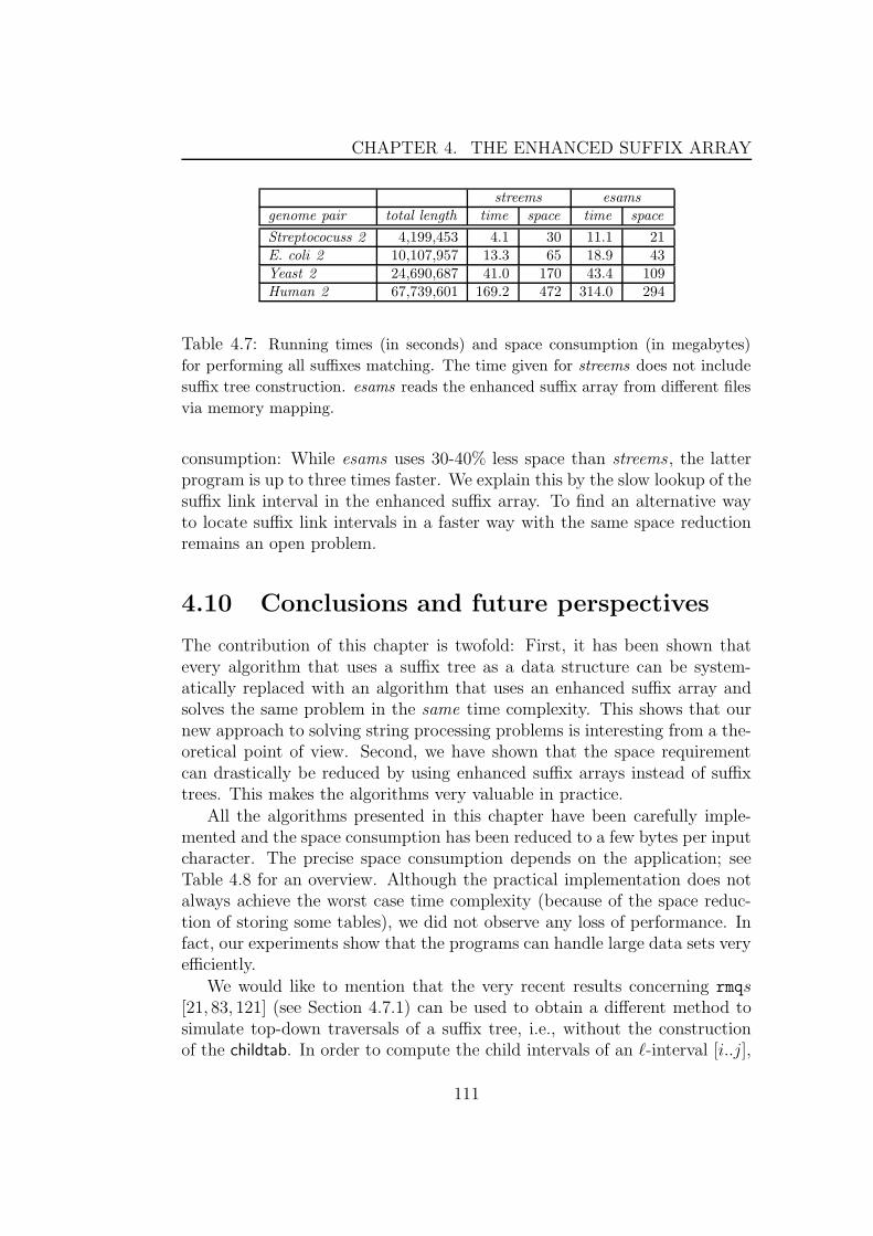
CHAPTER 4. THE ENHANCED SUFFIX ARRAY
streems esams
genome pair total length time space time space
Streptococuss 2 4,199,453 4.1 30 11.1 21E. coli 2 10,107,957 13.3 65 18.9 43Yeast 2 24,690,687 41.0 170 43.4 109Human 2 67,739,601 169.2 472 314.0 294
Table 4.7: Running times (in seconds) and space consumption (in megabytes)
for performing all suffixes matching. The time given for streems does not include
suffix tree construction. esams reads the enhanced suffix array from different files
via memory mapping.
consumption: While esams uses 30-40% less space than streems, the latterprogram is up to three times faster. We explain this by the slow lookup of thesuffix link interval in the enhanced suffix array. To find an alternative wayto locate suffix link intervals in a faster way with the same space reductionremains an open problem.
4.10 Conclusions and future perspectives
The contribution of this chapter is twofold: First, it has been shown thatevery algorithm that uses a suffix tree as a data structure can be system-atically replaced with an algorithm that uses an enhanced suffix array andsolves the same problem in the same time complexity. This shows that ournew approach to solving string processing problems is interesting from a the-oretical point of view. Second, we have shown that the space requirementcan drastically be reduced by using enhanced suffix arrays instead of suffixtrees. This makes the algorithms very valuable in practice.
All the algorithms presented in this chapter have been carefully imple-mented and the space consumption has been reduced to a few bytes per inputcharacter. The precise space consumption depends on the application; seeTable 4.8 for an overview. Although the practical implementation does notalways achieve the worst case time complexity (because of the space reduc-tion of storing some tables), we did not observe any loss of performance. Infact, our experiments show that the programs can handle large data sets veryefficiently.
We would like to mention that the very recent results concerning rmqs[21, 83, 121] (see Section 4.7.1) can be used to obtain a different method tosimulate top-down traversals of a suffix tree, i.e., without the constructionof the childtab. In order to compute the child intervals of an `-interval [i..j],
111

CHAPTER 4. THE ENHANCED SUFFIX ARRAY
Program name application
esasupermax supermaximal repeatsesamum maximal unique matchesesarep maximal repeated pairsmultimat maximal (multiple) exact matchesZiv-Lempel Ziv-Lempel decompositionOBA tandem repeats, optimized algorithmiOBA tandem repeats, improved optimized algorithmBFA tandem repeats, brute-force algorithmesamatch exact pattern matchingesams all suffixes matching
Enhanced suffix array
Application suftab suftab−1 lcptab childtab suflink S bwttab
4n bytes 4n bytes n bytes n bytes 2n bytes
esasupermax√ √ √
esamum√ √ √
esarep√ √ √
multimat√ √ √
Ziv-Lempel√ √
OBA, iOBA√ √ √
esamatch√ √ √ √
esasus√ √ √
BFA√ √ √ √
esams√ √ √ √ √
Table 4.8: Above: Program names and the respective applications. Below: Sum-
mary of the tables required for the applications mentioned in the chapter. Both S
and bwttab require n log |Σ| bits. The program esamum, for example, requires an
enhanced suffix array consisting of the tables suftab, lcptab, and bwttab.
it suffices to compute the `-indices of [i..j]; see Lemma 4.6.1. By Definition4.4.1, the `-indices i1 < i2 < · · · < ik of [i..j] are the indices with minimumlcp-value in the range [i + 1..j]. Suppose that every rmq returns the firstindex k such that lcptab[k] is minimum in the given range (according to[83], one such rmq can be answered in constant time). Then the `-indicesof [i..j] can be found by successively computing i1 := rmq(i + 1, j), i2 :=rmq(i1 + 1, j), . . . , ik := rmq(ik−1 + 1, j), until rmq(ik + 1, j) returns a value qsuch that lcptab[q] 6= `. Future work will show whether this approach is alsoof practical interest.
Computing maximal exact matches using the all suffixes matching algo-rithm significantly reduces the space required for this task. A theoreticalshortcoming of this method is that its running time is proportional to the
112

CHAPTER 4. THE ENHANCED SUFFIX ARRAY
number of right maximal exact matches, which is higher than the number ofmaximal exact matches. It is, therefore, an interesting problem to reduce itsrunning time to be proportional to the number of maximal exact matches,and not to the number of right maximal exact matches. Moreover, it is anopen problem to develop an algorithm that computes multiMEMs using theindex of a single sequence and matching the other sequences against it, i.e.,to generalize the all suffixes matching algorithm for k sequences. It would bealso practical to incorporate the notions of rare and infrequent multiMEMsin this algorithm.
Clearly, it would be desirable to further reduce the space requirement ofthe suffix array. Recently, interesting results in this direction have been ob-tained. The most notable ones are the compressed suffix array introduced byGrossi and Vitter [60] and the so-called opportunistic data structure devisedby Ferragina and Manzini [52]. More recently, Hon and Sadakane [69] andSadakane [121] showed that compressed suffix arrays can be used to solvestring processing tasks like computing all MUMs of two sequences. However,to develop a software tool based on compressed suffix arrays that can com-pete, in practice, with our enhanced suffix arrays remains an open problem.Moreover, a systematic approach like ours has not yet been developed forcompressed suffix arrays.
113

Chapter 5
Chaining Algorithms
5.1 Introduction
Chaining algorithms became the technique of choice in software tools thatrely on the anchor based strategy for comparing genomes. As mentioned inChapter 3, the anchor-based strategy is composed of three phases:
1. Computation of fragments (segments in the genomes that are similar).
2. Computation of a highest-scoring global chain or a set of significantlocal chains of colinear non-overlapping fragments. The fragments of achain are the anchors that form the basis of the alignment.
3. Alignment of the regions within and surrounding the anchors on thecharacter level.
This chapter deals with algorithms for solving the combinatorial chainingproblem of the second phase, i.e., finding a highest-scoring global chain or aset of significant local chains of colinear non-overlapping fragments. We alsoaddress several variations of the chaining algorithms. These variations extendthe range of application to solve various comparative genomics problems.
This chapter is organized as follows. In Section 5.2, we begin with intro-ducing the basic concepts and definitions. In Section 5.3, the global chainingproblem is introduced. For clarity of proposition, we solve the global chainingproblem in stages distributed over many sections. In Section 5.4, we presenta global chaining algorithm only for two genomes. The presented algorithmneglects the gap costs, i.e., gaps between the fragments are not penalizedat all. Then in Section 5.5, we outline the extension of this global chainingalgorithm to the higher-dimensional case. This extension makes it possibleto compare multiple genomes simultaneously. Afterwards, the algorithms are
115
CHAPTER 5. CHAINING ALGORITHMS
modified in Section 5.6 in two steps so that they can deal with certain gapcosts.
In Section 5.7, we present the local chaining problem, which is a variationof the global chaining problem. The results of this section provides a solutionto the problem of automatically finding local regions of similarity in largegenomic DNA sequences. In Section 5.8, we present further variations of thechaining problem such as the inclusion of gap constraints and cDNA/ESTmapping.
In Section 5.9, we discuss two related problems: The first is the onedimensional chaining problem that is used for (1) finding the maximumcoverage of one genome w.r.t. the other, and (2) computing the transfor-mation distance between two genomes. The second is the maximum weightindependent set problem that is used for determining the relative degrees ofcompletion of two sequencing projects.
Finally, Section 5.10 summarizes the results obtained in this chapter anddiscusses the open problems and future work.
5.2 Basic concepts and definitions
Let us first recall the definition of a fragment. Let Si[1 . . . ni], 1 ≤ i ≤ k,denote a string of length |Si| = ni. In our application, Si is the DNA sequenceof a genome. Si[li . . . hi] is the substring of Si starting at position li andending at position hi. A fragment f consists of two pairs beg(f)= (l1, . . . , lk)and end(f)= (h1, . . . , hk) such that the substrings (henceforth also calledsegments) S1[l1 . . . h1], . . . , Sk[lk . . . hk] are “similar”. We call a fragmentexact, if it is composed of exact matches, i.e., S1[l1 . . . h1] = S2[l2 . . . h2] =. . . = Sk[lk . . . hk]. Examples of exact fragments are the exact k-mers asused in BLASTZ [125], maximal exact matches MEMs as used in AVID[28], the maximal multiple exact matches multiMEMs as used in MGA [68],the maximal unique matches MUMs as used in MUMmer [44, 45], and themaximal multiple unique matches multiMUMs as used in EMAGEN [46]and Mauve [43]. We call a fragment non-exact, if it is composed of non-exactmatches, i.e., S1[l1 . . . h1] ≈ S2[l2 . . . h2] ≈ · · · ≈ Sk[lk . . . hk]. Examples, ofnon-exact fragments are the non-exact k-mers as used in the recent versionof BLASTZ [124], and the extended seeds of GLASS [19]. We stress that ourchaining algorithms can handle any kind of fragments.
A fragment f of k genomes can be represented by a hyper-rectangle in Rk
with the two extreme corner points beg(f) and end(f), where each coordinateof the points is a non-negative integer (consequently, the words number ofgenomes and dimension will be used synonymously in what follows). To
116
CHAPTER 5. CHAINING ALGORITHMS
fix notation, we recall the following concepts. For any point p ∈ Rk, let
p.x1, p.x2, . . . p.xk denote its coordinates. We will also sometimes use p.xand p.y instead of p.x1 and p.x2 for points p ∈ R
2. A hyper-rectangle (calledhyper-rectangular domain in [118]) is the Cartesian product of intervals ondistinct coordinate axes. A hyper-rectangle [l1 . . . h1] × [l2 . . . h2] × · · · ×[lk . . . hk] (with li < hi for all 1 ≤ i ≤ k) will here be denoted by R(p, q),where p = (l1, . . . , lk) and q = (h1, . . . , hk). Figure 5.1 shows fragments fortwo sequences (two dimensions) and their rectangular representation in twodimensional plot.
With every fragment f , we associate a positive weight f.weight ∈ R.This weight can, for example, be the length of the fragment (in case ofexact fragments) or its statistical significance. In what follows, we will oftenidentify the point beg(f) or end(f) with the fragment f (every point canbe annotated with a tag that identifies the fragment it stems from). Forexample, if we speak about the weight of a point beg(f) or end(f), we meanthe weight of the fragment f .
For ease of presentation, we consider the points 0 = (0, . . . , 0), the origin,and t = (|S1| + 1, . . . , |Sk| + 1), the terminus, as fragments with weight 0.For these fragments, we define beg(0) = ⊥, end(0) = 0, beg(t) = t, andend(t) = ⊥.
Two fragments are colinear if the order of their respective segments is thesame in both genomes. In the pictorial representation of Figure 5.1(a), twofragments are colinear if the lines connecting their segments are non-crossing(in Figure 5.1, for example, the fragments 2 and 3 are colinear, while 1 and6 are not). Two fragments overlap if their segments overlap in one of thegenomes (in Figure 5.1, for example, the fragments 1 and 2 are overlapping,while 2 and 3 are non-overlapping). The non-overlapping and colinearityrelations between two fragments can be defined formally as follows.
Definition 5.2.1 The binary relation � is defined on the set of fragmentsby f � f ′ if and only if end(f).xi < beg(f ′).xi for all 1 ≤ i ≤ k. If f � f ′,then they are colinear and non-overlapping, and we say that f precedes f ′.
Note that 0 � f � t for every fragment f with f 6= 0 and f 6= t.
Definition 5.2.2 A chain of colinear non-overlapping fragments (or chainfor short) is a sequence of fragments f1, f2, . . . , f` such that fi � fi+1 for all1 ≤ i < `. The score of C is
score(C) =∑
i=1
fi.weight −`−1∑
i=1
g(fi+1, fi)
117
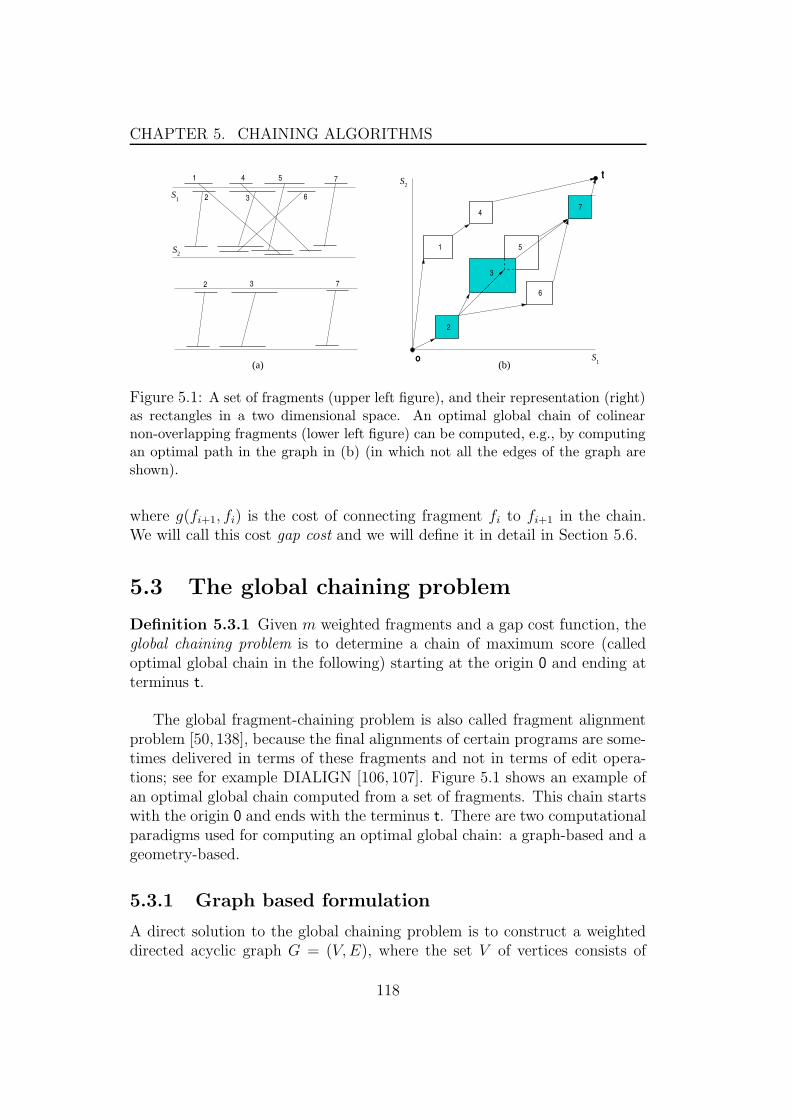
CHAPTER 5. CHAINING ALGORITHMS
(b)(a)
t
o
6
5
4
3
632
1 7542S
S
2S
1S
732
1
1
2
7
Figure 5.1: A set of fragments (upper left figure), and their representation (right)as rectangles in a two dimensional space. An optimal global chain of colinearnon-overlapping fragments (lower left figure) can be computed, e.g., by computingan optimal path in the graph in (b) (in which not all the edges of the graph areshown).
where g(fi+1, fi) is the cost of connecting fragment fi to fi+1 in the chain.We will call this cost gap cost and we will define it in detail in Section 5.6.
5.3 The global chaining problem
Definition 5.3.1 Given m weighted fragments and a gap cost function, theglobal chaining problem is to determine a chain of maximum score (calledoptimal global chain in the following) starting at the origin 0 and ending atterminus t.
The global fragment-chaining problem is also called fragment alignmentproblem [50, 138], because the final alignments of certain programs are some-times delivered in terms of these fragments and not in terms of edit opera-tions; see for example DIALIGN [106, 107]. Figure 5.1 shows an example ofan optimal global chain computed from a set of fragments. This chain startswith the origin 0 and ends with the terminus t. There are two computationalparadigms used for computing an optimal global chain: a graph-based and ageometry-based.
5.3.1 Graph based formulation
A direct solution to the global chaining problem is to construct a weighteddirected acyclic graph G = (V, E), where the set V of vertices consists of
118

CHAPTER 5. CHAINING ALGORITHMS
all fragments (including 0 and t) and the set of edges E is characterized asfollows: There is an edge f → f ′ with weight f ′.weight − g(f ′, f) if f � f ′;see Figure 5.1(b). An optimal global chain of fragments corresponds to apath of maximum score from vertex 0 to vertex t in the graph. Because thegraph is acyclic, such a path can be computed as follows. Let f ′.score bedefined as the maximum score of all chains starting at 0 and ending at f ′.f ′.score can be expressed by the recurrence: 0.score = 0 and
f ′.score = f ′.weight + max{f.score − g(f ′, f) : f � f ′} (5.1)
A dynamic programming algorithm based on this recurrence takes O(|V | +|E|) time provided that computing gap costs takes constant time. Because|V | + |E| ∈ O(m2), computing an optimal global chain takes quadratic timeand linear space; see [40, 94]. This graph-based solution works for any numberof genomes and for any kind of gap costs. It had been proposed as a practicalapproach (compared to the standard dynamic programming) for aligningbiological sequences, first for two sequences by Wilbur and Lipman [138] andfor multiple sequences by Sobel and Martinez [128]. Later, this formulationwas used in the first version of MGA [68] for computing an optimal globalchain, but without considering gap costs. More recently, the software toolEMAGEN used the analogous trapezoid graph formulation [42] for solvingthe global chaining problem in the same time complexity.
5.3.2 Geometric based formulation
The O(m2) time bound can be improved by considering the geometric na-ture of the problem. For two genomes, a related technique used to solve theglobal chaining problem is known under the name sparse dynamic program-ming. It was invented by Eppstein et al. [50] and independently by Myersand Huang [109] in solving a different problem. These techniques are basedon the “candidate-list paradigm” [56, 105], i.e., lists of all fragments that arecandidate to optimize the objective function are maintained. However, thistechnique is too complicated and the applied data structures are not efficientin practice [38]. In this chapter, we present an alternative approach basedon the geometric range maximum queries. Our algorithm has the same com-plexity as the one of [50] if the gaps are not penalized or if the gap costsare measured in the L1 metric; definitions of gap costs will be introduced inSection 5.6. For more complicated gap costs such as the sum-of-pairs, ouralgorithm has a complexity that is higher just with a logarithmic factor. Inour opinion, the approach we present is conceptually simpler and more prac-tical than that of [50, 109]. It has also the advantages of (1) incorporating
119
CHAPTER 5. CHAINING ALGORITHMS
gap constraints and (2) extending to higher dimensions. These cannot beachieved using the other approach.
For higher dimensions, Zhang et al. [141] presented an algorithm thatconstructs an optimal chain using space division based on kd-trees, a datastructure known from computational geometry [24]. However, a rigorousanalysis of the running time of their algorithm is difficult, because the con-struction of the chain is embedded in the kd-tree structure. Another chain-ing algorithm, devised by Myers and Miller [111], is based on the line-sweepparadigm, and uses orthogonal range-searching supported by range trees in-stead of kd-trees. It is the only chaining algorithm for k > 2 sequencesthat runs in sub-quadratic time O(m logk m), but the result is a time boundhigher by a logarithmic factor than what one would expect. In the epilogueof their paper [111], Myers and Miller wrote: “We thought hard about tryingto reduce this discrepancy but have been unable to do so, and the reasonsappear to be fundamental” and “To improve upon our result appears to bea difficult open problem.” In this chapter, we improve their result. For gapcosts in the L1-metric, we cannot only reduce the time and space complex-ities of Myers and Miller’s algorithm by a log-factor but actually improve
the time complexity by a factor log2 m
log log m. For the sum-of-pairs gap cost, our
method yields a reduction by a factor log m
log log m. In essence, this improvement
is achieved by enhancing the ordinary range tree with (1) the combination offractional cascading [139] and the efficient priority queues of [74, 132], whichyields a more efficient search, and (2) an appropriate incorporation of gapcosts, so that it is enough to determine a maximum function value over asemi-dynamic set (instead of a dynamic set). Furthermore, we will show howto use the kd -tree instead of the range tree in the algorithm and show that it
takes O((k − 1)m2− 1k−1 ) time and O(m) space in the worst case. We would
like to point out that our algorithms are so flexible that they can also employother data structures that support orthogonal range-searching.
In order to present the subject systematically, we begin with presentinga global chaining algorithm that neglects gap costs. For ease of presentation,we will first consider the case of chaining fragments of two genomes (twodimensional chaining). Then we will show how the algorithm scales up tohandle higher dimensions. Afterwards, we will further modify the algorithmin two steps, so that it can deal with certain gap costs.
120
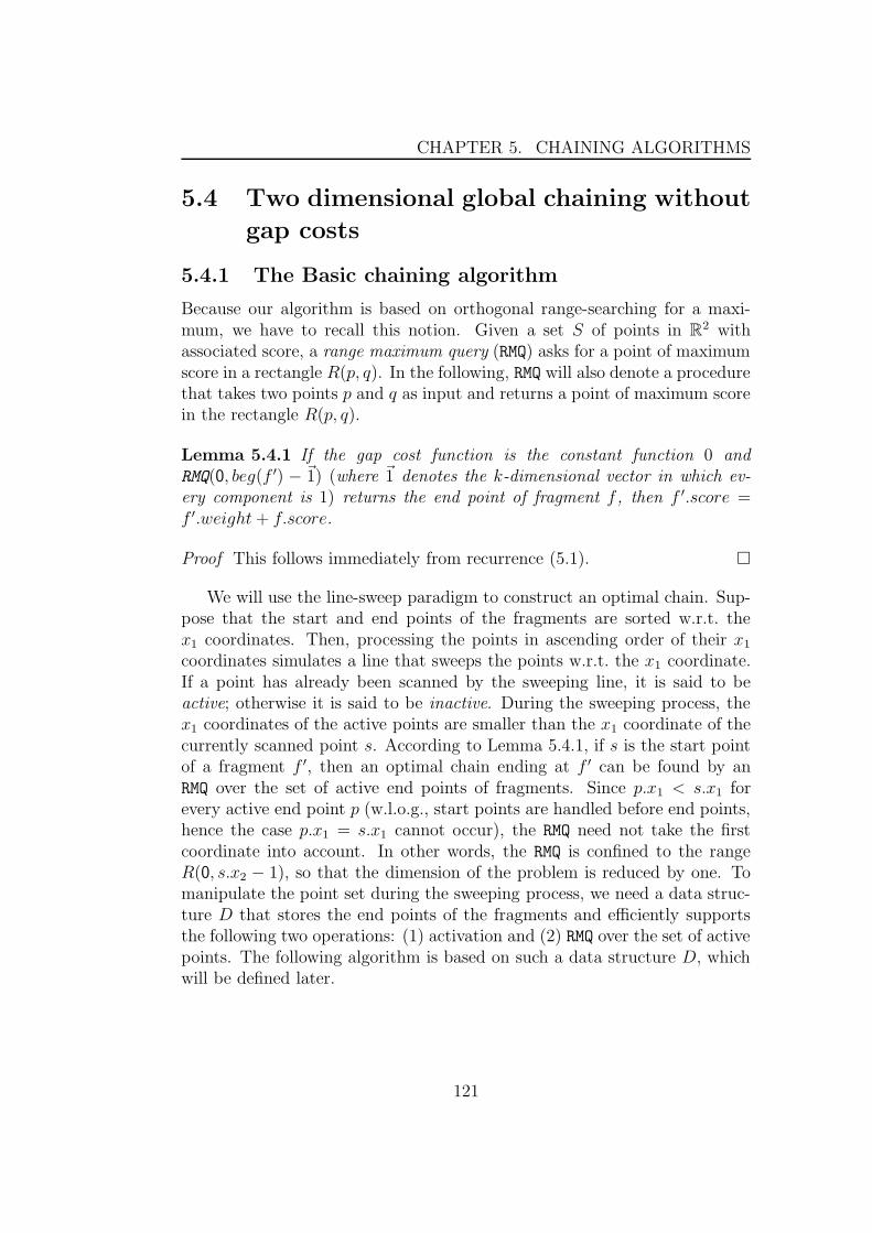
CHAPTER 5. CHAINING ALGORITHMS
5.4 Two dimensional global chaining without
gap costs
5.4.1 The Basic chaining algorithm
Because our algorithm is based on orthogonal range-searching for a maxi-mum, we have to recall this notion. Given a set S of points in R
2 withassociated score, a range maximum query (RMQ) asks for a point of maximumscore in a rectangle R(p, q). In the following, RMQ will also denote a procedurethat takes two points p and q as input and returns a point of maximum scorein the rectangle R(p, q).
Lemma 5.4.1 If the gap cost function is the constant function 0 andRMQ(0, beg(f ′) − ~1) (where ~1 denotes the k-dimensional vector in which ev-ery component is 1) returns the end point of fragment f , then f ′.score =f ′.weight + f.score.
Proof This follows immediately from recurrence (5.1). �
We will use the line-sweep paradigm to construct an optimal chain. Sup-pose that the start and end points of the fragments are sorted w.r.t. thex1 coordinates. Then, processing the points in ascending order of their x1
coordinates simulates a line that sweeps the points w.r.t. the x1 coordinate.If a point has already been scanned by the sweeping line, it is said to beactive; otherwise it is said to be inactive. During the sweeping process, thex1 coordinates of the active points are smaller than the x1 coordinate of thecurrently scanned point s. According to Lemma 5.4.1, if s is the start pointof a fragment f ′, then an optimal chain ending at f ′ can be found by anRMQ over the set of active end points of fragments. Since p.x1 < s.x1 forevery active end point p (w.l.o.g., start points are handled before end points,hence the case p.x1 = s.x1 cannot occur), the RMQ need not take the firstcoordinate into account. In other words, the RMQ is confined to the rangeR(0, s.x2 − 1), so that the dimension of the problem is reduced by one. Tomanipulate the point set during the sweeping process, we need a data struc-ture D that stores the end points of the fragments and efficiently supportsthe following two operations: (1) activation and (2) RMQ over the set of activepoints. The following algorithm is based on such a data structure D, whichwill be defined later.
121

CHAPTER 5. CHAINING ALGORITHMS
Algorithm 5.4.2 2-dimensional chaining of m fragments
Sort all start and end points of the m fragments in ascending order w.r.t.their x1 coordinate and store them in the array points; because we includethe end point of the origin and the start point of the terminus, there are2m + 2 points.Store all end points of the fragments (ignoring their x1 coordinate) asinactive (in the 1-dimensional) data structure D.for i := 1 to 2m + 2
if points[i] is the start point of fragment f ′ thenq := RMQ(0, points[i].x2 − 1)determine the fragment f with end(f) = qf ′.prec := ff ′.score := f ′.weight + f.score
else /? points[i] is end point of a fragment f ′ ?/activate points[i].x2 in D /? activate with score f ′.score ?/
In the algorithm, f ′.prec denotes the preceding fragment of f ′ in a chain. Itis an immediate consequence of Lemma 5.4.1 that Algorithm 5.4.2 finds anoptimal chain. One can output this chain by tracing back the prec pointersfrom the terminus to the origin. The complexity of the algorithm dependsof course on how the data structure D is implemented. In the following, wewill address three alternatives of the data structure D.
5.4.2 Answering RMQ with activation
Alternative 1: Priority search tree
To answer RMQ with activation, we can use the priority search tree devisedby McCreight [102]. Let S be a set of m one dimensional points. For ease ofpresentation, assume that no two points have the same coordinate (In [102],it is shown how to proceed if this is not the case). The priority search treeof S is a minimum-height binary search tree T with m leaves, whose ithleftmost leaf stores the point in S with the ith smallest coordinate. Let v.Land v.R denote the left and right child, respectively, of an interior node v. Toeach interior node v of T , we associate a canonical subset Cv ⊆ S containingthe points stored at the leaves of the subtree rooted at v. Furthermore, vstores the values lv, hv, and pv, where lv denotes the smallest coordinate ofany point in Cv, hv denotes the largest coordinate of any point in Cv and pv
denotes the point of highest score (priority) in Cv that has not been storedat a shallower depth in T . If such a point does not exist, pv is undefined;see Figure 5.2. We will call hv.L the splitting coordinate of node v because it
122
CHAPTER 5. CHAINING ALGORITHMS
������������
���������
���������
����������������
����������������
- - -- -
RMQ(0,19)87
P12
31292725241
27
P12 P16
29
P14P13
3
2925
P15
- -
P1
P1
15
8
1412974
P4
P10
3
P9
P7
P5
P2
P9
17
P10
P11
20
P9
P4
P11
P7
8 8
P8
8 8
P8
2220
20
17 224
15
12
9 141
247
P3 P5
8
P10
8 30 21 9 8425 79 56
P11
P6
coordinate
score
Figure 5.2: Priority search tree: The points with score −∞ are inactive; the othersare active. The value hv.L in every interior node v is the coordinate that separatesthe points in its left subtree v.L from those occurring in its right subtree v.R.The pv value of v is depicted as a “child” between v.L and v.R. If it is missing,then pv is undefined. The colored nodes are visited in answering the RMQ(0, 19).The hatched boxes contain the modified pv values when point p12 is activated withscore 87.
is the coordinate that separates the points in its left subtree v.L from thoseoccurring in its right subtree v.R. In essence, the priority search tree of S isa variant of a balanced binary search tree and a heap (i.e., priority queue).It can be built in O(m log m) time and O(m) space.
In Algorithm 5.4.2, storing all end points of the fragments as inactive isachieved by constructing the priority search tree of the end points, whereeach point stored at a leaf has score −∞ and pv is undefined for each interiornode v.
In a priority search tree T , a point q can be activated with priority scorein O(logm) time as follows. First, update the value of q.score by q.score :=score. Second, update the pv values by a traversal of T that starts at theroot. Suppose node v is visited in the traversal. If v is a leaf, there is nothingto do. If v is an interior node with pv.score ≤ q.score, then swap q and pv
(more precisely, exchange the values of the variables q and pv); otherwiseretain q and pv unchanged. Then determine where the procedure is to becontinued. If q ≤ hv.L, proceed recursively with the left child v.L of v.Otherwise, proceed recursively with the right child v.R of v.
A range maximum query RMQ(0, q) can be answered in O(log m) time asfollows. We traverse the priority search tree starting at the root. During thetraversal, we maintain a variable max point that stores the point of highestscore in the range R(0, q) seen so far (initially, max point is undefined).
123

CHAPTER 5. CHAINING ALGORITHMS
Suppose node v is visited in the traversal. If v is a leaf storing the pointpv, then we proceed as in case (1) below. If v is an interior node, then wedistinguish the cases (1) pv ≤ q and (2) pv > q. In case (1), if pv.score ≥max point.score, then we update max point by max point := pv. In case(2), if q ≤ hv.L, then we recursively proceed with the left child v.L of v;otherwise, we recursively proceed with both children of v. Describing thisprocedure on a higher level, we identify during the traversal a set of nodeswhich we call canonical nodes (w.r.t. the given range query). The set ofthese canonical nodes is the smallest set of nodes v1, . . . , v` of the tree suchthat ]`
j=1Cvj= RQ(0, q). (] denotes disjoint union.). By examining the
priority information of the canonical nodes, the node of highest score can beidentified.
Another example of a data structure that supports RMQ with activation isthe kd-tree [24]. In essence, the one-dimensional kd-tree coincides with thepriority search tree, but the operations on kd-trees are accelerated in practiceby a collection of programming tricks; see [24].
Alternative 2: Dynamic priority search tree
The priority search tree described above is a semi-dynamic data structure,in the sense that it is constructed for all the points at once and the pointsare neither inserted nor deleted, rather activated and deactivated in the datastructure. For our applications, the usage of such semi-dynamic data struc-tures is satisfactory, because all the fragments are pre-generated in the firstphase of the anchor based strategy. Nevertheless, the usage of dynamic datastructures for answering RMQs should be addressed. If a dynamic data struc-ture is employed, then the points are inserted when they are scanned anddeleted when they are no longer needed. The priority search tree can bedynamized so that the points are inserted when they are scanned as follows.The fixed tree structure is replaced with red-black tree structure. The tree isinitially empty. When a point is scanned, it is inserted in the tree, the treeis re-balanced, and the spatial information, i.e., h.v, is updated. After theinsertion, the score of the point is updated in the tree as done before for thesemi-dynamic tree. The insertion of a point, including the re-balancing andthe updating of the spatial information, takes O(log m) time [122]. Updatingthe score takes also O(log m) time. Hence, the time complexity of an RMQ
with activation using a dynamic priority search tree is still O(log m).The advantage of using a dynamic version is that online chaining (i.e.,
fragments are chained while being generated) becomes possible. That is, ifthe fragments are generated such that their order w.r.t. one of the sequencesis maintained, then the newly generated fragments are the currently scanned
124
CHAPTER 5. CHAINING ALGORITHMS
points and they can be chained to the previously scanned (generated) ones.However, there is no improvement, even in practice, in the space consumptionof the algorithm. This is because no deletion operations take place, whichresults in that all the the points are eventually inserted in the tree. Theworst case running time does also not improve, because it is still bounded bythe number of elements that can be inserted in D. This number is O(m).
Alternative 3: Priority queue
Because the RMQ is in the range R(0, q), i.e., the origin 0 is always the lower-left corner, and because there is no deactivation operation, we can furtherreduce the complexity of answering RMQ with activation. What is required isjust a one dimensional dynamic data structure D that supports the followingoperations:1
• insert(q): if q is not in D, then put q into D; otherwise update itssatellite information, i.e., the fragment corresponding to q
• delete(q): remove q from D.
• predecessor(q): give the largest element ≤ q in D.
• successor(q): give the smallest element > q in D.
If every end point q is activated as shown in Algorithm 5.4.3, then answer-ing RMQ(0, q) boils down to computing predecessor(q) in D. It is importantto note that the operations predecessor(q) and successor(q) are always well-defined if we initialize the data structure D with the origin and the terminuspoints.
Algorithm 5.4.3 Implementation of the operation activate in the data struc-ture D
if (q.score > predecessor(q).score) theninsert(q)while (q.score > successor(q).score)
delete(successor(q))
Note that the following invariant is maintained: If 0 ≤ q1 < q2 < · · · <q` ≤ n are the entries in the data structure D, then q1.score ≤ q2.score ≤· · · ≤ q`.score.
1In the dynamic case, the sentence preceding the for loop in Algorithm 5.4.2 must bedeleted.
125
CHAPTER 5. CHAINING ALGORITHMS
Many data structures that support the aforementioned operations arealready known. For example, the priority queues devised by van Emde Boas[132, 133] and Johnson’s improvement [74] support the operations in timeO(log log N) and space O(N), provided that every q satisfies 1 ≤ q ≤ N .The space requirement can be reduced to O(n), where n denotes the numberof elements stored in the priority queue; see [103]. Recall that a fragmentcorresponds to segments of the strings S1 and S2 that are similar. W.l.o.g., wemay assume that n1 = |S1| ≤ |S2| = n2 (otherwise, we swap the sequences).In Algorithm 5.4.2, sorting all start and end points of the m fragments inascending order w.r.t. their x1 coordinate by counting sort (see, e.g., [40])takes O(n1) time. Since Algorithm 5.4.2 employs at most O(m) priorityqueue operations, each of which takes time O(log log n2), the overall timecomplexity of this implementation is O(n1 + m log log n2). However, in mostapplications m is relatively small compared to n2, so that it is advantageousto sort the start and end points of the m fragments in O(m logm) time. Ifthe fragments are generated such that they are already ordered w.r.t. onesequence, say S1, the worst case time complexity reduces to O(m log log n2).
RMQ based on the operations insert, delete, predecessor, and successorhas the advantage of reducing, in practice, the space requirement of thechaining algorithm. Clearly, the reason for this is that only the points thatare candidate to be part of an optimal chain are stored in the main memorywhile those that are not are deleted. Unfortunately, this approach cannotbe extended to higher dimensions and it is not possible to include othervariations such as gap constraints; this point will be explained in detail inSection 5.8.
5.5 Higher dimensional chaining without gap
costs
As mentioned in Section 5.3, the graph based approach also solves the chain-ing problem for more than two genomes. However, the running time of thischaining algorithm is quadratic in the number of fragments. This can be aserious drawback if the number of fragments is large. A big advantage of ourAlgorithm 5.4.2 is that it can be readily extended to higher dimensions. Inorder to chain k-dimensional fragments, the 1-dimensional data structure Din Algorithm 5.4.2 has to be replaced with a (k − 1)-dimensional data struc-ture that supports range maximum queries and activation. In the following,we will outline two such data structures for dimension d = k− 1, namely therange tree and the kd -tree.
126
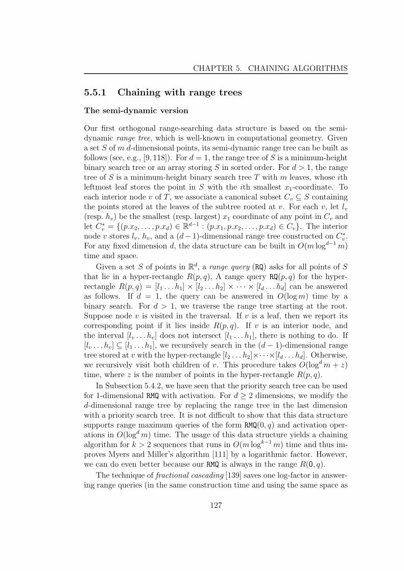
CHAPTER 5. CHAINING ALGORITHMS
5.5.1 Chaining with range trees
The semi-dynamic version
Our first orthogonal range-searching data structure is based on the semi-dynamic range tree, which is well-known in computational geometry. Givena set S of m d-dimensional points, its semi-dynamic range tree can be built asfollows (see, e.g., [9, 118]). For d = 1, the range tree of S is a minimum-heightbinary search tree or an array storing S in sorted order. For d > 1, the rangetree of S is a minimum-height binary search tree T with m leaves, whose ithleftmost leaf stores the point in S with the ith smallest x1-coordinate. Toeach interior node v of T , we associate a canonical subset Cv ⊆ S containingthe points stored at the leaves of the subtree rooted at v. For each v, let lv(resp. hv) be the smallest (resp. largest) x1 coordinate of any point in Cv andlet C∗
v = {(p.x2, . . . , p.xd) ∈ Rd−1 : (p.x1, p.x2, . . . , p.xd) ∈ Cv}. The interior
node v stores lv, hv, and a (d− 1)-dimensional range tree constructed on C∗v .
For any fixed dimension d, the data structure can be built in O(m logd−1 m)time and space.
Given a set S of points in Rd, a range query (RQ) asks for all points of S
that lie in a hyper-rectangle R(p, q), A range query RQ(p, q) for the hyper-rectangle R(p, q) = [l1 . . . h1] × [l2 . . . h2] × · · · × [ld . . . hd] can be answeredas follows. If d = 1, the query can be answered in O(log m) time by abinary search. For d > 1, we traverse the range tree starting at the root.Suppose node v is visited in the traversal. If v is a leaf, then we report itscorresponding point if it lies inside R(p, q). If v is an interior node, andthe interval [lv . . . hv] does not intersect [l1 . . . h1], there is nothing to do. If[lv . . . hv] ⊆ [l1 . . . h1], we recursively search in the (d − 1)-dimensional rangetree stored at v with the hyper-rectangle [l2 . . . h2]×· · ·×[ld . . . hd]. Otherwise,we recursively visit both children of v. This procedure takes O(logd m + z)time, where z is the number of points in the hyper-rectangle R(p, q).
In Subsection 5.4.2, we have seen that the priority search tree can be usedfor 1-dimensional RMQ with activation. For d ≥ 2 dimensions, we modify thed-dimensional range tree by replacing the range tree in the last dimensionwith a priority search tree. It is not difficult to show that this data structuresupports range maximum queries of the form RMQ(0, q) and activation oper-ations in O(logd m) time. The usage of this data structure yields a chainingalgorithm for k > 2 sequences that runs in O(m logk−1 m) time and thus im-proves Myers and Miller’s algorithm [111] by a logarithmic factor. However,we can do even better because our RMQ is always in the range R(0, q).
The technique of fractional cascading [139] saves one log-factor in answer-ing range queries (in the same construction time and using the same space as
127

CHAPTER 5. CHAINING ALGORITHMS
p6
p2
p4
p5
p3p1
p8
p7
(3, 29)(9, 33)
(21, 15)(13, 19)
(7, 1)
(17, 27)
query rectangle [0 .. 22]x[0 .. 28]
(31, 23)
(25, 5)
Figure 5.3: A set of points and a query rectangle for the example of Figure 5.4.
the original range tree). Here we focus on range queries of the form RQ(0, q)because we want to modify it to answer range maximum queries of the formRMQ(0, q) efficiently. For ease of presentation, we consider the case d = 2.In this case, the range tree is a binary search tree (called x-tree) of arrays(called y-arrays). Let v be a node in the x-tree and let v.L and v.R be itsleft and right children. The y-array Av of v contains all the points in Cv
sorted in ascending order w.r.t. their y coordinate. Every element p ∈ Av
has two downstream pointers: The left pointer Lptr and the right pointerRptr. The left pointer Lptr points to the largest (i.e., rightmost) element q1
in Av.L such that q1 ≤ p (Lptr is a NULL pointer if such an element doesnot exist). In an implementation, Lptr is the index with Av.L[Lptr] = q1.Analogously, the right pointer Rptr points to the largest element q2 of Av.R
such that q2 ≤ p. Figure 5.4 shows an example of this structure.Locating all the points in a rectangle R(0, (h1, h2)) is done in two stages.
In the first stage, a binary search is performed over the y-array of theroot node of the x-tree to locate the rightmost point ph2 such that ph2.y ∈[0 . . . h2]. Then, in the second stage, the x-tree is traversed (while keep-ing track of the downstream pointers) to locate the rightmost leaf ph1 suchthat ph1.x ∈ [0 . . . h1]. During the traversal of the x-tree, we identify aset of nodes which we call canonical nodes (w.r.t. the given range query).The set of canonical nodes is the smallest set of nodes v1, . . . , v` of x-treesuch that ]`
j=1Cvj= RQ(0, (h1,∞)). (] denotes disjoint union.) In other
words, P := ]`j=1Avj
= ]`j=1Cvj
contains every point p ∈ S such thatp.x ∈ [0 . . . h1]. However, not every point p ∈ P satisfies p.y ∈ [0 . . . h2].Here, the downstream pointers come into play. As already mentioned, thedownstream pointers are followed while traversing the x-tree, and to fol-low one pointer takes constant time. If we encounter a canonical node vj,then the element ej, to which the last downstream pointer points, partitions
128
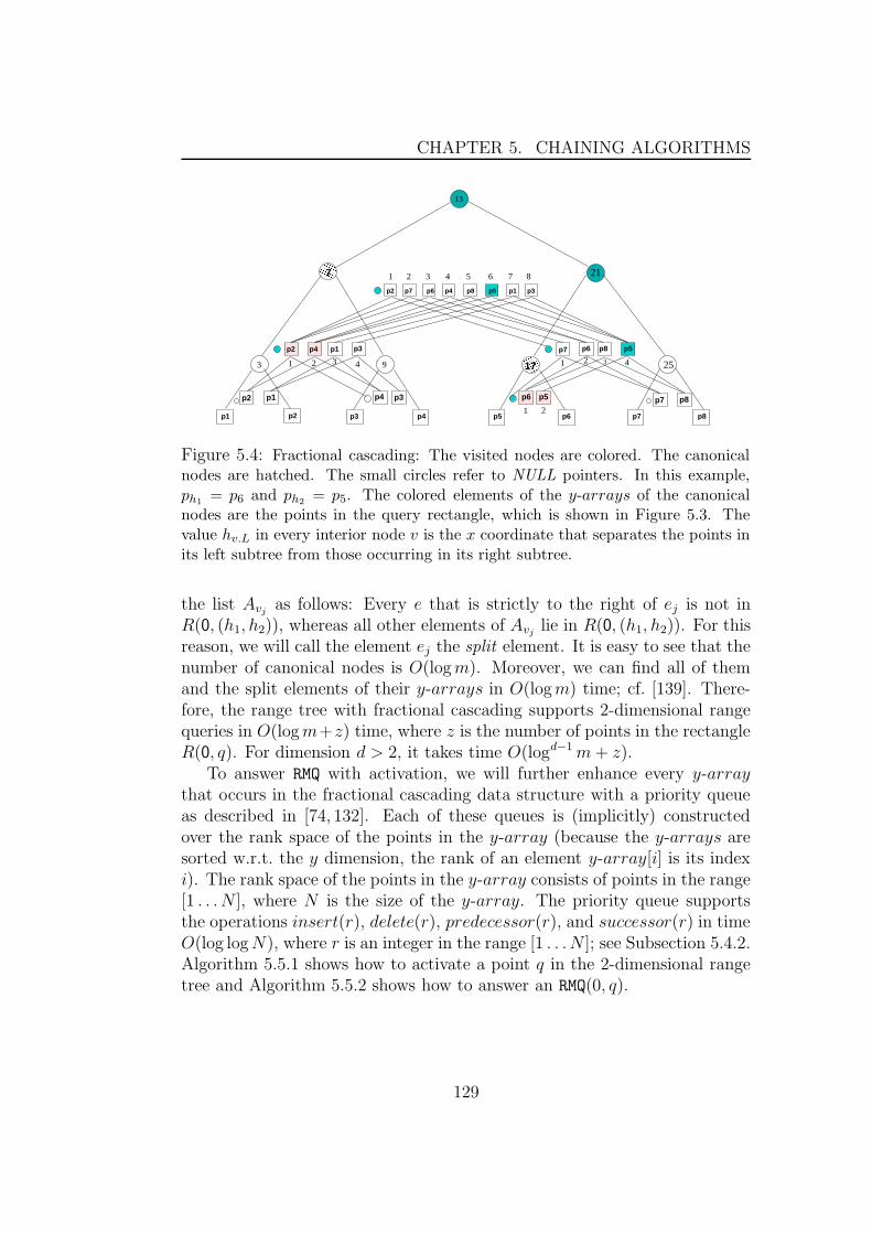
CHAPTER 5. CHAINING ALGORITHMS
p1 p2 p8p4 p5 p6p3
p7 p8p2 p1
p3p1p2 p7
p7
���������������
���������������
p6 p5
���������
���������
p3
p8p6p7p3p1
p8p4
p4
p5p2
p5p6
p4
21
25
7
1793
1 2 3 4 5 6 7 8
3 2 31 4 1 4
1 2
2
13
Figure 5.4: Fractional cascading: The visited nodes are colored. The canonicalnodes are hatched. The small circles refer to NULL pointers. In this example,ph1 = p6 and ph2 = p5. The colored elements of the y-arrays of the canonicalnodes are the points in the query rectangle, which is shown in Figure 5.3. Thevalue hv.L in every interior node v is the x coordinate that separates the points inits left subtree from those occurring in its right subtree.
the list Avjas follows: Every e that is strictly to the right of ej is not in
R(0, (h1, h2)), whereas all other elements of Avjlie in R(0, (h1, h2)). For this
reason, we will call the element ej the split element. It is easy to see that thenumber of canonical nodes is O(log m). Moreover, we can find all of themand the split elements of their y-arrays in O(logm) time; cf. [139]. There-fore, the range tree with fractional cascading supports 2-dimensional rangequeries in O(log m+z) time, where z is the number of points in the rectangleR(0, q). For dimension d > 2, it takes time O(logd−1 m + z).
To answer RMQ with activation, we will further enhance every y-arraythat occurs in the fractional cascading data structure with a priority queueas described in [74, 132]. Each of these queues is (implicitly) constructedover the rank space of the points in the y-array (because the y-arrays aresorted w.r.t. the y dimension, the rank of an element y-array[i] is its indexi). The rank space of the points in the y-array consists of points in the range[1 . . . N ], where N is the size of the y-array. The priority queue supportsthe operations insert(r), delete(r), predecessor(r), and successor(r) in timeO(log log N), where r is an integer in the range [1 . . . N ]; see Subsection 5.4.2.Algorithm 5.5.1 shows how to activate a point q in the 2-dimensional rangetree and Algorithm 5.5.2 shows how to answer an RMQ(0, q).
129
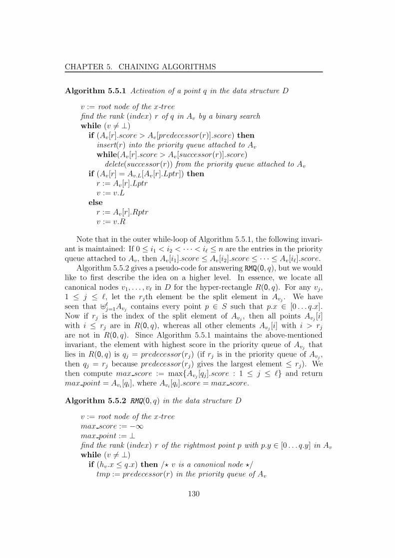
CHAPTER 5. CHAINING ALGORITHMS
Algorithm 5.5.1 Activation of a point q in the data structure D
v := root node of the x-treefind the rank (index) r of q in Av by a binary searchwhile (v 6= ⊥)
if (Av[r].score > Av[predecessor(r)].score) theninsert(r) into the priority queue attached to Av
while(Av[r].score > Av[successor(r)].score)delete(successor(r)) from the priority queue attached to Av
if (Av[r] = Av.L[Av[r].Lptr]) thenr := Av[r].Lptrv := v.L
elser := Av[r].Rptrv := v.R
Note that in the outer while-loop of Algorithm 5.5.1, the following invari-ant is maintained: If 0 ≤ i1 < i2 < · · · < i` ≤ n are the entries in the priorityqueue attached to Av, then Av[i1].score ≤ Av[i2].score ≤ · · · ≤ Av[i`].score.
Algorithm 5.5.2 gives a pseudo-code for answering RMQ(0, q), but we wouldlike to first describe the idea on a higher level. In essence, we locate allcanonical nodes v1, . . . , v` in D for the hyper-rectangle R(0, q). For any vj,1 ≤ j ≤ `, let the rjth element be the split element in Avj
. We haveseen that ]`
j=1Avjcontains every point p ∈ S such that p.x ∈ [0 . . . q.x].
Now if rj is the index of the split element of Avj, then all points Avj
[i]with i ≤ rj are in R(0, q), whereas all other elements Avj
[i] with i > rj
are not in R(0, q). Since Algorithm 5.5.1 maintains the above-mentionedinvariant, the element with highest score in the priority queue of Avj
thatlies in R(0, q) is qj = predecessor(rj) (if rj is in the priority queue of Avj
,then qj = rj because predecessor(rj) gives the largest element ≤ rj). Wethen compute max score := max{Avj
[qj].score : 1 ≤ j ≤ `} and returnmax point = Avi
[qi], where Avi[qi].score = max score.
Algorithm 5.5.2 RMQ(0, q) in the data structure D
v := root node of the x-treemax score := −∞max point := ⊥find the rank (index) r of the rightmost point p with p.y ∈ [0 . . . q.y] in Av
while (v 6= ⊥)if (hv.x ≤ q.x) then /? v is a canonical node ?/
tmp := predecessor(r) in the priority queue of Av
130
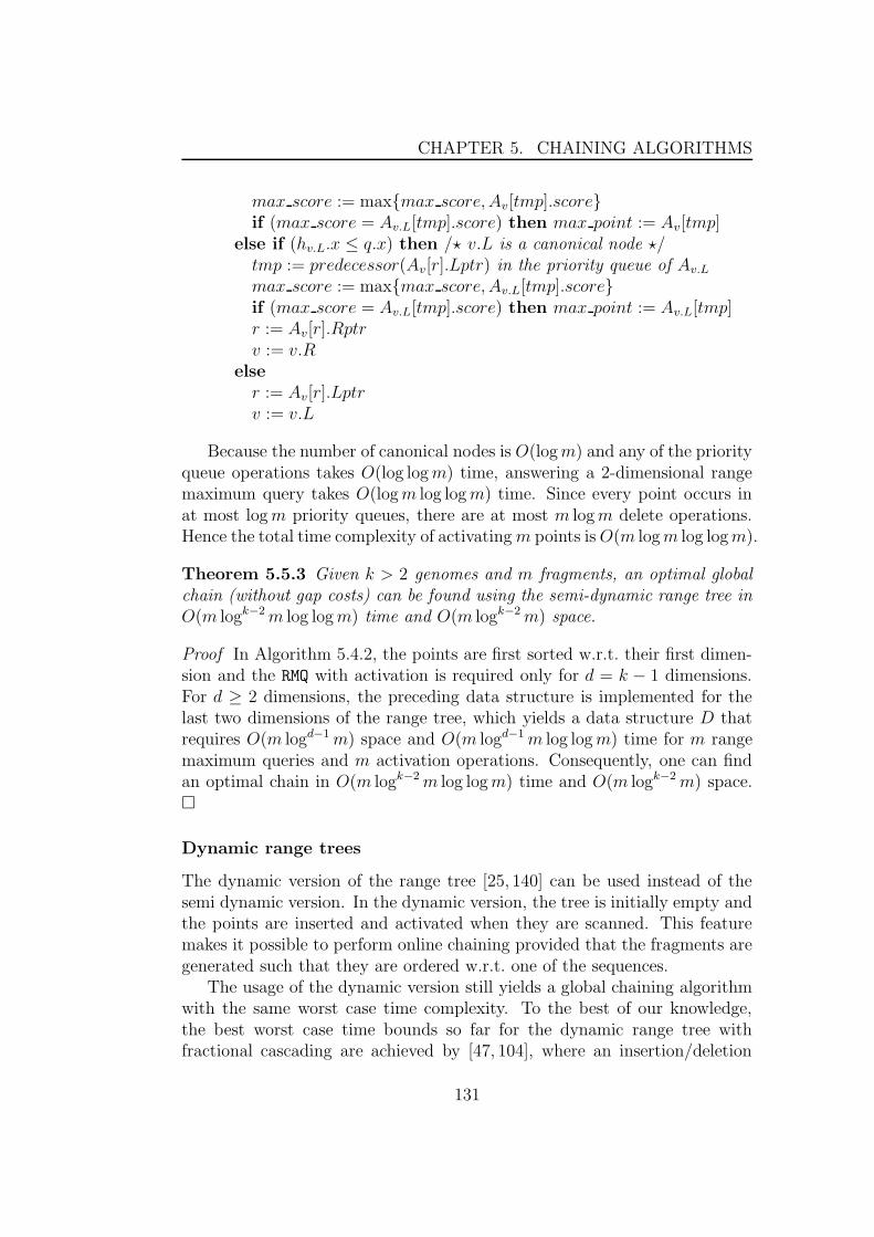
CHAPTER 5. CHAINING ALGORITHMS
max score := max{max score, Av[tmp].score}if (max score = Av.L[tmp].score) then max point := Av[tmp]
else if (hv.L.x ≤ q.x) then /? v.L is a canonical node ?/tmp := predecessor(Av[r].Lptr) in the priority queue of Av.L
max score := max{max score, Av.L[tmp].score}if (max score = Av.L[tmp].score) then max point := Av.L[tmp]r := Av[r].Rptrv := v.R
elser := Av[r].Lptrv := v.L
Because the number of canonical nodes is O(log m) and any of the priorityqueue operations takes O(log log m) time, answering a 2-dimensional rangemaximum query takes O(log m log log m) time. Since every point occurs inat most log m priority queues, there are at most m log m delete operations.Hence the total time complexity of activating m points is O(m log m log log m).
Theorem 5.5.3 Given k > 2 genomes and m fragments, an optimal globalchain (without gap costs) can be found using the semi-dynamic range tree inO(m logk−2 m log log m) time and O(m logk−2 m) space.
Proof In Algorithm 5.4.2, the points are first sorted w.r.t. their first dimen-sion and the RMQ with activation is required only for d = k − 1 dimensions.For d ≥ 2 dimensions, the preceding data structure is implemented for thelast two dimensions of the range tree, which yields a data structure D thatrequires O(m logd−1 m) space and O(m logd−1 m log log m) time for m rangemaximum queries and m activation operations. Consequently, one can findan optimal chain in O(m logk−2 m log log m) time and O(m logk−2 m) space.�
Dynamic range trees
The dynamic version of the range tree [25, 140] can be used instead of thesemi dynamic version. In the dynamic version, the tree is initially empty andthe points are inserted and activated when they are scanned. This featuremakes it possible to perform online chaining provided that the fragments aregenerated such that they are ordered w.r.t. one of the sequences.
The usage of the dynamic version still yields a global chaining algorithmwith the same worst case time complexity. To the best of our knowledge,the best worst case time bounds so far for the dynamic range tree withfractional cascading are achieved by [47, 104], where an insertion/deletion
131
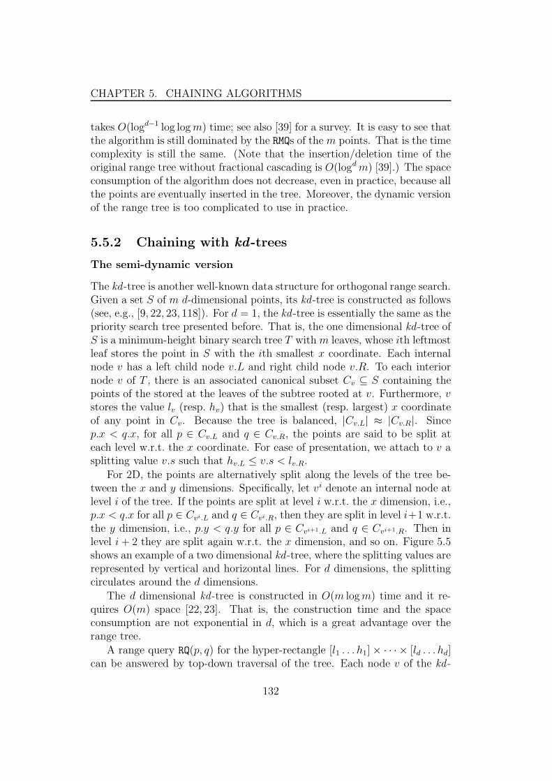
CHAPTER 5. CHAINING ALGORITHMS
takes O(logd−1 log log m) time; see also [39] for a survey. It is easy to see thatthe algorithm is still dominated by the RMQs of the m points. That is the timecomplexity is still the same. (Note that the insertion/deletion time of theoriginal range tree without fractional cascading is O(logd m) [39].) The spaceconsumption of the algorithm does not decrease, even in practice, because allthe points are eventually inserted in the tree. Moreover, the dynamic versionof the range tree is too complicated to use in practice.
5.5.2 Chaining with kd-trees
The semi-dynamic version
The kd -tree is another well-known data structure for orthogonal range search.Given a set S of m d-dimensional points, its kd -tree is constructed as follows(see, e.g., [9, 22, 23, 118]). For d = 1, the kd -tree is essentially the same as thepriority search tree presented before. That is, the one dimensional kd -tree ofS is a minimum-height binary search tree T with m leaves, whose ith leftmostleaf stores the point in S with the ith smallest x coordinate. Each internalnode v has a left child node v.L and right child node v.R. To each interiornode v of T , there is an associated canonical subset Cv ⊆ S containing thepoints of the stored at the leaves of the subtree rooted at v. Furthermore, vstores the value lv (resp. hv) that is the smallest (resp. largest) x coordinateof any point in Cv. Because the tree is balanced, |Cv.L| ≈ |Cv.R|. Sincep.x < q.x, for all p ∈ Cv.L and q ∈ Cv.R, the points are said to be split ateach level w.r.t. the x coordinate. For ease of presentation, we attach to v asplitting value v.s such that hv.L ≤ v.s < lv.R.
For 2D, the points are alternatively split along the levels of the tree be-tween the x and y dimensions. Specifically, let vi denote an internal node atlevel i of the tree. If the points are split at level i w.r.t. the x dimension, i.e.,p.x < q.x for all p ∈ Cvi.L and q ∈ Cvi.R, then they are split in level i+1 w.r.t.the y dimension, i.e., p.y < q.y for all p ∈ Cvi+1.L and q ∈ Cvi+1.R. Then inlevel i + 2 they are split again w.r.t. the x dimension, and so on. Figure 5.5shows an example of a two dimensional kd -tree, where the splitting values arerepresented by vertical and horizontal lines. For d dimensions, the splittingcirculates around the d dimensions.
The d dimensional kd -tree is constructed in O(m log m) time and it re-quires O(m) space [22, 23]. That is, the construction time and the spaceconsumption are not exponential in d, which is a great advantage over therange tree.
A range query RQ(p, q) for the hyper-rectangle [l1 . . . h1] × · · · × [ld . . . hd]can be answered by top-down traversal of the tree. Each node v of the kd -
132
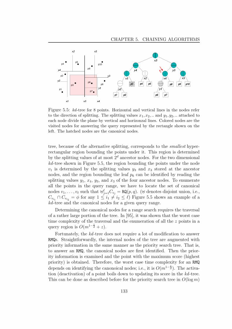
CHAPTER 5. CHAINING ALGORITHMS
�����������������������������������
�������������������������
��������������������
������������
p1 p2
p4 p5 p8 p9
x1 x2
x3
x4 x5
y4 y3
y2 y1
p3
x3 x4
x2 x5
y1
y2
y3
y4
x1
v1
p1
p2
p3
p9
p10
p6
p4p5
p8
p7
p7
p10
p6
Figure 5.5: kd -tree for 8 points. Horizontal and vertical lines in the nodes referto the direction of splitting. The splitting values x1, x2, .. and y1, y2, .. attached toeach node divide the plane by vertical and horizonzal lines. Colored nodes are thevisited nodes for answering the query represented by the rectangle shown on theleft. The hatched nodes are the canonical nodes.
tree, because of the alternative splitting, corresponds to the smallest hyper-rectangular region bounding the points under it. This region is determinedby the splitting values of at most 2d ancestor nodes. For the two dimensionalkd -tree shown in Figure 5.5, the region bounding the points under the nodev1 is determined by the splitting values y3 and x3 stored at the ancestornodes, and the region bounding the leaf p6 can be identified by reading thesplitting values y1, x4, y3, and x3 of the four ancestor nodes. To enumerateall the points in the query range, we have to locate the set of canonicalnodes v1, . . . , v` such that ]`
j=1Cvj= RQ(p, q). (] denotes disjoint union, i.e.,
Cvi1∩ Cvi2
= φ for any 1 ≤ i1 6= i2 ≤ `) Figure 5.5 shows an example of akd -tree and the canonical nodes for a given query range.
Determining the canonical nodes for a range search requires the traversalof a rather large portion of the tree. In [95], it was shown that the worst casetime complexity of the traversal and the enumeration of all the z points in aquery region is O(m1− 1
d + z).
Fortunately, the kd -tree does not require a lot of modification to answerRMQs. Straightforwardly, the internal nodes of the tree are augmented withpriority information in the same manner as the priority search tree. That is,to answer an RMQ, the canonical nodes are first identified. Then the prior-ity information is examined and the point with the maximum score (highestpriority) is obtained. Therefore, the worst case time complexity for an RMQ
depends on identifying the canonoical nodes; i.e., it is O(m1− 1d ). The activa-
tion (deactivation) of a point boils down to updating its score in the kd -tree.This can be done as described before for the priority search tree in O(log m)
133

CHAPTER 5. CHAINING ALGORITHMS
time; see [24] for more details. Interestingly, Bently [24] has shown thatthe running time of the semi-dynamic kd -tree operations, such as answeringRMQs, activation and deactivation, can be improved in practice using a set ofprogramming tricks.
Theorem 5.5.4 Given k > 2 genomes and m fragments, an optimal globalchain (without gap costs) can be found using a semi-dynamic kd-tree in
O((k − 1) m2− 1k−1 ) time and O(m) space.
Proof In Algorithm 5.4.2, the points are first sorted w.r.t. their first dimen-sion and the RMQ with activation is required only for d = k − 1 dimensions.For d dimensions, the kd -tree is constructed in O(m log m) time and it re-
quires O(m) space. Answering an RMQ takes O(dm1− 1d ) time and O(m) space.
Consequently, one can find an optimal chain, using the line sweep paradigm,
in O((k − 1) m2− 1k−1 ) time and O(m) space. �
Dynamic kd-trees
As mentioned before, a dynamic kd -tree can be used for the global chaining.However, using a dynamic version will not improve the worst case runningtime of the algorithm. Worse, the time complexity of the RMQ is higherwith a certain factor that depends on the dynamization technique involved[41, 55, 87, 129]; see also [39] for a survey. To the best of our knoweldge, the
best query time is achieved by [87], where the factor is O(log1d m). (The
insertion of m points still takes O(m logm) time.) The space consumptionwill not decrease, even in practice, because all the points are eventuallyinserted in the tree. Moreover, the dynamic versions are more complicatedthan the semi-dynamic one.
Range trees versus kd-trees
Theoretically, there is a tradeoff between the kd -tree and the range tree. Onthe one hand, the worst case query time of the range tree is better thanthat of the kd -tree. On the other hand, the construction time and spaceconsumption of the kd -tree is much less than that of the range tree. In therange tree, both the construction time and the space consumption increaseexponentially with d, while in the kd -tree the space consumption is linearand the construction time is O(m log m), i.e., not exponential in d.
We have implemented the two data structures and measured the construc-tion and query time. The results, which are summarized in Table 5.1, showthat the kd -tree is superior to the range tree in practice. This is particularly
134
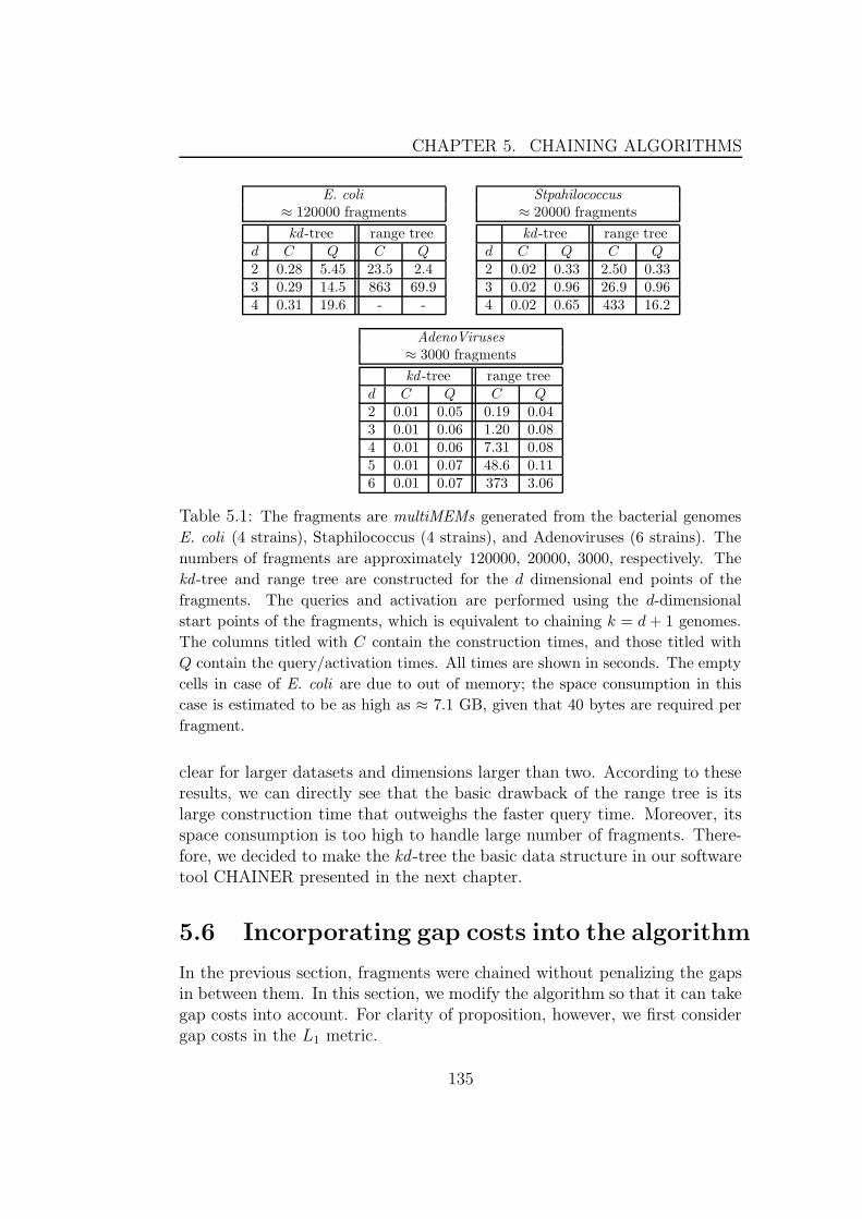
CHAPTER 5. CHAINING ALGORITHMS
E. coli
≈ 120000 fragments
kd -tree range treed C Q C Q
2 0.28 5.45 23.5 2.43 0.29 14.5 863 69.94 0.31 19.6 - -
Stpahilococcus
≈ 20000 fragments
kd -tree range treed C Q C Q
2 0.02 0.33 2.50 0.333 0.02 0.96 26.9 0.964 0.02 0.65 433 16.2
AdenoViruses
≈ 3000 fragments
kd -tree range treed C Q C Q
2 0.01 0.05 0.19 0.043 0.01 0.06 1.20 0.084 0.01 0.06 7.31 0.085 0.01 0.07 48.6 0.116 0.01 0.07 373 3.06
Table 5.1: The fragments are multiMEMs generated from the bacterial genomes
E. coli (4 strains), Staphilococcus (4 strains), and Adenoviruses (6 strains). The
numbers of fragments are approximately 120000, 20000, 3000, respectively. The
kd -tree and range tree are constructed for the d dimensional end points of the
fragments. The queries and activation are performed using the d-dimensional
start points of the fragments, which is equivalent to chaining k = d + 1 genomes.
The columns titled with C contain the construction times, and those titled with
Q contain the query/activation times. All times are shown in seconds. The empty
cells in case of E. coli are due to out of memory; the space consumption in this
case is estimated to be as high as ≈ 7.1 GB, given that 40 bytes are required per
fragment.
clear for larger datasets and dimensions larger than two. According to theseresults, we can directly see that the basic drawback of the range tree is itslarge construction time that outweighs the faster query time. Moreover, itsspace consumption is too high to handle large number of fragments. There-fore, we decided to make the kd -tree the basic data structure in our softwaretool CHAINER presented in the next chapter.
5.6 Incorporating gap costs into the algorithm
In the previous section, fragments were chained without penalizing the gapsin between them. In this section, we modify the algorithm so that it can takegap costs into account. For clarity of proposition, however, we first considergap costs in the L1 metric.
135
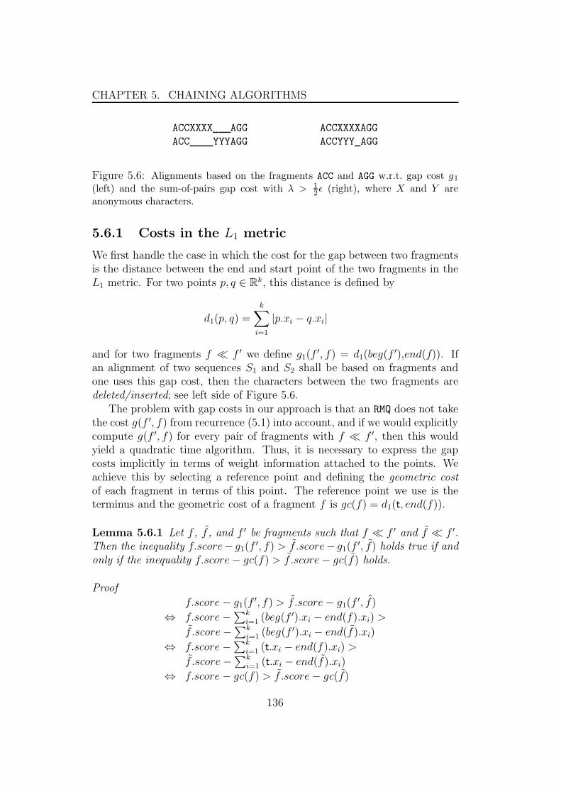
CHAPTER 5. CHAINING ALGORITHMS
ACCXXXX AGG
ACC YYYAGG
ACCXXXXAGG
ACCYYY AGG
Figure 5.6: Alignments based on the fragments ACC and AGG w.r.t. gap cost g1
(left) and the sum-of-pairs gap cost with λ > 12ε (right), where X and Y are
anonymous characters.
5.6.1 Costs in the L1 metric
We first handle the case in which the cost for the gap between two fragmentsis the distance between the end and start point of the two fragments in theL1 metric. For two points p, q ∈ R
k, this distance is defined by
d1(p, q) =
k∑
i=1
|p.xi − q.xi|
and for two fragments f � f ′ we define g1(f′, f) = d1(beg(f ′),end(f)). If
an alignment of two sequences S1 and S2 shall be based on fragments andone uses this gap cost, then the characters between the two fragments aredeleted/inserted; see left side of Figure 5.6.
The problem with gap costs in our approach is that an RMQ does not takethe cost g(f ′, f) from recurrence (5.1) into account, and if we would explicitlycompute g(f ′, f) for every pair of fragments with f � f ′, then this wouldyield a quadratic time algorithm. Thus, it is necessary to express the gapcosts implicitly in terms of weight information attached to the points. Weachieve this by selecting a reference point and defining the geometric costof each fragment in terms of this point. The reference point we use is theterminus and the geometric cost of a fragment f is gc(f) = d1(t, end(f)).
Lemma 5.6.1 Let f , f , and f ′ be fragments such that f � f ′ and f � f ′.Then the inequality f.score− g1(f
′, f) > f.score− g1(f′, f) holds true if and
only if the inequality f.score − gc(f) > f.score − gc(f) holds.
Proof
f.score − g1(f′, f) > f.score − g1(f
′, f)
⇔ f.score − ∑k
i=1 (beg(f ′).xi − end(f).xi) >
f.score − ∑k
i=1 (beg(f ′).xi − end(f).xi)
⇔ f.score − ∑k
i=1 (t.xi − end(f).xi) >
f.score − ∑k
i=1 (t.xi − end(f).xi)
⇔ f.score − gc(f) > f.score − gc(f)
136
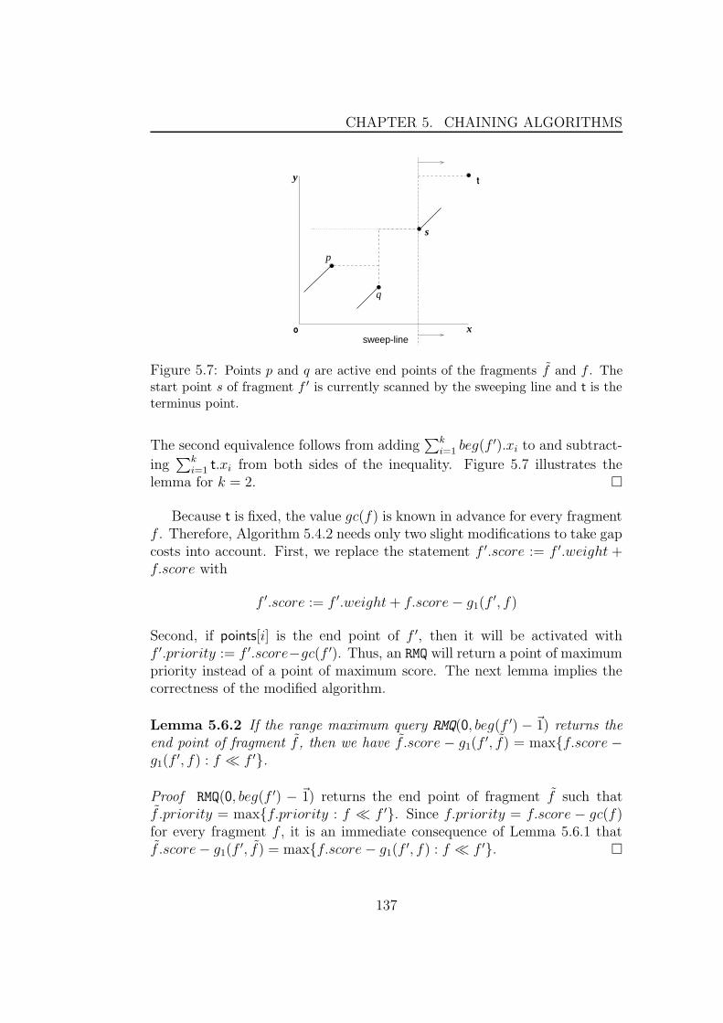
CHAPTER 5. CHAINING ALGORITHMS
sweep-line
ty
xo
s
q
p
Figure 5.7: Points p and q are active end points of the fragments f and f . Thestart point s of fragment f ′ is currently scanned by the sweeping line and t is theterminus point.
The second equivalence follows from adding∑k
i=1 beg(f ′).xi to and subtract-
ing∑k
i=1 t.xi from both sides of the inequality. Figure 5.7 illustrates thelemma for k = 2. �
Because t is fixed, the value gc(f) is known in advance for every fragmentf . Therefore, Algorithm 5.4.2 needs only two slight modifications to take gapcosts into account. First, we replace the statement f ′.score := f ′.weight +f.score with
f ′.score := f ′.weight + f.score − g1(f′, f)
Second, if points[i] is the end point of f ′, then it will be activated withf ′.priority := f ′.score−gc(f ′). Thus, an RMQ will return a point of maximumpriority instead of a point of maximum score. The next lemma implies thecorrectness of the modified algorithm.
Lemma 5.6.2 If the range maximum query RMQ(0, beg(f ′) − ~1) returns theend point of fragment f , then we have f .score − g1(f
′, f) = max{f.score −g1(f
′, f) : f � f ′}.
Proof RMQ(0, beg(f ′) − ~1) returns the end point of fragment f such thatf .priority = max{f.priority : f � f ′}. Since f.priority = f.score − gc(f)for every fragment f , it is an immediate consequence of Lemma 5.6.1 thatf .score − g1(f
′, f) = max{f.score − g1(f′, f) : f � f ′}. �
137
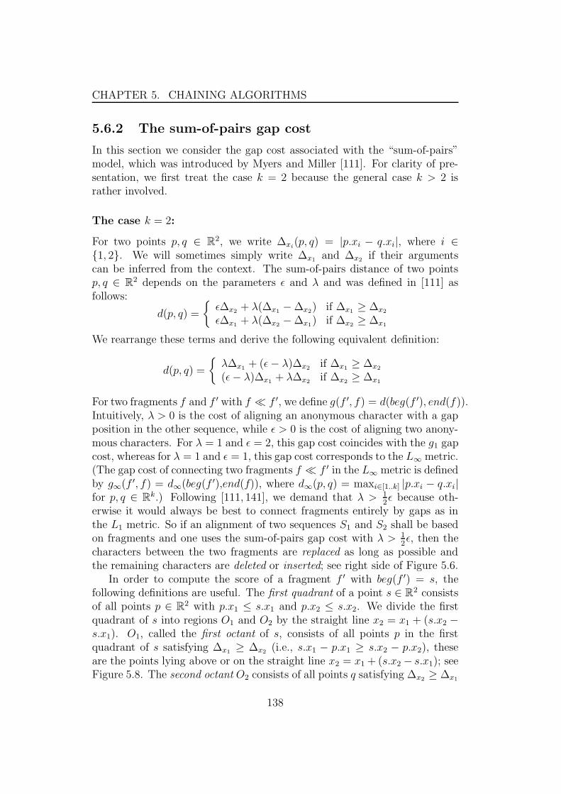
CHAPTER 5. CHAINING ALGORITHMS
5.6.2 The sum-of-pairs gap cost
In this section we consider the gap cost associated with the “sum-of-pairs”model, which was introduced by Myers and Miller [111]. For clarity of pre-sentation, we first treat the case k = 2 because the general case k > 2 israther involved.
The case k = 2:
For two points p, q ∈ R2, we write ∆xi
(p, q) = |p.xi − q.xi|, where i ∈{1, 2}. We will sometimes simply write ∆x1 and ∆x2 if their argumentscan be inferred from the context. The sum-of-pairs distance of two pointsp, q ∈ R
2 depends on the parameters ε and λ and was defined in [111] asfollows:
d(p, q) =
{
ε∆x2 + λ(∆x1 − ∆x2) if ∆x1 ≥ ∆x2
ε∆x1 + λ(∆x2 − ∆x1) if ∆x2 ≥ ∆x1
We rearrange these terms and derive the following equivalent definition:
d(p, q) =
{
λ∆x1 + (ε − λ)∆x2 if ∆x1 ≥ ∆x2
(ε − λ)∆x1 + λ∆x2 if ∆x2 ≥ ∆x1
For two fragments f and f ′ with f � f ′, we define g(f ′, f) = d(beg(f ′), end(f)).Intuitively, λ > 0 is the cost of aligning an anonymous character with a gapposition in the other sequence, while ε > 0 is the cost of aligning two anony-mous characters. For λ = 1 and ε = 2, this gap cost coincides with the g1 gapcost, whereas for λ = 1 and ε = 1, this gap cost corresponds to the L∞ metric.(The gap cost of connecting two fragments f � f ′ in the L∞ metric is definedby g∞(f ′, f) = d∞(beg(f ′),end(f)), where d∞(p, q) = maxi∈[1..k] |p.xi − q.xi|for p, q ∈ R
k.) Following [111, 141], we demand that λ > 12ε because oth-
erwise it would always be best to connect fragments entirely by gaps as inthe L1 metric. So if an alignment of two sequences S1 and S2 shall be basedon fragments and one uses the sum-of-pairs gap cost with λ > 1
2ε, then the
characters between the two fragments are replaced as long as possible andthe remaining characters are deleted or inserted; see right side of Figure 5.6.
In order to compute the score of a fragment f ′ with beg(f ′) = s, thefollowing definitions are useful. The first quadrant of a point s ∈ R
2 consistsof all points p ∈ R
2 with p.x1 ≤ s.x1 and p.x2 ≤ s.x2. We divide the firstquadrant of s into regions O1 and O2 by the straight line x2 = x1 + (s.x2 −s.x1). O1, called the first octant of s, consists of all points p in the firstquadrant of s satisfying ∆x1 ≥ ∆x2 (i.e., s.x1 − p.x1 ≥ s.x2 − p.x2), theseare the points lying above or on the straight line x2 = x1 + (s.x2 − s.x1); seeFigure 5.8. The second octant O2 consists of all points q satisfying ∆x2 ≥ ∆x1
138
CHAPTER 5. CHAINING ALGORITHMS
t
s
sweep-line
y
xo
pO
O
q
2
1
Figure 5.8: The first quadrant of a point s is divided into two octants O1 and O2.
(i.e., s.x2 − q.x2 ≥ s.x1 − q.x1), these are the points lying below or on thestraight line x2 = x1+(s.x2−s.x1). Then f ′.score = f ′.weight+max{v1, v2},where vi = max{f.score − g(f ′, f) : f � f ′ and end(f) lies in octant Oi},for i ∈ {1, 2}.
However, our chaining algorithms rely on RMQs, and these work only fororthogonal regions, not for octants. For this reason, we will make use ofthe octant-to-quadrant transformations of Guibas and Stolfi [61]. The trans-formation T1 : (x1, x2) 7→ (x1 − x2, x2) maps the first octant to a quad-rant. More precisely, point T1(p) is in the first quadrant of T1(s) if andonly if p is in the first octant of point s.2 Similarly, for the transformationT2 : (x1, x2) 7→ (x1, x2 − x1), point q is in the second octant of point s if andonly if T2(q) is in the first quadrant of T2(s). By means of these transfor-mations, we can apply the same techniques as in the previous sections. Wejust have to define the geometric cost properly. The following lemma showshow to choose the geometric cost gc1 for points in the first octant O1. Ananalogous lemma holds for points in the second octant.
Lemma 5.6.3 Let f , f , and f ′ be fragments such that f � f ′ and f � f ′.If end(f) and end(f) lie in the first octant of beg(f ′), then f.score−g(f ′, f) >f.score − g(f ′, f) if and only if f.score − gc1(f) > f.score − gc1(f), wheregc1(f) = λ∆x1(t, end(f)) + (ε − λ)∆x2(t, end(f)) for any fragment f .
Proof Similar to the proof of Lemma 5.6.1. �
2Observe that the transformation may yield points with negative coordinates, but it iseasy to overcome this obstacle by an additional transformation (a translation). Hence wewill skip this minor problem.
139

CHAPTER 5. CHAINING ALGORITHMS
In Subsection 5.6.1 there was only one geometric cost gc, but here wehave to take two different geometric costs gc1 and gc2 into account. To copewith this problem, we need two data structures D1 and D2, where Di storesthe set of points
{Ti(end(f)) | f is a fragment}If we encounter the end point of fragment f ′ in Algorithm 5.4.2, then weactivate point T1(end(f ′)) in D1 with priority f ′.score − gc1(f
′) and pointT2(end(f ′)) in D2 with priority f ′.score − gc2(f
′). If we encounter the startpoint of fragment f ′, then we launch two range maximum queries, namelyRMQ(0, T1(beg(f ′)−~1)) in D1 and RMQ(0, T2(beg(f ′)−~1)) in D2. If the first RMQreturns T1(end(f1)) and the second returns T2(end(f2)), then fi is a fragmentof highest priority in Di, 1 ≤ i ≤ 2, such that Ti(end(fi)) � Ti(beg(f ′)).Because a point p is in the octant Oi of point beg(f ′) if and only if Ti(p) isin the first quadrant of Ti(beg(f ′)), it follows that fi is a fragment such thatits priority fi.score − gci(fi) is maximal in octant Oi. Therefore, accordingto Lemma 5.6.3, the value vi = fi.score − g(f ′, fi) is maximal in octant Oi.Hence, if v1 > v2, then we set f ′.prec = f1 and f ′.score := f ′.weight + v1.Otherwise, we set f ′.prec = f2 and f ′.score := f ′.weight + v2.
For the sum-of-pairs gap cost, the two-dimensional chaining algorithmruns in O(m log m log log m) time and O(m log m) space because of the two-dimensional RMQs required for the transformed points. This is in sharp con-trast to gap costs in the L1-metric, where we merely need one-dimensionalRMQs.
The case k > 2:
In this case, the sum-of-pairs gap cost is defined for fragments f � f ′ by
gsop(f′, f) =
∑
0≤i<j≤k
g(f ′i,j, fi,j)
where f ′i,j and fi,j are the two-dimensional fragments consisting of the ith
and jth component of f ′ and f , respectively. For example, in case of k = 3,let s = beg(f ′) and p = end(f) and assume that ∆x1(s, p) ≥ ∆x2(s, p) ≥∆x3(s, p). In this case, we have gsop(f
′, f) = 2λ∆x1 + ε∆x2 + (ε − λ)2∆x3
because g(f ′1,2, f1,2) = λ∆x1 + (ε − λ)∆x2, g(f ′
1,3, f1,3) = λ∆x1 + (ε − λ)∆x3,and g(f ′
2,3, f2,3) = λ∆x2 +(ε−λ)∆x3 . By contrast, if ∆x1 ≥ ∆x3 ≥ ∆x2 , thenthe equality gsop(f
′, f) = 2λ∆x1 + (ε − λ)2∆x2 + ε∆x3 holds.In general, each of the k! permutations π of 1, . . . , k yields a hyper-region
Rπ defined by ∆xπ(1)≥ ∆xπ(2)
≥ · · · ≥ ∆xπ(k)in which a specific formula for
gsop(f′, f) holds. That is, in order to obtain the score of a fragment f ′, we
140

CHAPTER 5. CHAINING ALGORITHMS
must compute f ′.score = f ′.weight+max{vπ | π is a permutation of 1, . . . , k},where
vπ = max{f.score − gsop(f′, f) : f � f ′ and end(f) lies in Rπ}
Because our RMQ-based approach requires orthogonal regions, each of thesehyper-regions Rπ of s must be transformed into the first hyper-corner ofsome point s. The first hyper-corner of a point s ∈ R
k is the k-dimensionalanalogue to the first quadrant of a point in R
2. It consists of all points p ∈ Rk
with p.xi ≤ s.xi for all 1 ≤ i ≤ k (note that there are 2k hyper-corners). Wedescribe the generalization of the octant-to-quadrant transformations for thecase k = 3. The extension to the case k > 3 is obvious. There are 3!hyper-regions, hence 6 transformations:
∆x1 ≥ ∆x2 ≥ ∆x3 : T1(x1, x2, x3) = (x1 − x2, x2 − x3, x3)
∆x1 ≥ ∆x3 ≥ ∆x2 : T2(x1, x2, x3) = (x1 − x3, x2, x3 − x2)
∆x2 ≥ ∆x1 ≥ ∆x3 : T3(x1, x2, x3) = (x1 − x3, x2 − x1, x3)
∆x2 ≥ ∆x3 ≥ ∆x1 : T4(x1, x2, x3) = (x1, x2 − x3, x3 − x1)
∆x3 ≥ ∆x1 ≥ ∆x2 : T5(x1, x2, x3) = (x1 − x2, x2, x3 − x1)
∆x3 ≥ ∆x2 ≥ ∆x1 : T6(x1, x2, x3) = (x1, x2 − x1, x3 − x2)
In what follows, we will focus on the particular case where π is the identitypermutation. The hyper-region corresponding to the identity permutationwill be denoted by R1 and its transformation by T1. The other permutationsare numbered in an arbitrary order and are handled similarly.
Lemma 5.6.4 Point p ∈ Rk is in hyper-region R1 of point s if and only if
T1(p) is in the first hyper-corner of T1(s), where T1(x1, x2, . . . , xk) = (x1 −x2, x2 − x3, . . . , xk−1 − xk, xk).
Proof T1(p) is in the first hyper-corner of T1(s)
⇔ T1(s).xi ≥ T1(p).xi for all 1 ≤ i ≤ k⇔ s.xi − s.xi+1 ≥ p.xi − p.xi+1 and s.xk ≥ p.xk for all 1 ≤ i < k⇔ (s.x1 − p.x1) ≥ (s.x2 − p.x2) ≥ · · · ≥ (s.xk − p.xk)⇔ ∆x1(s, p) ≥ ∆x2(s, p) ≥ · · · ≥ ∆xk
(s, p)
The last statement holds if and only if p is in hyper-region R1 of s. �
For each hyper-region Rj, we compute the corresponding geometric costgcj(f) of every fragment f . Note that for every index j a k-dimensionalanalogue to Lemma 5.6.3 holds. Furthermore, for each transformation Tj, we
141

CHAPTER 5. CHAINING ALGORITHMS
keep a data structure Dj that stores the transformed end points Tj(end(f))of all fragments f . Algorithm 5.6.5 generalizes the 2-dimensional chainingalgorithm described above to k dimensions.
Algorithm 5.6.5 k-dim. chaining of n fragments w.r.t. the sum-of-pairs gapcost
Sort all start and end points of the n fragments in ascending order w.r.t.their x1 coordinate and store them in the array points; because we includethe end point of the origin and the start point of the terminus, there are2n + 2 points.for j := 1 to k!
apply transformation Tj to the end points of the fragments and store theresulting points as inactive in the k-dimensional data structure Dj
for i := 1 to 2n + 2if points[i] is the start point of fragment f ′ then
maxRMQ := −∞for j := 1 to k!
q := RMQ(0, Tj(points[i] −~1)) in Dj
determine the fragment fq with Tj(end(fq)) = qmaxRMQ := max{maxRMQ, fq.score − gsop(f
′, fq)}if fq.score − gsop(f
′, fq) = maxRMQ then f := fq
f ′.prec := ff ′.score := f ′.weight + maxRMQ
else /? points[i] is end point of a fragment f ′ ?/for j := 1 to k!
activate Tj(points[i]) in Dj with priority f ′.score − gcj(f′)
For every start point beg(f ′) of a fragment f ′, Algorithm 5.6.5 searches for afragment f in the first hyper-corner of beg(f ′) such that f.score− gsop(f
′, f)is maximal. This entails k! RMQs because the first hyper-corner is divided intok! hyper-regions. Analogously, for every end point end(f ′) of a fragment f ′,Algorithm 5.6.5 performs k! activation operations. Therefore, the total timecomplexity of Algorithm 5.6.5 is O(k! m logk−1 m log log m) and its spacerequirement is O(k! m logk−1 m). This result improves the running time ofMyers and Miller’s algorithm [111] by a factor log m
log log m.
If the kd -tree is used instead of the range tree, the algorithms take
O(k! m2− 1k−1 ) time and O(m) space in the worst case, where k > 2.
As already mentioned in the Chapter 3, software-tools that computeglobal alignments of large sequences use the anchor-based strategy to copewith the huge amount of data. Obviously, Algorithm 5.4.2 solves the chainingphase of the anchor-based strategy in sub-quadratic time. The incorporation
142
CHAPTER 5. CHAINING ALGORITHMS
of gap costs turns the algorithm into a practical tool for computing globalalignments of whole genomes. Its extension to the higher-dimensional casemakes it possible to compare multiple genomes simultaneously.
5.7 Local chaining: a basic variation
Global alignments are invaluable in comparing genomes of closely relatedspecies. For diverged genomic sequences, where genome rearrangements oc-curs, a global alignment strategy, however, is likely predestined to failure forhaving to align unrelated regions in an end-to-end colinear approach. In thiscase, local alignments are the strategy of choice. The anchor based strategycan be used to find local regions of similarity in large genomic DNA sequences.More precisely, one first computes fragments between the given genomes. Inthe second phase, instead of computing a highest-scoring global chain ofcolinear non-overlapping fragments, we compute significant local chains ofcolinear non-overlapping fragments. (A local chain is said to be significant ifits score exceeds a user-defined threshold.) Under stringent thresholds, signif-icant local chains of colinear non-overlapping fragments represent candidateregions of conserved synteny. If one aligns these individually, one gets goodlocal alignments. As we shall see in the next chapter, the automatic identi-fication of regions of similarity is a first step toward an automatic detectionof genome rearrangements.
In the previous sections, we have tackled the global chaining problem,which asks for an optimal chain starting at the origin 0 and ending at termi-nus t. However, in searching for local similarities in genomic sequences, oneis interested in chains that can start and end with arbitrary fragments. If weremove the restriction that a chain must start at the origin and end at theterminus, we get the local chaining problem; see Figure 5.9.
Definition 5.7.1 Given m weighted fragments and a gap cost function g,the local fragment-chaining problem is to determine a chain of highest score≥ 0. Such a chain will be called optimal local chain.
Note that if g is the constant function 0, then an optimal local chainmust also be an optimal global chain, and vice versa. Our solution to thelocal chaining problem is a variant of the global chaining algorithm. For easeof presentation, we will use gap costs corresponding to the L1 metric (seeSubsection 5.6.1), but the approach also works with the g∞ and sum-of-pairsgap cost (see Section 5.6.2).
143

CHAPTER 5. CHAINING ALGORITHMS
(b)(a)
o g
g
1
2
2
3
4
5 9
g
g1
2
1
2
4 5
6
7 8
9
1 4 67 8
3 6
1
7
8
Figure 5.9: Computation of local chains of colinear non-overlapping fragments.The optimal local chain is composed of the fragments 1, 4, and 6. Another signif-icant local chain consists of the fragments 7 and 8.
Definition 5.7.2 Let f ′.score = max{score(C) : C is a chain ending withf ′}. A chain C ending with f ′ and satisfying f ′.score = score(C) will becalled optimal chain ending with f ′.
Lemma 5.7.3 The following equality holds:
f ′.score = f ′.weight + max({0} ∪ {f.score − g1(f′, f) : f � f ′}) (5.2)
Proof Let C ′ = f1, f2, . . . , f`, f′ be an optimal chain ending with f ′, that
is, score(C ′) = f ′.score. Because the chain that solely consists of frag-ment f ′ has score f ′.weight ≥ 0, we must have score(C ′) ≥ f ′.weight. Ifscore(C ′) = f ′.weight, then f.score−g1(f
′, f) ≤ 0 for every fragment f thatprecedes f ′, because otherwise it would follow score(C ′) > f ′.weight. Henceequality (5.2) holds in this case. So suppose score(C ′) > f ′.weight. Clearly,score(C ′) = f ′.weight + score(C) − g1(f
′, f`), where C = f1, f2, . . . , f`. It isnot difficult to see that C must be an optimal chain that is ending withf` because otherwise C ′ would not be optimal. Therefore, score(C ′) =f ′.weight + f`.score− g1(f
′, f`). If there were a fragment f that precedes f ′
such that f.score− g1(f′, f) > f`.score− g1(f
′, f`), then it would follow thatC ′ is not optimal. We conclude that equality (5.2) holds. �
With the help of Lemma 5.7.3, we obtain an algorithm that solves thelocal chaining problem.
Algorithm 5.7.4 Finding an optimal local chain based on RMQ
144
CHAPTER 5. CHAINING ALGORITHMS
for every fragment f ′ do begin
determine f such that f .score − g1(f′, f) = max{f.score − g1(f
′, f) : f� f ′}max := max{0, f .score − g1(f
′, f)}if max > 0 then f ′.prec := f else f ′.prec := NULLf ′.score := f ′.weight + max
end
determine a fragment f such that f .score = max{f.score : f is a fragment}report an optimal local chain by tracing back the pointers from f .prec untila fragment f with f.prec = NULL is reached
It is not difficult to verify that we can use the techniques of the previoussections to solve the local fragment-chaining problem in the same time andspace complexities as the global fragment-chaining problem.
Algorithm 5.7.4 can easily be modified, so that it can report all chainswhose score exceeds some threshold T (in Algorithm 5.7.4, instead of deter-mining a fragment f of highest score, one determines all fragments whosescore exceeds T ). Such chains will be called significant local chains; see Fig-ure 5.9. In this case, however, an additional problem arises: Several chainscan share one or more fragments, so that the output can be quite complex.To avoid this, local chains are partitioned into equivalence classes by thestarting fragment of the chain [38, 70]. Two local chains belong to the sameclass if and only if they begin with the same fragment. In Figure 5.9, thelocal chains {7, 8} and {7, 9} compose an equivalent class because they sharethe fragment {7}. Instead of reporting all the chains in an equivalence class,only the one with the highest-score is reported as a representative chain ofthat class. In Figure 5.9, for example, the two chains {1, 4, 6} and {7, 8}are reported. As outlined before, under stringent thresholds, significant localchains of colinear non-overlapping fragments represent candidate regions ofconserved synteny. Furthermore, the automatic identification of regions ofsimilarity is a first step toward an automatic detection of genome rearrange-ments. In the next chapter, we show how our local chaining method is usedto detect genome rearrangements such as transpositions and inversions.
5.8 Variations
Global and local chaining algorithms represent the core ideas in the anchorbased strategy. However, additional requirements are necessary when dealingwith real genomic sequences and when addressing other comparative genomictasks. In this section, we introduce two important variations of the chaining
145
CHAPTER 5. CHAINING ALGORITHMS
algorithms. The first is the inclusion of gap constraints and the second is thecDNA/EST mapping.
5.8.1 Including gap constrains
In Algorithm 5.7.4, the local chains are allowed to grow as long as the scoreis positive. This can cause the problem that unrelated matches, despite lyingfar away, may be appended at the tail of a chain. To avoid such cases, it isdesirable to constrain the gap between the successive fragments of a chain.
To constrain the gap between the fragments, the RMQ is restricted to aregion R(t1, t2) bounded by the start point of a fragment t2 and a pointt1 such that t2.xi − t1.xi ≤ gap const, for all 1 ≤ i ≤ k, where gap constdenotes the allowed gap length. Because this restriction is k dimensionaland we use (k − 1) dimensional RMQ, we need to deactivate all the pointsp′ such that p′.x1 < t1.x1. Hence, we can execute RMQ(t1, t2 − ~1), wheret1 = (t1.x2, . . . , t1.xk) and t2 = (t2.x2, . . . , t2.xk). Algorithm 5.8.1 describeshow to include gap constraints in the local chaining algorithm.
Algorithm 5.8.1 Local chaining with gap constraints
Sort all start and end points of the m fragments in ascending order w.r.t.their x1 coordinate and store them in the array points; the points contains2m points.Store all end points of the fragments (ignoring their x1 coordinate) asinactive (in the k − 1-dimensional) data structure D.for i := 1 to 2m
deactivate all end points points[j], such that j < i andpoints[i].x1 − points[j].x1 > gap constif points[i] is the start point of fragment f ′ then
t1 = (points[i].x2 − gap const, . . . , points[i].xk − gap const)t2 = (points[i].x2, . . . , points[i].xk)
q := RMQ(t1, t2 −~1)determine the fragment f with end(f) = qif f 6= ⊥
max := max{0, f .score − g1(f′, f)}
if max > 0 then f ′.prec := f else f ′.prec := NULLf ′.score := f ′.weight + max
else /? points[i] is end point of a fragment f ′ ?/f ′.priority := f ′.score − gc(f ′)activate (points[i].x2, . . . points[i].xk) in D /? with priority f ′.priority ?/
146
CHAPTER 5. CHAINING ALGORITHMS
The time complexity of this algorithm depends on the data structure Dsupporting the three operations RMQ, activation, and deactivation.
For two dimensions, we can use the dynamic or semi dynamic prioritysearch tree described before. Allowing for an arbitrary rectangular rangesearch can be done in the same time complexity [122]. A point is deactivatedin the semi-dynamic version by simply updating its score with the value −∞,while in the dynamic version it is deleted. The deactivation can be done forboth versions of the priority search tree in O(log m). Thus, the complexityof the algorithm using either versions of the priority tree is O(m log m).
Unfortunately, this approach does not hold for two dimensional chainingwhere the RMQ is based on a priority queue supporting the operations delete,predecessor, successor (Subsection 5.4.2, Alternative 3). The reason forthis is that the RMQ is no longer in the range R(0, p), q is a start point of afragment. More specifically, the data structure D, which is a priority queue,maintains a list of end points 0 ≤ qi ≤ n such that 0 ≤ q1 ≤ · · · ≤ q` ≤ n andq1.score ≤ · · · ≤ q`.score. If there is a point qz > qy but qy.score > qz.score,then point qz will be deleted. This deletion is problematic if we perform aquery with point qx > qz > qy. In this case we obtain qy = predecessor(qx)because qz is deleted. If q.y is in the range within a gap constraint, then itwill be connected to qx. Otherwise, it is not connected, and consequentlyno point else in the data structure can be connected to qx. This is despitethe fact that qz does not violate the gap constraint and could have beenconnected to qx.
For higher dimensions and D being the semi-dynamic range tree, thecomplexity of the algorithm becomes a little bit higher than the one withoutgap constraints. The reason for this is that the range search is no longer inthe range R(0, p) so that the one dimensional priority queue can be used inthe last dimension of the range tree; this follows from the same argumentsmentioned above for the 1D RMQ using these operations. In this case, wecannot profit from the fractional cascading and we have to use the originalrange tree so that the last dimension is enhanced with priority search treessupporting RMQ, activation, and deactivation. This makes the complexityof these operations for a d-dimensional point O(logd m). That is, the timecomplexity of Algorithm 5.8.1 becomes O(m logk−1 m). The space complexityremains unchanged, i.e., O(m logk−2 m).
The usage of a dynamic range tree without fractional cascading yieldsan algorithm with the same time complexity. This is because the inser-tion/deletion of a point takes O(logd m) time, which is the same as thatof an RMQ. A practical advantage of using the dynamic range tree in thisalgorithm is that the points that are out of the RMQ range are deleted. Adisadvantage is that the dynamic version is too complicated to implement.
147
CHAPTER 5. CHAINING ALGORITHMS
If the semi-dynamic kd -tree is used, the complexity of the RMQ, activation,and deactivation will be the same. The usage of a dynamic version of thekd -tree is also possible, but it leads to a tradeoff. On the one hand, the spaceconsumption is reduced in practice, since the points that are in the queryrange are maintained while those that are out of the RMQ range are deleted.On the other hand, answering an RMQ over a dynamic kd -tree has a time
complexity that is higher with factor log1d m than that of the semi-dynamic
tree, which yields an algorithm with higher time complexity. Moreover, thedynamic kd -tree is more complicated than the semi-dynamic one.
5.8.2 cDNA/EST mapping
cDNA (complementary or copy DNA) is DNA obtained from mRNA (mes-senger RNA) through reverse transcription. Recalling from Chapter 2 thatthe mRNA stemming from eukaryotes is a complementary sequence to a geneafter the introns being spliced out, the cDNA is then the original sequence ofthe exons of the gene; see Figure 5.10. cDNA can be prepared in the lab byfirst separating the mRNA content of a cell. Then the reverse transcriptaseenzyme, which uses the mRNAs as templates for producing the cDNAs, is ap-plied. Each cDNA is finally separated and sequenced. To reduce the costs,not each cDNA is sequenced. Rather parts of it called ESTs (ExpressedSequence Tags) are prepared and sequenced. The problem of cDNA/ESTmapping is to locate the gene (and if possible determine its exon/intronstructure) on the genome from which the cDNA/EST was derived. A precisemapping allows further analysis such as detecting gene splice variants, find-ing regulatory elements, and studying the gene distribution w.r.t. functionalconstrains.
As cDNA lacks the introns that are contained in the DNA sequence fromwhich it was derived, gaps should not be penalized in this application. If wemap the cDNA/EST to the location of a certain single gene, then we canuse the global chaining algorithm without gap costs presented in Section 5.4.However, if we map a cDNA/EST database to a whole genome or even to alarge part of a genome, gap constraints have to be incorporated. There aretwo essential reasons: First, to avoid that an exon is chained to a spuriousrandom match that is very far away. Second, to be able to detect repeatedgenes and correctly assemble them. Including the gap constraint requirementyields an algorithm that is a variation of the local chaining algorithm withgap constraints, where the gaps are not penalized. The value gap const istypically selected such that it is larger than the estimated length of thelongest intron of the studied genome.
148

CHAPTER 5. CHAINING ALGORITHMS
exon 1 exon 3exon 2
exon 2 exon 3
intron intron
exon 1cDNA
Genome
Figure 5.10: cDNA mapped to a genomic sequence.
5.9 Related problems
This section handles two very related problems of the chaining algorithms.Although these problems are well addressed in previous works, we mentionthem here to provide the reader with a thorough view of this area of research,and because some of the algorithms that solve these problems are integratedin our software too CHAINER presented in the next chapter.
5.9.1 1-dimensional chaining
In 1-dimensional chaining, the fragments are 1-dimensional intervals on thex axis and the optimal global chain is a chain of non-overlapping intervals.Clearly, it is superfluous to mention “colinearity”, because any two non-overlapping 1-dimensional fragments are colinear. The following algorithmsolves the 1-dimensional chaining problem without considering gap costs.To avoid confusion between fragments composed of matched segments (k-dimensional fragments), we denote a 1-dimensional fragment by I (standingfor interval) instead of f .
Algorithm 5.9.1 Global 1-dimensional chaining
Sort all start and end points of the m fragments (intervals) in ascendingorder and store them in the array points;Imax := 0
for i := 1 to 2mif points[i] is the start point of a fragment I then
I.prec := Imax
I.score := I.weight + Imax.scoreelse /? points[i] is end point of an interval ?/
determine the fragment I with I.end = points[i]if I.score > Imax.score then Imax := I
In the algorithm, Imax denotes the fragment (interval) that has highest scoreamong all fragments already scanned. Consequently, upon the termination
149

CHAPTER 5. CHAINING ALGORITHMS
of the algorithm, it is the last fragment in an optimal global chain. Notingthat I.prec denotes a field that stores the preceding fragment of I in a chain,we obtain an optimal global chain by following the back-pointers from Imax
to the origin 0. It is easy to see that this algorithm is dominated by thesorting procedure, which takes O(m log m) time.
As applications, this algorithm can be used to compute the single coverageof one genome w.r.t. another and to compute the transformation distance be-tween two genomes. The single coverage problem was introduced by Schwartzet al. [125], and the algorithm that solves it was implemented in PipMakeras the single coverage option. Given a set of (2-dimensional) fragments oftwo sequences, the single coverage problem is to find a set of fragments ofmaximum coverage w.r.t. one sequence without overlapping in this sequence.That is, the resulting two dimensional fragments are not necessary colinear(corresponding to transposition) and their segments can overlap in the secondsequence (corresponds to duplication). In other words, every position in thefirst sequence is covered by at most one fragment in the resulting fragmentset, and the number of sequence positions covered by this set is maximal.The single coverage problem can be defined formally as follows.
Definition 5.9.2 We define a binary relation �x on the set of 2-dimensionalfragments by f �x f ′ if and only if end(f).x < beg(f ′).x.
Definition 5.9.3 Given a set F of m fragments, the single coverage prob-lem is to find a subset F ′ = {f1, f2, . . . , f`} of F such that the elementsof F ′ do not overlap on the x-axis (i.e., either fi �x fj or fj �x fi) and∑`−1
i=1(end(fi).x − beg(fi).x) is maximized.
For any 2-dimensional fragment f = (beg(f), end(f)), let the interval If
[beg(f).x, . . . , end(f).x] be the corresponding one dimensional fragment, i.e.,If is the projection of f to the x-axis. Given a set F = {f1, . . . , fm} of 2-dimensional m fragments, it is not difficult to see that a solution to the singlecoverage problem can be found by solving the global 1-dimensional chainingproblem for the set {If1 , . . . , Ifm
}.The transformation distance [134] addresses the question of how two
sequences may be most economically derived from one another by variousgenome rearrangements. As shown in [134], computing the transformationdistance reduces to solving the 1-dimensional global chaining problem, wherethe gap between the fragments are penalized. However, the authors solvedthe problem using a graph-based approach, yielding a procedure that runsin quadratic time. Algorithm 5.9.1 can compute the transformation distanceof fragments in O(m log m) time, but without penalizing the gaps. However,
150
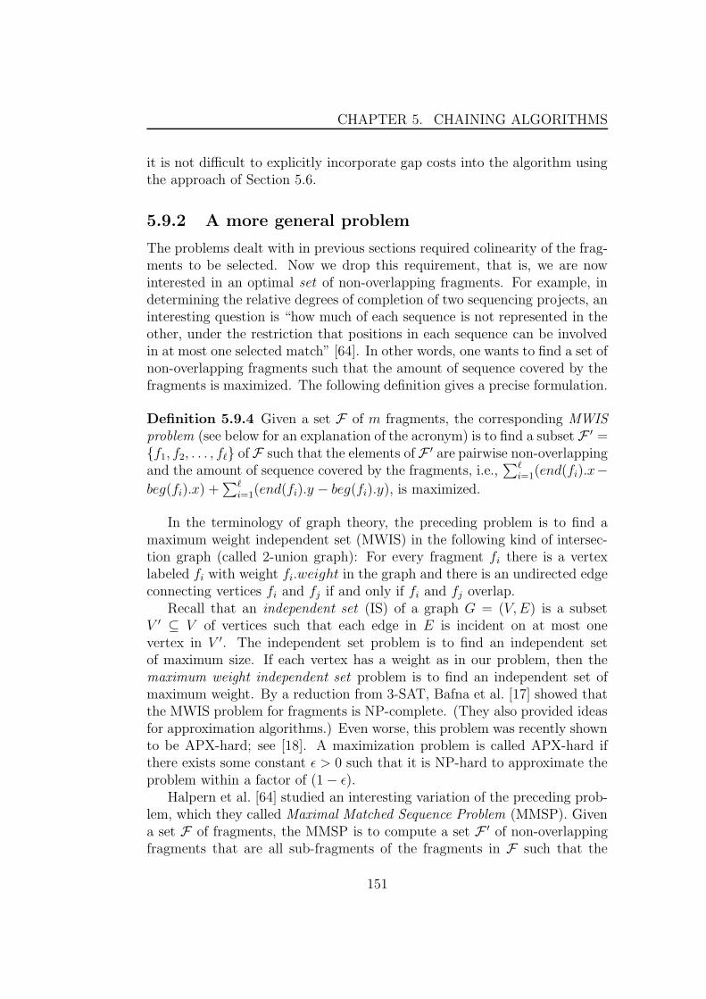
CHAPTER 5. CHAINING ALGORITHMS
it is not difficult to explicitly incorporate gap costs into the algorithm usingthe approach of Section 5.6.
5.9.2 A more general problem
The problems dealt with in previous sections required colinearity of the frag-ments to be selected. Now we drop this requirement, that is, we are nowinterested in an optimal set of non-overlapping fragments. For example, indetermining the relative degrees of completion of two sequencing projects, aninteresting question is “how much of each sequence is not represented in theother, under the restriction that positions in each sequence can be involvedin at most one selected match” [64]. In other words, one wants to find a set ofnon-overlapping fragments such that the amount of sequence covered by thefragments is maximized. The following definition gives a precise formulation.
Definition 5.9.4 Given a set F of m fragments, the corresponding MWISproblem (see below for an explanation of the acronym) is to find a subset F ′ ={f1, f2, . . . , f`} of F such that the elements of F ′ are pairwise non-overlappingand the amount of sequence covered by the fragments, i.e.,
∑`
i=1(end(fi).x−beg(fi).x) +
∑`
i=1(end(fi).y − beg(fi).y), is maximized.
In the terminology of graph theory, the preceding problem is to find amaximum weight independent set (MWIS) in the following kind of intersec-tion graph (called 2-union graph): For every fragment fi there is a vertexlabeled fi with weight fi.weight in the graph and there is an undirected edgeconnecting vertices fi and fj if and only if fi and fj overlap.
Recall that an independent set (IS) of a graph G = (V, E) is a subsetV ′ ⊆ V of vertices such that each edge in E is incident on at most onevertex in V ′. The independent set problem is to find an independent setof maximum size. If each vertex has a weight as in our problem, then themaximum weight independent set problem is to find an independent set ofmaximum weight. By a reduction from 3-SAT, Bafna et al. [17] showed thatthe MWIS problem for fragments is NP-complete. (They also provided ideasfor approximation algorithms.) Even worse, this problem was recently shownto be APX-hard; see [18]. A maximization problem is called APX-hard ifthere exists some constant ε > 0 such that it is NP-hard to approximate theproblem within a factor of (1 − ε).
Halpern et al. [64] studied an interesting variation of the preceding prob-lem, which they called Maximal Matched Sequence Problem (MMSP). Givena set F of fragments, the MMSP is to compute a set F ′ of non-overlappingfragments that are all sub-fragments of the fragments in F such that the
151

CHAPTER 5. CHAINING ALGORITHMS
Figure 5.11: Two fragments fi = (beg(fi), end(fi)) and fj = (beg(fj), end(fj))overlapping on both axes are refined into the three fragments (beg(fi), beg(fj)),(beg(fj), end(fi)), and (end(fi), end(fj)).
amount of sequence covered by the fragments is maximized. Halpern et al.[64] showed that this problem can be solved optimally in polynomial time.The key idea of their solution is to minimally “refine” (subdivide) fragmentsuntil all overlaps between the refined fragments are “resolved”, i.e., the pro-jections of any two refined fragments onto each sequence are either disjointor identical; see Figures 5.11 and 5.12. As a result, solving the MaximalMatched Sequence Problem is reduced to find a maximal weight matching ofa bipartite graph, which can be done in polynomial time.
5.10 Conclusions
In this chapter, we have presented line-sweep algorithms that solve both theglobal and the local fragment-chaining problem of multiple genomes. Fork = 2 genomes, our algorithms take
• O(m log log m) time and O(m) space without gap costs,
• O(m log log m) time and O(m) space for gap costs in the L1 metric,
• O(m log m log log m) time and O(m) space for the sum-of-pairs gap costand for gap costs in the L∞ metric.
If the start and end points of the fragments are not sorted w.r.t. one dimen-sion, then the complexity is dominated, in case of neglecting gap costs andgap costs in the L1 metric, by the sorting procedure, which takes O(m log m).Although our algorithm is higher with a log factor than the one of [50, 138],in case of sum-of-pairs gap cost and for gap costs in the L∞ metric, ouralgorithm is much less complicated and usable in practice. It also has the
152
CHAPTER 5. CHAINING ALGORITHMS
Figure 5.12: Two fragments overlapping on the x-axis but not on the y-axis aresubdivided into four refined fragments.
advantage of incorporating gap constraints, which is not possible in the otheralgorithm.
For k > 2 genomes, our algorithms that are based on the semi-dynamicrange tree take
• O(m logk−2 m log log m) time and O(m logk−2 m) space without gapcosts,
• O(m logk−2 m log log m) time and O(m logk−2 m) space for gap costs inthe L1 metric,
• O(k! m logk−1 m log log m) time and O(k! m logk−1 m) space for thesum-of-pairs gap cost and for gap costs in the L∞ metric.
These results improve upon previous results obtained by Myers and Miller[111]. For gap costs in the L1-metric, we reduced the space complexity by
a log-factor and improved the time complexity by a factor log2 m
log log m. For the
sum-of-pairs gap cost, we improved the time complexity by a factor log m
log log m.
If the semi-dynamic kd -tree is used instead of the range tree, the algo-
rithms take O((k − 1)m2− 1k−1 ) time and O(m) space for gap costs in the
L1 metric. For the sum-of-pairs gap costs, they take O((k!)m2− 1k ) time and
O(k!m) space. It is worth mentioning that we are the first to present acomplexity analysis of the chaining algorithms using the kd -tree.
Although there is a trade-off in theory between the kd -tree and rangetree, our experimental results presented in this chapter shows that the kd -tree is superior in practice to the range tree. Therefore, our software toolCHAINER [5], presented in the next chapter, contains an implementation ofthe chaining algorithms based on the kd -tree. We stress, however, that ouralgorithms can employ any other data structure that supports orthogonalrange-searching.
153

CHAPTER 5. CHAINING ALGORITHMS
We have also shown that on-line chaining can be performed if one usesa dynamic data structure for RMQ, where the points are inserted while thefragments are generated. For k = 2, our algorithms take O(m log log m).For higher dimensions, the complexity of the RMQ using a dynamic kd -tree is,unfortunately, higher than using the respective semi-dynamic version; addto this that the dynamic version is too complicated to implement. To usean efficient dynamic data structure for on-line k dimensional chaining in thesame complexity as using the semi-dynamic data structures remains an openproblem. Moreover, to have a non-complicated implementation of dynamicdata structures and to improve its running time for larger data sets in practiceis a challenging task.
We have also introduced many variations of the chaining algorithms.These variations included chaining with gap constraints and cDNA/ESTmapping. These variations are implemented and integrated in the softwaretool CHAINER to provide efficient solutions to versatile comparative genomictasks.
To provide the reader with a thorough overview of the chaining algo-rithms, we added a section discussing the recent work regarding the 1-dimensional chaining problem and the maximal weight independent set prob-lem on fragments. A solution to the former problem yields the maximumcoverage of one genome w.r.t. another one and it can also yield the trans-formation distance between them. The second problem is addressed whencomparing assemblies of two genomes.
It is worth mentioning that chaining algorithms are also useful in otherapplications. In bioinformatics, they are used in comparing restriction maps[109]; see [62, Section 16.10]. In string processing, they can be used to solvethe longest/heaviest increasing subsequence problem. Moreover, in graphtheory they provide an efficient solution to the maximum weight independentset problem in a k-trapezoid graph that has an application in VLSI design[42, 51]. For more details regarding these additional applications, see [113].
154
Chapter 6
CHAINER: the softwaresystem
In this chapter, we describe the software system CHAINER and demonstratehow it can be used for various comparative genomic tasks, such as comparingcomplete genomes, comparing draft genomes, and cDNA/EST mapping.
6.1 Introduction
In the previous chapters of the thesis, we presented the anchor based strategyand its three phases. In Chapter 4, we introduced the enhanced suffix arrays,and showed how they can be used to generate various kinds of fragmentsefficiently. Then in Chapter 5 we presented our chaining algorithms and theirvariations. In this chapter, we show how these algorithms are integrated ina single system so that they perform various comparative genomic tasks.Figure 6.1 depicts the block diagram of this software system, which we callCHAINER. There are three basic phases:
1. The fragment generation phase. In this phase, we use algorithms basedon the enhanced suffix array for generating these fragments. Frag-ments of the type MEMs (for two genomes) or multiMEMs (for mul-tiple genomes) are the default types of fragments used in the system.However, the system is modular and CHAINER can use any kind offragments generated by any other software tool, as long as they aregiven in the correct input format.
2. The chaining phase. This phase includes, according to the task at hand,the execution of a chaining algorithm taking the fragments generatedin the first phase as an input. There are four procedures: (1) global
155

CHAPTER 6. CHAINER: THE SOFTWARE SYSTEM
> contig 1 2334 bpDescription Files
> conti
> gi genome 1 GCCGCGCGTCGGTCG..
Fragment Generation Chaining
Post−processing PhaseChaining PhaseFragment Generation Phase
Detailed Alignment
Visualization
Draft−finished Comparison
Clustering cDNA/ESTs
Figure 6.1: The input to the fragment generation tool is the set of files containingthe genomes. CHAINER includes extra information in the description files suchas the size of contigs and cDNA/ESTs. The feedback arrows symbolize recursivecalls: It is possible to generate shorter fragments and run CHAINER again or tofurther chain the output chains.
chaining of fragments of two or multiple genomes. (2) local chainingof fragments of two or multiple genomes. (3) High-throughput localchaining of two or multiple draft genomes. (4) High-throughput map-ping of cDNA/EST. The details of these procedures will be given inthe following sections.
3. The post-processing phase. This phase is optional and it is performedaccording to the task at hand. For example, if fragments are generatedto align two genomes and the global chaining algorithm was executed,then a standard dynamic programming algorithm can be called to alignthe regions within and surrounding the fragments of the chain. Later,we will discuss some additional post-processing procedures, when han-dling the respective tasks.
In the block diagram representation of Figure 6.1, there are two feed-back arrows that symbolize the possibilities of repeating the first and secondphases. The first arrow refers to the possibility of repeating the fragmentgeneration phase followed by the chaining phase. This can be done, e.g.,for processing the regions between the anchors of a global chain, where frag-ments of shorter length can be generated in each of these regions and furtherchained. The objective of this repetition is to reduce the regions to be alignedin the third phase using the standard dynamic programming, and accordinglyreduce the whole comparison time. The second feedback arrow refers to thepossibility of repeating the chaining phase. That is, the regions covered bythe chains are dealt with as fragments and chained again. This option can beused, e.g., for improving the global alignment quality. More precisely, instead
156
CHAPTER 6. CHAINER: THE SOFTWARE SYSTEM
of computing a global chain directly over a set of fragments, the followingtwo steps can be done: (1) A local chaining procedure is first executed overthe set of fragments under stringent thresholds. This is done to find local re-gions of high similarity. (2) The resulting local chains are then considered asfragments, and a global chaining procedure is applied to them. The rationaleof dividing the global chaining task into these two steps is to increase thechance that short regions of high similarity are maintained in the alignment.
The following sections of this chapter demonstrate how our system isused to solve various comparative genomic tasks. In Section 6.2, we show howCHAINER is used to find regions of high similarity. We show how our systemdetects genome rearrangement events such as transpositions and inversions.In Section 6.3, we demonstrate how CHAINER is used for computing globalalignments of multiple genomes. In Section 6.4, we present two modes ofcomparing draft genomes. Section 6.5 presents the options of mapping acDNA/EST database to genomic sequences. In Section 6.6, we discuss howthe parameters of the system are selected. Finally, Section 6.7 contains theconclusions, open problems, and future work.
6.2 Finding regions of high similarity
CHAINER delivers regions of high similarity of two or multiple genomes interms of highest-scoring (local) chains of colinear non-overlapping fragments.CHAINER implements the algorithm presented in Section 5.7, where thegap costs are measured in the L1 metric. The significance of a local chainis determined by a user defined threshold T on its score. (As proven inSection 5.7, chains of score > zero are significant per se, but the user maybe interested in certain regions of higher score and want to filter out theothers.) CHAINER has also the option of constraining the gap between thefragments, as presented in Subsection 5.8.1. Inversions can be taken intoaccount by chaining fragments computed between the reverse complementof some genomes and the other genomes. In the following, we present twoexperiments that show how CHAINER was used to detect transpositionsand inversions. Moreover, we present some results obtained for a large scalecomparison between the human and mouse genomes.
6.2.1 Detecting transposition events
In a comparative study [66] of the genomes of M.genitalium (580,074 bp) andM.pneumonia (816,394 bp), it was shown that most of the former genomeis contained in the latter but some large segments are not conserved in or-
157

CHAPTER 6. CHAINER: THE SOFTWARE SYSTEM
der, i.e., there are transposition events. These segments were first identifiedby all gene-to-gene comparisons using BLAST and FASTA after excludingnon-coding regions. This comparison was repeated again in [44] using threemethods applied directly to the DNA sequences of the two genomes withoutdetermining ORFs. In the first method, the two genomes were divided intowindows of 1000 bp. Then all these windows were compared to each otherusing FASTA. In the second method, MUMs of fixed length (25 bp) wereplotted to visually locate the transposed segments. But in both methods thetranspositions were difficult to identify. In the third method, MUMs of differ-ent lengths were gradually generated (starting with the longest MUMs) untilthe transposition pattern could be visually identified. Based on this visual-ization, these segments were manually separated and aligned independentlyusing the program MUMmer.
We ran our program to automatically locate such transpositions. Figure6.2 (left) shows the fragments of the two genomes. These fragments aremaximal exact matches of minimum length of 12 bp. It is obvious that theplot is too noisy to clearly observe the transposed segments. The right partof the figure shows the local chains in a 2D plot. It is clear that the localchaining procedure has filtered out the noise and identified the transposedsegments. To demonstrate the benefit of generating local chains rather thana global one, we also generated the global chain between the two genomesand, as expected, the global chain yielded misleading results in the transposedregions (data not shown). We ran the program with the following parameters:the fragments were weighted by 4 times their lengths, the gap constraintparameter was set to 50 bp, and the score threshold T = 0. (The way in whichthese parameters are chosen will be explained in Section 6.6.) The chainingprocedure was fast: it took about 8 seconds to chain 97176 fragments. Thegeneration of the fragments took less than half a minute. For this, and allcoming, experiments, we used a Pentium III 933 MHz CPU.
6.2.2 Detecting inversions
It was observed in [48] that inversions in bacterial genomes are centeredaround the origin and/or the terminus of replication; see also [71]. Con-sequently, if homologous regions are plotted in two dimensions, then it iseasy to observe that they are shaping an X-pattern centered around the ori-gin and/or the terminus of replication of the two genomes. In [48], thesepatterns were clearly observed in a two dimensional dot plot of homologousproteins of two bacteria. Every dot in this plot corresponded to two proteinswhose similarity is above some specified threshold (the program BLAST wasused for this task). By contrast, it is not easy to observe the pattern when
158
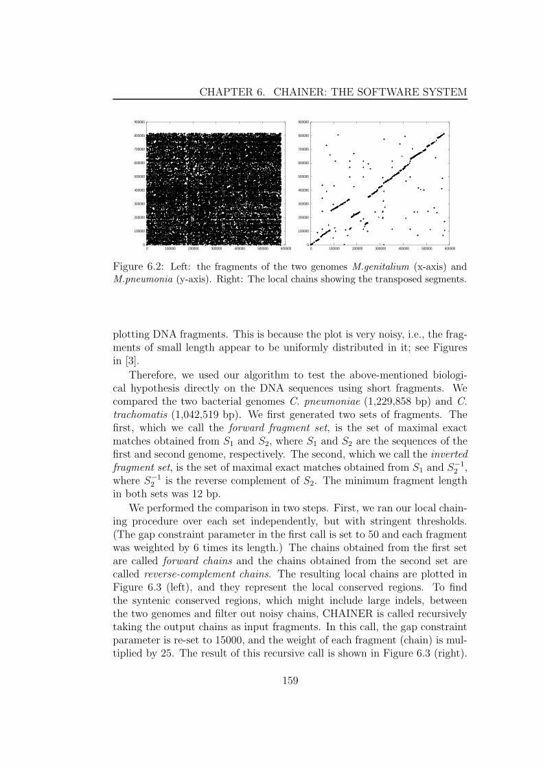
CHAPTER 6. CHAINER: THE SOFTWARE SYSTEM
0
100000
200000
300000
400000
500000
600000
700000
800000
900000
0 100000 200000 300000 400000 500000 600000 0
100000
200000
300000
400000
500000
600000
700000
800000
900000
0 100000 200000 300000 400000 500000 600000
Figure 6.2: Left: the fragments of the two genomes M.genitalium (x-axis) andM.pneumonia (y-axis). Right: The local chains showing the transposed segments.
plotting DNA fragments. This is because the plot is very noisy, i.e., the frag-ments of small length appear to be uniformly distributed in it; see Figuresin [3].
Therefore, we used our algorithm to test the above-mentioned biologi-cal hypothesis directly on the DNA sequences using short fragments. Wecompared the two bacterial genomes C. pneumoniae (1,229,858 bp) and C.trachomatis (1,042,519 bp). We first generated two sets of fragments. Thefirst, which we call the forward fragment set, is the set of maximal exactmatches obtained from S1 and S2, where S1 and S2 are the sequences of thefirst and second genome, respectively. The second, which we call the invertedfragment set, is the set of maximal exact matches obtained from S1 and S−1
2 ,where S−1
2 is the reverse complement of S2. The minimum fragment lengthin both sets was 12 bp.
We performed the comparison in two steps. First, we ran our local chain-ing procedure over each set independently, but with stringent thresholds.(The gap constraint parameter in the first call is set to 50 and each fragmentwas weighted by 6 times its length.) The chains obtained from the first setare called forward chains and the chains obtained from the second set arecalled reverse-complement chains. The resulting local chains are plotted inFigure 6.3 (left), and they represent the local conserved regions. To findthe syntenic conserved regions, which might include large indels, betweenthe two genomes and filter out noisy chains, CHAINER is called recursivelytaking the output chains as input fragments. In this call, the gap constraintparameter is re-set to 15000, and the weight of each fragment (chain) is mul-tiplied by 25. The result of this recursive call is shown in Figure 6.3 (right).
159
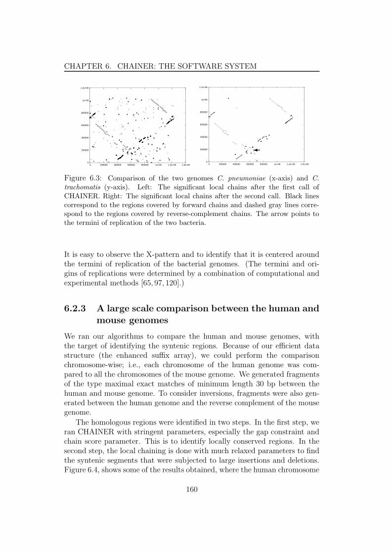
CHAPTER 6. CHAINER: THE SOFTWARE SYSTEM
0
200000
400000
600000
800000
1e+06
1.2e+06
0 200000 400000 600000 800000 1e+06 1.2e+06 1.4e+06 0
200000
400000
600000
800000
1e+06
1.2e+06
0 200000 400000 600000 800000 1e+06 1.2e+06 1.4e+06
�
Figure 6.3: Comparison of the two genomes C. pneumoniae (x-axis) and C.
trachomatis (y-axis). Left: The significant local chains after the first call ofCHAINER. Right: The significant local chains after the second call. Black linescorrespond to the regions covered by forward chains and dashed gray lines corre-spond to the regions covered by reverse-complement chains. The arrow points tothe termini of replication of the two bacteria.
It is easy to observe the X-pattern and to identify that it is centered aroundthe termini of replication of the bacterial genomes. (The termini and ori-gins of replications were determined by a combination of computational andexperimental methods [65, 97, 120].)
6.2.3 A large scale comparison between the human andmouse genomes
We ran our algorithms to compare the human and mouse genomes, withthe target of identifying the syntenic regions. Because of our efficient datastructure (the enhanced suffix array), we could perform the comparisonchromosome-wise; i.e., each chromosome of the human genome was com-pared to all the chromosomes of the mouse genome. We generated fragmentsof the type maximal exact matches of minimum length 30 bp between thehuman and mouse genome. To consider inversions, fragments were also gen-erated between the human genome and the reverse complement of the mousegenome.
The homologous regions were identified in two steps. In the first step, weran CHAINER with stringent parameters, especially the gap constraint andchain score parameter. This is to identify locally conserved regions. In thesecond step, the local chaining is done with much relaxed parameters to findthe syntenic segments that were subjected to large insertions and deletions.Figure 6.4, shows some of the results obtained, where the human chromosome
160
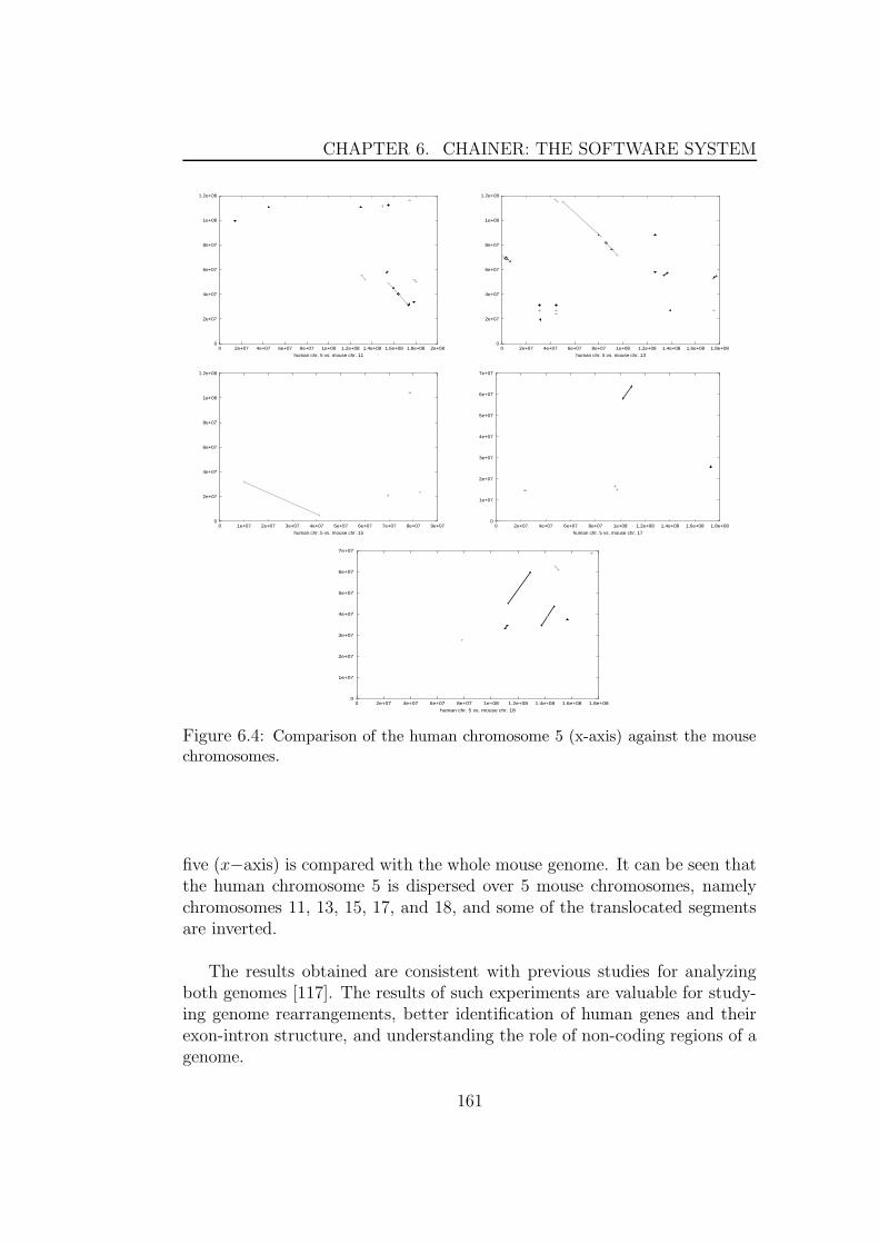
CHAPTER 6. CHAINER: THE SOFTWARE SYSTEM
0
2e+07
4e+07
6e+07
8e+07
1e+08
1.2e+08
0 2e+07 4e+07 6e+07 8e+07 1e+08 1.2e+08 1.4e+08 1.6e+08 1.8e+08 2e+08
human chr. 5 vs. mouse chr. 11
0
2e+07
4e+07
6e+07
8e+07
1e+08
1.2e+08
0 2e+07 4e+07 6e+07 8e+07 1e+08 1.2e+08 1.4e+08 1.6e+08 1.8e+08
human chr. 5 vs. mouse chr. 13
0
2e+07
4e+07
6e+07
8e+07
1e+08
1.2e+08
0 1e+07 2e+07 3e+07 4e+07 5e+07 6e+07 7e+07 8e+07 9e+07
human chr. 5 vs. mouse chr. 15
0
1e+07
2e+07
3e+07
4e+07
5e+07
6e+07
7e+07
0 2e+07 4e+07 6e+07 8e+07 1e+08 1.2e+08 1.4e+08 1.6e+08 1.8e+08
human chr. 5 vs. mouse chr. 17
0
1e+07
2e+07
3e+07
4e+07
5e+07
6e+07
7e+07
0 2e+07 4e+07 6e+07 8e+07 1e+08 1.2e+08 1.4e+08 1.6e+08 1.8e+08
human chr. 5 vs. mouse chr. 18
Figure 6.4: Comparison of the human chromosome 5 (x-axis) against the mousechromosomes.
five (x−axis) is compared with the whole mouse genome. It can be seen thatthe human chromosome 5 is dispersed over 5 mouse chromosomes, namelychromosomes 11, 13, 15, 17, and 18, and some of the translocated segmentsare inverted.
The results obtained are consistent with previous studies for analyzingboth genomes [117]. The results of such experiments are valuable for study-ing genome rearrangements, better identification of human genes and theirexon-intron structure, and understanding the role of non-coding regions of agenome.
161
CHAPTER 6. CHAINER: THE SOFTWARE SYSTEM
6.3 Multiple global alignment
In this section, we demonstrate how our system was used to compare four bac-terial genomes and find homologous regions occurring in all of them. As anexample, we used the four strains of the bacteria Staphylococcus (NC 002745,NC 002758, NC 003923, and NCTC8325). The fragments used were of thetype multiMEMs of minimum length 50 bp. The comparison was done intwo steps. First, CHAINER was called to compute significant local chainsfrom the fragments. In Figure 6.5 (right), we show a projection of the re-sulting chains w.r.t. the first and second genomes. From the figure, we caneasily observe that the four genomes are highly conserved, and the commonsegments of the four genomes are syntenic. Moreover, the common repeatedsequences appear as a grid-like structure on the plot. Accordingly, a moreaccurate comparison can be done by multiple global sequence alignment ofthese genomes. CHAINER was then called again to compute a global chain.Figure 6.5 (left) shows the projection of this global chain w.r.t. the first andsecond genome of the four aforementioned bacterial genomes.
This algorithm is currently used in the multiple global alignment toolMGA [68]. As post-processing of the generated chains, MGA computes adetailed alignment on the character level using the program CLUSTALW.
6.4 Comparing draft genomes
In contrast to a finished genome, a draft genome consists of a set of contigsof unknown order and orientation (a contig is a contiguous tract of knownsubsequence of the genome). Because the cost of finishing a genome can dras-tically exceed the cost of the draft, we anticipate massive amounts of draftmicrobial genomes in the near future. To cope with this data, CHAINERallows to compare a set of draft (or finished) genomes among themselves (afinished genome is considered as a draft genome consisting of a single contig).In the direct mode, CHAINER applies an all-against-all comparison strategy:It searches for local chains (regions of high similarity) between each contig(and its reverse complement, respectively) of a draft genome and all con-tigs of the remaining draft genomes. In the high-throughput mode, however,all draft genomes are compared to each other in a single run of the chain-ing program. To this end, all contigs (and their reverse complements) of adraft genome are concatenated, but a unique separator symbol is insertedbetween consecutive contigs to represent their border. The fragments arethen generated w.r.t. the concatenated sequences and sorted according totheir order in one of the concatenated sequences. This enables us to use the
162
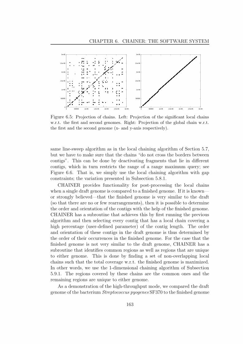
CHAPTER 6. CHAINER: THE SOFTWARE SYSTEM
0
500000
1e+06
1.5e+06
2e+06
2.5e+06
3e+06
0 500000 1e+06 1.5e+06 2e+06 2.5e+06 3e+06 0
500000
1e+06
1.5e+06
2e+06
2.5e+06
3e+06
0 500000 1e+06 1.5e+06 2e+06 2.5e+06 3e+06
Figure 6.5: Projection of chains. Left: Projection of the significant local chainsw.r.t. the first and second genomes. Right: Projection of the global chain w.r.t.the first and the second genome (x- and y-axis respectively).
same line-sweep algorithm as in the local chaining algorithm of Section 5.7,but we have to make sure that the chains “do not cross the borders betweencontigs”. This can be done by deactivating fragments that lie in differentcontigs, which in turn restricts the range of a range maximum query; seeFigure 6.6. That is, we simply use the local chaining algorithm with gapconstraints; the variation presented in Subsection 5.8.1.
CHAINER provides functionality for post-processing the local chainswhen a single draft genome is compared to a finished genome. If it is known—or strongly believed—that the finished genome is very similar to the draft(so that there are no or few rearrangements), then it is possible to determinethe order and orientation of the contigs with the help of the finished genome.CHAINER has a subroutine that achieves this by first running the previousalgorithm and then selecting every contig that has a local chain covering ahigh percentage (user-defined parameter) of the contig length. The orderand orientation of these contigs in the draft genome is thus determined bythe order of their occurrences in the finished genome. For the case that thefinished genome is not very similar to the draft genome, CHAINER has asubroutine that identifies common regions as well as regions that are uniqueto either genome. This is done by finding a set of non-overlapping localchains such that the total coverage w.r.t. the finished genome is maximized.In other words, we use the 1-dimensional chaining algorithm of Subsection5.9.1. The regions covered by these chains are the common ones and theremaining regions are unique to either genome.
As a demonstration of the high-throughput mode, we compared the draftgenome of the bacterium Streptococcus pyogenes SF370 to the finished genome
163
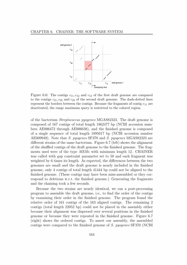
CHAPTER 6. CHAINER: THE SOFTWARE SYSTEM
draft genome 1
draft genome 2
sweeping line
c21
c22
c23
c11
c12
c13
Figure 6.6: The contigs c11, c12 and c13 of the first draft genome are comparedto the contigs c21, c22 and c23 of the second draft genome. The dash-dotted linesrepresent the borders between the contigs. Because the fragments of contig c11 aredeactivated, the range maximum query is restricted to the colored region.
of the bacterium Streptococcus pyogenes MGAS82323. The draft genome iscomposed of 167 contigs of total length 1862477 bp (NCBI accession num-bers AE006472 through AE006638), and the finished genome is composedof a single sequence of total length 1895017 bp (NCBI accession numberAE009949). Note that S. pyogenes SF370 and S. pyogenes MGAS82323 aredifferent strains of the same bacterium. Figure 6.7 (left) shows the alignmentof the shuffled contigs of the draft genome to the finished genome. The frag-ments used were of the type MEMs with minimum length 12. CHAINERwas called with gap constraint parameter set to 50 and each fragment wasweighted by 6 times its length. As expected, the differences between the twogenomes are small and the draft genome is nearly included in the finishedgenome, only 4 contigs of total length 41444 bp could not be aligned to thefinished genome. (These contigs may have been miss-assembled or they cor-respond to deletions w.r.t. the finished genome.) Generating the fragmentsand the chaining took a few seconds.
Because the two strains are nearly identical, we ran a post-processingprogram to assemble the draft genome, i.e., to find the order of the contigsby examining their order in the finished genome. The program found therelative order of 161 contigs of the 163 aligned contigs. The remaining 2contigs (total length 22052 bp) could not be placed in the assembly eitherbecause their alignment was dispersed over several positions in the finishedgenome or because they were repeated in the finished genome. Figure 6.7(right) shows the ordered contigs. To assert our assembly, the assembledcontigs were compared to the finished genome of S. pyogenes SF370 (NCBI
164
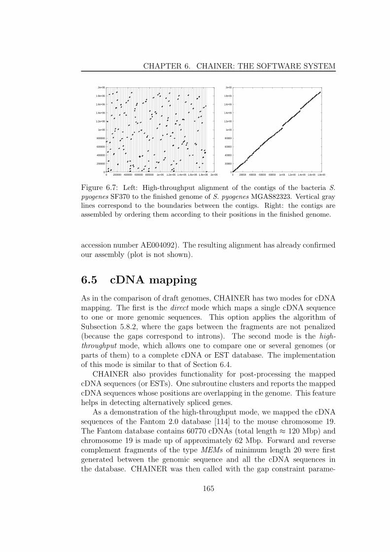
CHAPTER 6. CHAINER: THE SOFTWARE SYSTEM
0
200000
400000
600000
800000
1e+06
1.2e+06
1.4e+06
1.6e+06
1.8e+06
2e+06
0 200000 400000 600000 800000 1e+06 1.2e+06 1.4e+06 1.6e+06 1.8e+06 2e+060
200000
400000
600000
800000
1e+06
1.2e+06
1.4e+06
1.6e+06
1.8e+06
2e+06
0 200000 400000 600000 800000 1e+06 1.2e+06 1.4e+06 1.6e+06 1.8e+06
Figure 6.7: Left: High-throughput alignment of the contigs of the bacteria S.
pyogenes SF370 to the finished genome of S. pyogenes MGAS82323. Vertical graylines correspond to the boundaries between the contigs. Right: the contigs areassembled by ordering them according to their positions in the finished genome.
accession number AE004092). The resulting alignment has already confirmedour assembly (plot is not shown).
6.5 cDNA mapping
As in the comparison of draft genomes, CHAINER has two modes for cDNAmapping. The first is the direct mode which maps a single cDNA sequenceto one or more genomic sequences. This option applies the algorithm ofSubsection 5.8.2, where the gaps between the fragments are not penalized(because the gaps correspond to introns). The second mode is the high-throughput mode, which allows one to compare one or several genomes (orparts of them) to a complete cDNA or EST database. The implementationof this mode is similar to that of Section 6.4.
CHAINER also provides functionality for post-processing the mappedcDNA sequences (or ESTs). One subroutine clusters and reports the mappedcDNA sequences whose positions are overlapping in the genome. This featurehelps in detecting alternatively spliced genes.
As a demonstration of the high-throughput mode, we mapped the cDNAsequences of the Fantom 2.0 database [114] to the mouse chromosome 19.The Fantom database contains 60770 cDNAs (total length ≈ 120 Mbp) andchromosome 19 is made up of approximately 62 Mbp. Forward and reversecomplement fragments of the type MEMs of minimum length 20 were firstgenerated between the genomic sequence and all the cDNA sequences inthe database. CHAINER was then called with the gap constraint parame-
165
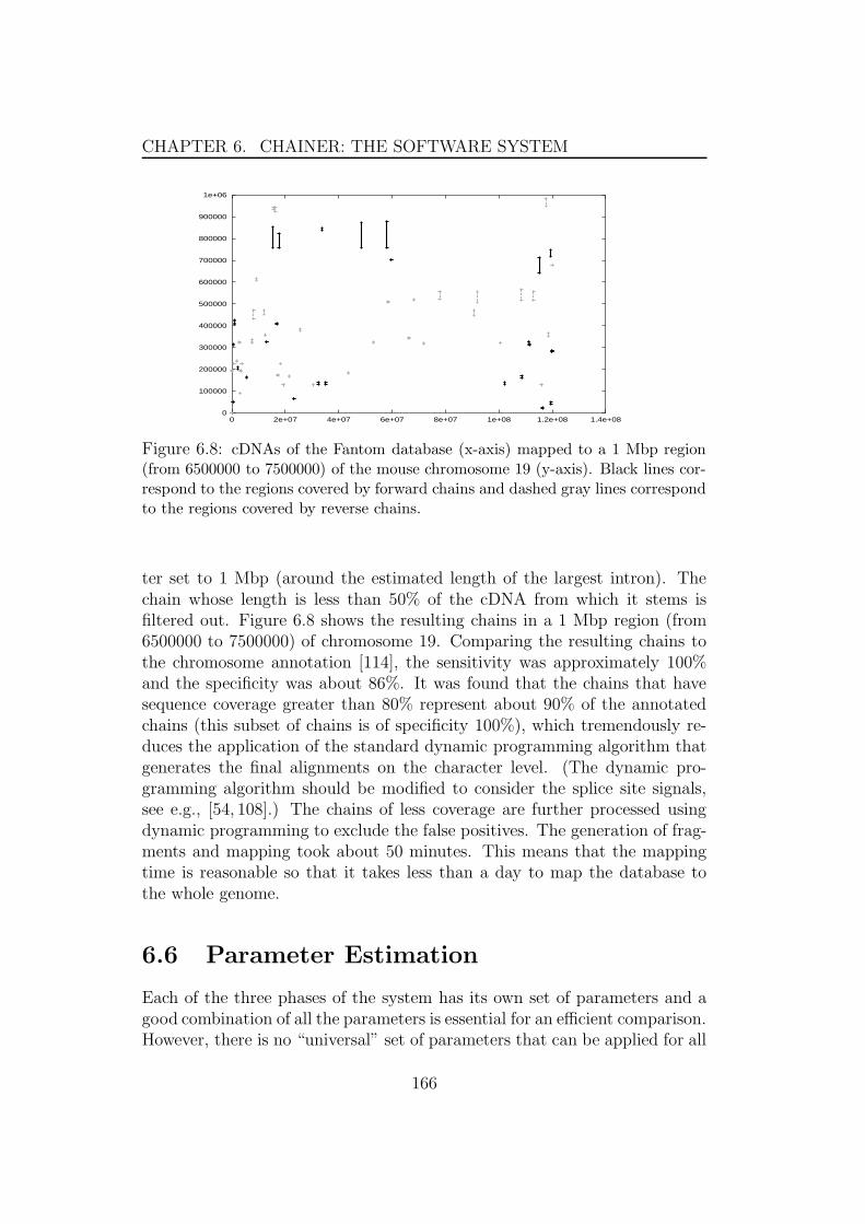
CHAPTER 6. CHAINER: THE SOFTWARE SYSTEM
0
100000
200000
300000
400000
500000
600000
700000
800000
900000
1e+06
0 2e+07 4e+07 6e+07 8e+07 1e+08 1.2e+08 1.4e+08
Figure 6.8: cDNAs of the Fantom database (x-axis) mapped to a 1 Mbp region(from 6500000 to 7500000) of the mouse chromosome 19 (y-axis). Black lines cor-respond to the regions covered by forward chains and dashed gray lines correspondto the regions covered by reverse chains.
ter set to 1 Mbp (around the estimated length of the largest intron). Thechain whose length is less than 50% of the cDNA from which it stems isfiltered out. Figure 6.8 shows the resulting chains in a 1 Mbp region (from6500000 to 7500000) of chromosome 19. Comparing the resulting chains tothe chromosome annotation [114], the sensitivity was approximately 100%and the specificity was about 86%. It was found that the chains that havesequence coverage greater than 80% represent about 90% of the annotatedchains (this subset of chains is of specificity 100%), which tremendously re-duces the application of the standard dynamic programming algorithm thatgenerates the final alignments on the character level. (The dynamic pro-gramming algorithm should be modified to consider the splice site signals,see e.g., [54, 108].) The chains of less coverage are further processed usingdynamic programming to exclude the false positives. The generation of frag-ments and mapping took about 50 minutes. This means that the mappingtime is reasonable so that it takes less than a day to map the database tothe whole genome.
6.6 Parameter Estimation
Each of the three phases of the system has its own set of parameters and agood combination of all the parameters is essential for an efficient comparison.However, there is no “universal” set of parameters that can be applied for all
166
CHAPTER 6. CHAINER: THE SOFTWARE SYSTEM
tasks, i.e., the choice of of parameters will be dependent on the comparativegenomic tasks to be performed.
6.6.1 Parameters for comparing genomes
For the first phase, we have to decide which kind of fragments to use. InChapter 3, we discussed the advantages and disadvantages of different kindsof fragments. There, we reached the conclusion that MEMs or multiMEMsare the most suitable kind of fragments. For either MEMs or multiMEMs, wehave to decide which minimal length to choose. The choice of this minimallength is of extreme importance, as it can affect the efficiency of the threephases. More precisely, if a large minimum fragment length was selected, thenthe number of fragments might be not large enough to cover the all regionsof homology. This can increase the effort exerted in the third phase, which isnot only a refining step, but also a step that compensates deficiencies of thefirst two phases. That is, the whole procedure becomes slow. On the otherhand, if a short minimum fragment length was chosen, then many fragmentscould appear by chance, and their number might be as large as the productof the sequence lengths. This causes a slow chaining phase and accordinglyincreases the whole comparison time. To sum up, a rational choice of thefragment length is a pre-requisite for a good comparison.
There are three methods to determine the suitable minimum fragmentlength. The first method is based on a pre-knowledge of the comparedgenomes. In other words, it assumes that the user has already comparedsub-sequences or genes of these genomes and has been able to identify theminimum match length. The second method uses recursive applications ofthe first and second phases, before moving to the third phase. In theserepeated calls, one starts with a long minimum fragment length and sub-sequently reduces it until the homologous regions are well covered by thefragments. The third method includes the usage of statistical methods toestimate a primary minimum fragment length. This method is used if theuser has no idea about the new dataset; the default parameters of CHAINERwere selected by this method.
To estimate the minimum fragment length based on statistical analy-sis, we use the count statistics as described in [76]. In the count statistics,one counts the number of matches of minimum length ` that can appear bychance. Let Z? denote the number of maximal exact matches of k sequences,where each match has minimum length ` and each of the sequences has aver-age length n. It was shown in [76] that Z? has a limiting Poisson distributionand a statistically significant count would be a number in the tail of the dis-tribution (corresponding to probability < 0.01). In other words, we try to
167
CHAPTER 6. CHAINER: THE SOFTWARE SYSTEM
find, for certain n and k, the minimum match length ` such that its countin the sequences has probability < 0.01. That is, it is unlikely to appear bychance. Table 6.1 (left) shows the recommended minimum fragment lengthsfor different average genome lengths and different number of genomes.
This statistical model, unfortunately, does not take the phylogenetic dis-tance between the organisms into account. If one compares closely relatedorganisms, then they are expected to have large similar regions. In this case,it is preferable to use a longer minimum fragment length. Vice versa, if onecompares distantly related organisms, a shorter fragment length has to bechosen. We tested various genomic sequences at different evolutionary dis-tances, and recommended parameter values; these values are available in theprogram manual.
In the chaining phase, we have to select how the fragments are weighted.The user has the freedom to choose any kind of weighting scheme, but wewould like to draw attention to the following. Fragments are nothing but aseries of matched characters. For producing alignments, the linear scoringscheme, where the weight of a match is a linear function of its length, is themost accepted weighting scheme; see for example [12, 13, 81, 124]. Therefore,CHAINER uses this weighting scheme in the default setting. In fact, theoptimal choice of a weighting scheme for sequence alignment is still highlydebated. In our opinion, the weighting scheme should depend on the analyzeddataset and the comparison task at hand. For example, if one is interestedin aligning regions containing genes to determine gene structures, then thepotential exons can be weighted higher than other non-potential sequences;see for example [16]. (To optimize the scoring scheme for sequence alignmentor any other task is, however, beyond the scope of this thesis.)
The gap constraint parameter can be estimated for regions of high sim-ilarity as follows. Assume that the sequences S1, . . . , Sk , each of aver-age length n, are given. The probability that no match of length at least`, appears is 1 − p`
m, where pm is the probability of a character match ina homologous region. The probability to see no match at all in a regionS1[i1..i1 + W − 1]× · · · × Sk[ik..ik + W − 1], 0 < ij ≤ n, 1 < j < k, of length
W is the joint probability F = (1 − p`m)(W k); this is because the match can
appear at any position in the region W in any of the compared k sequences.We can also count the regions (gaps) of length W in the given sequences.The count is a number as high as O(nkF ). By taking F in the order of 1
nk ,we can estimate the length W for a minimum fragment length `. That is,gaps larger than W are unexpected in a homologous region. Therefore, wetake the estimated W as the default gap constraint in our system. Table 6.1(right) shows the values of W for different values of n, `, and k, and pm = 0.8.
168

CHAPTER 6. CHAINER: THE SOFTWARE SYSTEM
n 2 3 4104..105 15..16 10..12 9..10
105...2×105 17..18 13 112×105...5×105 18..19 14 125×105...106 19..20 15 12..13106 . . . 107 20..25 15..17 14..15107 . . . 108 25..28 18..19 16..17108 . . . 109 29..30 20..23 18..20
n 2 3 4104..105 25..31 7..8 5
105...2×105 32..36 9 52×105...5×105 37..42 10 65×105...106 43..49 11 6106 . . . 107 50..92 12..14 7107 . . . 108 93..172 15..17 8108 . . . 109 173..183 18..24 9
Table 6.1: The left table contains the recommended values of the minimum frag-
ment length ` for different values of n and k. The right table contains the estimated
gap constraint W for different n and k. (The fragment length `, which is used in
estimating W , is obtained by looking up in the left table using n and k.) For
example, for n ∈ [106..107] and k = 2, ` ∈ [20..25]. Hence, W ∈ [50..92].
Again, this statistical model does not consider the phylogenetic distancebetween the organisms. For example, if one compares distantly related or-ganisms, the gap constraint parameter should be set higher. Furthermore, ifthe target of the comparison is to find large conserved segments, where largeindels may occur, gap constraints should be relaxed and set to be as high asthe expected length of the longest deleted segments.
6.6.2 Parameters for cDNA/EST mapping
The minimum fragment length is selected according to the expected min-imum exon length and the quality of the data. (The quality of the datacan be figured out by examining the quality control procedures applied bythe database construction team.) If good quality data is expected, wherethere are a few sequencing errors, then the minimum fragment length canbe selected as high as half of the minimum exon length, otherwise a lowerminimum fragment length has to be used. The gap constraint option is usedto avoid connecting random fragments and to correctly assemble the gene,as discussed in Subsection 5.8.2. The length of the allowed gap is selectedaccording to the maximum intron length expected for the genome at hand.
6.7 Conclusions
In this chapter, we have shown how our algorithms can be integrated ina single software system. We have demonstrated how the system is usedfor performing various comparative genomics tasks, by varying the chaining
169
CHAPTER 6. CHAINER: THE SOFTWARE SYSTEM
phase. We have also proven, by comparing the human and mouse genomes,that our system is able to compare large genomic sequences.
The program MGA, the precursor of our work, has been compared toother software tools performing global alignments [46, 68]. These comparisonshave shown that the quality of MGA was comparable to other software tools,and it runs faster than them (if the same kind of fragments is used). We havefurther improved the running time of the chaining phase of the programMGA; the graph based quadratic time algorithm has been replaced withour subquadratic chaining algorithms. To take one example, chaining about59,000 fragments (multiMEMs of minimum length 20) of three S. aureusgenomes (NC 002745, NC 002758, and NC 003923) takes about 3 minutesusing the graph based approach. This task takes just about 2 seconds usingour chaining algorithms.
Our local chaining algorithm is a novel one. We have verified our resultsby means of comparisons to well-known biological examples. Nevertheless,a rough comparison to the program BLASTZ [124] shows the advantage ofusing our approach. While BLASTZ took about 481 days of CPU time tocompare the human and mouse genomes, our module took just a few days.
Comparing draft genomes became an urgent task, since the cost of fin-ishing genomes has considerably increased. Our module of comparing draftgenomes is still in its primary phase of development. Further improvementsare ongoing.
Our algorithm for cDNA/EST mapping achieves a good compromise be-tween the running time and sensitivity. Our algorithms make it possibleto compare complete databases to complete genomes in a few hours. Totake one example, while the program BLAT (a fast BLAST-like program forcDNA/EST mapping) took about 5 hours to map the Fantom database tochromosome 19, using the default parameters, our module took just about40 minutes.
In this chapter, we approached the problem of estimating certain param-eters, such as the scoring of matches and gap constraints. We used randommodels ignoring the phylogenetic distance between the compared genomes.However, it remains as an open problem to integrate the phylogenetic dis-tance between the organisms in developing such models.
We have visualized the results of our comparisons using dot plots. Ingeneral, developing better visualization and graphical user interface modulesfor large biological data is still an unsolved problem in the field. For ourtasks, we are further faced with the problem of visualizing data in higherdimensions, as a result of comparing multiple genomes. Clearly, novel ideasare demanded to provide an efficient solution to this problem.
170

Chapter 7
Conclusions
In this thesis, we have addressed the problem of large scale analysis and com-parison of genomic sequences. We have started our thesis by introducing thebasic biological concepts that are necessary to understand the problem andour algorithms. Then we have introduced in Chapter 3 a survey of the currentsoftware tools that are able to compare genomic sequences. In this survey, wehave also reviewed and classified the tools according to the underlying com-putational techniques. An interesting observation was that although eachtool has been designed to handle a specific task, most of the tools alreadyshare the same computational strategy. However, the implementation detailsare influenced by the application at hand. From this survey, it is obvious thatthe anchor based strategy became the strategy of choice for most of the soft-ware tools. This is attributed to (1) its subquadratic running time, which isa crucial requirement for the analysis of large genomic sequences, and (2) toits ability to detect short homologies and to accommodate large gaps, i.e.,it adapts to the consequences of the large scale insertions, deletions, andrearrangements of genomic segments.
In Chapter 3, we have also addressed certain aspects that are critical foran efficient comparison of two or multiple genomes. The first of these aspectswas the choice of fragments to be used within the anchor based strategy. Wehave noticed that every tool uses a certain kind of fragments, and the choiceof fragments was made according to the comparative genomic task, the easeof implementation, or due to the lack of an efficient data structure at thattime to generate other kinds of fragments. Therefore, we have discussedthe advantages and disadvantages of using each kind of fragments, and wehave reached the conclusion that the usage of maximal exact matches MEMsachieves a good compromise between the sensitivity and the running timeof the whole comparison procedure. Moreover, the MEMs can be readilyextended to the maximal multiple exact matches multiMEMs in case of com-
171

CHAPTER 7. CONCLUSIONS
paring multiple genomes.The second aspect we have addressed was the choice of the parameters in
the anchor based strategy. The parameters of the surveyed software tools areset according to the authors experience, because there is so far no standardtest dataset.
The final aspect addressed in this survey was the selection of the multiplegenome alignment method. We have shown that there are two methods. Thefirst performs all pairwise comparisons and merges the results into a singlealignment. The second constructs the alignment based on anchors that occursimultaneously in the given genomes. The first method has the advantage ofdetecting similarity between a subset of the compared genomes. However, theproblem of merging the alignments (known as aligning alignments) was shownto be NP-complete [78, 79], and the software tools consequently use heuristicmethods. The second method has higher specificity of finding regions thatare common in all genomes, and it is solvable in polynomial time. However,it misses regions shared by only subsets of the genomes. Perhaps a hybridmethod of both techniques captures the advantages of both procedures.
Regarding the computational methods, most of the tools use simple hash-ing techniques for generating fragments of the type k-mers. This is becauseof the ease of implementation and the reduced space consumption of thehash table. Few of the tools have used the more advanced data structure“suffix tree”, but the large space consumption of the suffix tree (20 bytes percharacter) has limited its use to small and moderate size genomes. As forthe anchoring phase, there are many ad-hoc procedures used in the softwaretools. This is probably because of the lack of algorithms, at that time, thatwere (1) capable of efficiently handling large number of fragments of varioustypes, and (2) flexible enough to solve different comparative genomic tasks.(Recall that fragment generation and determining the anchors are the firsttwo phases of the anchor based strategy.) Chapters 4 and 5 of the thesis havetackled these computational problems.
In Chapter 4, we have introduced the enhanced suffix array, which is anefficient data structure for analyzing large genomic sequences and generatingdifferent kinds of fragments. The principal motivation behind the develop-ment of this data structure was to support the same functionalities as thesuffix tree with less space. We have shown that the enhanced suffix arrayrequires, depending on the task, 5 to 7 bytes per character, which is a greatreduction compared to the suffix tree.
In general, we have shown how every algorithm using the suffix tree canbe systematically replaced by an equivalent one using the enhanced suffixarray. In particular, we have explained in detail how to efficiently computefragments of the types MUMs, multiMUMs, MEMs, and multiMEMs. The
172

CHAPTER 7. CONCLUSIONS
time complexity of these procedures is O(n1 + ..+nk + z), where k ≥ 2 is thenumber of the genomes and z is the number of fragments. Furthermore, wehave explained how the enhanced suffix array can be used for some other ap-plications, such as finding different kinds of repeats (used in studying singlegenomic sequences and data mining), computing Ziv-Lempel decomposition(used in text compression), and computing unique substrings (used in thedesign of oligonucleotides). Our experimental results have shown that theenhanced suffix array algorithms are many times faster than the correspond-ing ones based on the suffix tree.
In the epilogue of Chapter 4, we have mentioned some of the open prob-lems. The most notable one, which we expect to be solved in the near future,is the generation of multiMEMs by constructing the enhanced suffix arrayof only one sequence and matching the other sequences against it. (We haveshown in the chapter how to generate multiMEMs using the enhanced suffixarray of the string made up of the concatenated sequences.) Furthermore, theincorporation of the rare and infrequent multiMEMs, which allow us to gen-erate multiMEMs such that their number does not grow exponentially withthe number of the given genomes, is a significant variation of this problem.
In Chapter 5, we have presented our chaining algorithms. For comparingclosely related genomes, where the homologous regions are conserved in order,global chaining is the procedure of choice. For comparing distantly relatedgenomes, where rearrangement events are expected, the local chaining is theprocedure of choice. Given a set of m fragments, our algorithms computeoptimal global and local chains in subquadratic time and linear space: Fork = 2 genomes, our algorithms take
• O(m log log m) time and O(m) space without gap costs,
• O(m log log m) time and O(m) space for gap costs in the L1 metric,
• O(m log m log log m) time and O(m) space for the sum-of-pairs gap costand for gap costs in the L∞ metric.
If the start and end points of the fragments are not sorted w.r.t. one dimen-sion, then the complexity is dominated, in case of neglecting gap costs andgap costs in the L1 metric, by the sorting procedure, which takes O(m logm).
For k > 2 genomes, our algorithms that are based on the semi-dynamicrange tree take
• O(m logk−2 m log log m) time and O(m logk−2 m) space without gapcosts,
• O(m logk−2 m log log m) time and O(m logk−2 m) space for gap costs inthe L1 metric,
173
CHAPTER 7. CONCLUSIONS
• O(k! m logk−1 m log log m) time and O(k! m logk−1 m) space for thesum-of-pairs gap cost and for gap costs in the L∞ metric.
These results improve upon previous results obtained by Myers and Miller[111]. More precisely, for gap costs in the L1-metric we reduced the spacecomplexity by a log-factor and improved the time complexity by a factorlog2 m
log log m. For the sum-of-pairs gap cost, we improved the time complexity by
a factor log m
log log m.
The above mentioned results assume that the range tree is the basic datastructure that manipulates the points. In fact, our algorithms can employ anyother data structure that supports range search for maximum. Therefore, wehave investigated the usage of the kd -tree and we introduced the first timeanalysis for the chaining algorithms based on this data structure: They take
O((k − 1)m2− 1k−1 ) time and O(m) space for gap costs in the L1 metric, and
O((k!)m2− 1k ) time and O(k!m) space for the sum-of-pairs gap costs. Our
experimental results have shown that the kd -tree is superior to the rangetree in practice. Hence, we decided to implement our algorithms based onkd -trees.
In Chapter 5, we have also introduced two basic variations of the chainingalgorithms: chaining with gap constraints and cDNA/EST mapping. Thesevariations also take subquadratic time and require linear space.
In the conclusions of that chapter, we have discussed the challenge ofonline chaining, namely the application of an efficient dynamic data structurethat supports range maximum queries. The current dynamic data structuresare very complicated and their running time is higher than that of the semi-dynamic ones.
Finally, in Chapter 6, we have introduced our software system CHAINERthat implements and integrates the algorithms presented in this thesis. Wehave demonstrated how CHAINER is used to globally align multiple genomes,to detect translocation events, and to detect genome inversions. We havecompared our results to known biological examples and the results we haveobtained were consistent with known results.
We have also shown how our system can be used to compare draft genomesand how it can help to assemble them. Our post-processing module for as-sembling these contigs assumes that the draft and the finished genomes arevery closely related so that no rearrangement and segmental duplicationsexist. Extending this module to handle less related genomes, where rear-rangements and duplications are expected, forms an obvious direction forfuture work.
As a final comparative genomic task, we have shown how our systemcan be used to map a cDNA/EST database to a genomic sequence. We
174

CHAPTER 7. CONCLUSIONS
have evaluated our results by comparing our mapping to well annotated se-quences. The accuracy of our mapping was so good that we were encouragedto add further functionalities, such as the clustering of cDNA/ESTs to detectalternative splice variants.
At the end of Chapter 6, we have shown how the default parameters ofthe system can be estimated. We have used a statistical model based on thecount statistics of random matches. A future task is to optimize this modelby taking the evolutionary distances between the compared sequences intoaccount.
Lastly, but not least, we think that our algorithms and the softwaresystem presented within this thesis will enable researchers to perform highthroughput experiments, even with limited computational resources. We ex-pect that our system will help to address, on a global scale, questions suchas the role of non-coding regions and repeated sequences in a genome. More-over, we believe that it will help to achieve a lot of progress in solving theproblems of elucidating genome evolution, and the exact identification ofgene structure.
175

Bibliography
[1] M. I. Abouelhoda, S. Kurtz, and E. Ohlebusch. The enhanced suffixarray and its applications to genome analysis. In Proceedings of the2nd Workshop on Algorithms in Bioinformatics, volume 2452 of LNCS,pages 449–463. Springer-Verlag, 2002.
[2] M. I. Abouelhoda, S. Kurtz, and E. Ohlebusch. Replacing suffix treeswith enhanced suffix arrays. Journal of Discrete Algorithms, 2(1):53–86, 2004.
[3] M. I. Abouelhoda and E. Ohlebusch. A local chaining algorithm and itsapplications in comparative genomics. In Proceedings of the 3rd Work-shop on Algorithms in Bioinformatics, volume 2812 of LNBI, pages1–16. Springer Verlag, 2003.
[4] M. I. Abouelhoda and E. Ohlebusch. Multiple genome alignment:Chaining algorithms revisited. In Proceedings of the 14th Annual Sym-posium on Combinatorial Pattern Matching, LNCS, volume 2676 ofLNCS, pages 1–16. Springer Verlag, 2003.
[5] M. I. Abouelhoda and E. Ohlebusch. CHAINER: Software for compar-ing genomes. In Proceedings of the 12th International Conference onIntelligent Systems for Molecular Biology/3rd European Conference onComputational Biology, 2004.
[6] M. I. Abouelhoda and E. Ohlebusch. Chaining algorithms and appli-cations in comparative genomics. Journal of Discrete Algorithms, inpress.
[7] M.I. Abouelhoda, S. Kurtz, and E. Ohlebusch. The enhanced suffixarrays. In Handbook of Computational Molecular Biology. CRC Press,in press.
[8] M.I. Abouelhoda, E. Ohlebusch, and S. Kurtz. Optimal Exact StringMatching Based on Suffix Arrays. In Proceedings of the 9th Inter-
177

BIBLIOGRAPHY
national Symposium on String Processing and Information Retrieval,volume 2476 of LNCS, pages 31–43. Springer-Verlag, 2002.
[9] P. Agarwal. Range searching. In Handbook of Discrete and Computa-tional Geometry, chapter 31, pages 575–603. CRC Press LLC, 1997.
[10] A. Aho and M. Corasick. Efficient string matching: An aid to biblio-graphic search. Communications of the ACM, 18:333–340, 1975.
[11] T. Albert. Molecular Biology. W. H. Freeman and Company, NewYork, 2002.
[12] S. F. Altschul, W. Gish, W. Miller, E. W. Myers, and D. J. Lipman.A basic local alignment search tool. Journal of Molecular Biology,215:403–410, 1990.
[13] S.F. Altschul, T. L. Madden, A. A. Schaffer, and et al.˙Gapped BLASTand PSI-BLAST: A new generation of protein database search pro-grams. Nucleic Acids Research, 25(17):3389–3402, 1997.
[14] E. L. Anson and E. W. Myers. ReAligner: A program for refiningDNA sequence multi-alignments. Journal of Computational Biology,4(3):369–383, 1997.
[15] A. Apostolico. The myriad virtues of subword trees. In CombinatorialAlgorithms on Words, NATO ISI, pages 85–96. Springer-Verlag, 1985.
[16] V. Bafna and D.H. Huson. The conserved exon method for gene finding.In Proceedings of the 8th Int. Conference on Intelligent Systems forMolecular Biology, pages 3–12. AAAI Press, 2000.
[17] V. Bafna, B. Narayanan, and R. Ravi. Nonoverlapping local align-ments (weighted independent sets of axis-parallel rectangles). DiscreteApplied Mathematics, 71:41–53, 1996.
[18] R. Bar-Yehuda, M.M. Halldorsson, J. Naor, and H. Shachnai. Schedul-ing split intervals. In Proceedings of the 13th ACM-SIAM Symposiumon Discrete Algorithms, pages 732–741, 2002.
[19] S. Batzoglu, L. Pachter, J. P. Mesirov, B. Berger, and E. S. Lander. Hu-man and mouse gene structure: Comparative analysis and applicationto exon prediction. Genome Research, 10:950–958, 2001.
178
BIBLIOGRAPHY
[20] M. Beckstette, D. Strothmann, R. Homann, R. Giegerich, and S. Kurtz.Fast and sensitive matching of position specific scoring matrices usingenhanced suffix arrays. In Proceedings of the German Conference onBioinformatics, pages 53–64. GI, 2004.
[21] M. A. Bender and M. Farach-Colton. The LCA problem revisited. InLatin American Theoretical INformatics, pages 88–94, 2000.
[22] J. L. Bentley. Multidimensional binary search trees in database appli-cations. IEEE Transactions on Software Engineering, SE-5(4):333–340,1979.
[23] J. L. Bentley. Multidimensional binary search trees used for associativesearching. Communications of the ACM, 18(9):509–517, 1979.
[24] J. L. Bentley. Kd-trees for semidynamic point sets. In Proceedings ofthe 6th Annual ACM Symposium on Computational Geometry, pages187–197. ACM, 1990.
[25] J. L. Bentley and J. Saxe. Decomposable searching problems. I: Staticto dynamic transformations. Journal of Algorithms, 1:301–358, 1980.
[26] J. L. Bentley and R. Sedgewick. Fast algorithms for sorting and search-ing strings. In Proceedings of the 8th ACM-SIAM Symposium on Dis-crete Algorithms, pages 360–369, 1997.
[27] A. Bernal, U. Ear, and N. Kyrpide. Genomes OnLine Database(GOLD): A monitor of genome projects world-wide. Nucleic AcidsResearch, 1(29):126–127, 2001.
[28] N. Bray, I. Dubchak, and L. Pachter. AVID: A global alignment pro-gram. Genome Research, 13:97–102, 2003.
[29] N. Bray and L. Pachter. MAVID: Multiple alignment server. NucleicAcids Research, 31:3525–3526, 2003.
[30] T. Brown. The Genome. W. H. Freeman and Company, New York,2002.
[31] M. Brudno, C. B. Do, G. M. Cooper, M. F. Kim, E. D. Davydov,NISC Comparative Sequencing Program, E. D. Green, A. Sidow, andS. Batzoglou. LAGAN and Multi-LAGAN: Efficient tools for large-scalemultiple alignment of genomic DNA. Genome Research, 13(4):721–731,2003.
179

BIBLIOGRAPHY
[32] M. Brudno, S. Malde, A. Poliakov, C. B. Do, O. Couronne, I. Dubchak,and S. Batzoglou. Glocal alignment: Finding rearrangements duringalignment. Bioinformatics, 19:i54–i62, 2003.
[33] M. Brudno and B. Morgenstern. Fast and sensitive alignment of largegenomic sequences. In Proceedings of the IEEE Computer SocietyBioinformatics Conference (CSB’02), pages 138–150. IEEE, 2002.
[34] J. Buhler. Efficient large-scale sequence comparison by locality-sensitive hashing. Bioinformatics, 17(5):419–428, 2001.
[35] M. Burrows and D. J. Wheeler. A block-sorting lossless data compres-sion algorithm. Research Report 124, Digital Systems Research Center,1994.
[36] P. Chain, S. Kurtz, E. Ohlebusch, and T. Slezak. An applications-focused review of comparative genomics tools: Capabilities, limitationsand future challenges. Briefings in Bioinformatics, 4(2):105–123, 2003.
[37] W.I. Chang and E.L. Lawler. Sublinear approximate string matchingand biological applications. Algorithmica, 12(4/5):327–344, 1994.
[38] K.-M. Chao and W. Miller. Linear-space algorithms that build localalignments from fragments. Algorithmica, 13:106–134, 1995.
[39] Y. Chiang and R. Tamassia. Dynamic algorithms in computationalgeometry. Technical report, Brown University, 1992.
[40] T. H. Cormen, C. E. Leiserson, and R. L. Rivest. Introduction toAlgorithms. MIT Press, Cambridge, MA, 1990.
[41] W. Cunto, G. Lau, and P. Flajolet. Analysis of Kdt-trees: Kd-treesimproved by local reorganisations. In Proceedings of the 1st Workshopon Algorithms and Data Structures, volume 382 of LNCS, pages 24–38.Springer-Verlag, 1989.
[42] I. Dagan, M. C. Golumbic, and R. Y. Pinter. Trapezoid graphs andtheir coloring. Discrete Applied Mathematics, 21:35–46, 1988.
[43] A. C. E. Darling, B. Mau, F. R. Blattner, and N. T. Perna. MAUVE:Multiple alignment of conserved genomic sequence with rearrange-ments. Genome Research, 14:1394–1403, 2004.
180
BIBLIOGRAPHY
[44] A. L. Delcher, S. Kasif, R. D. Fleischmann, J. Peterson, O. White, andS. L. Salzberg. Alignment of whole genomes. Nucleic Acids Research,27(11):2369–2376, 1999.
[45] A. L. Delcher, A. Phillippy, J. Carlton, and S. L. Salzberg. Fast al-gorithms for large-scale genome alignment and comparison. NucleicAcids Research, 30(11):2478–2483, 2002.
[46] J. S. Deogen, J. Yang, and F. Ma. EMAGEN: An efficient approachto multiple genome alignment. In Proceedings of the 2nd Asia PacificBioinformatics Conference (APBC2004), pages 113–122, 2004.
[47] R. Dietz and R. Raman. Persistence, amortization and randomization.In Proceedings of the 2nd annual symposium ACM-SIAM Symposiumon Discrete Algorithms, pages 78–88, 1991.
[48] J. A. Eisen, J. F. Heidelberg, O. White, and S. L. Salzberg. Evidencefor symmetric chromosomal inversions around the replication origin inbacteria. Genome Biology, 1(6):1–9, 2000.
[49] S. J. Emrich, M. Lowe, and A. L. Delcher. PROBEmer: A web-basedsoftware tool for selecting optimal DNA oligos. Nucleic Acids Research,31(13):3746–3750, 2003.
[50] D. Eppstein, Giancarlo R. Galil, Z., and G. F. Italiano. Sparse dynamicprogramming. I: Linear cost functions; II: Convex and concave costfunctions. Journal of the ACM, 39:519–567, 1992.
[51] S. Felsner, R. Muller, and L. Wernisch. Trapezoid graphs and gen-eralizations, geometry and algorithms. Discrete Applied Mathematics,74(1):13–32, 1997.
[52] P. Ferragina and G. Manzini. Opportunistic data structures with appli-cations. In Proceedings of the 41st Annual Symposium on Foundationsof Computer Science, pages 390–398. IEEE, 2000.
[53] R.D. Fleischmann, M. D. Adams, O. White, R. A. Clayton, E. F. Kirk-ness, A. R. Kerlavage, C. J. Bult, J. F. Tomb, B. A. Dougherty, J. M.Merrick, and et al. Whole-genome random sequencing and assembly ofHaemophilus influenzae Rd. Science, 269(5223):496–512, 1995.
[54] L. Florea, G. Hartzell, Z. Zhang, G. Rubin, and W. Miller. A computerprogram for aligning a cDNA sequence with a genomic DNA sequence.Genome Research, 8:967–974, 1998.
181

BIBLIOGRAPHY
[55] J. H. Friedman, J. L. Bentley, and R. A. Finkel. An algorithm forfinding best matches in logarithmic expected time. ACM Transactionson Mathematical Software, 3(3):209–226, 1997.
[56] Z. Galil and K. Park. Dynamic programming with convexity, concavityand sparsity. Theoretical Computer Science, 92:49–76, 1992.
[57] R. Giegerich and S. Kurtz. From Ukkonen to McCreight and Weiner:A unifying view of linear-time suffix tree construction. Algorithmica,19:331–353, 1997.
[58] A. Goffeau, B. G. Barrell, H. Bussey, R. W. Davis, B. Dujon, H. Feld-mann, F. Galibert, J. D. Hoheisel, C. Jacq, M. Johnston, and et al.˙Life with 6000 genes. Science, 274(5287):546–567, 1996.
[59] G. Gonnet, R. Baeza-Yates, and T. Snider. New indices for text: PATtrees and PAT arrays. In Information Retrieval: Algorithms and DataStructures, pages 66–82. Prentice-Hall, 1992.
[60] R. Grossi and J. S. Vitter. Compressed suffix arrays and suffix treeswith applications to text indexing and string matching. In ACM Sym-posium on the Theory of Computing (STOC 2000), pages 397–406.ACM Press, 2000.
[61] L. J. Guibas and J. Stolfi. On computing all north-east nearest neigh-bors in the L1 metric. Information Processing Letters , 17(4):219–223,1983.
[62] D. Gusfield. Algorithms on Strings, Trees, and Sequences. CambridgeUniversity Press, New York, 1997.
[63] D. Gusfield and J. Stoye. Linear time algorithms for finding and repre-senting all the tandem repeats in a string. Report CSE-98-4, ComputerScience Division, University of California, Davis, 1998.
[64] A. L. Halpern, D. H. Huson, and K. Reinert. Segment match refinementand applications. In Proceedings of the 2nd Workshop on Algorithms inBioinformatics, volume 2452 of LNCS, pages 126–139. Springer Verlag,2002.
[65] R. Himmelreich, H. Hilbert, H. Plagens, E. Pirkl, B. C. Li, and R. Her-rmann. Complete sequence analysis of the genome of the bacteriumMycoplasma pneumoniae. Nucleic Acids Research, 24(22):4420–4449,1996.
182
BIBLIOGRAPHY
[66] R. Himmelreich, H. Plagens, H. Hilbert, B. Reiner, and R. Herrmann.Comparative analysis of the genomes of the bacteria Mycoplasma pneu-moniae and Mycoplasma genitalium. Nucleic Acids Research, 25:701–712, 1997.
[67] D. S. Hirschberg. A linear space algorithm for computing maximalcommon subsequences. Communications of the ACM , 18:341–343,1975.
[68] M. Hohl, S. Kurtz, and E. Ohlebusch. Efficient multiple genome align-ment. Bioinformatics, 18:S312–S320, 2002.
[69] W. K. Hon and K. Sadakane. Space-economical algorithms for findingmaximal unique matches. In Proceedings of the 13th Annual Symposiumon Combinatorial Pattern Matching, volume 2452 of LNCS, pages 144–152. Springer-Verlag, 2002.
[70] X. Huang and W. Miller. A time-efficient, linear space local similarityalgorithm. Advances in Applied Mathematics, 12:337–357, 1991.
[71] D. Hughes. Evaluating genome dynamics: The constraints on rear-rangements within bacterial genomes. Genome Biology, 1(6):1–8, 2000.
[72] International Human Genome Sequencing Consortium. Initial sequenc-ing and analysis of the human genome. Nature, 409:860–921, 2001.
[73] J. B. Jenkins. Human Genetics. Harper & Row, New York, 2nd edition,1990.
[74] D. B. Johnson. A priority queue in which initialization and queueoperations take O(log log D) time. Mathematical Systems Theory,15(4):295–310, 1982.
[75] J. Karkkainen and P. Sanders. Simple linear work suffix array construc-tion. In Proceedings of the 30th International Colloquium on Automata,Languages and Programming, volume 2719 of LNCS, pages 943–955.Springer-Verlag, 2003.
[76] S. Karlin, F. Ost, and B. E. Blaisdell. Patterns in DNA and amino acidsequences and their statistical significance. In Mathematical Methodsfor DNA Sequences, pages 133–157. CRC Press, 1989.
[77] T. Kasai, G. Lee, H. Arimura, S. Arikawa, and K. Park. Linear-timelongest-common-prefix computation in suffix arrays and its applica-tions. In Proceedings of the 12th Annual Symposium on Combinatorial
183

BIBLIOGRAPHY
Pattern Matching, volume 2089 of LNCS, pages 181–192. Springer-Verlag, 2001.
[78] J. Kececioglu. The maximum weight trace problem in multiple se-quence alignment. In Proceedings of the 4th Annual Symposium onCombinatorial Pattern Matching, volume 684 of LNCS, pages 106–119.Springer-Verlag, 1993.
[79] J. Kececioglu and D. Starrett. Aligning alignments exactly. In Pro-ceedings of the 8th Annual International Conference on Research inComputational Molecular Biology, pages 85–96. ACM, 2004.
[80] W. J. Kent, R. Baertsch, A. Hinrichs, W. Miller, and D. Haussler.Evolution’s cauldron: Duplication, deletion, and rearrangement in themouse and human genomes. Proceedings of the National Academy ofScience (PNAS), 100(20):11484–11489, 2003.
[81] W.J. Kent. BLAT—the BLAST-like alignment tool. Genome Research,12:656–664, 2002.
[82] W.J. Kent and A.M. Zahler. Conservation, regulation, synteny, and in-trons in large-scale C. briggsae–C. elegans genomic alignment. GenomeResearch, 10:1115–1125, 2000.
[83] D. K. Kim, J. S. Sim, H. Park, and K. Park. Linear-time construc-tion of suffix arrays. In Proceedings of the 14th Annual Symposium onCombinatorial Pattern Matching, volume 2676 of LNCS, pages 186–199. Springer-Verlag, 2003.
[84] J. Knight, D. Gusfield, and J. Stoye. The Strmat Software-Package,1998. http://www.cs.ucdavis.edu/∼gusfield/strmat.tar.gz.
[85] P. Ko and S. Aluru. Space efficient linear time construction of suffixarrays. In Proceedings of the 14th Annual Symposium on CombinatorialPattern Matching, volume 2676 of LNCS, pages 200–210. Springer-Verlag, 2003.
[86] R. Kolpakov and G. Kucherov. Finding maximal repetitions in a wordin linear time. In Proceedings of the 40th Annual Symposium on Foun-dations of Computer Science, pages 596–604. IEEE, 1999.
[87] M. J. Kreveld and M. H. Overmars. Divided kd -trees. Algorithmica,6(6):840–858, 1991.
184

BIBLIOGRAPHY
[88] J. Kruger, A. Sczyrba, S. Kurtz, and R. Giegerich. e2g: An interactiveweb-based server for efficiently mapping large EST and cDNA sets togenomic sequences. Nucleic Acids Research, 32:W301–W304, 2004.
[89] S. Kurtz. Reducing the space requirement of suffix trees. Software—Practice and Experience, 29(13):1149–1171, 1999.
[90] S. Kurtz. The Vmatch: Large scale sequence analysis software,http://www.vmatch.de.
[91] S. Kurtz, J. V. Choudhuri, E. Ohlebusch, C. Schleiermacher, J. Stoye,and R. Giegerich. REPuter: The manifold applications of repeat anal-ysis on a genomic scale. Nucleic Acids Research, 29(22):4633–4642,2001.
[92] S. Kurtz, A. Phillipy, A. L. Delcher, M. Smoot, M. Shumway, C. An-tonescu, and S. L. Salzberg. Versatile and open software for comparinglarge genomes. Genome Biology, 5(2):R12, 2004.
[93] N. J. Larsson and K. Sadakane. Faster suffix sorting. Technical ReportLU-CS-TR:99-214, Department of Computer Science, Lund University,1999.
[94] E. L. Lawler. Combinatorial Optimization: Networks and Matroids.Holt, Rinehart, and Winston, New York, 1976.
[95] D. T. Lee and C. K. Wong. Worst-case analysis for region and partialregion searches in multidimensional binary search trees and balancedquad trees. Acta Informatica, 9:23–29, 1977.
[96] M. Y. Leung, B. E. Blaisdell, C. Burge, and S. Karlin. An efficientalgorithm for identifying matches with errors in multiple long molecularsequences. Journal of Molecular Biology, 221:1367–1378, 1991.
[97] J. R. Lobry. Asymmetric substitution patterns in the two DNA strandsof bacteria. Molecular Biology and Evolution, 13(5):660–665, 1996.
[98] H Lodish, A. Berk, S. L. Zipursky, P. Matsudaira, D. Baltimore, andJ. Darnell. Molecular Cell Biology. W. H. Freeman and Company, NewYork, 1999.
[99] B. Ma, J. Tromp, and M. Li. PatternHuner: Faster and more sensitivehomology search. Bioinformatics, 18(3):440–445, 2002.
185
BIBLIOGRAPHY
[100] U. Manber and E. W. Myers. Suffix arrays: A new method for on-linestring searches. SIAM Journal on Computing, 22(5):935–948, 1993.
[101] E. M. McCreight. A space-economical suffix tree construction algo-rithm. Journal of Algorithms, 23(2):262–272, 1976.
[102] E. M. McCreight. Priority search trees. SIAM Journal of Computing,14(2):257–276, 1985.
[103] K. Mehlhorn and S. Naher. Bounded ordered dictionaries inO(log log N) time and O(n) space. Information Processing Letters,35(4):183–189, 1990.
[104] K. Mehlhorn and S. Naher. Dynamic fractional cascading. Algorith-mica, 5:215–241, 1990.
[105] W. Miller and E. W. Myers. Sequence comparison with concave weight-ing functions. Bulletin of Mathematical Biology, 50:97–120, 1988.
[106] B. Morgenstern. DIALIGN 2: Improvement of the segment-to-segmentapproach to multiple sequence alignment. Bioinformatics, 15(3):211–218, 1999.
[107] B. Morgenstern. A space efficient algorithm for aligning large genomicsequences. Bioinformatics, 16(10):948–949, 2000.
[108] R. Mott. EST GENOME: A program to align spliced DNA sequencesto unspliced genomic DNA. Computer Applications in the Biosciences(CABIOS), 4:477–478, 1997.
[109] E. W. Myers and X. Huang. An O(n2 log n) restriction map comparisonand search algorithm. Bulletin of Mathematical Biology, 54(4):599–618,1992.
[110] G. Myers and W. Miller. Optimal alignments in linear space. ComputerApplications in the Biosciences (CABIOS), 4:11–17, 1988.
[111] G. Myers and W. Miller. Chaining multiple-alignment fragments insub-quadratic time. Proceedings of the 6th annual ACM-SIAM sympo-sium on Discrete algorithms, pages 38–47, 1995.
[112] S. B. Needleman and C. D. Wunsch. A general method applicable tothe search for similarities in the amino-acid sequence of two proteins.Journal of Molecular Biology, 48:443–453, 1970.
186
BIBLIOGRAPHY
[113] E. Ohlebusch and M. I. Abouelhoda. Chaining algorithms and ap-plications in comparative genomics. In Handbook of ComputationalMolecular Biology. CRC Press, in press.
[114] Y. Okazaki, M. Furuno, T. Kasukawa, J. Adachi, H. Bono, S. Kondo,I. Nikaido, N. Osato, R. Saito, and et. al Suzuki, H. Analysis ofthe mouse transcriptome based on functional annotation of 60770 full-length cDNAs. Nature, 420(6951):563–573, 2002.
[115] Committee on Mapping and Sequencing the Human Genome, NationalResearch Council. Mapping and Sequencing the Human Genome. TheNational Academies Press, Washington, DC, 1988.
[116] W. R. Pearson and D. J. Lipman. Improved tools for biological sequencecomparison. Proceedings of the National Academy of Science (PNAS),85:2444–2448, 1988.
[117] P. Pevzner and G. Tesler. Genome rearrangements in mammaliangenomes: Lessons from human and mouse genomic sequences. GenomeResearch, 13:13–26, 2003.
[118] F. P. Preparata and M. I. Shamos. Computational Geometry: AnIntroduction. Springer-Verlag, New York, 1985.
[119] W. Pugh. Skip lists: A probabilistic alternative to balanced trees.Communications of the ACM , 33:668–676, 1990.
[120] T. D. Read, R. C. Brunham, C. Shen, S. R. Gill, J. F. Heidelberg,O. White, E. K. Hickey, J. Peterson, T. Utterback, K. Berry, and et al.Genome sequences of Chlamydia trachomatis MoPn and Chlamydiapneumoniae AR39. Nucleic Acids Research, 28(6):1397–1406, 2000.
[121] K. Sadakane. Succinct representations of lcp information and improve-ments in the compressed suffix arrays. In Proceedings of the 13th ACM-SIAM Symposium on Discrete Algorithms, pages 225–232, 2002.
[122] H. Samet. The Design and Analysis of Spatial Data Structures.Addison-Wesley, MA, 1990.
[123] S. Schwartz, L. Elnitski, M. Li, M. Weirauch, C. Riemer, A. Smit,NISC Comparative Sequencing Program, E. D. Green, R. C. Hardison,and W. Miller. MultiPipMaker and supporting tools: Alignments andanalysis of multiple genomic DNA sequences. Nucleic Acids Research,31(13):3518–3524, 2003.
187

BIBLIOGRAPHY
[124] S. Schwartz, W. J. Kent, A. Smit, Z. Zhang, R. Baertsch, R. C.Hardison, D. Haussler, and W. Miller. Human-mouse alignments withBLASTZ. Genome Research, 13:103–107, 2003.
[125] S. Schwartz, Z. Zhang, K. A. Frazer, A. Smit, C. Riemer, J. Bouck,R. Gibbs, R. Hardison, and W. Miller. PipMaker–a web server foraligning two genomic DNA sequences. Genome Research, 10(4):577–586, 2000.
[126] A. Smit and P. Green. RepeatMasker, http://www.repeatmasker.org/.
[127] W. Smith and M. S. Waterman. Identification of common molecularsubsequences. Journal of Computational Biology, 147:195–197, 1981.
[128] E. Sobel and M. Martinez. A multiple sequence alignment program.Nucleic Acids Research, 14:363–374, 1986.
[129] R. Sproull. Refinements to nearest neighbor searching in K-dimensionaltrees. Algorithmica, 6:579–589, 1991.
[130] J. Stoye and D. Gusfield. Simple and flexible detection of contiguousrepeats using a suffix tree. Theoretical Computer Science, 270(1-2):843–856, 2002.
[131] J. Thompson, D. Higgins, and Gibson. T. CLUSTALW: Improving thesensitivity of progressive multiple sequence alignment through sequenceweighting, position specific gap penalties, and weight matrix choice.Nucleic Acids Research, 22:4673–4680, 1994.
[132] P. van Emde Boas. Preserving order in a forest in less than logarith-mic time and linear space. Information Processing Letters, 6(3):80–82,1977.
[133] P. van Emde Boas, R. Kaas, and E. Zijlstra. Design and implementationof an efficient priority queue. Mathematical Systems Theory, 10:99–127,1977.
[134] J. S. Varre, J. P. Delahaye, and E. Rivals. Transformation distances:A family of dissimilarity measures based on movements of segments.Bioinformatics, 15(3):194–202, 1999.
[135] J. C. Venter, M. D. Adams, E. W. Myers, P. W. Li, R. J. Mural, G. G.Sutton, H. O. Smith, M. Yandell, C. A. Evans, R. A. Holt, and et al.˙The sequence of the human genome. Science, 291(5507):1304–1351,2001.
188
BIBLIOGRAPHY
[136] P. Vincens, L. Buffat, C. Andre, J. Chevrolat, J. Boisvieux, and S. Ha-zout. A strategy for finding regions of similarity in complete genomesequences. Bioinformatics, 14(8):715–725, 1998.
[137] P. Weiner. Linear pattern matching algorithms. In Proceedings of the14th IEEE Annual Symposium on Switching and Automata Theory,pages 1–11, 1973.
[138] W. J. Wilbur and D. J. Lipman. Rapid similarity searches of nucleicacid and protein data banks. Proceedings of the National Academy ofScience USA, 80:726–730, 1983.
[139] D. E. Willard. New data structures for orthogonal range queries. SIAMJournal of Computing, 14:232–253, 1985.
[140] D. E. Willard and G. S. Lueker. Adding range restriction capability todynamic data structures. Journal of ACM, 32:597–617, 1985.
[141] Z. Zhang, B. Raghavachari, R. C. Hardison, and W. C. Miller. Chainingmultiple-alignment blocks. Journal of Computational Biology, 1:51–64,1994.
[142] J. Ziv and A. Lempel. A universal algorithm for sequential data com-pression. IEEE Transactions on Information Theory, 23(3):337–343,1997.
189
Deutsche Zusammenfassung
Vergleichende Genomanalyse ist ein relativ neues Gebiet der Bioinformatik.Die Kernmethode dieses Gebietes ist der direkte Vergleich des Genoms—des vollstandigen genetischen Materials—eines Organismus mit dem einesanderen Organismus oder mit dem mehrerer anderer Organismen. SolcheAnalysen erlauben die Identifikation von Genen sowie die Vorhersage vonderen Funktionen, das Erkennen von Ahnlichkeit und Verschiedenheit in derGenomorganisation, und das Verstehen der Geschichte der Genomevolution.
Genomvergleiche werden durch die Große der Datenmengen und die Genom-struktur erheblich erschwert. Um diese Schwierigkeiten zu uberwinden wurdeder sogenannte Anker-basierte Ansatz entwickelt. Er ist in drei Phasenaufgeteilt:
1. Berechnen der potenziellen Fragmente (ahnliche Regionen in den gegebe-nen Genomen).
2. Auswahl bestimmter Fragmente, die Anker genannt werden.
3. Fur jede Lucke zwischen zwei Anker muss nun ein Teilalignment berech-net werden. Dies geschieht durch den wiederholten Aufruf der Phasen1 und 2 (mit geeigneten Parametern) auf die Lucken, oder durch dieAnwendung eines Standard-Alignment-Algorithmus.
Diese Dissertation befasst sich mit Algorithmen zur Berechnung von Frag-menten und zur Bestimmung der Anker. Unsere Algorithmen verbessernnicht nur diese Berechnung, sondern erweitern auch den Anker-basiertenAnsatz, so dass andere Genomvergleichsaufgaben moglich werden. Die Ba-sis unserer Methode zur Berechnung der Fragmente ist die Datenstrukturverstarktes Suffixarray (“enhanced suffix array”). Das verstarkte Suffixarrayist eine effizientere Datenstruktur als der bekannte Suffixbaum. Der Platzbe-darf des verstarkten Suffixarrays ist erheblich kleiner als der des Suffixbaums(je nach Anwendung 15-50% des Platzbedarfs des Suffixbaumes). Wir habengezeigt, dass jeder Algorithmus, der den Suffixbaum verwendet, durch einenentsprechenden Algorithmus, der das verstarkte Suffixarray einsetzt, ersetztwerden kann. Unsere Experimente haben gezeigt, dass unsere Algorithmenwesentlich schneller sind als die entsprechenden Algorithmen, die auf demSuffixbaum basieren.
Fur die Bestimmung von Ankern, prasentieren wir die sogenannten Ver-kettungsalgorithmen (“chaining algorithms”). Die Verkettungsalgorithmenhaben verschiedene Variationen, so dass verschiedene Genomvergleichsauf-gaben bearbeitet werden konnen. Fur die Berechnung von globalen Align-ments berechnet man globale optimale Ketten (Folgen) von nicht uberlappenden
190

Fragmenten. Fur die Berechnung von lokalen Alignments werden signifikantelokale Ketten berechnet. Ausserdem prasentieren wir weitere Variationenzum Vergleich von nicht assemblierten Genomen und zur Kartierung voncDNA/EST. Unsere Algorithmen benutzen Techniken aus der Algorithmis-chen Geometrie, so dass ihre Laufzeiten sub-quadratisch werden. Das ermoglichtuns Millionen von Fragmenten in wenige Minuten zu bearbeiten.
Unsere Algorithmen sind schon in ein Softwaresystem integriert, das wirCHAINER nennen. Wir prasentiern diese Software und zeigen wie sie furverschiedene Genomvergleichsaufgaben benutzt wird.
191