comparing the statistical tests for homogeneity of variances
TRANSCRIPT

East Tennessee State UniversityDigital Commons @ East
Tennessee State University
Electronic Theses and Dissertations Student Works
8-2006
Comparing the Statistical Tests for Homogeneity ofVariances.Zhiqiang MuEast Tennessee State University
Follow this and additional works at: https://dc.etsu.edu/etd
Part of the Statistical Theory Commons
This Thesis - Open Access is brought to you for free and open access by the Student Works at Digital Commons @ East Tennessee State University. Ithas been accepted for inclusion in Electronic Theses and Dissertations by an authorized administrator of Digital Commons @ East Tennessee StateUniversity. For more information, please contact [email protected].
Recommended CitationMu, Zhiqiang, "Comparing the Statistical Tests for Homogeneity of Variances." (2006). Electronic Theses and Dissertations. Paper 2212.https://dc.etsu.edu/etd/2212

Comparing the Statistical Tests for Homogeneity of Variances
_______________________________
A thesis
presented to
the faculty of the Department of Mathematics
East Tennessee State University
In partial fulfillment
of the requirements for the degree
Master of Science in Mathematical Sciences _______________________________
by
Zhiqiang Mu
August, 2006
_______________________________
Edith Seier, PhD., Chair
Robert Price, PhD.
Yali Liu, PhD.
Key words: Equality of Variances, Robust, ANOVA, Resampling, Bootstrap Test,
Permutation Test

ABSTRACT
Comparing the Statistical Tests for Homogeneity of Variances
by
Zhiqiang Mu
Testing the homogeneity of variances is an important problem in many applications since
statistical methods of frequent use, such as ANOVA, assume equal variances for two or
more groups of data. However, testing the equality of variances is a difficult problem due
to the fact that many of the tests are not robust against non-normality. It is known that the
kurtosis of the distribution of the source data can affect the performance of the tests for
variance. We review the classical tests and their latest, more robust modifications, some
other tests that have recently appeared in the literature, and use bootstrap and permutation
techniques to test for equal variances. We compare the performance of these tests under
different types of distributions, sample sizes and true variance ratios of the populations.
Monte-Carlo methods are used in this study to calculate empirical powers and type I
errors under different settings.
2

DEDICATION
This thesis is dedicated to all of those people who have supported me throughout my
educational journey at East Tennessee State University.
3

ACKNOWLEDGEMENTS
The writer of this dissertation strongly feels indebted to those who provided assistance
and encouragement with this work.
My first appreciation goes to Dr. Seier, my committee chairperson: Your invaluable
suggestions that helped to improve my performance, your deep sense of caring for your
students, and your willingness to be available at any time will be long remembered.
I would also like to express my deep appreciation to my committee members: Dr. Price
and Dr. Liu. Thank you all for your words of insight and wisdom throughout the
development of this project. Thank you all for your sincere and generous cooperation.
Lastly, I express my gratitude and appreciation to my wife, Yu, who encouraged and
helped me to finish this work despite all the mishaps. I must also thank my dearest
daughter, Michelle, who has the sweetest smile in the world and who made a difference
in my life, which encouraged me to move farther.
4

CONTENTS
ABSTRACT........................................................................................................................ 2
DEDICATION.................................................................................................................... 3
ACKNOWLEDGEMENTS................................................................................................ 4
LIST OF FIGURES ............................................................................................................ 7
1 INTRODUCTION ...................................................................................................... 8
2 TESTS FOR EQUAL VARIABILITY....................................................................... 9
2.1 F Test ............................................................................................................. 9
2.2 F-Test Improved Version – Shoemaker's Adjustment ................................ 10
2.3 Levene Test.................................................................................................. 12
2.4 Bartlett's Test ............................................................................................... 13
2.5 Bhat’s Version of Bartlett's Test .................................................................. 14
2.6 Count Five Test............................................................................................ 15
2.7 Introduction to Randomization Test ............................................................ 16
2.8 The Bootstrap Test....................................................................................... 17
2.9 The Permutation Test................................................................................... 20
3 EXPERIMENTAL CONDITIONS/DESIGN........................................................... 21
3.1 Introduction to Distributions........................................................................ 21
3.2 Systems of Distributions .............................................................................. 22
3.3 Transformed Distributions ........................................................................... 24
3.4 Laplace Distribution..................................................................................... 26
3.5 Extreme Value Type I Distribution/Gumbel................................................ 26
3.6 Chi-Square Distribution ............................................................................... 29
3.7 Weibull Distribution .................................................................................... 30
3.8 Tukey-Lambda Distribution......................................................................... 31
3.9 Logistic Distribution .................................................................................... 32
3.10 Student's T-Distribution............................................................................... 33
3.11 Half-Normal Distribution............................................................................. 34
3.12 Log Normal Distribution.............................................................................. 35
3.13 The Experimental Design/Simulations ........................................................ 36
5

3.14 The Computations........................................................................................ 37
4 SIMULATION RESULTS ....................................................................................... 39
5 CONCLUSIONS ...................................................................................................... 50
REFERENCES ................................................................................................................. 51
VITA................................................................................................................................. 53
6

LIST OF FIGURES
1 Sample pdfs of Distributions ................................................................................... 25 BS
2 Sample pdfs of Distributions .................................................................................. 25 US
3 pdf and cdf of Laplace Distribution ............................................................................... 26
4 pdf of Extreme Value Type 1 Minimum Distribution ................................................... 27
5 pdf of Extreme Value Type 1 Maximum Distribution................................................... 28
6 pdfs and cdfs of Distribution................................................................................... 29 2χ
7 pdfs of Weibull Distribution .......................................................................................... 30
8 pdfs of Tukey-Lambda Distribution .............................................................................. 31
9 pdf and cdf of Logistic Distribution............................................................................... 32
10 pdf and cdf of Student's T-Distribution ....................................................................... 33
11 pdf and cdf of Half-Normal Distribution..................................................................... 34
12 pdf and cdf of Log Normal Distribution ...................................................................... 35
13 Simulation Result Distribution.............................................................................. 43 2χ
14 Simulation Result Distribution ............................................................................... 43 US
15 Simulation Result Extreme Distribution...................................................................... 44
16 Simulation Result Half Normal Distribution ............................................................... 44
17 Simulation Result Lambda Distribution ...................................................................... 45
18 Simulation Result Laplace Distribution....................................................................... 45
19 Simulation Result Location Contaminated Distribution.............................................. 46
20 Simulation Result Logistic Distribution ...................................................................... 46
21 Simulation Result Log Normal Distribution................................................................ 47
22 Simulation Result Distribution .............................................................................. 47 BS
23 Simulation Result Student T Distribution.................................................................... 48
24 Simulation Result Tukey Distribution ......................................................................... 48
25 Simulation Result Weibull Distribution....................................................................... 49
26 Simulation Result Normal Distribution ....................................................................... 49
7

1 INTRODUCTION
Testing equality of variances is a fundamentally harder problem than comparing means or
measures of location. There are two reasons for this. First, the standard test statistics for
mean comparisons are naturally standardized to be robust to non-normality due to the
central limit theorem. In contrast, normal-theory test statistics for comparing variances
are not suitably standardized to be insensitive to non-normality. Asymptotically, these
statistics are not distribution-free, but depend on the kurtosis of the parent distributions.
Second, for comparing means, a null hypothesis of identical populations is often
appropriate. For variance comparisons, a null hypothesis of identical populations is rarely
reasonable. [2]
As stated in [2], there are three basic approaches that have been used to obtain procedures
robust to non-normality:
“ 1. Adjust the normal theory test procedure using an estimate of kurtosis [5, 18].
2. Perform an analysis of variance (ANOVA) on a data set in which each
observation is replaced by a scale variable such as the absolute deviation from
the mean or median [6, 13].
3. Use resampling to obtain p-values for a given test statistic [3, 5].”
A new simple test, Count Five [15], recently appeared in the literature. It is also
interesting to apply and compare computer intensive technology such as the bootstrap test
and the permutation test. Through this study, we will compare all those tests for powers
and type I errors obtained by simulations. In chapter one, the tests to be compared will be
discussed. The distributions and experimental details will be discussed in chapter two and
in chapter three. The results and conclusions of this study will be reported in chapter four.
8

2 TESTS FOR EQUAL VARIABILITY
In this chapter, we will briefly introduce tests for equality of variances, including the F
test, (and its modified version,) Levene’s tests, Barletts’s test, (and its modified version)
Count-five test, and computer intensive tests (Bootstrap test and Permutation test).
2.1 F Test
An F-test is a statistical test in which the test statistic has an F-distribution if the null
hypothesis is true. Great varieties of hypotheses in applied statistics are tested by F-tests.
Examples are given below: [10]
• The hypothesis that the means of multiple normally distributed populations, all
having the same standard deviation, are equal. This is the simplest problem in the
analysis of variance.
• The hypothesis that the standard deviations of two normally distributed
populations are equal, and thus that they are of comparable origin.
We know that F =
2
1
rVrU
, where U and V are independent Chi-square variables with
and degrees of freedom, respectively, has an F distribution with degrees of freedom
and .
1r 2r
1r 2r
9

In the F test for equal variances, the null and alternative hypotheses are
0H : = 21σ
22σ
1H : < for a lower one-tailed test 21σ
22σ
> for an upper one-tailed test 2σ 1 22σ
≠ for a two-tailed test 21σ
22σ
The test statistic: 2
2
21
ssF =
where and are the sample variances of two equal-sized
samples from the same population. The more this ratio deviates
from 1, the stronger the evidence for unequal population variances.
2s1 22s
Notice that if the equality of variances (or standard deviations) is being tested, the F-test
is extremely non-robust to non-normality. That is, even if the data display only modest
departures from the normal distribution, the test is unreliable and should not be used. This
is discussed further in chapter 4.
2.2 F-Test Improved Version – Shoemaker's Adjustment
One of the desirable features of the F test is that it has a natural measure of spread, the
sample variance. In addition, confidence interval estimates can be calculated for the ratio
of population variances. Shoemaker [18] proposed two adjustments to the F test that
improve its robustness properties and that have superior power as compared to the
Levene/Brown-Forsythe test for light-tailed distributions and heavy-tailed distributions.
We implemented the Shoemaker’s adjustment about degrees of freedom in our study.
10
If one takes samples of size and from two independent normal populations having
variances and that F =
1n 2n
21σ
22σ 2
221
21
22
ss
σσ
, has F distribution with = -1, = -1
degrees of freedom.
1r 1n 2r 2n
Shoemaker [18] used the matching-of-moments technique to approximate the degrees of
freedom. The sample variance is approximately the average of independent and
identically distributed random variables. By central limit theorem, it should approximate
a normal random variable for large n. However, due to the skewness of the exact
distribution of , n would have to be quite large. “By using a log transformation for ,
much of the asymmetry can be removed.” [18]
2s
2s 2s
Let . Under assumption of normality, lnF is
approximately normally distributed with
22
21
22
21 lnlnlnlnln σσ +−−= ssF
21
22)(lnrr
FVar +≅ .
More generally, if one samples from two independent distributions which are similarly
distributed with possible different locations and spreads, lnF will behave approximately
as a normal random variable. . Set )()()(ln 22
21 sVarsVarFVar +≈ )(ln2 2
ii
sVarr= and
solve for to get: is
)1()3(
2
44
−−
−=
i
i
ii
nnn
r
σμ
where 4μ is the 4th moment about the population mean and is the standard deviation.
Hence, the term
σ
44 σμ is associated with the kurtosis of the distribution.
11

2.3 Levene Test
Levene [13] proposed using the one-way ANOVA F statistic on new variables
.|..| YYZ ijij −=
where could be mean, median or trimmed mean of subgroup. ..Y thi
The statistic is defined as:
∑ ∑
∑
= −
−=
−−
−−
−−=
k
i
N
j iij
k
iii
i ZZk
ZZNkNW
1 12
..
2
1...
)()1(
)()(
where .iZ are the group means of andijZ ..Z is the pooled mean of . ijZ
Levene's original paper only proposed using the mean as the center. Brown and Forsythe
[6] extended Levene's test to use either the median or the trimmed mean to substitute for
the mean. They performed Monte Carlo studies that indicated that using the trimmed
mean performed best when the underlying data followed a Cauchy distribution (i.e.
symmetric heavy-tailed) and the median performed best when the underlying data
followed a Chi-Square(4) (i.e. skewed) distribution. Using the mean as the center
provided the best power for symmetric, moderate-tailed, distributions. [16]
Levene's test is an alternative to the Bartlett test. The Levene test is less sensitive to
departures from normality than the Bartlett test. Generally, if strong evidence presents
that the data do in fact come from a normal, or nearly normal, distribution, Bartlett's test
performs better since it gives higher power than Levene’s.
12

2.4 Bartlett's Test
Bartlett’s statistic is designed to test for equality of variances across groups against the
alternative that variances are unequal for at least two groups, assuming the populations
are normally distributed. Bartlett's test is sensitive to departures from normality. That is,
if the samples come from non-normal distributions, then Bartlett's test may simply be
testing for non-normality. [16]
Some statistical tests, for example the analysis of variance, assume that variances are
equal across groups or samples. Bartlett's test can be used to verify that assumption.
Bartlett's test and Levene’s test are the only tests considered in this study that are able to
test homogeneity of variances for more than two groups. The other tests could be adapted
by working with the two groups that have the maximum and minimum variances.
In Bartlett’s test, the ’s in each of the treatment classes need not be equal. However, no
’s should be smaller than 3, and most ’s should be larger than 5. This is discussed in
[20].
in
in in
The test statistic is defined as:
)1)1
1(()1(3
11
ln)1(ln)(
1
1
22
kNNk
sNskNT k
i i
k
iiip
−−
−−+
−−−=
∑
∑
=
=
where: )/()1( 2
1
2 kNsNs i
k
iip −−= ∑
=
= Sample variance of the group. 2is thi
13

2.5 Bhat’s Version of Bartlett's Test
Bhat proposed a simple test based on Gini’s mean difference to test the hypothesis of
equality of population variances. Bhat claims “the test compares favorably with Bartlett’s
and Levene’s test for the normal population. Also, it is more powerful than Bartlett’s and
Levene’s tests for some alternative hypotheses for some non-normal distributions and
more robust than the other two tests for large sample sizes under some alternative
hypotheses”. [1]
The mean difference as proposed by Gini is given by
∑<
−−
=lj
lj xxnn
G )()1(
2)()( for a sample { } of size n. jx
The null hypothesis is : = . The test statistic proposed is 0H 2
1σ22σ
1
2
)()(
)()(
pp
TETTVar
TVarTET
Tww
w
g
ggG ⎟⎟
⎠
⎞⎜⎜⎝
⎛=
Under , the mean of reduces to σ and Var( ) =0H wT wT ∑ 22 / NDn iiσ . Hence,
)( gw
gG TET
TT
σ= . The definition of and could be found in [1]. When compared to
Bartlett’s test, one got
gT wT
⎟⎠⎞
⎜⎝⎛ +⎟⎟⎠
⎞⎜⎜⎝
⎛−
−−−
+
−−−=
∑
∑
=
=
21)1)
11((
)1(311
ln)1(ln)(
1
1
22
vkNNk
sNskNT
k
i i
k
iiip
.
v is the adjustment for kurtosis, and
[ ] 3)1( 22
4~
−−
⎟⎠⎞
⎜⎝⎛ −
=∑
∑ ∑
i ii
i j iij
sn
xxNv
14

2.6 Count Five Test
McGrath and Yeh [15] proposed a simple compact dispersion test, Count Five. This test
compares absolute deviations of one sample to another.
Let … and … be independent random samples with E( ) = 1X nX 1Y nY iX xμ , Var( ) =
, E( ) =
iX
2xσ iY yμ and Var( ) = . Assume and are similarly distributed, with iY 2
yσ iX iY
xμ and yμ known. The absolute deviations | - iX xμ | and | - iY yμ | are independent
and identically distributed (i.i.d.) random variables under : = . Let be the
extreme count for the X sample, i.e. the number of | -
0H 2xσ 2
yσ xC
iX xμ | that exceeds the maximum
yiY μ− with being defined analogously: yC
xC = Number of {i : | - iX xμ | > max | - iY yμ | }
To find appropriate tail probabilities under , an application of the hypergeometric
distribution is used. Let P( > m| ) be the probability given that a random
sample of m observations from + observations all come from the observations:
0H
xC 0H 0H
xn yn xn
P( > m| Ho) = xC ∏−
= −+−1
0
m
k yx
x
knnkn
if = =n = N/2, then: xn yn
∏−
= −−
=>1
1
221)|(
m
kmox kN
kNHmCP
Thus, a two-sided test could have critical value of m = 5 and have significance level
< .0625 for finite n regardless of distribution.
15

2.7 Introduction to Randomization Test
A randomization test is defined in [14] as “A procedure that involves comparing an
observed test statistic with a distribution that is generated by randomly reordering the
data value in some sense”. Many hypotheses of interest in science can be regarded as
alternatives to null hypotheses of randomness. That is, the hypothesis suggests that there
will be a tendency for a certain type of pattern to appear in data. Randomization test is an
option for determining whether the null hypothesis is reasonable in this type of situation.
A statistic S is chosen to measure the extent to which data show the pattern in question.
The value s of S for the observed data is then compared with the distribution of S that is
obtained by randomly reordering the data. The claim made is that if the null hypothesis is
true, then the probability of possible orders for the data was equally likely to occur. The
observed data are just one of the equally likely outcomes and s should appear as a typical
value from the randomization distribution of S. If this does not seem to be the case, then
the alternative hypothesis is regarded reasonable. The significance level of s is the
proportion or percentage of values that are as extreme as, or more extreme than this value
(s) in the randomization distribution.
In comparison with more standard statistical methods, randomization tests have two
advantages. First, they are valid even with non-random samples. Second, it is relatively
easy to take into account the peculiarities of the situation of interest and use non-standard
test statistics. The disadvantage of the randomization test is that it is not always possible
to generalize the conclusion from a randomization test to a population of interest. What a
randomization test tells us is that a certain pattern in data is or is not likely to happen by
chance. This is less serious than it might seem at first sight since the generalization that
is often made with conventional statistical procedures is based upon the unverifiable
assumption that non-random samples are equivalent to random samples.
16

2.8 The Bootstrap Test
Bootstrapping is a statistical method for estimating the sampling distribution of an
estimator by sampling with replacement from the original sample, most often with the
purpose of deriving robust estimates of standard errors and confidence intervals of a
population parameter like a mean, median, proportion, odds ratio, correlation coefficient
or regression coefficient [14]. It may also be used for constructing hypothesis tests.
Bootstrapping is often used as a robust alternative to inference based on parametric
assumptions when those assumptions are in doubt, or where parametric inference is
impossible or requires very complicated formulas for the calculation of standard errors.
The technique of bootstrapping was first considered in a systematic manner by Efron. [7]
The essence of bootstrapping is the idea that, in the absence of any other knowledge
about a population, the distribution of the values found in a random sample of size n from
the population is the best guide to the distribution in the population. Therefore, in order to
approximate what could happen if the population was resampled, it is logical to resample
the sample. The sampling is with replacement, which is one of the differences between
bootstrap and permutation.
Much of the research on bootstrapping confidence has been aimed at developing reliable
methods for constructing confidence limits for population parameters. However, recently
bootstrap tests of significance have been attracting more interest.
The standard bootstrapping confidence limits are calculated as the estimate ± 2αZ
(bootstrap standard deviation), where the standard deviation is estimated by resampling
the original data values.
The Standard bootstrap confidence interval:
17

With the standard bootstrap confidence interval σ is estimated by the standard
deviation of estimates of a parameter θ that are found by bootstrap resampling of
the values in the original sample of data. The interval is
Estimate ± 2αZ (bootstrap standard deviation)
Using = 1.96 gives the standard 95% bootstrap interval. 025.Z
The requirements for this method to work are that:
1. has an approximately normal distribution; θ̂
2. is unbiased so that its mean value for repeated samples from the
population of interest is θ;
θ̂
3. Bootstrap resampling gives a good approximation to σ.
The first percentile method (Efron [8]):
Bootstrap resampling of the original sample is used to generate the empirical
sampling (bootstrap) distribution of the parameter of interest. (It is σ in our study.)
The 100(1 - α) % (95% by default) confidence interval of the true value of the
parameter is then given by the two values that encompass the central 100(1 - α)%
of this distribution.
Hall [9] suggested that the percentile confidence interval is analogous to looking up the
wrong statistical table backwards. The reasoning was based upon the concept that a
bootstrap distribution should imitate the particular distribution of interest. This implies
that the distribution of error in , ε = – θ, should be approximated by the error in the
bootstrap distribution,
θ̂ θ̂
Bε = – . Thus, a bootstrap distribution of Bθ̂ θ̂ Bε can be
generated to find two errors Lε and Hε such that:
Prob( Lε < – < Bθ̂ θ̂ Hε ) = 1 - α,
18

The second percentile method (Hall [9]):
Bootstrap resampling is used to generate a distribution of estimates for a
parameter θ. The bootstrap distribution of difference between the bootstrap
estimate and estimate of θ in the original sample
Bθ̂
Bε = – is then assumed to
approximate the distribution of errors for itself. On this basis, the bootstrap
distribution of
Bθ̂ θ̂
θ̂
Bε is used to find limits Lε and Hε for the sampling error such
that 100(1-α) % of errors are contained by the interval of these limits. The 100(1-
α) % confidence interval for θ is ( –θ̂ Hε , –θ̂ Lε ).
The number of bootstrap samples: Manly [14] recommended that 1000 is the minimum
number of bootstrap samples. We used 5000 bootstrap samples in this study.
We applied the first percentile method in this study and could implement the second
percentile method for further investigation. Bootstrap resamplings of the original data of
two groups are used to generate the bootstrap distributions of . The 100(1 - α)% (95%
by default) confidence interval of the true value of the parameter is then given by the two
values that encompass the central 100(1 - α)% of this distribution.
2σ
Initial experiments showed strong evidence that the bootstrap test of individual
resampling of two groups of original observed data points had bad power under all
conditions. (sample size, ratio of variance) Therefore, a pooled data set was incorporated.
That is, we mixed the observed data points from two groups into one group, then
bootstrap resampled from the pool and re-constructed two groups with corresponding
sample sizes. We are going to compare both methods. The former bootstrap method is
named the Bootstrap, and the latter bootstrap method is named the Bootstrap2 through the
simulations of this study.
19

2.9 The Permutation Test
Statistical tests use observed data to calculate a test statistic, which (in well-constructed
tests) assesses a hypothesis of interest. The value of the test statistic is compared to a
reference distribution, the distribution of the test statistic assuming the null hypothesis is
true. The p-value is the proportion of the distribution that is at least as extreme as the
observed statistic. If the p-value is too small, then the null hypothesis is rejected and an
alternative hypothesis is rendered more plausible. Contrary to intuition, the alternative is
not said to be accepted when the null is rejected, except in trivial examples.
A permutation test (also called a randomization test, re-randomization test, or an exact
test) is a type of statistical significance test in which a reference distribution is obtained
by calculating all possible values of the test statistics. This is done by permuting the
observed data points across all possible outcomes, given a set of conditions consistent
with the null hypothesis.
Boos and Brownie [3] implemented the permutation approach implied by Box and
Andersen [5]. They used the permutation distribution based on drawing samples without
replacement from S = { = − ije ijX iη̂ , j = 1, . . . , , i = 1, . . . , k}, where the in iη̂ are
location estimates such as the sample mean or trimmed mean. They implemented the
approach in the two-sample ANOVA (F = 22
21
ss ) and for a ratio of robust scale estimators.
Note that because the residuals − ijX iη̂ from different samples are not exchangeable,
such a permutation procedure is not exact.
Instead of using a permutation distribution based on S defined above, we randomly
permuted observed data points (not residuals) between two groups, since the total
permutation may take too long to execute. We did 5000 random permutations.
20

3 EXPERIMENTAL CONDITIONS/DESIGN
3.1 Introduction to Distributions
First we introduce a few moments and ratios of moments to describe a statistical
distribution.
Variance: For a single variate X having a distribution P(x) with known population mean μ,
the population variance Var(x), commonly also written , is defined as 2σ
22 )( μσ −≡ X ,
Where μ is the population mean and < X > denotes the expectation value of X. For a
continuous distribution, it is given by
dxxxP∫ −= 22 ))(( μσ
Skewness: A measure of the degree of asymmetry of a distribution. If the left tail (tail at
the small end of the distribution) is more pronounced than the right tail (tail at the large
end of the distribution), the function is said to have negative skewness. If the reverse is
true, it has positive skewness. If the two are equal, it has zero skewness.
The skewness of a distribution is defined to be
23
2
31
μ
μγ =
where iμ is the ith central moment.
21

Kurtosis: The degree of peakedness of a distribution, defined as a normalized form of the
fourth central moment 4μ of a distribution. There are several measures of kurtosis
commonly encountered, 2β defined by Pearson in 1905 or 4α
22
4
μμβ ≡
where iμ denotes the ith central moment (and in particular, 2μ is the variance).
3.2 Systems of Distributions
Some families of distributions have been constructed to provide approximations to as
wide a variety of observed distributions as possible. Such families are often called
systems of distributions (or system of frequency curves) [12].
Pearson system
Pearson designed a system such that, for every member, the probability density function
p(x) satisfies a differential equation of form:
2210
)(xcxcc
xapdxdp
+++
−= (3.1)
The shape of the distribution depends on the values of the parameters , , and
[12]. The form of solution of (3.1) evidently depends on the nature of the roots of the
equation
a 0c 1c 2c
02210 =++ xcxcc
22
Note that if = = 0, equation (3.1) becomes 1c 2c
0
)(logc
axdx
xpd +−= .
Whence
⎥⎦
⎤⎢⎣
⎡ +−=
0
2
2)(exp)(
caxCxp
where C is a constant, which makes . ∫+∞
∞−=1)( dxxp
As a result, the corresponding distribution is normal with mean – and variance . a 0c
Pearson classified the different shapes into a number of types. A brief summary is listed
here, see details in [12].
0. Normal distribution.
I. Beta distribution.
III. Gamma distribution. This case is intermediate to cases I and VI.
V. Intermediate to cases IV and VI.
VI. Beta prime distribution.
VII. Student's t-distribution.
23

3.3 Transformed Distributions
If the distribution of a random variable X is such that a simple explicit function ƒ(x) has a
well-known distribution, it becomes possible to use the results of research of the well-
known distribution in studying the distribution of X. A well-known example is the
lognormal distribution where log(X – μ) has a normal distribution. Other widely used
families of distributions in this case include or cX )( ξ− )(exp ξ−− X have exponential
distributions.
Johnson [11] described the following transformations:
),1
log(Y
YZ−
+= δγ This is BS
),(sinh 1 YZ −+= δγ This is US
where Z has a normal distribution. The subindex B and U denote whether the domain of x
is bounded or unbounded.
Some typical probability density functions (pdfs) belonging to and families are
shown in figure 1 and 2.
BS US
24

Figure 1 Sample pdfs of Distributions BS
Adapted from [11]
Figure 2 Sample pdfs of Distributions US
Adapted from [11]
All curves are unimodal; may be unimodal or bimodal, with an antimode between
two modes. For all lognormal, and distributions, not only does the probability
density function tend to zero as the extremity is approached, but also do all the
derivatives. This applies as Y -> ∞, as well as when the extremities are finite. This
property is not shared by all person system distributions.
US BS
BS US
Next, we introduce the distributions involved in our experiments. Figures of distributions
are adapted from [16].
25

3.4 Laplace Distribution
Figure 3 pdf and cdf of Laplace Distribution. Adapted from [16]
The Laplace Distribution [12] is also called the double exponential distribution. It is the
distribution of differences between two independent variates with identical exponential
distributions.
bxeb
xP /
21)( η−−=
[ ])1)(sgn(121)( bxexxD ημ −−−−+=
The mean, variance, skewness, and kurtosis excess are
μ= μ 2σ =2 2b
01 =γ
32 =γ
3.5 Extreme Value Type I Distribution/Gumbel
The extreme value type I distribution has two forms. One is based on the smallest
extreme and the other is based on the largest extreme. [16] We call these the minimum
26

and maximum cases, respectively. Formulas and plots for both cases are given. The
extreme value type I distribution is also referred to as the Gumbel distribution.
The general formula for the probability density function of the Gumbel (minimum)
distribution is
βμ
βμ
β
−
−−
=x
ex
eexf 1)(
where μ is the location parameter and β is the scale parameter. The case where μ = 0 and
β = 1 is called the standard Gumbel distribution. The equation for the standard Gumbel
distribution (minimum) reduces to
xexeexf −=)(
The following is the plot of the Gumbel probability density function for the minimum
case.
Figure 4 pdf of Extreme Value Type 1 Minimum Distribution. Adapted from [16]
The general formula for the probability density function of the Gumbel (maximum)
distribution is
27

βμ
βμ
β
)(1)(
−−
−−
−=
x
ex
eexf
where μ is the location parameter and β is the scale parameter. The case where μ = 0 and
β = 1 is called the standard Gumbel distribution. The equation for the standard Gumbel
distribution (maximum) reduces to
xexeexf−−−=)(
The following is the plot of the Gumbel probability density function for the maximum
case.
Figure 5 pdf of Extreme Value Type 1 Maximum Distribution. Adapted from [16]
The variance, skewness, and kurtosis are
2σ = 22
61 βπ
13955.11 =γ
4.22 =γ
28

3.6 Chi-Square Distribution
If , i=1,…n, has normal independent distributions with mean 0 and variance 1, then iY
∑=
≡r
iiY
1
22χ
is distributed as with r degrees of freedom. [10] It makes a distribution a gamma
distribution with θ = 2 and α = r/2.
2χ 2χ
More generally, if are independently distributed according to a distribution with ,
, ..., degrees of freedom, then
2iχ
2χ 1r
2r kr ∑=
k
jj
1
2χ
is distributed according to with 2χ ∑ ==
k
j jrr1
degrees of freedom.
Figure 6 pdfs and cdfs of Distribution. Adapted from [16] 2χ
The variance, skewness, and kurtosis of are 2χ
2σ =2r
r221 =γ
r/1232 +=γ
29

3.7 Weibull Distribution
The Weibull distribution is given by
γ
αμ
γ
αη
αγ ⎟
⎠⎞
⎜⎝⎛ −
−−−
=)(
)1()()(x
exxP
)(1)(γxexD −−=
x ≥ μ, α, γ >0.
Where γ is the shape parameter, μ is the location parameter and α is the scale parameter.
The case where μ = 0 and α = 1 is called the standard Weibull distribution. [12]
The following is the plot of the Weibull probability density function.
Figure 7 pdfs of Weibull Distribution. Adapted from [16]
30

3.8 Tukey-Lambda Distribution
The Tukey-Lambda density function does not have a simple, closed form. It is computed
numerically. [16]
The Tukey-Lambda distribution has the shape parameter λ. As with other probability
distributions, the Tukey-Lambda distribution can be transformed with a location
parameter, μ, and a scale parameter, σ.
The following is the plot of the Tukey-Lambda pdfs for four values of λ.
Figure 8 pdfs of Tukey-Lambda Distribution. Adapted from [16]
The formula for the percent point function of the standard form of the Tukey-Lambda
distribution is
λ
λλ )1()( pppG −−=
31

The Tukey-Lambda distribution is actually a family of distributions that can approximate
a number of common distributions. For example,
λ = -1 approximately Cauchy
λ = 0 exactly logistic
λ = 0.14 approximately normal
λ = 0.5 U-shaped
λ = 1 exactly uniform (from -1 to +1)
The most common use of this distribution is to generate a Tukey-Lambda Probability Plot
Correlation Coefficient (PPCC) plot of a data set. Based on the PPCC plot, an appropriate
model for the data is suggested. For example, if the maximum correlation occurs for a
value of λ at or near 0.14, then the data can be modeled with a normal distribution.
Values of λ less than this imply a heavy-tailed distribution (with -1 approximating a
Cauchy). That is, as the optimal value of λ goes from 0.14 to -1, increasingly heavy tails
are implied. Similarly, as the optimal value of λ becomes greater than 0.14, shorter tails
are implied.
3.9 Logistic Distribution
Figure 9 pdf and cdf of Logistic Distribution. Adapted from [16]
32

The Logistic distribution [12] with parameters m and b > 0 has probability and
distribution functions
( )
( )[ ]2/
/
1)(
bmx
bmx
ebexP
−−
−−
+=
( ) bmxexD /1
1)( −−+=
The mean, variance, skewness, and kurtosis are
μ= m
2σ = 22
31 bπ
01 =γ
2.12 =γ
3.10 Student's T-Distribution
Figure 10 pdf and cdf of Student's T-Distribution. Adapted from [16]
The Student’s T (A.K.A. student t) is a statistical distribution published by William
Gosset in 1908. His employer, Guinness Breweries, required him to publish under a
pseudonym, so he chose "Student.".[10] Given N independent measurements , let ix
33

Nsxt μ−
≡
The mean, variance, skewness, and kurtosis of Student's t-distribution are
μ= 0
2σ =2−r
r
01 =γ
46
2 −=
rγ
3.11 Half-Normal Distribution
Figure 11 pdf and cdf of Half-Normal Distribution. Adapted from [16]
The half-normal distribution is a normal distribution with mean 0 and parameter θ limited
to the domain . [16] It has probability and distribution functions given by [ )∞∈ ,0x
πθ
πθ /222)( xexP −=
⎟⎟⎠
⎞⎜⎜⎝
⎛=
πθxerfxD )(
34

where erf(x) is the error function ( )∫ −=x t dtexerf
2
2)( π0
.
Giving the mean, variance, skewness, and kurtosis excess as
μ= θ1
2σ = 222
θπ −
( ) 231 2)4(2
−−
=π
πγ
22 )2()3(8
−−
=ππγ
3.12 Log Normal Distribution
Figure 12 pdf and cdf of Log Normal Distribution. Adapted from [16]
The Log Normal Distribution is a continuous distribution in which the logarithm of a
variable has a normal distribution. [12] A log normal distribution results if the variable is
the product of a large number of independent, identically-distributed variables in the
same way that a normal distribution results if the variable is the sum of a large number of
independent, identically-distributed variables.
35

The probability density and cumulative distribution functions for the log normal
distribution are
( ) ( )22 2/ln
21)( SMxe
SxP −−=
π
⎥⎦
⎤⎢⎣
⎡⎟⎠
⎞⎜⎝
⎛ −+=
2ln1
21)(
SMxerfxD
The mean, variance, skewness, and kurtosis are given by
μ= 22SMe +
2σ = ( )122 2 −+ SMS ee
( )22
211SS ee +−=γ
632222 234
2 −++= SSS eeeγ
3.13 The Experimental Design/Simulations
An empirical experiment was conducted in order to compare the powers and type I errors
of the tests for equality of variances under various conditions. Each simulation was
conducted as many as 10,000 iterations. Two samples of various sizes from a particular
distribution were taken in each iteration. The Levene’s test, Levene/Med test, Count Five,
Bartlett’s test, Bhat’s modification of Bartlett’s test, F test, Shoemaker’s modification of
F test, two bootstrap tests, and permutations test statistics were calculated and equality of
variances were tested at significance level α = 0.05. When the two samples from a
population have the same variance, the type I error of tests were produced. Each
simulation was conducted under one combination of sample size and ratio of variances.
Four ratios of population variances were used in this study: 1:1, 1:2, 1:3, and 1:4. The last
three cases simulate samples from the populations with different variances. The sample
sizes used in this experiment were = = 20, 40, 60. 1n 2n
36

The distributions considered in this experiment are:
Table 1 The Experiment Design
Distributions Kurtosis
Normal 3.00 Low Kurtosis logistic 4.20 Student T3 (0,1) N/A Lambda(0, .55, .2, .2)
High Kurtosis Tukey(10) 5.38
Laplace 6.00
US ( .9) 82.9
Symmetric
BS (.533, .5) 2.13 Low Kurtosis
Half Normal() 3.78 Extreme 5.40 Location Contaminated (.05, 7) 10.40
2χ (1) 15.00
Weibull(.5) 87.70
Skewed
High Kurtosis
Log Normal 113.90
There are two criteria that we are concerned with in this study in order to compare the
performances of the tests for equality of variances – power and capability to control type
I error. Type I error in our experiment is the probability of false rejection of equality of
variance. This is calculated by counting the number of rejections of when the
underlying populations have equal variances. The power of a statistical test is the
probability of rejecting the null hypothesis when is true, therefore should be
rejected. The power of the test is calculated by counting the number of rejections of
when the underlying populations have unequal variances.
0H
1H 0H
0H
3.14 The Computations
The computation of probability of type I error and power of 10 statistics under 12
different configurations (3 sample sizes and 4 ratios of variances) were completed using
Gauss. The structure of the program is as follows:
37

1. Population distribution from underlying distributions
Every distribution of population was created in our Gauss program either by
implementing its built-in functions (normal distribution) or by utilizing the
transformed distribution technique that was discussed in chapter 3. Two equal-sized
random samples were drawn following the distribution.
2. Proportion of sample variance
The sample variances of two groups sampled from two populations were in ratio 1:1
( is true); 1:2, 1:3 and 1:4 ( is true). This is implemented by multiplying the
second sample with a scalar (1.414, 1.732 and 2).
0H 1H
3. The test statistics and power
The ten test statistics (Levene’s test, Levene/Med test, Count Five, Bartlett’s test,
Bhat’s modification of Bartlett’s test, F test, Shoemaker’s modification of F test, two
bootstrap tests and permutations) were calculated using the definitions in chapter one.
We conducted 10,000 iterations under each configuration. The proportion of rejection
of among a total of 10,000 iterations is the power of the test when is true,
otherwise it is the type I error.
0H 1H
Table 2 the Experiment Plan
Population Distributions
Sample Size 1n 2n
Population variances ratio 0H 1H Result
20, 20 1:1 1:2 1:3 1:4
21σ : = 1:1 2
2σ 21σ : ≠ 1:1 2
2σ Type I error Power Power Power
40, 40 1:1 1:2 1:3 1:4
21σ : = 1:1 2
2σ 21σ : ≠ 1:1 2
2σ Type I error Power Power Power
Normal
60, 60 1:1 1:2 1:3 1:4
21σ : = 1:1 2
2σ 21σ : ≠ 1:1 2
2σ Type I error Power Power Power
Other Distributions
… … … … …
38

4 SIMULATION RESULTS
Figure 13 – Figure 26 show the type I errors and powers when various distributions were
studied under different sample sizes and variances. The parameters of the distributions
were listed in chapter three.
2χ Distribution (Figure 13)
When the underlying population distribution is the distribution, most tests do not
work well under smaller sample sizes ( < 40) and smaller variance ratios (1:2, 1:3).
Lev/Med and Bootstrap2 give slightly higher powers than other tests. When sample size
is small ( ≤ 20), Lev and Bootstrap2 are recommended since they are more powerful than
all others. Bootstrap2 has slightly higher type I error and power than Lev/Med. The
modified tests lost power compared to original tests. Permutation has higher power than
Count Five. Lev/Med works better when larger sample size is considered.
2χ
US Johnson Distribution (Figure 14)
When the underlying population distribution is the Johnson distribution, Levenes,
Bootstrap2 and Permutation perform well under larger sample sizes ( > 20) and larger
variance ratios (1:3, 1:4). The F test shows type I error above 0.25; in the mean time,
Count Five gives much less than average power. Bootstrap2 shows slightly higher power
than the other tests when the sample size is small ( ≤ 20). When the sample size is large
( > 20), Levene and Lev/Med are recommended since they are powerful and control type
I error better than Bootstrap2. The modified tests lose power again compared to original
tests. Permutation has better performance (power) than Bhat, F-Shoemaker and Count
Five.
US
Extreme Value Distribution (Figure 15)
When the underlying population distribution is the extreme value distribution, most tests
perform well under larger sample sizes ( > 20) and larger variance ratios (1:3, 1:4). The F
test, Levene and Bootstrap2 are the most powerful tests among them. However, the F test
39
has larger type I error, 0.14 – 0.17, than Lev and Bootstrap2. Lev/Med, Bhat and F-
Shoemaker lose power against their original version, which could be considered as a
tradeoff between type I error and power of tests. All modified editions – Lev/Med, Bhat
and F-Shoemaker – have lower type I error than their original versions. Permutation has
low type I error (0.05) and relatively high power. When type I error is considered, the
Permutation test is preferred. Count Five has the lowest power among all tests, thus it is
not recommended.
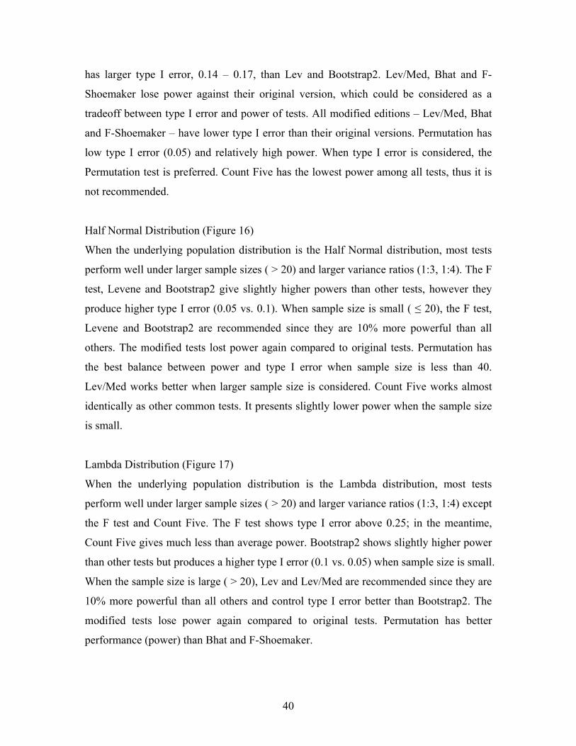
Half Normal Distribution (Figure 16)
When the underlying population distribution is the Half Normal distribution, most tests
perform well under larger sample sizes ( > 20) and larger variance ratios (1:3, 1:4). The F
test, Levene and Bootstrap2 give slightly higher powers than other tests, however they
produce higher type I error (0.05 vs. 0.1). When sample size is small ( ≤ 20), the F test,
Levene and Bootstrap2 are recommended since they are 10% more powerful than all
others. The modified tests lost power again compared to original tests. Permutation has
the best balance between power and type I error when sample size is less than 40.
Lev/Med works better when larger sample size is considered. Count Five works almost
identically as other common tests. It presents slightly lower power when the sample size
is small.
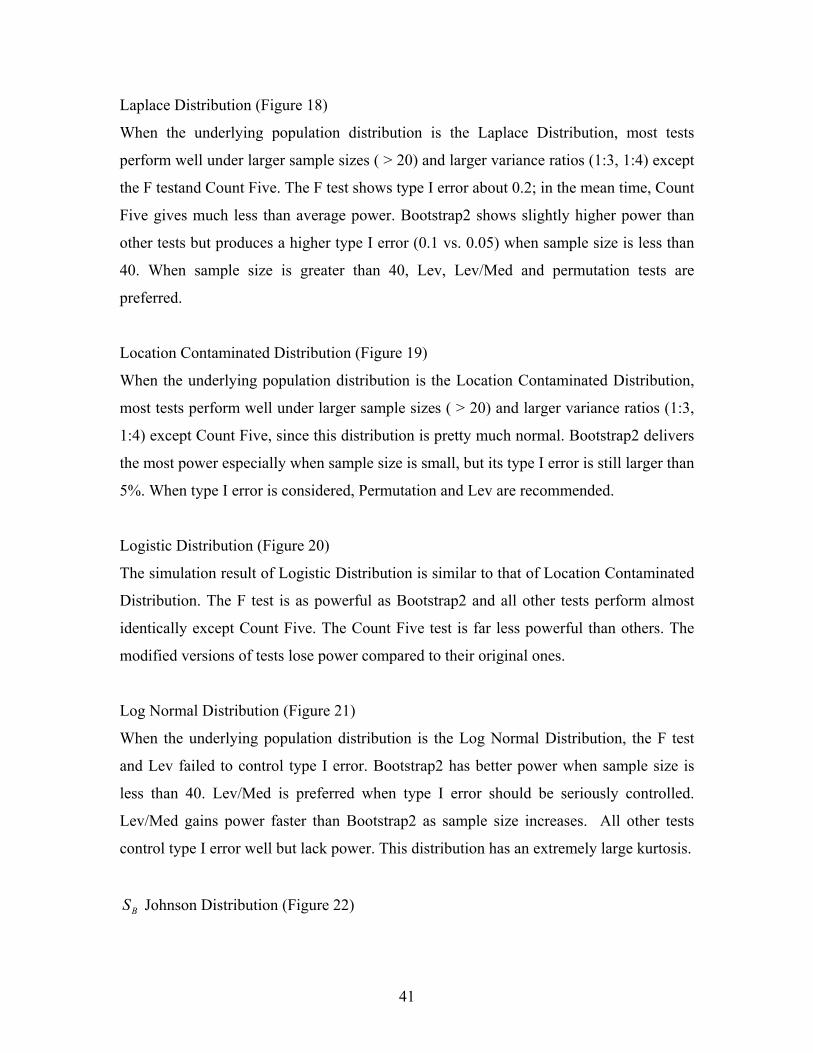
Lambda Distribution (Figure 17)
When the underlying population distribution is the Lambda distribution, most tests
perform well under larger sample sizes ( > 20) and larger variance ratios (1:3, 1:4) except
the F test and Count Five. The F test shows type I error above 0.25; in the meantime,
Count Five gives much less than average power. Bootstrap2 shows slightly higher power
than other tests but produces a higher type I error (0.1 vs. 0.05) when sample size is small.
When the sample size is large ( > 20), Lev and Lev/Med are recommended since they are
10% more powerful than all others and control type I error better than Bootstrap2. The
modified tests lose power again compared to original tests. Permutation has better
performance (power) than Bhat and F-Shoemaker.
40
Laplace Distribution (Figure 18)
When the underlying population distribution is the Laplace Distribution, most tests
perform well under larger sample sizes ( > 20) and larger variance ratios (1:3, 1:4) except
the F testand Count Five. The F test shows type I error about 0.2; in the mean time, Count
Five gives much less than average power. Bootstrap2 shows slightly higher power than
other tests but produces a higher type I error (0.1 vs. 0.05) when sample size is less than
40. When sample size is greater than 40, Lev, Lev/Med and permutation tests are
preferred.
Location Contaminated Distribution (Figure 19)
When the underlying population distribution is the Location Contaminated Distribution,
most tests perform well under larger sample sizes ( > 20) and larger variance ratios (1:3,
1:4) except Count Five, since this distribution is pretty much normal. Bootstrap2 delivers
the most power especially when sample size is small, but its type I error is still larger than
5%. When type I error is considered, Permutation and Lev are recommended.
Logistic Distribution (Figure 20)
The simulation result of Logistic Distribution is similar to that of Location Contaminated
Distribution. The F test is as powerful as Bootstrap2 and all other tests perform almost
identically except Count Five. The Count Five test is far less powerful than others. The
modified versions of tests lose power compared to their original ones.
Log Normal Distribution (Figure 21)
When the underlying population distribution is the Log Normal Distribution, the F test
and Lev failed to control type I error. Bootstrap2 has better power when sample size is
less than 40. Lev/Med is preferred when type I error should be seriously controlled.
Lev/Med gains power faster than Bootstrap2 as sample size increases. All other tests
control type I error well but lack power. This distribution has an extremely large kurtosis.
BS Johnson Distribution (Figure 22)
41

When the underlying population distribution is the Johnson Distribution, most tests
perform well under larger sample sizes ( > 20) and larger variance ratios (1:3, 1:4). Bhat
and F-Shoemaker tests are conservative and have relatively low power. The F test, Lev,
Bootstrap2 and Count Five show the best performance when sample size is small. We
were surprised to see the F test controls type I error well and Count Five test shows high
power also under this distribution. The distribution under these parameters is skewed
with low kurtosis.
BS
BS
Student T Distribution (Figure 23)
When the underlying population distribution is the Student T Distribution, once again
Lev, Lev/Med and Bootstrap2 show the best performance. Type I error is under control
and high power is presented. Bhat and Permutation give moderate results; they show
moderate power under all situations. F-shoemaker and Count Five give the lowest power
and they are not preferred. The F test presents much higher type I error than all other tests.
(0.25 vs. 0.05)
Tukey Distribution (Figure 24)
When the underlying population distribution is the Tukey T Distribution, Bootstrap2
shows the best performance. The F test shows highest power and also the highest type I
error. Bootstrap2 has a slightly higher type I error and higher power than the others.
Weibull (0.5) (Figure 25)
When the underlying population distribution is the Weibull(0.5) distribution, the F test,
Lev and Bootstrap2 are the most powerful tests among ten tests under all situations.
However, the F test and Lev have larger type I errors (0.25 – 0.6) than Bootstrap2. All
other tests show low power in this simulation. Lev/Med, Bhat and F-Shoemaker lose
power against their original versions. No test provides a satisfactory performance under
this high kurtosis distribution.
Normal (Figure 26)
Simulation result of Normal distribution is provided as a reference to all distributions.
42

Type I Error and Power of tests. X axis shows variance ratios and sample sizes.
Chi-Sqr(1)
0 0.1
0.2
0.3
0.4
0.5
0.6
0.7
0.8
0.9
1
1:1 1:2 1:3 1:4 1:1 1:2 1:3 1:4 1:1 1:2 1:3 1:4
Sample size 20 Sample size 40 Sample size 60
Pow
er o
f Tes
ts
Lev Lev/med Count 5 Bart Bhat F F-Sh Boot Boot 2 Permu
Figure 13 Simulation Result Distribution 2χ
Su Johnson
0
0.1
0.2
0.3
0.4
0.5
0.6
0.7
0.8
0.9
1
1:1 1:2 1:3 1:4 1:1 1:2 1:3 1:4 1:1 1:2 1:3 1:4
Sample size 20 Sample size 40 Sample size 60
Pow
er o
f Tes
ts
Lev
Lev/med
Count 5
Bart
Bhat
F
F-Sh
Boot
Boot 2
Permu
Figure 14 Simulation Result Distribution US
43

Extreme
0
0.2
0.4
0.6
0.8
1
1.2
1:1 1:2 1:3 1:4 1:1 1:2 1:3 1:4 1:1 1:2 1:3 1:4
Sample size 20 Sample size 40 Sample size 60
Pow
er o
f Tes
tsLev
Lev/med
Count 5
Bart
Bhat
F
F-Sh
Boot
Boot 2
Permu
Figure 15 Simulation Result Extreme Distribution
Half Normal
0
0.2
0.4
0.6
0.8
1
1.2
1:1 1:2 1:3 1:4 1:1 1:2 1:3 1:4 1:1 1:2 1:3 1:4
Sample size 20 Sample size 40 Sample size 60
Pow
er o
f Tes
ts
Lev
Lev/med
Count 5
Bart
Bhat
F
F-Sh
Boot
Boot 2
Permu
Figure 16 Simulation Result Half Normal Distribution
44

Lambda
0
0.1
0.2
0.3
0.4
0.5
0.6
0.7
0.8
0.9
1
1:1 1:2 1:3 1:4 1:1 1:2 1:3 1:4 1:1 1:2 1:3 1:4
Sample size 20 Sample size 40 Sample size 60
Pow
er o
f Tes
tsLev
Lev/med
Count 5
Bart
Bhat
F
F-Sh
Boot
Boot 2
Permu
Figure 17 Simulation Result Lambda Distribution
Laplace
0
0.2
0.4
0.6
0.8
1
1.2
1:1 1:2 1:3 1:4 1:1 1:2 1:3 1:4 1:1 1:2 1:3 1:4
Sample size 20 Sample size 40 Sample size 60
Pow
er o
f Tes
ts
Lev
Lev/med
Count 5
Bart
Bhat
F
F-Sh
Boot
Boot 2
Permu
Figure 18 Simulation Result Laplace Distribution
45

Local Con
0
0.2
0.4
0.6
0.8
1
1.2
1:1 1:2 1:3 1:4 1:1 1:2 1:3 1:4 1:1 1:2 1:3 1:4
Sample size 20 Sample size 40 Sample size 60
Pow
er o
f Tes
tsLev
Lev/med
Count 5
Bart
Bhat
F
F-Sh
Boot
Boot 2
Permu
Figure 19 Simulation Result Location Contaminated Distribution
Logistic
0
0.2
0.4
0.6
0.8
1
1.2
1:1 1:2 1:3 1:4 1:1 1:2 1:3 1:4 1:1 1:2 1:3 1:4
Sample size 20 Sample size 40 Sample size 60
Pow
er o
f Tes
ts
Lev
Lev/med
Count 5
Bart
Bhat
F
F-Sh
Boot
Boot 2
Permu
Figure 20 Simulation Result Logistic Distribution
46

Log Normal
0
0.1
0.2
0.3
0.4
0.5
0.6
0.7
0.8
0.9
1:1 1:2 1:3 1:4 1:1 1:2 1:3 1:4 1:1 1:2 1:3 1:4
Sample size 20 Sample size 40 Sample size 60
Pow
er o
f Tes
tsLev
Lev/med
Count 5
Bart
Bhat
F
F-Sh
Boot
Boot 2
Permu
Figure 21 Simulation Result Log Normal Distribution
Sb Johnson
0
0.2
0.4
0.6
0.8
1
1.2
1:1 1:2 1:3 1:4 1:1 1:2 1:3 1:4 1:1 1:2 1:3 1:4
Sample size 20 Sample size 40 Sample size 60
Pow
er o
f Tes
ts
Lev
Lev/med
Count 5
Bart
Bhat
F
F-Sh
Boot
Boot 2
Permu
Figure 22 Simulation Result Distribution BS
47

Student T
0
0.2
0.4
0.6
0.8
1
1.2
1:1 1:2 1:3 1:4 1:1 1:2 1:3 1:4 1:1 1:2 1:3 1:4
Sample size 20 Sample size 40 Sample size 60
Pow
er o
f Tes
tsLev
Lev/med
Count 5
Bart
Bhat
F
F-Sh
Boot
Boot 2
Permu
Figure 23 Simulation Result Student T Distribution
Tukey
0
0.2
0.4
0.6
0.8
1
1.2
1:1 1:2 1:3 1:4 1:1 1:2 1:3 1:4 1:1 1:2 1:3 1:4
Sample size 20 Sample size 40 Sample size 60
Pow
er o
f Tes
ts
Lev
Lev/med
Count 5
Bart
Bhat
F
F-Sh
Boot
Boot 2
Permu
Figure 24 Simulation Result Tukey Distribution
48

Weibull
0
0.1
0.2
0.3
0.4
0.5
0.6
0.7
0.8
0.9
1:1 1:2 1:3 1:4 1:1 1:2 1:3 1:4 1:1 1:2 1:3 1:4
Sample size 20 Sample size 40 Sample size 60
Pow
er o
f Tes
tsLev
Lev/med
Count 5
Bart
Bhat
F
F-Sh
Boot
Boot 2
Permu
Figure 25 Simulation Result Weibull Distribution
Normal
0
0.2
0.4
0.6
0.8
1
1.2
1:1 1:2 1:3 1:4 1:1 1:2 1:3 1:4 1:1 1:2 1:3 1:4
Sample size 20 Sample size 40 Sample size 60
Pow
er o
f Tes
ts
Lev
Lev/med
Count 5
Bart
Bhat
F
F-Sh
Boot
Boot 2
Permu
Figure 26 Simulation Result Normal Distribution
49

5 CONCLUSIONS
The Bootstrap method shows a consistent performance. For the nominal type I
errors of 0.05 in the simulation, the empirical type I errors are at most 0.1 and
its power is always among the highest.
Levene’s test achieves its best performance when the underlying distribution
has low kurtosis.
All modified editions – Lev/Med, Bhat and F-Shoemaker – have lower type I
error than their original versions.
Except F test and Bartlett’s test, all other tests control type I error pretty well. In
the meantime, the F test and Bartlett’s test present exceptionally high power in
simulations. However, they cannot be compared with the others because of their
poor control of type I error. Considering their high probability of type I error,
these two tests actually reject most situations.
Bootstrap and Lev/Med keep the best balance between type I error and power of
the test. Bootstrap works slightly better at smaller sample sizes ( ≤20), Lev/Med
has a better control of type I error (4% vs. 10%).
The Permutation test and Lev/Med are the two best choices when strict control
of type I error is required. Lev/Med has a slightly higher power than the
Permutation test.
No tests work well under high kurtosis distribution.
The Count Five method is simple but its performance is very poor when kurtosis
of distribution is not very small (< 3.0).
50

REFERENCES
[1] B.R. Bhat, M.N. Balade, and K.A. Rao, A New test for Equality of Variances for k
Normal Populations. Commun. Statist. –Simula.,31(4) (2002), 567-587
[2] D.D. Boos and C. Brownie, Comparing Variances and Other Measures of Dispersion.
Statistical Science (2004), Vol. 19, No. 4, 571–578
[3] D.D. Boos and C. Brownie, Bootstrap methods for testing homogeneity of variances.
Technometrics 31 (1989) 69–82.
[4] D.D. Boos, P. Janssen, and N. Veraverbeke, Resampling from centered data in the
two-sample problem. J. Statist. Plann. Inference 21 (1989) 327–345.
[5] G.E. Box and S.L. Andersen, Permutation theory in the derivation of robust criteria
and the study of departures from assumption (with discussion). J. Roy. Statist. Soc.
Ser. B 17 (1955) 1–34.
[6] M.B. Brown and A.B. Forsythe, Robust tests for the equality of variances. J. Amer.
Statist. Assoc. 69 (1974) 364–367.
[7] B. Efron, Bootstrap methods: another look at the jackknife. Ann. Statist. 7, (1979) 1-
26
[8] B. Efron and R.J. Tibshirani, An Introduction to the Bootstrap. Chapman & Hall/CRC.
[9] P. Hall, The Bootstrap and Edgeworth Expansion, Springer-Verlag, New York, 1992
[10] R.V. Hogg and E.A. Tanis, Probability and Statistical Inference. 5th Edition.
Prentice Hall, NJ, 1997
51

[11] N. L. Johnson, Systems of Frequency Curves Generated by Methods of
Translation.Biometrika Vol. 36,No. 1/2 (1949), pp. 149-176
[12] Kotz, Johnson, and Balakrishan, Continuous Univariate Distributions, Volumes I
and II, 2nd Edition. John Wiley and Sons, 1994
[13] H. Levene, Robust tests for equality of variances. In Contributions to Probability
and Statistics (I. Olkin, ed.) 278–292. Stanford Univ. Press, Stanford, CA, 1960
[14] B.F.J.R. Manly, Randomization, Bootstrap and Monte Carlo Methods in Biology. 2nd
Edition. Chapman & Hall, 1997
[15] R.N. Mcgrath and A.B. Yeh, A Quick, Compact, Two-Sample Dispersion Test:
Count Five. Amer. Statist. Assoc.59 (2005) 47-53
[16] NIST/SEMATECH e-Handbook of Statistical Methods,
http://www.itl.nist.gov/div898/handbook/. June, 2006.
[17] E. Seier, Comparison of Tests for Univariate Normality. Interstat, (January 2002
issue) http://interstat.statjournals.net/YEAR/2002/articles/0201001.pdf
[18] L.H. Shoemaker, Fixing the F test for equal variances. Amer. Statist. 57 (2003) 105–
114.
[19] T. Vorapongsathorn, S. Taejaroenkul, and C. Viwatwongkasem, A comparison of
type I error and power of Bartlett’s test, Levene’s test and Cochran’s test under
violation of assumptions. Songklanakarin J. Sci. Technol. Vol. 26 No. 4 (2004). 537-
547
[20] B.J. Winer, Statistical principles in experimental design. 2nd Edition. New York:
McGraw-Hill, 1974.
52

VITA
ZHIQIANG MU Personal Data: Date of Birth: April 15, 1977
Place of Birth: Chongqing, China, People’s Republic of
Education: Master of Science in Mathematical Sciences, East Tennessee
State University, Johnson City, Tennessee; 08/2006
Master of Science in Computer Science, Wake Forest
University, Winston-Salem, North Carolina; 05/2003
Bachelor of Engineering, Electrical Engineering, University of
Electronic Science and Technology of China, Chengdu, P. R.
China; 07/1999
Professional Experience: Engineer, Southwestern Institute of Electronic Technology,
Chengdu, P. R. China; 07/1999⎯06/2001.
53