comparison of different facts controllers and various...
TRANSCRIPT
CHAPTER – 3
COMPARISON OF DIFFERENT FACTS CONTROLLERS AND VARIOUS INPUT SIGNALS

CHAPTER-3
COMPARISON OF DIFFERENT FACTS CONTROLLERS AND VARIOUS INPUT SIGNALS
3.1 INTRODUCTION Damping of power system oscillation is one of the main concerns in the power
system operation since many years [62, 63]. In the recent years, the fast progress in
the field of power electronics have opened new opportunities for the application of
Flexible AC Transmission Systems (FACTS) devices as one of the most effective
ways to improve power system operation controllability and power transfer limits
[64, 65]. Due to the development of FACTS devices, Static Var Compensator (SVC),
Static Synchronous Compensator (STATCOM) and Static Synchronous Series
Compensator (SSSC) are routinely used in modern power systems. Hence, these
FACTS controllers are considered in this chapter for comparison of power oscillation
damping performance [2, 5, 7 ].
SVC and STATCOM are members of FACTS family that are connected in
shunt with the system [4, 6]. Even though the primary purpose of SVC and
STATCOM is to support bus voltage by injecting (or absorbing) reactive power, it is
also capable of improving the power system stability [66]. When a shunt compensator
is present in a power system to support the bus voltage, a supplementary damping
controller could be designed to modulate the bus voltage in order to improve damping
of system oscillations [21, 67]. SSSC is voltage sourced based series compensator and
provides the virtual compensation of transmission line impedance by injecting the
controllable voltage in series with the transmission line. The ability of SSSC to
operate in capacitive as well as inductive mode makes it very effective in controlling
the power flow of the system [8, 9]. An auxiliary stabilizing signal can also be
superimposed on the power flow control function of the SSSC so as to improve power
system oscillation stability [31]. Applications of SSSC for power oscillation damping,
stability enhancement and frequency stabilization can be found in several references
[28, 68-70]. The influence of degree of compensation and mode of operation of SSSC
ChapterChapterChapterChapter----3 : 3 : 3 : 3 : Comparison Comparison Comparison Comparison oooof Difff Difff Difff Different FACTS Controllers erent FACTS Controllers erent FACTS Controllers erent FACTS Controllers aaaand Various Input Signalsnd Various Input Signalsnd Various Input Signalsnd Various Input Signals
62
on small disturbance and transient stability is also reported in the literature [71, 72].
Artificial intelligence-based approaches have been proposed recently to design a
FACTS-based supplementary damping controller. These approaches include Particle
Swarm Optimization [35, 73], Genetic Algorithm [21], Differential Evolution [36,
55], Multi-Objective Evolutionary Algorithm [74] etc.
In the design of an efficient and effective damping controller, selection of the
appropriate input signal is a primary issue. Input signal must give correct control
actions when a disturbance occurs in the power system. Most of the available
literatures on damping controller design are based on either local signal or remote
signal. Also the issues related to potential time delays due to sensor time constant and
signal transmission delays are hardly addressed in the literature. Despite significant
strides in the development of advanced control schemes over the past two decades, the
conventional lead–lag structure controller remains the controller’s of choice in many
industrial applications. The conventional lead–lag controller structure remains an
engineer’s preferred choice because of its structural simplicity, reliability and the
favorable ratio between performance and cost. Beyond these benefits, it also offers
simplified dynamic modeling, lower user-skill requirements and minimal
development effort, which are issues of substantial importance to engineering
practice. In view of the above, a lead–lag structure controller has been considered in
the present study to modulate the controller injected or applied voltage.
A number of conventional techniques have been reported in the literature
pertaining to design problems of lead-lag structure controller, namely the eigen value
assignment, mathematical programming, gradient procedure for optimization, and
also the modern control theory. Unfortunately, the conventional techniques are time
consuming as they are iterative and require heavy computation burden and slow
convergence. In addition, the search process is susceptible to be trapped in local
minima, and the solution obtained may not be optimal. The evolutionary methods
constitute an approach to search for the optimum solutions via some form of directed
random search process. A relevant characteristic of the evolutionary methods is that
they search for solutions without previous problem knowledge.
ChapterChapterChapterChapter----3 : 3 : 3 : 3 : Comparison Comparison Comparison Comparison oooof Difff Difff Difff Different FACTS Controllers erent FACTS Controllers erent FACTS Controllers erent FACTS Controllers aaaand Various Input Signalsnd Various Input Signalsnd Various Input Signalsnd Various Input Signals
63
Recently, Gravitational search algorithm (GSA) appeared as a promising
evolutionary technique for handling the optimization problems [56]. GSA has been
popular in academia and the industry mainly because of its intuitiveness, ease of
implementation, and the ability to effectively solve highly nonlinear optimization
problems that are typical of complex engineering systems. It has been reported in the
literature that GSA is more efficient in terms of CPU time and offers higher precision
with more consistent results [37, 56]. In view of the above, this chapter proposes to
use GSA optimization technique for the damping controller design. In recent years,
the fast development of communication technology, low price communication devices
and various communication media makes it possible to provide the control center with
the real time signals from remote areas. However, the use of centralized controller
entails inputs that may arrive after a certain time delay. Time delays can make the
control system less effective. In order to satisfy specifications for wide-area control
systems, the design of a controller should take into account this time delay in order to
provide a controller that is robust, not only for the range of operating conditions
desired, but also for the uncertainty in delay. Recently there is a growing interest in
designing the controllers in the presence of uncertain time delays [75, 76, 77]. In view
of the above, this chapter investigates the design of various FACTS based damping
controller considering the potential time delays. Line active power as local signal and
speed deviation as remote signal are considered as candidate input signals for the
proposed FACTS based damping controllers. For controller design, Gravitational
Search Algorithm is employed due to its superior performance as presented in Chapter
2. To show the robustness of the proposed design approach, simulation results are
presented under various disturbance and faults for both SMIB and multi-machine
power system. Also, a comparison has been made between remote and local signal
and results are presented and analyzed.
The main objectives of the research work presented in this chapter are as follows:
1. To compare the damping performance of various FACTS controllers such as:
SVC, STATCOM and SSSC in a SMIB power system.
2. To investigate the effect of controller input signals (both local and remote) on
the performance of various FACTS based controller.

ChapterChapterChapterChapter----3 : 3 : 3 : 3 : Comparison Comparison Comparison Comparison oooof Difff Difff Difff Different FACTS Controllers erent FACTS Controllers erent FACTS Controllers erent FACTS Controllers aaaand Various Input Signalsnd Various Input Signalsnd Various Input Signalsnd Various Input Signals
64
3. To investigate the effect of potential time delays on the performance of
various FACTS based controller.
4. To design the FACTS based controller in a multi-machine power system.
3.2 SYSTEM UNDER STUDY
3.2.1 SMIB POWER SYSTEM WITH SVC AND STATCOM
The Single Machine Infinite Bus (SMIB) power system installed with a
SVC/STATCOM as shown in Fig. 3.1 is considered in this study. In Fig. 3.1, T1 and
T2 represents the main transformer and coupling transformer respectively, VT and VB
are the generator terminal and infinite-bus voltages, respectively, VSVC/STATCOM is the
bus voltages where shunt FACTS device is connected respectively, I is the line
current and PL and PL1 are the total real power flow in the transmission lines and that
in one line, respectively. The modeling of important power system components for
stability studies have already been given in Chapter 2. All the relevant parameters are
given in Appendix-II.
Load
STATCOMSVCV /TV
BV
Tr. lineT1
SVC/STATCOM
Generator
Bus-1Bus-2 Bus-3
ShuntFACTSDevices
T2
I PLPL1
Fig. 3.1 Single-machine infinite-bus power system with SVC/STATCOM

ChapterChapterChapterChapter----3 : 3 : 3 : 3 : Comparison Comparison Comparison Comparison oooof Difff Difff Difff Different FACTS Controllers erent FACTS Controllers erent FACTS Controllers erent FACTS Controllers aaaand Various Input Signalsnd Various Input Signalsnd Various Input Signalsnd Various Input Signals
65
3.2.2 OVERVIEW OF SVC AND ITS CONTROL SYSTEM
SVC is basically a shunt connected Static Var Generator whose output is
adjusted to exchange capacitive or inductive current so as to maintain or control
specific power system variables. Fig. 3.2 shows the single-line diagram of a SVC and
a simplified block diagram of its control system.
The control system consists of [57]:
• A measurement system measuring the positive-sequence voltage to be
controlled.
• A voltage regulator that uses the voltage error (difference between the
measured voltage Vm and the reference voltage (Vref) to determine the SVC
susceptance needed to keep the system voltage constant.
• A distribution unit that determines the Thyristor Switched Capacitors (TSC)
and eventually Thyristor Switched Reactors (TSR) that must be switched in
and out, and computes the firing angle α of TCRs.
A synchronizing system using a Phase-Locked Loop (PLL) synchronized on the
secondary voltages and a pulse generator that send appropriate pulses to the thyristors.
VoltageMeasurement
Synchronizing Unit(PLL)
Pulse Generator
Distributionunit
VoltageRegulator∑
Pulse
TCR TSC
Primary voltage mV
refV
α
+−
Secondary voltage
Fig. 3.2 Single-line diagram of control system of SVC

ChapterChapterChapterChapter----3 : 3 : 3 : 3 : Comparison Comparison Comparison Comparison oooof Difff Difff Difff Different FACTS Controllers erent FACTS Controllers erent FACTS Controllers erent FACTS Controllers aaaand Various Input Signalsnd Various Input Signalsnd Various Input Signalsnd Various Input Signals
66
3.2.3 OVERVIEW OF STATCOM AND ITS CONTROL SYSTEM
A Static Synchronous Compensator (STATCOM) is a controlled reactive-
power source. It provides voltage support by generating or absorbing reactive power
at the point of common coupling without the need of large external reactors or
capacitor banks [2]. The basic electronic block of a STATCOM is the Voltage
Sourced Converter (VSC), which in general converts an input dc voltage into a three-
phase output voltage at fundamental frequency, with rapidly controllable amplitude
and phase angle. In addition to this, the controller has a coupling transformer and a dc
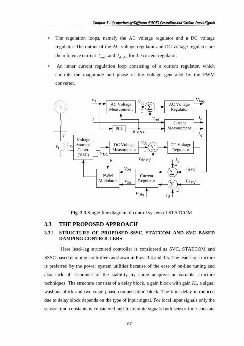
capacitor. Fig. 3.3 shows the single-line diagram of a STATCOM and a simplified
block diagram of its control system. In Fig. 3.3, references fQ eR and fP eR define the
magnitude and phase angle of the converter voltage cnvV necessary to exchange the
desired reactive and active power between the solid state voltage sourced converter
and the ac system. If the device is operated strictly for reactive power exchange, fPRe
is set to zero and the external energy source is not required. The converter voltage
cnvV is in phase with the ac terminal voltage acV and there is practically no real power
flow from or to VSC (without energy storage). The STATCOM supplies reactive
power to the ac system if cnvV is greater than acV and consumes reactive power if cnvV
is lower than acV .The device can be designed to maintain the magnitude of the bus
voltage constant by controlling the magnitude and/or phase shift of the VSC output
voltage.
The control system consists of:
• A Phase-Locked Loop (PLL) to synchronize on the positive-sequence
component of the 3-phase primary voltage 1V . The direct-axis and quadrature-
axis components of the AC 3-phase voltage and currents (labeled as dV , qV and
dI , qI on the diagram) are computed using the output of the PLL.
• The measurement systems measuring the d-axis and q-axis components of AC
positive-sequence voltage and currents to be controlled as well as the DC
voltage DCV .
ChapterChapterChapterChapter----3 : 3 : 3 : 3 : Comparison Comparison Comparison Comparison oooof Difff Difff Difff Different FACTS Controllers erent FACTS Controllers erent FACTS Controllers erent FACTS Controllers aaaand Various Input Signalsnd Various Input Signalsnd Various Input Signalsnd Various Input Signals
67
• The regulation loops, namely the AC voltage regulator and a DC voltage
regulator. The output of the AC voltage regulator and DC voltage regulator are
the reference current refqI and refdI , for the current regulator.
• An inner current regulation loop consisting of a current regulator, which
controls the magnitude and phase of the voltage generated by the PWM
converter.
AC VoltageMeasurement
AC VoltageRegulator∑
PLLCurrent
Measurement
acV
refV
1V
I
tωθ =
dq1V
qI
dI
DC VoltageMeasurement
DC VoltageRegulator∑
VoltageSourcedConvt.(VSC)
1V 2V
I
DCV
dcV
refdcV
PWMModulator
CurrentRegulator
∑
∑
θ
d2V
q2V
qI
dI
refqI
refdI
dq1V
+
−+
−
+−
+−
Fig. 3.3 Single-line diagram of control system of STATCOM
3.3 THE PROPOSED APPROACH
3.3.1 STRUCTURE OF PROPOSED SSSC, STATCOM AND SVC BASED DAMPING CONTROLLERS
Here lead–lag structured controller is considered as SVC, STATCOM and
SSSC-based damping controllers as shown in Figs. 3.4 and 3.5. The lead-lag structure
is preferred by the power system utilities because of the ease of on-line tuning and
also lack of assurance of the stability by some adaptive or variable structure
techniques. The structure consists of a delay block, a gain block with gain KS, a signal
washout block and two-stage phase compensation block. The time delay introduced
due to delay block depends on the type of input signal. For local input signals only the
sensor time constants is considered and for remote signals both sensor time constant
ChapterChapterChapterChapter----3 : 3 : 3 : 3 : Comparison Comparison Comparison Comparison oooof Difff Difff Difff Different FACTS Controllers erent FACTS Controllers erent FACTS Controllers erent FACTS Controllers aaaand Various Input Signalsnd Various Input Signalsnd Various Input Signalsnd Various Input Signals
68
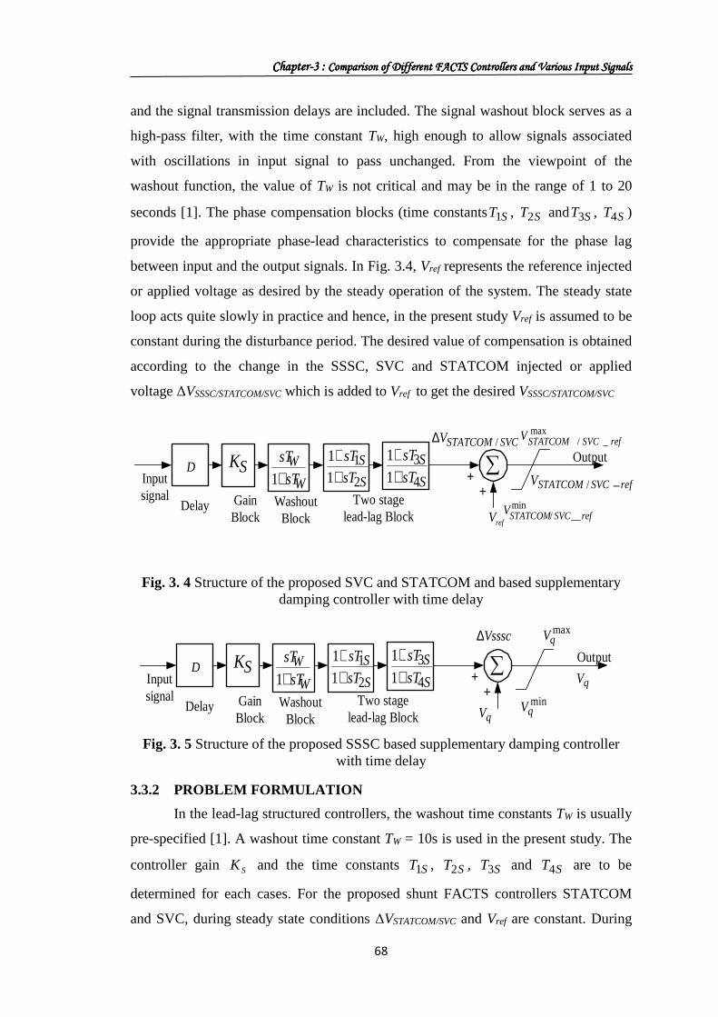
and the signal transmission delays are included. The signal washout block serves as a
high-pass filter, with the time constant TW, high enough to allow signals associated
with oscillations in input signal to pass unchanged. From the viewpoint of the
washout function, the value of TW is not critical and may be in the range of 1 to 20
seconds [1]. The phase compensation blocks (time constants ST1 , ST2 and ST3 , ST4 )
provide the appropriate phase-lead characteristics to compensate for the phase lag
between input and the output signals. In Fig. 3.4, Vref represents the reference injected
or applied voltage as desired by the steady operation of the system. The steady state
loop acts quite slowly in practice and hence, in the present study Vref is assumed to be
constant during the disturbance period. The desired value of compensation is obtained
according to the change in the SSSC, SVC and STATCOM injected or applied
voltage ∆VSSSC/STATCOM/SVC which is added to Vref to get the desired VSSSC/STATCOM/SVC
SKW
WsT
sT
+1 S
SsT
sT
2
111++
S
SsT
sT
4
311++
Inputsignal Gain
BlockWashout
BlockTwo stage
lead-lag Block
Output
refSVCSTATCOMV _/
refV
++
max_/ refSVCSTATCOMV
∑D
Delay
SVCSTATCOMV /∆
min__/ refSVCSTATCOMV
Fig. 3. 4 Structure of the proposed SVC and STATCOM and based supplementary damping controller with time delay
SKW
WsT
sT
+1 S
SsT
sT
2
111++
S
SsT
sT
4
311++
Inputsignal Gain
BlockWashout
BlockTwo stage
lead-lag Block
Output
qV
qV
++
maxqV
∑D
Delay
Vsssc∆
minqV
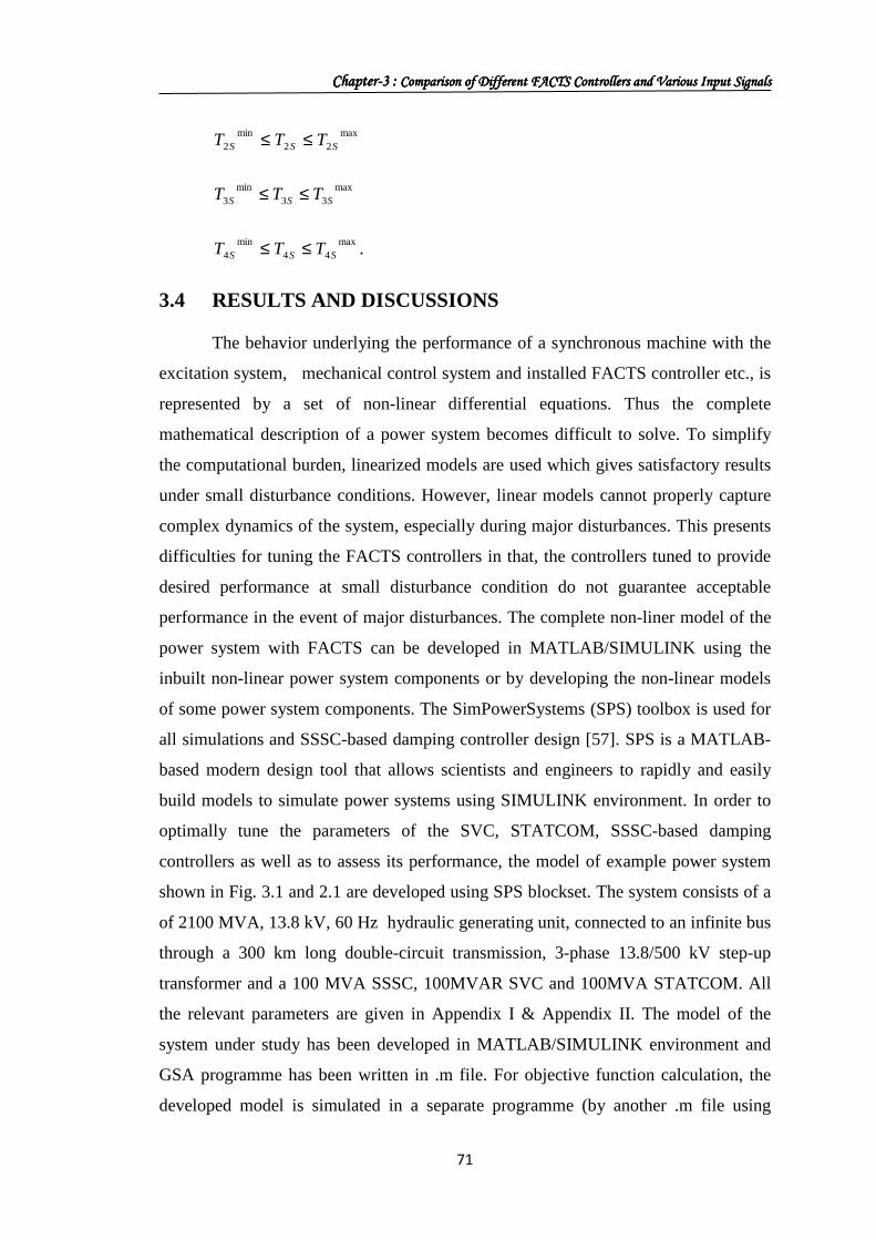
Fig. 3. 5 Structure of the proposed SSSC based supplementary damping controller
with time delay
3.3.2 PROBLEM FORMULATION In the lead-lag structured controllers, the washout time constants TW is usually
pre-specified [1]. A washout time constant TW = 10s is used in the present study. The
controller gain SK and the time constants ST1 , ST2 , ST3 and ST4 are to be
determined for each cases. For the proposed shunt FACTS controllers STATCOM
and SVC, during steady state conditions ∆VSTATCOM/SVC and Vref are constant. During

ChapterChapterChapterChapter----3 : 3 : 3 : 3 : Comparison Comparison Comparison Comparison oooof Difff Difff Difff Different FACTS Controllers erent FACTS Controllers erent FACTS Controllers erent FACTS Controllers aaaand Various Input Signalsnd Various Input Signalsnd Various Input Signalsnd Various Input Signals
69
dynamic conditions the reference voltage ∆VSTATCOM/SVC are modulated to damp
system oscillations. The effective reference voltage VSTATCOM/SVC_ref in dynamic
conditions is given by:
SVCSTATCOMefrrefSVCSTATCOM VVV /_/ ∆+= (3.1)
For the case of SSSC controller during steady state conditions ∆VSSSC and Vq
are constant. During dynamic conditions the injected voltage ∆VSSSC are modulated to
damp system oscillations. The effective injected voltage VSSSC in dynamic conditions
is given by:
SSSCqqSSSC VVV ∆+=_ (3.2)
In the design of a robust damping controller, selection of the appropriate
input signal is a main issue. Input signal must give correct control actions when a
disturbance occurs in the power system. Both local and remote signals can be used as
control. To avoid additional costs associated with communication and to improve
reliability, input signal should preferably be locally measurable. However, local
control signals, although easy to get, may not contain the desired oscillation modes.
So, compared to wide-area signals, they are not as highly controllable and observable.
Owing to the recent advances in optical fiber communication and global positioning
systems, the wide-area measurement system can realize phasor measurement
synchronously and deliver it to the control center even in real time, which makes the
wide-area signal a good alternative for control input. In a wide-area monitoring
system, global positioning system synchronized time-stamped data are used. In
today’s technology, dedicated communication channels should not have more than
50-ms delay for the transmission of measured signals even in the worst scenarios
[101]. For local input signals, line active power, line reactive power, line current
magnitude and bus voltage magnitudes are all candidates to be considered in the
selection of input signals for the FACTS power oscillation damping controller.
Among these possible local input signals, active power and current are the most
commonly employed in the literature. Similarly, generator rotor angle and speed
deviation can be used as remote signals. However rotor speed seems to be a better
alternative as input signal for FACTS based controller [102] In view of the above,

ChapterChapterChapterChapter----3 : 3 : 3 : 3 : Comparison Comparison Comparison Comparison oooof Difff Difff Difff Different FACTS Controllers erent FACTS Controllers erent FACTS Controllers erent FACTS Controllers aaaand Various Input Signalsnd Various Input Signalsnd Various Input Signalsnd Various Input Signals
70
both line active power and speed deviations are considered and compared as candidate
input signals for the SSSC/STATCOM/SVC based controller. For local signals a
sensor time constant of 15 ms is considered. For remote signals a signal transmission
delay of 50 ms is considered along with the sensor time constant of 15 ms. In the
present study, an integral time absolute error of the speed deviations is taken as the
objective function J expressed as:
∫=
=
⋅⋅∆=simtt
t
dttJ0
|| ω (3.3)
Where, ∆ω is the speed deviation in and tsim is the time range of the simulation.
During normal operating condition there is complete balance between input
mechanical power and output electrical power and this is true for all operating points.
During disturbance, the balance is disturbed and the difference power enters
into/drawn from the rotor. Hence the rotor speed deviation and subsequently all other
parameters (power, current, voltage etc.) change. As the input to the SSSC/
STATCOM/ SVC based controller is the speed deviation/electrical power, the SSSC
injected voltage and STATCOM/SVC injected currents are suitable modulated and
the power balanced is maintained at the earliest time period irrespective of the
operating point. So, with the change in operating point also the SSSC/STATCOM/
SVC based controller parameters remain fixed.
For objective function calculation, the time-domain simulation of the power
system model is carried out for the simulation period. It is aimed to minimize this
objective function in order to improve the system response in terms of the settling
time and overshoots. The problem constraints are the SSSC/STATCOM/SVC
controller’s parameter bounds. Therefore, the design problem can be formulated as
the following optimization problem.
Minimize J (3.4)
Subject to
maxminSSS KKK ≤≤
max11
min1 SSS TTT ≤≤
ChapterChapterChapterChapter----3 : 3 : 3 : 3 : Comparison Comparison Comparison Comparison oooof Difff Difff Difff Different FACTS Controllers erent FACTS Controllers erent FACTS Controllers erent FACTS Controllers aaaand Various Input Signalsnd Various Input Signalsnd Various Input Signalsnd Various Input Signals
71
max22
min2 SSS TTT ≤≤
max33
min3 SSS TTT ≤≤
max44
min4 SSS TTT ≤≤ .
3.4 RESULTS AND DISCUSSIONS
The behavior underlying the performance of a synchronous machine with the
excitation system, mechanical control system and installed FACTS controller etc., is
represented by a set of non-linear differential equations. Thus the complete
mathematical description of a power system becomes difficult to solve. To simplify
the computational burden, linearized models are used which gives satisfactory results
under small disturbance conditions. However, linear models cannot properly capture
complex dynamics of the system, especially during major disturbances. This presents
difficulties for tuning the FACTS controllers in that, the controllers tuned to provide
desired performance at small disturbance condition do not guarantee acceptable
performance in the event of major disturbances. The complete non-liner model of the
power system with FACTS can be developed in MATLAB/SIMULINK using the
inbuilt non-linear power system components or by developing the non-linear models
of some power system components. The SimPowerSystems (SPS) toolbox is used for
all simulations and SSSC-based damping controller design [57]. SPS is a MATLAB-
based modern design tool that allows scientists and engineers to rapidly and easily
build models to simulate power systems using SIMULINK environment. In order to
optimally tune the parameters of the SVC, STATCOM, SSSC-based damping
controllers as well as to assess its performance, the model of example power system
shown in Fig. 3.1 and 2.1 are developed using SPS blockset. The system consists of a
of 2100 MVA, 13.8 kV, 60 Hz hydraulic generating unit, connected to an infinite bus
through a 300 km long double-circuit transmission, 3-phase 13.8/500 kV step-up
transformer and a 100 MVA SSSC, 100MVAR SVC and 100MVA STATCOM. All
the relevant parameters are given in Appendix I & Appendix II. The model of the
system under study has been developed in MATLAB/SIMULINK environment and
GSA programme has been written in .m file. For objective function calculation, the
developed model is simulated in a separate programme (by another .m file using

ChapterChapterChapterChapter----3 : 3 : 3 : 3 : Comparison Comparison Comparison Comparison oooof Difff Difff Difff Different FACTS Controllers erent FACTS Controllers erent FACTS Controllers erent FACTS Controllers aaaand Various Input Signalsnd Various Input Signalsnd Various Input Signalsnd Various Input Signals
72
initial population/controller parameters) considering a disturbance. Form the
SIMULINK model the objective function value is evaluated and moved to workspace.
The process is repeated for each individual in the population. The optimization of the
proposed SVC, STATCOM, SSSC-based damping controller parameters is carried out
by minimizing the objective function given in Eq. (3.3) employing GSA. The
objective function value is evaluated for each individual by simulating the example
power system, considering a severe disturbance. For objective function calculation, a
3-phase short-circuit fault in one of the parallel transmission lines is considered.The
flow chart of the GSA algorithm employed in the present study is given in Fig. 1.13.
Simulations were conducted on a Pentium 4, 3 GHz, 504 MB RAM computer, in the
MATLAB 7.0.1 environment. The optimization was repeated 20 times and the best
final solution among the 20 runs is chosen as proposed controller parameters. The best
final solutions obtained in the 20 runs for different FACTS controllers with various
input signal are given in Table 3.1
To evaluate the capability of the SVC, STATCOM and SSSC based
controllers on damping electromechanical oscillations of the example electric power
system, simulations are carried out. To assess the effectiveness and robustness of the
controllers, different loading conditions as given in Table 3.2 are considered.
Table 3.1: SSSC, STATCOM and SVC based controller’s parameters for SMIB
Controllers Signal/Parameters SK ST1 ST2 ST3 ST4
SSSC Remote (∆ω) 115.4319 1.0029 0.8153 1.1482 0.8128
STATCOM Remote (∆ω) 493.8315 1.4315 0.8985 0.0626 1.6768
SVC Remote (∆ω) 203.7043 0.2132 1.2849 1.0672 0.9910
SSSC Local (∆PL) 89.0582 1.3945 0.8498 0.4673 0.1650
STATCOM Local (∆PL) 346.2304 1.3837 1.3491 1.2812 1.7203
SVC Local (∆PL) 344.5442 1.0824 1.0124 0.9874 1.1058

ChapterChapterChapterChapter----3 : 3 : 3 : 3 : Comparison Comparison Comparison Comparison oooof Difff Difff Difff Different FACTS Controllers erent FACTS Controllers erent FACTS Controllers erent FACTS Controllers aaaand Various Input Signalsnd Various Input Signalsnd Various Input Signalsnd Various Input Signals
73
Table 3.2: Operating conditions considered
Controllers Loading Conditions P (pu) δ0(deg.)
SSSC
STATCOM
SVC
Nominal 0.85 29.21
Light 0.5 55.52
Heavy 1 60.53
3.4.1 COMPARISON OF SVC, STATCOM AND SSSC BASED CONTROLLERS WITH REMOTE SIGNAL
A 3-phase fault is applied in the middle of transmission line at t=1sec and
cleared after 5-cycle under nominal loading condition. The variation of power angle δ,
speed deviation ∆ω and tie line power for the above contingency are shown in Figs.
3.6-3.8. It is clear from Figs. that when input to the controller is remote ∆ω, the
stability of the system are maintained with SVC, STATCOM and SSSC based
controllers and power system oscillations are effectively damped out. It can also be
seen from Figs. 3.6-3.8 STATCOM is slightly more effective than SVC from stability
point of view. It is also evident from Figs. 3.6-3.8 that best system response is
obtained with SSSC based damping controller.
0 1 2 3 4 5 6 7 8 9 10-6
-4
-2
0
2
4
6x 10
-3
Time (sec)
∆ω
(pu)
SVC STATCOM SSSC
Fig. 3.6 Speed deviation response for 5-cycle 3-phase fault in transmission line with nominal loading
ChapterChapterChapterChapter----3 : 3 : 3 : 3 : Comparison Comparison Comparison Comparison oooof Difff Difff Difff Different FACTS Controllers erent FACTS Controllers erent FACTS Controllers erent FACTS Controllers aaaand Various Input Signalsnd Various Input Signalsnd Various Input Signalsnd Various Input Signals
74
0 1 2 3 4 5 6 7 8 9 1035
40
45
50
55
60
65
Time (sec)
δ (d
egre
e)
SVC STATCOM SSSC
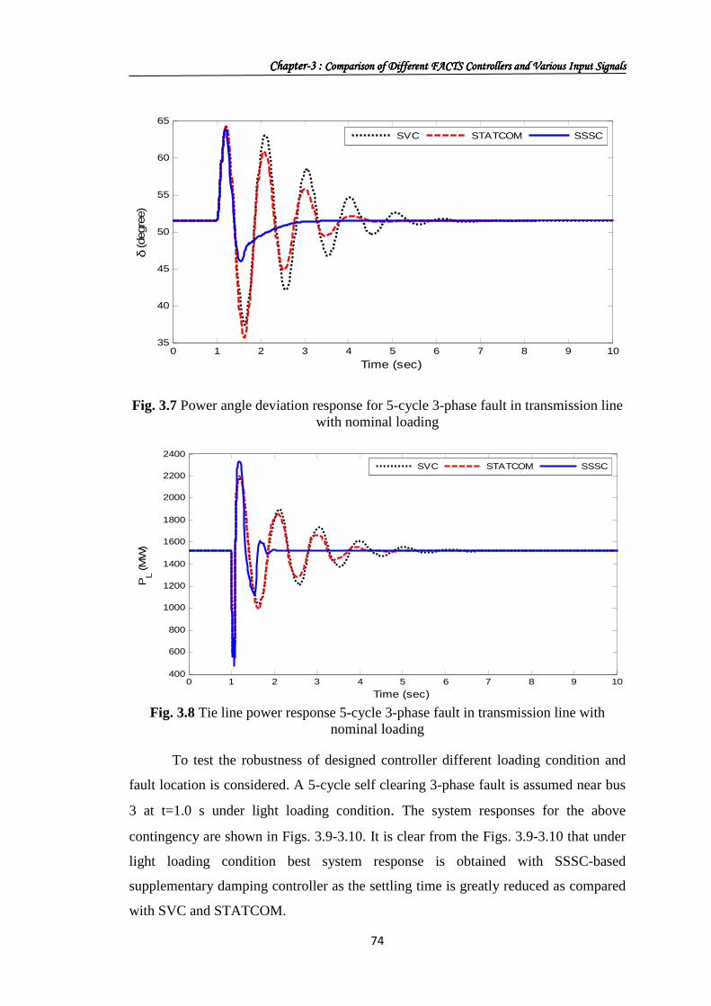
Fig. 3.7 Power angle deviation response for 5-cycle 3-phase fault in transmission line with nominal loading
0 1 2 3 4 5 6 7 8 9 10400
600
800
1000
1200
1400
1600
1800
2000
2200
2400
Time (sec)
PL (
MW
)
SVC STATCOM SSSC
Fig. 3.8 Tie line power response 5-cycle 3-phase fault in transmission line with nominal loading
To test the robustness of designed controller different loading condition and
fault location is considered. A 5-cycle self clearing 3-phase fault is assumed near bus
3 at t=1.0 s under light loading condition. The system responses for the above
contingency are shown in Figs. 3.9-3.10. It is clear from the Figs. 3.9-3.10 that under
light loading condition best system response is obtained with SSSC-based
supplementary damping controller as the settling time is greatly reduced as compared
with SVC and STATCOM.

ChapterChapterChapterChapter----3 : 3 : 3 : 3 : Comparison Comparison Comparison Comparison oooof Difff Difff Difff Different FACTS Controllers erent FACTS Controllers erent FACTS Controllers erent FACTS Controllers aaaand Various Input Signalsnd Various Input Signalsnd Various Input Signalsnd Various Input Signals
75
0 1 2 3 4 5 6 7 8 9 10-5
-4
-3
-2
-1
0
1
2
3
4
5x 10
-3
Time (sec)
∆ω (pu
)
SVC STATCOM SSSC
Fig. 3. 9 Speed deviation response for 5-cycle 3-phase fault in transmission line with light loading
0 1 2 3 4 5 6 7 810
15
20
25
30
35
40
45
Time (sec)
δ (d
egre
e)
SVC STATCOM SSSC
Fig. 3.10 Power angle deviation response for 5-cycle 3-phase fault in transmission line with light loading
The effectiveness of the proposed controllers is also tested under heavy
loading condition (given in Table 3.1) by applying a 5-cycle 3-phase fault disturbance
at Bus 2 which is cleared by tripping both lines. The system responses are shown in
Figs. 3.11-3.13. It can be seen from Figs. 3.11-3.13 that the proposed controllers are
robust and works effectively under various operating conditions. The best system
response is observed with SSSC controller compared to STATCOM and SVC
controllers.

ChapterChapterChapterChapter----3 : 3 : 3 : 3 : Comparison Comparison Comparison Comparison oooof Difff Difff Difff Different FACTS Controllers erent FACTS Controllers erent FACTS Controllers erent FACTS Controllers aaaand Various Input Signalsnd Various Input Signalsnd Various Input Signalsnd Various Input Signals
76
0 1 2 3 4 5 6 7 8 9 10-8
-6
-4
-2
0
2
4
6
8
10x 10
-4
Time (sec)
∆ω (pu
)
SVC STATCOM SSSC
Fig. 3.11 Speed deviation response for 5-cycle 3-phase fault disturbance at Bus 2
cleared by both line tripping with heavy loading
0 1 2 3 4 5 6 7 8 9 1058.5
59
59.5
60
60.5
61
61.5
62
62.5
63
63.5
Time (sec)
δ (deg
ree)
SVC STATCOM SSSC
Fig. 3.12 Power angle deviation response for 5-cycle 3-phase fault disturbance at Bus 2 cleared by both line tripping with heavy loading
0 1 2 3 4 5 6 7 8 9 101750
1800
1850
1900
1950
2000
2050
2100
Time (sec)
PL (
MW
)
SVC STATCOM SSSC
Fig. 3.13 Tie line power response for 5-cycle 3-phase fault disturbance at Bus 2
cleared by both line tripping with heavy loading

ChapterChapterChapterChapter----3 : 3 : 3 : 3 : Comparison Comparison Comparison Comparison oooof Difff Difff Difff Different FACTS Controllers erent FACTS Controllers erent FACTS Controllers erent FACTS Controllers aaaand Various Input Signalsnd Various Input Signalsnd Various Input Signalsnd Various Input Signals
77
3.4.2 COMPARISON OF SVC, STATCOM AND SSSC BASED CONTROLLERS WITH LOCAL SIGNAL
In order to verify the effectiveness of controllers with local input signal, the
performance of the SVC, STATCOM and SSSC with local line power deviation
( LP∆ ) input signal are tested for different loading conditions. The behavior of the
proposed controller is verified at nominal loading condition under severe disturbance
condition. A 5-cycle, 3-phase fault is applied at the middle of one transmission line
connecting bus 2 and bus 3, at t = 1.0 s. The fault is removed by opening the faulty
line and the lines are reclosed after 5-cycles. The system response under this severe
disturbance is shown in Figs. 3.14-3.16 where, the response with LP∆ -based SVC is
shown with dotted line, the response with proposed GSA optimized LP∆ -based
STATCOM dashed line and the response with LP∆ -based SSSC solid line. It is clear
that settling time and overshoots in case of LP∆ based SSSC based controller is
better than LP∆ based SVC and STATCOM controllers under nominal loading
condition.
0 1 2 3 4 5 6 7 8 9 10-8
-6
-4
-2
0
2
4
6
8x 10
-3
Time (sec)
∆ω (pu
)
SVC STATCOM SSSC
Fig. 3.14 Speed deviation response for 5-cycle 3-phase fault in transmission line with nominal loading
ChapterChapterChapterChapter----3 : 3 : 3 : 3 : Comparison Comparison Comparison Comparison oooof Difff Difff Difff Different FACTS Controllers erent FACTS Controllers erent FACTS Controllers erent FACTS Controllers aaaand Various Input Signalsnd Various Input Signalsnd Various Input Signalsnd Various Input Signals
78
0 1 2 3 4 5 6 7 8 9 1035
40
45
50
55
60
65
70
Time (sec)
δ (d
egre
e)
SVC STATCOM SSSC
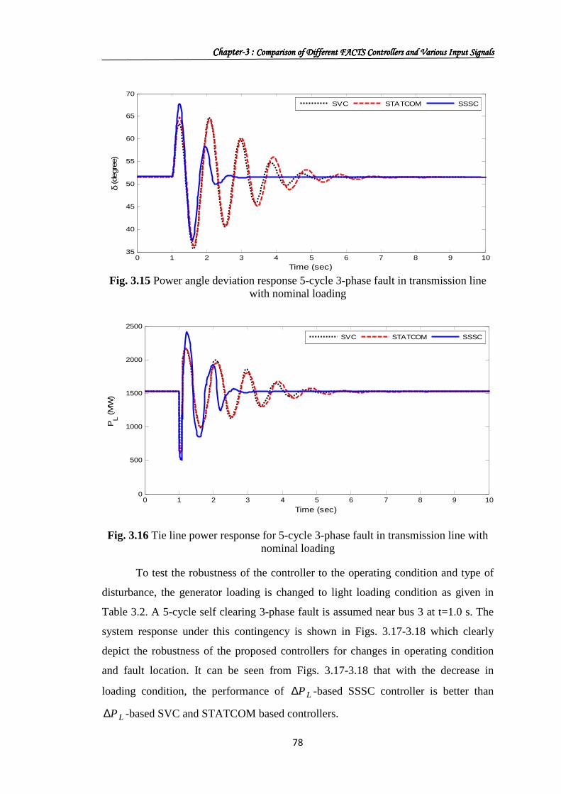
Fig. 3.15 Power angle deviation response 5-cycle 3-phase fault in transmission line with nominal loading
0 1 2 3 4 5 6 7 8 9 100
500
1000
1500
2000
2500
Time (sec)
PL (
MW
)
SVC STATCOM SSSC
Fig. 3.16 Tie line power response for 5-cycle 3-phase fault in transmission line with nominal loading
To test the robustness of the controller to the operating condition and type of
disturbance, the generator loading is changed to light loading condition as given in
Table 3.2. A 5-cycle self clearing 3-phase fault is assumed near bus 3 at t=1.0 s. The
system response under this contingency is shown in Figs. 3.17-3.18 which clearly
depict the robustness of the proposed controllers for changes in operating condition
and fault location. It can be seen from Figs. 3.17-3.18 that with the decrease in
loading condition, the performance of LP∆ -based SSSC controller is better than
LP∆ -based SVC and STATCOM based controllers.

ChapterChapterChapterChapter----3 : 3 : 3 : 3 : Comparison Comparison Comparison Comparison oooof Difff Difff Difff Different FACTS Controllers erent FACTS Controllers erent FACTS Controllers erent FACTS Controllers aaaand Various Input Signalsnd Various Input Signalsnd Various Input Signalsnd Various Input Signals
79
0 1 2 3 4 5 6 7 8 9 10-6
-4
-2
0
2
4
6x 10
-3
Time (sec)
∆ω (pu
)
SVC STATCOM SSSC
Fig. 3.17 Speed deviation response for 5-cycle 3-phase in transmission line with light
loading
0 1 2 3 4 5 6 7 8 9 1010
15
20
25
30
35
40
45
Time (sec)
δ (d
egre
e)
SVC STATCOM SSSC
Fig. 3.18 Power angle deviation response for 5-cycle 3-phase fault in transmission
line with light loading
The effectiveness of the proposed controller is also tested at heavy loading
condition under small disturbance. The load near bus 2 is disconnected at t =1.0 s for
5-cycle. The response of speed deviation and power angle deviation for this case is
shown in Figs. 3.19 and 3.20 respectively. It is observed from Figs. 3.19 and 3.20 that
proposed LP∆ -based SSSC gives better system response thanLP∆ based SVC and
STATCOM controllers. It is also shown that settling times are greatly reduced with
LP∆ based SSSC controller compared to others.

ChapterChapterChapterChapter----3 : 3 : 3 : 3 : Comparison Comparison Comparison Comparison oooof Difff Difff Difff Different FACTS Controllers erent FACTS Controllers erent FACTS Controllers erent FACTS Controllers aaaand Various Input Signalsnd Various Input Signalsnd Various Input Signalsnd Various Input Signals
80
0 1 2 3 4 5 6 7 8 9 10-8
-6
-4
-2
0
2
4
6
8x 10
-4
Time (sec)
∆ω (pu
)
SVC STATCOM SSSC
Fig. 3.19 Speed deviation response for 5-cycle 3-phase fault disturbance at Bus 2 cleared by both line tripping with heavy loading
0 1 2 3 4 5 6 7 8 9 1058.5
59
59.5
60
60.5
61
61.5
62
62.5
63
63.5
Time (sec)
δ (d
egre
e)
SVC STATCOM SSSC
Fig. 3.20 Power angle deviation response for 5-cycle 3-phase fault disturbance at Bus 2 cleared by both line tripping with heavy loading
3.4.3 COMPARISON OF CONTROLLERS WITH DIFFERENT SIGNALS In Section 3.4.1 and 3.4.2, a comparison is made between the SSSC,
STATCOM and SVC with both local and remote signals for stability enhancement of
the power system. It is observed that the SSSC based controller is more effective for
stability enhancement of the proposed system. In this Section, a comparison between
local and remote signal for SSSC based controller to improve the stability of power
system is carried out.
ChapterChapterChapterChapter----3 : 3 : 3 : 3 : Comparison Comparison Comparison Comparison oooof Difff Difff Difff Different FACTS Controllers erent FACTS Controllers erent FACTS Controllers erent FACTS Controllers aaaand Various Input Signalsnd Various Input Signalsnd Various Input Signalsnd Various Input Signals
81
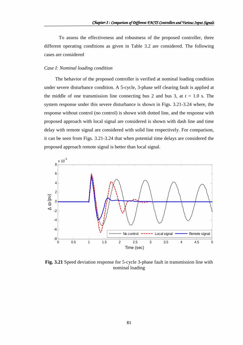
To assess the effectiveness and robustness of the proposed controller, three
different operating conditions as given in Table 3.2 are considered. The following
cases are considered
Case I: Nominal loading condition
The behavior of the proposed controller is verified at nominal loading condition
under severe disturbance condition. A 5-cycle, 3-phase self clearing fault is applied at
the middle of one transmission line connecting bus 2 and bus 3, at t = 1.0 s. The
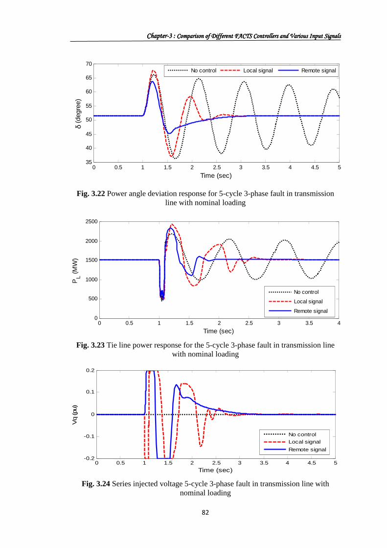
system response under this severe disturbance is shown in Figs. 3.21-3.24 where, the
response without control (no control) is shown with dotted line, and the response with
proposed approach with local signal are considered is shown with dash line and time
delay with remote signal are considered with solid line respectively. For comparison,
it can be seen from Figs. 3.21-3.24 that when potential time delays are considered the
proposed approach remote signal is better than local signal.
0 0.5 1 1.5 2 2.5 3 3.5 4 4.5 5-8
-6
-4
-2
0
2
4
6
8x 10
-3
Time (sec)
∆ ω
(pu)
No control Local signal Remote signal
Fig. 3.21 Speed deviation response for 5-cycle 3-phase fault in transmission line with nominal loading
ChapterChapterChapterChapter----3 : 3 : 3 : 3 : Comparison Comparison Comparison Comparison oooof Difff Difff Difff Different FACTS Controllers erent FACTS Controllers erent FACTS Controllers erent FACTS Controllers aaaand Various Input Signalsnd Various Input Signalsnd Various Input Signalsnd Various Input Signals
82
0 0.5 1 1.5 2 2.5 3 3.5 4 4.5 535
40
45
50
55
60
65
70
Time (sec)
δ (d
egre
e)
No control Local signal Remote signal
Fig. 3.22 Power angle deviation response for 5-cycle 3-phase fault in transmission line with nominal loading
0 0.5 1 1.5 2 2.5 3 3.5 40
500
1000
1500
2000
2500
Time (sec)
PL (
MW
)
No control
Local signal
Remote signal
Fig. 3.23 Tie line power response for the 5-cycle 3-phase fault in transmission line with nominal loading
0 0.5 1 1.5 2 2.5 3 3.5 4 4.5 5-0.2
-0.1
0
0.1
0.2
Time (sec)
Vq
(pu)
No control
Local signal
Remote signal
Fig. 3.24 Series injected voltage 5-cycle 3-phase fault in transmission line with nominal loading
ChapterChapterChapterChapter----3 : 3 : 3 : 3 : Comparison Comparison Comparison Comparison oooof Difff Difff Difff Different FACTS Controllers erent FACTS Controllers erent FACTS Controllers erent FACTS Controllers aaaand Various Input Signalsnd Various Input Signalsnd Various Input Signalsnd Various Input Signals
83
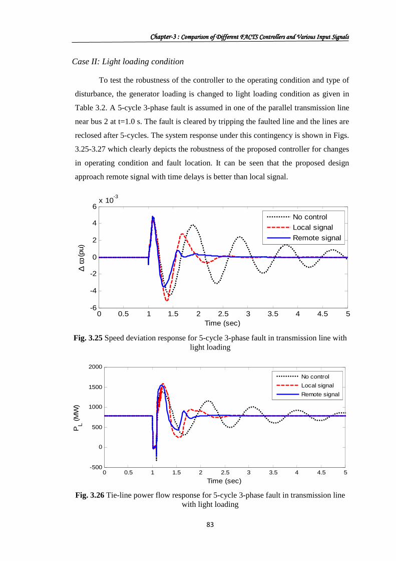
Case II: Light loading condition
To test the robustness of the controller to the operating condition and type of
disturbance, the generator loading is changed to light loading condition as given in
Table 3.2. A 5-cycle 3-phase fault is assumed in one of the parallel transmission line
near bus 2 at t=1.0 s. The fault is cleared by tripping the faulted line and the lines are
reclosed after 5-cycles. The system response under this contingency is shown in Figs.
3.25-3.27 which clearly depicts the robustness of the proposed controller for changes
in operating condition and fault location. It can be seen that the proposed design
approach remote signal with time delays is better than local signal.
0 0.5 1 1.5 2 2.5 3 3.5 4 4.5 5-6
-4
-2
0
2
4
6x 10
-3
Time (sec)
∆ ω
(pu)
No control
Local signal
Remote signal
Fig. 3.25 Speed deviation response for 5-cycle 3-phase fault in transmission line with
light loading
0 0.5 1 1.5 2 2.5 3 3.5 4 4.5 5-500
0
500
1000
1500
2000
Time (sec)
PL (
MW
)
No control
Local signal
Remote signal
Fig. 3.26 Tie-line power flow response for 5-cycle 3-phase fault in transmission line
with light loading

ChapterChapterChapterChapter----3 : 3 : 3 : 3 : Comparison Comparison Comparison Comparison oooof Difff Difff Difff Different FACTS Controllers erent FACTS Controllers erent FACTS Controllers erent FACTS Controllers aaaand Various Input Signalsnd Various Input Signalsnd Various Input Signalsnd Various Input Signals
84
0 0.5 1 1.5 2 2.5 3 3.5 4 4.5 5-0.2
-0.15
-0.1
-0.05
0
0.05
0.1
0.15
0.2
Time (sec)
Vq
(pu)
No control
Local signal
Remote signal
Fig. 3.27 Series injected voltage Vq for 5-cycle 3-phase fault in transmission line with light loading
Case III: Heavy loading condition
The robustness of the proposed controller is also verified at heavy loading
condition under small disturbance by disconnecting the load near bus 1 at t =1.0 s for
100 ms with generator loading being changed to heavy loading condition. The system
response under this contingency is shown in Figs 3.28-3.29 from which it is clear that
the system is unstable without control under this severe disturbance and the stability
of the system is maintained with the proposed GSA optimized SSSC-based damping
controller.
0 0.5 1 1.5 2 2.5 3 3.5 4 4.5 5-1
-0.5
0
0.5
1x 10
-3
Time (sec)
∆ω (
pu)
No control
Local signalRemote signal
Fig. 3.28 Speed deviation response for 5-cycle 3-ph fault in transmission line with heavy loading

ChapterChapterChapterChapter----3 : 3 : 3 : 3 : Comparison Comparison Comparison Comparison oooof Difff Difff Difff Different FACTS Controllers erent FACTS Controllers erent FACTS Controllers erent FACTS Controllers aaaand Various Input Signalsnd Various Input Signalsnd Various Input Signalsnd Various Input Signals
85
0 0.5 1 1.5 2 2.5 3 3.5 41400
1600
1800
2000
2200
Time (sec)
PL (
MW
)
No control
Local signal
Remote signal
Fig. 3.29 Tie-line power flow response for 5-cycle 3phase fault in transmission line with heavy loading
3.4.4 EFFECT OF SIGNAL TRANSMISSION DELAY To study the effect of variation in signal transmission delay on the
performance of controller, the transmission delay is varied and the response is shown
in Fig. 3.30. In this case, nominal loading condition with 5-cycle, 3-phase, self
clearing fault is assumed at the middle of one transmission line for the analysis
purpose. It is evident from Fig. 3.30 that the performances of the proposed controllers
are hardly affected by the signal transmission delays.
0 0.5 1 1.5 2 2.5 3 3.5 4-6
-4
-2
0
2
4
6x 10
-3
Time (sec)
∆ω (
pu)
Remote signal with 50 ms delay
Remote signal with 25 ms delay
Remote signal with 75 ms delay
Fig. 3.30 Speed deviation response showing for case of transmission delay

ChapterChapterChapterChapter----3 : 3 : 3 : 3 : Comparison Comparison Comparison Comparison oooof Difff Difff Difff Different FACTS Controllers erent FACTS Controllers erent FACTS Controllers erent FACTS Controllers aaaand Various Input Signalsnd Various Input Signalsnd Various Input Signalsnd Various Input Signals
86
3.5 EXTENSION TO MULTI-MACHINE POWER SYSTEM WITH SSSC
3.5.1 SYSTEM UNDER STUDY The proposed approach of designing and optimizing the parameters of a SSSC
based damping controller is further extended to a multi-machine power system shown
in Fig. 3.31. It is similar to the power system used in references [73, 74]. The system
consists of three generators divided in to two subsystems and are connected via an
intertie. Following a disturbance, the two subsystems swing against each other
resulting in instability. To improve the stability the line is sectionalized and a SSSC is
assumed on the mid-point of the tie line. The relevant data for the system are given in
Appendix III. For remote input signal speed deviation of generator G1 and G3 is
chosen as the control input of SSSC based damping controller and for local signal real
power flow at the nearest bus (bus5) is selected.
G2
G3
G1
T2
T3
BUS2
BUS1
BUS3
BUS4
BUS5 BUS6
LOAD1
LOAD2
LOAD3
T1
L2
L3
L1
L1
L1
L1
LOAD4
SSSC
Fig. 3.31 Three machine power system with SSSC
Two distinct types of system oscillations are usually recognized in
interconnected power systems [78]. One is associated with units at a generating
station swinging with respect to rest of the power system. Such oscillations are
referred to as local mode of oscillations and have a frequency in the range of 0.8 to
2.0 Hz. The term local is used because the oscillations are localized at one power
plant. The second is associated with swinging of many machines in one part of the
ChapterChapterChapterChapter----3 : 3 : 3 : 3 : Comparison Comparison Comparison Comparison oooof Difff Difff Difff Different FACTS Controllers erent FACTS Controllers erent FACTS Controllers erent FACTS Controllers aaaand Various Input Signalsnd Various Input Signalsnd Various Input Signalsnd Various Input Signals
87
system against machines in another part. These are inter area mode oscillations, and
have frequencies in the range of 0.2 to 0.7 Hz.
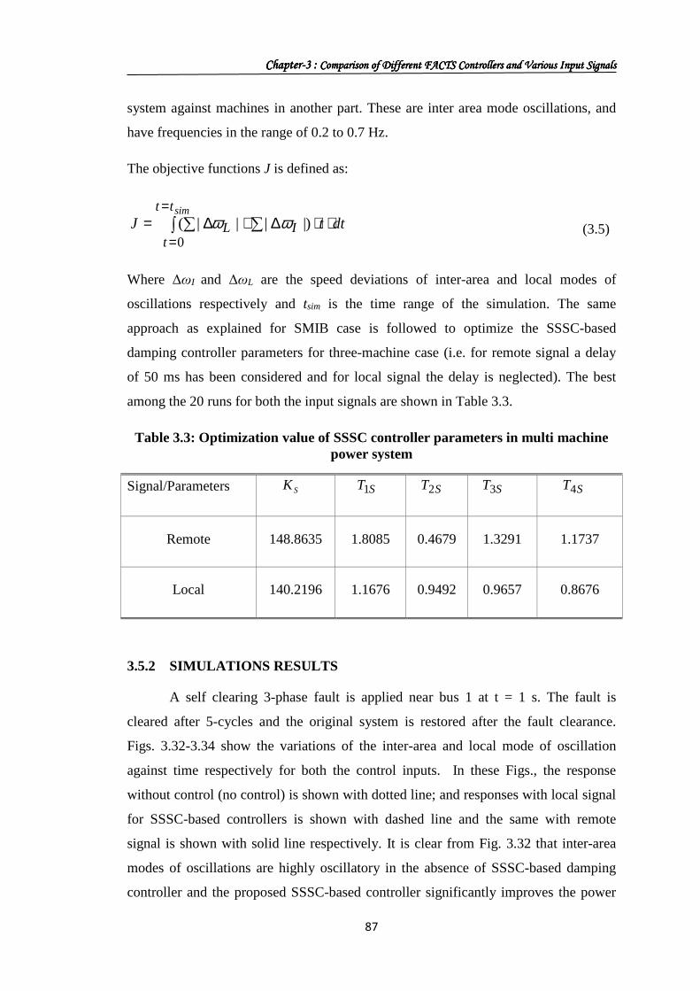
The objective functions J is defined as:
∫ ∑∑=
=⋅⋅∆+∆=
simtt
tIL dttJ
0)||||( ωω (3.5)
Where ∆ωI and ∆ωL are the speed deviations of inter-area and local modes of
oscillations respectively and tsim is the time range of the simulation. The same
approach as explained for SMIB case is followed to optimize the SSSC-based
damping controller parameters for three-machine case (i.e. for remote signal a delay
of 50 ms has been considered and for local signal the delay is neglected). The best
among the 20 runs for both the input signals are shown in Table 3.3.
Table 3.3: Optimization value of SSSC controller parameters in multi machine power system
Signal/Parameters SK ST1 ST2 ST3 ST4
Remote 148.8635 1.8085 0.4679 1.3291 1.1737
Local 140.2196 1.1676 0.9492 0.9657 0.8676
3.5.2 SIMULATIONS RESULTS
A self clearing 3-phase fault is applied near bus 1 at t = 1 s. The fault is
cleared after 5-cycles and the original system is restored after the fault clearance.
Figs. 3.32-3.34 show the variations of the inter-area and local mode of oscillation
against time respectively for both the control inputs. In these Figs., the response
without control (no control) is shown with dotted line; and responses with local signal
for SSSC-based controllers is shown with dashed line and the same with remote
signal is shown with solid line respectively. It is clear from Fig. 3.32 that inter-area
modes of oscillations are highly oscillatory in the absence of SSSC-based damping
controller and the proposed SSSC-based controller significantly improves the power
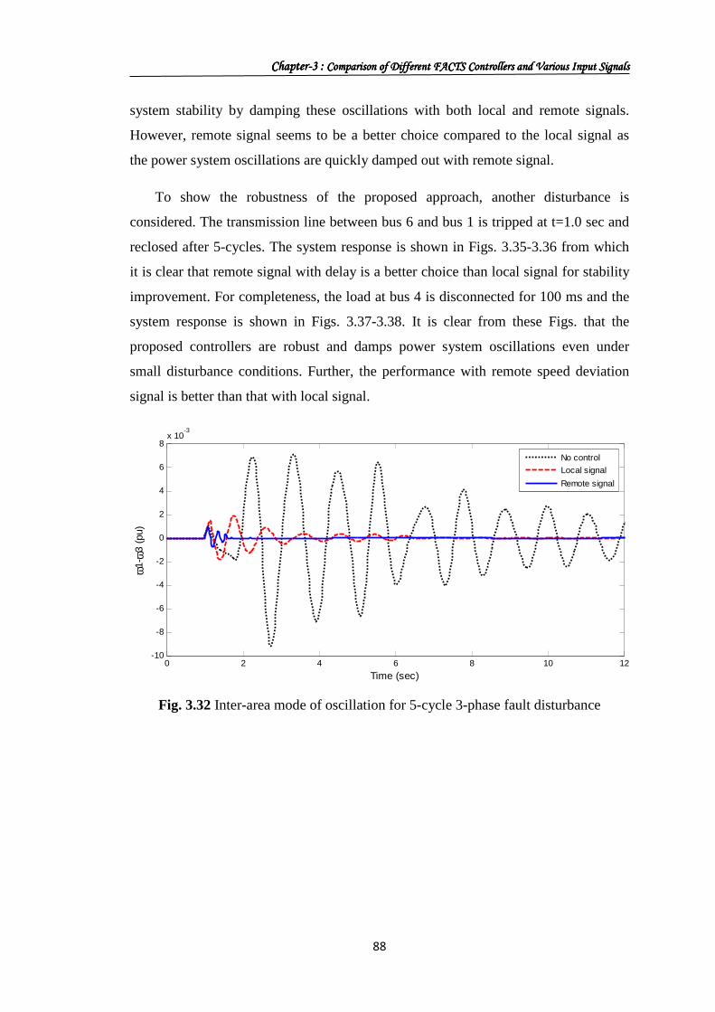
ChapterChapterChapterChapter----3 : 3 : 3 : 3 : Comparison Comparison Comparison Comparison oooof Difff Difff Difff Different FACTS Controllers erent FACTS Controllers erent FACTS Controllers erent FACTS Controllers aaaand Various Input Signalsnd Various Input Signalsnd Various Input Signalsnd Various Input Signals
88
system stability by damping these oscillations with both local and remote signals.
However, remote signal seems to be a better choice compared to the local signal as
the power system oscillations are quickly damped out with remote signal.
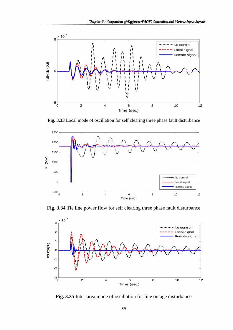
To show the robustness of the proposed approach, another disturbance is
considered. The transmission line between bus 6 and bus 1 is tripped at t=1.0 sec and
reclosed after 5-cycles. The system response is shown in Figs. 3.35-3.36 from which
it is clear that remote signal with delay is a better choice than local signal for stability
improvement. For completeness, the load at bus 4 is disconnected for 100 ms and the
system response is shown in Figs. 3.37-3.38. It is clear from these Figs. that the
proposed controllers are robust and damps power system oscillations even under
small disturbance conditions. Further, the performance with remote speed deviation
signal is better than that with local signal.
0 2 4 6 8 10 12-10
-8
-6
-4
-2
0
2
4
6
8x 10
-3
Time (sec)
ω1- ω
3 (p
u)
No control
Local signal
Remote signal
Fig. 3.32 Inter-area mode of oscillation for 5-cycle 3-phase fault disturbance
ChapterChapterChapterChapter----3 : 3 : 3 : 3 : Comparison Comparison Comparison Comparison oooof Difff Difff Difff Different FACTS Controllers erent FACTS Controllers erent FACTS Controllers erent FACTS Controllers aaaand Various Input Signalsnd Various Input Signalsnd Various Input Signalsnd Various Input Signals
89
0 2 4 6 8 10 12-5
0
5x 10
-3
Time (sec)
ω1- ω
2 (p
u)
No control
Local signal
Remote signal
Fig. 3.33 Local mode of oscillation for self clearing three phase fault disturbance
0 2 4 6 8 10 12-500
0
500
1000
1500
2000
2500
Time (sec)
PL (
MW
)
No control
Local signal
Remote signal
Fig. 3.34 Tie line power flow for self clearing three phase fault disturbance
0 2 4 6 8 10 12-3
-2
-1
0
1
2
3x 10
-3
Time (sec)
ω1- ω
3(pu
)
No control
Local signal
Remote signal
Fig. 3.35 Inter-area mode of oscillation for line outage disturbance

ChapterChapterChapterChapter----3 : 3 : 3 : 3 : Comparison Comparison Comparison Comparison oooof Difff Difff Difff Different FACTS Controllers erent FACTS Controllers erent FACTS Controllers erent FACTS Controllers aaaand Various Input Signalsnd Various Input Signalsnd Various Input Signalsnd Various Input Signals
90
0 2 4 6 8 10 12-3
-2
-1
0
1
2x 10
-3
Time (sec)
ω2- ω
3 (p
u)
No control
Local signal
Remote signal
Fig. 3.36 Local mode of oscillation for line outage disturbance
0 2 4 6 8 10 12-4
-2
0
2
4
6x 10
-4
Time (sec)
ω1- ω
3 (p
u)
No control
Local signal
Remote signal
Fig. 3.37 Inter-area mode of oscillation for small disturbance
0 2 4 6 8 10 12-2
-1
0
1
2x 10
-4
Time (sec)
ω1- ω
2 (p
u)
No control
Local signal
Remote signal
Fig. 3.38 Local mode of oscillation for small disturbance

ChapterChapterChapterChapter----3 : 3 : 3 : 3 : Comparison Comparison Comparison Comparison oooof Difff Difff Difff Different FACTS Controllers erent FACTS Controllers erent FACTS Controllers erent FACTS Controllers aaaand Various Input Signalsnd Various Input Signalsnd Various Input Signalsnd Various Input Signals
91
3.6 CONCLUSIONS
In this chapter, power system stability improvement by different FACTS
controllers namely SVC, STATCOM and SSSC based damping controllers is
thoroughly investigated. Both local and remote signals are considered. Speed
deviation of generator is taken as remote signal and line active power is taken as local
signal. For the controller design, appropriate time delays due to sensor time constant
and signal transmission delays are considered. The design problem is formulated as an
optimization problem and Gravitational Search Algorithm (GSA) is employed to
search for the optimal controller parameters. The performance of the proposed
controller is evaluated under different disturbances for both single-machine infinite
bus power system and multi-machine power system using both local and remote
signals. It is observed that STATCOM is slightly more effective than SVC from
stability point of view. It is also seen that best system response is obtained with SSSC
based damping controller. It is also noticed that the performance with remote speed
deviation signal is better than that with local signal for both single-machine infinite
bus power system and multi-machine power system.