comparison of measurement methods for partial discharge
TRANSCRIPT

1
Comparison of measurement methods
for partial discharge measurement in
power cables
L. W. van Veen
Supervisor: Prof. dr. J. J. Smit
Daily supervisor: Dr.ir. A. Rodrigo Mor
April 2014
INTELLIGENT ELECTRICAL POWER GRIDS

2

3
Nowadays it becomes more and more important to operate the electricity grid efficiently. To achieve
this, condition based maintenance is a good way to reduce maintenance time and costs. For
condition based maintenance partial discharge is an important tool to indicate insulation conditions.
This thesis focuses on partial discharge (PD) measurement in power cables. It focuses on ingnition of
PDs are triggered, what can be expected to measure, what kind of technologies are commercially
available for PD measurement and it compares PD measurement according to IEC60270
(conventional) with PD measurement not according to this standard (unconventional).
During ageing of a defect in a power cables, different PD mechanisms can occur. Aged defects have
lower generally inception voltage than virgin defects. PDs is measured by charge displacement in the
cable to the defect, that is related to the energy dissipated during a discharge and the volume of the
cavity.
During propagation of a PD pulse through a cable, high frequencies attenuate fast. Therefore their
amplitude decreases. Because the charge of the PD pulse does not attenuate in that large amount,
the pulse becomes wider. Furthermore the frequencies near DC attenuation more or less
proportional to the charge.
There are several types of PD measurement devices on the market, offline as well as online, all using
different voltage sources. Each voltage source has its advantages and disadvantages, depending on
applied stress, continuous duty, size, weight and max applied voltage.
Location is determined with Time Domain Reflectometry (TDR) or double sides measurement.
PDs measurement can be performed according to the standard (conventional measurement) or not
(unconventional measurement). There is a need for unconventional measurement because the time
response of conventional measurement is too long. There could occur overlap of pulse responses and
therefore it is not suitable for localization. This causes the need for unconventional measurement.
For conventional measurement there is a standard, for unconventional there is not. Therefore
manufacturers have developed systems with different sensors, that are not calibrated according to a
standard. Due to this, there can be differences in charge determination between systems.
Investigation of influence of the bandwidth of a system to the response of a PD, shows that filtering
frequencies have influence on time length of the response, the sensitivity of the system and the
charge determination.
Checking the accuracy of different charge determination methods for different sensors shows a wide
dispersion in accuracy. Determining charge by taking the peak value of the frequency spectrum
seems to be an accurate method for unconventional measurement. Depending on the pulses to be
measured, this method could be used with a wide range of sensors. Furthermore, the extension of
this method, that makes use of compensating the frequency spectrum of the measured PD, seems to
be also an accurate method.
Abstract

4
Because now there is also an accurate way to determine charge of PD pulses using different
sensors, unconventional measurements of different systems can be compared. Next to this,
unconventional measurement can be compared with conventional PD measurement.

5
Table of contents
Abstract ................................................................................................................................................... 3
Table of contents ..................................................................................................................................... 5
1 Introduction ..................................................................................................................................... 8
2 Partial discharges occurrence ....................................................................................................... 10
2.1 Introduction ........................................................................................................................... 10
2.2 PD mechanisms ..................................................................................................................... 10
2.2.1 Streamer ........................................................................................................................ 11
2.2.2 Townsend ...................................................................................................................... 11
2.2.3 Pitting ............................................................................................................................ 12
2.3 Types of PD ........................................................................................................................... 12
2.3.1 Internal discharges ........................................................................................................ 12
2.3.2 Surface discharge .......................................................................................................... 13
2.3.3 Corona ........................................................................................................................... 13
2.4 Properties of PDs that can be expected during PD measurement in cables ......................... 16
2.5 Initiation of PD activity .......................................................................................................... 16
3 Partial discharges representation ................................................................................................. 17
4 Propagation properties of PD pulses in power cables .................................................................. 20
4.1 Introduction ........................................................................................................................... 20
4.2 Pulse propagation properties ................................................................................................ 20
4.2.1 The telegraph equations ............................................................................................... 21
4.2.2 Attenuation and dispersion ........................................................................................... 23
4.2.3 Characteristic impedance and reflection of PD pulses .................................................. 26
4.2.4 Evaluation of a calibrator pulse through a MV cable .................................................... 27
4.3 Conclusion ............................................................................................................................. 31
5 Commercial available PD cable testing technologies .................................................................... 32
5.1 Introduction ........................................................................................................................... 32
5.2 Off-line measurement ........................................................................................................... 32
5.2.1 Introduction ................................................................................................................... 32
5.2.2 Sources for energizing the power cable during PD measurement ................................ 33
5.2.3 Resonant systems .......................................................................................................... 35
5.2.4 Damped AC voltage ....................................................................................................... 40
5.2.5 Sensors for offline measurement .................................................................................. 44
5.3 Localization of PD origin ........................................................................................................ 45

6
5.4 On-line measurements .......................................................................................................... 47
5.4.1 Introduction ................................................................................................................... 47
5.4.2 Principle ......................................................................................................................... 48
5.4.3 Equipment ..................................................................................................................... 49
5.5 Summary and conclusions ..................................................................................................... 51
6 Partial discharge measurements, conventional and unconventional ........................................... 53
6.1 Introduction ........................................................................................................................... 53
6.2 Conventional measurement .................................................................................................. 53
6.2.1 Introduction ................................................................................................................... 53
6.2.2 Standard ........................................................................................................................ 53
6.2.3 Description conventional PD measurement ................................................................. 54
6.2.4 Prescriptions of the IEC60270 standard for measuring PD ........................................... 55
6.2.5 Limits of the conventional measuring method ............................................................. 57
6.2.6 Feasibility conventional measurement method for PD measurement in MV cables ... 63
6.2.7 Conclusion ..................................................................................................................... 64
6.3 Unconventional measurements ............................................................................................ 64
6.3.1 Introduction ................................................................................................................... 64
6.3.2 Influence of the sensor on the PD pulse response. ....................................................... 65
6.3.3 Conclusion ..................................................................................................................... 71
6.4 Comparison of PD measurement methods ........................................................................... 72
6.4.1 Introduction ................................................................................................................... 72
6.4.2 Methods used for charge determination of PD pulses ................................................. 73
6.4.3 Simulations .................................................................................................................... 75
6.4.4 Conclusion ..................................................................................................................... 82
7 Influence of the measuring circuit on the measurements ............................................................ 83
7.1 Introduction ........................................................................................................................... 83
7.2 Influence of different measuring components on the gain of the system ........................... 83
7.3 Measurements ...................................................................................................................... 84
7.3.1 Coupling capacitor combined with measuring impedance ........................................... 84
7.3.2 High frequency current transformer ............................................................................. 87
7.4 Conclusion ............................................................................................................................. 88
8 Gain compensation of the measurement system ......................................................................... 89
8.1 Introduction ........................................................................................................................... 89
8.2 The method ........................................................................................................................... 89

7
8.2.1 Determination of the frequency response of the system ............................................. 90
8.2.2 PD signal compensation ................................................................................................ 90
8.2.3 Charge determination ................................................................................................... 91
8.3 Gain compensation in practice .............................................................................................. 91
8.3.1 Gain determination ....................................................................................................... 93
8.3.2 Gain compensation ........................................................................................................ 96
8.3.3 Applying gain compensation method to a high frequency current transformer .......... 99
8.3.4 Comparison of gain compensation method with determining charge by means of
taking the peak value of the frequency spectrum ...................................................................... 102
8.4 Conclusion ........................................................................................................................... 103
9 Summary and conclusions ........................................................................................................... 104
9.1 Conclusions and summary ................................................................................................... 104
9.2 Recommendations............................................................................................................... 106
A Appendix .......................................................................................................................................... 107
B Appendix .......................................................................................................................................... 110
C Appendix........................................................................................................................................... 112
Acknowledgements ............................................................................................................................. 113
Bibliography ......................................................................................................................................... 114

1 Introduction
8
Nowadays it becomes more and more important to operate the electricity grid efficiently, because
stakeholders, regulators and customers have high expectations of the electricity grid. Next to this, all
the assets deal with ageing. Transport and distribution service operators are trying to achieve a high
performance of the grid, in combination with a high reliability and a minimum of maintenance costs.
[23]
Possible maintenance methodologies to apply are:
No maintenance until breakdown (corrective maintenance)
Apply maintenance after constant periods of time (time based preventive maintenance)
Apply maintenance when the condition of the component is that bad that it will fail within a
short time (condition based preventive maintenance)
Breakdown of a cable without redundancy, leads to outage of the grid. This is not desirable;
corrective maintenance should better not be applied. It has shown that condition based maintenance
has advantages above time based maintenance, with its reduction in maintenance costs.[22] The
failure rate of assets behave like a the ‘bathtub curve’. The failure rate of an asset population in the
beginning of the lifetime is high because of manufacturing faults, during a long life time constant,
and at the end of the lifetime increased because of ageing.[14] To prevent failure of assets, it is
important to know the condition of the asset. After the component is installed in the grid, and after
ageing when the asset is in the last phase of its lifetime.
Through the years, it has been recognized that PD indicates danger to the life of insulation [14]. PD
measurement is one of the most important instruments to indicate insulation conditions.[3]
Nowadays there are several systems of different manufacturers to measure PD on the market. The
technical difference between systems can be found in the difference of the energizing sources, the
different sensors used, whether measured according to IEC60270, location determination and charge
determination. There are also practical considerations to choose a system; this has to do with weight,
size and duration of installation.
PD measurement can be performed according to the standard IEC60270, but this has some
limitations, especially for PD measurement in power cables. To overcome these shortcomings,
alternative systems have been developed: so called ‘’unconventional systems’’. For these systems,
there are no standards, what has lead to a wide range of varieties in systems.
1 Introduction

1 Introduction
9
PD measurement according to the standard, performs charge determination of PD pulses with low
uncertainty. For unconventional measurement there is no standard to be sure the charge is
measured correctly.
Because of the diversity in PD measurement systems with different sensors, there are a lot of factors
to consider when selecting a specific system. For example there could be made differences in charge
indication.
Before a power cable leaves the factory and after installing, the cable is tested for PD. When
measuring with different systems, it is important the measurements can be compared with each
other to get an unambiguous indication of the PD activity in the cable. This is also important in case
measuring a cable near the end of its life with different systems at different life times each, in order
to make an accurate PD activity evaluation in time.
The purpose of this Master thesis is to create the possibility to compare measurement results of
different PD measurement systems that are used for PD measurement in power cables.
The research objectives are:
Comparing different PD measurement techniques available on the market
Comparing conventional and unconventional measurement methods and show their
applicability to MV cable tests
Investigate different techniques for charge determination of PDs
Study the influence of the measuring circuit on PD measurement
This thesis gives in chapter 2 some information about different stages in ageing of insulation
materials. Chapter 3 gives a model of a cable with a defect, to give a practical idea of what happens
when a PD occurs. Chapter 4 gives some information about propagation of a PD pulse through a
cable and what can be expected to measure at the end of the cable.
Furthermore a comparison is made of different PD measurement systems available on the market in
chapter 5. Chapter 6 compares conventional and unconventional measurement with respect to PD
measurement in power cable. The opportunities and limitations are investigated to come to a
conclusion about their applicability. Chapter 7 treats the influence of the measuring circuit on the PD
measurement. In chapter 8 is investigated a universal method to determine charge in an accurate
way using unconventional measurement.

2 Partial discharges occurrence
10
2.1 Introduction The definition of a partial discharge according to IEC60270 is: Localized electrical discharge that only partially bridges the insulation between conductors and which can or cannot occur adjacent to a conductor.
Partial discharges are in general a consequence of local electrical stress concentrations in the insulation or on the surface of the insulation. Generally, such discharges appear as pulses having a
duration of much less than 1 s More continuous forms can, however, occur, such as the so-called pulse-less discharges in gaseous dielectrics. This kind of discharge will normally not be detected by the measurement methods described in this standard. Partial discharges are often accompanied by emission of sound, light, heat, and chemical reactions. A PD causes a PD pulse. This is a current or a voltage pulse that results from the PD, caused by the displacement of charge. PDs occur most likely in gas, vapour or in low density regions in oil. They are indicators for defects in
the insulation materials. They degradate the insulation material as well as the electrode, and sooner
or later the insulation will break down.
There are three conditions for the generation of PDs:
1 A starting electron must be available
2 An avalanche is created by ionization
3 A feedback mechanism has to be present
[12]
Before a PD can take place, a starting electron must be present. This electron can be released from
the electrode or from the gas in which the discharge will take place. Furthermore the field strength
must be sufficiently high for the electron to gain enough kinetic energy to cause an avalanche by
ionization. This created avalanche has to maintain itself, therefore a feedback mechanism has to be
present.
2.2 PD mechanisms Three common PD mechanisms that can cause a partial discharge are:
1 Streamer mechanism
2 Townsend mechanism
3 Pitting
2 Partial discharges occurrence

2 Partial discharges occurrence
11
During the ageing process they occur in the above ranked way.
2.2.1 Streamer
A streamer is formed when an avalanche reaches the critical number of 10^8 charge carriers. At this
value there is generated extra ionization. This extra ionization and thereby the generation of extra
photons take care for the feedback mechanism, let the avalanche further grow and make new
avalanches that grow to each other. Therefore the avalanche can maintain itself and a streamer is
formed.
The breakdown channels of a streamer are narrow and the discharge time is relative short (about 1-
10ns) [14]. During streamer discharge, only small part of the surface participates to a discharge,
other small parts discharge individually. This can occur very fast and the pulses tend to overlap [12].
2.2.2 Townsend
Townsend occurs only in cavities where the condition of the size of the cavity and the pressure in the
cavity exceed the Paschen’s curve (see figure 2.1). This curve gives the condition for the voltage and
the pressure * size of the cavity to initiate a discharge in the cavity. Townsend in general works until
(pressure * distance) is 5bar*mm.
Figure 2.1: Paschen’s curve [13]
When the conditions for the Townsend mechanism are fulfilled, a starting electron can create an
avalanche by ionization. Some photons and the formed ions move to the cathode. When they hit the
cathode, there is a probability that a new starting electron is initiated, which causes a new avalanche.
This is how the feedback mechanism of Townsend works. So the feedback for the Townsend
mechanism depends on the cathode material. The discharge process is shown in figure 2.2. The
Townsend mechanism causes a diffuse discharge, a large area of the cavity surface participates
within the discharge. For cavity depths of 0.1 to 1mm the discharge duration takes respectively about
80ns – 0.8s [14]. This is caused by the slowly moving ions that can create new starting electrons
when they reach the cathod. Because the charge displacement is the same as in the streamer stage
but the discharge time is longer, the pulse has lower amplitude.

2 Partial discharges occurrence
12
Figure 2.2: Townsend discharge process
2.2.3 Pitting
As a cause of ageing of the cavity wall by repetitively discharges in the cavity, pitting may occur under
AC voltage. During discharging, by-products are produced. After a long time of discharging, the
concentration of by-products is so large that there is going to form a conductive layer of crystals at
the cavity wall. When the crystals are formed, there is generated field enhancement at the sharp
edges of the crystals. At these edges, discharges occur far earlier than in the other stages of the
material. The discharges take place in smaller space and have a low magnitude in combination with a
relative high repetition rate. Due to the low magnitude (0.2pC) and the high repetition rate Pitting is
much harder to measure.
2.3 Types of PD PD’s can be harmful for the dielectric of cables.[14].
There are three types of partial discharges:
Internal discharges
Surface discharges
Corona discharges
2.3.1 Internal discharges
Internal discharges can occur in cavities that are present in solid insulation. They are also formed by
the electrical treeing process, that wears out a cavity in the insulation. There can be made a
distinction between cavities that are electrode bounded or totally enclosed by insulation material.

2 Partial discharges occurrence
13
Causes of PD’s in solid dielectrics are shown in figure 2.3
Figure 2.3: Internal discharges in solid dielectrics [14]
Ageing process
Virgin cavities
Unaged cavities, totally enclosed by dielectric material, do not have a conductive cavity wall.
Therefore Townsend is not possible to occur in the so called ‘virgin cavities’. In that case the voltage
must increase to about 5% higher than required following the Paschen’s curve for creating the
required condition of streamers.
Aged cavity
After some time streamer discharges occurrence, there is formed a conductive layer on the cavity’s
surface. This is caused by chemical changes of the surface, formed during the discharges. Now the
surface of the cavity is conductive, the Townsend mechanism can take place.
During the latest stage large discharges that start from the edge of the cavity occurs that appears in
intermittent way. They seem to have a relation to breakdown and are a sign of progressive ageing.
2.3.2 Surface discharge
Surface discharges are streamer discharges that could initiate at a high tangential field strength along
the interface. When PDs are detected near their inception voltage, is shows no difference between
surface and internal PD. In case the voltage applied is raised, the discharge occurs along a longer
surface. Thereby the surface discharge increases in length and magnitude. In this way surface
discharge is easily to distinguish from internal discharges.
2.3.3 Corona
Corona occurs around sharp points in a high electric field. During PD measurement in cables, sharp
edges at the end terminations can cause corona and could be covered with metallic round caps to
bring the surrounding of the sharp point at equal potential. Corona can mask detection of other
discharges during PD measurement. There are two types of corona: positive and negative corona.

2 Partial discharges occurrence
14
Negative corona
Negative corona occurs at negative voltage. Figure 2.4 shows a point at negative voltage, in the
vicinity of a cathode. Townsend discharges take place and the formed electrons of the ionization are
at larger distance attached to an electronegative gas (Oxygen in Air). In this way heavy negative ions
are formed. These ions are too heavy and slow to participate in the creation of avalanches and form
a cloud in front of the negative electrode. Because presence of a cloud of negative heavy ions, the
field strength is decreased and the discharges are stopped. When the space charge cloud of heavy
ions has moved away, the discharge are initiated again. The electronegative gas is required for this
recurrent appearing discharges. Negative corona occurs in case the voltage is sufficient to release
electron out of the electrode, discharge peaks are measured symmetrical around the negative
voltage peak of the sinusoidal AC voltage waveform. The magnitude of the discharges is constant, but
the repetition rate increases with the voltage.
Figure 2.4 : Negative corona [13]
Positive corona
Positive corona has a higher inception voltage than negative corona. During positive corona, there is
absence of a cathode at the high field strength. Streamers are formed in the gas, near the sharp point
with high field strength, and cause the presence of positive ions in front of the sharp point (see figure
2.5). These positive ions form a positive space charge and let the field strength at the electrode
decrease. At a certain field strength, the generation of streamers extinguishes. After the space
charge of heavy ions is drifted away, generation of streamers is initiated again. The pattern of
positive corona is not as regular as with negative corona and at higher voltages, large streamers can
be generated.
Figure 2.6 shows the occurrence of PD along the phase angle of the applied voltage. It also shows
that negative corona has a lower inception voltage than positive corona.

2 Partial discharges occurrence
15
Figure 2.5 : Positive corona [13]
Figure 2.6: a) Negative corona after voltage rise b) Positive and negative corona after voltage rise
[13]

2 Partial discharges occurrence
16
2.4 Properties of PDs that can be expected during PD measurement in
cables The shape of a PD pulse depends on the propagation path of the pulse before it is measured. PDs
with origin at or near the point of measuring have almost their original shape. In MV cables, the high
frequency content of a pulse attenuates very fast. The longer the propagation path of the pulse, the
more high frequency content is lost and the wider the pulse. Chapter 4 goes more in detail into this
process.
2.5 Initiation of PD activity PDs are initiated at a certain voltage, the extinction voltage Vi. The definition according to IEC60270 is: applied voltage at which repetitive partial discharges are first observed in the test object, when the voltage applied to the object is gradually increased from a lower value at which no partial discharges are observed. In practice, the inception voltage Vi, is the lowest applied voltage at which the magnitude of a PD pulse quantity becomes equal to or exceeds a specified low value.[9] When a PD is initiated, it usually continues at this voltage, but usually also when the voltage is
decreased a bit. The PD activity extinguishes at a certain voltage level, equal or below the inception
voltage. This is called the extinction voltage. IEC60270 describes it as: applied voltage at which
repetitive partial discharges cease to occur in the test object, when the voltage applied to the object
is gradually decreased from a higher value at which PD pulse quantities are observed. In practice, the
extinction voltage Ve is the lowest applied voltage at which the magnitude of a chosen PD pulse
quantity becomes equal to, or less than, a specified low value.[9]
Defects with Vi smaller than the operating voltage, produce PD when the cable is energized. This PD
activity will continue during operation. Because the PD damages continuously the cable insulation, it
brings a high risk on failure of the cable.
Another situation is Vi > operating voltage, but Ve < operating voltage. In this case, the PD is
triggered by a peak voltage caused by for example lightning or switching. When the PD activity is
initiated, there is a chance the PD activity maintains during operation. It can also disappear for some
time and show up after a while, or the activity can extinguish in total. This kind of defects will be
found during PD measurement when a higher voltage than the operating voltage is applied. In case
of online measurement, only when already a surge has caused the PD initiation.
The last case is Vi > operating voltage and Ve > operating voltage. During operation these PDs can be
initiated when transient overvoltages occur and extinguish fast after couple of cycles of the operating
frequency. Commonly these PDs are not harmful, but there is a probability that this PD activity can
cause a tree in the insulation material that could maintain below operating voltage because of high
electric field at the tips of trees. [11]

3 Partial discharges representation
17
Due to the fact that partial discharges are related to ageing of a cable, charge measurement of PDs is
usefull. When a cable sample has an internal defect or a surface defect, a practical scheme can give a
representation of the situation, like depicted in figure 3.1
Figure 3.1: equivalent circuit for internal and surface discharges [14]
a) Represents the sound part of insulation b) Represents dielectric in series with the gaseous capacitance c c) Represents a cavity or part of the surface that flashes over
Because there cannot be measured over the defect itself, we have to measure the charge displacement in the conductors to the sample. This is often done by putting a measuring impedance into the electric circuit to the sample. The measured charge is not the real charge displacement, the external charge displacement is measured. (3.1) The real charge displacement in the defect is: (3.2)
Where V is the V of figure 3.2. Because in general capacitance b << capacitance c, the PD pulse magnitude measured is far smaller than the real magnitude. The relation between the measured magnitude and the real magnitude is unknown, but there are two reasons why this method is used.
3 Partial discharges representation

3 Partial discharges representation
18
The first reason is that the measured discharge magnitude in combination with the inception voltage can be related with a reasonable approximation to the energy dissipated during a discharge. For the derivation of this relation we use the model of figure 3.2.
Figure 3.2: Model with components playing a role in charge displacement during PD [14] a Represents the sound part of insulation b Represents dielectric in series with the gaseous capacitance c c Represents a cavity or part of the surface that flashes over Vi Represents the instantaneous PD inception voltage of the cavity U Represents the voltage across the cavity before a discharge of c
V Represents the voltage drop over c caused by a discharge
When PD occurs, some charge is displaced from capacitor c to b. The following points gives information over the voltage over b and c and the displaced charge.
When a discharge occurs, the voltage across c drops with V
Due to that, the voltage across b increases with V and the voltage over c becomes V
The charge displacement to b is given by
The energy dissipated during a discharge can be related to the charge in the following way:
Before discharge, the energy stored at c is
After discharge, the energy stored at c is
The dissipated energy becomes
(3.3)
Now we are making an error in order of 10% by taking Because usually b<<c
(3.4)

3 Partial discharges representation
19
Making the assumption b<<c compensates more or less the error of (U+V)=U. The dissipated energy becomes:
Cables with the same nominal voltage have about the same inception voltage and the same discharge magnitudes are comparable. [14] The measured charge is also related to the volume of the discharge. Figure 3.3 gives a representation of dimension parameters of a piece insulation material with a dischargeing cavity. Now we use figure 3.3 and derive the relationship between the volume of the discharge area and the measured charge displacement q.
When V increases with L, and q increases with SV, q rises with the volume of the discharge.
Figure 3.3: Dimension parameters of a piece insulation material with a dischargeing cavity [14]
Because q is related to the energy dissipated during a discharge and the volume of the discharge area, it is a good measure for PD.

4 Propagation properties of PD pulses in power cables
20
4.1 Introduction When a PD pulse propagates trough a coaxial MV cable, the PD pulse changes of shape, caused by
attenuation and dispersion. Non destructive electrical PD measurements in cables is always
performed at the end of the cable. PD pulses in MV cables often have to travel a significant distance
before arriving at the measuring system. For PD measurement in cables, it is useful to have an idea
what happens with a PD pulse that propagates through the cable. Therefore this chapter gives an
insight about what happens with the PD signal during propagation through the cable and what
happens with the pulse at the end of the cable.
4.2 Pulse propagation properties A cable can be modelled by a circuit of many sections of inductors in series, with between each
inductor section a capacitance in parallel. A model is shown in figure 4.1
Lz Lz Lz
zz-z z+z
Cz Cz Cz
V(z)
I(z)
Figure 4.1: A simple model a MV cable
After closing the switch in figure 4.1 it takes a while before the voltage arrives at the other side of the
cable. The applied voltage causes a current through the first inductor and this current charges the
first capacitance. When the capacitances get charged, the voltage rises and causes a current through
the next inductor that charges the next capacitance. This process takes some time.
The current through the cable is equal to the differential of the charge with respect to the time:
(4.1)
The voltage induced between the conductor and earth screen at t0 and x0 is:
(4.2)
4 Propagation properties of PD pulses in power cables

4 Propagation properties of PD pulses in power cables
21
We know that the induced voltage at t0 and x0 equals the source voltage. Therefore the travelling
speed has to be equal to:
(4.3)
So when a PD pulse is injected in a cable, the travelling velocity of the pulse is equal to equation 4.3.
Equations that describe propagation of electrical signals through the coaxial cable are the telegraph
equations. These are treated in chapter 4.2.1.
4.2.1 The telegraph equations
The propagation of pulses through a cable is described by the telegraph equations. To get a more
realistic model of a MV cable, the model of figure 4.1 is modified. During propagating through a
cable, attenuation of the pulse signal arises, caused by the resistivity of the conductor and by leakage
between the two conductors. Figure 4.2 gives a model for this. The ohmic losses dissipated in the
conductor are represented by resistor R [m] and the leakage current is caused by conductance
G[Sm]. The figure gives a representation an infinitely small lines section z.
L R
C G
Figure 4.2: Model of a MV cable section with loss factors
Now we are going to have a look at the Telegraph equations to get insight of the behaviour of the
pulse during propagation. For deriving the telegraph equations, Kirchhoff’s laws are used in
combination with the model of figure 4.2.
(4.4)
(4.5)
(4.6)
(4.7)
(4.8)

4 Propagation properties of PD pulses in power cables
22
(4.9)
Where
L [H/m]
R [/m] C [F/m ] G [Siemens/m]
The minus sign for decreasing of i(z,t) and u(z,t) during propagation in positive direction. To solve
these equations 4.6 and 4.9, Laplace is needed. We go from the time domain to the frequency
domain and we take
.
(4.10)
(4.11)
(4.12)
(4.13)
(4.14)
(4.15)
(4.16)
When taking for p = j, propagation coefficient becomes like equation 4.17.
(4.17)
When the losses are small can be approximated by equation 4.16.
(4.18)
(4.19)
(4.20)
And the velocity of the pulse is equal to equation 4.21.
(4.21)
Equation 4.19 shows that the attenuation constant is independent of frequency. The same is
displayed in equation 4.21 for the phase velocity. This means that the signal shape does not change
during propagation and that the cable is distortionless.

4 Propagation properties of PD pulses in power cables
23
In real, the attenuation constant for PD pulses in a cable is not independent of frequency. Some
frequencies will attenuate more during propagation than others; especially high frequencies face
large attenuation in MV cables. Next to attenuation, there occurs dispersion. In the next subchapter
there is treated attenuation and dispersion using the model of figure 4.5 and there is shown some
information about frequency related attenuation and dispersion.
4.2.2 Attenuation and dispersion
As already discussed in the previous chapter, during propagation of a pulse through a cable, there
occurs attenuation and distortion. Distortion causes change in pulse shape, but also attenuation
causes this. Figure 4.3 shows measured reflections of a calibrator pulse travelling through a MV
cable. The pulse is reflected against very large characteristic impedance, therefore it is fully reflected
at the ends of the cable. It shows that the pulse shape changes a lot during propagation.
Figure 4.3: Reflections of a calibrator pulse travelling through a cable.
To analyse the cause of distortion and attenuation, we consider a little more advanced model than
used before. Figure 4.4 shows the cross-section of a XLPE cable. From inside to outside there is
depicted the aluminium conductor, the inner semiconductor the XLPE insulation, the outer
semiconductor screen, the outer-outer semiconductor screen, the copper conductors and the PVC
sheath. This cable is modelled by figure 4.5, where the semiconductor layers are shown as the
conductor shield and ground shield. We take this model into account for further analysis.

4 Propagation properties of PD pulses in power cables
24
Figure 4.4: Cross-section of a MV cable
Figure 4.5: Model of a MV cable section depicted in figure 4.4 [27]
Attenuation of the PD pulse can be caused by conductor losses as skin effect, but also by losses in the
insulation material
As we look at the total losses in a MV cable, models and measurements in [16] show that the
frequencies above 100kHz are far more attenuated than below. These results are depicted in figure
4.6.
Figure 4.6: Attenuation of an XLPE cable [16]

4 Propagation properties of PD pulses in power cables
25
References [16] shows that the attenuation in XLPE cables of the frequency range below 10MHz is
mainly caused by losses in conductors as skin effect, figure 4.7. This attenuation rises with the square
root of the frequency. The higher frequency attenuation is mainly caused by the dielectric system.
Reference [27] shows that for PILC cables the attenuation of the frequency range below 1MHz is
mainly caused by the skin effect. Paper insulated cables have a much larger tan [14] than XLPE
cables. Figure 4.7 shows the contributions of attenuation caused by conductor losses and dielectric
losses of an XLPE cable.
Figure 4.7: Attenuation contribution of dielectric and conductor of an XLPE cable [16]
Dispersion is caused by the difference between the group velocity of all the frequencies of the pulse
and the phase velocity of each frequency. The propagation velocity is approximated by
. The
variation of the capacitance between the conductor and the copper sheath takes care for almost the
entire dispersion below 100MHz. The little inductance variation caused by the skin effect has only a
small effect.[20] With increasing frequency, the semiconductor layers transform from ohmic to
capacitive. This leads to a total capacitance between conductor and ground that is decreasing with
frequency. As a consequence of this, the velocity for higher frequencies increases with frequency.
This different velocities cause phase shift in the frequency spectrum during propagation. Therefore
the pulse is distorted and the shape in the time domain is modified. [20]
When the electric and magnetic field distribution between the conductor and the neutral conductor
are analysed, based on the semiconductor properties, it is shown that variation in velocity over the
frequency spectrum occurs in the region the semi-conducting layers changes from resistive stage to
the capacitive stage. Outside this region the velocity is nearly constant, but different in the high
frequency region and in the low one. Therefore dispersion has only a significant influence in the
regions of two decades of frequency with the centre frequency of equation 4.22

4 Propagation properties of PD pulses in power cables
26
(4.22)
With
The conductivity of the semiconducting layer as a function of frequency
The permittivity of the semiconducting layer as a function of frequency
In reference [19] there is given a realistic example of dispersion in an XLPE cable. It is shown that
dispersion occurs in the MHz regions.
A question that rises is what happens in the time domain with a pulse that is influenced by
attenuation and distortion and what is the amount of these two factors in practice.
Reference [20] shows that dispersion causes a shorter rise time than fall time of a PD pulse, the pulse
is made more asymmetric. Attenuation causes the strong decrease in amplitude. Where dispersion
causes more asymmetry in the pulse, attenuation of high frequencies cause a decrease in amplitude,
and therefore a widening of the pulse.
This attenuation causes an increase of rise time that is larger than the fall time is increased by
dispersion. The high frequency energy is spread in time as a result of dispersion [20], but this has not
a significant influence on the amplitude of the pulse that is decreased by attenuation.
In short, the strong attenuation of high frequencies neglects the influence of dispersion on a PD pulse. Therefore the pulse becomes more symmetric. Measuring differences between arrival times by counting difference in peak times become less accurate. This has negative consequences for localization. [20] In chapter 4.2.4 there is done an experiment to check how a calibrator pulse evolutes over travelled
distance. But first, the next chapter gives some basic information about the characteristic impedance
that can be useful for measuring PD.
4.2.3 Characteristic impedance and reflection of PD pulses
The relation between voltage and current of a pulse, for every infinite small point of the cable is
determined by the per section capacitance and inductance of the cable. This relationship between
voltage and current at a single point in the cable is called the characteristic impedance.
When using the model of figure 4.1 and equation 4.1 and we substitute the velocity v by equation
4.3, equation 4.23 is obtained and gives the characteristic impedance.
(4.23)
This corresponds to a distortionless lossless line that is not a real case, but to explain the basics of
pulse propagation, this model is very useful. For PD measurement in cables, it is important to know
something about the characteristic impedance. During propagation of a PD pulse in a cable, it faces a
constant environment, the characteristic impedance is constant. But in case the PD pulse reaches a
joint, the propagation environment shows differences with the Zc of the cable. The capacitance and
inductance differ and therefore the relation between voltage and current will differ also. In case an
end termination is reached, the characteristic impedance is even zero (in case of short circuited

4 Propagation properties of PD pulses in power cables
27
termination) or infinite (open end termination). Short circuited terminations are not used in high
voltage measurements.
When the PD pulse travels in forward direction and reaches a different medium, the characteristic
impedance changes and the relation between voltage and current becomes different. A piece of the
pulse is reflected into the backward direction and a piece is transmitted in the forward direction. The
pulse is split in two parts. When two cables with different characteristic impedances are connected,
voltage and current are continuous at the interface. Because there is reflected a part of the pulse,
there can be made the conclusion that the reflected pulse plus the incoming pulse is equal to the
transmitted pulse.
The voltage waves are described by:
(4.24)
The current waves are described by:
(4.25)
(4.26)
(4.27)
When a PD pulse arrives at the open end of a cable, Z2 is infinite. When measurement is performed
at the end of the cable, Vr(x,t) = Vi(x,t) and there is measured the incoming and reflected voltage at
the end termination. Therefore the measured voltage is twice the incoming voltage.
After generation of a PD, half of the charge travels to one half of the cable and the other half travels
to the other side. Half of the pulse charge is arriving at the end of the cable, but there is measured
the correct signal because of the voltage doubling at the very high measuring impedance at the end
of the cable.
In case calibrating at the measurement side, the first pulse is measured at correct amplitude. When
system calibration is performed at the opposite open end of the cable, the injected pulse travels to
the measuring system with a very high impedance and there is measured twice the original incoming
signal. This has to be taken into account.
Furthermore when a cable is measured with one or more joints, there can be measured reflections of
PD signals that are reflected against joints.
4.2.4 Evaluation of a calibrator pulse through a MV cable
Now we are going to evaluate the frequency spectrum of a calibrator pulse propagating through a
cable, the pulse sequence 506 of appendix C. The pulse is injected at one side of the MV cable. At the
opposite side, the reflections are measured. There are measured 4 reflections, with travelled
distances starting at 640m and with an addition of 1280m for every reflection.

4 Propagation properties of PD pulses in power cables
28
The time domain records and the cumulative charge are plotted in figure 4.8. It is shown that the
amplitude of the pulse decreases fast, while the charge is not decreasing that fast. The pulse
becomes wider, therefore the charge, that is proportional to the area beneath the pulse, is not
attenuating as much as the amplitude.
By evaluation of the frequency spectrum of the pulse that propagates through the cable, the cause of
the rapidly decrease of the pulse amplitude can be discovered. The frequency spectrum of the
recorded pulses is calculated by the FFT function in Matlab, the results are shown in figure 4.9.
Figure 4.9 shows that the high frequencies attenuate very fast. This causes the fast decrease in
amplitude of the time signal of the pulse. When making a link to PD measurement, it can
Figure 4.8: Measured different reflections of calibrator pulse and their integral
be said that using a band pass filter with a low high cutoff frequency, looses sensitivity. This is the
case especially for smaller pulses that have left a significant high frequency content. In chapter 6 it is
investigated the influence of the cutoff frequencies on the pulse in time domain.
For measurement of PD pulses that have travelled some km through a cable, is it is probably less
useful to use a system with a high low cutoff frequency of some hundreds of kHz, because there is
probably filtered away a lot of information.
This chapter gives an insight of the properties of a PD pulse after travelling through a cable. It gives
an idea of the frequency range that can be measured. More information about the influence of filters
on the PD pulse is shown in chapter 6.

4 Propagation properties of PD pulses in power cables
29
Figure 4.9 shows that the high frequency content is attenuated much more than the frequencies of
about below 100kHz. When zoomed in a little more, the cable seems to behave like a low pass filter.
It displays that the frequency spectrum below about 40kHz is staying flat, these frequencies seem to
attenuate with the same factor during propagation of the pulse through the cable.
Because the charge is not attenuated as much as the amplitude of the pulse and the fact that the low
frequency regions attenuate also not that much during propagation, rises some interest in
investigation whether there is a relation between the charge and the low frequencies of the pulse.
The charge of the pulse obtained with the measured voltage signal is:
(4.27)
Where X[n]= a sample with index n of the measured voltage signal T = time between two samples = 1/sample rate Zc is the characteristic impedance of the cable
When calculating the frequency spectrum of the measured signal, the discrete the Fast Fourier
Transform is used. This frequency spectrum will be:
The calculation of the frequency spectrum value for =0, corresponds always to the first calculated
value of the spectrum. In this case it corresponds to X[1] in equation 4.28. When calculating this
value, equation 4.29 results.
When scaling this by the factor
, equation 4.30 is obtained.
This is the same as equation 4.27 and therefore, the charge is obtained with the DC value of the
frequency spectrum.
Figure 4.10 shows the frequency responses, scaled by factor
, and the cumulative charge of pulse
set 506 of appendix C. As displayed, the DC value of the frequency spectrum equals the highest value
of the cumulative charge. Also the lower frequencies, close to the DC value have about the same
magnitude. Therefore it can be said that they attenuate more or less with the charge. In chapter 6.4
there is written more about this topic.

4 Propagation properties of PD pulses in power cables
30
Figure 4.9: Frequency spectrum of recorded pulses of figure 4.7
Figure 4.10: Frequency spectrum and cumulative charge of pulse set 506 of appendix C
0 2 4 6 8 100
5
10
15
20
25
30
MHz
mV
Freq. resp. cal. pulse travelled different distances
640m travelled
1920m travelled
3200m travelled
4480m travelled
0 0.2 0.4 0.6 0.8 15
10
15
20
25
30
MHzm
V
Freq. resp. cal. pulse travelled different distances zoomed in
640m travelled
1920m travelled
3200m travelled
4480m travelled
0 0.2 0.4 0.6 0.8 1 1.2 1.4 1.6 1.8 20
50
100
150
200
250
300
350
400
450
MHz
mV
Freq. spec. reflection 1
Freq. spec. reflection 2
Freq. spec. reflection 3
Freq. spec. reflection 4
0 500 1000 1500 2000 2500 3000 3500
0
50
100
150
200
250
300
350
400
450
ns
pC
Frequency spectrum and cumulative charge of pulse set 506 of appendix C
Cumulative charge reflection 1
Cumulative charge reflection 2
Cumulative charge reflection 3
Cumulative charge reflection 4

4 Propagation properties of PD pulses in power cables
31
4.3 Conclusion During propagation the shape and the amplitude of a PD pulse change. Knowledge about these
changing properties, this could helps to select a useful sensor for a PD measuring system.
When a PD pulse travels through a MV cable, attenuation and dispersion occur. Attenuation causes a
decrease of the amplitude of the pulse. Dispersion causes an asymmetry in the shape of the pulse.
This causes the smaller rise time than fall time.
Dispersion occurs in the MHz regions. In practice, the high frequency content of a PD pulse travelling
through a MV cable is attenuated relatively fast. Next to the rapidly decreasing amplitude, the pulse
becomes wider in time. Because the MHz frequency regions attenuate rapidly, dispersion plays only a
very little role in the shape change of the pulse.
During an experiment with a calibrator pulse in a real MV cable, it turned out that indeed the high
frequencies attenuate very fast. This causes a fast decrease in amplitude of the pulse. Therefore
measuring, especially steep PD pulses, with a band pass sensor with a low high cutoff frequency
decreases the sensitivity a lot.
Usage of a system with a high low cutoff frequency causes measurement losses of usefull
information about the PD pulse. Therefore these systems are not recommended.
When looking at frequency spectrum of a PD pulse travelling through a MV cable, the lower
frequencies of tens of kHz attenuate much lesser than the higher frequencies. The cable seems to act
like a low pass filter. The lower frequencies seem to attenuate proportional with the integral of an
UWB pulse, so proportional to the charge. The value proportional to the charge of a pulse can be
derived from the DC value of the frequency spectrum. Frequencies close to the DC frequency, have
about the same magnitude as the frequency spectrum magnitude at DC. Therefore it can be said that
the lower frequencies attenuated more of less proportional to the charge.

5 Commercial available PD cable testing technologies
32
5.1 Introduction In this chapter available PD testing technologies are presented and studied. For the measurement of
partial discharges there is a standard specified, IEC60270. So measurements can be performed
according to this standard (conventional measurement) or not (unconventional measurement). Next
to this, the distinction can be made between PD measurement when the cable is in operation (online
measurement) and PD measurement when the cable is offline (offline measurement). Also there are
different sources to energize the test object. Finals a distinction between used sensors and PD
localization methods is made. First offline measurement is considered and afterwards online
measurement.
5.2 Off-line measurement
5.2.1 Introduction
Offline measurement of PDs requires an uncoupled and de-energized power cable, an external
power supply and a measuring circuit. Several kinds of voltage signals can be applied to energize the
cable. The selection of a source depends on several parameters. It makes a real difference if you are
measuring in the field or in the laboratory. While measuring in a laboratory has almost no
restrictions, measuring in the field is more complex. In the field power requirements play a large role.
Also weight, size and time to install of the measurement system play a role.
Cables’ capacitance increase with the length of the cable. When 50Hz voltage is applied to energize a
long cable, the large capacitance of the cable requires a large reactive power at operating voltage. In
case there is used only a 50Hz power supply to energize the cable, a very big power supply is
required. Therefore other methods are developed to energize the cable.
Next to the different developed sources there are systems with different sensors, with different
bandwidths on the market.
In these chapters we will compare different kind of PD measurement systems that are available on
the market. There are given answers to questions like:
Are these measuring methods accepted in the IEC60270 standard?
Does this method cause the same stress in the cable as under operating voltage?
What is the maximum load I can energize?
How long will it take to make the setup ready?
Which volume and weight takes the measurement system and is it easy to transport?
5 Commercial available PD cable testing technologies

5 Commercial available PD cable testing technologies
33
5.2.2 Sources for energizing the power cable during PD measurement
Applied voltage sources should initiate PD in defects of the cable that should also occur during
normal operation. It is important that the applied voltage is not larger than necessary to avoid extra
damage to the cable. Therefore the source should be able to supply a variable voltage.
When we look at the practical side of the source, it is preferable that the source is transportable to
make measuring at different sites possible.
In this chapter we treat next to normal operation frequency, three other commonly used methods:
- VLF (Very low frequency)
- Resonant systems (with variable inductance or variable frequency)
- DAC (Damped AC systems)
Normal operation frequency
Application of 50Hz voltage brings the advantage that these PD measurements are directly
comparable with PDs that occur during operation and PD initiated during a routine test.
VLF (Very low frequency)
The reactive power demand of a cable is linear proportional to the frequency. To avoid the need for a
large power supply, VLF uses a very low frequency. VLF technique applies an AC signal with a
frequency of 0.01Hz – 1Hz with a voltage between one and two times the rated cable voltage for a
time less than 10minutes. There 0,1Hz is the most commonly used frequency.[10]
VLF systems are available on the market in complete measurement systems, but there are also units
available with only a power source. During measurement with a complete system, all the information
such as magnitude, phase and location of the recorded PDs are saved in a folder on the measuring
device.
The measured magnitude and the PD pattern can be comparable or totally different from
measurements at 50Hz voltage. Testing cables with VLF may, depending on the defect, requires a
higher voltage to get the same PD level as at operating frequency. With lower frequencies, the
charge at the cavity wall has a longer time to leak away. Therefore the contribution of the deposited
charge on the surface of a cavity wall is less, and there is needed a higher inception voltage.[11] The
decay time of charge deposited at the surface of a cavity is highly dependent on the conductivity of
the surface of the cavity. The difference in decay time of deposited charge between virgin cavities
and aged cavities can vary from 1ms – 1000s. This wide time range causes the difference in PD
behaviour.
Reference [10] shows that the development of electrical trees that show PD activity is larger at VLF
than at operation frequency. When the tree is initiated at VLF, there is a higher probability on failure.
There is no evidence that VLF has a lower initiation voltage for trees.

5 Commercial available PD cable testing technologies
34
Practical usage of the VLF equipment
There are different types of VLF equipment. There are complete measuring systems, but only VLF
sources are also available.
Sources are available from 28kV – 200kV [30]. The longer the cable the more powerful the source
has to be. Figure 5.1 shows VLF devices of different voltage classes and table 5.1 shows some
properties of different orders of VLF devices.
Table 5.1: Properties of Different VLF voltage sources [30]
VLF systems
Peak voltage 28kV 50kV 200kV
Load capacitance
0.4F 5F 0.75F
Frequency 0.1Hz 0.1Hz 0.1Hz
Weight 34kg 9kg + 73kg + 98kg In case 352kg
About 2000kg
Size Wxdxh = 38x29x56cm
Wxdxh = 43x280x24cm +51x36x69cm +38x46x56cm On wheels76x152x130
155cm w x 93 cm d x220cm h + 61 x 65 x 180
Duty continuous Continuous continuous
Power supply 230V 50/60Hz
230V 50/60Hz 230V single phase
Transported by By hand On wheels Car trailer
Figure 5.1: Different sizes VLF systems [30]

5 Commercial available PD cable testing technologies
35
Advantages and disadvantages of VLF technique
Advantages:
VLF is easy to install
VLF for MV cables is easy to transport because of size and weight
VLF can power long cables
VLF can power continuously
There can be measured up to high voltages (200kV) Disadvantages:
Partial discharge test data may not be directly comparable with power frequency data.
Growth rate of electrical trees can be higher than at operating frequency
5.2.3 Resonant systems
Resonant power supply systems make resonance circuits in combination with the test object and the
rest of the capacitances and inductances in the circuit. Figure 5.2 shows that the system consist of a
power supply, an exciter transformer to regulate the voltage, an inductance, a capacitive voltage
divider to measure PD’s and the test object (cable, represented as capacitance). Resonance is created
when the sum of the reactive impedances in the network is zero, but in practice it is not always
possible to reach total resonance. In this case the inductance is only partially compensating the
capacitance of the cable. When equation 5.1 is satisfied, there is created total resonance and
equation 5.2 shows the resonance frequency.
During resonance condition, the power supply has to supply only power according to the losses of
the circuit. These are losses in the wire of the inductor, the tan losses and the iron losses in the
inductor. It depends on the cable and system components, but the losses are around 0.5 – 2%.
To implement a resonance power supply system there are two options:
- Making use of a variable inductance
- Making use of a variable voltage frequency
[4]
Creating resonance with a variable inductance is an inductance tuned resonance system (ACRL). This
option influences the inductive impedance of the circuit in such a way that when equation 5.1 is
satisfied, resonance is formed. Because of the variability of the inductance value, the operating
voltage frequency can be fixed. This has a big advantage when measurement is performed in the lab.
There is no variable frequency power supply required and the 50Hz grid voltage can be applied. The
load range that can be energized is calculated with equation 5.3.

5 Commercial available PD cable testing technologies
36
Applying a fixed inductance is the other option. To satisfy equation 5.1 with a fixed inductance, the
frequency have to be changed. This frequency tuned circuit is also called an ACRF. In figure 5.2, a
schematic diagram of an ACRF system is shown.
Figure 5.2: Scheme of an ACRF system [33]
For testing very long cables and for testing in the field, ACRF is more suitable than ACRL. Equation 5.4
determines the minimum and maximum frequency that can be measured with ACRF:
(5.4)
Frequencies that are recommended to be applied lie between the 20Hz – 300Hz IEC60270=>
(IEC60060-1). Furthermore, the resonant system causes about the 50Hz stress when it operates in
the frequency range of 20Hz-300Hz. A system is desired as light as possible. Therefore the source
transformer and the inductor have to be as light as possible.
The power supplied by the source that feeds the test circuit is
Equation 5.5 shows, that the source frequency is proportional to the supplied power. Therefore a low
supply frequency, causes a low supplied power and requirement of a small source. But in case of low
frequency appliance, the iron circuit of the inductance has to be bigger than at higher frequencies, to
avoid saturation.
As already mentioned, there is a bandwidth commonly accepted for PDs measurement with a
resonance system: 20-300Hz. The upper frequency of 300Hz is determined by, the increasing
hysteresis losses and skin effect losses in the inductor and transformer when the frequency is raised
further. Therefore it is disadvantageous to apply a higher frequency than 300Hz. [21]
The minimum frequency is determined by the max weight to power ratio, the ratio between the
weight (m) of a system and the equivalent test power (P50).
The maximum power that is required for a specific test at a specific frequency is determined by
(5.7)

5 Commercial available PD cable testing technologies
37
The equivalent power becomes
The surface of the iron circuit of the transformer and inductance has to be enlarged to avoid
saturation it a low frequency voltage is applied. According to Pmax, if the frequency decreases, Pmax
decreases also. In contradiction to this, the weight of the system goes up. Applying frequencies
below 20Hz, the increase of weight is no longer compensated by the reduction of power and the
weight to power ratio increases. Therefore, there should not be applied a frequency lower than
20Hz.
When comparing the ACRF with an ACRL system, the weight to power ratio of an ACRL is about three
to five times higher than of an ACRF system.
The power quality of the system is also an important value for selection of parameters of the
resonance system. The power quality is the ratio between the test power and the required power to
cover the ohmic losses in the circuit, and depends on the frequency.[21] Usage of a fixed inductor
generates lower losses than usage of a variable inductance. From this point of view it is
recommended to use a fixed inductor. The fixed inductor has a Q factor that is more than twice of Q
factor of a variable inductance. A disadvantage using a variable frequency is the generation of noise
by the frequency converter.
Figure 5.3: Quality factors and load current depending on test frequency [21]
Figure 5.3 shows that for lower frequencies the current, and so the power, decreases, but the power
factor stays sufficiently. In this case, to generate 100MVA test power with a feeding power of
100kVA.
Usage of resonant systems for PD measurement brings the advantage that the PD level measured, is
well comparable with measurements at 50Hz frequency. PD level measured above 200Hz is slightly
lower than measured at power frequency at the same voltage.[3]
Table 5.2 gives an overview of the difference between ACRL an ACRF.

5 Commercial available PD cable testing technologies
38
Table 5.2: Comparison of ACRL and ACRF systems [15]
Resonant circuit ACRL (inductance-tuned) ACRF (frequency-tuned)
Frequency 50 Hz 20..300Hz
Max test power SLmax = 2 fCU2 Sfmax = 2.5 * SLmax
Quality factor q= 40..60 q = 80..>120
Load range Cmax/Cmin = Lmin/Lmax = 20 Cmax/Cmin = (fmax/fmin)2= 225
Feeding power PeL = (2 fCU2) q Pef = PeL * (ff / fL)*(qL / qf)
Power supply Single or two phase Three phase
Weigth to power ratio 3..8 kg/kVA 0.8 ... 1.5 kg/kVA
Components with moving parts Tuneable reactor regulator transformer
None
Noise of the source None Yes
Practical usage of a resonant system
With a resonance system, very long cables can be energized at high voltages. For long cables, there
can be put more units into parallel. A disadvantage of a resonance system in comparison to other
methods is the large, heavy and very less easy to transport equipment. For measurement of a 150kV
cable, the equipment has a weight of about 30 tons.[21] A truck is needed for transport, see figure
5.5. The equipment can also be fitted in a container; therefore it is possible to ship it easily. For
medium voltage equipment a heavy van can fulfil, but the equipment cannot be moved by hand out
of the van toward the test object because it is still very heavy (see figure 5.4). To get an idea of the
performances of the systems table 5.3 shows some properties of resonant systems of different
classes.
Figure 5.4: Small resonance test system [15]
Figure 5.5: ACRF test system for HV and EHV cable system testing on a trailer [15]

5 Commercial available PD cable testing technologies
39
Table 5.3: Properties of resonant test systems [33]
Resonant systems
Peak voltage 55kV 100kV 220kV/400kV
Load capacitance 1.5F At 25kV:
25Hz:15F
300Hz:1F At 100kV:
25Hz: 0.93F
300Hz: 0.006F
At 220kV:
25Hz:4.6F
200Hz:0.09F At 400kV:
25Hz: 1.1F
200Hz: 0.02F
Frequency 50Hz (fixed) 25Hz – 300 Hz 25Hz - 200Hz
Weight Heavy Heavy Really heavy
Transported by Small truck / container truck
Small truck / container truck
Big truck
Sometimes it is not possible with the heavy load to get in the direct vicinity of the test object. The
high voltage wire, supported by insulator posts, has to bridge some tens of meters. Therefore the line
must be secured by a safety loop with warning lamps and emergency switches, or there can be used
special flexible emergency cables. [21]
For operation of an ACRF system it includes a control unit with a PLC and with an operator display
that shows the measured values for voltage, current and frequency. Next to this, a laptop and
software can be connected to the system to give more comfort to the control. With this software
more important parameters, like test voltage, test current, frequency, inverter pulse width and
temperature of the inductor, can be displayed than on the operating screen. At the same moment
software can store all these parameters in time base of every second.
With high voltage filters as a blocking impedance, a measuring capacitance and a coupling
capacitance, a sensitivity of <10pC can be reached.[21] However, the sensitivity is also depending on
the environmental noise.
Advantages and disadvantages of resonant system technique
Advantages:
Compared with 50Hz/60Hz the method uses less power
Measured PD level is comparable with measurements at power frequency
Resonant systems can energize long cables
Resonant systems can power up to 400kV Disadvantages:
The equipment is very heavy compared with other systems
For transport of HV equipment a truck is needed or for MV a heavy van

5 Commercial available PD cable testing technologies
40
5.2.4 Damped AC voltage
Principal
A damped AC voltage source is also especially developed for energizing power cables in the field.
Energizing power cables for PD measurement with DAC, can be done with a low power source. Figure
5.7 gives a schematic diagram of an OWTS system. Figure 5.7 shows that DAC systems require an
HVDC source, a fixed inductance with air core and low losses, a semiconductor switch with a very
short closing time and a cable as test object.
The cable is energized by a ramp DC voltage source, in few seconds to normal operating voltage (see
figure 5.6). In this way, the HVDC source can energize the cable slowly with a low current. The charge
time depends on the load and the maximum applied voltage, see equation 5.10. When the peak
voltage is reached, the switch is closed and the test object is discharged into the inductor, see figure
5.7. There is formed a network that consists of the inductance L, the capacitance of the cable and the
resistance of the circuit that generates a damped oscillating voltage. The frequency of the oscillation
is determined by the resonance frequency of the circuit, equation 5.10.
(5.10)
(5.11)
Figure 5.6: Charging of test object by DAC system [7]
Figure 5.7: Schematic OWTS system [7]

5 Commercial available PD cable testing technologies
41
The damping is determined by the losses in the circuit. In case there are low losses in the circuit, the
damping is low.
As mentioned earlier, an advantage of DAC is the reduction of the power source. In comparison with
resonant systems and 50Hz appliance, the DAC method uses hardly energy.
) (5.12)
Ic (t) =
with
The energy that is used is:
Energy of dissipated on Resistor + energy stored in capacitor
=
For the charging time of the capacitor we take 3
When we take for U = 12kV and for C = 0.5F (2km XLPE cable)
= 72Ws (5.16)
And when we take a high olmic source of 2M
s (5.17)
The power for producing a DAC signal becomes:
In case of applying 50Hz voltage to the sample, S becomes:
It can be seen that this makes a huge difference in power source.
DAC systems are available in types that have different frequency ranges. Ranges from 50Hz – 800Hz
are used, but some devices can only measure in the range 20Hz – 350Hz.[33]. IEC60270 only
considers AC voltages up to 400Hz, therefore measurement according to the standard should be
performed within this frequency range. Furthermore reference[3] says that voltage frequencies
above 200Hz generate a PD level that is slightly decreased compared with 50Hz measurements. This
has to do with the starting electron mechanism. For creating an avalanche, there must be a starting
electron. Virgin cavities have a much larger initiation delay time than aged cavities, because there is

5 Commercial available PD cable testing technologies
42
less charge stored at cavity surface and the starting electron has to come from the gas in the cavity.
Because of the delay time in initiation, the probability to initiate a PD in a virgin cavity at higher
frequencies is less than at 50Hz. For aged cavities surface generation is active and at sufficient
voltage, the delay time decreases exponentially. But when a too low voltage is applied delay time
could be relative long. These facts lead in general to a lower PD magnitude at higher frequencies for
dielectric bounded cavities.
A high frequency with a high damping coefficient causes a short time which fulfils the inception
criteria, this is related to the number of shots needed.
Nevertheless, reference[6] asserts that DAC between 20Hz and 500Hz, combined with PD
measurement is an effective way of on-site testing of all kinds of power cable systems, because
similarity in PD occurrence measuring with DAC and at operation frequency.
Figure 5.8: Decaying AC voltage produced by charging with a DC ramp voltage and discharging
through an inductance [8]
Practical usage of the DAC equipment
Figure 5.9 shows that a DAC measuring unit is relative small. It consists of two units: one containing
the inductance, the switch, the measuring capacitance and the measurement device; the other
consists of the HVDC power supply and a computer with software to display and store the
measurement results.
In comparison to the resonance system, that needs a truck for it, it is relatively light. These features
make this measurement method very suitable for field testing. When the cable is disconnected and
de-energized, preparing a PD test takes just a couple of minutes. With an OWTS (a DAC system), it is
also possible to determine the location of the PD generating defects. In chapter 4.1.7 there is more
about this. Figures 5.9 and 5.10 show DAC systems for different voltage classes and table 5.4 shows
properties of different orders of DAC systems.

5 Commercial available PD cable testing technologies
43
Table 5.4: Properties of DAC systems
Figure 5.9: DAC system for 60kVpeak [33]
Figure 5.10: DAC system for 250kV peak
DAC systems
Peak voltage 28kV 60kV 250kV
Load capacitance 50Hz: 0.05F
800Hz: 4F
50Hz: 0.025F
800Hz: 4F
20Hz: 0.035F
350Hz:8F
Frequency 50Hz – 800Hz 50Hz – 800Hz 20Hz – 350Hz
Weight 55kg 80kg 950kg
Size Diameter:60cm Height:65cm
Diameter:65cm Height:97cm See figure 5.9
See figure 5.10
Duty In shots In shots In shots
Power supply 110 – 240Vac 50-60Hz
110 – 240Vac 50-60Hz
Transported by Car, contains small wheels
a van Heavy van / small truck

5 Commercial available PD cable testing technologies
44
Advantages and disadvantages of DAC technique
Advantages:
Compared with 50Hz/60Hz the method uses almost no power
Measured PD level is comparable with measurements at power frequency
DAC systems can power up to 250kV
The equipment can be transported easily Disadvantages:
Voltage appliance is not continuous
5.2.5 Sensors for offline measurement
To detect a PD signal, there are capacitive and inductive sensors. Each have their advantages and
disadvantages.
Capacitive sensors consist of a coupling capacitor and measuring impedance (or coupling device).
Figure 5.11 shows a typical setup for PD measurement with a capacitive sensor. For PD measurement
in power cables the coupling capacitor in combination with the measuring impedance are tuned to
create a band pass filter with a characteristic impedance very large compared with the characteristic
impedance of the cable. Therefore the signal is reflected in total and there is measured twice the
signal. This increases the sensitivity. For PD measurement according to the standard, the band pass is
created according to IEC60270. Therefore their Bandwidths start at some tens of kHz and end at
some MHz.
Figure 5.11: Basic scheme for discharge measurements [9]
For unconventional measurement can be tuned to other bandwidths. By filtering the lower
frequencies out of the signal, the high voltage stands over the capacitor and the PDs are measured
with the measuring impedance. An example of a measuring impedance is a little high frequency
transformer or an L//C//R impedance. Capacitive sensors have high sensitivity compared with
inductive sensors, but are not galvanic isolated from the test circuit.
Inductive sensors are galvanic isolated from the circuit and the risk for damage on the measuring
equipment is lower than with capacitive sensors. The inductive sensor can be places around the

5 Commercial available PD cable testing technologies
45
earth wire, in series with the measuring impedance. Measurement of a single cable for PD, inductive
sensors are not usable at their own, because they measure current and at an open end there is no
current flowing.
Inductive PD measuring sensors are high frequency current transformers. Figure 5.12 shows a high
frequency current transformer. It shows that it is applied easily, the only thing that has to be done is
to put the earth wire through the transformer.
Figure 5.12: High frequency current transformer [34]
There are high frequency current transformers that can be used for measuring according to the
standard with a bandwidth from 100kHz – 12MHz. The problem is that an inductive sensor with a low
lower cutoff frequency, gives automatically a lower gain than HFCT’s with a higher cutoff frequency
[18]. More about this is described in Appendix B.
For unconventional measurement there are used different bandwidths by different manufacturers.
This causes different responses. Therefore the results are not always well comparable with each
other. Low cutoff frequencies used are in the range between 100kHz and 1MHz. High cutoff
frequencies used reach into tens of MHz. More about bandwidths is described in chapter 6.3.
5.3 Localization of PD origin If there are PDs measured which form a potential risk for the cable, it is very desirable to know the
position of the PDs in the cable. When the location is known, the cable can be dug up at right
location and can be repaired. For determining the location, we consider two methods:
Time Domain Reflectometry
Double-sided measurement
Time Domain Reflectomerty
In case PD activity is generated in a power cable, two current pulses result. One travels to the
beginning of the cable, the other to the end, each with half the magnitude. The length of the pulse
depends on the discharge duration and the velocity of the pulse along the cable. The velocity of the
pulse is determined by
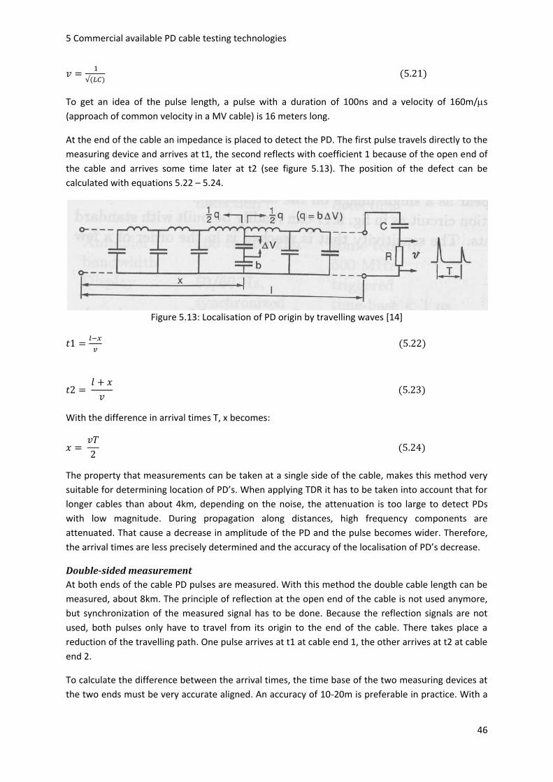
5 Commercial available PD cable testing technologies
46
To get an idea of the pulse length, a pulse with a duration of 100ns and a velocity of 160m/s
(approach of common velocity in a MV cable) is 16 meters long.
At the end of the cable an impedance is placed to detect the PD. The first pulse travels directly to the
measuring device and arrives at t1, the second reflects with coefficient 1 because of the open end of
the cable and arrives some time later at t2 (see figure 5.13). The position of the defect can be
calculated with equations 5.22 – 5.24.
Figure 5.13: Localisation of PD origin by travelling waves [14]
With the difference in arrival times T, x becomes:
The property that measurements can be taken at a single side of the cable, makes this method very
suitable for determining location of PD’s. When applying TDR it has to be taken into account that for
longer cables than about 4km, depending on the noise, the attenuation is too large to detect PDs
with low magnitude. During propagation along distances, high frequency components are
attenuated. That cause a decrease in amplitude of the PD and the pulse becomes wider. Therefore,
the arrival times are less precisely determined and the accuracy of the localisation of PD’s decrease.
Double-sided measurement
At both ends of the cable PD pulses are measured. With this method the double cable length can be
measured, about 8km. The principle of reflection at the open end of the cable is not used anymore,
but synchronization of the measured signal has to be done. Because the reflection signals are not
used, both pulses only have to travel from its origin to the end of the cable. There takes place a
reduction of the travelling path. One pulse arrives at t1 at cable end 1, the other arrives at t2 at cable
end 2.
To calculate the difference between the arrival times, the time base of the two measuring devices at
the two ends must be very accurate aligned. An accuracy of 10-20m is preferable in practice. With a

5 Commercial available PD cable testing technologies
47
common speed of about 160m/s in cable, the time difference to reach an accuracy of 16m is 100ns.
The alignment of the time base can be done in different ways:
GPS
Pulse injection
GPS
Satellites of the GPS system send information about place and time to earth. The time between the
arrival times of information coming from different satellites, can be used for determining the
position of the receiver on earth. It takes at least four satellites to determine the three location
coordinates and the time, but more satellites increase the accuracy. A disadvantage is that the
satellites have to be visible for the receiver, large buildings can distort the signal. Also there can be
some small errors in the determination of the arrival times of the signals from different satellites.
This lead to an error in the time and location. Furthermore the signal of the satellite travel through
variations in atmosphere that also brings errors in arrival time.
Nevertheless in practice the accuracy is still high and is behind the limit of 100ns. To gain more
accuracy, DGPS can be used. This makes use of a reference receiver at a known place. Because the
known position of the reference receiver, the time errors can be calculated. DGPS has an accuracy of
5-20ns (about 1-5m)
Pulse injection principle
For pulse injection pulse sensor / injections units (SIU) are needed. When a pulse is injected at one
side of the cable, it can be measured at the other side of the cable. When the other SIU receives the
pulse, it immediately sends a pulse back. [25]. The travelling time of the pulse through the cable can
be gained out of the arrival time of the pulse at end 1 and injection time. When the travel time of the
pulse is known, the time bases of the two units can be aligned. The cable is used for transmission of
the information, in this way the system is not influenced by factors from outside. Furthermore the
accuracy is even higher than GPS and the used equipment is less expensive.
5.4 On-line measurements
5.4.1 Introduction
Online PD measurement is a very useful tool for condition based maintenance. The first advantage is,
that in theory, the cable doesn’t have to go offline. The cable is measured during operation, so loads
can stay connected and the energy transport through the cable can continue during measurements.
This has a great advantage in case redundancy is not available. In practice it is not allowed to place a
sensor at some position around a conductor or earth wire when the cable is still in service, but
installing the sensor takes a very short time.
Because the cable is measured online, the measurement is sort of continuous. In comparison with
offline measurement there is made a ‘movie’ instead of a snapshot of the PD activity. Because online
PD measurement systems can measure full time for days [31], developing of the PD activity in time
can be measured, and trend watching is possible. In this way condition based maintenance can be
applied more accurate.

5 Commercial available PD cable testing technologies
48
During online PD measurement only PD is measured initiated by the operating voltage. This brings
the same stress as during operation. This has advantages and disadvantages. When the cable is taken
offline for installation of the sensor, PDs that have initiation voltage above operating voltage will not
initiate before a transient overvoltage has reached the cable. On the other side, PDs with initiation
voltage and extinction voltage both above the operating voltage are not triggered and these defects
will not develop.
Because online PD measurement doesn’t require an external source, equipment is small and
handsome.
5.4.2 Principle
Online PD measurement systems can measure at one single point or at both ends of a cable.
Single point measurement
Measurement systems that measure at a single point makes use of TDR to locate the origin of the PD
in the cable. This method of localization is described in chapter 5.3. For long cables, or cables with
high PD signal attenuation, there could be used a transponder. This transponder is placed at the
remote end of the cable. When the pulse half of the that is travelling to the remote end arrives at the
transponder, the transponder injects a large pulse that is travelling to the beginning of the cable. In
this way, the time difference between the otherwise small reflected pulse is measured properly.
Double side measurement
In case there is measured at two sides of the cable, the system makes use of two measurement units,
each at an end of the cable. Thereby the time bases are aligned by GPS time signal or by the pulse
injection method (see chapter 5.3). Figure 5.14 shows a simplified scheme of system that measures
at two sides of the cable. Because online measurement systems can be placed in a substation or in a
ring main unit (RMU), they are exposed to lots of noise and interference signals, often with
amplitudes larger than the PD signals. Therefore the triggering of the measuring hardware cannot be
implemented simply. During monitoring not every PD has to be measured. The target is to give a
representative view of the cable condition. When real time monitoring is applied, huge data
processing capacity is needed. To give a representative view of the PD’s in the cable and to reduce
the amount of data, only cycles of 30ms are measured. The measuring units get a trigger signal from
GPS or a synchronisation pulse from the cable that is higher than the rest of the signals. The time of
recording data depends on the power frequency of the cable. The 50Hz grid has a period of 20ms;
therefore time to record data is 30ms including the trigger pulse and the analysed data block.
Figure 5.14: Simplified scheme of an online PD measurement system [26]

5 Commercial available PD cable testing technologies
49
PDs are filtered out of the data blocks, to reduce the data stream to the interpretation unit. A
communication via TCP/IP link is set up between the data acquisition devices and an interpretation
unit. The results are combined, interpreted and it is done some PD analysis. Invalid PD’s are rejected
and the valid PD’s are kept. The results are stored and displayed at a computer with a user interface.
5.4.3 Equipment
Hardware
The equipment of a single point measurement system can be simpler than equipment of a multiple
point measurement system. This is because there doesn’t have to be synchronization between two
measurement units. Equipment could consist of a high current transformer, and an advanced
oscilloscope with a large bandwidth of some hundreds of MHz and specially made PD measurement
software.
Figure 5.15 shows a scheme of hardware components of a measurement device that measures at
two sides of the cable. The sensors are high frequency current transformers, clamped around earth
wire or insulated cable in a RMU or substation. From the sensor, the measured values are amplified
and go to a data acquisition card in the computer. The PC in the control unit does some analysis of
the data. Further the system has a GPS receiver for synchronization of time bases and a pulse
generator to align time bases.
Figure 5.15: Hardware of one measurement setup [26]
Sensors and filters
For PD measurement at two sides of the cable, there are required two devices to measure PDs, one
at each side of the cable. Each of these two measurement units makes use of a sensor/injection unit
(SIU). The unit can measure PD pulses as well as inject a pulse into the cable. The sensors are high
frequency current transformers and injection coils, that can be clamped easily around the earth wire
of around the insulated conductor. In this way the system can stay online while assembling the
setup. Next to this practical advantage, safety has also to be considered. There is no galvanic
connection between sensor and conductor; therefore it is very difficult for high voltage to reach the
control equipment.
Used split core current transformers have bandwidths that start around 100kHz and end at tens of
MHz. The filter in the control unit strongly filters the 50Hz power frequency out of the signal.

5 Commercial available PD cable testing technologies
50
For PD measurement at a single location, HFCTs can also be used. Commercial systems also use
HFCTs with bandwidths starting at about 100kHz until about 25MHz. Next to these filters, there can
be added extra filters in noisy environments. There are high pass filters with a low cutoff frequency
of 100kHz and low pass filters with a cutoff frequency of 70MHz. There can also be applied filters in
the software.
PD analysis
When the waveform of the PDs is known, matched filtering can be applied. It causes a maximum
SNR. To determine the desired transfer function of the filter, the frequency spectrum of the PD signal
and the frequency spectrum of the noise have to be determined. The signal first meets a whitening
filter that determines the noise spectrum out of present and previous data. Also a notch filter is
applied to filter narrow band radio broadcast signals. For the determination of the PD spectrum, the
transfer function of the sensor is needed and the load impedance of the RMU. After spectrum
determination, a matched filter bank can be applied. Any other filter than the matched filter gives a
lower output signal.
To analyse the data of the records, the time bases have to be aligned to compare the data with each
other. As already mentioned synchronization of the time bases of the two measurement devices can
be done by GPS, or by pulse injection. The pulse generator and injection coil inject pulses with very a
very high accuracy to 30ms in between. If we combine the pulse propagation time with the arrival
times of the accurate synchronization pulses, the time bases of the two can be aligned. Of the
interval between two reference pulses, a 50Hz period is used for PD extraction. A central computer
downloads the data from the measuring units and combines this data by finding pairs of pulses that
satisfy the condition:
In this way signals from outside are skipped.
Also the polarity of the measured pulse can be used to determine whether the pulse is from inside or
outside the cable.
For single point measurement, distinction between measured polarity cannot be used to determine
where the pulse in coming from.
The polarity of the PD pulse can cause a positive or negative measured pulse at the HFCT. Next to
that, also the direction the pulse in coming from can cause a different measured polarity. Because
only current is measured, determination of the direction of the energy flow by use of the poynting
vector cannot be used. Pulses that have their origin inside a substation, have commonly other shapes
than a pulse that has travelled through a cable. This property is used to determine whether the pulse
is coming from the cable or not.
Practical usage of the online measuring system
Online PD measurement devices just have the size of a modern oscilloscope and weights less than
10kg, so it is very easy to handle. It requires a supply voltage of 90-264V AC. Online PD measurement
is used successfully from 3.3kV up to 750kV [31]. To assemble a measuring setup, it takes about 5-10
minutes.

5 Commercial available PD cable testing technologies
51
5.5 Summary and conclusions Now we have considered online and offline measurement methods. Their principles, equipment and
their practical usage. An overview of the most important parameters of the energizing sources are
shown in table 5. Every system has its advantages and/or disadvantage at different subjects.
For measuring, capacitive and inductive sensors are used. Capacitive sensors have a higher
sensitivity, but inductive sensors are galvanic separated of the test object. Furthermore inductive
sensors with a low lower cutoff frequency have a lower gain within their bandwidths than HFCTs with
a higher low cutoff frequency.
For localization of the defect in a cable, TDR can be used. Also measurement at double side of the
cable can be applied. This doubles the maximum length that can be measured, but the method
requires synchronization of the measured signals.
When comparing online with offline measurement, a significant difference is the possibility of trend
watching of PD activity. With online measurement it is not possible to detect all the defects in the
test object. Therefore use of online and offline methods could be useful when it is desired to create a
complete picture of the defects in the cable.

5Commercial available PD cable testing technologies
52
Table 5.5: Global comparison of PD measurement voltage sources
Properties of Cable energizing methods
Stress compared with service stress
Most important difference with 50Hz/60Hz
Voltage range used
Load capacitance
Duty IEC60270 compatible
Weight and volume
transportability
Suitability field measurement
50/60Hz AC Identical No difference MV and HV small compared with other sources
continuous Yes Large and heavy comparing with the other methods
No transport possible
Not suitable
VLF Different Very low frequency, higher inception voltage. Deposited charge at cavity walls has more time to leak away
28kV – 200kV peak
Several km continuous Yes Small Even HV units can be transported in a van
Very handy
Damped AC with OWTS
Very similar Damped voltage. Energizing shots, large amount of shots needed. Because short duration of shots, virgin cavities are probably not detected, but also not activated
28kV – 250kV peak
Several km In shots with damping of the signal
Yes, in case frequency < 400Hz
Small Even HV units can be transported in a van
Very handy
Resonant system Close to 50Hz When frequency is kept below 200Hz, there is no big difference
55kV – 400kV Several km continuous Yes Large and heavy comparing with the other methods
For MV a heavy van is needed to transport, for HV a truck
More difficult to transport and to position next to object, so less suitable
Online Identical Only transient overvoltages can initiate PD with Vi above operating voltage. PD with Vi and Ve above operating voltage are probably not initiated
3.3kV -750kV cables
As long as the cable is
continuous Yes Small Non applicable
Very easy to install

6 Partial discharge measurements, conventional and unconventional
53
6.1 Introduction When comparing different PD measurement methods, it can be remarked that there are systems
that measure according to the IEC60270 (conventional way of measuring), but that there are also
systems that do not measure according to the standard. In this chapter we explain conventional and
unconventional measurements and we investigate why measuring according to the IEC standard is
not always suitable for PD measurement in cables. An explanation is given why unconventional
measurement is needed. We can make a distinction between two types of PD measurements.
Conventional (this is according to the standard for partial discharges IEC60270)
Unconventional (not following the IEC60270 standard)
6.2 Conventional measurement
6.2.1 Introduction
This chapter describes how conventional PD measurement works. Next to this, it gives insight into
conditions for measuring according to the standard, compares different settings within the
prescribed margins of the standard and shows the limits of this method for measurement of PD in
MV cables.
6.2.2 Standard
The IEC 60270 standard is an international standard for measuring Partial Discharges. PD’s that occur
in electrical components, devices or systems when tested with alternating voltages up to 400 Hz or
with direct voltage.
This standard
defines the terms used;
defines the quantities to be measured;
describes test and measuring circuits which may be used;
defines analogue and digital measuring methods required for common applications;
specifies methods for calibration and requirements of instruments used for calibration;
gives guidance on test procedures;
gives some assistance concerning the discrimination of partial discharges from external interference.
The terminology, definitions, basic test circuits and procedures often also apply to tests with other frequencies, but special test procedures and measuring system characteristics, which are not considered in this standard, may also be required.[9]
6 Partial discharge measurements, conventional and
unconventional

6 Partial discharge measurements, conventional and unconventional
54
PD pulse Measured
with sensor
IEC Bandpass
filter
Peak value charge
* kcal charge
6.2.3 Description conventional PD measurement
The procedure of conventional PD measurement is shown in figure 6.1. A typical measurement setup
is shown in figure 5.11. From right to left there is shown the high voltage supply with blocking
inductance (filter) to block discharges of the supply into the measurement system. The High voltage
source with filter supplies voltage to the test object, depicted as a capacitor (for example a cable).
Parallel to this, in series, is placed a filter consisting of a coupling capacitor and a measuring
impedance. This filter takes care for filtering the power frequency and its harmonics. The sensor, or
measuring impedance, measures the input PD current pulse and transforms it into an output voltage.
After measuring the PD pulse, the signal is filtered with specifications according to the IEC60270
standard. Figure 6.2 shows that a very small piece of the total frequency spectrum of a PD pulse
passes the IEC filter. Therefore, the time response output signal of the filter has a totally different
shape than the original PD pulse.
The charge is determined by the fact that the peak value of the output signal is proportional to the charge. By means of a calibrator that injects a known charge, the system can be calibrated. After calibration, the system can be used for charge determination of PD pulses with different magnitudes.
Figure 6.1: Process of conventional PD measurement
Figure 6.2: Frequency spectrum of a calibrator pulse and the IEC bandwidth 30kHz-400kHz
0 2 4 6 8 10 12 14 16 18 200
500
1000Frequency spectrum PD pulse
MHz
mV
Frequency spectrum PD pulse
IEC filter bandwidth
0 0.2 0.4 0.6 0.8 1 1.2 1.4 1.6 1.8 2600
700
800
900Frequency spectrum PD pulse zoomed in
MHz
mV
Frequency spectrum PD pulse
IEC filter bandwidth

6 Partial discharge measurements, conventional and unconventional
55
6.2.4 Prescriptions of the IEC60270 standard for measuring PD
This chapter handles the most important things that have to be fulfilled to measure PD according to
the standard.
Coupling device
The measuring impedance, also known as coupling device, often forms one unit with a high voltage
coupling capacitor (see figure 6.3). When a PD pulse arrives at the measurement location, it sees a
different impedance. The combination of coupling capacitor has to fulfil:
High impedance for the operating frequency.
Only the low voltage PD signal should be measured with the measuring impedance
The combination of coupling capacitor and measuring impedance acts as a filter with as output the
measuring impedance. The low cutoff frequency of this filter has to be tuned in a way that at least
the power frequency signal and its harmonics are filtered out. Next to this, the measuring impedance
only measures the high frequent signals.
Figure 6.3 is shows an example of a measuring coupling capacitance and measuring impedance.
Together they must have a very large impedance at 50Hz to avoid large currents to be flown.
When assuming all operating voltage stands over the coupling capacitor, the current that is flowing
through the combination of measuring impedance and coupling capacitor becomes:
Where
Umax = the maximum test voltage
f = frequency of the test voltage
C = coupling capacitance
When having a large characteristic impedance in comparison with the measured MV cable, the
voltage reflection coefficient is approximated by 1. In that case there is a doubling of the voltage of
pulses achieved at the measuring point. This is preferable to gain high sensitivity.
Coupling capacitor
Measuring impedanceMeasuring device
Figure 6.3: RLC measuring impedance with coupling capacitor
The standard prescribes that the coupling device should filter at least the test voltage and its
harmonics for reaching the measuring equipment.

6 Partial discharge measurements, conventional and unconventional
56
Measuring instrument
After measuring PD with a combination of coupling capacitor and measuring impedance, the signal
arrives at the measuring instrument, see figure 5.11. At this point a filter, specified according to the
standard, filters the signal. To achieve good results, it is important that the bandwidth of the
measuring impedance in combination with the coupling capacitor lies within the IEC specified
bandwidth. To avoid errors, a pulse train response show give a flat amplitude of frequency response
within the bandwidth of the IEC filter. This bandwidth is shown in figure 6.4.
Figure 6.4: Correct bandwidth example for measuring PD in conventional way
When measuring PDs according the standard, there are two kinds of bandwidths specified for the IEC
filter. There can be measured with narrow band and with wide band. The bandwidths are specified as
follows:
Wide band
o
o
o
It is important that the bandwidth of the sensor is overlapping completely the bandwidth of the IEC
filter, to get correct measurement values for the charge of PDs. In case no filter is used, the
bandwidth of the sensor must fulfil the IEC bandwidth. The standard prescribes an adequate
attenuation below f1 and above f2, so there is a range left to implement this adequate attenuation.
The effect of the order of filter, will be investigated later on.
The second type IEC filter is called narrow band filter. It uses a very narrow bandwidth compared to
wide band. The specifications are described as:
Narrow band
o
o
Where stand for the width of the band and fm is the centre frequency. It can be shown that the
bandwidth can vary between 9 and 30 kHz. With the chosen bandwidth, the band can be shifted in
the frequency spectrum where the amplitude of the frequency spectrum of the PD pulse is more or
less constant (about between 50kHz and 1MHz, which depends on the pulse). Onwards it is not

6 Partial discharge measurements, conventional and unconventional
57
recommended to use a sensor with a bandwidth that does not completely overlap the band of the
filter.
Furthermore it is recommended that the transfer impedance at frequencies of fm should be
20dB below the peak pass-band value. [9].
A difference between the wide band and the narrow band method is the pulse resolution time. The
pulse resolution time is the shortest time between two consecutive short pulses with the same
shape, charge and polarity for which the peak value of the resulting response will not change more
than 10% of that for a single pulse. In general the pulse resolution time is inversely proportional to
[9]. This means the wider the bandwidth of the system, the smaller the pulse resolution time.
When the arrival time between PD’s is shorter than the pulse resolution time, there has been made
an error in the measurements. The pulse resolution times for the different bandwidths are:
Wide band pulse resolution time
o 5s - 20
o In practice < 10s
Narrow band pulse resolution time
o > 80s
[9]
6.2.5 Limits of the conventional measuring method
In this chapter it is explained how to calibrate an IEC system and why, the influence of the order of
the filter is determined and the limit of pulse width is treated.
Charge determination
When calibrating the IEC system for a certain value and pulse shape, all the measured pulse response
peaks that the system is going to measure must be proportional to the calibrated value. A calibrated
system with a pulse of 500pC must measure a PD with a charge of for example 100pC also correctly
by measuring its proportionality to the calibration peak pulse response.
Because of the proportionality property of the system, pulses with different charge but with the
same shape show linear related peak values in the time response. In case calibrating and checking if
the system is proportional to different pulse shapes, using the same pulse shape but different charge,
does not make sense.
Desired is to measure different kinds of pulse shapes with only a single calibration. Therefore the
frequency spectrum of the calibrator pulse has to be approximately constant within the bandwidth of
the IEC filter. To achieve this, the standard prescribes that the IEC system has to be calibrated by a
calibrator pulse that has a rise time< 60ns. By pulses with longer rise time, decay of the frequency
spectrum takes place at lower frequencies. This can be obtained of figure 6.5
In figure 6.5 the frequency spectrum of 4 real pulses, measured with a sensor that has a low cutoff
frequency of 10kHz, are plotted. This is chosen because a combination of coupling capacitor and
measuring impedance can reach such value of low cutoff frequency. Also the frequency responses of

6 Partial discharge measurements, conventional and unconventional
58
the filtered signals by different orders are plotted. The IEC bandwidth 30kHz – 400kHz is used. Table
6.1 shows the properties of the used pulses.
Table 6.1: Most important properties of the pulses used for described experiments
Used calibrator q inj. q at measuring point
Travelled distance through MV cable
Rise time
Decay time
3706 500pC 421,5pC 640m (first reflection) 41,2ns 108,8ns
3706 500pC 398,8pC 1920m (second reflection) 91,6ns 410,4ns
3706 500pC 340,5pC 3200m (third reflection) 140,4ns 699,2ns
3706 500pC 300,1pC 4480m (fourth reflection) 186ns 1165,6ns
Figure 6.5: Frequency spectra of the measured calibrator pulse signals and of the IEC filtered signals
As displayed in figure 6.5 only the first reflection has a flat frequency response in the region of the
IEC wide band bandwidth. Only this pulse can be used to calibrate the system. It can also be observed
in table 6.1 that reflections 2,3 and 4 have a longer rise time than 60ns and therefore are not
recommended for calibration. In figure 6.6 the peak of the IEC filter output against the real charge of
the reflections 1,2,3 and 4 that is measured with UWB is plotted. The pulses and filter of figure 6.5
are used to plot these reflections. Next to the frequency responses, the proportionality line from the
calibration pulse charge to the origin is plotted.
0 0.1 0.2 0.3 0.4 0.5 0.6 0.7 0.8 0.9 10
5
10
15
20
25
30
35
X: 0.9875
Y: 26.22
MHz
mV
Frequency spectra reflections calibrator pulse and IEC response spectra
first reflection
second reflection
third reflection
fourth reflection
order2 filter
order4 filter
order6 filter
order8 filter

6 Partial discharge measurements, conventional and unconventional
59
It shows that a large error has been made in approaching the proportionality line by the measured
peak values for the charges of the different pulse shapes. This is caused by the non flatness in the
frequency spectrum of reflections 2, 3 and 4 of the pulses.
Figure 6.6: Peak value IEC filter vs. real charge of input pulse
Figure 6.7: Peak value IEC filter vs. real charge of input pulse
To reduce the error in charge determination, the bandwidth can be narrow, while the low cutoff
frequency is kept at the lowest value possible. In figure 6.7 a bandwidth of 30kHz-200kHz is used. It
shows that the error has become smaller. This is due to the less differentiation in frequency spectra
between the first reflection and the other three. A drawback is that the error made by measuring
320 340 360 380 400 4200.4
0.5
0.6
0.7
0.8
0.9
1IEC peak value vs real charge with 30kHz-400kHz IEC filter
real charge
IEC
peak v
alu
e [
P.U
.]
order2 filter
order4 filter
order6 filter
order8 filter
calibration line to origin
320 340 360 380 400 4200.55
0.6
0.65
0.7
0.75
0.8
0.85
0.9
0.95
1IEC peak value vs real charge with 30kHz-200kHz IEC filter
real charge
IEC
peak v
alu
e [
P.U
.]
order2 filter
order4 filter
order6 filter
order8 filter
calibration line to origin

6 Partial discharge measurements, conventional and unconventional
60
pulses in the non flat region is related to the steepness of the decay of the frequency spectrum of a
pulse.
In case there has to be dealt with wide pulses, the bandwidth of the IEC filter can be narrowed while
keeping the low cutoff frequency the same. In this way, the filter bandwidth is moved to the area
where the spectra are more flat. The second, third and fourth reflections of the sequence of pulses
start with the decay of its high frequency content at about 80kHz. Because wide band prescribes a
low cutoff frequency of 30kHz and a minimum bandwidth of 100kHz, puts the high cutoff frequency
at 130kHz. The decay of the frequency spectra of the reflections 2, 3 and 4 lie within this bandwidth.
Therefore measuring these pulses with wide band IEC filtering is less accurate.
The narrow band filter is suitable for measuring this width of pulses. Narrow band is also applied,
using a bandwidth of 50kHz-80kHz. In this case the approach of the peak values to the
proportionality line of calibration is relatively good, as figure 6.8 shows. This figure plots the
relationship between IEC filter peak value and the real charge normalized to the peak value of the
first reflection. With the order 8 filter the highest accuracy achieved.
When comparing the time responses of wide band 30kHz-400kHz and narrow band 50kHz-80kHz, the
time response of the narrow band is, as mentioned before, indeed far longer. These time responses
are expressed in figure 6.9. Another thing that can be remarked is that the polarity of the wide band
time response is clearly recognizable by the first peak, but that is not the case with narrow band
because the signal is very more oscillating. Therefore it is not possible to determine the polarity of
the PD pulse with narrow band.
Figure 6.8: Peak value IEC filter vs. real charge of input pulse
320 340 360 380 400 4200.65
0.7
0.75
0.8
0.85
0.9
0.95
1IEC peak value vs real charge with 50kHz-80kHz IEC filter
real charge
IEC
peak v
alu
e [
P.U
.]
order2 filter
order4 filter
order6 filter
order8 filter
calibration line to origin

6 Partial discharge measurements, conventional and unconventional
61
Figure 6.9: Time responses of calibrator pulse, wide band and narrow band filtered
Superimpositioning of consecutive pulses
This chapter will show the error that can be made in case two consecutive pulses separated by time
that is less than the pulse resolution time.
As already mentioned, the response of an IEC filter to a very short pulse in a MV cable takes far more
time than the original signal. We are going to determine the pulse resolution time of a MV cable.
There is a 1nC calibration pulse injected into the MV cable and recorded with an oscilloscope using a
bandwidth from DC to 300MHz (Ultra Wide Band, UWB). The data is imported in Matlab and
afterwards filtered. A signal of two consecutive pulses has been made. The distance between the
pulses can be varied by adding a demanded number of zeroes between the pulses. The signal is put
into an IEC filter and the time response is given in figure 6.10.
As already mentioned, to reach the pulse resolution time according to IEC60270, it is required that
the response of the filter to two consecutive pulses does not differ more than 10% of the response
value to one single pulse.
To create the shortest pulse resolution time, we take the 30kHz-430kHz bandwidth to filter the input
signal of the two consecutive pulses. In figure 6.10 the response of the filter to the pulse in a MV
cable is displayed. The superposition error is clearly visible.
0 50 100 150
-1.5
-1
-0.5
0
0.5
1
s
Outp
ut
IEC
filt
er
[V]
IEC filter time response wide band and narrow band
narrow band 50kHz-80kHz
wide band 30kHz-400kHz

6 Partial discharge measurements, conventional and unconventional
62
Figure 6.10: Two consecutive input pulses and their IEC filter output response
A summation of the advantages and disadvantages of conventional measuring method is made in
table 6.2.
Table 6.2: Advantages and disadvantages of IEC wide band and narrow band PD measurement
Wide band Narrow band
Advantageous Compared with narrow band a relative short pulse resolution time
(In general the pulse resolution time is inversely proportional to BW)
Polarity can be easily gained out of the response signal
Sensors with a relative high low cutoff frequency can be used
Disadvantageous Sensor with a relative low cutoff frequency needed
Cannot measure correctly pulses as long as the narrow band can measure.
A long pulse resolution time
Polarity cannot be gained out of the output signal
0 1 2 3 4 5 6 7 8-0.05
0
0.05
0.1
0.15V
[s]
Consecutive pulses
Input signal, two identical consecutive pulses
0 5 10 15 20 25 30 35 40 45 50-10
-5
0
5
10System response with 30kHz-400kHz IEC filter
[s]
mV
Response of system on two identical consecutive pulses
response on one single pulse

6 Partial discharge measurements, conventional and unconventional
63
6.2.6 Feasibility conventional measurement method for PD measurement in MV cables
This subchapter handles the feasibility of the IEC method for PD measurement in MV cables. Thereby
the two topics discussed are:
Charge determination
Localization
First the suitability of conventional measurements method for measuring the charge of PD in MV
cables is investigated, afterwards the suitability for localization has been researched.
During PD pulse propagation in the cable, the damping of the high frequency content of PD pulses is
large. Therefore the flat region in the measured frequency spectrum begins at the lower cutoff
frequency of the sensor and ends at a more and more lower frequency.
Therefore, the wide band measurement method becomes less suitable for measuring pulses that
have to travel a distance through the cable that is too long. As shown in figures 6.6 and 6.7,
measuring pulses with travel paths between 0 and 1.3 km give already an error. With narrow band,
the charge of a sequence with short and wide pulses can be determined with a good accuracy, but
the pulse resolution time is very large.
The pulse resolution time of the wide band method is approximately between 5s and 20s,
depending on the bandwidth of the filter. So to have no integration error caused by super positioning
of the response of two consecutive pulses, there has to be 5s -20s between arrival times of the
pulses at the measuring location.
(6.1)
Figure 6.11: Model of a cable with a defect that produces PD
In case there is PD in cables, measured with the conventional method, superimposition of responses
have to be taken into account, as mentioned before. The time between pulses has to be equal or
larger than the pulse resolution time. Half of the PD pulse is travelling from the defect to the
beginning of the cable and the other half to the end. It reflects there and travel to the beginning of
the cable. Therefore it can occur that the differences in arrival times of the two half pulses are equal
of more than the pulse resolution time. This is the case when a defect in a cable is x meters away
from the cable end, as shown in figure 6.11. There is PD measured with an error in case the defect is
in cable length x, because of superimposition of pulse responses. The distance one half of the PD
pulse has to travel with velocity v through the cable to gain an extra travelling time that fulfils the
pulse resolution time is equal to 2*X.

6 Partial discharge measurements, conventional and unconventional
64
When we use some practical values to get an idea of length of x we take:
(6.2)
(6.3)
Therefore
(6.4)
(5) (6.5)
This is a long distance in comparison to the total cable lengths of 1-4km that are measured. Next to
this, it cannot be recognized if superimposition of pulses is measured.
This in combination with determination of charge of wide PD pulses that travelled distances longer
than 2km through a MV cable, gives the conclusion that conventional PD measurement could give an
error in charge determination of PD in MV cables.
Because of superimposition of pulse responses, arrival times of pulses could not be determined.
Therefore conventional measurement is not suitable for defect localization with TDR in power cables.
6.2.7 Conclusion
At the moment conventional measurement is the only measurement method that is described in a
standard. The standard describes the conditions for this measurement and the calibration method.
For calibration, only steep pulses can be used, with rise time < 60ns. It is also recommended that the
frequency responses of the PD pulses that are predicted to measure are flat within the bandwidth of
the IEC filter. Therefore with wide band can be measured accurate relatively small pulses, with travel
distances in a MV cable of about 1km. With narrow band wider pulses until couple of km’s can be
measured with high accuracy. Because the time response is proportional to the inverse of the
bandwidth, the smaller the IEC bandwidth, the longer pulse resolution time. Because of the long time
response, the widest bandwidth has to be used, but therefore only steep pulses can be measured,
hence pulses with short travelling distances. Because of the long time response, an error can be
made in determination of charge, when PDs are measured of a defect that is within distance x from
the end of the cable. The combination of the length of the time response and the width of the PD
pulses that can be measured with high accuracy makes conventional measurement less suitable for
measuring PD in cables.
6.3 Unconventional measurements
6.3.1 Introduction
As discussed in the previous chapter, for PD measurement in cables it is desirable to measure a short
pulse response. This will reduce errors in charge determination and makes defect localization
possible. Because of the long response time of the conventional method, unconventional
measurements are needed. Due to the fact that there is no standard for unconventional

6 Partial discharge measurements, conventional and unconventional
65
measurements, different systems are used with different sensors that measure different pulse
responses.
To be sure the cable meets its prescribed quality, it is measured for PD at the factory. After shipping
and placing, but before taking the cable into service, a commissioning PD test is taken. Often
different kind of PD measurement systems are used. To be sure the placed cable still fulfils the
prescribed quality which it had at the factory, the measurements of the sometimes different systems
have to be comparable. Often, this is not the case.
In this chapter we investigate different kinds of methods that could make possible comparison
between conventional and unconventional measurements and between unconventional
measurements using different sensors.
First we investigate the influence of different sensors on the response of a PD pulse, secondly we
compare different methods for determination of charge, measuring with different sensors simulated
by digital filters. Afterwards PD pulses are measured with real sensors and the results are compared.
6.3.2 Influence of the sensor on the PD pulse response.
Because there is no standard for unconventional PD measurement, different PD measuring systems
use different sensors that give different pulse responses. In this chapter we are investigating the
influence of different sensors on the PD pulse response. The different sensors are simulated by a
second order filter with different bandwidths.
To investigate the influence of the BW of the sensor on the pulse response there is used an UWB
recorded pulse of 859pC, generated by injecting a 1000pC with the 3706 Haefely calibrator that has
to travel 640m through a MV in order to reach the measurement point. First the pulse is filtered only
with a high pass filter with different low cutoff frequencies. For low cutoff frequencies are used 0HZ
(UWB), 10kHz, 50kHz, 100kHz, 200kHz, 500kHz and 1000kHz. Figure 6.12 shows the time response,
their integral and the frequency spectra of the UWB signal and the filtered signals.
It shows that the higher the low cutoff frequency, the higher is the negative overshoot of the
response and the shorter the length of the pulse. The short time response is useful to decrease the
pulse resolution time. The integral of the pulse goes to zero. The higher the low cutoff frequency, the
faster it reaches the value of zero. This is caused by the fact that the integral of the response of a
high pass filter always goes to zero because the DC component is filtered out of the signal.
When we look at the time response, we see that the lower the low cutoff frequency, the more the
highest peak looks like the original signal. Integration of this highest peak could approach the charge.
The peak of the integral corresponds to the zero crossing of the signals. Figures 6.20-6.24 show that
this is an accurate method for determination of charge for the first two reflections, if a sensor is used
with a low cutoff frequency below 10kHz.
Now we are going to take the same test, but for the pulses measured after travelling 3200m. Figure
6.13 shows the results. We see that the high frequencies are strongly attenuated. We also see that
the length of the time responses of the filtered signals are about the same as from the pulse that has
travelled 640m, while the length of the original UWB pulses is much longer than the UWB pulse of
figure 6.12. When comparing the shapes of the filtered signals and the UWB signal, there is more
difference between them by the pulse that has travelled 3200m than 640m. Determination of charge

6 Partial discharge measurements, conventional and unconventional
66
by integrating the first peak becomes worse. Figure 6.14 shows the first peaks of the two pulses.
When comparing the amplitudes of the two UWB signals, it is expressed that the 3200m signal has
very less amplitude than the 640m signal. This is causes by attenuation of the high frequencies during
propagation of the pulse through the cable. When comparing the peaks of the time responses of the
different filters (see figure 6.14), we see that sensitivity of the 3200m pulse decreases stronger than
from the 640m pulse. The high frequency content of the 3200m pulse reaches until about 200kHz. It
explains that measuring with a low cutoff frequency above 200kHz decreases the sensitivity strongly.
It shows for these pulses, that measurement of pulses that have travelled through the cable for a
long distance, measured with a system with a relative high lower cutoff compared with the
frequency content has a relative low sensitivity.
Now the high cutoff frequency is investigated and a low pass filter is used to do so. For the high
cutoff frequencies is taken: 10MHz, 2MHz, 1MHz, 800kHz, 400kHz. Figure 6.15 shows the results.
When the high frequencies are filtered, the sensitivity decreases strongly. Furthermore the pulse
becomes wider, this is the same that happens during propagation through the cable. Next to this, the
rise time decreases, by a lack of dispersion (see chapter 4). The integral of the signal is not influenced
by filtering high frequencies, which 6.15 also shows. This is logical because the DC component is not
filtered out.

6Partial discharge measurements, conventional and unconventional
67
Figure 6.12: Time responses, integrals, frequency spectra of UWB signal and filtered UWB signal with different low cutoff frequencies for pulse that has
travelled 640m through a MV cable
0 500 1000 1500 2000-0.06
-0.04
-0.02
0
0.02
0.04
0.06
0.08
0.1
0.12
0.14
ns
V
Time responses
UWB signal
10kHz low cutoff
50kHz low cutoff
100kHz low cutoff
200kHz low cutoff
500kHz low cutoff
1000kHz low cutoff
0 2000 4000 6000 8000 10000-10
-5
0
5
10
15
20
25
30
35
ns
mV
Integral
UWB signal
10kHz low cutoff
50kHz low cutoff
100kHz low cutoff
200kHz low cutoff
500kHz low cutoff
1000kHz low cutoff
0 0.2 0.4 0.6 0.8 10
5
10
15
20
25
30
35
MHz
mV
Frequency spectra
UWB signal
10kHz low cutoff
50kHz low cutoff
100kHz low cutoff
200kHz low cutoff
500kHz low cutoff
1000kHz low cutoff

6 Partial discharge measurements, conventional and unconventional
68
Figure 6.13: Time responses, integrals, frequency spectra of UWB signal and filtered UWB signal with different low cutoff frequencies for pulse that has
travelled 3200m through a MV cable
0 2000 4000 6000 8000 10000-0.01
-0.005
0
0.005
0.01
0.015
0.02
ns
V
Time responses
UWB signal
10kHz low cutoff
50kHz low cutoff
100kHz low cutoff
200kHz low cutoff
500kHz low cutoff
1000kHz low cutoff
0 2000 4000 6000 8000 10000-5
0
5
10
15
20
25
ns
mV
Integral
UWB signal
10kHz low cutoff
50kHz low cutoff
100kHz low cutoff
200kHz low cutoff
500kHz low cutoff
1000kHz low cutoff
0 0.2 0.4 0.6 0.8 10
5
10
15
20
25
MHz
mV
Frequency spectra
UWB signal
10kHz low cutoff
50kHz low cutoff
100kHz low cutoff
200kHz low cutoff
500kHz low cutoff
1000kHz low cutoff

6 Partial discharge measurements, conventional and unconventional
69
Figure 6.14: Zoom in first peak time response of figures 12 and 13 respectively
200 250 300 350 400 450
-0.04
-0.02
0
0.02
0.04
0.06
0.08
0.1
0.12
ns
V
Time responses 640m travelled
UWB signal
10kHz low cutoff
50kHz low cutoff
100kHz low cutoff
200kHz low cutoff
500kHz low cutoff
1000kHz low cutoff
0 100 200 300 400 500 600 700 800 900 1000-0.01
-0.005
0
0.005
0.01
0.015
0.02
ns
V
Time responses 3200m travelled
UWB signal
10kHz low cutoff
50kHz low cutoff
100kHz low cutoff
200kHz low cutoff
500kHz low cutoff
1000kHz low cutoff

6Partial discharge measurements, conventional and unconventional
70
Figure 6.15: Time responses, integrals, frequency spectra of UWB signal and filtered UWB signal with different high cutoff frequencies for pulse that has
travelled 640m through a MV cable
0 500 1000 1500 2000 2500-0.02
0
0.02
0.04
0.06
0.08
0.1
0.12
0.14
ns
mV
Time responses
UWB signal
10MHz high cutoff
2MHz high cutoff
1MHz high cutoff
800kHz high cutoff
400kHz high cutoff
0 1000 2000 3000 40000
5
10
15
20
25
30
35
ns
mV
Integral
UWB signal
10MHz high cutoff
2MHz high cutoff
1MHz high cutoff
800kHz high cutoff
400kHz high cutoff
0 2 4 6 8 100
5
10
15
20
25
30
35
MHz
mV
Frequency spectra
UWB signal
10MHz high cutoff
2MHz high cutoff
1MHz high cutoff
800kHz high cutoff
400kHz high cutoff

6Partial discharge measurements, conventional and unconventional
71
6.3.3 Conclusion
Now we will come to a conclusion about the influence of the bandwidth on the time response.
Figures 6.16 and 6.17 illustrate how the bandwidth has been changed during the simulations.
Figure 6.16: Change of low cutoff frequency
Low cutoff frequency 0Hz 50kHz
The first peak of the response looks like the UWB pulse
Due to BPF has a very long negative area to make the integral of the signal zero
Therefore the time response is very long.
First peak integration gives an approach of the integral of the signal when filtering until
10kHz
Low cutoff frequency 0Hz 1MHz
Response has a very different shape than UWB pulse
Integral goes fast to zero
Therefore the response time is almost likely the UWB pulse and the pulse resolution time is
decreased
The sensitivity is strong decreased when measuring with a low cutoff frequency relatively
high compared with the high frequency content of the pulses.

6 Partial discharge measurements, conventional and unconventional
72
Figure 6.17: Change of high cutoff frequency
High cutoff frequency 10MHz 400kHzHz
Sensitivity is decreased
Rise time of the time response becomes larger
Pulse becomes wider
Integral of signal is not influenced
For unconventional PD measurement in cables, frequencies above tens of MHz can be filtered
without having a significant influence on the pulse response. This is because pulses in cables have a
high frequency content reaching until tens of MHz. To avoid a decrease of the sensitivity of the
measuring system, the higher frequencies of the pulse should not be filtered. This also due to the
increase of the length of the pulse response.
Filtering low frequencies above flat area of the frequency spectrum of the pulse, leads to lower
sensitivity. Furthermore, when filtering with a high lower cutoff frequency leads to a shorter time
response. Therefore the integral of the pulse goes also fast to zero. Approaching the charge of the
pulse by integrating the first peak of the signal gives an approach below about 10kHz.
For choosing a sensor bandwidth, the pulses expected to be measured, the charge determination
method, sensitivity, and the length of the time response must be taken into account.
6.4 Comparison of PD measurement methods
6.4.1 Introduction
Now the influences of the bandwidths of the sensors on the system responses are known, orders of
magnitude for parameters of usable sensors can be defined to use in comparison research for
different charge determination methods.
This chapter first handles four different methods for determination of charge, afterwards the
methods are tested and compared for a various sequence of pulses.

6 Partial discharge measurements, conventional and unconventional
73
6.4.2 Methods used for charge determination of PD pulses
The methods that are compared are:
Conventional measurement (according to IEC60270)
Peak value calibration
Integration of the highest peak of the system response
Peak detection around low cutoff frequency in frequency spectrum
First the methods are described, afterwards the comparison is made. The description of the charge
determination method according to IEC60270 is already explained in chapter 6.2, therefore only the
three other methods are described now.
Peak value calibration
Peak value calibration is the simplest method to use. The peak value of the time response is taken as
a value proportional to the charge. In this chapter it is investigated whether the method is that
accurate to say something about the order charge of different PD pulse.
Integration of the highest peak value
Determining charge by taking the integral of the highest peak is a simple method that first
determines the highest peak of the absolute pulse response. Afterwards the zero crossings of the
signal that are found, give the boundaries of the integral. As last step the integral of the absolute
signal is taken between the boundaries. This approach comes from the fact that charge is the integral
of current with respect to time. If the UWB signal is integrated, the charge is achieved. But when a
band pass filter (BPF) or a high pass filter is applied, the integral of the pulse response becomes zero
(see figure 6.12). Therefore taking the integral of the whole signal is useless. We see that in case the
low cutoff frequency is relative low, the first peak has more of less the same shape as the UWB
signal. The higher the low cutoff frequency, the more difference between the shapes and the area
below the first peak of the pulse response and the UWB signal.
In the chapter 6.4.3 there is investigated whether integration of the first peak can give a good
approach for the charge. Therefore the limitations of this method are made visible.
Peak detection around the low cutoff frequency in the frequency spectrum
This method takes the peak value of the frequency spectrum near the low cutoff frequency of the
measurement system. For this method we transform the recorded PD signal from the time domain
into the frequency domain by means of the Fast Fourier Transform. Recording of the PD pulse
happens in a digital way; the pulse is sampled with a constant sampling rate. When the sampling rate
(Sr) is n*samples/s with a sequence length of N there is obtained a signal like equation 6.6 is
obtained.
Now we transform the signal from the time domain into the frequency domain. For every frequency,
its contribution to the signal can be determined in this way. Discrete data can contain only

6 Partial discharge measurements, conventional and unconventional
74
frequencies between zero and 0.5*sampling rate.[23] Equation 6.7 presents the Discrete Fourier
transform done by Matlab.
The calculated frequency range reaches from DC to sample frequency/2 is divided over (N/2)+1
samples. Because 1 k N , the relation of equation 6.8 is found:
(6.8)
The resolution of the frequency spectrum depends on the sampling rate and the number of samples
of the recorded signal. When a higher resolution is desired, zeros can be padded to the signal. In that
case the number of samples N increases, but the frequency response does not change. When N
becomes larger, the resolutions increases.
To reduce calculation time and to obtain the same result, the Fast Fourier Transform function is used
in Matlab instead of the Discrete Fourier Transform directly (equation 6.7) [2]
Out of the frequency spectrum the charge can be determinate. If we start with =0 (corresponds to
index k=1 in Matlab), the exponential is equal to one and equation 6.9 is left.
X[k=1] = X(f=0) = the sum of all sample values of the signal, it is a value proportional to the integral of
the discrete time signal. Because the integral of a PD pulse measured with UWB is proportional to
the charge, the X(f=0) is also proportional to the charge. This is also explained in chapter 4.2.4.
Figure 6.18 plots the frequency spectrum of an UWB pulse that is injected into a 640m MV cable and
measured at the other end (first reflection). The frequency spectrum of the second reflection that
has travelled 1280m further, is also plotted. The plot shows that the higher frequencies damp fast,
compared with the lower frequencies. During propagation, the frequency spectrum becomes
significantly smaller. Figure 6.18 shows that the first part of the spectra is flat and has about the
same value as X(f=0) and approaches proportionality to the charge of the pulse.
There is also made use of filtered signals. The UWB pulses are filtered with low cutoff frequencies of
50kHz and 500kHz. The frequency responses are also plotted in figure 6.18.
When comparing the frequency spectra of UWB and a filtered pulse, we see that the X(f=0) value of
the HFCT spectrum is very small and approaches zero. This is logical, because the integral of a band
pass filter filtered signal goes to zero. When the peak value of the frequency spectrum is
investigated, it shows that for a relative low lower cutoff frequency and a small pulse (large content
of high frequencies), the peak of the frequency spectrum is a relative good approach for the value
proportional to the charge (see figure 6.18). In case the pulse travels for a longer distance through

6 Partial discharge measurements, conventional and unconventional
75
the cable, this approach becomes less accurate when measuring with the same filter. The same thing
will happen when a filter with a higher low cutoff frequency is applied, see figure 6.18.
In chapter 6.4.3 we will investigate the influence of filters on this methods for charge determination,
using different pulses.
Figure 6.18: Frequency responses of UWB reflections and filtered reflections
6.4.3 Simulations
To check the charge determination methods, there must be specified some sensors with different
bandwidths and there must be specified a sequence of UWB pulses for which the charge
determination methods are tested.
The selection of pulses is caused by the combination of different charges, different initial pulse
widths corresponding to different defects and the usual length between two accessible measuring
points in a MV cables network where the cables can be decoupled from the network. We use two
different initial pulses:
Small pulses
Short pulse length: rise time < 50ns
Wider pulses:
Longer pulse length: rise time until 100ns
The defects can have different charges in real. For this comparison there is made the choice for:
1000pC
500pC
0 0.5 1 1.5 2 2.5 3 3.5 4 4.5 50
100
200
300
400
500
600
700
800
900Frequency spectra
MHz
mV
UWB signal first reflection
UWB signal second reflection
50kHz low cutoff signal first reflection
50kHz low cutoff signal second reflection
500kHz low cutoff signal first reflection
500kHz low cutoff signal first reflection

6 Partial discharge measurements, conventional and unconventional
76
The pulse properties are shown in table C1 of appendix C.
The calibrator pulses are measured after they have travelled through the cable. Because pulses are
injected into a cable that is wounded on a drum and the two cable ends are close to each other,
there is measured some little noise signal coming from the calibrator at the time of injecting, that
travels through the air. This noise travels with the speed of light and arrives almost directly at the
measuring probe. Because the measured signal should be triggered at the first injected pulse, there is
chosen for 500pC. The first pulse triggers the signal as desired for pulse of calibrators 3706 and 3709.
The experiments in this chapter are performed with the injected pulses of table C.1, injected with
calibrator 3706, containing a charge of 1000pC at the place of injection. The pulse properties are also
shown in table 3.
The bandwidths used for the filters are determined by the time response of the filters and the gain of
real sensors. Appendix B explains that the gain for HFCT’s with a lower low cutoff frequency is very
low. HFCT’s with higher low cutoff frequency have a higher gain, but due to the difference in time
response, it could becomes more inaccurate to determine charge of the pulse. When a very high low
cutoff frequency of 1MHz is taken, as described in chapter 6.3.2, the time response is about as short
as the UWB pulse itself. Next to this, in practice, different PD measurement systems measure with
HFCT’s with a low cutoff frequency that lie in the range of about 100kHz-1MHz
Because it is desired to have an accurate charge determination and a fast response, the chosen low
cutoff frequencies are: 10kHz, 50kHz, 100kHz, 200kHz, 500kHz, 1000kHz.
Table 3: Pulses that are used for simulations
Used calibrator q inj. q at measuring point Travelled distance Rise time Tail time
3706 1000pC 858,9pC 640m 42,8ns 112ns
3706 1000pC 802,7pC 1920m 92,4ns 414ns
3706 1000pC 687,7pC 3200m 140ns 704,4ns
3706 1000pC 607,8pC 4480m 188,4ns 1191,6ns
The determined parameters are used for the simulations. With the simulations, there are determined
some errors. The error of the highest peak integral and the peak of the frequency spectrum method
are determined by equation 6.10
The charges are distillated out of the measured voltage signal by equations 6.11 and 6.12.

6 Partial discharge measurements, conventional and unconventional
77
The factor 0.5 is used because of total reflection of the signal is measured twice its amplitude
T = time between samples
Zc = characteristic impedance of the cable
V(i) = measured UWB signal
n = length sample sequence
When using the frequency spectrum peak method, the ‘determined charge value’ of equation 6.12 is
equal to . Therefore kcal has to be determined.
Figure 6.19: Frequency spectrum of UWB pulse, gain of sensors ( sensors with low cutoff frequencies:
10kHz, 100kHz, 500kHz) and the frequency response to the UWB pulse measured by the different
sensors
The value of kcal should be determined by measuring a steep pulse that contains a large high
frequency content. The flat area of the frequency spectrum of the pulse should reach until a
frequency value at which the gain of the sensor has reached about its maximum. The first maximum
point of the gain of the sensor is displayed in figure 6.19, at the location where the black arrows
point from the purple and blue lines to the red line. In figure 6.19, the flat piece of the frequency
content of the UWB signal reaches indeed the frequency where the sensor with highest low cutoff
frequency reaches maximum gain. In that case, for all the three sensors the calibration constant can
be determined. When the UWB pulse is measured with one of the sensors, the calibration constant,
kcal, times the maximum frequency spectrum value (the value at the begin of the black arrows of
figure 6.19) results in the value plotted with the red dot in figure 6.19. This value is proportional to
the charge. When kcal is determined, the charge can be determined by equation 6.12. For the

6 Partial discharge measurements, conventional and unconventional
78
simulations in this chapter, there is used a filter in Matlab to simulate different sensors. For each
simulated sensor, different low cutoff filters are used, but the gain of the sensors is kept for all at 1.
The error of the IEC and the peak value method is determined by equation 6.13
Thereby kcal is a sequence of calibration constants for the different pulse shapes that are measured
with a system with a specific bandwidth. For the highest peak value method there are defined
different systems by using different low cutoff frequencies. The same is done for the IEC method, but
in this case the signal is filtered afterwards by an IEC filter, see figures 6.20 and 6.21.
Figure 6.20: Determination kcal for highest peak value method
Figure 6.21: Determination kcal for IEC method
With each system, there are measured different pulse shapes and there is determined the calibration
constant with these pulses. In ideal case, there is no difference between the different calibration
constants of one system. When the method is less accurate, the dispersion between the calibration
constants becomes larger.
The error for the IEC and peak value method is the dispersion between the calibration constants.
The error is determined in this way because the system has to be calibrated to a certain constant.
When calibrating according to one calibration constant, obtained with a specific pulse shape, other
UWB signal filtering by
system bandwidth
measured signal= highest peak of output signal
kcal = qreal / measured value
UWB signal
filtering by system
bandwidth
filtering by IEC filter
measured signal= highest peak of output signal
kcal = qreal / measured value

6 Partial discharge measurements, conventional and unconventional
79
pulse shapes with the same charge could be measured with an error. It is important to know what
the maximum error is that can be made. The maximum error can be obtained by measuring pulses
with different shapes and determining the calibration constants for the system by these measured
pulses. The maximum error that can occur is the dispersion between the calibration constants and is
given by equation 6.13.
Before the errors are compared with each other, figure 6.19 displays the relationship between the
peak value of the measured pulse and the charge. Because the curve is not linear, we can make the
conclusion that this method is strongly pulse shape dependent.
The errors made with the different charge determination methods are plotted for all different system
bandwidths, specified in low cutoff frequency of the system. Figure 6.23 shows the curves for
different system bandwidths applying reflection 1. Figures 6.24 and 6.25 do the same for reflection 2.
The error of the IEC and peak value method in figure 6.23 is zero because it is compared with itself. In
figure 6.24 and 6.25 the IEC and peak value method error is determined by the dispersion of the
calibration constants for reflection 1 and 2.
For the IEC method an order 8 filter is used with a bandwidth of 30kHz-200kHz. The frequency
spectra of the first and second reflection are plotted in figure 6.5. It shows that the bandwidth of
30kHz – 200kHz lies not totally in the flat area of the second reflection. But because the bandwidth is
small, the error that is made is low. When increasing the bandwidth, a larger error in determination
of charge is made. Because the standard recommends that the bandwidth used before the signal is
arriving at the IEC filter must at least cover the IEC bandwidth, the lower cutoff frequencies above
100kHz are not recommended to be used when measuring according to the standard. Because the
measuring the IEC filter has a bandwidth of 30kHz – 200kHz, a low cutoff frequency above 30kHz is
not even recommended in this case.
Figure 6.24 shows that the peak value method is a very bad method for charge determination of PD
in cables. The dispersion between the calibration constant of the first reflection and the second is
huge. Figure 6.22 shows the relationships between the peak values with the charge of the different
reflections. This line is far from linear, the peak value of the pulse is decreasing far more than the
charge of the pulses. As already mentioned it can be concluded that this method is shape dependent
and a bad method for determining charge of PD’s in cables.
In case the integral of highest peak method results are studied in figure 6.23, the error of 10% made
for small pulses corresponds to a low cutoff frequency of about 32kHz. For the wider pulses, this
frequency lies at about 8kHz, see figure 6.25. These cutoff frequency values are very low and reach
very fast the 10% error limit. Therefore the method is not very suitable for usage of a very diverse set
of sensors. This method is only usable when sensors with very low bandwidth are used. Then it can
measure a large diverse set of pulses with a good accuracy. This is logical, because the time response
measured with sensors at this small low cutoff frequencies are very likely the original pulse.
Figure 6.23 shows that the frequency spectrum peak method is a good method for determination of
charge of small pulses, using sensors with low cutoff frequency below about 350kHz (within 10%
accuracy). For longer pulses this frequency decreases rapidly, what could be expected. Figure 6.18
shows that the wider the pulses, the earlier the steep decrease in the frequency spectrum starts.
Measuring with a relative high low cutoff frequency, gives a relative low peak value in the spectrum.

6 Partial discharge measurements, conventional and unconventional
80
This is because the frequencies below the cutoff frequency are filtered and the frequencies above
the cutoff frequency do not have large magnitude in the signal. Because the flat area of the
frequency spectrum corresponds to the charge, it is recommended to use this method in the flat
region of a PD pulse.
In chapter 8 is investigated another method. With this method the gain of the sensor is
compensated. Applying this in simulations using software made filters instead of real sensors, will
always give a perfect result. This is the reason why the method is investigated in the chapter with
real experiments.
Figure 6.22: Relation between peak value of UWB pulse and charge of pulse in table 3
600 650 700 750 800 850 9000.2
0.4
0.6
0.8
1
1.2
1.4
1.6
Peak value of pulse vs. charge of reflections 1,2,3 and 4
charge
V
reflection 1
reflection 2
reflection 3
reflection 4

6 Partial discharge measurements, conventional and unconventional
81
Figure 6.23: Error making with different charge determination methods and different systems
Figure 6.24: Error making with different charge determination methods and different systems
0 100 200 300 400 500 600 700 800 900 10000
10
20
30
40
50
60first reflection
Max e
rror
that
can b
e m
ade [
%]
Low cutoff frequency [kHz]
IEC
peak value
highest peak value integration
max freq spectrum
0 100 200 300 400 500 600 700 800 900 10000
50
100
150
200
250
300second reflection
Max e
rror
that
can b
e m
ade [
%]
Low cutoff frequency [kHz]
IEC
peak value
highest peak value integration
max freq spectrum

6 Partial discharge measurements, conventional and unconventional
82
Figure 6.25: Error making with different charge determination methods and different systems
zoomed
6.4.4 Conclusion
PD measurement according to the standard, the used sensors have to cover the IEC bandwidth.
Therefore this method cannot be used for measuring with sensors that have a lower cutoff frequency
above 100kHz. When using the correct sensors the method is very accurate for charge determination
of pulses with a rise time < 100ns.
For measuring small pulses with rise time < 60ns, the frequency spectrum peak method can be used
for very accurate charge determination, using sensor with low cutoff until about 350kHz. For wider
pulses this method requires sensors with a lower low cutoff frequency.
By using the peak value of the measured PD pulse, there can be made a very large error. This is a very
inaccurate method for determining charge of PDs in cables.
The integration of the first peak method is only accurate for sensors with a very low lower cutoff
frequency. Therefore this is not the most preferable method to use for PD measurement in cables.
For PD measurement in cables, the frequency spectrum peak method has the advantage of a small
time response compared with conventional measurement. Depending on the high frequency content
of the measured pulses, a wide range of sensors can be used while the charge in determined in an
accurate way. Therefore, this is the most preferable method to use.
0 100 200 300 400 500 600 700 800 900 10000
10
20
30
40
50
60
70
80second reflection zoomed in
Max e
rror
that
can b
e m
ade [
%]
Low cutoff frequency [kHz]
IEC
peak value
highest peak value integration
max freq spectrum

7 Influence of the measuring circuit on the measurements
83
7.1 Introduction When PD measurement is performed with a combination of coupling capacitor and measuring
impedance, the measuring impedance creates together with the coupling capacitor a filter. For
measuring according to the standard it is important that this filter covers the bandwidth of the
applied IEC filter. For charge determination of PDs in cables with conventional measurement it is
desirable to measure with a filter that has a bandwidth with a low lower cutoff frequency. This
chapter shows the influence of different measuring component combinations on the bandwidth of
the system.
7.2 Influence of different measuring components on the gain of the system First we are going to define the ratio between the operating voltage, and the voltage over the
measuring impedance, or output voltage / input voltage. Equation 7.1 gives the ratio between the
output voltage and the input voltage.
(7.1)
Thereby
Zc = Capcacitor impedance Zm = Measuring impedance Vin = Input voltage over the combination of coupling capacitor and measuring impedance Vout = Output voltage, the voltage over measuring impedance
Equation 7.1 shows that
decreases when C decreases. Therefore it seems to be preferable to
select the coupling capacitance as large as possible. But a larger capacitance causes a larger reactive
power consumption. In the High Voltage lab of the TUDelft there are commonly 1nF coupling
capacitors. When a measuring impedance is ordered, it has to be designed in a way it matches with
the used coupling capacitor to achieve the desired frequency response.
7 Influence of the measuring circuit on the measurements

7 Influence of the measuring circuit on the measurements
84
7.3 Measurements This subchapter shows gains of combinations of coupling capacitors and measuring impedances. Next
to this also a gain of a HFCT is shown.
7.3.1 Coupling capacitor combined with measuring impedance
Now the gain of some combinations of measuring impedances and coupling capacitors is determined
to make clear that the coupling capacitor and the measuring impedance have to be matched to each
other. Figure 7.1 shows the gains of the different coupling capacitor and measuring impedance
combinations. The components used are:
Tuneable Haefely measuring impedance
Coupling capacitor of 1056pC
Seitz calibrator 3706
MV cable 640m
(see appendix A)
The gain of the system is obtained relatively easily. First a calibrator pulse is injected at the end of a
MV cable. The pulses are recorded with only an oscilloscope probe at 1M input impedance at UWB
at the beginning of the cable. The first pulse of all reflections is recorded and used for determination
of the gain of the system because this pulse is the shortest one and has the longest constant
frequency response from DC until the frequency content decreases. The injection of the calibrator
pulse takes place at the end of the cable because in that case it is clear that the calibrator has no in
influence on the frequency response of the system. The pulse is recorded for an injected charge of
500pC and 1000pC.
Secondly the same measurement is performed, but then the calibrator pulse is measured with the
combination of coupling capacitor and Haefely measuring impedance.
For gain determination, the frequency spectrum of the recorded pulses is calculated in Matlab, by
the FFT function.
The last step is to divide the frequency spectra of the two recorded pulses. The frequency spectrum
of the pulse measured with the coupling capacitor and measuring impedance is divided by the
frequency spectrum of the UWB pulse. The gain follows out of this calculation.
It is clear that in case the Haefely measuring impedance is tuned to 1nF and there is made a
measuring combination with 1nF, the gain is more or less flat and stable. The low cutoff frequency of
the filter is about the same and is situated around 40kHz. We see that there is a difference between
the two 1nF tuned gains. First in the flat area, the gain of the system with the non earthed capacitor
frame is higher, so they can be measured with higher sensitivity. In case the coupling capacitor is
earthed, there is formed a resonance peak around 4,4MHz with afterwards a strong decrease in gain.
The system acts like a band pass filter.
When comparing the two 20nF gains, give more or less the same result. A difference is that the
system with non earthed capacitor frame has a higher gain. Furthermore the system with the
earthed capacitor frame has another resonance peak around 7,6MHz.

7 Influence of the measuring circuit on the measurements
85
Comparison of the 1nF gains with the 20nF gains, show big differences. The low cutoff frequency of
the 20nF gains lies at about 500kHz. Therefore the sensitivity of the 20nF gains is lower than both
1nF gains for frequencies below 500kHz.
It can be said that for achieving the desired gain, it is very important the measuring impedance is
designed for usage with the coupling capacitor that is going to be used in combination with it. The
system only can be used for conventional measurements when the system fulfils the requirements
for conventional measurements (see chapter 6.2.4). Also for unconventional measurements it is
important to know the impulse response of the system, to say something about what is measured.
Chapter 6.3 discussed that the low frequencies are important for determination of charge of a PD
pulse in cables. The charge can be determined of the height of the flat area, beginning at =0. The
longer the flat region reaches to the higher frequencies, the more can be filtered away from the low
frequencies. For pulses in cables this flat region is very small, see figure 6.18. Because the higher
frequencies of a pulse face high attenuation during travelling through the cable, the pulses expected
to measure are not that small and steep and the frequency region of around about 150kHz is also
important. Therefore a well tuned gain is needed.

7 Influence of the measuring circuit on the measurements
86
Figure7.1: Gains of the measuring combination of tuneable Haefely impedance AKV 568 and 1056pF coupling capacitor
0 1 2 3 4 5 6 7 8 9 100
0.05
0.1
0.15
0.2
0.25
0.3
0.35
MHz
gain
[%
]
Gain tunable Haefely meas. imp. combined with 1056pC coupl. capacitor
Gain, meas. imp. tuned to 1nF with capacitor frame earthed
Gain, meas. imp. tuned to 1nF with capacitor frame not earthed
Gain, meas. imp. tuned to 20nF with capacitor frame earthed
Gain, meas. imp. tuned to 20nF with capacitor frame not earthed
0 0.1 0.2 0.3 0.4 0.5 0.6 0.7 0.8 0.9 10
0.05
0.1
0.15
0.2
MHz
gain
[%
]
Gain tunable Haefely meas. imp. combined with 1056pC coupl. capacitor
Gain, meas. imp. tuned to 1nF with capacitor frame earthed
Gain, meas. imp. tuned to 1nF with capacitor frame not earthed
Gain, meas. imp. tuned to 20nF with capacitor frame earthed
Gain, meas. imp. tuned to 20nF with capacitor frame not earthed

7 Influence of the measuring circuit on the measurements
87
7.3.2 High frequency current transformer
The problem for HFCTs is that they cannot be tuned. For HFCT the circuit in which the HFCT is placed
can also influence the measurement. There can arise resonance peaks in the system frequency
response. In that case, the specification of the manufacturer does not fulfill. Therefore also current
transformers have to be calibrated before measurement is performed. Figure 7.4 shows the gain of a
HFCT with a low cutoff frequency of 1MHz. The HFCT gain is determined by the signal gained in the
way that is shown in figure 7.2. The calibrator is connected directly the 50 input of the oscilloscope.
The HFCT is placed around one wire that connects the calibrator with the oscilloscope. In this way
there is fed the same pulse to the oscilloscope probe and the HFCT. The measured signals are shown
in figure 7.3. With this signals the gain is determined and is show in figure 7.4. This is not a real
situation, in real they are placed in a MV circuit.
Figure 7.2: Measurement setup Figure 7.3: Measured signals at same time with HFCT
and UWB
For online measurements, HFCT are placed in different circuits around the earth electrode. Different
impedances could be connected to the end of the cable. To know more about the measured pulse,
the impulse response of the system is needed. When this is known, the sensor can be calibrated and
the charge can be determined at an accurate way. In chapter 8 the calibration of different
measurement systems is treated.
0 2 4 6 8 10 12 14 16 18 200
20
40
60
80
100
120
140
MHz
Am
plitu
de
Frequency spectrum UWB signal
Frequency spectrum HFCT response

7 Influence of the measuring circuit on the measurements
88
Figure 7.4: Frequency response HFCT, measured with setup of figure 7.2
7.4 Conclusion It is shown that the combination of components in a PD measurement circuit can have large
influence on the measurement. To know what is measured, it is important to know the frequency
response of the system. When this is known, in case a combination of measuring impedance and
coupling capacitor is used, the gain of the system can be tuned. In case it is not possible to tune the
gain of the system, it might be a solution to calibrate the gain to obtain the right information about
the PD pulse. This subject is treated in chapter 8.

9 Summary and conclusions
89
8.1 Introduction In chapter 6.3 is mentioned already that the X(f=0) of the Fourier transform corresponds to the sum
of all measured samples and is proportional to the charge. Strong attenuation of high frequencies
cause a small frequency spectrum, the flat region of the spectrum is very small. Because the lower
frequencies are important for determination of the charge of a pulse, charge determination can
become more difficult.
Sometimes PD is measured with a relatively high lower cutoff frequency. Next to this, the system
could have a very undesirable frequency response, caused by components that influence each other.
An undesired frequency response in especially the low frequencies, can filters required information
for determination of the charge.
This chapter shows a method to compensate the gain of the system and makes it possible to
determine the charge in an accurate way.
8.2 The method The procedure for gain compensation is shown in figure 8.1. First the frequency response has to be
determined for every measurement setup. When this is known, the measured frequency spectrum of
the PD pulse can be compensated. Out of the compensated frequency spectrum the charge is
determined by picking low frequencies values out of the spectrum.
Figure 8.1: Method for charge determination by compensation of the gain of the measuring system
8 Gain compensation of the measurement system
Determine frequency
response of measuring
system
Measure PD signal
Determine frequency
spectrum of measured PD
signal
Compensate the
frequency spectrum
Determine charge using
the frequency spectrum
value of the low
frequencies

9 Summary and conclusions
90
8.2.1 Determination of the frequency response of the system
The measured output of a system is given by equation 8.1.
(8.1)
Whereby Y = output signal M = number of samples in input signal X = input signal h = transfer function of the filter We see that the output signal is equal to the input signal times the transfer function of the system.
We are interested in the magnitude of the frequency response of the PD measurement system, or
the response of the system to different frequencies.
In the ideal case there is used a (t) for determining the frequency response of the measurement
system. Equation 8.2 shows that the (t) function contains all frequencies with magnitude 1.
(8.2)
In real this is not possible. Therefore a calibrator pulse is used that can inject a pulse that has a
sufficient high frequency content.
The first step is to inject a calibrator pulse into the test object and measure it with UWB at the place
where the measuring equipment should be connected. In this way the total frequency content of the
injected pulse is determined. With this information, the frequency spectrum of the pulse can be
determined.
The second step is injecting a calibrator pulse in the same way as in the first step, but now the pulse
is measured by the PD measurement equipment. As follow the frequency spectrum of the measured
signal has to be determined. In practice the spectrum is not the same as measured at UWB because
the measurement system has a frequency response that is not for every frequency equal to one.
The response of the measurement to the magnitude of different frequencies is:
(8.3)
Now the gain of the system is know for every frequency of the calibrator pulse, there is known what
information of the pulse is filtered. Knowing what information is filtered, a signal measured by the PD
measurement system can be compensated by adding this filtered information. This to obtain the
original frequency spectrum magnitude. The frequency response of the system has to be determined
every time the measurement system changes.
8.2.2 PD signal compensation
After determination of the frequency response of the PD measurement system in the specific setup,
PD measurement can start. When PD activity is measured, first the PD pulses have to be selected out
of the measurement data. The next step is to determine the frequency spectrum of the selected PD
pulse. Because the system filters some in formation of the PD pulse and we know what it is, we can
compensate the measured PD signal. The magnitude of the frequency spectrum of the measured PD

9 Summary and conclusions
91
signal is divided by the gain determined with equation 8.3 and the original magnitude of the
frequency spectrum is obtained.
8.2.3 Charge determination
The charge of the compensated PD pulse can be determined by taking a magnitude value of the flat
region of the frequency spectrum of the compensated PD pulse. This value is proportional to the
charge. This method is described in chapter 6.4.
The combination of gain compensation and the charge determination with the frequency spectrum
has the advantage that transformation to the time domain is not needed and there has nothing to do
with phase, only with the magnitude.
In theory this is an ideal solution. In the next chapter some measurements are presented to check
how accurate the method is in practice and to investigate if there are boundaries for this method.
8.3 Gain compensation in practice Small steep pulses have a long constant frequency spectrum, that starts at 0Hz. The steeper the
pulse, the more high frequency content the pulse contains and the longer the flat area of the
frequency spectrum (see figure 6.5).
In case filtering some low frequencies, the peak value of the frequency spectrum stays more of less
constant until a certain value of cutoff frequency. Figure 8.2 shows frequency responses of a short
UWB pulse and the filtered pulse. The higher the low cutoff frequency, the faster the peak value of
the filtered signal decreases. Because the high frequency content of pulses that have travelled a
longer path is less, the decrease in frequency peak value is even higher. At a certain frequency, the
frequency spectrum of the UWB pulse has a magnitude that has a 10% error with the value at 0Hz.
These 10% error values are plotted in figure 8.3, for the 1000pC pulse sequence of appendix C.
The values are plotted to make an approximation until what low cutoff frequency the gain of the
system at least has to be compensated. This to achieve 10% accuracy with charge determination of
the pulses.

9 Summary and conclusions
92
Figure 8.2: Frequency spectra of UWB pulse and its filtered responses
Figure 8.3: Frequency spectra of pulses with different travelling distance and their 90% value of the
X(f=0) frequency
0 0.5 1 1.5 2 2.5 3 3.5 40
0.2
0.4
0.6
0.8
1
MHz
mV
Frequency spectra reflections
UWB pulse
Filtered signal with 200kHz low cutoff freq
Filtered signal with 500kHz low cutoff freq
0 0.5 1 1.5 2 2.5 3 3.5 4 4.5 50
10
20
30
40
50
60
70
MHz
mV
Frequency spectra UWB pulses with 90% point of peak value
3706 reflection1
3706 reflection2
3706 reflection3
3706 reflection4
3709 reflection1
3709 reflection2
3709 reflection3
3709 reflection4

9 Summary and conclusions
93
Figure 8.3 shows that for the pulses with the longest propagation paths, a correct compensated
frequency of 113kHz is needed to determine the charge in an accurate way within 10%. Table 8.1
shows all the 10% error frequencies. Pulses that have travelled a short path have a higher frequency
where the spectrum value is 10% of X(f=0). This value decreases strongly as the travelled path
becomes longer.
Table 8.1: 90% of X(f=0) amplitude of frequency spectrum of pulses with different travel distances
Pulse Travelled distance 90% of X(f=0) frequency [kHz]
3706 reflection1 640 850
3709 reflection1 640 550
3706 reflection2 1920 213
3709 reflection2 1920 188
3706 reflection3 3200 175
3709 reflection3 3200 150
3706 reflection4 4480 138
3709 reflection4 4480 113
In the next subchapter the charge is determined with compensation of the gain. A sensor with a
relative high low cutoff frequency is selected to test whether the method is that accurate in real.
8.3.1 Gain determination
First we have to determine the frequency response of the measuring system. To really proof the
system, we make use of a system with a high lower cutoff frequency.
Equipment used in the test setup contains:
640m MV cable
Tektronix oscilloscope
1nF coupling capacitor
Haefely AKV 568 measuring impedance
Oscilloscope probe
Haefely calibrator
Seitz calibrator
(see appendix A)
First some reference pulses are recorded. With the Seitz and Haefely calibrators there is injected a
pulse at one side of the cable. This pulse is measured at the other end. In this way the calibrator has
no influence on the measurement system. It is assumed that there arrives always the same pulse at
the measuring point. The measuring impedance of the oscilloscope is set to 1M and the impedance
of the measuring system is very large compared with the characteristic impedance of the cable. In
that case total reflection will occur.
To collect a series of pulses with different shapes and the corresponding travelling lengths, there are
recorded 4 reflections at charges of 500pC and 1000pC. The properties of the UWB reference pulses
used are shown in Appendix C.

9 Summary and conclusions
94
To determine the gain correctly, the gain is determined with reference pulses of 500pC and 1000pC,
injected by two different calibrators, the Seitz and Haefely calibrators. The corresponding reflections
of the two calibrators are also measured with the measurement system. The system consists of a 1nF
coupling capacitor and a Haefely AKV 568 measuring impedance set on position 20nF (tuned to
20nF), so totally not tuned to the 1nF coupling capacitor. This makes that the bandwidth filters a very
large low frequency content of the arriving reflections. For pulses 506 of appendix C the measured
reference pulses and the pulses measured with the measuring system are shown in figure 8.4. This
gives an impression of differences in time domain between the pulses measured at UWB and the
measurement system.
Figure 8.4 displays that the sensitivity of the UWB measurement device is far larger than the
sensitivity of the PD measurement system. Especially for pulses that have travelled a long path
through a cable. These pulses have a small high frequency content, while the measurement system
measures only higher frequencies with a relative high sensitivity. This is shown in figure 8.6, where
the gain of the system is plotted.
When the reference pulses and the pulses measured with the measurement system are recorded,
the reflections can be selected of the long recorded signal.
After this, the frequency spectra of the reference and measurement system pulses are determined.
The spectra of reflection 2 of pulse 506 of Appendix C are shown in figure 8.5. The frequency spectra
of the pulse measured in two ways differ a lot from each other. It shows that the system acts like a
high pass filter with a low cutoff frequency of about 400kHz. The important low frequencies, about
below 200kHz, are not measured with a constant gain. Therefore they are not scalable by just a
constant to obtain a value that is proportional to the charge.
Figure 8.4: Pulse 506 at different travelling distances
0 500 1000 1500 2000 2500-20
0
20
40
60
80
100
120
140
ns
mV
Reflection 1
UWB pulse 506
measurement system pulse 506
0 500 1000 1500 2000 2500-20
0
20
40
60
80
100
120
140
ns
mV
Reflection 2
UWB pulse 506
measurement system pulse 506
0 500 1000 1500 2000 2500-20
0
20
40
60
80
100
120
140
ns
mV
Reflection 3
UWB pulse 506
measurement system pulse 506
0 500 1000 1500 2000 2500-20
0
20
40
60
80
100
120
140
ns
mV
Reflection 4
UWB pulse 506
measurement system pulse 506

9 Summary and conclusions
95
The red line of figure 8.5 is desired to measure. To achieve this, the ratio between the measured
signals of system and the oscilloscope probe has to be determined for every measured frequency.
This is done by equation 8.3 with the first reflection of pulses 506, 509, 1006 and 1009 the gain is
determined according to this method. The results and the mean of all are plotted in figure 8.6 For the
different pulse shapes and charges, the gains in the low frequency region are pretty much the same.
Therefore the gain should be pulse shape independent. The mean gain of the determined gains is
used for compensation. When selecting system measured pulse of the measurement data, it is
important to remove the DC component of the signal. This can be done by removing correctly the
offset of the signal. When the DC value has been removed, determination of the gain gets more
accurate. As a consequence of determination of the gain of the system with different pulse shapes,
give a lower dispersion between the determined gains.
Figure 8.5: Frequency spectrum of UWB pulse and measured pulse
0 0.5 1 1.5 2 2.5 3 3.5 4 4.5 50
5
10
15
20
25
30Frequency spectra pulse 506 reflection 2 measured UWB and measurement system
MHz
mV
UWB pulse 506
measurement system pulse 506

9 Summary and conclusions
96
Figure 8.6: Gain of system determined with different calibration pulses
8.3.2 Gain compensation
Now the gain of the measurement system in determined, the correctness of the method can be
tested. The gain is determined by the first reflections of pulses 506, 509, 1006 and 1009, thus for two
different pulses shapes with two different charges. We are going to verify all 4 reflections of the
pulses.
First, the frequency spectrum of the pulses is determined, afterward the spectrum is divided by the
gain. In figure 8.7 the frequency spectra of the reflections of pulse sequence 506 there are plotted. It
shows the UWB frequency spectrum and the compensated frequency spectra. It shows that the
frequency spectra are compensated very well. Only close to the origin the compensated signal
becomes very different from the UWB signal. Therefore we can’t take the value at =0 for
determining the charge.
0 0.05 0.1 0.15 0.2 0.25 0.3 0.35 0.4 0.45 0.50
0.02
0.04
0.06
0.08
0.1
0.12
0.14
0.16
0.18
0.2Gain 1nF coupling capacitor combined with Haefely AKV 568 set on 20nF
gain
[p.u
.]
MHz
gain pulse506
gain pulse509
gain pulse1006
gain pulse1009
gain mean

9 Summary and conclusions
97
Figure 8.7: Frequency spectra UWB pulses and compensated measured signal
When we take a value out of the frequency plot of the compensated signal, there is a certain error
between this value and the value at 0Hz(the sum of all time domain samples) of the UWB signal. For
the pulse sequence 506 this error is plotted in figure 8.8.
When we take the mean of the frequency values between 50kHz and 90kHz, for the reflections of
pulse 506, the charge is determined within 10% accuracy. In the next step, we check whether this
charge determination method is also accurate for all reflections of the pulses 509, 1006 and 1009.
Figure 8.9 shows the errors that are made. The charge of all pulses in the sequence is determined
within 10% accuracy. For this system and this set of pulses the method is quite accurate.
0 0.05 0.1 0.15 0.2 0.25 0.3 0.35 0.4 0.45 0.50
5
10
15
20
25
30
MHz
mV
Frequency spectrum UWB pulse 506 and compensated frequency spectrum pulse 506
UWB frequency spectrum reflection1 506
UWB frequency spectrum reflection2 506
UWB frequency spectrum reflection3 506
UWB frequency spectrum reflection4 506
Compensated frequency spectrum reflection1 506
Compensated frequency spectrum reflection2 506
Compensated frequency spectrum reflection3 506
Compensated frequency spectrum reflection4 506

9 Summary and conclusions
98
Figure 8.8: Error made when picking frequency spectrum value for charge
Figure 8.9: Error in charge determination with gain compensation method for different pulses
0 0.05 0.1 0.15 0.2 0.25 0.3 0.35 0.4 0.45 0.50
5
10
15
20
25
30
35
40
45
50
MHz
Err
or
[%]
Error made when det. charge by picking value out compensated freq. spectrum of pulse 506
Reflection1
Reflection2
Reflection3
Reflection4
1 1.5 2 2.5 3 3.5 40
1
2
3
4
5
6
7
8
9
10
reflection number
Err
or
[%]
Error made in charge determination
pulse506
pulse509
pulse1006
pulse1009

9 Summary and conclusions
99
8.3.3 Applying gain compensation method to a high frequency current transformer
We repeat the same charge determination procedure as described in subchapter 8.3.2, for an HFCT
connected directly to the oscilloscope. Like in figure 7.3 two different wave forms are injected with
the Haefely calibrator and the Seitz calibrator that are shown in figure 8.10
Figure 8.10: UWB pulses of different shape and charge
Figure 8.11: Frequency spectra of pulses figure 8.10 and their 90% values of the max value
0 50 100 150 200 250 300 350 400 450 500-0.5
0
0.5
1
1.5
2
ns
V
UWB measured pulses
0 50 100 150 200 250 300 350 400 450 500-0.2
0
0.2
0.4
0.6
ns
V
HFCT measured pulses
200pC Seitz
500pC Seitz
1000pC Seitz
200pC Haefely
500pC Haefely
1000pC Haefely
200pC Seitz
500pC Seitz
1000pC Seitz
200pC Haefely
500pC Haefely
1000pC Haefely
0 1 2 3 4 5 6 7 8 9 100
20
40
60
80
100
120
140
MHz
mV
Frequency spectra pulses injected directly to oscilloscope and their 90% values
200pC Seitz
500pC Seitz
1000pC Seitz
200pC Haefely
500pC Haefely
1000pC Haefely

9 Summary and conclusions
100
Now the pulses are recorded, we check the frequency at which the spectrum is within 10% error of
the =0 frequency value of the UWB pulse signal. This corresponds to 10% of the value that is
directly proportional to the charge. The values are plotted in figure 8.11 For the steeper pulses, the
pulses of the Seitz calibrator, the high frequency content is much larger than of the Haefely pulses.
Therefore the 10% difference values of the Seitz pulses lie at a far higher frequency. The values for all
the pulses are given in table 8.2
Table 8.2: 90% value of frequency spectrum for different pulses
Pulse 90% of X(f=0) frequency [kHz]
200pC Seitz 7350
500pC Seitz 7475
1000pC Seitz 6037
200pC Haefely 925
500pC Haefely 913
1000pC Haefely 963
The pulses of the Seitz calibrator have all 10% difference with the =0 value around 6MHz -7MHz.
For lower frequencies the spectrum is flat. Therefore the peak of their frequency spectrum is
proportional to the charge. The peak value method of chapter 6.4 can be used and frequency
spectrum compensation is not necessary. We apply the compensation method at this sensor as an
extra check of the method.
The 10% difference values of the Haefely calibrator are between 900kHz and 1MHz. Because the low
cutoff frequency of the sensor lies at about 1MHz the frequency spectrum of the pulses is already
attenuated at their 10% difference values. The compensation method is really needed in this case.
First, the gain is determined and plotted in figure 8.12. These gains for the different pulses lay close
together especially in the lower frequency regions.
Figure 8.12: Gain of HFCT determined with different pulses
0 0.05 0.1 0.15 0.2 0.25 0.3 0.35 0.4 0.45 0.50
0.02
0.04
0.06
0.08
0.1
0.12
0.14Gain HFCT low cutoff 1MHz
gain
[p.u
.]
MHz
gain pulse207
gain pulse507
gain pulse1007
gain pulse209
gain pulse509
gain pulse1009

9 Summary and conclusions
101
As can be seen in figure 8.13 the gain compensation works very well. The Haefely pulses are making
an error above 10% in the region where the UWB spectrum is also making a 10% error. For charge
determination, just as in the previous experiment, the mean of the frequency spectrum between
50kHz and 90kHz is taken. The errors made are quite small, as can be seen in figure 8.14.
Figure 8.13: Error made when picking frequency spectrum value for charge
Figure 8.14: Error in charge determination with gain compensation method for different pulses
0 0.1 0.2 0.3 0.4 0.5 0.6 0.7 0.8 0.9 10
2
4
6
8
10
12
14
16
18
20
MHz
Err
or
[%]
Error made in charge determination by picking a point of frequency spectrum for charge
200pC Seitz
500pC Seitz
1000pC Seitz
200pC Haefely
500pC Haefely
1000pC Haefely
10
0.2
0.4
0.6
0.8
1
1.2
1.4
Err
or
[%]
Different pulses
Error made in charge determination measuring with HFCT with low cutoff 1MHz
200pC Seitz
200pC Haefely
500pC Seitz
500pC Haefely
1000pC Seitz
1000pC Haefely

9 Summary and conclusions
102
8.3.4 Comparison of gain compensation method with determining charge by means of
taking the peak value of the frequency spectrum
This sub chapter gives an insight about the need for gain compensation in some cases. The system
and pulses of chapter 8.3.3 are use. This time the charge is determined by the method that uses the
peak value of the frequency spectrum of a measured PD pulse, measured by a sensor. This method is
described in chapter 6.4. The difference between this method and the gain compensation method is
that this method makes use of 1 calibration constant for all frequencies and the gain determination
methods uses a separate calibration constant for every frequency.
As shown in figure 8.15, to determine the charge properly, the calibration constant of the sensor has
to be determined. The calibration constant is the ratio between the maximum of the frequency
spectrum of the HFCT measured pulse and the UWB pulse. If this is done correctly, the maximum
value of the HFCT frequency spectrum has a frequency that lies in the flat piece of the UWB
spectrum. This is more of less the case in figure 8.15. It turned out that . The charge can
be determined by equation 6.12 and the error is zero for the pulse used for calibration.
Figure 8.15: Frequency spectrum of an UWB pulse and frequency spectrum of the same pulse
measured by an HFCT.
In case there are measured pulses with less high frequency content, there are made some errors.
This can be seen in figure 8.16. The error made in this measurement is determined by equation 6.10
and is 38%. In figure 8.14 there is plotted the charge determination error of the same pulse (cyan)
using the gain compensation method. The used pulse, the 1000pC Haefely pulse, has a decreasing

9 Summary and conclusions
103
high frequency content where the gain of the sensor is increasing. When comparing the two charge
determination methods for the 1000pC Haefely pulse, we see that the gain compensation method
has an almost negligible error, while the frequency spectrum peak method has an error of 38%.
Figure 8.16: Frequency spectrum of an UWB pulse and frequency spectrum of the same pulse
measured by an HFCT.
8.4 Conclusion For PD measurement in cables, using measurement systems with a relative high lower cutoff
frequency, in theory compensation of the gain can be a useful method to determine charge in an
accurate way. In this chapter it is proven that the method is accurate for the experiments that are
done. When comparing the gain compensation method with the frequency spectrum peak method, it
shows that there is a need for gain compensation pulses with a sensor with a too high low cutoff
frequency.
A disadvantage of the method is that for every measuring system the gain of the system has to be
determined.

9 Summary and conclusions
104
9.1 Conclusions and summary During ageing of a defect in a power cable, different PD mechanisms could occur. In general aged
defects have a lower inception voltage than virgin defects.
Some defects have inception voltage (Vi) and extinction voltage (Ve) below operating voltage (Vo).
When 50Hz voltage is applied, PD is initiated in these defects. Another case occurs when Vi >Vo and
Ve<Vo. In this case PD can be initiated at an overvoltage and can continue during operating voltage.
The last case occurs when Vi>Vo and Ve<Vo. In this case PD will be initiated at overvoltage.
During propagation of a PD pulse through a cable, the amplitude and the shape of the pulse is
change. Strong attenuation of the high frequencies cause the decrease of amplitude. The charge
does not decrease that strongly. Therefore the integral of the pulse is not changing significantly and
the pulse becomes wider. Dispersion causes asymmetry in the pulse and causes a shorter rise time,
but in practice the influence is not significant.
There are several types of PD measurement devices on the market, offline as well as online. All using
different voltage sources. Each voltage source has its advantages and disadvantages. Frequency is
proportional to the power a source has to deliver. For application of 50Hz voltage large sources are
needed, something that is unpractical in field. Therefore different energizing systems are developed.
A VLF system makes use of very low frequency and therefore the source can be small.
Disadvantages of this power supply is the difference in stress compared with stress applied with 50Hz
voltage. VLF requires a higher test voltage.
Resonant systems are relatively large and heavy. They make a circuit and therefore only the
ohmic losses have to be powered. The stress applied to the cable by a resonant system looks the
most at 50Hz voltage stress. Next to this, the system can operate continuously. Triggering of virgin
cavities has a higher probability.
DAC systems energize the cable slowly. Therefore the required power is relatively small and
the devices can stay also small. When the resonance frequency kept below 300Hz, the stress is very
comparable with 50Hz voltage stress. Because of damping, this stress only stays for a short time.
Therefore several shots are needed, especially for ignition of PD in virgin cavities.
Online measurement stresses the cable in exact the same way as at operating voltage. There
is no external source needed and the total system is small. PD with Vi above operating voltage can
only be measured when overvoltage occurs. PD with Vi and Ve above operating voltage are more
difficult to detect than with other systems. Therefore sometimes a combination of online and offline
measurements is desirable.
The systems are available from tens of kV until extra high voltage. For offline measurement,
resonant systems are available for the highest voltages.
9 Summary and conclusions

9 Summary and conclusions
105
For PD measurement, capacitive and inductive sensors are applied; for online measurements
especially inductive, for offline often capacitive. Capacitive sensors have a higher sensitivity, but
inductive sensors are galvanic isolated.
Localization of the defect can be done with TDR, but when measuring at two sides of a cable,
the length that can be measured is doubled for the same sensitivity. The disadvantage of double side
measurement is that this method required synchronization of measurement data.
PD measurement can be performed according to the standard (conventional measurement) or not
(unconventional measurement). For conventional measurement the specifications of a measuring
system are prescribed. Following these guidelines, results in the possibility to calibrate the measured
value to the real charge. Charge determination is independent of pulse shape, unless the flat part of
the measured PD frequency spectrum decreases before the high cutoff frequency of the bandwidth
of the IEC filter. Wideband and narrowband IEC filters can be applied. With wide band, the polarity of
the pulse can be determined easily; this is hard with narrow band. Furthermore the time response,
and thus the pulse resolution time, of narrowband is much larger than of wideband. Because of the
long time response of conventional measurement, there is an enhanced chance to get
superimposition of measurement pulses. Therefore conventional measurement is not suitable for
localization of the origin of the PD generating defect. Therefore unconventional measurement is
needed.
For unconventional measurement there is no standard. Therefore different sensors with
different bandwidths can be used. Different manufacturers measure with different sensors with
different bandwidths. The responses are different if different with sensors with different bandwidths
are applied. Because there is no standard, not all systems determine charge in the same way and the
results of different systems cannot be compared.
There is investigated the influence of the cutoff frequencies on the time response. Filtering
low frequencies, causes that the integral of the signal goes to zero. In that case, taking the integral of
the whole pulse does not make sense for determination of charge. The highest peak integral only
gives an accurate value for the charge in case the lower cutoff frequency is below about 10kHz. The
higher the lower cutoff frequency of the system, the shorter the time response. But in case
measuring with a high lower cutoff frequency, while the frequency content of the pulse has already
decreased strongly in the region of the lower cutoff frequency, the sensitivity is decreased. Filtering
only higher frequencies does not lead to a zero integral, because the DC component is not filtered
out. Filtering of high frequencies has a large effect on the sensitivity. Filtering high frequencies lead
to decrease of the amplitude of the pulse. Because the charge is not attenuated strongly, the pulse
becomes wider. Therefore filtering high frequencies cause a longer time response with less sensitivity
compared to the UWB measurement.
To calibrate unconventional PD measurement systems there have been evaluated a couple of
approaches. The peak value of the PD pulse is a very inaccurate indication for the charge. The
integral of the first peak only gives a good approach for very low cutoff frequencies. An accurate
method is taking the peak of the frequency spectrum closest to the DC frequency. A PD pulse is just a
(t) frequency response with filtered away some high frequency content and with a scaled
amplitude. Therefore the frequency response stays flat at a constant value until the high frequencies
are filtered. The method is very accurate, until the low cutoff frequency of the system reaches the
frequency area where the frequency spectrum of the PD pulse is decreasing. Therefore there is a

9 Summary and conclusions
106
relationship between steep pulses and the low cutoff frequency for determining accurately the
charge.
Next to difference in sensors, the measuring circuit has also influence on the circuit.
Inductive or capacitive components may influence the measurement. Therefore it is important to
know what is measured and therefore the gain has to be determined. When the gain of the system is
not flat in the desired low frequency area, determination of the charge by peak value of the
frequency response is not accurate. In this case the measured frequency spectrum can be
compensated by the gain of the system.
For PD pulses that have travelled a long distance (about 4km) through a power cable, the flat
part of the frequency spectrum reaches until about 100kHz. Measurement of these pulses with a
sensor with a low cutoff frequency of for example 500kHz is not preferable. The measurement does
not contain a peak value of the frequency spectrum that corresponds accurate to the integral of the
pulse, and thus to the charge. When it is measured with these systems, the frequency response of
the measured pulse can be compensated by dividing by the gain of the sensor. All frequencies are
compensated, therefore the frequencies in the lower area are directly proportional to the charge.
The charge is determined by measuring a calibration pulse at UWB. In practice it is important for
determining the gain of the system, to take the whole PD pulse and remove the DC component by
choosing an accurate offset. To verify the accuracy of the gain, two different pulse shapes can be
used to check it. A disadvantage is that for every measuring setup the gain has to be determined.
Because now there is also an accurate way to determine charge of PD pulses using a various set of
sensors, unconventional measurement results of different systems can be compared. Next to this,
unconventional measurement results can be compared with conventional PD measurement results.
Therefore it is possible to compare measurement results of different PD measurement systems that
are used for PD measurement in power cables.
9.2 Recommendations There are discovered accurate methods for charge determination for unconventional PD
measurement. However, these are not tested yet for real PD. Further research steps on this topic
should be:
- Checking the accurate charge determination methods with real PD.
- The charge determination methods working with the measured frequency spectrum should
be tested in one setup with the conventional method. Thereby each half of a generated PD
pulse should travel through an equal cable and be measured by the two system.
- The method that determines charge with the peak value of the frequency spectrum should
be tested for real PD in cables, but also for PD in GIS.

A Appendix
107
This appendix contains pictures of components and equipment used during experiments.
Figure A.1: MV cable used during experiments
Figure A.2: Haefely tuneable measuring impedance AKV 568
A Appendix

A Appendix
108
Figure A.3: Calibrator 3706, Seitz 141
Calibrator 3707 is exactly the same as the calibrator in figure A.3.
Figure A.4: Calibrator 3709, Haefely 451

A Appendix
109
Figure A.5: Tektronix DPO 7354C Digital Phosfor Oscilloscope

B Appendix
110
B Appendix
This appendix describes the relation between the gain of a HFCT and the low cutoff frequency.
The drop time is a parameter that defines behaveour of a HFCT for lower frequencies [18]. The drop
time of an HFCT is:
(B.1)
Where is the low cutoff frequency of the HFCT.
This gives:
(B.2)
The load resistor normally is 50, because this matches with the impedances of the coaxial
cable and the oscilloscope. In this way the measurement is not influenced by reflection.
(B.3)
As can be seen in equation B.2 the inductance of the winding is constant for a low cutoff frequency
and an 50 resistor. The inductance of a winding around a toroid can be approximated by:
(B.4)
This gives
(B.5)
Where N is the number of turns, Atoroid the cross sectional area of the toroid, the permeability of
the core material and r is the toroid radius.
The gain of an HFCT can be approximated by:
(B.6)
Combing this with the above equations gives:

B Appendix
111
(B.7)
It turns out that the lower the low cutoff frequency is, the lower is the gain of the HFCT.
[18]

C Appendix
112
C Appendix
This appendix contains a table with properties of calibrator pulses used during experiments.
Table C.1: Properties of set recorded UWB pulses
Pulse sequence name
Used calibrator q inj. q at measuring point
Travelled distance through MV cable
Rise time
Decay time
506 3706 500pC 421,4 pC 640m (first reflection) 41,2 ns 108,8 ns
506 3706 500pC 398,8 pC 1920m (second reflection) 91,6 ns 410,4 ns
506 3706 500pC 340,5 pC 3200m (third reflection) 140,4 ns 699,2 ns
506 3706 500pC 300,1 pC 4480m (fourth reflection) 186 ns 1165,6 ns
1006 3706 1000pC 858,9 pC 640m (first reflection) 42,8 ns 112 ns
1006 3706 1000pC 802,7 pC 1920m (second reflection) 92,4 ns 414 ns
1006 3706 1000pC 687,6 pC 3200m (third reflection) 140 ns 704,4 ns
1006 3706 1000pC 607,8 pC 4480m (fourth reflection) 188,4 ns 1191,6 ns
509 3709 500pC 432,4 pC 640m (first reflection) 61,2 ns 265,2 ns
509 3709 500pC 402,5 pC 1920m (second reflection) 129,2 ns 568,8 ns
509 3709 500pC 355,6 pC 3200m (third reflection) 194,8 ns 919,2 ns
509 3709 500pC 325,6 pC 4480m (fourth reflection) 267,2 ns 1461,2 ns
1009 3709 1000pC 881,5 pC 640m (first reflection) 61,6 ns 264,8 ns
1009 3709 1000pC 820,5 pC 1920m (second reflection) 129,2 ns 566 ns
1009 3709 1000pC 725,0 pC 3200m (third reflection) 196,4 ns 927,6 ns
1009 3709 1000pC 659,4 pC 4480m (fourth reflection) 262,8 ns 1456,4 ns

Acknowledgements
113
The months working on my thesis project in the High Voltage laboratory was a very pleasant periods
of my study time in Delft. It was a time of facing interesting challenges, it was a time of learning, but
next to this, is was joyful to be a part of the High Voltage group..
I would like to express my gratitude to Prof. dr. Johan J. Smit for making it possible to do this project
at the High Voltage department.
I would like to thank my daily supervisor Dr.ir. Armando Rodrigo Mor for making it possible to work
on this interesting topic. I want to express my gratitude and appreciation to him for the way he
mentored me through the project, and for helping me with his very large experience and knowledge.
He was very inspiring. In spite of his often busy agenda, he always made time for me.
A lot of important support I received from Ing. Paul van Nes and Wim Termorshuizen. Mr. Van Nes
was very willing to assist me with suggestions and information. He supported me with his years-long
experience in the field of High Voltage. Dhr. Termorshuizen was always willing to help me with
searching for equipment I needed for my project. For both I want to express my gratitude for that.
I would like to thank my girlfriend Henrieke. You were always supporting and motivating for me in
many ways. You were there for me when I was struggling during the project.
I had a great time doing my thesis project within the High Voltage group. Therefore I want to thank
the whole group and in particular my roommate Serge.
Delft, April 2014
Bert van Veen
Acknowledgements

Bibliography
114
[1] Bartnikas, R. (2002). Partial discharges. Their mechanism, detection and measurement. IEEE:
Transactions on dielectrics and electrical insulation. Vol. 9. No.5.
[2] Bergland, G.D. (1969) A guided tour of the fast fourier transform. Bell Telephone
Laboratories, inc. IEEE Spectrum.
[3] Bodega, R., Morshuis, P.H.F., Lazzaroni, M. & Wester, F.J. (2004) PD Recurrence in Cavities at
different energizing methods. IEEE: Transactions on instrumentation and measurement.
vol.53, NO.2.
[4] Coors, P., & Schierig, S. (2008). HV AC Testing of Super-Long Cables. Conference Record of the 2008 IEEE International Symposium on Electrical Insulation, 636–640.
[5] Girod, B., Rabenstein, R. & Stenger, A. (2001). Signals and Systems. Chichester: John Wiley &
Sons.
[6] Gulski, E., Cichecki, P., Wester, F., Smit, J., Bodega, R., Hermans, T., Seitz, P. (2008). On-site testing and PD diagnosis of high voltage power cables. IEEE Transactions on Dielectrics and Electrical Insulation, 15(6), 1691–1700.
[7] Gulski, E., Wester, F.J., Smit, J.J. (2000) Advanced Partial discharge Diagnostic of MV Power Cable System Using Oscillating Wave Test System, DEIS March/April 2000
[8] Hauschild, W. (2013) Critical Review of Voltage Applied for Quality-Acceptance and Diagnostic Field Tests on High-Voltage and Extra-High-Voltage Cable Systems, IEEE Insulation Magazine March/April 2013
[9] IEC 60270, “High voltage test techniques–Partial discharge measurements”, 2000. [10] IEEE Std 400.2TM-2004, ‘’IEEE Guide for Field Testing of Shielded Power Cable Systems Using
Very Low Frequency (VLF)’’.
[11] IEEE Std 400.3, “Guide for Partial Discharge Testing of Shielded Power Cable Systems in a Field Environment”, 2006.
[12] Kreuger, F.H. (1995). Industrial High DC Voltage 1.Fields 2.Breakdowns 3.Tests. Delft, The
Netherlands: Delft Univ. Press.
Bibliography

Bibliography
115
[13] Kreuger, F.H. (1991). Industrial High Voltage 1.Electric Fields 2.dielectrics 3.constructions.
Delft, The Netherlands: Delft Univ. Press
[14] Kreuger, F.H. (1992). Industrial High Voltage 4.Co-ordinating 5.Measuring 6.Testing. Delft,
The Netherlands: Delft Univ. Press.
[15] Kübler, B. & Hauschild, W. (2004) What to do after the warning of an online insulation
diagnostic system? Offline PD monitoring with HVAC Testing IEEE
[16] Mugala, G., Eriksson, R., & Pettersson, P. (2007). Dependence of XLPE insulated power cable wave propagation characteristics on design parameters. IEEE Transactions on Dielectrics and Electrical Insulation, 14(2), 393–399.
[17] Nederlands Elektrotechnisch Comité (NEC). (2013). Norm: IEC 60270:2000,IDT
[18] Rodrigo, A., Llovera, P., Quijano, A. (2012) Study of Partial Discharge Charge Evaluation and the Associated Uncertainty by Means of High Frequency Current Transformers IEEE
[19] Shu, E. W., & Boggs, S. A. (2008). Dispersion and PD Detection in Shielded Power Cable, DEIS 24(1).
[20] Shu, E. W., & Boggs, S. A. (2008). Effect of Dispersion on PD Pulse Propagation in shielded Power Cable. Annual Report Conference on Electrical Insulation Dielectric Phenomena. 427–430.
[21] Schufft, W., Coors, P., Hauschild, W. & Spiegelberg, J. (1999) Frequency-tuned resonant test systems for on-site testing and diagnostics of extruded cables. High voltage Engineering Symposium 22-27 august 1999. Conference publication No.467.
[22] Smit, J.J. (2012, June). Asset Management of Electrical Infrastructures. Journeys. Lecture conducted from TU Delft, Delft.
[23] Smith, S.W. (1998). The scientist and engineer’s guide to digital signal processing. California Technical Pub.
[24] Van der Sluis, L. (2001). Transients in Power Systems. Chichester: John Wiley & Sons.
[25] Van der Wielen, P. C. J. M., & Steennis, E. F. (2008). A centralized condition monitoring system for MV power cables based on on-line partial discharge detection and location. 2008 International Conference on Condition Monitoring and Diagnosis, 1166–1170.
[26] Van der Wielen, P. C. J.M. (2005) On-line detection and location of partial discharges in medium-voltage power cables. Proefschrift University press: Eindhoven.
[27] Xu, C., Zhou, L., Joe, Y., & Boggs, S. (n.d.). High Frequency Properties of Shielded Power Cable Part 1 : Overview of Mechanisms, DEIS. 24–28.
[28] Wielen, P. C. J. M. Van Der. (n.d.). On-line Detection and Location of Partial Discharges in Medium-Voltage.

Bibliography
116
Websites:
[29] www.dspguide.com
[30] www.hvinc.com
[31] www.hvpd.co.uk
[32] www.prysmian.nl
[33] www.sebakmt.com
[34] www.techimp.com