Comparison of Three Secondary Organic Aerosol Algorithms

Implemented in CMAQ

Weimin Jiang*, Éric Giroux, Dazhong Yin, and Helmut Roth

National Research Council of Canada

2

Outline

• SOA calculation in CMAQ

• The three CMAQ SOA algorithms

• Model set-up

• Impact on organic aerosol modelling results:

spatial, temporal, SOA/fine ratios, algorithm correlations

• Impact on organic aerosol modelling performance:

comparison with measurements

• Conclusions and discussion

3

SOA calculation in CMAQ

• Three major steps

• Steps 1 and 3: Binkowski and Roselle (2003); Binkowski and Shankar (1995); US EPA (1999)

• Implementation details: Jiang and Roth (2003)

• Step 2: SOA algorithm to calculate SOA mass formation rate.

4

Three CMAQ SOA algorithms

• Pandis: constant AYs for 6 pseudo SOA precursor species

• Odum: AYs for 4 pseudo species from

• Schell: system of equations for 10 condensable species derived from 6 pseudo species, with T correction for gas phase saturation concentrations

02

2,2

01,

1,10 1

α

1

α

MK

K

MK

KMAY

om

om

om

om

10,,2,1,

//

/

1,

,*,,,

i

mCmC

mCCCC

n

linitinitllaer

iiaerisatitotiaer

5

Model set-up: the model

• Base model: CMAQ 4.1

• Modularized AERO2 by NRC (Jiang and Roth, 2002)

• Schell extracted from AERO3 in CMAQ 4.2 and converted to a submodule in AERO2

• Three CMAQ executables: different only in SOA submodule; all other science and code the same

6

Modularized aerosol module

n u cle a t io n _ K L P2 /n u cle a t io n _ K L P3 /n u cle a t io n _ H K 9 8 /n u cle a t io n _ n o o p

a e ro pro c

a e ro _ driv e r

a e ro s te p m o de _ m e rg in g /m o de _ m e rg in g _ n o o p

PM e m is /PM e m is _ n o o p

1

1

aero _ d ata

1

c o n s t_ d ata

5

air_ d ata

4

aero em is _ d a ta

3

p r ec u r s r_ d ata

2

in o re ql_ e ql3 /in o re ql_ e ql3 _ n o o p

co n d_ n u cl/co n d_ n u cl_ n o o p

S O A _ Pa n dis /S O A _ O du m /S O A _ S ch e ll/

S O A _ n o o p

co a g u la t io n /co a g u la t io n _ n o o p

o de _ s o lv e r s ize v a r

s ize v a r

1

1

1

1 1

1

1

1

1

2 3 4

5

2

2

2

5

3 5

2

4

4

44

4

5

5

5

5

5

5

5

2

5

5

7

Model set-up: domain, period, inputs

• Nested LFV domain, Pacific ’93 episode (July 31 – August 7, 1993): see H. Roth’s presentation

• All model inputs are the same except for organic aerosol species:

– clean IC and BC for the study of algorithm impact on modeling results

– observation-base IC and BC for the study of algorithm impact on model performance

8

Impact on spatial distribution

9

Impact on temporal variation

0

1

2

3

0:00 7/31

0:00 8/1

0:00 8/2

0:00 8/3

0:00 8/4

0:00 8/5

0:00 8/6

0:00 8/7

0:00 8/8

Co

nce

ntr

atio

n (m g

m-3

)

Anthropogenic SOA

0

1

2

3

4

5

0:00 7/31

0:00 8/1

0:00 8/2

0:00 8/3

0:00 8/4

0:00 8/5

0:00 8/6

0:00 8/7

0:00 8/8

Co

nce

ntr

atio

n (m g

m-3

)

Biogenic SOA

0

2

4

6

8

0:00 7/31

0:00 8/1

0:00 8/2

0:00 8/3

0:00 8/4

0:00 8/5

0:00 8/6

0:00 8/7

0:00 8/8

Co

nce

ntr

atio

n (m g

m-3

)

Total SOA

10

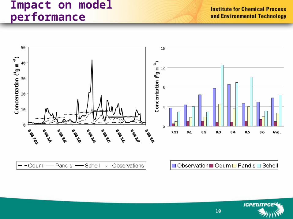
Impact on model performance

0

10

20

30

40

50

0:00 7/31

0:00 8/1

0:00 8/2

0:00 8/3

0:00 8/4

0:00 8/5

0:00 8/6

0:00 8/7

0:00 8/8

Co

nce

ntr

atio

n (m g

m-3

)

PIME3

0

4

8

12

16

7/31 8/1 8/2 8/3 8/4 8/5 8/6 Avg.

Co

nce

ntr

atio

n (m g

m-3

)

PIME3

11

Conclusions and discussion

Schell Pandis Odum

Science best among three simplified not usable

SOA-generation n x Pandis 10n x Odum very low

performance good on average underestimate dramatic

underestimate

Note wide range of norm.bias

Deficiency/problem no partitioning of org. OAY, not

IAY

aerosol to gas phase

overestimate SOA

(corrected in CMAQ 4.3?)

12

Odum algorithm problem: OAY vs. IAY

OAY = Overall AY

= average AY

from ROG=0 and M0=0

to ROG= ROG* and M0=M0*

IAY = Instantaneous AY

= AY at ROG* and M0*

R O G

M 0

S lo p e = IA Y

S lo p e = OAY

R O G *0

M 0*

1

2

13

OAY equation vs. IAY equation

i i

ii

MK

KMOAY

0om,

om,0 1

α

i i

ii

i i

ii

MK

K

MK

K

IAY

20om,

2om,

2

0om,

om,

1

α

1

α

edMcM

baMIAY

0

20

20 )(

.αα

,αα2

,αα

,αα

,αα

22om,2

21om,1

2om,21om,12om,1om,

22om,

21om,21

2om,21om,1

2om,1om,21

KKe

KKKKd

KKc

KKb

KKa

• Jiang (2003), Atmos. Environ. (in press)

14

OAY or IAY: A big deal?

0 .1 1 1 0 1 0 0 1 ,0 0 0M 0 (mg /m 3)

0 .0 0

0 .0 4

0 .0 8

0 .1 2

0 .1 6

0 .2 0

Aer

osol

Yie

ld

1 0

1 0 0

1 ,0 0 0

1 0 ,0 0 0

1 0 0 ,0 0 0

% D

iffe

renc

e

A n th ro p o g en ic

IAY

OAY

IAY - OAY 100 OAY

0 .1 1 1 0 1 0 0 1 ,0 0 0M 0 (mg /m 3)

0 .0 0

0 .1 0

0 .2 0

0 .3 0

0 .4 0

Aer

osol

Yie

ld

1 0 0

1 ,0 0 0

1 0 ,0 0 0

% D

iffe

renc

e

B io g en ic

IAY - OAY 100 OAY

IAY

OAY

Yes, a big deal both conceptually and quantitatively.

15

Acknowledgment

• US EPA: Original Models–3/CMAQ

• Environment Canada Pollution Data Branch, Air Quality Research Branch, Pacific & Yukon Region:

Raw emissions and ambient measurement data

• Dr. D. G. Steyn of the University of British Columbia: Pacific ’93 data set

• Program of Energy Research and Development (PERD) in Canada:

Funding support

16

Thank you !