comparison of two approaches to modeling...
TRANSCRIPT

Ždímal et al., Aerosol and Air Quality Research, Vol. 8, No. 4, pp. 392-410, 2008
Comparison of Two Approaches to Modeling Atmospheric Aerosol Particle Size Distributions
Vladimír Ždímal1*, Marek Brabec2,3, Zden k Wagner4
1 Laboratory of Aerosol Chemistry and Physics, Institute of Chemical Process Fundamentals of the AS CR, v. v. i., Rozvojová 135, Praha 6, 165 02, Czech Republic
2 Department of Biostatistics and Informatics, National Institute of Public Health, Šrobárova 48, Praha 10, 100 42
3 Department of Nonlinear Modeling, Institute of Computer Science, Pod Vodárenskou v ží 2, Praha 8, 182 07, Czech Republic
4 E. Hála Laboratory of Thermodynamics, Institute of Chemical Process Fundamentals of the AS CR, v. v. i., Rozvojová 135, Praha 6, 165 02, Czech Republic
Abstract
This paper compares two approaches to modeling (smoothing) aerosol particle size distribution (particle counts for specified diameter intervals): i) the semiparametric approach based on a maximum likelihood fitting of lognormal (LN) mixtures at each time separately, followed by smoothing parameter tracks, ii) the nonparametric approach based on a kernel-like smoothing as an application of the gnostic theory of uncertain data. The specific advantages and disadvantages of both the semiparametric and nonparametric approaches are discussed and illustrated using real data containing a day-long time series of size spectra measurements.
Keywords: Particle size distribution; Lognormal mixture; Semiparametric modeling; Nonparametric modeling; Gnostic theory of uncertain data.
INTRODUCTION various perspectives. There are many potential approaches that differ in the level of sophistication, computational load, preliminary information requirements, or assumptions needed to justify them. However, we can think of two basic classes into which they can be categorized: nonparametric and semiparametric models.
The data describing the dynamics of particle size distribution (PSD) are inevitably complex and might be modeled statistically from
*Corresponding author: Fax: +420-220920661,
Tel: +420-220390246
E-mail address: [email protected]
392

Ždímal et al., Aerosol and Air Quality Research, Vol. 8, No. 4, pp. 392-410, 2008
The semiparametric models of our interest consist of two parts. The parametric part postulates a mathematical formula to describe PSD feasibly and uses it, together with the measurement error distribution specification, to fit the PSD at each measurement time (e. g., by maximum likelihood). The time dynamics of parameters are then smoothed nonparametrically. The model specification involves assumptions that always behave as a two-edged sword: they can improve efficiency if they are approximately correct, but can spoil the analysis if they are not plausible. In real data fitting, such a model cannot have too many parameters and will not follow every little detail of the data. Rather, it should be able to capture the most important features and skip the minor ones, in line with the philosophy embodied in the aphorism by George E. P. Box (Box and Draper, 1987): “All models are wrong. But some of them are useful.” On the other hand, nonparametric models try to escape the danger of possibly incorrect parametric model specifications by making as few assumptions as possible. Typically, only very basic notions are employed, mainly the smoothness of the fitted distribution. The resulting solution then makes a compromise between the quality of the fit and its smoothness. Such an approach is certainly appealing since it creates the impression that it represents a sort of ideal, fool-proof or automatic tool that does not require any substantial assumption-making and hence precludes preliminary thinking about model choice. Unfortunately, nothing is for free and the impression is not correct for several reasons.
Generally, the efficiency is less important (the approximately correct parsimonious parametric model can estimate things in a more efficient and stable way). More influential is the fact that the balance between smoothness and the goodness-of-fit is not easy to establish. A wrong setting of procedural details can easily lead to over/underfitting, which is usually not substantial for the overall performance of the smoother, but can be disastrous for the fit of the local details of substantial interest (e. g., local maxima size and location). When focusing on these details, special techniques and/or a lot of fine tuning might be required (Marron and Chaudhuri, 1998) that are not easy to implement for large spectral time series data, or a lot of personal experience with similar data is required (as well as some subjective judgment).
In this work we discuss the semi- and nonparametric model properties and illustrate their capabilities on the data from a real measurement campaign. As a representative of the semiparametric methodology we used a lognormal (LN) mixture for the description of the PSD, followed by a loess nonparametric smoother (to smooth the parameter dynamics). LN mixtures were selected because mixtures with few lognormal components (1, 2 or 3) have traditionally been used in aerosol research both for theoretical computations (Seinfeld and Pandis, 1998) and for practical data analysis (Makela et al., 2000; Voutilainen and Kaipio, 2002). We chose a flexible gnostic smoother as a representative of purely nonparametric methods. It was used as an example of a technique that is similar to traditional kernel smoothing methods, but enjoys robustness and
393

Ždímal et al., Aerosol and Air Quality Research, Vol. 8, No. 4, pp. 392-410, 2008
interesting motivation built on first principles (Kovanic, 1986). Its scale parameter, which defines the bandwidth, is estimated in such a way that the entropy of the original data is equal to the entropy of the calculated distribution function. The smoothness of the gnostic distribution function is thus determined by the data adopting the rule “let the data speak for themselves.”
In this text, we will try to compare both approaches to show their weak and strong points. We will stress namely those features that the potential user should be aware of.
MATERIAL AND MEASUREMENT METHODS
We analyzed data obtained from one day of a
measurement campaign that took place at the
Finokalia Station on the island of Crete, Greece
as a part of the EC-funded 5th FP project called
SUB-AERO (Lazaridis et al., 2006). The
chosen subset of data was obtained using a
Scanning Mobility Particle Sizer (SMPS,
Model 3934, TSI Inc., USA). This aerosol
spectrometer consists of two major parts. In the
Electrostatic Classifier (Model EC 3071A),
one narrow fraction of particles having the
same electrical mobility is selected. This
fraction then enters the Condensation Particle
Counter (CPC 3022A) where particles grow by
the condensation of n-butanol on their surface
and are counted optically. The field strength in
the EC changes continuously in order to scan
the whole available mobility range. After the
scan is completed, a sophisticated program
provides the aerosol number size distribution in
the sample. In this experiment, each scan lasted
for 90 seconds and was followed immediately
by another scan. The data matrix has 953T
spectra, measured on January 12, 2001 in
equidistant time intervals (1.5 minutes apart)
from 00:00:10 to 23:59:59. Each scan went
through 103 mobility/size channels. At the -th
time we got a measurement of the cumulative
particle count ( ), meaning the count of
particles with a diameter smaller than or equal
to the i -th size limit, (i.e., the count in the
interval
t
itN
id
0
0 3nmd
, id d ) , where 1 2i
7 2 and the boundaries increased
exponentially, 1i id d with 1 0367 ,
103I . Consequently, the measured diameter
range spanned the interval 7 23 294 2 nm.
SEMIPARAMETRIC MODEL—LOGNORMAL MIXTURES
The PSD is modeled parametrically (as an LN mixture), separately at each measurement time. The mixture parameters are estimated via maximum likelihood. These rough estimates of the time tracks are then smoothed nonparametrically to obtain a clearer picture of trends and more or less local systematic changes in their values.
ModelThe parametric model of the size distribution
at time 1t t can be formulated as:
394
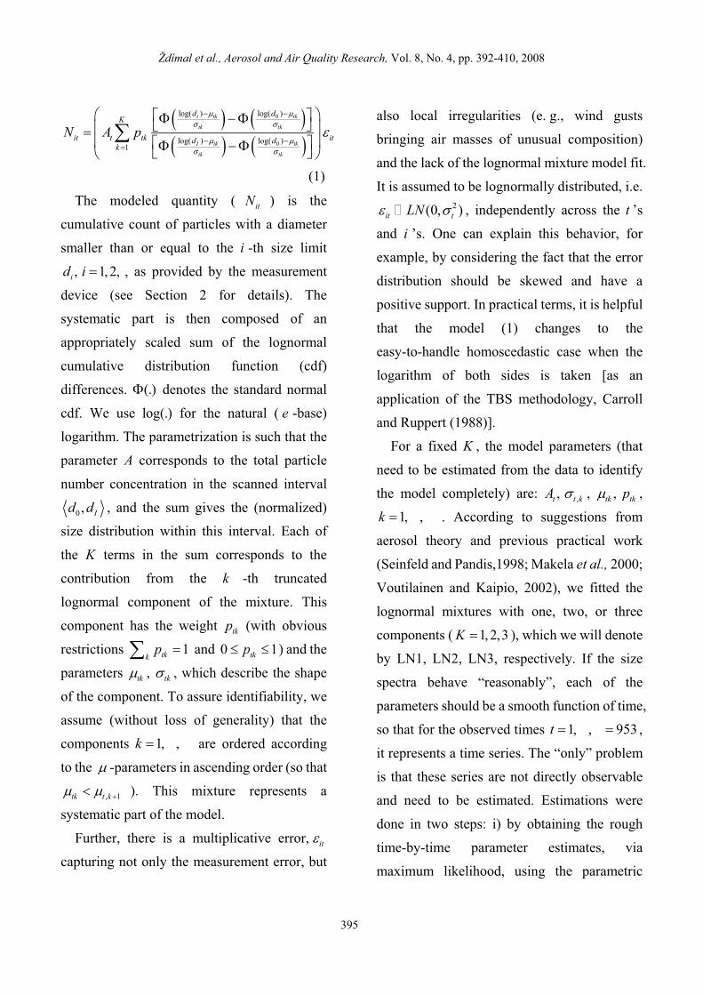
Ždímal et al., Aerosol and Air Quality Research, Vol. 8, No. 4, pp. 392-410, 2008
0
0
log( ) log( )
log( ) log( )1
i tk tk
tk tk
I tk tk
tk tk
d dK
it t tk itd dk
N A p
(1)
The modeled quantity ( ) is the
cumulative count of particles with a diameter
smaller than or equal to the i -th size limit
, as provided by the measurement
device (see Section 2 for details). The
systematic part is then composed of an
appropriately scaled sum of the lognormal
cumulative distribution function (cdf)
differences. denotes the standard normal
cdf. We use lo for the natural ( -base)
logarithm. The parametrization is such that the
parameter
itN
1 2id i
( )
g( ) e
A corresponds to the total particle
number concentration in the scanned interval
0 Id d , and the sum gives the (normalized)
size distribution within this interval. Each of
the terms in the sum corresponds to the
contribution from the k -th truncated
lognormal component of the mixture. This
component has the weight
K
tkp (with obvious
restrictions and ) and the
parameters
1tkkp
tk
0 1tkp
, tk , which describe the shape
of the component. To assure identifiability, we
assume (without loss of generality) that the
components are ordered according
to the
1k
-parameters in ascending order (so that
1tk t k ). This mixture represents a
systematic part of the model.
Further, there is a multiplicative error, it
capturing not only the measurement error, but
also local irregularities (e. g., wind gusts
bringing air masses of unusual composition)
and the lack of the lognormal mixture model fit.
It is assumed to be lognormally distributed, i.e. 2(0 )it tLN
i
, independently across the t ’s
and ’s. One can explain this behavior, for
example, by considering the fact that the error
distribution should be skewed and have a
positive support. In practical terms, it is helpful
that the model (1) changes to the
easy-to-handle homoscedastic case when the
logarithm of both sides is taken [as an
application of the TBS methodology, Carroll
and Ruppert (1988)].
For a fixed K , the model parameters (that
need to be estimated from the data to identify
the model completely) are: ,t tA tkpk , tk ,
1 ,k
K
. According to suggestions from
aerosol theory and previous practical work
(Seinfeld and Pandis,1998; Makela et al., 2000;
Voutilainen and Kaipio, 2002), we fitted the
lognormal mixtures with one, two, or three
components ( 1 2 3 ), which we will denote
by LN1, LN2, LN3, respectively. If the size
spectra behave “reasonably”, each of the
parameters should be a smooth function of time,
so that for the observed times t ,
it represents a time series. The “only” problem
is that these series are not directly observable
and need to be estimated. Estimations were
done in two steps: i) by obtaining the rough
time-by-time parameter estimates, via
maximum likelihood, using the parametric
1 , 953
395

Ždímal et al., Aerosol and Air Quality Research, Vol. 8, No. 4, pp. 392-410, 2008
Estimation model (1) and the implied likelihood function,
and: ii) by smoothing the parameter time-tracks
via a flexible nonparametric smoother loess
(Cleveland and Devlin, 1988). The two steps
represent a semi-parametric approach (the size
distribution is modeled parametrically, the time
dynamics nonparametrically), in an attempt to
combine the useful properties of both. The
basic idea is that the available knowledge about
the distributional shape should be used to
improve the efficiency and restrict the
distributional shape range to exclude wild
shapes that might be otherwise suggested by
the count distortion introduced; e. g., by the
measurement error. On the other hand, very
little is known about the time-dynamics of the
spectra a priori, so that the time evolution
should be specified as flexibly as possible.
Model (1) can be fitted relatively easily via maximum likelihood for each time t and a fixed . From a practical point of view, all that is required is the numerical maximization of the logarithm of the likelihood. We used quasi-Newton-Raphson here. Log likelihood behaves in a relatively decent way, as long as is not large (which was our case with
K
K1 K 3 choices). For numerical and substantive reasons, we reparametrized the component proportions tkp ’s via a cumulative logit transformation (Agresti, 1990), so that obvious tkp s properties were automatically enforced.
Convergence was generally good when we
used the following scheme to construct the
(time-dependent) starting values. For LN1 we
started from the observed count in 0 Id d for
the initial A estimate, with the average and
standard deviation of logarithms of the class
interval centers (weighted by the
time-averaged particle count observed in the
particular class) for and . For LN2, we
started from the LN1 results and added an
additional component, whose location was
suggested by the analysis of the residuals after
the LN model. For LN3, we started from the
LN2.
Let us consider one of the tasks typical for aerosol spectra analysis, namely the search for the number and location of distributional modes. In the LN mixture model, the number of peaks arises as a consequence of the parameter configuration. It is important to note that it is always less than or equal to the number of LN components. This is because some components can be wide enough and located closely enough so that they blend together into one peak. In this sense, the parametric model is much more informative than the plain smoothing of observed counts. It can discover components drifting apart before they are distant enough to be visible on the surface.
For a given , we estimated the parameter tracks (i.e., smoothed them) by the robust variant of the loess smoother (Cleveland and Devlin, 1988). As it is quadratic only locally, its shape is allowed to change with time, so that the resulting track estimate is generally highly
K
396
Ždímal et al., Aerosol and Air Quality Research, Vol. 8, No. 4, pp. 392-410, 2008
Although one might see the time-varying as a realistic feature, the time-dynamics smoothing becomes much more complicated with the parameter space dimension changes. Even though there are elegant Bayesian approaches to this (Green, 1995), they tend to be quite complicated and computationally demanding even in much simpler set-ups than we encounter here. Therefore, we employed two simpler approaches. The first was to use the results of the largest model considered (LN3) and to smooth its parameters in a straightforward way. Admittedly, this might lead to occasional overfitting (when a less parsimonious model would be chosen by the selection procedure) and hence, a somewhat inefficient parameter estimation. Nevertheless, the extent of the problems should not be typically too large for two reasons: the parameter values are smoothed anyway, so that occasional excesses related to unstable estimation should be suppressed (as long as the LN3 model is approximately valid most of the time), and one is often not interested directly in the parameters but in their functions (like location and/or size of the peaks of the size spectra) which are much more stable than the parameters themselves.
tKnonlinear. The smooth fit represents a compromise between a perfect (but rough and inefficient) fit and smoothness. The “exchange rate” in this compromise is given by the span parameter. The span gives a proportion of the data that are used locally to estimate the value at a particular time (a larger span means more smoothness). We chose a span from 0.1-0.25 (after some experimentation and inspection of the quality and smoothness of the fit). The tracks were smoothed for each parameter separately. To get the ˆ tA estimate, we smoothed the logs of the original time-specific MLEs and exponentiated the results. The swere obtained via renormalization of the smoothed estimates (so that they add to one, as they should). The other parameters were smoothed directly.
ˆ tkp
In the previous text, we proceeded as if Kwas known. Obviously, in practice K is not known and must be selected somehow. Since we restricted the values of K to 1 3 and hence fitted lognormal mixtures with one, two and three components, we had to select one of them. To this end, we used a (crude) procedure mimicking the likelihood ratio test at the level of 0.10 [to alleviate the possible problems with the parameter space boundary (McCulloch and Searle, 2001)]. The decision scheme was as follows: i) if the test of LN2 vs. LN1 was not significant, we selected LN1, ii) if the test in i) was significant, we conducted a test of LN3 vs. LN2 and selected LN3 or LN2 when it was/was not significant, respectively. Clearly, such a procedure generally leads to a time-varying number of lognormal component’s estimates ( ).
K
tK
When the interest is predominantly in peak location dynamics, our second approach can be utilized—that is time-by-time testing can be applied to select (time-varying) the dimensionality estimate , then peak locations can be smoothed instead of parameters.
tK
All the computations were done in S-plus (Venables and Ripley, 1994). For the
397

Ždímal et al., Aerosol and Air Quality Research, Vol. 8, No. 4, pp. 392-410, 2008
Results of the Semiparametric Model minimization of the negative log likelihood, we used the built-in function nlminb. A two-stage estimation (estimating the LN parameters time-by-time and then smoothing the estimates by a nonparametric smoother like loess) is just one way to get to the resulting estimates. It is certainly not the most efficient way, but it offers a relatively easily usable tool for processing masses of data. It is potentially more efficient to build time smoothing into the model explicitly; e. g., by postulating a time series model in parameters [e. g., in multivariate ARIMA style, or even more elegantly in a state-space framework, (Voutilainen and Kaipio, 2001)]. This is appealing from both the theoretical and the statistical point of view, but the approach certainly presents two obstacles: i) the computational complexity, ii) the need for a reasonable dynamic statistical model specification. We did not go to the development of the time series model (which would be rather specific for the Crete space-time location), because of not having enough aerosol-dynamics-related information on hand to be able to build such a model, and wanting to demonstrate mainly the difference between the totally nonparametric (section 4) and the more specific semiparametric modeling approaches, while simultaneously staying relatively general (so that the finding can be applied mode widely). One possible consequence might be that we lost some efficiency that the more-specific model could probably have gained. Nevertheless, we do not expect that the time series specification would increase the efficiency dramatically.
When processing the real data, we replaced the occasional zero observed counts in the first several intervals by small numbers (by halves of the minimum nonzero count observed in that particular interval during the observed period). Since the spectrum for the first observed time ( 1t ) was rather aberrant, we excluded it from further analyses (and proceeded with a relabeled time index, running from 1 ,( 1)t ). Fig. 1 compares the results of the LME fit of LN1, LN2 and LN3 to the size spectrum obtained on January 12, 2001 at 00:42:09. The open circles correspond to
( )o g ( )
dd
N
ltd N
d estimated internally by the
measurement device at the size interval midpoints (by taking the derivatives of ssmoothed internally by the measurement device); i.e., to the quantities that we did notuse for fitting. We used a raw (empirical) cumulative count instead to avoid the arbitrary pre-smoothing step and the arbitrary placement to the interval midpoint where only the total interval count is available. As a consequence, the open circles and lines are only approximately comparable.
itN
t
The plot illustrates how the fit improves as we go from LN1 (which is forced to have one peak only, so that it tries to do its best by fitting the main peak and then seriously distorting the lower and upper end of the distribution), to LN2 (which still misses the lower peak even though it can theoretically fit two peaks—because both available components are spent to describe the complicated main peak shape) and LN3 (which picks both peaks fairly
398

Ždímal et al., Aerosol and Air Quality Research, Vol. 8, No. 4, pp. 392-410, 2008
well, while smoothing the peak densities a little bit due to the inherent measurement variability). Note also that the fitted lines correspond to median responses and not to their expected values (the two are quite different quantities under the lognormal distribution of it ’s in 1).
Fig. 2 illustrates the dynamics of the fitted
total particle number concentrations ( A s) in
the monitored diameter interval 0d dI ,
estimated from the LN3 model. is measured
in hours (0-24) and corresponds to the actual
measurement time. Fig. 2(a) shows the
situation after smoothing implied by the
nonparametric part of the model, while 2(b)
shows results of time-by-time LN3 estimation
without any smoothing of parameters along the
time line.
Fig. 1. The fits of a particle size distribution obtained on January 12, 2001 at 00:42:09 by the semiparametric model with one, two and three LN components (lines), compared with the data (points).
Fig 3. LN3, the smoothed time tracks of the
1 2 3ˆ? estimates.
Fig. 3 compares the smoothed estimates of
the 1 2 3k k parameters. Notice that the
smoothed estimates respect the 1? k k
restriction (as they should). 1ˆ tends to
remain low and pretty stable over time. There
are much more dynamics in 2 3
ˆ k
behavior.
All three components show a quite abrupt
change of the behavior close to 11 a.m. Even
this observation alone might offer interesting
insights into the aerosol size distribution
evolution. Notice however, that s
Fig. 2. The time track of the total particle number concentration A estimated using the LN3 model. Dots represent the measured points in both cases; the curve represents the LN3 model fit: a) after smoothing, and b) before smoothing with the loess smoother.
399

Ždímal et al., Aerosol and Air Quality Research, Vol. 8, No. 4, pp. 392-410, 2008
obviously do not represent estimates of the
spectrum peak locations on the log scale. In
fact, there can easily be a smaller number of
peaks than 3 even if the fitted LN3 is
non-trivial. This is because the peak locations
depend in a complicated way on relative
location of ˆ k
k,
2ˆ
s as well as on other parameters.
We will discuss peak locations later.
From comparison, we can see that in
terms of particle count it is representative, the
first component is rather “small.” Nevertheless,
its behavior might be of utmost interest (e.g., in
connection with the nucleation mode
development). The (almost) inverse relation
between
p
p and 3p is obviously given by
the sum-to-one restriction (and the fact that the
1p is small). The other possible smoothing strategy
mentioned in the section Estimation is to fit LN1, LN2, LN3 and to decide for one of them by an LRT-like testing, compute local maxima for the selected mixture and finally smooth the local maxima. One would expect that this approach should lead to more parsimonious time-dependent K . The potential gains in efficiency (achieved by sparing a few parameters) might be offset by: i) the random nature of the selection procedure (the test necessarily commits both type I and type II errors), ii) occasional jumps in maxima locations before smoothing (induced by dimensionality ( K ) changes), and hence it is not entirely clear whether it really pays off to go with the more difficult-to-handle model. The percentages of times when LN1, LN2 or
LN3 was selected by the test-based procedure were 6.4 %, 18.9% and 74.7 %, respectively. In other words, the LN3 prevails (so that the previous approach with always fitting LN3 should not be too bad); but the percentage of the simpler mixtures is not totally negligible—providing some motivation for time-varying K attempts. Not only that the improvement provided by going from LN2- LN3 is not always the same, but also that it is distributed unevenly along the time axis. Greatest improvements occur around 11 and 15 hours.
Fig. 4. The locations of non-smoothed local maxima on particle distribution functions and their evolution in time (as determined by the semiparametric model).
When we take all the smoothed parameters together, we can easily use them to derive other quantities of practical interest. The position of local maximum might be one of them. Many others can be computed just as easily; for example, local maxima sizes. But even subtler ones, like the locations of maxima of the first derivative of the spectral density, can be computed as well. When we selected one of the
400

Ždímal et al., Aerosol and Air Quality Research, Vol. 8, No. 4, pp. 392-410, 2008
fitted models by the testing procedure described earlier and found the local peaks (numerically), we plotted their rough (not-smoothed) peak locations in Fig. 4. Specifically, the number of peaks is not forced to be 3 (in fact, it varies between 1, 2 and 3). Resulting local maxima of the regression function are plotted separately for each time. The proportions of the times when one, two or three peaks were found in the fitted are 18.9%, 43.1%, 37.9%, respectively. Note also that even this relatively easy procedure clearly visualized modal changes occurring in the late morning (around 11 a. m.). These changes are connected to a complicated transitional phenomenon, so called “particle formation event” (see also section Results of the Nonparametric Model), which is sometimes observed in atmospheric aerosol sampling campaigns. It is not the aim of this paper to deal with its mechanism in detail. However, a widely accepted explanation says that there are some thermodynamically stable clusters (TSC) present in the atmosphere. As the size of these clusters is under the lower detection limits of most aerosol spectrometers, they are practically “invisible.” Under favorable conditions, e. g. when a sufficient amount of condensable vapors is available in the atmosphere, these vapors condense on the cluster's surface causing its growth. When the cluster becomes visible for the spectrometer, it is detected. On the measured spectra, it looks like a new mode coming from the lowest sizes and increasing with time. Various parameters may then be extracted from its time behavior; e. g., the growth rate, production rate of the
condensable vapor, and so on (Kulmala et al.,2004).
NONPARAMETRIC MODEL
The PSD is modeled by means of tools taken from the gnostic theory of uncertain data developed by Kovanic (1986). Over the years of development, the gnostic theory has grown into a set of tools, each of which finds its application in some branch of data analysis. The tools differ in the kind of robustness. Tools taking advantage of the quantifying distribution function possess the robustness with respect to inliers (outer robustness) and are useful for signal processing and similar applications.
The opposite case; i.e., the robustness with respect to outliers (inner robustness) is a feature of the tools based upon estimating distribution functions. Two kinds of estimating distribution functions are available, a global and a local one.
The global estimating distribution function is by definition unimodal. It can be used to verify the homogeneity of a data sample or to describe properties of such a sample. However, the PSD of atmospheric aerosols is usually multimodal, the global estimating distribution function thus cannot be used. The local estimating distribution function is a kernel estimate and can therefore describe multimodal distributions. In the following text, we will use the local estimating distribution function only.
401

Ždímal et al., Aerosol and Air Quality Research, Vol. 8, No. 4, pp. 392-410, 2008
Summary of the gnostic theory of uncertain data
In this section we summarize the most important features of the gnostic theory of uncertain data. We limit explanation to the local estimating distribution function. This work extends the methodology of using the local estimating distribution function so that the optimal bounds of a finite data support can be estimated. This will be explained in the section Data Support
The modeled quantity is the number of particles of the particular size class. We will model both variations of the particle number in the time domain, as well as the PSD at a specific time. The equations will therefore be given in an abstract way and both types of usage will be explained later.
The first axiom of the gnostic theory states that the measured value can be expressed as a sum of an ideal value , which is the mathematical model of the true value, and uncertainty, which is a product of a scale parameter and normalized uncertainty
a
0a
S :
0a a S (2)
Using transformations
0 0exp( ) exp( )z a z a (3)
a multiplicative model is obtained:
1 10 exp( )S Sz z (4)
Since conversion between the additive and the multiplicative model is straightforward, all
the following equations will be written for the multiplicative model only.
The basic properties are defined for each individual observation and the equations have been derived by Kovanic (1986) from the above-mentioned axiom. Having the observation z , we can calculate the probability of an ideal value being less or equal to :0z
01( )
2hp z (5)
where h is irrelevance defined as
2 2
2 2
11
q qhq q
(6)
and1
0
Szqz
(7)
After substituting z and into Eq. (5) and differentiating, we get the density
0z
22 2
0 0 0
4log
S Sdp z z
d z S z z (8)
It can be proven that Eq. (8) satisfies all conditions required for Parzen’s kernels (Parzen, 1962). The shape of the kernel is determined by the value of the scale parameter. If , the kernel converges to a 0S
-function. Entropy can be calculated both for the data sample , and the smoothed kernel estimate. We will select such value of which yields equal entropy in both cases. The value of the scale parameter is thus
kz 1k
S
402
Ždímal et al., Aerosol and Air Quality Research, Vol. 8, No. 4, pp. 392-410, 2008
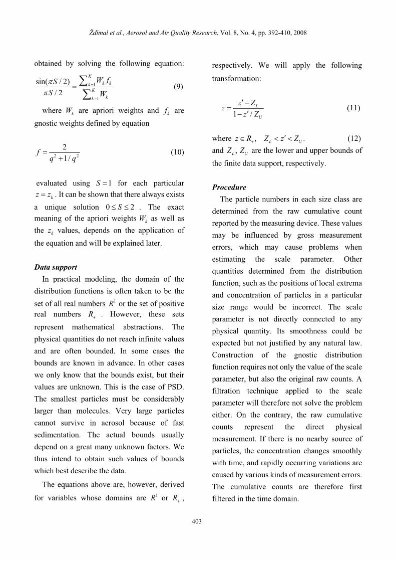
obtained by solving the following equation:
1
1
sin( 2)2
Kk kk
Kkk
W fSS W
(9)
where are apriori weights and kW kf are gnostic weights defined by equation
2
21
fq q2
2
(10)
evaluated using for each particular . It can be shown that there always exists
a unique solution 0 . The exact meaning of the apriori weights as well as the values, depends on the application of the equation and will be explained later.
1S
kz z
kz
S
kW
Data support In practical modeling, the domain of the
distribution functions is often taken to be the set of all real numbers 1R or the set of positive real numbers R . However, these sets represent mathematical abstractions. The physical quantities do not reach infinite values and are often bounded. In some cases the bounds are known in advance. In other cases we only know that the bounds exist, but their values are unknown. This is the case of PSD. The smallest particles must be considerably larger than molecules. Very large particles cannot survive in aerosol because of fast sedimentation. The actual bounds usually depend on a great many unknown factors. We thus intend to obtain such values of bounds which best describe the data.
The equations above are, however, derived
for variables whose domains are 1R or R ,
respectively. We will apply the following
transformation:
1L
U
z Zzz Z
(11)
where Lz R Z z ZU (12) and L UZ Z are the lower and upper bounds of the finite data support, respectively.
ProcedureThe particle numbers in each size class are
determined from the raw cumulative count reported by the measuring device. These values may be influenced by gross measurement errors, which may cause problems when estimating the scale parameter. Other quantities determined from the distribution function, such as the positions of local extrema and concentration of particles in a particular size range would be incorrect. The scale parameter is not directly connected to any physical quantity. Its smoothness could be expected but not justified by any natural law. Construction of the gnostic distribution function requires not only the value of the scale parameter, but also the original raw counts. A filtration technique applied to the scale parameter will therefore not solve the problem either. On the contrary, the raw cumulative counts represent the direct physical measurement. If there is no nearby source of particles, the concentration changes smoothly with time, and rapidly occurring variations are caused by various kinds of measurement errors. The cumulative counts are therefore first filtered in the time domain.
403
Ždímal et al., Aerosol and Air Quality Research, Vol. 8, No. 4, pp. 392-410, 2008
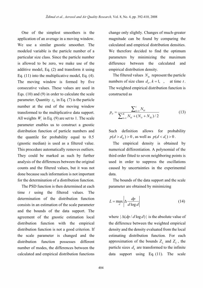
One of the simplest smoothers is the application of an average in a moving window. We use a similar gnostic smoother. The modeled variable is the particle number of a particular size class. Since the particle number is allowed to be zero, we make use of the additive model, Eq. (2) and transform it using Eq. (11) into the multiplicative model, Eq. (4). The moving window is formed by five consecutive values. These values are used in Eqs. (10) and (9) in order to calculate the scale parameter. Quantity in Eq. (7) is the particle number at the end of the moving window transformed to the multiplicative data support. All weights in Eq. (9) are set to 1. The scale parameter enables us to construct a gnostic distribution function of particle numbers and the quantile for probability equal to 0
0z
iW
5(gnostic median) is used as a filtered value. This procedure automatically removes outliers. They could be marked as such by further analysis of the differences between the original counts and the filtered values, but it was not done because such information is not important for the determination of a distribution function.
The PSD function is then determined at each time using the filtered values. The determination of the distribution function consists in an estimation of the scale parameter and the bounds of the data support. The agreement of the gnostic estimation local distribution function with the empirical distribution function is not a good criterion. If the scale parameter is changed and the distribution function possesses different number of modes, the differences between the calculated and empirical distribution functions
change only slightly. Changes of much-greater magnitude can be found by comparing the calculated and empirical distribution densities. We therefore decided to find the optimum parameters by minimizing the maximum difference between the calculated and empirical distribution density.
t
The filtered values represent the particle numbers of size class at time t .The weighted empirical distribution function is constructed as
ktN
kd k 1
1
11( )
iktk
it Kkt t Ktk
Np
N N N 2 (13)
Such definition allows for probability , as well as .( )Kp d d 0 01( )p d d
The empirical density is obtained by numerical differentiation. A polynomial of the third order fitted to seven neighboring points is used in order to suppress the oscillations caused by uncertainties in the experimental data.
The bounds of the data support and the scale parameter are obtained by minimizing
maxlogd
dpLd d
(14)
where ( logdp d d ) is the absolute value of the difference between the weighted empirical density and the density evaluated from the local estimating distribution function. For each approximation of the bounds LZ and UZ , the particle sizes are transformed to the infinite data support using Eq. (11). The scale
kd
404
Ždímal et al., Aerosol and Air Quality Research, Vol. 8, No. 4, pp. 392-410, 2008
parameter is calculated from Eq. (9). The filtered particle numbers are used in place of the apriori weights and the gnostic weights
ktN
kW
kf are evaluated from the particle sizes transformed into the infinite data support. Variable required in Eq. (10) is the weighted median, the definition of which is given in the following paragraph.
0z
iLet p , be the probabilities defined by the weighted empirical distribution function, Eq. (13). Let be a given value such that
1i
N
P1p P p . Then let rp be the greatest
value satisfying rp P and sp be the least value satisfying sP . The quantile for probability is defined as a value obtained by inverse linear interpolation using
pP
rp and sp .The weighted median is defined as the weighted quantile for .0 5P
The definition does not allow for an evaluation of the weighted quantiles for 1P pand . We must be able to calculate weighted quantiles before the bounds of the data support are determined. Extrapolation below and above the experimental data is therefore impossible.
NpP
Before the weighted median can be used in Eq. (10), it must be converted into the infinite data support by means of Eq. (11).
The objective function, Eq. (14) may possess several local minima. In order to determine the global minimum, the generalized random search with alternating heuristics (GCRS/ALTH) developed by Tvrdík et al. is used (Krivý and Tvrdík, 1995; Tvrdík and Krivý, 1999; Tvrdík et al., 2001). The MatLab implementation of the algorithm is available from the author’s website (Tvrdík) and the
function can also be used with Octave (Octave).
For mostly numerical reasons Eq. (11) is not used directly. We first normalize the values of particle diameters:
log( )exp 2 1log( )
min
max min
d dzd d
(15)
where and are the minimum, and
maximum values of the particle diameter d
and
mind maxd
z is the normalized multiplicative value
such that 1 e z e
6 1 1
. We now find optimum
values of the bounds in the normalized data
support. The GCRS/ALTH algorithm requires
limits of the box type. The limits, such as
10 LZ e
Ld
and , are wide
enough so that the optimum value is not missed.
Bounds and are then evaluated from
Eq. (15).
1 1 610Ue Z
Ud
The LZ - UZ space extends over 12 orders of magnitude and is asymmetric. Its metrics prefers LZ close to data and UZ distant from data. We therefore perform minimization for transformed values:
1 16
1 1 6 6 1 1
log( )log( 10 )2 1 2log( 10 ) log(10 )
ULL U
Z eZX Xe e
1
(16)
Results of the Nonparametric Model The gnostic filter applied to the time series
of particle counts is very simple. We prefer a fast response to the quality of filtration. The main purpose is removal of measurements that are evidently wrong and replacing them by a
405

Ždímal et al., Aerosol and Air Quality Research, Vol. 8, No. 4, pp. 392-410, 2008
smoothed value. Filter performance is presented in Fig. 5. You can see that the line corresponding to the filtered values slightly reduces the scatter of the experimental data while following the main trend of the time series. Two outliers were removed.
Fig. 5. Example: the time series of the concentration of particles in the size bin 109.4 nm; the measured values (points) and a smoothed line estimated by the gnostic filter.
Fig. 6. A fit of a particle size distribution obtained on January 12, 2001 at 00:42:09 by the nonparametric model (line), compared with the time-filtered data (points).
In this work we used only a distribution function with a constant scale parameter where
needed in Eq. (10) is obtained as a weighted median converted to the infinite data support. The typical distribution is depicted in Fig. 6. It can be seen that small peaks were smoothed out.
0z
Fig. 7. The distribution density function (curve) determined by the gnostic method. Experimental data are denoted by points. The sample contains a relatively high concentration of small particles.
The character of the distribution is changed in the period from 11 h to 16 h during a particle formation event that has already been discussed in the section Results of the Semiparametric Model. The concentration of small particles is increased, and they often form two separate local maxima. Such a distribution is depicted in Fig. 7.
COMPARISON
Parametric modeling offers an excellent tool if the model is in agreement with the real data. If the model is based upon theoretical assumptions, the parameters estimated from the data provide a useful insight, which can
406

Ždímal et al., Aerosol and Air Quality Research, Vol. 8, No. 4, pp. 392-410, 2008
help in understanding phenomena occurring in the atmosphere. The method, however, fails if the data depart considerably from the model.
The gnostic approach presents a nonparametric method. The value of the scale parameter does not depend on the analyst, it is determined from the condition of entropy equality and thus the risk of under- or over-smoothing is relatively low. The use of the finite data support improves agreement between the empirical and gnostic distribution functions at the edges of the size interval. The number of local maxima is then obtained from an analysis of the distribution function.
The comparison of the original data and its fit by a semiparametric and a nonparametric method are shown in Figs. 1 and 6. The semiparametric method is represented by 3 curves, corresponding to the LN1, LN2 and LN3 models. It can be seen that in this case both LN3 and the nonparametric model describe the measured data reasonably well, recovering both the main peak at 60 nm and also the small one below 10 nm.
Figs. 4 and 8 then show how the two approaches succeeded in capturing the positions of local maxima on the particle distributions’ densities as they move in time during the analyzed day. Again, both methods behaved similarly. It seems, however, that the nonparametric approach yielded a more robust result (the positions of local maxima do not change that much with time). The reason is obvious: the nonparametric method performed data filtration in the time domain at first, and it removed a lot of noise from the data. Both approaches revealed the particle formation
event starting around 11 a.m., both followed the growth of these particles until the evening when the concentration maxima connected to these particles disappeared. However, as this new maximum was superimposed on a distribution that already had 3 other maxima, the LN3 model naturally failed to describe the fourth one.
Fig. 8. The locations of local maxima on particle distribution functions and their evolution in time (as determined by the nonparametric model).
Fig. 9. The concentration of particles with a size below 30nm and the total concentration of particles.
407

Ždímal et al., Aerosol and Air Quality Research, Vol. 8, No. 4, pp. 392-410, 2008
Fig. 9 reveals that within the mentioned time period the aerosol is formed mostly by the newly appearing small particles with sizes below 30 nm. Since this local maximum dominates the distributions, the maxima at other sizes are sometimes changed into shoulders on another peak. This causes short gaps in Fig. 8.
Another important difference is found when calculating the concentration of particles. Let’s assume that there are two sources, each of which produces particles with lognormal size distributions. Parametric approach gives us the concentrations for each source of particles. Such information is not available if the nonparametric approach is used. It is only possible to find a local minimum between the two modes and evaluate the concentrations of the particles with sizes lower and greater than the size at the minimum.
A related issue is that of information compression. The parametric model with a few LN components compresses the empirical information into a compact form—parameter estimates. Consider for instance the “compression ratio”—that is the reciprocal of the ratio between the number of datapoints in the empirical spectra (number of channels) and the number of parameters in the LN mixture that is used to fit them. For our data, it is
for LN3 and it is obviously even better for simpler mixtures. The nonparametric methodology can offer compression if we are interested only in the number and positions of modes. If we later need some other type of information, we either have to repeat the calculation, or the calculated
parameters must be stored in addition to the measured data. This is the price paid for higher flexibility in nonparametric estimates.
9 103 0 0874
CONCLUSIONS
This paper presents two methods of modeling atmospheric PSDs: the parametric approach and the nonparametric. Our general view is that in this comparison there is no absolute winner; both approaches have their merits. However, in order to give our kind reader some hints, we will try to summarize pros and cons of both approaches.
The semiparametric method based on lognormal mixtures has these advantages: a) it is more efficient and less computationally demanding; b) it gives excellent results if the model agrees with the data; c) it provides a high data compression ratio; d) it gives concentration of aerosol particles corresponding to each of the modes; and f) it is more easily programmable since its lognormal components are available as built-in functions in most statistical packages.
The drawbacks of the semiparametric method are: a) if the data depart considerably from model assumptions, the method fails to arrive at correct and physically sound results, but this fact may not be recognized from the results itself; b) the method becomes more complicated when the number of LN distributions in the mixture (K) changes with time; and c) it does not follow fast changes in the PSDs well even if number K is kept constant (but that depends more on the
408
Ždímal et al., Aerosol and Air Quality Research, Vol. 8, No. 4, pp. 392-410, 2008
REFERENCESnonparametric smoothing of parameter tracks than on the LN parametric part).
Agresti, A. (1990). Categorical Data Analysis.John Wiley, New York.
The nonparametric method based on the gnostic theory of uncertain data offers these advantages: a) the method is based on fewer assumptions and does not force the data to have any particular shape; b) it keeps the amount of information contained in the data by fulfilling the condition of preserving the entropy; c) the method is robust to outliers; d) it follows fast changes in the PSD; e) it provides good agreement with the data even at the edges of the PSD.
Box, G.E. and Draper, N.R. (1987). EmpiricalModel-Building and Response Surfaces.John Wiley, New York.
Carroll, R.J. and Ruppert, D. (1988). Transformation and Weighting in Regression. Chapman and Hall, London.
Cleveland, W.S. and Devlin, S.J. (1988). Locally-Weighted Regression: An Approach to Regression Analysis by Local Fitting. J. Am. Statist. Assoc. 83: 596–610. The main disadvantages of this method are: a)
it is not directly available in the statistical packages and so it has to be programmed; b) it is more computationally demanding because the use of a reliable global nonlinear optimization algorithm is inevitable; c) it does not compress the data, even if it provides practically important results as integral concentrations in a given size range or number and position of distributional modes.
Green, P.J. (1995). Reversible Jump Markov chain Monte Carlo Computation and Bayesian Model Determination. Biometrika,82: 711–732.
Kovanic, P. (1986). A New Theoretical and Algorithmical Basis for Estimation, Identification and Control. Automatica. 22: 657–674.
Krivý, I. and Tvrdík, J. (1995). The Controlled Random Search Algorithm in Optimizing of Regression Models. Comp. Stat. & Data Analysis. 20: 229–234.
ACKNOWLEDGEMENTS
This work was supported by these grants of the EC: ENVK2-1999-00052 and EUSAAR contract RII3-CT-2006-026140, by Czech Science Foundation grant No. 205/03/1560, and partly by the Institutional Research Plan AV0Z10300504 “Computer Science for the Information Society: Models, Algorithms, Applications.”
Kulmala, M., Vehkamaäki, H., Petaäjaä, T., Dal Maso, M., Lauri, A., Kerminen, V.-M., Birmili, W. and McMurry, P. H. (2004). Formation and Growth Rates of Ultrafine Atmospheric Particles: A Review of Observations. J. Aerosol Sci. 35: 143–176.
Lazaridis, M., Eleftheriadis, K., Smolik, J., Colbeck, I., Kallos, G., Drossinos, Y., Zdimal, V., Vecera, Z., Mihalopoulos, N., Mikuska, P., Bryant, C., Housiadas, C., Spyridaki, A., Astitha, M. and Havranek, V.
409

Ždímal et al., Aerosol and Air Quality Research, Vol. 8, No. 4, pp. 392-410, 2008
410
(2006). Dynamics of Fine Particles and Photo-Oxidants in the Eastern Mediterranean (SUB-AERO). Atmos.Environ. 40: 6214–6228.
Lee, C.-K., Lin, S.-C. (2008) Chaos in Air Pollutant Concentration (APC) Time Series. Aerosol Air Qual. Res. 8: 381-391.
Makela, J.M., Koponen, I.K., Aalto, P. and Kulmala, M. (2000). One-year Data of Submicron Size Modes of Tropospheric Background Aerosol in Southern Finland. J. Aerosol Sci. 31: 595–611.
Marron, J.S. and Chaudhuri, P. (1998). When is a Feature Really There? The SiZer Approach. In Sadjadi, F. A., Editor, Autom. Target Recognition VII, Proc. of SPIE, 3371: 306–312.
McCulloch, C.E. and Searle, S.R. (2001). Generalized, Linear, and Mixed Models.John Wiley, New York.
Octave. URL http://www.octave.org. Parzen, E. (1962). On Estimation of a
Probability Density Function and Mode. Ann.Math. Statist. 33: 1065–1076.
Seinfeld, J.H. and Pandis, S.N., 1998. Atmos.Chem. and Physics. J. Wiley & Sons, New York.
Tvrdík, J. URL http://albert.osu.cz/tvrdik/. Tvrdík, J. and Krivý, I. (1999). Simple
Evolutionary Heuristics for Global Optimization. Computational Statistics and Data Analysis, 30: 345–352.
Tvrdík, J., Krivý, I. and Misík, L. (2001). Evolutionary Algorithm with Competing Heuristics. In Proceedings of Mendel 2001.pages 58–64. VUT Brno, 2001. Also available from http://albert.osu.cz/tvrdik/index_pic_en.html.
Venables, W.N. and Ripley, B.D. (1994). Modern Applied Statistics with S-Plus.Springer, New York.
Voutilainen, A. and Kaipio, J.P. (2002). Estimation of Time-Varying Aerosol Size Distributions—Exploitation of Modal Aerosol Dynamical Models. J. Aerosol Sci.33: 1181–1200.
Voutilainen, A. and Kaipio, J.P. (2001). Estiation of Non-Stationary Aerosol Size Distributions Using the State-Space Approach. J. Aerosol Sci. 32: 631–648.
Received for review, July 21, 2008 Accepted, November 5, 2008