Complexity vs. Performance: Empirical Analysis of MachineLearning as a Service

Yuanshun Yaoysyao@cs.uchicago.eduUniversity of Chicago

Zhujun Xiaozhujunxiao@cs.uchicago.edu

University of Chicago

Bolun Wangbolunwang@cs.ucsb.edu

UCSB/University of Chicago

Bimal Viswanathviswanath@cs.uchicago.edu

University of Chicago

Haitao Zhenghtzheng@cs.uchicago.eduUniversity of Chicago

Ben Y. Zhaoravenben@cs.uchicago.edu

University of Chicago

ABSTRACTMachine learning classifiers are basic research tools used in numer-ous types of network analysis and modeling. To reduce the need fordomain expertise and costs of running local ML classifiers, networkresearchers can instead rely on centralized Machine Learning as aService (MLaaS) platforms.

In this paper, we evaluate the effectiveness of MLaaS systemsranging from fully-automated, turnkey systems to fully-customizablesystems, and find that with more user control comes greater risk.Good decisions produce even higher performance, and poor deci-sions result in harsher performance penalties. We also find thatserver side optimizations help fully-automated systems outperformdefault settings on competitors, but still lag far behind well-tunedMLaaS systemswhich compare favorably to standaloneML libraries.Finally, we find classifier choice is the dominating factor in deter-mining model performance, and that users can approximate theperformance of an optimal classifier choice by experimenting witha small subset of random classifiers. While network researchersshould approach MLaaS systems with caution, they can achieveresults comparable to standalone classifiers if they have sufficientinsight into key decisions like classifiers and feature selection.

CCS CONCEPTS• Computing methodologies→Machine learning; • Appliedcomputing;

1 INTRODUCTIONMachine learning (ML) classifiers are now common tools for dataanalysis. They have become particularly indispensable in the con-text of networking, where characterizing the behavior of protocols,services, and users often requires large scale data mining andmodel-ing. ML tools have pervaded problems from all facets of networking,

Permission to make digital or hard copies of all or part of this work for personal orclassroom use is granted without fee provided that copies are not made or distributedfor profit or commercial advantage and that copies bear this notice and the full citationon the first page. Copyrights for components of this work owned by others than ACMmust be honored. Abstracting with credit is permitted. To copy otherwise, or republish,to post on servers or to redistribute to lists, requires prior specific permission and/or afee. Request permissions from permissions@acm.org.IMC ’17, November 1–3, 2017, London, United Kingdom© 2017 Association for Computing Machinery.ACM ISBN 978-1-4503-5118-8/17/11. . . $15.00https://doi.org/10.1145/3131365.3131372

with examples ranging from network link prediction [43, 54], net-work localization [41, 77], user behavior analysis [71, 72], conges-tion control protocols [59, 74], performance characterization [8, 76],botnet detection [31], and network management [1].

As ML tools are increasingly commoditized, most network re-searchers are interested in them as black box tools, and lack theresources to optimize their deployments and configurations ofML systems. Without domain experts or instructions on buildingcustom-tailoredML systems, some have tried developing automatedor “turnkey” ML systems for network diagnosis [42]. A more ma-ture alternative is ML as a Service (MLaaS), with offerings fromGoogle, Amazon, Microsoft and others. These services run on thecloud, and provide a query interface to an ML classifier trainedon uploaded datasets. They simplify the process of running MLsystems by abstracting away challenges in data storage, classifiertraining, and classification.

Given the myriad of decisions in designing any ML system, it isfitting that MLaaS systems cover the full spectrum between extremesimplicity (turn-key, nonparametric solutions) and full customiz-ability (fully tunable systems for optimal performance). Some aresimple black-box systems that do not even reveal the classifier used,while others offer users choice in everything from data preprocess-ing, classifier selection, feature selection, to parameter tuning.

MLaaS today are opaque systems, with little known about theirefficacy (in terms of prediction accuracy), their underlying mecha-nisms and relative merits. For example, howmuch freedom and con-figurability do they give to users?What is the difference in potentialperformance between fully configurable and turnkey, “black-box”systems? Can MLaaS providers build in better optimizations thatoutperform hand-tuned user configurations? Do MLaaS systemsoffer enough configurability to match or surpass the performanceof locally tuned ML tools?

In this paper, we offer a first look at empirically quantifyingthe performance of 6 of the most popular MLaaS platforms acrossa large number (119) of labeled datasets for binary classification.Our goals are three-fold. First, we seek to understand how MLaaSsystems compare in performance against each other, and against afully customized and tuned local ML library. Our results will shedlight on the cost-benefit tradeoff of relying on MLaaS systems in-stead of locally managing ML systems. Second, we wish to betterunderstand the correlations between complexity, performance andperformance variability. Our results will not only help users choosebetween MLaaS providers based on their needs, but also guide com-panies in traversing the complexity and performance tradeoff when

Preprocessing Feature

Selection

Classi ier

Choice

Parameter

Tuning

Program

Implementation

Trained

Model

ABM

Google

Amazon

PredictionIO

BigML

Microsoft

Training

Data

Query

Data

Prediction

Results

Figure 1: Standard ML pipeline and the steps that can be controlled by different MLaaS platforms.

building their own local ML systems. Third, we want to understandwhich key knobs have the biggest impact on performance, and tryto design generalized techniques to optimize those knobs.

Our analysis produces a number of interesting findings.

• First, we observe that current MLaaS systems cover the full rangeof tradeoffs between ease of use and user-control. Our resultsshow a clear and strong correlation between increasing config-urability (user control) and both higher optimal performance andhigher performance variance.• Second, we show that classifier choice accounts for much ofthe benefits of customization, and that a user can achieve near-optimal results by experimenting with a small random set ofclassifiers, thus dramatically reducing the complexity of classifierselection.• Finally, our efforts find clear evidence that fully automated (black-box) systems like Google and ABM are using server-side teststo automate classifier choices, including differentiating betweenlinear and non-linear classifiers. We note that their mechanismsoccasionally err and choose suboptimal classifiers. As a whole,this helps them outperform other MLaaS systems using defaultsettings, but they still lag far behind tuned versions of theircompetitors. Most notably, a heavily tuned version of the mostcustomizable MLaaS system (Microsoft) produces performancenearly-identical to our locally tuned ML library (scikit-learn).

To the best of our knowledge, this paper is the first effort toempirically quantify the performance of MLaaS systems. We believeMLaaS systems will be an important tool for network data analysisin the future, and hope our work will lead to more transparencyand better understanding of their suitability for different networkresearch tasks.

2 UNDERSTANDING MLAAS PLATFORMSMLaaS platforms are cloud-based systems that provide machinelearning as a web service to users interested in training, building,and deploying ML models. Users typically complete an ML taskthrough a web page interface. These platforms simplify and makeML accessible to even non-experts. Another selling point is theaffordability and scalability, as these services inherit the strengthsof the underlying cloud infrastructure.

For our analysis, we choose 6 mainstream MLaaS platforms, in-cluding Amazon Machine Learning (Amazon1), Automatic Business

1https://aws.amazon.com/machine-learning

Modeler (ABM2), BigML3, Google Prediction API (Google4), Mi-crosoft Azure ML Studio (Microsoft5), and PredictionIO6. These arethe MLaaS services widely available today.The MLaaS Pipeline. Figure 1 shows the well-known sequenceof steps typically taken when using any user-managed ML software.For a given ML task, a user first preprocesses the data, and identifiesthe most important features for the task. Next, she chooses an MLmodel (e.g. a classifier for a predictive task) and an appropriate im-plementation of the model (since implementation difference couldcause performance variation [9]), tunes parameters of the modeland then trains the model. Specific MLaaS platforms can simplifythis pipeline by only exposing a subset of the steps to the userwhile automatically managing the remaining steps. Figure 1 alsoshows the steps exposed to users by each platform. Note that some(ABM and Google) expose none of the steps to the user but providea “1-click” mode that trains a predictive model using an uploadeddataset. At the other end of the spectrum, Microsoft provides controlfor nearly every step in the pipeline.Control and Complexity. It is intuitive that more control overeach step in the pipeline allows knowledgeable users to build higherquality models. Feature, model, and parameter selection can havesignificant impact on the performance of anML task (e.g. prediction).However, successfully optimizing each step requires overcomingsignificant complexity that is difficult without in-depth knowledgeand experience. On the other hand, when limiting control, it isunclear whether services can perform effective automatic man-agement of the pipeline and parameters, e.g. in the case of ABMand Google. Current MLaaS systems cover the whole gamut interms of user control and complexity and provide an opportunityto investigate the impact of complexity on performance.

We summarize the controls available in the pipeline for classifica-tion tasks in each platform. More details are available in Section 3.• Preprocessing: The first step involves dataset processing. Com-mon preprocessing tasks include data cleaning and data trans-formation. Data cleaning typically involves handling missingfeature values, removing outliers, removing incorrect or dupli-cate records. None of the 6 systems provides any support forautomatic data cleaning and expects the uploaded data to bealready sanitized with errors removed. Data transformation usu-ally involves normalizing or scaling feature values to lie within

2http://e-abm.com3https://bigml.com4https://cloud.google.com/prediction5https://azure.microsoft.com/en-us/services/machine-learning6http://predictionio.incubator.apache.org

Control

Pe

rfo

rma

nce

a

nd

Ris

k

MoreLess

Lo

wH

igh

GoogleABM

Amazon

BigMLPredictionIO

Microsoft

Local

Figure 2: Overview of control vs. performance/risk tradeoffsin MLaaS platform.

certain ranges. This is particularly useful when features lie indifferent ranges, where it becomes harder to compare variationsin feature values that lie in a large range with those that lie ina smaller range. Microsoft is the only platform that providessupport for data transformation.• Feature selection: This step selects a subset of features most rel-evant to the ML task, e.g. those that provide more predictivepower for the task. Feature selection helps improve classificationperformance, and also simplifies the problem by eliminating ir-relevant features. A popular type of feature selection scheme isFilter method, where a statistical measure (independent of theclassifier choice) is used to rank features based on their classdiscriminatory power. Only Microsoft supports feature selectionand provides 8 Filter methods. Some platforms, e.g. BigML, pro-vide user-contributed scripts for feature selection. We excludethese cases since they are not officially supported by the platformand require extra effort to integrate them into the ML pipeline.• Classifier selection: Different classifiers can be chosen based onthe complexity of the dataset. An important complexity measureis the linearity (or non-linearity) of the dataset, and classifierscan be chosen based on their capability of estimating a linear ornon-linear decision boundary. Across all platforms, we experi-ment with 10 classifiers. ABM and Google offer no user choices.Amazon only supports Logistic Regression7. BigML provides 4classifiers, PredictionIO provides 8, while Microsoft gives thelargest number of choices: 9.• Parameter tuning: These are parameters associated with a clas-sifier and they must be tuned for each dataset to build a highquality model. Amazon, PredictionIO, BigML, and Microsoft allsupport parameter tuning. Usually each classifier allows users totune 3 to 5 parameters. We include detailed information aboutclassifiers and their parameters in Section 3.

Key Questions. To help understand the relationships betweencomplexity, performance, and transparency in MLaaS platforms,

7Amazon does not specify which classifier is used during the model training, butthis information is claimed in its documentation page: http://docs.aws.amazon.com/machine-learning/latest/dg/types-of-ml-models.html.

we focus our analysis around three key questions and briefly sum-marize our findings. Figure 2 provides a simple visualization to aidour discussion.

• How does the complexity (or control) of ML systems correlate withideal model accuracy? Assuming we cover the available config-uration space, how strongly do constraints in complexity limitmodel accuracy in practice? How do different controls comparein relative impact on accuracy?Answer : Our results show a clear and strong correlation betweenincreasing complexity (user control) and higher optimal per-formance. Highly tunable platforms like Microsoft outperformothers when configurations of the ML model are carefully tuned.Among the three control dimensions we investigate, classifierchoice accounts for the most benefits of customization.• Can increased control lead to higher risks (of building a poorlyperforming ML model)? Real users are unlikely to fully optimizeeach step of the ML pipeline. We quantify the likely performancevariation at different levels of user control. For instance, howmuch would a poor decision in classifier cost the user in practiceon real classification tasks?Answer: We find higher configurability leads to higher risks ofproducing poorly performing models. The highest levels of per-formance variation also come from choices in classifiers. We alsofind that users only need to explore a small random subset ofclassifiers (3 classifiers) to achieve near-optimal performanceinstead of experimenting with an entire classifier collection.• How much can MLaaS systems optimize the automated portionsof their pipeline? Despite their nature as black boxes, we seekto shed light on hidden optimizations at the classifier level inABM and Google. Are they optimizing classifiers for differentdatasets? Do these internal optimizations lead to better perfor-mance compared to other MLaaS platforms?Answer: We find evidence that black-box platforms, i.e. Googleand ABM, are making a choice between linear and non-linearclassifiers based on characteristics of each dataset. Results showthat this internal optimization successfully improves these plat-forms’ performance, when compared to other MLaaS platforms(Amazon, PredictionIO, BigML andMicrosoft) without tuning anyavailable controls. However, in some datasets, a naive optimiza-tion strategy that we devised makes better classifier decisionsand outperforms them.

3 METHODOLOGYWe focus our efforts on binary classification tasks, since that isone of the most common applications of ML models in deployedsystems. Moreover, binary classification is one of the two learningtasks (the other being regression) that are commonly supportedby all 6 ML platforms. Other learning tasks, e.g. clustering andmulti-class classification, are only supported by a small subset ofplatforms.

3.1 DatasetsWe describe the datasets we used for training ML classifiers. We use119 labeled datasets from diverse application domains such as lifescience, computer games, social science, and finance etc. Figure 3(a)

Lif e Science : 44

Compute r & Games : 18

Synthe tic : 17

Social Science : 10

Physical Science : 10

Financial & Business : 7

N/A : 13

Financial & Business: 7

Other: 13

Physical Science: 10

Social Science: 10

Synthetic: 17Computer & Game: 18

Life Science: 44

(a) Breakdown of application domains.

0

0.2

0.4

0.6

0.8

1

10 100 1k 10k 100k

CD

F o

f D

ata

se

ts

Number of Samples

(b) Distribution of sample numbers.

0

0.2

0.4

0.6

0.8

1

1 10 100 1k 4.7k

CD

F o

f D

ata

se

ts

Number of Features

(c) Distribution of feature numbers.

Figure 3: Basic characteristics of datasets used in our experiments.

shows the detailed breakdown of application domains. The major-ity of datasets (94 out of 119) are from the popular UCI machinelearning repository [3], which is widely adopted for benchmarkingML classifiers. The remainder include 16 popular synthetic datasetsfrom scikit-learn8, and 9 datasets used in other applied machinelearning studies [5, 13, 17, 18, 32, 33, 70, 73]9. It is also importantto highlight that our datasets vary widely in terms of the numberof samples and number of features, as shown in Figure 3(b) andFigure 3(c). Datasets vary in size from 15 samples to 245, 057 sam-ples, while the dimensionality of datasets ranges from 1 to 4, 702.Note that we limit the number of extremely large datasets (with sizeover 100k) due to the high computational complexity incurred inusing them on MLaaS platforms. We include complete informationabout all datasets separately10. As none of the MLaaS platformsprovides any support for data cleaning, we perform the followingdata preprocessing steps locally before uploading to MLaaS plat-forms. Our datasets include both numeric and categorical features.Following prior conventions [23], we convert all categorical fea-tures to numerical values by mapping {C1, ...,CN } to {1, ...,N }. Weacknowledge that this may impact performance of some classifiers,e.g. distance-based classifiers like kNN [45]. But since our goal is tocompare performance across different platforms instead of acrossclassifiers, this preprocessing is unlikely to change our conclusions.For datasets with missing values, we replace missing fields withmedian values of corresponding features, which is a common MLpreprocessing technique [62]. Finally, for each dataset, we randomlysplit data samples into training and test set by 70%–30% ratio. Wetrain classifiers on each MLaaS platforms using the same trainingand held-out test set. We report classification performance on thetest set.

3.2 MLaaS Platform MeasurementsIn this section, we describe our methodology for measuring classi-fication performance of MLaaS platforms when we vary availablecontrols.Choosing Controls of an ML System. As mentioned in Sec-tion 2, we break down an ML system into 5 dimensions of con-trol. In this paper, we consider 4 out of 5 dimensions by excluding

8http://scikit-learn.org9There are two datasets used in [73].10http://sandlab.cs.uchicago.edu/mlaas

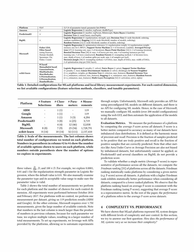
Program Implementation which is not controllable in any plat-form. The remaining dimensions are grouped into three categories,Preprocessing (data transformation) and Feature Selection (FEAT),Classifier Choice (CLF), and Parameter Tuning (PARA). Note thatwe combine Preprocessing with Feature Selection to simplify ouranalysis, as both controls are only available in Microsoft. In therest of the paper, we interchangeably use the term Feature Selec-tion and FEAT to refer to this combined category. Overall, thesethree categories of control present the easiest and most impactfuloptions for users to train and build high quality ML classifiers. Asbaselines for performance comparison, we use two reference pointsthat represent the extremes of the complexity spectrum, one withno user-tunable control, and one where users have full control overall control dimensions. To simulate an ML system with no control,we set a default choice for each control dimension. We refer tothis configuration as baseline in later sections. Since not all ofthe 6 platforms we study have a default classifier, we use LogisticRegression as the baseline, as it is the only classifier supported byall 4 platforms (where the control is available). All MLaaS platformsselect a default set of parameters for Logistic Regression (valuesand parameters vary across platforms), and we use them for thebaseline settings. We perform no feature selection for the baselinesettings. To simulate an ML system with full control, we use a localML library, scikit-learn, as this library allows us to tune all controldimensions. We refer to this configuration as local in later sections.Performing Measurements by Varying Controls. We evalu-ate performance of MLaaS platforms on each dataset by varyingavailable controls. Table 1 provides detailed information about avail-able choices for each control dimension. We vary the FEAT and CLFdimensions by simply applying all available choices listed for eachsystem in Table 1. It is interesting to note that the CLF choicesvary across platforms even though all platforms are competing toprovide the same service, i.e. binary classification. For example,Random Forests and Boosted Decision Tree, best performing classi-fiers based on prior work [14, 15], are only available on Microsoft.The PARA dimension is varied by applying grid search. We exploreall possible options for categorical parameters. For example, weinclude both L1 and L2 in regularization options from Logistic Re-gression. For numerical parameters, we start with the default valueprovided by platforms and scan a range of values that are two ordersof magnitude lower and higher than the default. In other words, foreach numerical parameter with a default value of D, we investigate

Platform FEAT CLF (# of parameter tuned: parameter list (PARA))Amazon × Logistic Regression (3: maxIter, regParam, shuffleType)

PredictionIO ×Logistic Regression (3: maxIter, regParam, fitIntercept), Naive Bayes (1:lambda),Decision Tree (2: numClasses, maxDepth),

BigML ×

Logistic Regression (3: regularization, strength, eps), Decision Tree (3: node threshold, ordering,random candidates), Bagging [11] (3: node threshold, number of models, ordering),Random Forests [12] (3: node threshold, number of models, ordering)

Microsoft

Fisher LDA,Filter-based(using Pearson,Mutual, Kendall,Spearman, Chi,Fisher, Count)

Logistic Regression (4: optimization tolerance, L1 regularization weight, L2 regularization weight,memory size for L-BFGS ), Support Vector Machine (2: # of iterations, Lambda), Averaged Percep-tron [27] (2: learning rate, max. # of iterations), Bayes Point Machine [34] (1: # of training iteration),Boosted Decision Tree [28] (4: max. # of leaves per tree, min. # of training instances per leaf,learning rate, # of trees constructed), Random Forests (5: resampling method, # of decision trees,max. depth of trees, # of random splits per node, min. # of samples per leaf),Decision Jungle [58] (5: resampling method, # of DAGs, max. depth of DAGs, max. width of DAGs,# of optimization step per DAG layer),

scikit-learn

FClassif,MutualInfoClassif,GaussianNorm,MinMaxScaler,MaxAbsScaler,L1Normalization,L2Normalization,StandardScaler

Logistic Regression (3: penalty, C, solver), Naive Bayes (1: prior), Support Vector Machine(3: penalty, C, loss), Linear Discriminant Analysis (2: solver, shrinkage), k-Nearest Neighbor(3: n_neighbors, weights, p), Decision Tree (2: criterion, max_features), Boosted Decision Tree(3: n_estimators, criterion, max_features), Bagging (2: n_estimators, max_features), Random Forests(2: n_estimators, max_features), Multi-Layer Perceptron [52] (3: activation, solver, alpha)

Table 1: Detailed configurations forMLaaS platforms and local librarymeasurement experiments. For each control dimension,we list available configurations (feature selection methods, classifiers, and tunable parameters).

Platform # FeatureSelections

# Class-ifiers

# Para-meters

# Measu-rements

ABM - 1 (1) - 119Google - 1 (1) - 119Amazon - 1 (1) 3 (3) 4,284

PredictionIO - 3 (8) 6 (25) 3,719BigML - 4 (4) 12 (46) 12,838

Microsoft 8 (8) 7 (9) 23 (34) 1,728,791scikit-learn 8 (14) 10 (14) 32 (111) 2,137,410

Table 2: Scale of the measurements. The last column showstotal number of configurations we tested on each platform.Numbers in parenthesis in column#2 to #4 show thenumberof available options shown to users on each platform, whilenumbers outside parenthesis show the number of optionswe explore in experiments.

three values: D100 , D, and 100 × D. For example, we explore 0.0001,

0.01 and 1 for the regularization strength parameter in Logistic Re-gression, where the default value is 0.01. We also manually examinethe parameter type and its acceptable value range to make sure theparameter value is valid.

Table 2 shows the total number of measurements we performfor each platform and the number of choices for each control di-mension. All experiments were performed between October 2016and February 2017. For platforms with no control, we perform onemeasurement per dataset, giving us 119 prediction results (ABMand Google). At the other extreme, Microsoft requires over 1.7Mmeasurements, given the large number of available controls. Notethat numbers in the last column is much larger than the productof numbers in previous columns, because for each parameter wetune, we explore multiple values, resulting in a larger number oftotal measurements. To set up experiments, we leverage web APIsprovided by the platforms, allowing us to automate experiments

through scripts. Unfortunately, Microsoft only provides an API forusing preconfigured ML models on different datasets, and there isno API for configuring ML models. Hence, in the case of Microsoft,we manually configure ML models (over 200 model configurations)using the web GUI, and then automate the application of the modelsto all datasets.EvaluationMetrics. Wemeasure the performance of a platformby computing the average F-score across all datasets. F-score is abetter metric compared to accuracy as many of our datasets haveimbalanced class distributions. It is defined as the harmonic meanof precision and recall. Precision is the fraction of samples predictedto be positive that are truly positive and recall is the fraction ofpositive samples that are correctly predicted. Note that other met-rics like Area Under Curve or Average Precision are also not biasedby imbalanced datasets, but unfortunately cannot be applied, asPredictionIO and several classifiers on BigML do not provide aprediction score.

To validate whether a single metric (Average F-score) is repre-sentative of performance across all the datasets, we compute theFriedman ranking [55] of platforms across all the datasets. Friedmanranking statistically ranks platforms by considering a given metric(e.g. F-score) across all datasets. A platform with a higher Friedmanrank exhibits statistically better performance when considering alldatasets, compared to a lower ranked platform. We observe that theplatform ranking based on average F-score is consistent with theFriedman ranking (using F-score), suggesting that average F-scoreis a representative metric. In the rest of the paper, the performanceof a platform refers to the average F-score across datasets.

4 COMPLEXITY VS. PERFORMANCEWe have shown that MLaaS platforms represent ML system designswith different levels of complexity and user control. In this section,we try to answer our first question: How does the performance ofML systems vary as we increase their complexity?

0.6

0.7

0.8

0.9

1G

oo

gle

AB

M

Am

azo

n

Big

ML

Pre

dic

tio

nIO

Mic

roso

ft

Lo

ca

l

Ave

rag

e F

-sco

re Baseline Optimized

ComplexityLow High

Figure 4: Optimized and baseline performance (F-score) ofplatforms and local library.

0

10

20

30

40

Am

azo

nB

igM

LP

red

ictio

nIO

Mic

roso

ftL

oca

l

Am

azo

nB

igM

LP

red

ictio

nIO

Mic

roso

ftL

oca

l

Am

azo

nB

igM

LP

red

ictio

nIO

Mic

roso

ftL

oca

l

F-s

co

re Im

pro

ve

me

nt (%

)

FeatureSelection

ClassifierSelection

ParameterTuning

No

Da

ta

No

Da

ta

Figure 5: Relative improvement in performance (F-score)over baseline as we tune individual controls (white boxes in-dicate controls not supported).

(a) Baseline performance.

Platform Avg. Fried.Ranking

Avg.F-score

Avg.Accuracy

Avg.Precision

Avg.Recall

Amazon 253.7 0.748 (250.5) 0.850 (269.5) 0.782 (298.0) 0.755 (196.7)Google 267.7 0.706 (261.4) 0.851 (217.7) 0.751 (261.4) 0.711 (330.4)ABM 344.5 0.694 (285.8) 0.833 (366.5) 0.738 (359.3) 0.691 (366.6)BigML 348.1 0.688 (326.8) 0.822 (347.2) 0.741 (335.7) 0.688 (385.6)

PredictionIO 379.5 0.672 (389.2) 0.818 (432.6) 0.682 (387.6) 0.741 (308.9)Local 388.8 0.672 (411.9) 0.832 (401.8) 0.668 (419.4) 0.723 (322.1)

Microsoft 424.3 0.655 (477.3) 0.833 (391.9) 0.715 (370.5) 0.659 (457.6)

(b) Optimized performance.

Platform Avg. Fried.Ranking

Avg.F-score

Avg.Accuracy

Avg.Precision

Avg.Recall

Local 190.1 0.839 (179.4) 0.916 (184.2) 0.984 (201.3) 0.990 (195.5)Microsoft 211.1 0.837 (186.5) 0.914 (190.3) 0.954 (231.3) 0.863 (236.3)

PredictionIO 318.6 0.828 (245.7) 0.886 (238.7) 0.779 (478.4) 0.852 (311.5)BigML 365.9 0.789 (307.5) 0.876 (281.7) 0.880 (287.9) 0.802 (351.4)Amazon 446.7 0.761 (545.3) 0.863 (524.3) 0.826 (398.2) 0.795 (318.9)Google 641.9 0.706 (692.6) 0.853 (606.7) 0.744 (605.5) 0.704 (662.9)ABM 758.8 0.694 (784.3) 0.834 (774.1) 0.735 (747.7) 0.684 (729.1)

Table 3: Baseline and optimized performance of MLaaS platforms. The Friedman ranking of each metric is included in theparenthesis. Lower Friedman ranking indicates consistently higher performance across all datasets.

4.1 Optimized PerformanceFirst we evaluate the optimized performance each MLaaS platformcan achieve by tuning all possible controls provided by the platform,i.e. FEAT, CLF, and PARA. In this process, we train individual modelsfor all possible combinations of the 3 controls (whenever available)and use the best performing model for each dataset. We reportthe average F-score across all datasets for each platform as itsperformance. We refer to these results as optimized. Note thatthe optimized performance is simply the highest performance on

the test set that is obtained by training different models using allavailable configurations. We do not optimize the model on test set.

We also generate the corresponding reference points, i.e. base-line and local. For local, we compute the highest performanceon our local ML library by tuning all 3 control dimensions. Forbaseline, we measure the performance of “fully automated”, zero-control versions of all systems (MLaaS and our local library), byusing the baseline configurations for each platform. As mentionedearlier, these reference points capture performance at two ends ofthe complexity spectrum (no control vs. full control).

Figure 4 shows the optimized average F-score for each MLaaSplatform, together with the optimized results. Platforms are listedon the x-axis based on increasing complexity. We observe a strongcorrelation between system complexity and the optimized classi-fication performance. The platform with highest complexity (Mi-crosoft) shows the highest performance (0.83 average F-score), andperformance decreases as we consider platforms with lower com-plexity/control (Google and ABM), with ABM showing the lowestperformance (0.71 F-score). As expected, the local library outper-forms all MLaaS platforms, as it explores the largest range of modelconfigurations (most feature selections techniques, classifiers, andparameters). Note that the performance difference between localand MLaaS platforms with high complexity is smaller, suggestingthat adding more complexity and control beyond Microsoft bringsdiminishing returns. In addition, when we compare the baselineperformance with the optimized performance for platforms withhigh complexity (Microsoft), the difference is significant, with up to26.7% increase in F-score, further indicating that higher complexityprovides room for more performance improvement. Lastly, the er-ror bars show the standard error of the measured performance, andwe observe that the statistical variation of performance measuresfor different platforms is not large.

For completeness, we include the detailed baseline and optimizedperformance of MLaaS platforms in Table 3. We include F-score, andother 3 metrics, accuracy, precision, and recall. We also computethe Friedman ranking of each metric across datasets [55]. A lowerFriedman ranking indicates consistently higher performance overall datasets. Platforms in both tables are ordered based on averageFriedman ranking over 4 evaluation metrics in ascending order. Wecan see that average F-score is a representative metric, because theranking based on F-score values matches the ranking induced bythe Friedman metric.

4.2 Impact of Individual ControlsWehave shown that higher complexity in the form of more user con-trol contributes to higher optimized performance. Now we break-down the potential performance gains from baseline configurations,and investigate the potential gains contributed by each type ofcontrol. In the collection of tunable controls and design decisions,answering this question would tell us which decisions have themost impact on the final performance. We start by tuning onlyone dimension of control while leaving others at baseline settings.Figure 5 shows the percentage improvement in performance fromthe baseline setting for each platform and control dimension. Notethat Google and ABM are not included in this analysis. In addition,we have 3 platforms (Amazon, BigML, PredictionIO) missing in theFeature Selection column, one (Amazon) missing in the ClassifierSelection column. These are the platforms that do not support tun-ing those respective control dimensions. We observe the largestperformance improvement of 14.6% (averaged across all platforms)when giving users the ability to select specific ML classifiers. In fact,in the case of Microsoft, F-score improves by 22.4% which is thehighest among all platforms when we optimize the classifier choicefor each dataset. After the classifier dimension, feature selectionprovides the next highest improvement in F-score (6.1%) acrossall platforms, followed by the classifier parameter dimension (3.4%

improvement in F-score). The above results show that classifier isthe most important control dimension that significantly impactsthe final performance. To shed light on the general performance ofdifferent classifiers, we analyze classifier performance with defaultparameters and with optimized parameter configurations. Table 4(a)shows the top 4 classifiers when using baseline (default) parameters.It is interesting to note that no single classifier dominates in termsof performance over all the datasets. Table 4(b) shows a similartrend even when we optimize the parameters. This suggests thatwe need a mix of multiple linear (e.g. LR, NB) and non-linear (RF,BST, DT) classifiers to achieve high performance over all datasets.Summary. Our results clearly show that platforms with highercomplexity (more dimensions for user control) achieve better per-formance. Among the 3 key dimensions, classifier choice providesthe largest performance gain. Just by optimizing the classifier alone,we can already achieve close to optimized performance. Overall, Mi-crosoft provides the highest performance across all platforms, anda highly tuned Microsoft model can produce performance identicalto that of a highly-tuned local scikit-learn instance.

5 RISKS OF INCREASING COMPLEXITYOur experiments in Section 4 assumed that users were experts oneach step in the ML pipeline, and were able to exhaustively searchfor the optimal classifier, parameters, and feature selection schemesto maximize performance. For example, for Microsoft, we evaluatedover 17k configurations to determine the configuration with opti-mized performance. In practice, users may have less expertise, andare unlikely to experiment with more than a small set of classifiersor available parameters. Therefore, our second question is: Can in-creased control lead to higher risks (of building poorly performing MLmodels)? To quantify risk of generating poorly performing models,we use performance variation as the metric, and compute variationon each platform as we tune available controls.

5.1 Performance Variation across PlatformsFirst we measure the performance variation of each MLaaS plat-form across a range of system configurations (of CLF, PARA, andFEAT) described in Section 3. For each configuration and platform,we compute average performance across all datasets. Then we iter-ate through all configurations, and obtain a range of performancescores which capture the performance variation. Each configurationwould generate a single point in the range of performance scores.Higher variation means a single poor decision in design could pro-duce a significant performance loss. We plot performance variationresults for each platform in Figure 6. As before, platforms on the x-axis are ordered based on increasing complexity. First, we observe apositive correlation between complexity of an MLaaS platform andhigher performance variation. Among MLaaS platforms, Microsoftshows the largest variation, followed by less complex platformslike PredictionIO and Amazon. For Microsoft, F-score ranges from0.49 to 0.75. Also as expected, our local ML library has the highestperformance variation. The takeaway is that even though morecomplex platforms have the potential to achieve higher perfor-mance, there are higher risks of building a poorly configured (andpoorly performing) ML model.

(a) Ranking of classifiers using baseline parameters

Rank BigML PredictionIO Microsoft Local

1 LR (34.5%) LR (42.9%) BST (50.4%) BST (24.4%)2 RF (26.1%) DT (38.7%) AP (16.8%) KNN (12.6%)3 DT (24.4%) NB (18.5%) BPM (10.9%) DT (10.9%)4 BAG (15.1%) RF (7.6%) RF (10.9%)

(b) Ranking of classifiers using optimized parameters

Rank BigML PredictionIO Microsoft Local

1 RF (32.8%) LR (48.7%) BST (43.7%) MLP (32.8%)2 BAG (30.3%) DT (36.1%) DJ (17.6%) BST (27.7%)3 LR (27.7%) NB (16.0%) AP (16.0%) RF (9.2%)4 DT (9.2%) RF (13.4%) KNN (6.7%)

Table 4: Top four classifiers in each platform using baseline/optimized parameters. Number in parenthesis shows the per-centage of datasets where the corresponding classifier achieved highest performance. LR=Logistic Regression, BST=BoostedDecision Trees, RF=Random Forests, DT=Decision Tree, AP=Average Perceptron, KNN=k-Nearest Neighbor, NB=Naive Bayes,BPM=Bayes Point Machine, BAG=Bagged Trees, MLP=Multi-layer Perceptron, DJ=Decision Jungle.

0

0.2

0.4

0.6

0.8

1

Go

og

le

AB

M

Am

azo

n

Big

ML

Pre

dic

tio

nIO

Mic

roso

ft

Lo

ca

l

Ave

rag

e F

-sco

re

ComplexityLow High

Figure 6: Performance variation in MLaaS platforms whentuning all available controls.

0

0.2

0.4

0.6

0.8

1

Am

azo

nB

igM

LP

red

ictio

nIO

Mic

roso

ftL

oca

l

Am

azo

nB

igM

LP

red

ictio

nIO

Mic

roso

ftL

oca

l

Am

azo

nB

igM

LP

red

ictio

nIO

Mic

roso

ftL

oca

l

Pe

rfo

rma

nce

Va

ria

tio

n FeatureSelection

ClassifierSelection

ParameterTuning

No

Da

ta

No

Da

ta

Figure 7: Performance variation when tuning CLF, PARA andFEAT individually, normalized by overall variation (whiteboxes indicate controls not supported).

5.2 Variation from Tuning Individual ControlsNextwe analyze the contribution of each control dimension towardsthe variation in performance. When we tune a single dimension, wekeep the other controls at their default values set by the platform, i.e.use the baseline settings. Figure 7 shows the portion of performancevariation caused by each control dimension, i.e. a ratio normalizedby the overall variation measured in our previous experiment. Weobserve that classifier choice (CLF) is the largest contributor tovariation in performance. For example, in the case of Microsoftand PredictionIO (both exhibiting large variation), over 80% of thevariation is captured by just tuning CLF. Thus, it is important tonote that even though CLF can provide the largest improvementin performance (Section 4), if not carefully chosen, can lead tosignificant performance degradation. On the other hand, for allplatforms, except Amazon, tuning the PARA dimension results inthe least variation in performance. We are unable to verify thereason for the high variation in the case of Amazon (for PARA), butsuspect it is due to either implementation or default parametersettings.Partial Knowledge about Classifiers. Given the dispropor-tionally large impact classifier choice has on performance and per-formance variation, we want to understand how users can makebetter decisions without exhaustively experimenting over the entire

gamut of ML classifiers. Instead, we simulate a scenario where theuser experiments with (and chooses the best out of) a randomly cho-sen subset of k classifiers from all available classifiers in a platform.We measure the highest F-score possible in each k-classifier subset.Next, we average the highest F-score across all possible subsets ofsize k . Results are shown in Figure 8 with all platforms support-ing classifier selection. We observe a trend of rapidly improvingperformance as users try multiple classifiers. We observe that justtrying a randomly chosen subset of 3 classifiers often achieves per-formance that is close to the optimal found by experimenting withall classifiers. In the case of Microsoft, we observe an F-score of 0.76which is only 5% lower than the F-score we can obtain by tryingall 8 classifiers. Performance variation also decreases significantlyonce a user explores 3 or more classifiers in these platforms.Summary. Our results show that increasing platform complex-ity leads to better performance, but also leads to significant per-formance penalties for poor configuration decisions. Our resultssuggest that much/most of the gains can be achieved by focusingon classifier choice, and that experimenting with a random subsetof 3 classifiers often achieves performance and lowers variationclose to optimal.

0.6

0.7

0.8

0.9

1

0 2 4 6 8 10

Avera

ge F

-score

Number of Classifiers Explored

BigMLPredictionIOMicrosoftLocal

Figure 8: Average performance vs. number of classifiers ex-plored.

6 HIDDEN OPTIMIZATIONSIn the final part of our analysis, we seek to shed light on anyplatform-specific optimizations outside of user-visible configura-tions or controls. More specifically, we focus on understandinghidden optimizations used by fully automated black-box platforms,Google and ABM. These platforms have the most leeway to imple-ment internal optimizations, because their entire ML pipeline isfully automated. In Section 4.1 (Figure 4), we observe that Googleand ABM outperform many other platforms when applying defaultconfigurations. This suggests that their hidden configurations aregenerally better than alternative default settings.

Among the countless potential options for optimization, we fo-cus on a simple yet effective technique: optimizing classifier choicesbased on dataset characteristics [46]. We raise the question: Areblack-box platforms automatically selecting a classifier based on thedataset characteristics? Note that our usage of the phrase “selectinga classifier” should be broadly interpreted as covering differentpossible implementation scenarios (for optimization). For example,optimization can be implemented by switching between distinctclassifier instances, or a single classifier implementation that in-ternally alters decision characteristics depending on the dataset.While our analysis cannot infer such implementation details, weprovide evidence of internal optimization in black-box platforms(Section 6.1). We further quantitatively analyze their optimizationstrategy (Section 6.2), and finally examine the potential for improve-ment (Section 6.3)

6.1 Evidence of Internal OptimizationsWe select two datasets from our collection, a non-linearly-separablesynthetic dataset, which we call CIRCLE11, and a linearly-separablesynthetic dataset, referred to as LINEAR12. Figure 9(a) and Fig-ure 9(b) show visualizations of the two datasets. Both datasets haveonly two features. Given the contrasting characteristics (linearity)

11http://scikit-learn.org/stable/modules/generated/sklearn.datasets.make_circles.html12http://scikit-learn.org/stable/modules/generated/sklearn.datasets.make_classification.html

-1

0

1

2

-1.5 -1 -0.5 0 0.5 1 1.5

Fe

atu

re #

2

Feature #1

Class 0 Class 1

(a) Visualization of CIRCLE.

-6

-3

0

3

6

-3 -2 -1 0 1 2 3

Fe

atu

re #

2

Feature #1

Class 0

Class 1

(b) Visualization of LINEAR.

Figure 9: Visualization of two datasets: synthetic non-linearly-separable dataset (CIRCLE) and synthetic linearly-separable dataset (LINEAR).

Category ClassifiersLinear LR, NB, Linear SVM, LDA

Non-Linear DT, RF, BST, KNN, BAG, MLPTable 5: Assignment of classifiers available on local libraryinto linear vs. non-linear categories.

of the two datasets, our hypothesis is that they would help to dif-ferentiate between linear and non-linear classifier families basedon prediction performance.

We examine Google andABM’s prediction results on CIRCLE andLINEAR to infer their classifier choices. Since we have no ground-truth information here, we resort to analyzing decision boundariesgenerated by the two platforms. The decision boundary is visual-ized by querying and plotting the predicted classes of a 100×100mesh grid. Figure 10(a) and Figure 10(b) illustrate Google’s decisionboundary on CIRCLE and LINEAR, respectively. It is very clear thatGoogle’s decision boundary on CIRCLE forms a circle, indicatingGoogle is using a non-linear classifier, or a non-linear kernel, e.g.RBF kernel [67]. On LINEAR, Google’s decision boundary matches astraight line. It showsGoogle is using a linear classifier. Experimentson ABM also show similar results. Figure 10(c) and Figure 10(d)show the decision boundaries of ABM on CIRCLE and LINEAR,respectively. Thus, both platforms are optimizing and switchingclassifier choices for the two datasets. Additionally, Google’s deci-sion boundary on CIRCLE (circular shape) is different from ABM(rectangular shape), indicating that they selected different non-linear classifiers. Based on the shape of decision boundaries, it islikely that Google used a non-linear kernel based classifier whileABM chose a tree-based classifier.

6.2 Predicting Classifier FamilyIn this section, we present a method to automatically predict theclassifier used by a platform using just two pieces of information—knowledge of the training dataset and prediction results from theplatform. Such a method would help us automatically find instanceswhere a black-box platform would change classifiers depending onthe dataset characteristics.

At a high level, we observe that it is hard to pin-point the spe-cific classifier used by a platform, using just the dataset and theprediction results. This is because prediction results of different

-1

0

1

2

-1.5 -1 -0.5 0 0.5 1 1.5

Fe

atu

re #

2

Feature #1

Class 0 Class 1

(a) Google’s decision boundary on CIRCLE.

-6

-3

0

3

6

-3 -2 -1 0 1 2 3

Fe

atu

re #

2

Feature #1

Class 0

Class 1

(b) Google’s decision boundary on LINEAR.

-1

0

1

2

-1.5 -1 -0.5 0 0.5 1 1.5

Fe

atu

re #

2

Feature #1

Class 0 Class 1

(c) ABM’s decision boundary on CIRCLE.

-6

-3

0

3

6

-3 -2 -1 0 1 2 3

Fe

atu

re #

2

Feature #1

Class 0

Class 1

(d) ABM’s decision boundary on LINEAR.

Figure 10: Decision boundaries generated by Google and ABM on CIRCLE and LINEAR. Both platforms produced linear andnon-linear boundaries for different datasets.

0

0.2

0.4

0.6

0.8

1

0 0.2 0.4 0.6 0.8 1

CD

F o

f E

xperim

ents

F-score

Linear

Non-linear

(a) CIRCLE.

0

0.2

0.4

0.6

0.8

1

0 0.2 0.4 0.6 0.8 1

CD

F o

f E

xperim

ents

F-score

Non-linear

Linear

(b) LINEAR.

Figure 11: Performance of predicting local linear/non-linearclassifier choices on CIRCLE and LINEAR datasets.

0

0.2

0.4

0.6

0.8

1

0 0.2 0.4 0.6 0.8 1C

DF

of

Tra

ine

d

Cla

ssifie

rsValidation F-score

Figure 12: Validation perfor-mance of predicting linear/non-linear classifiers.

-1

0

1

2

-1.5 -1 -0.5 0 0.5 1 1.5

Featu

re #

2

Feature #1

Class 0 Class 1

Figure 13: Amazon’s deci-sion boundary on CIRCLE.

classifiers tend to overlap. However, we find that it is possible toaccurately infer the broad classifier family, more specifically, linearor non-linear classifiers.

Our key insight is that we can control datasets used for the in-ference and thus selectively choose datasets that elicit significantdivergence between prediction results of linear and non-linear clas-sifiers. To give an example, we examine the performance of thelocal library classifiers on the CIRCLE and LINEAR datasets. Wecategorize local classifiers into linear and non-linear families, asshown in Table 5. Figures 11(a) and 11(b) shows the performance(F-score) of the two categories of classifiers on the two datasets. Asexpected, we find that linear and non-linear classifiers produce verydifferent F-scores on the two datasets, regardless of other configu-ration settings. Non-linear classifiers outperform linear classifierswhen on CIRCLE. For LINEAR, linear classifiers outperform non-linear classifiers in many cases. This is because of the noisy natureof the dataset causing non-linear classifiers to overfit, and thereforeproduce lower performance compared to linear classifiers. Next, wepresent our methodology to accurately predict the classifier familyby identifying more datasets that show divergence in predictionresults of linear and non-linear classifiers.Methodology. We build a supervised ML classifier for the pre-diction task. For training the classifier, we use prediction results,and ground-truth of classifier choices from the local library and thethree platforms that allow user control of the classifier dimension(i.e. Microsoft, BigML and PredictionIO). Features used for train-ing include aggregated performance metrics (F-score, precision,recall, accuracy), and the predicted labels. We train one classifierfor each dataset in our collection. Each training sample is one ML

experiment using a single configuration of the ML pipeline (i.e.choices of FEAT, CLF and PARA). Measurements are randomly splitinto training, validation, and test sets. Training and validation setscontain 70% of experiments, and test set contains the remaining30% experiments. We train a Random Forests classifier with 5-foldcross-validation, and pick the best performing classifier based onvalidation performance. Based on prior work, Random Forests isone of the best performing classifiers for supervised binary clas-sification tasks [15, 23]. Figure 12 shows the distribution of cross-validation performance of classifiers trained on all 119 datasets.Not all datasets could differentiate linear and non-linear classifiers.There are 64 datasets that produce classifiers achieving higher than0.95 F-score. In other datasets, classifiers failed to separate linearand non-linear classifiers as they produce similar performance. In-tuitively, we do not expect all datasets to perform well, and one goalof the training process is to identify datasets with high differentiat-ing power. We select the 64 datasets where the trained classifiersachieve high performance (F-score > 0.95) on the validation set. Tofurther test if they would generalize and accurately predict classifierchoices, we apply them on the 30% held-out test set. All trainedclassifiers achieve F-score higher than 0.96. This further proves thatthe chosen classifiers can accurately predict the classifier family.Classifier Choices of Google and ABM. We apply the selected64 trained classifiers (covering 64 datasets) on Google and ABMand predict their classifier choices over linear and non-linear family.Results show Google uses linear classifiers on 39 out of 64 (60.9%)datasets, and non-linear classifiers for the remaining 25 (39.1%)datasets. ABM, on the other hand, uses linear classifiers on 44(68.8%) out of 64 datasets, and non-linear on the remaining 20

(a) Google vs. our naïve strategy.

NaïveGoogle Linear Non-linear

Linear 11 (25.5%) 5 (11.6%)Non-linear 17 (39.5%) 10 (23.26%)

(b) ABM vs. our naïve strategy.

NaïveABM Linear Non-linear

Linear 8 (16.7%) 3 (6.3%)Non-linear 22 (45.8%) 15 (31.3%)

Table 6: Breakdown of datasets based on classifier choicewhen our naïve strategy outperforms black-box platforms.

(31.2%) datasets. If we compare Google and ABM, they pick thesame classifier category on 49 (76.6%) datasets, but disagree onthe remaining 15 (23.4%) datasets. The differences in the classifierchoices could contribute to their overall performance differencein Figure 4. Overall, our results suggest that both platforms makedifferent classifier choices (choosing linear or non-linear family)depending on the dataset.Classifier Choices of Amazon. Recall that Amazon does notreveal any classifier information in their model training interface,but claims to use Logistic Regression on their documentation page.We apply our classifier prediction scheme on Amazon to investi-gate whether they are indeed using a single classifier for all tasks.Interestingly, 10 out of all 64 datasets have over 50% configurationsthat are predicted to be non-linear (the remaining are predicted tobe linear). We also observe that Amazon produces a non-linear deci-sion boundary when applied to the CIRCLE dataset (Figure 13). Wesuspect that Amazon uses non-linear techniques on top of LogisticRegression, e.g. non-linear kernel, or even uses other non-linearclassifiers apart from Logistic Regression.

Unfortunately we are unable to corroborate our findings withthe providers (Google, ABM, and Amazon), as all hidden optimiza-tions are kept confidential and proprietary. However, our predic-tions demonstrate high accuracy in our validation and test datasets(where the underlying configuration is known).

6.3 Impact of Internal OptimizationsPrevious experiments show that black-box platforms successfullychoose classifier families with better performance when applied onthe CIRCLE and LINEAR datasets. On these two datasets, Googleand ABMwould outperform a scheme that does not switch betweenclassifier families. But are their strategies optimized for all otherdatasets? Are there cases where the two platforms make the wrongclassifier choice?

To understand the potential for further improvement, we designa naïve classifier selection strategy using the local library, andcompare its performance with Google and ABM. Our intuition isthat if Google and ABM perform poorly when compared to ournaïve strategy, there is potential for further improvement and we

0

0.2

0.4

0.6

0.8

1

0 0.05 0.1 0.15 0.2 0.25 0.3

CD

F o

f D

ata

sets

Difference in F-score

(a) Google.

0

0.2

0.4

0.6

0.8

1

0 0.1 0.2 0.3 0.4 0.5 0.6

CD

F o

f D

ata

sets

Difference in F-score

(b) ABM.

Figure 14: Performance difference in datasets where naïvestrategy outperforms Google/ABM using different classifierfamily.

can understand the cases where classifier choices (i.e. linear vsnon-linear) are potentially incorrect. We choose two widely usedlinear and non-linear classifiers, Logistic Regression and DecisionTree. These two classifiers are supported by most other platforms(Table 1). For each dataset, we train both classifiers and choose theone with higher performance. To further simplify the strategy andto avoid any impact of optimization from other control dimensions,we use the default parameter settings in Logistic Regression andDecision Tree, and perform no feature selection.

For our analysis, we again use the 64 datasets that can accuratelypredict choices of linear and non-linear classifiers. In 43 out of 64datasets, our naïve strategy outperforms Google, and in 48 datasets,it outperforms ABM. This clearly indicates that Google and ABMhave scope for further improvement.

We further compare the choices made by naïve strategy andblack-box platforms. Table 6 shows the breakdown of the datasetsby decisions when naïve strategy outperforms Google and ABM. Inboth platforms, in a majority of cases, the classifier choices do notmatch our simple strategy. In these cases, Google and ABM couldincrease their performance (F-score) by 20% and 34% on average,respectively, by choosing the other classifier family. Figure 14 showsa detailed breakdown (as a CDF) of performance difference betweenthe black-box platforms and naïve strategy, when we outperformthem. The potential performance improvement is significant inmany cases.When is switching classifier the best option for improvement?Although we show the potential performance improvement byswitching classifiers, black-box platforms could use other meth-ods to improve performance. For example, Google and ABM couldperform better parameter tuning and feature selection to reducethe performance gap and justify their classifier choices. To identifycases where classifier switching is likely the best option, we com-pare our naïve strategy with the optimal performance of the otherclassifier family (i.e. not chosen). This means that when naïve strat-egy chooses a non-linear classifier, we compare its performancewith the optimal linear classifier (across all configurations). If naïvestrategy could still outperform Google and ABM under this sce-nario, it indicates that switching the classifier is likely the best wayto further improve the performance. We find 3 datasets in the caseof Google, and 4 for ABM, where changing the classifier is probablythe best option to further improve performance. While our analysis

is limited to the 64 datasets where we can perform prediction, ourfinding highlights the existence of scenarios where Google andABM clearly need to make better classifier choices.

7 RELATEDWORKAnalyzing MLaaS Platforms. There is very limited prior workfocusing on MLaaS platforms. Chan, et al. and Ribeiro, et al. pre-sented two different architecture designs of MLaaS platforms [16,51]. Although we cannot confirm that these architectures are beingused by any of the MLaaS platforms we studied, they shed lighton potential ways MLaaS platforms operate internally. Other re-searchers investigated vulnerabilities of these platforms towardsdifferent types of attacks. This includes attacks that try to leak in-formation about individual training records of a model [26, 57], andthose aiming to duplicate the functionality of a black-box MLaaSmodel by querying the model [64]. While these studies are in gen-eral orthogonal to ourwork, there is scope for borrowing techniquesfrom them that can help us better understand MLaaS platforms.Empirical Analysis of ML Classifiers. Prior empirical analy-sis focused on determining the best classifier for a variety of MLproblems using user-managed ML tools (e.g. Weka, R, Matlab) on alarge number of datasets. Multiple studies conducted an exhaustiveperformance evaluation of up to 179 supervised classifiers usingup to 121 datasets [15, 23, 66]. All studies observe that RandomForests, Boosted or Bagging Trees outperform other classifiers, in-cluding SVM, Naïve Bayes, Logistic Regression, Decision Tree, andMulti-layer Perceptron. Caruana et al. further studied classifier per-formance focusing on high-dimensional datasets [14]. They findthat Random Forests perform better than Boosted Trees on high-dimensional data, and the relative performance difference betweenclassifiers change as dimensionality increases. Other work also fo-cused on evaluating performance of specific classifier families, forexample tree-based classifiers [47, 50], rule-based classifiers [50],and ensemble methods [49].

In comparison, our work does not focus on a single step of theML pipeline. Instead, we analyze end-to-end impact of complexityon classifier performance, through the lens of deployed MLaaSplatforms. This allows us to understand how specific changes to theML task pipeline impact actual performance in a real world system.Instead of focusing only on the best achievable performance forany classifier, we recognize the wide-spread use of ML by generalistusers, and study the “cost” of suboptimal decisions in choosing andconfiguring classifiers in terms of degraded performance.Automated Machine Learning. Many works focused on re-ducing human effort in ML system design by automating classifierselection and parameter tuning. Researchers proposed mechanismsto recommend classifier choices based on classifiers that are knownto perform well on similar datasets [40]. Many mechanisms evenuse machine learning algorithms like collaborative filtering andk-nearest neighbor to recommend classifiers [4, 10, 60]. To performautomatic parameter optimization, methods have been proposedbased on intuition-based Random Search [6, 7], and Bayesian op-timization [7, 25, 37, 61]. These mechanisms have been shown toestimate suitable parameters with less computational complexitythan brute-force methods like Grid Search [21]. Other works pro-posed techniques to automate the entire ML pipeline. For example,

Auto-Weka [39, 63] and Auto-Sklearn [24] could search throughthe joint space of classifiers and their respective parameter settingsand choose the optimal configuration.Experimental Design for Evaluating ML Classifiers. TheML community has a long history on classifier evaluation usingcarefully designed benchmark tests [38, 53, 68]. Many studies pro-posed theoretical frameworks and guidelines for designing bench-mark experiments [22, 36]. Dietterich used statistical tests to com-pare classifiers [20] and the methodology was later improved infollow-up work [19, 29]. Our performance evaluation using Fried-man ranking is based on their methodology. Other work focusedon comparing and benchmarking performance of popular ML soft-ware [30, 69], e.g. Weka [75], PRTools [65], KEEL [2] and, morerecently, deep learning tools [56]. In addition, work has been doneto identify and quantify the relationship between classifier perfor-mance and dataset properties [35, 46], especially dataset complex-ity [44, 48, 78]. Our work leverages similar insights about datasetcomplexity (linearity) to automatically identify classifier familiesbased on prediction results.

8 LIMITATIONSWe point out three limitations of our study. First, we focus on 6mainstream MLaaS platforms, covering services provided by bothtraditional Internet giants (Google, Microsoft, Amazon) and emerg-ing startups (ABM. BigML, PredictionIO). We did not study othercommercial MLaaS platforms because they either focus on highlyspecialized tasks (e.g. image/text classification), or does not supportlarge scale measurements (e.g. posing strict rate limit). Second, wefocus on binary classification tasks with three dimensions of con-trol (CLF, PARA, and FEAT). We did not extend our analysis to otherML tasks and cover every configuration choice, e.g. more advancedclassifiers. We leave these as future work. Third, we only studythe classification performance of MLaaS platforms, which is oneof the many aspects to evaluate MLaaS platforms. There are otherdimensions, e.g. training time, cost, robustness to incorrect input.We leave further exploration of these aspects as future work.

9 CONCLUSIONSFor network researchers, MLaaS systems provide an attractive al-ternative to running and configuring their own standalone ML clas-sifiers. Our study empirically analyzes the performance of MLaaSplatforms, with a focus on understanding how user control impactsboth the performance and performance variance of classificationin common ML tasks.

Our study produced multiple key takeaways. First, as expected,with more control comes more potential performance gains, as wellas greater performance degradation from poor configuration deci-sions. Second, fully automated platforms are optimizing classifiersusing internal tests. While this greatly simplifies the ML processand helps them outperform other MLaaS platforms using defaultsettings, their aggregated performance lags far behind well-tunedversions of more configurable alternatives (Microsoft, PredictionIO,local scikit-learn). Finally, much of the gains from configuration andtuning come from choosing the right classifier. Experimenting witha small random subset of classifiers is likely to achieve near-optimalresults.

Our study shows that used correctly, MLaaS systems can providenetworking researchers results comparable to standalone ML clas-sifiers. While more automated “turnkey” systems are making someintelligent decisions on classifiers, they still have a long way to go.Thankfully, we show that for most classification tasks today, ex-perimenting with a small random subset of classifiers will producenear-optimal results.

ACKNOWLEDGMENTSWe wish to thank our shepherd Chadi Barakat and the anonymousreviewers for their useful feedback. This project was supported byNSF grants CNS-1527939 and CNS-1705042. Any opinions, findings,and conclusions or recommendations expressed in this material arethose of the authors and do not necessarily reflect the views of anyfunding agencies.

REFERENCES[1] Bhavish Aggarwal, Ranjita Bhagwan, Tathagata Das, Siddharth Eswaran,

Venkata N. Padmanabhan, and Geoffrey M. Voelker. 2009. NetPrints: Diagnosinghome network misconfigurations using shared knowledge. In Proc. of NSDI.

[2] Jesús Alcalá-Fdez, Luciano Sánchez, Salvador Garcia, Maria Jose del Jesus, Se-bastian Ventura, Josep M. Garrell, José Otero, Cristóbal Romero, Jaume Bacardit,Victor M. Rivas, et al. 2009. KEEL: A software tool to assess evolutionary al-gorithms for data mining problems. Soft Computing-A Fusion of Foundations,Methodologies and Applications 13, 3 (2009), 307–318.

[3] Arthur Asuncion and David Newman. 2007. UCI machine learning repository.http://archive.ics.uci.edu/ml. (2007).

[4] Rémi Bardenet, Mátyás Brendel, Balázs Kégl, and Michele Sebag. 2013. Collabo-rative hyperparameter tuning. In Proc. of ICML.

[5] Fabrício Benevenuto, Gabriel Magno, Tiago Rodrigues, and Virgílio Almeida.2010. Detecting spammers on Twitter. In Proc. of CEAS.

[6] James Bergstra and Yoshua Bengio. 2012. Random search for hyper-parameteroptimization. Journal of Machine Learning Research 13, Feb (2012), 281–305.

[7] James S. Bergstra, Rémi Bardenet, Yoshua Bengio, and Balázs Kégl. 2011. Algo-rithms for hyper-parameter optimization. In Proc. of NIPS.

[8] Peter Bodik, Moises Goldszmidt, Armando Fox, Dawn B. Woodard, and HansAndersen. 2010. Fingerprinting the datacenter: Automated classification ofperformance crises. In Proc. of EuroSys.

[9] Léon Bottou and Chih-Jen Lin. 2007. Support vector machine solvers. Large scalekernel machines (2007), 301–320.

[10] Pavel B. Brazdil, Carlos Soares, and Joaquim Pinto Da Costa. 2003. Rankinglearning algorithms: Using IBL and meta-learning on accuracy and time results.Machine Learning 50, 3 (2003), 251–277.

[11] Leo Breiman. 1996. Bagging predictors. Machine learning 24, 2 (1996), 123–140.[12] Leo Breiman. 2001. Random forests. Machine learning 45, 1 (2001), 5–32.[13] Matthijs C. Brouwer, Allan R. Tunkel, and Diederik van de Beek. 2010. Epidemiol-

ogy, diagnosis, and antimicrobial treatment of acute bacterial meningitis. Clinicalmicrobiology reviews 23, 3 (2010), 467–492.

[14] Rich Caruana, Nikos Karampatziakis, and Ainur Yessenalina. 2008. An empiricalevaluation of supervised learning in high dimensions. In Proc. of ICML.

[15] Rich Caruana and Alexandru Niculescu-Mizil. 2006. An empirical comparison ofsupervised learning algorithms. In Proc. of ICML.

[16] Simon Chan, Thomas Stone, Kit Pang Szeto, and Ka Hou Chan. 2013. PredictionIO:a distributed machine learning server for practical software development. In Proc.of CIKM.

[17] Helen Costa, Fabricio Benevenuto, and Luiz H.C. Merschmann. 2013. Detectingtip spam in location-based social networks. In Proc. of SAC.

[18] Helen Costa, Luiz Henrique de CamposMerschmann, Fabricio Barth, and FabricioBenevenuto. 2014. Pollution, Bad-mouthing, and Local Marketing: The under-ground of location-based social networks. Elsevier Information Sciences (2014).

[19] Janez Demšar. 2006. Statistical comparisons of classifiers over multiple data sets.Journal of Machine learning research 7, Jan (2006), 1–30.

[20] Thomas G. Dietterich. 1998. Approximate statistical tests for comparing su-pervised classification learning algorithms. Neural computation 10, 7 (1998),1895–1923.

[21] Katharina Eggensperger, Matthias Feurer, Frank Hutter, James Bergstra, JasperSnoek, Holger Hoos, and Kevin Leyton-Brown. 2013. Towards an empiricalfoundation for assessing bayesian optimization of hyperparameters. In Proc. ofNIPS.

[22] Manuel J.A. Eugster, Torsten Hothorn, and Friedrich Leisch. 2016. Domain-basedbenchmark experiments: Exploratory and inferential analysis. Austrian Journalof Statistics 41, 1 (2016), 5–26.

[23] Manuel Fernández-Delgado, Eva Cernadas, Senén Barro, and Dinani Amorim.2014. Do we need hundreds of classifiers to solve real world classificationproblems. Journal of Machine Learning Research 15, 1 (2014), 3133–3181.

[24] Matthias Feurer, Aaron Klein, Katharina Eggensperger, Jost Springenberg, ManuelBlum, and Frank Hutter. 2015. Efficient and robust automated machine learning.In Proc. of NIPS.

[25] Matthias Feurer, Jost Tobias Springenberg, and Frank Hutter. 2015. Initializingbayesian hyperparameter optimization via meta-learning. In Proc. of AAAI.

[26] Matt Fredrikson, Somesh Jha, and Thomas Ristenpart. 2015. Model inversionattacks that exploit confidence information and basic countermeasures. In Proc.of CCS.

[27] Yoav Freund and Robert E. Schapire. 1999. Large margin classification using theperceptron algorithm. Machine learning 37, 3 (1999), 277–296.

[28] Jerome H. Friedman. 2002. Stochastic gradient boosting. Computational Statisticsand Data Analysis 38, 4 (2002), 367–378.

[29] Salvador Garcia and Francisco Herrera. 2008. An extension on “statistical compar-isons of classifiers over multiple data sets” for all pairwise comparisons. Journalof Machine Learning Research 9, Dec (2008), 2677–2694.

[30] Michael Goebel and Le Gruenwald. 1999. A survey of data mining and knowledgediscovery software tools. ACM SIGKDD explorations newsletter 1, 1 (1999), 20–33.

[31] Peter Haider and Tobias Scheffer. 2014. Finding botnets using minimal graphclusterings. In Proc. of ICML.

[32] Frank E. Harrell. 2002. Very low birth weight infants dataset.[33] Frank E. Harrell. 2006. VA lung cancer dataset.[34] Ralf Herbrich, Thore Graepel, and Colin Campbell. 2001. Bayes point machines.

Journal of Machine Learning Research 1, Aug (2001), 245–279.[35] Robert C. Holte. 1993. Very simple classification rules perform well on most

commonly used datasets. Machine learning 11, 1 (1993), 63–90.[36] Torsten Hothorn, Friedrich Leisch, Achim Zeileis, and Kurt Hornik. 2005. The

design and analysis of benchmark experiments. Journal of Computational andGraphical Statistics 14, 3 (2005), 675–699.

[37] Frank Hutter, Holger H. Hoos, and Kevin Leyton-Brown. 2011. Sequential model-based optimization for general algorithm configuration. In Proc. of LION.

[38] Eamonn Keogh and Shruti Kasetty. 2003. On the need for time series data miningbenchmarks: a survey and empirical demonstration. Data Mining and knowledgediscovery 7, 4 (2003), 349–371.

[39] Lars Kotthoff, Chris Thornton, Holger H. Hoos, Frank Hutter, and Kevin Leyton-Brown. 2016. Auto-WEKA 2.0: Automatic model selection and hyperparameteroptimization in WEKA. Journal of Machine Learning Research 17 (2016), 1–5.

[40] Rui Leite, Pavel Brazdil, and Joaquin Vanschoren. 2012. Selecting classificationalgorithms with active testing. In Proc. of MLDM.

[41] Zhijing Li, Ana Nika, Xinyi Zhang, Yanzi Zhu, Yuanshun Yao, Ben Y. Zhao,and Haitao Zheng. 2017. Identifying value in crowdsourced wireless signalmeasurements. In Proc. of WWW.

[42] Dapeng Liu, Youjian Zhao, Haowen Xu, Yongqian Sun, Dan Pei, Jiao Luo, XiaoweiJing, and Mei Feng. 2015. Opprentice: Towards practical and automatic anomalydetection through machine learning. In Proc. of IMC.

[43] Qingyun Liu, Shiliang Tang, Xinyi Zhang, Xiaohan Zhao, Ben Y. Zhao, and HaitaoZheng. 2016. Network growth and link prediction through an empirical lens. InProc. of IMC.

[44] Julián Luengo and Francisco Herrera. 2015. An automatic extraction methodof the domains of competence for learning classifiers using data complexitymeasures. Knowledge and Information Systems 42, 1 (2015), 147–180.

[45] Núria Macià and Ester Bernadó-Mansilla. 2014. Towards UCI+: A mindful reposi-tory design. Information Sciences 261 (2014), 237–262.

[46] Núria Macià, Ester Bernadó-Mansilla, Albert Orriols-Puig, and Tin Kam Ho. 2013.Learner excellence biased by data set selection: A case for data characterisationand artificial data sets. Pattern Recognition 46, 3 (2013), 1054–1066.

[47] Richard Maclin and David Opitz. 1997. An empirical evaluation of bagging andboosting. In Proc. of AAAI.

[48] Laura Morán-Fernández, Verónica Bolón-Canedo, and Amparo Alonso-Betanzos.2016. Can classification performance be predicted by complexity measures? Astudy using microarray data. Knowledge and Information Systems (2016), 1–24.

[49] David Opitz and Richard Maclin. 1999. Popular ensemble methods: An empiricalstudy. Journal of Artificial Intelligence Research 11 (1999), 169–198.

[50] Claudia Perlich, Foster Provost, and Jeffrey S. Simonoff. 2003. Tree inductionvs. logistic regression: A learning-curve analysis. Journal of Machine LearningResearch 4, Jun (2003), 211–255.

[51] Mauro Ribeiro, Katarina Grolinger, and Miriam A.M. Capretz. 2015. MLaaS:Machine learning as a service. In Proc. of ICMLA.

[52] David E. Rumelhart, Geoffrey E. Hinton, and Ronald J. Williams. 1988. Learningrepresentations by back-propagating errors. Cognitive modeling 5, 3 (1988), 1.

[53] Steven L. Salzberg. 1997. On comparing classifiers: Pitfalls to avoid and a recom-mended approach. Data mining and knowledge discovery 1, 3 (1997), 317–328.

[54] Purnamrita Sarkar, Deepayan Chakrabarti, and Michael I. Jordan. 2012. Nonpara-metric link prediction in dynamic networks. In Proc. of ICML.

[55] David J. Sheskin. 2003. Handbook of parametric and nonparametric statisticalprocedures. CRC Press.

[56] Shaohuai Shi, Qiang Wang, Pengfei Xu, and Xiaowen Chu. 2016. Benchmarkingstate-of-the-art deep learning software tools. International Conference on CloudComputing and Big Data (2016), 99–104.

[57] Reza Shokri, Marco Stronati, Congzheng Song, and Vitaly Shmatikov. 2017. Mem-bership inference attacks against machine learning models. In Proc. of IEEE S&P.

[58] Jamie Shotton, Toby Sharp, Pushmeet Kohli, Sebastian Nowozin, John Winn,and Antonio Criminisi. 2013. Decision jungles: Compact and rich models forclassification. In Proc. of NIPS.

[59] Anirudh Sivaraman, Keith Winstein, Pratiksha Thaker, and Hari Balakrishnan.2014. An experimental study of the learnability of congestion control. In Proc. ofSIGCOMM.

[60] Michael R. Smith, Logan Mitchell, Christophe Giraud-Carrier, and Tony Martinez.2014. Recommending learning algorithms and their associated hyperparameters.In Proc. of MLAS.

[61] Jasper Snoek, Hugo Larochelle, and Ryan P. Adams. 2012. Practical bayesianoptimization of machine learning algorithms. In Proc. of NIPS.

[62] Pang-Ning Tan, Michael Steinbach, and Vipin Kumar. 2005. Introduction to datamining. Addison-Wesley Longman Publishing Co., Inc.

[63] Chris Thornton, Frank Hutter, Holger H. Hoos, and Kevin Leyton-Brown. 2013.Auto-WEKA: Combined selection and hyperparameter optimization of classifica-tion algorithms. In Proc. of KDD.

[64] Florian Tramèr, Fan Zhang, Ari Juels, Michael K. Reiter, and Thomas Ristenpart.2016. Stealing machine learning models via Prediction APIs. In Proc. of USENIXSecurity.

[65] Ferdinand Van Der Heijden, Robert Duin, Dick De Ridder, and David MJ Tax.2005. Classification, parameter estimation and state estimation: an engineeringapproach using MATLAB. John Wiley & Sons.

[66] Joaquin Vanschoren, Hendrik Blockeel, Bernhard Pfahringer, and GeoffreyHolmes. 2012. Experiment databases. Machine Learning 87, 2 (2012), 127–158.

[67] Jean-Philippe Vert, Koji Tsuda, and Bernhard Schölkopf. 2004. A primer on kernelmethods. Kernel Methods in Computational Biology (2004), 35–70.

[68] Kiri Wagstaff. 2012. Machine learning that matters. In Proc. of ICML.[69] Abdullah H. Wahbeh, Qasem A. Al-Radaideh, Mohammed N. Al-Kabi, and

Emad M. Al-Shawakfa. 2011. A comparison study between data mining toolsover some classification methods. International Journal of Advanced ComputerScience and Applications (2011), 18–26.

[70] Gang Wang, Tristan Konolige, Christo Wilson, Xiao Wang, Haitao Zheng, andBen Y. Zhao. 2013. You are how you click: Clickstream analysis for sybil detection.In Proc. of Usenix Security.

[71] Gang Wang, Bolun Wang, Tianyi Wang, Ana Nika, Haitao Zheng, and Ben Y.Zhao. 2014. Whispers in the dark: Analysis of an anonymous social network. InProc. of IMC.

[72] Gang Wang, Xinyi Zhang, Shiliang Tang, Haitao Zheng, and Ben Y. Zhao. 2016.Unsupervised clickstream clustering for user behavior analysis. In Proc. of CHI.

[73] David J. Whellan, Robert H. Tuttle, Eric J. Velazquez, Linda K. Shaw, James G.Jollis, Wendell Ellis, Christopher M. O’connor, Robert M. Califf, and SalvadorBorges-Neto. 2006. Predicting significant coronary artery disease in patientswith left ventricular dysfunction. American heart journal 152, 2 (2006), 340–347.

[74] Keith Winstein and Hari Balakrishnan. 2013. TCP ex Machina: Computer-generated congestion control. In Proc. of SIGCOMM.

[75] Ian H. Witten, Eibe Frank, Leonard E. Trigg, Mark A. Hall, Geoffrey Holmes,and Sally Jo Cunningham. 1999. Weka: Practical machine learning tools andtechniques with Java implementations.

[76] Wei Xu, Ling Huang, Armando Fox, David Patterson, and Michael I. Jordan. 2009.Detecting large-scale system problems by mining console logs. In Proc. of SOSP.

[77] Minhui Xue, Cameron Ballard, Kelvin Liu, Carson Nemelka, Yanqiu Wu, KeithRoss, and Haifeng Qian. 2016. You can Yak but you can’t hide: Localizing anony-mous social network users. In Proc. of IMC.

[78] Julian Zubek and Dariusz M. Plewczynski. 2016. Complexity curve: a graphicalmeasure of data complexity and classifier performance. PeerJ Computer Science 2(2016), e76.