compositional methods for information-hiding

Under consideration for publication in Math. Struct. in Comp. Science

Compositional Methods forInformation-Hiding†

Konstantinos Chatzikokolakis, Catuscia Palamidessi and Christelle Braun

INRIA, CNRS and Ecole Polytechnique.Email: kostas,catuscia,[email protected]

Received 27 June 2012

Systems concerned with information hiding often use randomization to obfuscate the link

between the observables and the information to be protected. The degree of protection

provided by a system can be expressed in terms of the probability of error associated to

the inference of the secret information. We consider a probabilistic process calculus to

specify such systems, and we study how the operators affect the probability of error. In

particular, we characterize constructs that have the property of not decreasing the

degree of protection, and that can therefore be considered safe in the modular

construction of these systems. As a case study, we apply these techniques to the Dining

Cryptographers, and we derive a generalization of Chaum’s strong anonymity result.

1. Introduction

During the last decade, internet activities have become an important part of many peo-

ple’s lives. As the number of these activities increases, there is a growing amount of

personal information about the users that is stored in electronic form and that is usually

transferred using public electronic means. This makes it feasible and often easy to collect,

transfer and process a huge amount of information about a person. As a consequence,

the need for mechanisms to protect such information is compelling.

A recent example of such privacy concerns are the so-called “biometric” passports.

These passports, used by many countries and required by all visa waiver travelers to the

United States, include a RFID chip containing information about the passport’s owner.

These chips can be read wirelessly without any contact with the passport and without

the owner even knowing that his passport is being read. It is clear that such devices need

protection mechanisms to ensure that the contained information will not be revealed to

any non-authorized person.

In general, privacy can be defined as the ability of users to prevent information about

themselves from becoming known to people other than those they choose to give the

† This work has been partially supported by the project ANR-09-BLAN-0169-01 PANDA and by theINRIA DRI Equipe Associee PRINTEMPS. A preliminary version of this work appeared in the proc.of FOSSACS 2008.

K. Chatzikokolakis, C. Palamidessi and C. Braun 2

information to. We can further categorize privacy properties based on the nature of the

hidden information. Data protection usually refers to confidential data like the credit card

number. Anonymity, on the other hand, concerns the identity of the user who performed

a certain action. Unlinkability refers to the link between the information and the user,

and unobservability regards the actions of a user.

Information-hiding protocols aim at ensuring a privacy property during an electronic

transaction. For example, the voting protocol Foo 92 ((Fujioka, Okamoto & Ohta 1993))

allows a user to cast a vote without revealing the link between the voter and the vote. The

anonymity protocol Crowds ((Reiter & Rubin 1998)) allows a user to send a message on a

public network without revealing the identity of the sender. These kinds of protocols often

use randomization to introduce noise, thus limiting the inference power of a malicious

observer.

1.1. Information theory

At an abstract level information-hiding protocols can be viewed as information-theoretic

channels. A channel consists of a set of input values S, a set of output values O (the

observables) and a transition matrix which gives the conditional probability p(o|s) of

producing o as the output when s is the input. In the case of privacy preserving protocols,

S contains the secret information that we want to protect and O the facts that the

attacker can observe. This framework allows us to apply concepts from information theory

to reason about the knowledge that the attacker can gain about the input by observing

the output of the protocol (information leakage). This leakage is usually expressed in

terms of mutual information, that is the difference between the a priori entropy (the

initial uncertainty of the attacker) and the a posteriori entropy (the uncertainty of the

attacker after the observation). The channel capacity, that is defined as the maximum

mutual information under all possible a priori distributions, represents the worst case of

leakage.

1.2. Hypothesis testing

Information theory is parametric on the notion of entropy. The most popular one is Shan-

non entropy, because of its relation with the channel’s transmission rate. With respect to

the problem of information-hiding, however, one of the most natural notion is arguably

the Renyi min entropy (Renyi 1961). As discussed by Smith (Smith 2009), this notion

represents well the one-try attacks, and it is strictly related to the problem of hypothesis

testing and to the Bayes risk.

In information-hiding systems the attacker finds himself in the following scenario: he

cannot directly detect the information of interest, namely the actual value of the random

variable S ∈ S, but he can discover the value of another random variable O ∈ O which

depends on S according to a known conditional distribution. This kind of situation is

quite common also in other disciplines, like medicine, biology, and experimental physics,

to mention a few. The attempt to infer S from O is called hypothesis testing (the “hy-

Compositional Methods for Information-Hiding 3

pothesis” to be validated is the actual value of S), and it has been widely investigated

in statistics.

One of the most used approaches to this problem is the Bayesian method, which con-

sists in assuming known the a priori probability distribution of the hypotheses, and

deriving from that (and from the matrix of the conditional probabilities) the a posteriori

distribution after a certain fact has been observed. It is well known that the best strat-

egy for the adversary is to apply the MAP (Maximum Aposteriori Probability) criterion,

which, as the name says, dictates that one should choose the hypothesis with the maxi-

mum a posteriori probability for the given observation. “Best” means that this strategy

induces the smallest probability of error in the guess of the hypothesis. The probability

of error, in this case, is called Bayes risk. The a posteriori Renyi min entropy is the loga-

rithm of the converse of the Bayes risk†. In (Chatzikokolakis, Palamidessi & Panangaden

2008b), we proposed to define the degree of protection provided by a protocol as the

Bayes risk associated to the matrix. McIver and al. (McIver, Meinicke & Morgan 2010)

have shown that the Bayes risk is the maximally discriminating among various notions

of entropy, when compositionality is taken into account.

A major problem with the Bayesian method is that the a priori distribution is not

always known. This is particularly true in security applications. In some cases, it may

be possible to approximate the a priori distribution by statistical inference, but in most

cases, especially when the input information changes over time, it may not. Thus other

methods need to be considered, which do not depend on the a priori distribution. One

such method is the one based on the so-called Maximum Likelihood criterion.

1.3. Contribution

In this paper we focus on the hypothesis testing approach to the one-try attacks, and

consider both the scenario in which the input distribution is known, in which case we

consider the Bayes risk, and the one in which we have no information on the input

distribution, or it changes over time. In this second scenario, we consider as degree of

protection the probability of error associated to the Maximum Likelihood rule, averaged

on all possible input distributions. It turns out that such average is equal to the value

of the probability of error on the point of uniform distribution, which is much easier to

compute.

Next, we consider a probabilistic process algebra for the specification of information-

hiding protocols, and we investigate which constructs in the language can be used safely

in the sense that by applying them to a term, the degree of protection provided by the

term does not decrease. This provides a criterion to build specifications in a compositional

way, while preserving the degree of protection. We do this study for both the Bayesian

and the Maximum Likelihood approaches.

We apply these compositional methods to the example of the Dining Cryptographers,

and we are able to strengthen the strong anonymity result by Chaum. Namely we show

† There are other possible definitions of the a posteriori Renyi min entropy. Smith proposed to use thisone because of its suitability for the information-hiding problem.


that we can have strong anonymity even if some coins are unfair, provided that there

is a spanning tree of fair ones. This result is obtained by adding processes representing

coins to the specification and using the fact that this can be done with a safe construct.

1.4. Plan of the paper

In the next section we recall some basic notions. Section 3 introduces the language CCSp.

Section 4 shows how to model protocols and process terms as channels. Section 5 discusses

hypothesis testing and presents some properties of the probability of error. Section 6

characterizes the constructs of CCSp which are safe. Section 7 applies previous results

to find a new property of the Dining Cryptographers. Section 8 discusses related work.

Section 9 concludes.

2. Preliminaries

In this section we give a brief overview of the technical concepts from the literature that

will be used through the paper. More precisely, we recall here some basic notions of

probability theory and probabilistic automata ((Segala 1995, Segala & Lynch 1995)).

2.1. Probability spaces

Let Ω be a set. A σ-field over Ω is a collection F of subsets of Ω closed under complement

and countable union and such that Ω ∈ F . If B is a collection of subsets of Ω then the

σ-field generated by B is defined as the smallest σ-field containing U (its existence is

ensured by the fact that the intersection of an arbitrary set of σ-fields containing B is

still a σ-field containing B).

A measure on F is a function µ : F → [0,∞] such that

1 µ(∅) = 0 and

2 µ(⋃i Ci) =

∑i µ(Ci) if Cii is a countable collection of pairwise disjoint elements

of F .

A probability measure on F is a measure µ on F such that µ(Ω) = 1. A probability

space is a tuple (Ω,F , µ) where Ω is a set, called the sample space, F is a σ-field on Ω

and µ is a probability measure on F . The elements of a σ-field F are also called events.

We will denote by δ(x) (called the Dirac measure on x) the probability measure s.t.

δ(x)(y) = 1 if y = x, and δ(x)(y) = 0 otherwise. If cii are convex coefficients,

and µii are probability measures, we will denote by∑i ciµi the probability measure

defined as (∑i ciµi)(A) =

∑i ciµi(A).

If A,B are events then A ∩ B is also an event. If µ(A) > 0 then we can define the

conditional probability p(B|A), meaning “the probability of B given that A holds”, as

p(B|A) =µ(A ∩B)

µ(A)

Note that p(·|A) is a new probability measure on F . In continuous probability spaces,


where many events have zero probability, it is possible to generalize the concept of condi-

tional probability to allow conditioning on such events. However, this is not necessary for

the needs of this paper. Thus we will use the above “traditional” definition of conditional

probability and make sure that we never condition on events of zero probability.

A probability space and the corresponding probability measure are called discrete if Ω

is countable and F = 2Ω. In this case, we can construct µ from a function p : Ω→ [0, 1]

satisfying∑x∈Ω p(x) = 1 by assigning µ(x) = p(x). The set of all discrete probability

measures with sample space Ω will be denoted by Disc(Ω).

2.2. Probabilistic automata

A probabilistic automaton M is a tuple (St , Tinit ,Act , T ) where St is a set of states,

Tinit ∈ St is the initial state, Act is a set of actions and T ⊆ St × Act × Disc(St)

is a transition relation. Intuitively, if (T, a, µ) ∈ T then there is a transition from the

state T performing the action a and leading to a distribution µ over the states of the

automaton. (We use T for states instead of s because later in the paper states will be

(process) terms, and s will be used for sequences of actions.) We also write Ta−→ µ

if (T, a, µ) ∈ T . The idea is that the choice of transition among the available ones in

T is performed nondeterministically, and the choice of the target state among the ones

allowed by µ (i.e. those states T ′ such that µ(T ′) > 0) is performed probabilistically. A

probabilistic automatonM is fully probabilistic if from each state ofM there is at most

one transition available.

An execution fragment α of a probabilistic automaton is a (possibly infinite) sequence

T0a1T1a2T2 . . . of alternating states and actions, such that for each i there is a transition

(Ti, ai+1, µi) ∈ T and µi(Ti+1) > 0. We will use fst(α), lst(α) to denote the first and

last state of a finite execution fragment α respectively. An execution (or history) is an

execution fragment such that fst(α) = Tinit . An execution α is maximal if it is infinite or

there is no transition from lst(α) in T . We denote by exec∗(M), exec⊥(M), and exec(M)

the set of all the finite, all the non-maximal, and all executions of M, respectively.

A scheduler of a probabilistic automaton M = (St , Tinit ,Act , T ) is a function

ζ : exec⊥(M)→ T

such that ζ(α) = (T, a, µ) ∈ T implies that T = lst(α).

The idea is that a scheduler selects a transition among the ones available in T and it

can base his decision on the history of the execution. The execution tree of M relative

to the scheduler ζ, denoted by etree(M, ζ), is a fully probabilistic automaton M′ =

(St ′, Tinit ,Act , T ′) such that St ′ ⊆ exec∗(M), and (α, a, µ′) ∈ T ′ if and only if ζ(α) =

(lst(α), a, µ) for some µ, and µ′(αaT ) = µ(T ). Intuitively, etree(M, ζ) is produced by

unfolding the executions of M and resolving the nondeterminism using ζ.

Given a fully probabilistic automaton M = (St , Tinit ,Act , T ) we can define a proba-

bility space (ΩM,FM, pM) on the space of executions of M as follows:

— ΩM ⊆ exec(M) is the set of maximal executions of M.

— If α is a finite execution ofM we define the cone with prefix α as Cα = α′ ∈ ΩM|α ≤


α′. Let CM be the collection of all cones of M. Then F is the σ-field generated by

CM (by closing under complement and countable union).

— We define the probability of a cone Cα where α = T0a1T1 . . . anTn as

p(Cα) =

n∏i=1

µi(Ti)

where µi is the (unique because the automaton is fully probabilistic) measure such

that (Ti−1, ai, µi) ∈ T . We define pM as the measure extending p to F (see (Segala

1995) for more details about this construction).

3. CCS with internal probabilistic choice

We consider an extension of standard CCS ((Milner 1989)) obtained by adding internal

probabilistic choice. The resulting calculus CCSp can be seen as a simplified version of the

probabilistic π-calculus presented in (Herescu & Palamidessi 2000, Palamidessi & Herescu

2005) and it is similar to the one considered in (Deng, Palamidessi & Pang 2005). Like

in those calculi, computations have both a probabilistic and a nondeterministic nature.

The main conceptual novelty is a distinction between observable and secret actions,

introduced for the purpose of specifying information-hiding protocols.

We assume a countable set Act of actions a, and we assume that it is partitioned into

a set Sec of secret actions s, a set Obs of observable actions o, and the silent action τ .

For each s ∈ Sec we assume a complementary action s ∈ Sec such that s = s, and the

same for Obs. The silent action τ does not have a complementary action, so the notation

a will imply that a ∈ Sec or a ∈ Obs.

The syntax of CCSp is the following:

T ::= process term

∑i pi Ti probabilistic choice

|i si.Ti secret choice (si ∈ Sec)

|i ri.Ti nondeterministic choice (ri ∈ Obs ∪ τ)

| T | T parallel composition

| (νa)T restriction

| !T replication

All the summations in the syntax are finite. We will use the notation T1 ⊕p T2 to

represent a binary probabilistic choice ∑i pi Ti with p1 = p and p2 = 1− p. Similarly we

will use a1.T1a2.T2 to represent a binary secret or nondeterministic choice.

The semantics of a given CCSp term is a probabilistic automaton whose states are

process terms, whose initial state is the given term, and whose transitions are those

derivable from the rules in Table 1. We will use the notations (T, a, µ) and Ta−→ µ

interchangeably. We denote by µ | T the measure µ′ such that µ′(T ′ | T ) = µ(T ′)


PROB∑i pi Ti

τ−→∑i pi δ(Ti)

ACTj ∈ I

Iai.Tiaj−→ δ(Tj)

PAR1T1

a−→ µ

T1 | T2a−→ µ | T2

PAR2T2

a−→ µ

T1 | T2a−→ T1 | µ

REPT | !T a−→ µ

!Ta−→ µ | !T

COMT1

a−→ δ(T ′1) T2

a−→ δ(T ′2)

T1 | T2τ−→ δ(T ′

1 | T ′2)

REST

b−→ µ α 6= a, a

(νa)Tb−→ (νa)µ

Table 1. The semantics of CCSp.

for all processes T ′ and µ′(T ′′) = 0 if T ′′ is not of the form T ′ | T , and similarly for

T | µ. Furthermore we denote by (νa)µ the measure µ′ such that µ′((νa)T ) = µ(T ), and

µ′(T ′) = 0 if T ′ is not of the form (νa)T .

Note that in the produced probabilistic automaton, all transitions to non-Dirac mea-

sures are silent. Note also that a probabilistic term generates exactly one (probabilistic)

transition.

A transition of the form Ta−→ δ(T ′), i.e. a transition having for target a Dirac mea-

sure, corresponds to a transition of a non-probabilistic automaton (a standard labeled

transition system). Thus, all the rules of CCSp specialize to the ones of CCS except from

PROB. The latter models the internal probabilistic choice: a silent τ transition is avail-

able from the sum to a measure containing all of its operands, with the corresponding

probabilities.

A secret choicei si.Ti produces the same transitions as the nondeterministic term

i ri.Ti, except for the labels.

The distinction between the two kind of labels influences the notion of scheduler for

CCSp: the secret actions are assumed to be inputs of the system, namely they can only be

performed if the input matches them. Hence some choices are determined, or influenced,

by the input. In particular, a secret choice with different guards is entirely decided by

the input. The scheduler has to resolve only the residual nondeterminism.

In the following, we use the notation X Y to represent the partial functions from

X to Y , and α|Sec represents the projection of α on Sec.

Definition 3.1. Let T be a process in CCSp and M be the probabilistic automaton

generated by T . A scheduler is a function

ζ : Sec∗ → exec∗(M) T

such that:

(i) if s = s1s2 . . . sn and α|Sec = s1s2 . . . sm with m ≤ n, and

(ii) there exists a transition (lst(α), a, µ) such that, if a ∈ Sec then a = sm+1

then ζ(s)(α) is defined, and it is one of such transitions. We will write ζs(α) for ζ(s)(α).

Note that this definition of scheduler is different from the one used in probabilistic

automaton, where the scheduler can decide to stop, even if a transition is allowed. Here

the scheduler must proceed whenever a transition is allowed (provided that if it is labeled

by a secret, that secret is the next one in the input string s).


We now adapt the definition of execution tree from the notion found in probabilistic

automata. In our case, the execution tree depends not only on the scheduler, but also on

the input.

Definition 3.2. Let M = (St , T,Act , T ) be the probabilistic automaton generated by

a CCSp process T , where St is the set of processes reachable from T . Given an input

s and a scheduler ζ, the execution tree of T for s and ζ, denoted by etree(T, s, ζ), is

a fully probabilistic automaton M′ = (St ′, T,Act , T ′) such that St ′ ⊆ exec(M), and

(α, a, µ′) ∈ T ′ if and only if ζs(α) = (lst(α), a, µ) for some µ, and µ′(αaT ) = µ(T ).

4. Modeling protocols for information-hiding

In this section we propose an abstract model for information-hiding protocols, and we

show how to represent this model in CCSp. An extended example is presented in Section 7.

4.1. Protocols as channels

We view protocols as channels in the information-theoretic sense (Cover & Thomas

1991). The secret information that the protocol is trying to conceal constitutes the input

of the channel, and the observables constitute the outputs. The set of the possible inputs

and that of the possible outputs will be denoted by S and O respectively. We assume

that S and O are of finite cardinality m and n respectively. We also assume a discrete

probability distribution over the inputs, which we will denote by ~π = (πs1 , πs2 , . . . , πsm),

where πs is the probability of the input s.

To fit the model of the channel, we assume that at each run, the protocol is given

exactly one secret si to conceal. This is not a restriction, because the si’s can be complex

information like sequences of keys or tuples of individual data. During the run, the

protocol may use randomized operations to increase the level of uncertainty about the

secrets and obfuscate the link with the observables. It may also have internal interactions

between internal components, or other forms of nondeterministic behavior, but let us rule

out this possibility for the moment, and consider a purely probabilistic protocol. We also

assume there is exactly one output from each run of the protocol, and again, this is not

a restrictive assumption because the elements of O can be structured data.

Given an input s, a run of the protocol will produce each o ∈ O with a certain

probability p(o|s) which depends on s and on the randomized operations performed

by the protocol. Note that p(o|s) depends only on the probability distributions on the

mechanisms of the protocol, and not on the input distribution. The probabilities p(o|s),for s ∈ S and o ∈ O, constitute a m × n array M which is called the matrix of the

channel, where the rows are indexed by the elements of S and the columns are indexed

by the elements of O. We will use the notation (S,O,M) to represent the channel.

Note that the input distribution ~π and the probabilities p(o|s) determine a distribution

on the output. We will represent by p(o) the probability of o ∈ O. Thus both the input and

the output can be considered random variables. We will denote these random variables

by S and O.


If the protocol contains some forms of nondeterminism, like internal components giving

rise to different interleaving and interactions, then the behavior of the protocol, and in

particular the output, will depend on the scheduling policy. We can reduce this case

to previous (purely probabilistic) scenario by assuming a scheduler ζ which resolves

the nondeterminism entirely. Of course, the conditional probabilities, and therefore the

matrix, will depend on ζ, too. We will express this dependency by using the notation

Mζ .

4.2. Process terms as channels

A given CCSp term T can be regarded as a protocol in which the input is constituted

by sequences of secret actions, and the output by sequences of observable actions. We

assume that only a finite set of such sequences is relevant. This is certainly true if the

term is terminating, which is usually the case in security protocols, as each session is

supposed to terminate in finite time.

Thus the set S could be, for example, the set of all sequences of secret actions up

to a certain length (for example, the maximal length of executions) and analogously O

could be the set of all sequences of observable actions up to a certain length. To be more

general, we will just assume S ⊆fin Sec∗ and O ⊆fin Obs∗.

Definition 4.1. Given a term T and a scheduler ζ : S → exec∗(M) → T , the matrix

Mζ(T ) associated to T under ζ is defined as the matrix such that, for each s ∈ S and

o ∈ O, p(o|s) is the probability of the set of the maximal executions in etree(T, s, ζ)

whose projection in Obs is o.

The following remark may be useful to understand the nature of the above definition:

Remark 4.2. Given a sequence s = s1s2 . . . sh, consider the term

T ′ = (νSec)(s1.s2. . . . .sh.0 | T )

Given a scheduler ζ for T , let ζ ′ be the scheduler on T ′ that chooses the transition

((νSec)(sj .s2. . . . .sh.0 | U), r, (νSec)(sj .s2. . . . .sh.0 | µ))

if ζs chooses (U, r, µ), with (r 6∈ Sec), and it chooses

((νSec)(sj .s2. . . . .sh.0 | U), τ, (νSec)(δ(sj+1.s2. . . . .sh.0 | (U ′)))

if ζs chooses (U, sj , δ(U′)).

Note that ζ ′ is a “standard” scheduler, i.s. it does not depend on an input sequence.

We have that each element p(o|s) in Mζ(T ) is equal to the probability of the set of all

the maximal executions of T ′, under ζ ′, whose projection in Obs gives o.

5. Inferring the secrets from the observables

In this section we discuss possible methods by which an adversary can try to infer the

secrets from the observables, and consider the corresponding probability of error, that is,


the probability that the adversary draws the wrong conclusion. We regard the probability

of error as a representative of the degree of protection provided by the protocol, and we

study its properties with respect to the associated matrix.

We start by defining the notion of decision function, which represents the guess the

adversary makes about the secrets, for each observable. This is a well-known concept,

particularly in the field of hypothesis testing, where the purpose is to try to discover

the valid hypothesis from the observed facts, knowing the probabilistic relation between

the possible hypotheses and their consequences. In our scenario, the hypotheses are the

secrets.

Definition 5.1. A decision function for a channel (S,O,M) is any function f : O → S.

Given a channel (S,O,M), an input distribution ~π, and a decision function f , the

probability of error P(f,M,~π) is the average probability of guessing the wrong hypothesis

by using f , weighted on the probability of the observable (see for instance (Cover &

Thomas 1991)). The probability that, given o, s is the wrong hypothesis is 1 − p(s|o)(with a slight abuse of notation, we use p(·|·) to represent also the probability of the

input given the output). Hence we have:

Definition 5.2 ((Cover & Thomas 1991)). The probability of error is defined by

P(f,M,~π) = 1−∑Op(o)p(f(o)|o)

Given a channel (S,O,M), the best decision function that the adversary can use,

namely the one that minimizes the probability of error, is the one associated to the

so-called MAP rule, which prescribes choosing the hypothesis s which has Maximum

Aposteriori Probability (for a given o ∈ O), namely the s for which p(s|o) is maximum.

The fact that the MAP rule represent the ‘best bet’ of the adversary is rather intuitive,

and well known in the literature. We refer to (Cover & Thomas 1991) for a formal proof.

The MAP rule is used in the so-called Bayesian approach to hypothesis testing, and

the corresponding probability of error is also known as Bayes risk. We will denote it by

PMAP(M,~π). The following characterization is an immediate consequence of Definition 5.2

and of the Bayes theorem p(s|o) = p(o|s)πs/p(o).

PMAP(M,~π) = 1−∑O

maxs

(p(o|s)πs)

It is natural then to define the degree of protection associated to a process term as the

infimum probability of error that we can obtain from this term under every compatible

scheduler (in a given class).

In the following, we assume the class of schedulers A to be the set of all the schedulers

compatible with the given input S.

It turns out that the infimum probability of error on A is actually a minimum. In order

to prove this fact, let us first define a suitable metric on A.

Definition 5.3. Consider a CCSp process T , and letM be the probabilistic automaton


generated by T . We define a distance d between schedulers in A as follows:

d(ζ, ζ ′) =

2−m if m = min|α| | α ∈ exec∗(M) and ζ(α) 6= ζ ′(α)

0 if ζ(α) = ζ ′(α) for all α ∈ exec∗(M)

where |α| represents the length of α.

Note that M is finitely branching, both in the nondeterministic and in the probabilistic

choices, in the sense that from every node T ′ there is only a finite number of transitions

(T ′, a, µ) and µ is a finite summation of the form µ =∑i pi δ(Ti). Hence we have the

following (standard) result:

Proposition 5.4. (A, d) is a sequentially compact metric space, i.e. every sequence has

a convergent subsequence (namely a subsequence with a limit in A).

We are now ready to show that there exists a scheduler that gives the minimum

probability of error:

Proposition 5.5. For every CCSp process T we have

infζ∈A

PMAP(Mζ(T ), ~π) = minζ∈A

PMAP(Mζ(T ), ~π)

Proof. By Proposition 5.4, (A, d) is sequentially compact. By definition, PMAP(Mζ(T ), ~π)

is a continuous function from (A, d) to ([0, 1], d′), where d′ is the standard distance on

real numbers. Consequently, (PMAP(Mζ(T ), ~π) | ζ ∈ A, d′) is also sequentially compact.

Let ζnn be a sequence such that for all n

PMAP(Mζn(T ), ~π)− infAPMAP(Mζ(T ), ~π) ≤ 2−n

We have that PMAP(Mζn(T ), ~π)n is convergent and

limnPMAP(Mζn(T ), ~π) = inf

APMAP(Mζ(T ), ~π)

Consider now a convergent subsequence ζnjj of ζnn. By continuity of PMAP , we have

limnPMAP(Mζn(T ), ~π) = lim

jPMAP(Mζnj

(T ), ~π) = PMAP(limjMζnj

(T ), ~π)

which concludes the proof.

Thanks to previous proposition, we can define the degree of protection provided by a

protocols in terms of the minimum probability of error.

Definition 5.6. Given a CCSp process T , the protection PtMAP(T ) provided by T , in

the Bayesian approach, is given by

PtMAP(T, ~π) = minζ∈A

PMAP(Mζ(T ), ~π)

The problem with the MAP rule is that it assumes that the input distribution is known

to the adversary. This is often not the case, so it is natural to try to approximate it with

some other rule. One such rule is the so-called ML rule, which prescribes the choice

of the s which has Maximum Likelihood (for a given o ∈ O), namely the s for which


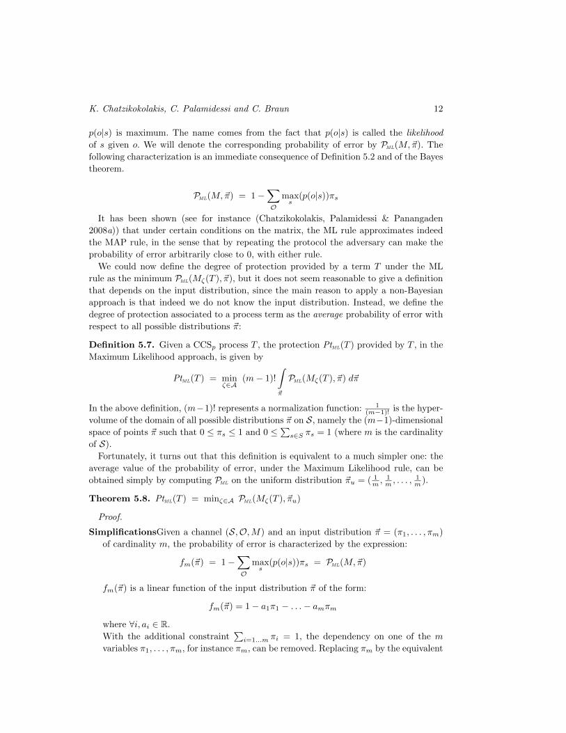
p(o|s) is maximum. The name comes from the fact that p(o|s) is called the likelihood

of s given o. We will denote the corresponding probability of error by PML(M,~π). The

following characterization is an immediate consequence of Definition 5.2 and of the Bayes

theorem.

PML(M,~π) = 1−∑O

maxs

(p(o|s))πs

It has been shown (see for instance (Chatzikokolakis, Palamidessi & Panangaden

2008a)) that under certain conditions on the matrix, the ML rule approximates indeed

the MAP rule, in the sense that by repeating the protocol the adversary can make the

probability of error arbitrarily close to 0, with either rule.

We could now define the degree of protection provided by a term T under the ML

rule as the minimum PML(Mζ(T ), ~π), but it does not seem reasonable to give a definition

that depends on the input distribution, since the main reason to apply a non-Bayesian

approach is that indeed we do not know the input distribution. Instead, we define the

degree of protection associated to a process term as the average probability of error with

respect to all possible distributions ~π:

Definition 5.7. Given a CCSp process T , the protection PtML(T ) provided by T , in the

Maximum Likelihood approach, is given by

PtML(T ) = minζ∈A

(m− 1)!

∫~π

PML(Mζ(T ), ~π) d~π

In the above definition, (m−1)! represents a normalization function: 1(m−1)! is the hyper-

volume of the domain of all possible distributions ~π on S, namely the (m−1)-dimensional

space of points ~π such that 0 ≤ πs ≤ 1 and 0 ≤∑s∈S πs = 1 (where m is the cardinality

of S).

Fortunately, it turns out that this definition is equivalent to a much simpler one: the

average value of the probability of error, under the Maximum Likelihood rule, can be

obtained simply by computing PML on the uniform distribution ~πu = ( 1m ,

1m , . . . ,

1m ).

Theorem 5.8. PtML(T ) = minζ∈A PML(Mζ(T ), ~πu)

Proof.

SimplificationsGiven a channel (S,O,M) and an input distribution ~π = (π1, . . . , πm)

of cardinality m, the probability of error is characterized by the expression:

fm(~π) = 1−∑O

maxs

(p(o|s))πs = PML(M,~π)

fm(~π) is a linear function of the input distribution ~π of the form:

fm(~π) = 1− a1π1 − . . .− amπm

where ∀i, ai ∈ R.

With the additional constraint∑i=1...m πi = 1, the dependency on one of the m

variables π1, . . . , πm, for instance πm, can be removed. Replacing πm by the equivalent


expression 1−∑m−1i=1 πi yields:

fm(~π) = c1π1 + . . .+ cm−1πm−1 + cm

with

c1 = am − a1

c2 = am − a2

. . .

cm−1 = am − am−1

cm = 1− amExpression of the normalization functionThe hyper-volume Vm(X) of the domain

Dm(X) of all possible distributions ~π on S, i.e. the (m − 1)-dimensional space of

points ~π such that 0 ≤ πs ≤ X and 0 ≤∑s∈S πs = X (where m is the cardinality of

S) is given by:

Vm(X) =Xm−1

(m− 1)!

Induction hypothesisWe will show by induction on m that following equalityHm holds

for all m: ∫Dm(X)

fm(~π)d~π = Vm(X)fm(~πu(X))

where ~πu(X) = (Xm ,Xm , . . . ,

Xm ). Theorem 5.8 then follows by taking X = 1.

According to the aforementioned notations, Hm can be written as:

Lm(X) = Rm(X)

where

Lm(X) =

X∫xm−1=0

X−xm−1∫xm−2=0

. . .

X−xm−1−...−x2∫x1=0

fm(x1, x2, . . . , xm−1)dx1dx2 . . . dxm−1

and

Rm(X) =Xm−1

(m− 1)!(

m−1∑i=1

ciX

m+ cm)

Base step: m = 2We have:

L2(X) =∫ x1=X

x1=0(c1x1 + c2)dx1

= c1X2

2 + c2X

= X( c1X2 + c2)

= R2(X)


Induction step: Hm ⇒ Hm+1Consider

fm+1(x) = c1x1 + . . .+ cmxm + cm+1

=∑mi=1 cixi + cm+1

= fm(x)− cm + cmxm + cm+1

The left-hand side of Hm+1 is given by:

Lm+1(X) =∫ xm=Y

xm=0. . .

∫ x1=Y−xm−...−x2

x1=0fm+1(x1, . . . , xm)dx1 . . . dxm

The m−1 inner-most integrations can be resolved according to Hm. Replacing X

by Y − xm leads to:

Lm+1(X) =∫ xm=Y

xm=0Vm(Y − xm)fm+1(Y−xm

m , . . . , Y−xm

m )dxm

=∫ xm=Y

xm=0(Y−xm)m−1

(m−1)! (∑m−1i=1 ci

Y−xm

m + cmxm + cm+1)dxm

Replacing Y − xm by Z leads to:

Lm+1(X) =∫ Z=Y

Z=0Zm−1

(m−1)! (∑m−1i=1 ci

Zm + cm(Y − Z) + cm+1)dZ

=∫ Z=Y

Z=0(( 1m!

∑m−1i=1 ci − cm

(m−1)! )Zm + cmY+cm+1

(m−1)! Zm−1)dZ

= ( 1(m+1)!

∑m−1i=1 ci)Y

m+1 − cm(m−1)!(m+1)Y

m+1 + cmm!Y

m+1 + cm+1

m! Ym

= ( 1(m+1)!

∑m−1i=1 ci)Y

m+1 + cm(m+1)!Y

m+1 + cm+1

m! Ym

= Ym

m! (∑mi=1 ci

Ym+1 + cm+1) = Rm+1(Y )

This completes the proof for Theorem 5.8.

The next corollary follows immediately from Theorem 5.8 and from the definitions of

PMAP and PML.

Corollary 5.9. PtML(T ) = minζ∈A PMAP(Mζ(T ), ~πu)

We conclude this section with some properties of PMAP . Note that the same properties

hold also for PML on the uniform distribution, because PML(M,~πu) = PMAP(M,~πu).

The next proposition shows that the probabilities of error are concave functions with

respect to the space of matrices.

Proposition 5.10. Consider a family of channels (S,O,Mi)i∈I , and a family cii∈Iof convex coefficients, namely 0 ≤ ci ≤ 1 for all i ∈ I, and

∑i∈I ci = 1. Then:

PMAP(∑i∈I

ciMi, ~π) ≥∑i∈I

ci PMAP(Mi, ~π)


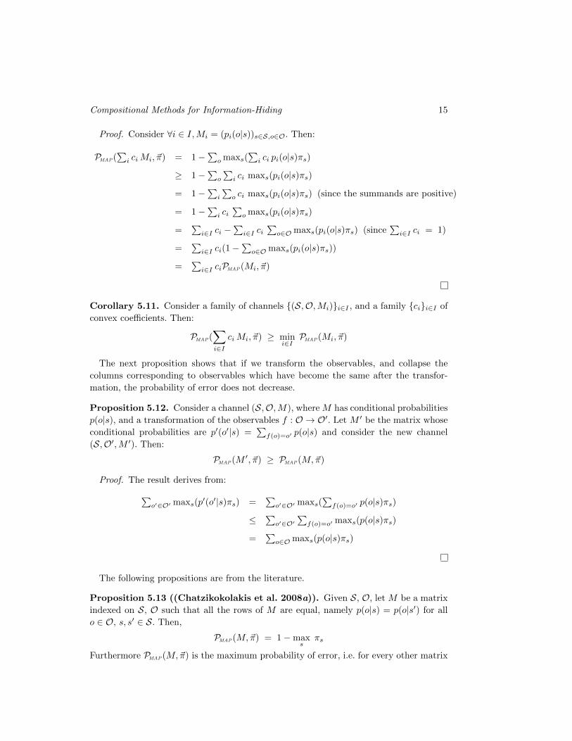
Proof. Consider ∀i ∈ I,Mi = (pi(o|s))s∈S,o∈O. Then:

PMAP(∑i ciMi, ~π) = 1−

∑o maxs(

∑i ci pi(o|s)πs)

≥ 1−∑o

∑i ci maxs(pi(o|s)πs)

= 1−∑i

∑o ci maxs(pi(o|s)πs) (since the summands are positive)

= 1−∑i ci

∑o maxs(pi(o|s)πs)

=∑i∈I ci −

∑i∈I ci

∑o∈Omaxs(pi(o|s)πs) (since

∑i∈I ci = 1)

=∑i∈I ci(1−

∑o∈Omaxs(pi(o|s)πs))

=∑i∈I ciPMAP(Mi, ~π)

Corollary 5.11. Consider a family of channels (S,O,Mi)i∈I , and a family cii∈I of

convex coefficients. Then:

PMAP(∑i∈I

ciMi, ~π) ≥ mini∈IPMAP(Mi, ~π)

The next proposition shows that if we transform the observables, and collapse the

columns corresponding to observables which have become the same after the transfor-

mation, the probability of error does not decrease.

Proposition 5.12. Consider a channel (S,O,M), where M has conditional probabilities

p(o|s), and a transformation of the observables f : O → O′. Let M ′ be the matrix whose

conditional probabilities are p′(o′|s) =∑f(o)=o′ p(o|s) and consider the new channel

(S,O′,M ′). Then:

PMAP(M ′, ~π) ≥ PMAP(M,~π)

Proof. The result derives from:∑o′∈O′ maxs(p

′(o′|s)πs) =∑o′∈O′ maxs(

∑f(o)=o′ p(o|s)πs)

≤∑o′∈O′

∑f(o)=o′ maxs(p(o|s)πs)

=∑o∈Omaxs(p(o|s)πs)

The following propositions are from the literature.

Proposition 5.13 ((Chatzikokolakis et al. 2008a)). Given S, O, let M be a matrix

indexed on S, O such that all the rows of M are equal, namely p(o|s) = p(o|s′) for all

o ∈ O, s, s′ ∈ S. Then,

PMAP(M,~π) = 1−maxs

πs

Furthermore PMAP(M,~π) is the maximum probability of error, i.e. for every other matrix


M ′ indexed on S, O we have:

PMAP(M,~π) ≥ PMAP(M ′, ~π)

Proposition 5.14 ((Bhargava & Palamidessi 2005)). Given a channel (S,O,M),

the rows of M are equal (and hence the probability of error is maximum) if and only if

p(s|o) = πs for all s ∈ S, o ∈ O.

The condition p(s|o) = πs means that the observation does not give any additional

information concerning the hypothesis. In other words, the a posteriori probability of s

coincides with its a priori probability. The property p(s|o) = πs for all s ∈ S and o ∈ Owas used as a definition of (strong) anonymity by Chaum (Chaum 1988) and was called

conditional anonymity by Halpern and O’Neill (Halpern & O’Neill 2005).

6. Safe constructs

In this section we investigate constructs of the language CCSp which are safe with respect

to the protection of the secrets.

We start by giving some conditions that will allow us to ensure the safety of the parallel

and the restriction operators.

Definition 6.1. Consider process term T , and the observables o1, o2, . . . , ok such that

(i) T does not contain any secret action, and

(ii) the observable actions of T are included in o1, o2, . . . , ok.

Then we say that T is safe outside of o1, o2, . . . , ok.

The following theorem states our main results for PtMAP . Note that they are also valid

for PtML, because PtML(T ) = PtMAP(T, ~πu).

Theorem 6.2. The probabilistic choice, the nondeterministic choice, and a restricted

form of parallel composition are safe constructs, namely, for every input probability π,

and any terms T1, T2, . . . , Th, we have

(1) PtMAP( ∑i

pi Ti, ~π) ≥∑i

pi PtMAP(Ti, ~π) ≥ mini

PtMAP(Ti, ~π)

(2) PtMAP(i

oi.Ti, ~π) = mini

PtMAP(Ti, ~π)

(3) PtMAP((ν o1, o2, . . . , ok) (T1 | T2)) ≥ PtMAP(T2, ~π)

if T1 is safe outside of o1, o2, . . . , ok.

Proof.

1 By definition PtMAP( ∑i pi Ti, ~π) = minζ∈A PMAP(Mζ(

∑i pi Ti), ~π).

Let ζm = minargA PMAP(Mζ( ∑i pi Ti), ~π). Hence

PtMAP( ∑i

pi Ti, ~π) = PMAP(Mζm( ∑i

pi Ti), ~π)

Consider, for each i, the scheduler ζmi defined as ζm on the i-th branch, except for


the removal of the first state and the first τ -step from the execution fragments in the

domain. It’s easy to see that

Mζm( ∑i

pi Ti) =∑i

piMζmi(Ti)

From Proposition 5.10 we derive

PMAP(Mζm( ∑i

pi Ti), ~π) ≥∑i

piPMAP(Mζmi(Ti), ~π)

Finally, observe that ζmiis still compatible with S, hence we have

PMAP(Mζmi(Ti), ~π) ≥ PtMAP(Ti, ~π) for all i

which concludes the proof in this case.

2 Let ζm = minargA PMAP(Mζ(i oi.Ti), ~π). LetAi be the class of schedulers that choose

the i-th branch at the beginning of the execution, and define

ζni = minargAi

PMAP(Mζ(i

oi.Ti), ~π)

Obviously we have

PtMAP(i

oi.Ti, ~π) = miniPMAP(Mζni

(i

oi.Ti), ~π)

Consider now, for each i, the scheduler ζmidefined as as ζni

, except for the removal

of the first state and the first step from the execution fragments in the domain.

Obviously ζmiis still compatible with S, and the observables of Ti are i one-to one

correspondence with those ofi oi.Ti via the bijective function fi(oioj1 . . . ojk) =

oj1 . . . ojk . Furthermore, all the probabilities of the channel Mζni(i oi.Ti) are the

same as those of Mζmi(Ti) modulo the renaming of o into f(o). Hence we have

PMAP(Mζni(i

oi.Ti), ~π) = PMAP(Mζmi(Ti), ~π) = PtMAP(Ti, ~π)

which concludes the proof of this case.

3 Let ζm = minargA PMAP(Mζ((νo1, o2, . . . , ok) (T1 | T2)), ~π). Hence

PtMAP((νo1, o2, . . . , ok) (T1 | T2), ~π) = PMAP(Mζm((νo1, o2, . . . , ok) (T1 | T2)), ~π)

The proof proceeds by constructing a set of series of schedulers whose limit with

respect to the metric d in Definition 5.3 correspond to schedulers on the execution

tree of T2. Consider a generic node in the execution tree of (νo1, o2, . . . , ok) (T1 | T2)

under ζm, and let (νo1, o2, . . . , ok) (T ′1 | T ′2) be the new term in that node. Assume

α to be the execution history up to that node. Let us consider separately the three

possible kinds of transitions derivable from the operational semantics:

(a) (νo1, o2, . . . , ok) (T ′1 | T ′2)a−→ (νo1, o2, . . . , ok) (µ | T ′2) due to a transition T ′1

a−→µ. In this case a must be τ because of the assumption that T1 does not contain

secret actions and all its observable actions are included in o1, o2, . . . , ok. Assume

that µ =∑i pi δ(T

′1i). Then we have (νo1, o2, . . . , ok) (µ | T ′2) =

∑i pi δ((νo1, o2, . . . , ok) (T ′1i | T ′2)).

Let us consider the tree obtained by replacing this distribution with δ((νo1, o2, . . . , ok) (T ′1i | T ′2))


(i.e. the tree obtained by pruning all alternatives except (νo1, o2, . . . , ok) (T ′1i | T ′2),

and assigning to it probability 1). Let ζmi be the projection of ζm on the new tree

(i.e. ζmi is defined as the projection of ζm on the histories α′ such that if α is a

proper prefix of α′ then ατ(νo1, o2, . . . , ok) (T ′1i | T ′2) is a prefix of α′). We have

PMAP(Mζm((νo1, o2, . . . , ok) (T1 | T2)), ~π)

=

PMAP(∑i pi Mζmi

((νo1, o2, . . . , ok) (T1 | T2)), ~π)

≥ (by Proposition 5.10)∑i pi PMAP(Mζmi

((νo1, o2, . . . , ok) (T1 | T2)), ~π)

In the execution tree of T2 the above transition does not have a correspondent, but

it obliges us to consider all different schedulers that are associated to the various

ζmi’s for different i’s.

(b) (νo1, o2, . . . , ok) (T ′1 | T ′2)a−→ (νo1, o2, . . . , ok) (T ′1 | µ) due to a transition T ′2

a−→µ, with a not included in o1, o2, . . . , ok. In this case, the corresponding scheduler

for T2 must choose the same transition, i.e. T ′2a−→ µ.

(c) (νo1, o2, . . . , ok) (T ′1 | T ′2)τ−→ (νo1, o2, . . . , ok) δ(T ′′1 | T ′′2 ) due to the transitions

T ′1a−→ δ(T ′′1 ) and T ′2

a−→ δ(T ′′2 ). In this case a must be an observable o because

of the assumption that T1 does not contain secret actions. The corresponding

scheduler for T2 must choose the transition T ′2a−→ δ(T ′′2 ).

By considering the inequalities given by the transitions of type (a), we obtain


≥∑i pi PMAP(Mζmi((νo1, o2, . . . , ok) (T1 | T2)), ~π)

≥∑i pi

∑j qj PMAP(Mζmij

((νo1, o2, . . . , ok) (T1 | T2)), ~π)

≥∑i pi

∑j qj

∑h rh PMAP(Mζmijh

((νo1, o2, . . . , ok) (T1 | T2)), ~π)

≥

. . .

Observe now that ζm, ζmi, ζmij , ζmijh, . . . is a converging series of schedulers whose

limit ζmijh... is isomorphic to a scheduler for T2, except that some of the observable

transitions in T2 may be removed due to the restriction on o1, o2, . . . , ok. This removal


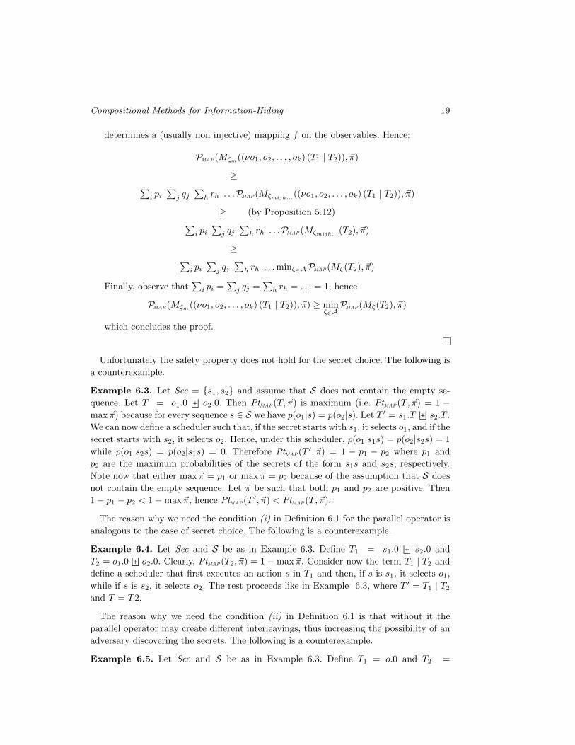
determines a (usually non injective) mapping f on the observables. Hence:


≥∑i pi

∑j qj

∑h rh . . .PMAP(Mζmijh...

((νo1, o2, . . . , ok) (T1 | T2)), ~π)

≥ (by Proposition 5.12)∑i pi

∑j qj

∑h rh . . .PMAP(Mζmijh...

(T2), ~π)

≥∑i pi

∑j qj

∑h rh . . .minζ∈A PMAP(Mζ(T2), ~π)

Finally, observe that∑i pi =

∑j qj =

∑h rh = . . . = 1, hence

PMAP(Mζm((νo1, o2, . . . , ok) (T1 | T2)), ~π) ≥ minζ∈APMAP(Mζ(T2), ~π)


Unfortunately the safety property does not hold for the secret choice. The following is

a counterexample.

Example 6.3. Let Sec = s1, s2 and assume that S does not contain the empty se-

quence. Let T = o1.0o2.0. Then PtMAP(T, ~π) is maximum (i.e. PtMAP(T, ~π) = 1 −

max~π) because for every sequence s ∈ S we have p(o1|s) = p(o2|s). Let T ′ = s1.Ts2.T .

We can now define a scheduler such that, if the secret starts with s1, it selects o1, and if the

secret starts with s2, it selects o2. Hence, under this scheduler, p(o1|s1s) = p(o2|s2s) = 1

while p(o1|s2s) = p(o2|s1s) = 0. Therefore PtMAP(T ′, ~π) = 1 − p1 − p2 where p1 and

p2 are the maximum probabilities of the secrets of the form s1s and s2s, respectively.

Note now that either max~π = p1 or max~π = p2 because of the assumption that S does

not contain the empty sequence. Let ~π be such that both p1 and p2 are positive. Then

1− p1 − p2 < 1−max~π, hence PtMAP(T ′, ~π) < PtMAP(T, ~π).

The reason why we need the condition (i) in Definition 6.1 for the parallel operator is

analogous to the case of secret choice. The following is a counterexample.

Example 6.4. Let Sec and S be as in Example 6.3. Define T1 = s1.0s2.0 and

T2 = o1.0o2.0. Clearly, PtMAP(T2, ~π) = 1−max~π. Consider now the term T1 | T2 and

define a scheduler that first executes an action s in T1 and then, if s is s1, it selects o1,

while if s is s2, it selects o2. The rest proceeds like in Example 6.3, where T ′ = T1 | T2

and T = T2.

The reason why we need the condition (ii) in Definition 6.1 is that without it the

parallel operator may create different interleavings, thus increasing the possibility of an

adversary discovering the secrets. The following is a counterexample.

Example 6.5. Let Sec and S be as in Example 6.3. Define T1 = o.0 and T2 =


s1.(o1.0 ⊕.5 o2.0)s2.(o1.0 ⊕.5 o2.0). It is easy to see that PtMAP(T2, ~π) = 1−max~π.

Consider the term T1 | T2 and define a scheduler that first executes an action s in

T2 and then, if s is s1, it selects first T1 and then the continuation of T2, while if s

is s2, it selects first the continuation of T2 and then T1. Hence, under this scheduler,

p(oo1|s1s) = p(oo2|s1s) = .5 and also p(o1o|s2s) = p(o2o|s2s) = .5 while p(oo1|s2s) =

p(oo2|s2s) = 0 and p(o1o|s1s) = p(o2o|s1s) = 0. Therefore PtMAP(T, ~π) = 1 − p1 − p2

where p1 and p2 are the maximum probabilities of the secrets of the form s1s and s2s,

respectively. Following the same reasoning as in Example 6.3, we have that for certain

~π, PtMAP(T ′, ~π) < PtMAP(T, ~π).

7. A case study: the Dining Cryptographers

In this section we consider the Dining Cryptographers (DC) protocol proposed by Chaum

(Chaum 1988), we show how to describe it in CCSp, and we apply the results of previous

section to obtain a generalization of Chaum’s strong anonymity result.

In its most general formulation, the DC consists of a multigraph where one of the nodes

(cryptographers) may be secretly designated to pay for the dinner. The cryptographers

would like to find out whether there is a payer or not, but without either discovering the

identity of the payer, nor revealing it to an external observer. The problem can be solved

as follows: we put on each edge a probabilistic coin, which can give either 0 or 1. The

coins get tossed, and each cryptographer computes the binary sum of all (the results of)

the adjacent coins. Furthermore, it adds 1 if it is designated to be the payer. Finally, all

the cryptographers declare their result.

It is easy to see that this protocol solves the problem of figuring out the existence of a

payer: the binary sum of all declarations is 1 if and only if there is a payer, because all

the coins get counted twice, so their contribution to the total sum is 0.

The property we are interested in, however, is the anonymity of the system. Chaum

proved that the DC is strongly anonymous if all the coins are fair, i.e. they give 0 and 1

with equal probability, and the multigraph is connected, namely there is a path between

each pair of nodes. To state formally the property, let us denote by s the secret identity

of the payer, and by o the collection of the declarations of the cryptographers.

Theorem 7.1 ((Chaum 1988)). If the multigraph is connected, and the coins are fair,

then DC is strongly anonymous, namely for every s and o, p(s|o) = p(s) holds.

We are now going to show how to express the DC in CCSp. We start by introducing a

notation for value-passing in CCSp, following standard lines.

Input c(x).T =v

cv.T [v/x]

Output c〈v〉 = cv

The protocol can be described as the parallel composition of the cryptographers pro-

cesses Crypt i, of the coin processes Coinh, and of a process Collect whose purpose is to

collect all the declarations of the cryptographers, and output them in the form of a tuple.


Crypti = ci,i1 (x1) . . . . . ci,ik (xk) . payi(x) . di〈x1 + . . .+ xk + x〉

Coinh = c`,h〈0〉 . cr,h〈0〉.0 ⊕ph c`,h〈1〉 . cr,h〈1〉.0

Collect = d1(y1) . d2(y2) . . . . . dn(yn) . out〈y1, y2, . . . , yn〉

DC = (ν~c)(ν ~d)(∏i Crypti |

∏h Coinh | Collect)

Table 2. The dining cryptographers protocol expressed in CCSp.

See Table 2. In this protocol, the secret actions are pay i. All the others are observable

actions.

Each coin communicates with two cryptographers. ci,h represents the communication

channel between Coinh and Crypt i if h is indeed the index of a coin, otherwise it repre-

sents a communication channel “with the environment”. We will call the latter external.

In the original definition of the DC there are no external channels, we have added them

to prove a generalization of Chaum’s result. They could be interpreted as a way for

the environment to influence the computation of the cryptographers and hence test the

system, for the purpose of discovering the secret.

We are now ready to state our generalization of Chaum’s result:

Theorem 7.2. A DC is strongly anonymous if it has a spanning tree consisting of fair

coins only.

Proof. Consider the term DC in Table 2. Remove all the coins that do not belong to

the spanning tree, and the corresponding restriction operators. Let T be the process term

obtained this way. Let A be the class of schedulers which select the value 0 for all the

external channels. This situation corresponds to the original formulation of Chaum and

so we can apply Chaum’s result (Theorem 7.1) and Proposition 5.14 to conclude that all

the rows of the matrix M are the same and hence, by Proposition 5.13, PMAP(M,~π) =

1−maxi πi.

Consider now one of the removed coins, h, and assume, without loss of generality, that

c`,h(x), cr,h(x) are the first actions in the definitions of Crypt` and Cryptr. Consider

the class of schedulers B that selects value 1 for x in these channels. The matrix M ′

that we obtain is isomorphic to M : the only difference is that each column o is now

mapped to a column o + w, where w is a tuple that has 1 in the ` and r positions,

and 0 in all other positions, and + represents the componentwise binary sum. Since this

map is a bijection, we can apply Proposition 5.12 in both directions and derive that

PMAP(M ′, ~π) = 1−maxi πi.

By repeating the same reasoning on each of the removed coins, we can conclude that

PtMAP(T, ~π) = 1−maxi πi for any scheduler ζ of T .

Consider now the term T ′ obtained from T by adding back the coin h:

T ′ = (νc`,hcr,h)(Coinh | T )


By applying Theorem 6.2 we can deduce that

PtMAP(T ′, ~π) ≥ PtMAP(T, ~π)

By repeating this reasoning, we can add back all the coins, one by one, and obtain the

original DC . Hence we can conclude that

PtMAP(DC , ~π) ≥ PtMAP(T, ~π) = 1−maxiπi

and, since 1−maxi πi is the maximum probability of error,

PtMAP(DC , ~π) = 1−maxiπi


Interestingly, also the other direction of Theorem 7.2 holds. We report this result for

completeness, however we have proved it by using traditional methods, not by applying

the compositional methods of Section 6.

Theorem 7.3. A DC is strongly anonymous only if it has a spanning tree consisting of

fair coins only.

Proof. By contradiction. Let G be the multigraph associated to the DC and let n be

the number of vertices in G. Assume that G does not have a spanning tree consisting

only of fair coins. Then it is possible to split G in two non-empty subgraphs, G1 and G2,

such that all the edges between G1 and G2 are unfair. Let (c1, c2, . . . , cm) be the vector

of coins corresponding to these edges. Since G is connected, we have that m ≥ 1.

Let a1 be a vertex in G1 and a2 be a vertex in G2. By strong anonymity, for every

observable o we have

p(o | a1) = p(o | a2) (1)

Where a1, resp. a2, represents the event that the chryptographer a1, resp. a2, is the

payer.

Observe now that p(o | a1) = p(o + w | a2) where w is a binary vector of dimension

n containing 1 exactly twice, in correspondence of a1 and a2, and + is the binary sum.

Hence (1) becomes

p(o+ w | a2) = p(o | a2) (2)

Let d be the binary sum of all the elements of o in G1, and d′ be the binary sum of all

the elements of o+ w in G1. Since in G1 w contains 1 exactly once, we have d′ = d+ 1.

Hence (2), being valid for all o’s, implies

p(d+ 1 | a2) = p(d | a2) (3)

Because of the way o, and hence d, are calculated, and since the contribution of the edges

internal to G1 is 0, and a2 (the payer) is not in G1, we have that

d =

m∑i=1

ci


from which, together with (3), and the fact that the coins are independent from the

choice of the payer, we derive

p(

m∑i=1

ci = 0) = p(

m∑i=1

ci = 1) = 1/2 (4)

The last step is to prove that p(∑mi=1 ci = 0) = 1/2 implies that one of the ci’s is

fair, which will give us a contradiction. We prove this by induction on m. The prop-

erty obviously holds for m = 1. Let us now assume that we have proved it for the

vector (c1, c2, . . . , cm−1). Observe that p(∑mi=1 ci = 0) = p(

∑m−1i=1 ci = 0)p(cm = 0) +

p(∑m−1i=1 ci = 1)p(cm = 1). From (4) we derive

p(

m−1∑i=1

ci = 0)p(cm = 0) + p(

m−1∑i=1

ci = 1)p(cm = 1) = 1/2 (5)

Now, it is easy to see that (5) has only two solutions: one in which p(cm = 0) = 1/2, and

one in which p(∑m−1i=1 ci = 1) = 1/2. In the first case we are done, in the second case we

apply the induction hypothesis.

8. Related work

In the field of information flow there have been various works (McLean 1990, Gray,

III 1991, Lowe 2002, Clark, Hunt & Malacaria 2001, Clark, Hunt & Malacaria 2005,

Malacaria 2007, Malacaria & Chen 2008, Heusser & Malacaria 2009, Smith 2009, Andres,

Palamidessi, van Rossum & Smith 2010, Alvim, Andres & Palamidessi 2010, Boreale,

Pampaloni & Paolini 2011) in which the high information and the low information are

seen as the input and output respectively of a (noisy) channel. Information leakage is

formalized in this setting as the channel mutual information or the channel capacity. The

idea is that the leakage represents the difference between the a priori uncertainty about

the (secret) high information, and the a posteriori uncertainty, after the low information

has become pubblically known. The uncertainty is expressed in terms of entropy, and

there are various alternative notions depending on the notion of attack that one wishes

to model, as discussed in (Kopf & Basin 2007). Most of the above approaches are based

either on Shannon entropy or on the Renyi min entropy.

Channel capacity has been also used in relation to anonymity in (Moskowitz, Newman,

Crepeau & Miller 2003b, Moskowitz, Newman & Syverson 2003a). These works propose

a method to create covert communication by means of non-perfect anonymity.

A related line of work is (Serjantov & Danezis 2002, Dıaz, Seys, Claessens & Preneel

2002), where the main idea is to express the lack of (probabilistic) information in terms

of entropy.

A different information-theoretic approach is taken in (Clarkson, Myers & Schneider

2009). In this paper, the authors define as information leakage the difference between

the a priori accuracy of the guess of the attacker, and the a posteriori one, after the

attacker has made his observation. The accuracy of the guess is defined as the Kullback-

Leibler distance between the belief (which is a weight attributed by the attacker to each


input hypothesis) and the true distribution on the hypotheses. This approach, that was

Shannon-based in (Clarkson et al. 2009), was later applied by Hamadou et al. (Hamadou,

Palamidessi & Sassone 2010) also to the case of the Renyi min entropy.

The problem of preservation of information protection under program composition was

considered also by McIver et al (McIver et al. 2010). In that paper, the author define

an order on specifications based on Bayes Risk, and they identify a compositional

subset of it: a refinement order v such that S v I implies C[S] C[I] for all contexts

C. They also show that v is the compositional closure of , in the sense that S 6v I

only when C[S] 6 C[I] for some C. Finally, they prove that v is sound for other three,

competing notions of elementary test and that therefore Bayes-Risk testing, with context,

is maximally discriminating among them.

Desharnais et al. (Desharnais, Jagadeesan, Gupta & Panangaden 2002) defined a no-

tion of metric between probabilistic processes and proved that the Shannon capacity

associated to a protocol associated to a process is continuous with respect to this metric.

Deng et al. (Deng, Pang & Wu 2006) consider a probabilistic calculus similar to CCSp,

and define a relation between traces based on the Kullback-Leibler divergence. They show

that certain constructs of their calculus preserve the relation, in the sense that they do

not increase the divergence.

9. Conclusion and future work

In this paper we have investigated the properties of the probability of error associated

to a given information-hiding protocol, and we have investigated CCSpconstructs that

are safe, i.e. that are guaranteed not to decrease the protection of the protocol. Then we

have applied these results to strengthen a result of Chaum: the dining cryptographers

are strongly anonymous if and only if they have a spanning tree of fair coins.

In the future, we would like to extend our results to other constructs of the language.

This is not possible in the present setting, as the examples after Theorem 6.2 show. The

problem is related to the scheduler: the standard notion of scheduler is too powerful and

can leak secrets, by depending on the secret choices that have been made in the past. All

the examples after Theorem 6.2 are based on this kind of problem. In (Chatzikokolakis &

Palamidessi 2010), we have studied the problem and we came out with a language-based

solution to restrict the power of the scheduler. We are planning to investigate whether

such approach could be exploited here to guarantee the safety of more constructs.

References

Alvim, M. S., Andres, M. E. & Palamidessi, C. (2010), Information Flow in Interactive Systems,

in P. Gastin & F. Laroussinie, eds, ‘Proceedings of the 21th International Conference on

Concurrency Theory (CONCUR 2010), Paris, France, August 31-September 3’, Vol. 6269 of

Lecture Notes in Computer Science, Springer, pp. 102–116.

Andres, M. E., Palamidessi, C., van Rossum, P. & Smith, G. (2010), Computing the leakage of

information-hiding systems, in J. Esparza & R. Majumdar, eds, ‘Proceedings of the 16th In-

ternational Conference on Tools and Algorithms for the Construction and Analysis of Systems

(TACAS 2010)’, Vol. 6015 of Lecture Notes in Computer Science, Springer, pp. 373–389.


Bhargava, M. & Palamidessi, C. (2005), Probabilistic anonymity, in M. Abadi & L. de Alfaro,

eds, ‘Proceedings of CONCUR’, Vol. 3653 of Lecture Notes in Computer Science, Springer,

pp. 171–185.

Boreale, M., Pampaloni, F. & Paolini, M. (2011), Asymptotic information leakage under one-

try attacks, in M. Hofmann, ed., ‘Proceedings of the 14th International Conference on the

Foundations of Software Science and Computational Structures (FOSSACS)’, Vol. 6604 of

Lecture Notes in Computer Science, Springer, pp. 396–410.

Chatzikokolakis, K. & Palamidessi, C. (2010), ‘Making random choices invisible to the scheduler’,

Information and Computation 208(6), 694–715.

Chatzikokolakis, K., Palamidessi, C. & Panangaden, P. (2008a), ‘Anonymity protocols as noisy

channels’, Inf. and Comp. 206(2–4), 378–401.

Chatzikokolakis, K., Palamidessi, C. & Panangaden, P. (2008b), ‘On the Bayes risk in

information-hiding protocols’, Journal of Computer Security 16(5), 531–571.

Chaum, D. (1988), ‘The dining cryptographers problem: Unconditional sender and recipient

untraceability’, Journal of Cryptology 1, 65–75.

Clark, D., Hunt, S. & Malacaria, P. (2001), Quantitative analysis of the leakage of confidential

data, in ‘Proceedings of the Workshop on Quantitative Aspects of Programming Languages’,

Vol. 59 (3) of Electr. Notes Theor. Comput. Sci, Elsevier Science B.V., pp. 238–251.

Clark, D., Hunt, S. & Malacaria, P. (2005), Quantified interference for a while language, in

‘Proceedings of the Second Workshop on Quantitative Aspects of Programming Languages

(QAPL 2004)’, Vol. 112 of Electronic Notes in Theoretical Computer Science, Elsevier Science

B.V., pp. 149–166.

Clarkson, M. R., Myers, A. C. & Schneider, F. B. (2009), ‘Belief in information flow’, Journal of

Computer Security 17(5), 655–701.

Cover, T. M. & Thomas, J. A. (1991), Elements of Information Theory, John Wiley & Sons, Inc.

Deng, Y., Palamidessi, C. & Pang, J. (2005), Compositional reasoning for probabilistic finite-

state behaviors, in A. Middeldorp, V. van Oostrom, F. van Raamsdonk & R. C. de Vrijer, eds,

‘Processes, Terms and Cycles: Steps on the Road to Infinity’, Vol. 3838 of Lecture Notes in

Computer Science, Springer, pp. 309–337. http://www.lix.polytechnique.fr/~catuscia/

papers/Yuxin/BookJW/par.pdf.

Deng, Y., Pang, J. & Wu, P. (2006), Measuring anonymity with relative entropy, in T. Dimitrakos,

F. Martinelli, P. Y. A. Ryan & S. A. Schneider, eds, ‘Proc. of the of the 4th Int. Worshop on

Formal Aspects in Security and Trust’, Vol. 4691 of LNCS, Springer, pp. 65–79.

Desharnais, J., Jagadeesan, R., Gupta, V. & Panangaden, P. (2002), The metric analogue of weak

bisimulation for probabilistic processes, in ‘Proceedings of the 17th Annual IEEE Symposium

on Logic in Computer Science’, IEEE Computer Society, pp. 413–422.

Dıaz, C., Seys, S., Claessens, J. & Preneel, B. (2002), Towards measuring anonymity, in R. Dingle-

dine & P. F. Syverson, eds, ‘Proceedings of the workshop on Privacy Enhancing Technologies

(PET) 2002’, Vol. 2482 of Lecture Notes in Computer Science, Springer, pp. 54–68.

Fujioka, A., Okamoto, T. & Ohta, K. (1993), A practical secret voting scheme for large scale

elections, in ‘ASIACRYPT ’92: Proceedings of the Workshop on the Theory and Application

of Cryptographic Techniques’, Springer-Verlag, London, UK, pp. 244–251.

Gray, III, J. W. (1991), Toward a mathematical foundation for information flow security, in

‘Proceedings of the 1991 IEEE Computer Society Symposium on Research in Security and

Privacy (SSP ’91)’, IEEE, Washington - Brussels - Tokyo, pp. 21–35.

Halpern, J. Y. & O’Neill, K. R. (2005), ‘Anonymity and information hiding in multiagent sys-

tems’, Journal of Computer Security 13(3), 483–512.


Hamadou, S., Palamidessi, C. & Sassone, V. (2010), Reconciling belief and vulnerability in in-

formation flow, in ‘Proceedings of the 31st IEEE Symposium on Security and Privacy’, IEEE

Computer Society, pp. 79–92.

Herescu, O. M. & Palamidessi, C. (2000), Probabilistic asynchronous π-calculus, in J. Tiuryn,

ed., ‘Proceedings of FOSSACS 2000 (Part of ETAPS 2000)’, Vol. 1784 of Lecture Notes in

Computer Science, Springer, pp. 146–160. http://www.lix.polytechnique.fr/~catuscia/

papers/Prob_asy_pi/fossacs.ps.

Heusser, J. & Malacaria, P. (2009), Applied quantitative information flow and statistical

databases, in P. Degano & J. D. Guttman, eds, ‘Proceedings of the International Workshop

on Formal Aspects in Security and Trust’, Vol. 5983 of Lecture Notes in Computer Science,

Springer, pp. 96–110.

Kopf, B. & Basin, D. A. (2007), An information-theoretic model for adaptive side-channel attacks,

in P. Ning, S. D. C. di Vimercati & P. F. Syverson, eds, ‘Proceedings of the 2007 ACM

Conference on Computer and Communications Security, CCS 2007, Alexandria, Virginia,

USA, October 28-31, 2007’, ACM, pp. 286–296.

Lowe, G. (2002), Quantifying information flow, in ‘Proc. of CSFW 2002’, IEEE Computer Society

Press, pp. 18–31.

Malacaria, P. (2007), Assessing security threats of looping constructs, in M. Hofmann &

M. Felleisen, eds, ‘Proceedings of the 34th ACM SIGPLAN-SIGACT Symposium on Prin-

ciples of Programming Languages, POPL 2007, Nice, France, January 17-19, 2007’, ACM,

pp. 225–235.

Malacaria, P. & Chen, H. (2008), Lagrange multipliers and maximum information leakage in

different observational models, in Ulfar Erlingsson and Marco Pistoia, ed., ‘Proceedings of

the 2008 Workshop on Programming Languages and Analysis for Security (PLAS 2008)’,

ACM, Tucson, AZ, USA, pp. 135–146.

McIver, A., Meinicke, L. & Morgan, C. (2010), Compositional closure for bayes risk in probabilis-

tic noninterference, in S. Abramsky, C. Gavoille, C. Kirchner, F. M. auf der Heide & P. G.

Spirakis, eds, ‘Proceedings of the 37th International Colloquium on Automata, Languages and

Programming (ICALP). Part II.’, Vol. 6199 of Lecture Notes in Computer Science, Springer,

pp. 223–235.

McLean, J. (1990), Security models and information flow, in ‘SSP’90’, IEEE, pp. 180–189.

Milner, R. (1989), Communication and Concurrency, International Series in Computer Science,

Prentice Hall.

Moskowitz, I. S., Newman, R. E. & Syverson, P. F. (2003a), Quasi-anonymous channels, in ‘Proc.

of CNIS’, IASTED, pp. 126–131.

Moskowitz, I. S., Newman, R. E., Crepeau, D. P. & Miller, A. R. (2003b), Covert channels

and anonymizing networks., in S. Jajodia, P. Samarati & P. F. Syverson, eds, ‘Workshop on

Privacy in the Electronic Society 2003’, ACM, pp. 79–88.

Palamidessi, C. & Herescu, O. M. (2005), ‘A randomized encoding of the π-calculus with mixed

choice’, Theoretical Computer Science 335(2-3), 373–404. http://www.lix.polytechnique.

fr/~catuscia/papers/prob_enc/report.pdf.

Reiter, M. K. & Rubin, A. D. (1998), ‘Crowds: anonymity for Web transactions’, ACM Trans-

actions on Information and System Security 1(1), 66–92.

Renyi, A. (1961), On Measures of Entropy and Information, in ‘Proceedings of the 4th Berkeley

Symposium on Mathematics, Statistics, and Probability’, pp. 547–561.

Segala, R. (1995), Modeling and Verification of Randomized Distributed Real-Time Systems,

PhD thesis. Tech. Rep. MIT/LCS/TR-676.


Segala, R. & Lynch, N. (1995), ‘Probabilistic simulations for probabilistic processes’, Nordic Jour-

nal of Computing 2(2), 250–273. An extended abstract appeared in Proceedings of CONCUR

’94, LNCS 836: 481-496.

Serjantov, A. & Danezis, G. (2002), Towards an information theoretic metric for anonymity.,

in R. Dingledine & P. F. Syverson, eds, ‘Proceedings of the workshop on Privacy Enhancing

Technologies (PET) 2002’, Vol. 2482 of Lecture Notes in Computer Science, Springer, pp. 41–

53.

Smith, G. (2009), On the foundations of quantitative information flow, in L. de Alfaro, ed., ‘Proc.

of the 12th Int. Conf. on Foundations of Software Science and Computation Structures’, Vol.

5504 of LNCS, Springer, York, UK, pp. 288–302.

compositional methods for information-hiding

Documents