computational challenges from imaging x-ray polarimetry

Computational Challenges from Imaging

X-ray PolarimetryHerman L. Marshall (MIT)

and the IXPE Team

Imaging Polarimetry CHASC 2/6/18

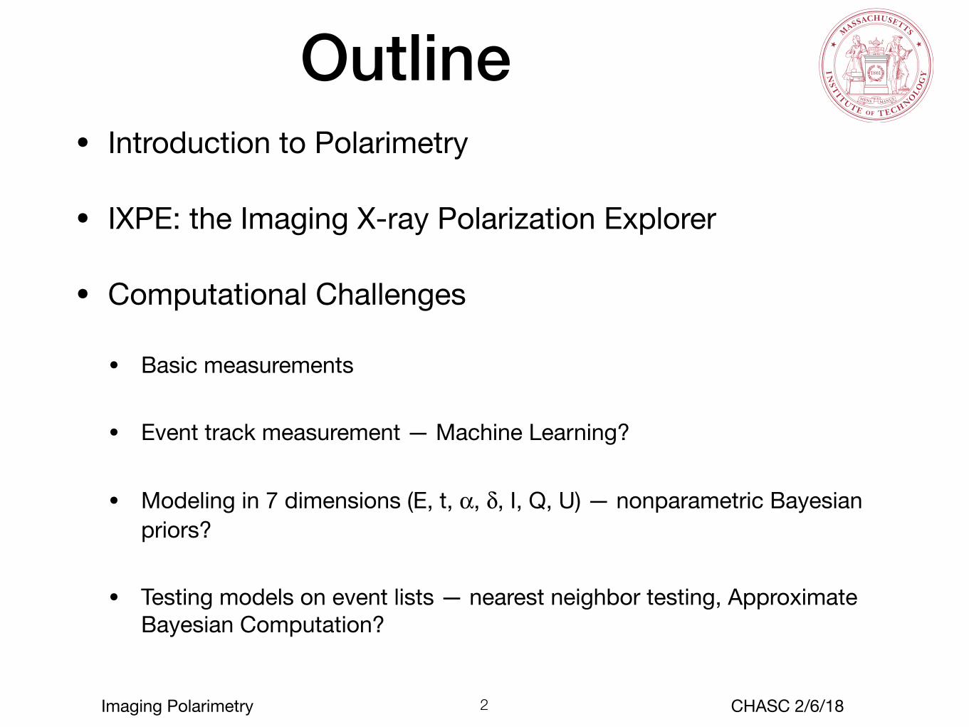
Outline• Introduction to Polarimetry

• IXPE: the Imaging X-ray Polarization Explorer

• Computational Challenges

• Basic measurements

• Event track measurement — Machine Learning?

• Modeling in 7 dimensions (E, t, a, d, I, Q, U) — nonparametric Bayesian priors?

• Testing models on event lists — nearest neighbor testing, Approximate Bayesian Computation?

2


Polarimetry Probes of Physics

3


Basics of Polarized Light• All light waves are polarized

• Stokes parameters are handy:• I = total intensity

• Q, U are orthogonal linearly polarized parts

• V is circular (+ or -) polarized intensity

• Common alternative: P, f

• P = (Q2 + U2)1/2 / I

• f = tan-1(Q/U)

• A beam is “unpolarized” if the photon set is randomly polarized (P = V = 0)

• MDP = ‘Minimum Detectable Polarization’ (99% conf.):

• All photons also have energy (E), time (t), sky position (a,d)

4


Modulation of Polarized Signals

5

Modulation Factor = µ = (Cmax-Cmin)/(Cmax+Cmin)

http://www.isdc.unige.ch/polar/modfactor

http://www.isdc.unige.ch/polar/modfactor


AGN Jet Polarimetry (M 87)

6

Marshall et al. 2002

Perlman+ ‘12


Testing Quantum Electrodynamics with Magnetars

• Magnetars: slowly rotating neutron stars with B > 1014 G

• Magnetized vacuum is birefringent

• Flux is unaffected but polarization fraction and angle change with spin phase

7


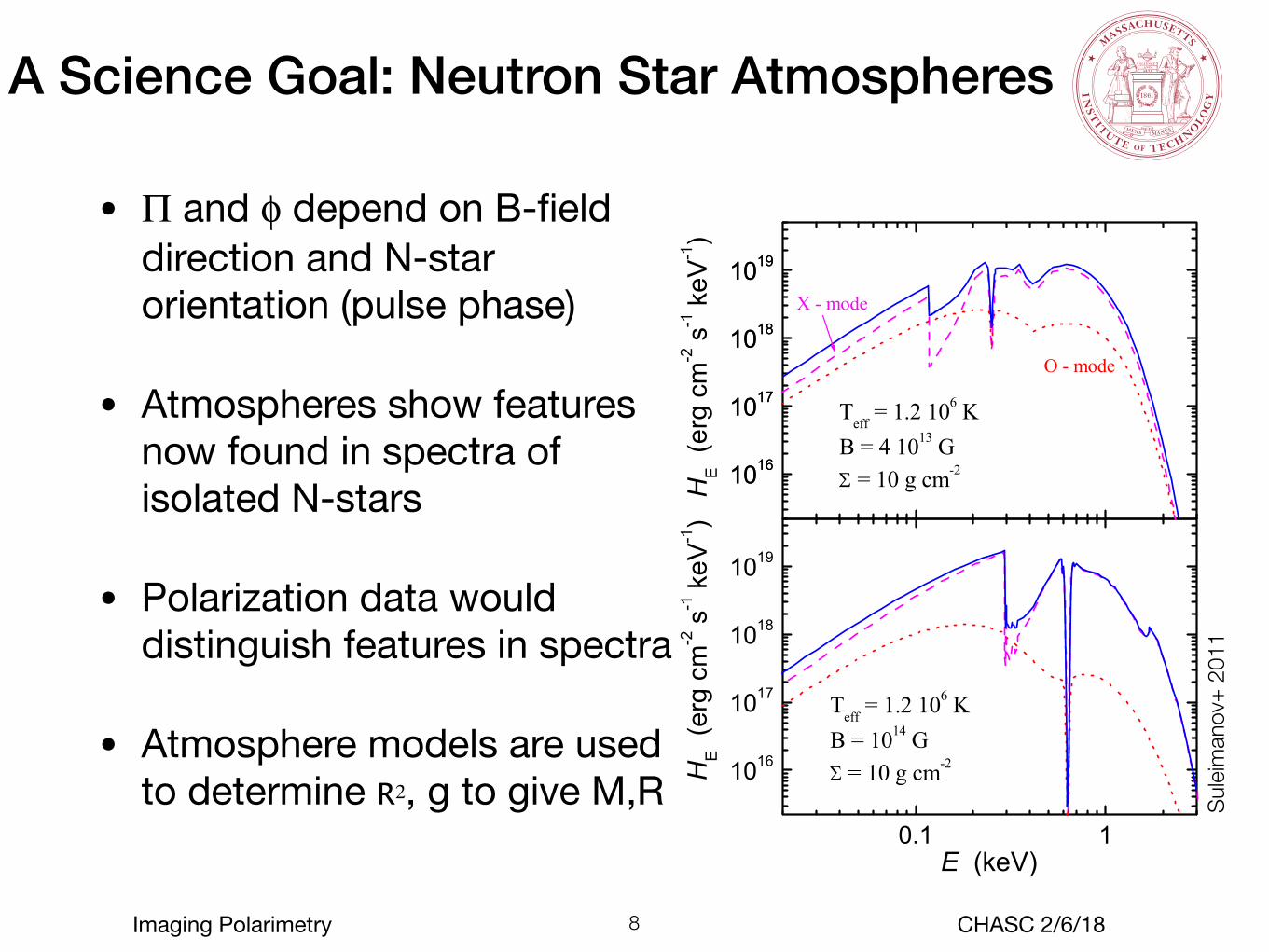
A Science Goal: Neutron Star Atmospheres

• P and f depend on B-field direction and N-star orientation (pulse phase)

• Atmospheres show features now found in spectra of isolated N-stars

• Polarization data would distinguish features in spectra

• Atmosphere models are used to determine R2, g to give M,R

8

0.1 1

1016

1017

1018

1019

1016

1017

1018

1019

1016

1017

1018

1019

HE

(erg

cm

-2 s

-1 k

eV-1)

X - mode

O - mode

Teff = 1.2 106 KB = 4 1013 G6 = 10 g cm-2

Teff = 1.2 106 KB = 1014 G6 = 10 g cm-2

E (keV)

HE

(erg

cm

-2 s

-1 k

eV-1)

Sulei

man

ov+

2011


Imaging X-ray Polarization Explorer (IXPE)

9

ForwardStarTracker

MirrorModuleAssembly(×3)

X-rayShields(×3)deployed

Boomw/ThermalSockdeployed

DetectorUnit(×3)

Spacecraftw/Avionics

SolarArray

5.2-mtotallengthdeployed

4.0-mfocallength


IXPE Gas Pixel Detector

10

StrayX-rayCollimatorFilterCalibration

Wheel(FCW)Hub

FilterCalibrationWheel(FCW)Motor

GasPixelDetector(GPD)Housing


Event Results• Event time (to 10 µs), image, pulses measured

• Empirical method finds event origin, direction

11


Polarization from modulation histogram and calibrated modulation factor

12

Actualdataforapolarizedsource

40.7%±0.3%modulation

Actualdataforanunpolarizedsource

0.6%±0.4%modulation

MDP.99 =


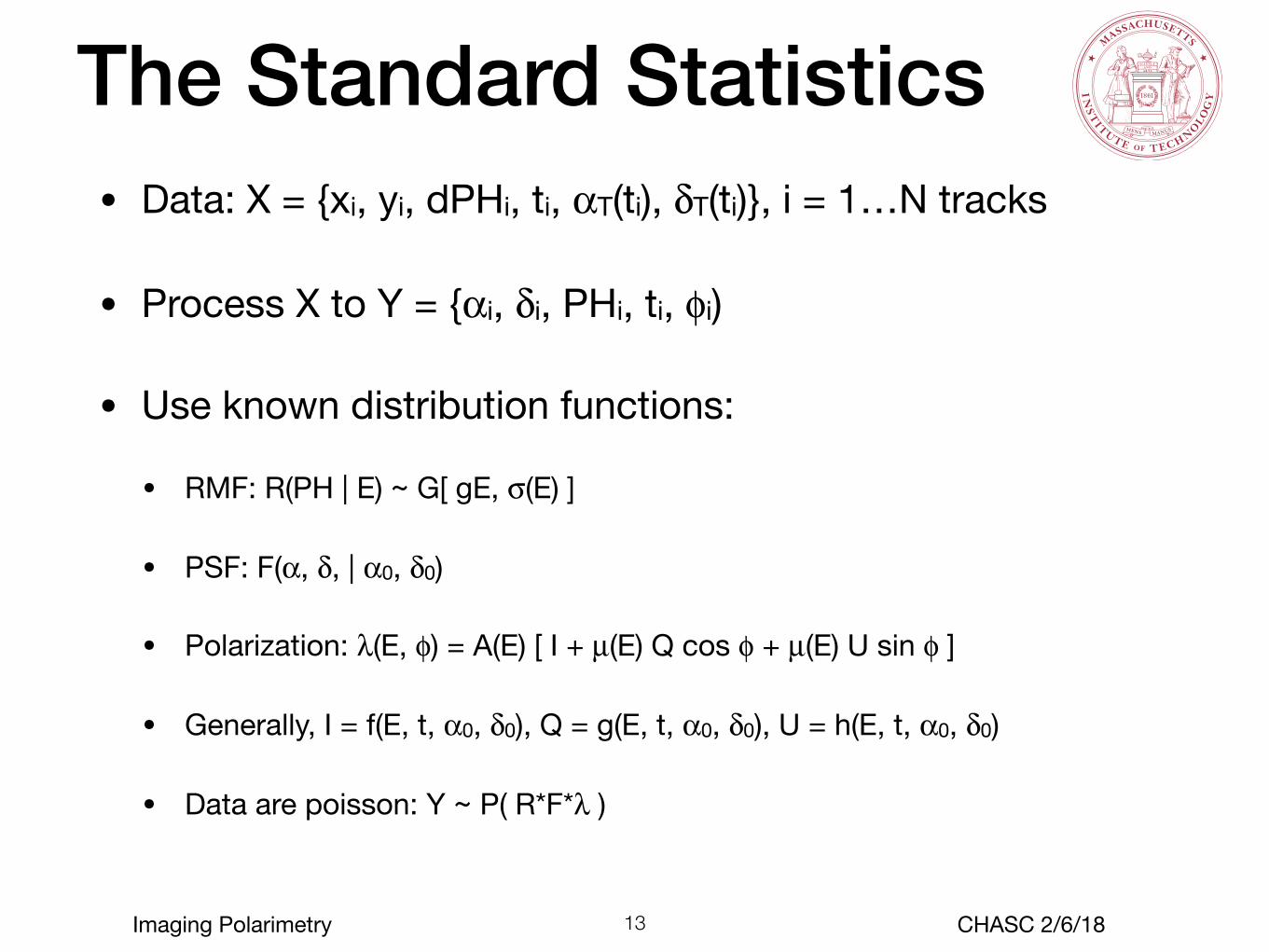
The Standard Statistics• Data: X = {xi, yi, dPHi, ti, aT(ti), dT(ti)}, i = 1…N tracks

• Process X to Y = {ai, di, PHi, ti, fi)

• Use known distribution functions:

• RMF: R(PH | E) ~ G[ gE, s(E) ]

• PSF: F(a, d, | a0, d0)

• Polarization: l(E, f) = A(E) [ I + µ(E) Q cos f + µ(E) U sin f ]

• Generally, I = f(E, t, a0, d0), Q = g(E, t, a0, d0), U = h(E, t, a0, d0)

• Data are poisson: Y ~ P( R*F*l )

13


Standard Analysis

14

With uncertainties, but qµ << 1, uµ << 1


Standard Analysis, Unbinned

15


The Track Problem• Track measurement is

empirical• Tracks have randomness

• Bulk of PH is at (uninteresting) end of track

• Low E tracks are short

• Some events are not considered

• Tracks are only probabilistically related to X-ray polarization

• Tracks are measured independently

16


Track Algorithm Optimization

• MDP ~ 1/( µ e1/2 )

• Algorithm has parameters that trade off µ and e for best µ e1/2

17


Simulated Data

18


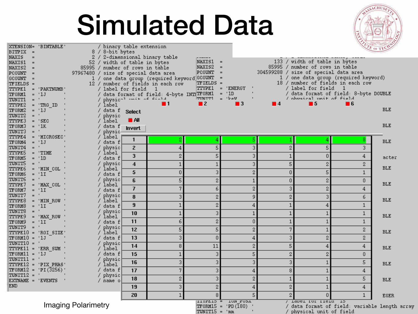
Simulated Data

19


Calibration Data

• Known:• polarization angle

• energy

• source position

• source is 100% polarized

• Detector data are ‘flight-like’

• Data are used to verify instrument model’s µ(E)

20


Track Measurement via Machine Learning

• Method 1 (‘Tracking’): Learn track directions• Only trains with simulated data, needs physics of interaction

• Event track is ~500 (x,y,PH) 3-tuples

• Simulations have known photoelectron direction

• Learns using ~10,000 events, apply to test sample of 1000 events

• Method 2 (‘Holistic’): Learn polarization of event list• Trains on either simulated or calibration data

• Training set is ~10,000 x 500 = 5 x 106 3-tuples

• Polarization direction is known for training, applied to test data

• Much faster than method 1

21

HLM, Adam Trebach (MIT) and Michelle Ntampaka (CfA)


Model Fitting• Traditional Method:

• Bin I on (t, E, a, d) into light curves, spectra, or images

• Fit binned (or perhaps unbinned event list) using response functions

• Handling complexity: time-dependent spectra, spatially varying spectra, etc: slice data in time or energy to make different spectra or images

• Problem: now add Q, U (or P, f)

• Assume P, f are independent of E or t —> use traditional methods

• Slice by E, a, d (or t, a, d) to get P(E), f(a, d), etc.

• Alternative: Use priors based on Chandra (if unvarying) or joint observations• Requires Bayesian, multi-parameter modeling

• Several scenarios are common

22


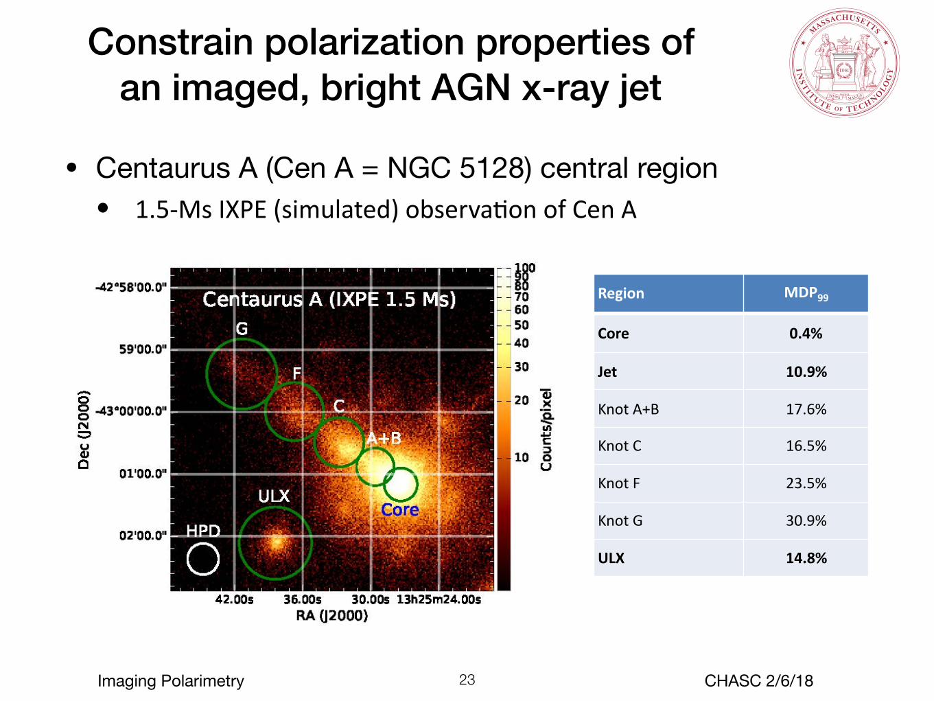
Constrain polarization properties of an imaged, bright AGN x-ray jet

• Centaurus A (Cen A = NGC 5128) central region• 1.5-MsIXPE(simulated)observaYonofCenA

23

Region MDP99

Core 0.4%

Jet 10.9%

KnotA+B 17.6%

KnotC 16.5%

KnotF 23.5%

KnotG 30.9%

ULX 14.8%


Model Testing

• Infeasible (?) using full track information• Tracks are not deterministically predictable

• Derive distributions of general properties of tracks?

• Simplistic, easy: bin data, use c2

• Feasible, easy: unbinned K-S on f, t, or E

• Challenging: Bayesian posterior

• Challenge: Simulation-based nearest neighbor test?

24

computational challenges from imaging x-ray polarimetry

Documents