computations with clifford and grassmann algebras · department of mathematics technical report...
TRANSCRIPT

DEPARTMENT OF MATHEMATICSTECHNICAL REPORT
COMPUTATIONS WITH CLIFFORDAND
GRASSMANN ALGEBRAS
RAFAL ABLAMOWICZ
MAY 2009
No. 2009-4
TENNESSEE TECHNOLOGICAL UNIVERSITYCookeville, TN 38505

Computations with Clifford and GrassmannAlgebras
Rafa l Ab lamowicz
Abstract. Various computations in Grassmann and Clifford algebras can beperformed with a Maple package CLIFFORD. It can solve algebraic equationswhen searching for general elements satisfying certain conditions, solve aneigenvalue problem for a Clifford number, and find its minimal polynomial. Itcan compute with quaternions, octonions, and matrices with entries in C`(B)- the Clifford algebra of a vector space V endowed with an arbitrary bilinearform B. It uses standard (undotted) Grassmann basis in C`(Q) but whenthe antisymmetric part of B is non zero, it can also compute in a dottedGrassmann basis. Some examples of computations are discussed.
Mathematics Subject Classification (2000). 15A66, 68W30.
Keywords. Quantum Clifford algebra, conformal group, contraction, dottedwedge product, grade involution, Grassmann algebra, Hopf algebra, multivec-tor, octonions, quaternions, reversion, singular value decomposition, spinors,Vahlen matrix, wedge product.
Contents
1. Introduction 22. Notation and Basic Computations 33. Clifford Product in C`(B) 94. Dotted and Undotted Grassmann Bases 12
4.1. The dotted wedge 124.2. Dotted and undotted wedge bases 134.3. Contraction and Clifford product in dotted and undotted bases 14
5. More on the Associativity of the Dotted Wedge 166. Reversion in Dotted and Undotted Bases 187. Spinor Representation of C`(Q) in Minimal Left Ideals 21
8. Two Scalar Products in Spinor Ideals 249. Continuous Families of Idempotents: Low Dimensional Examples 26

2 Rafa l Ab lamowicz
10. Vahlen Matrices 2811. Singular Value Decomposition and Clifford Algebra 3311.1. SVD of a 2 × 2 matrix of rank 2 34
11.2. Additional comments 4112. Conclusions 42Appendix A. Appendix: Code of cmulNUM 43Appendix B. Appendix: Code of cmulRS 44Appendix C. Appendix: Code of the Transposition Procedure tp 45References 46
1. Introduction
Some twenty years ago, late Professor Pertti Lounesto together with his colleaguesat Helsinki University of Technology developed CLICAL, a first semi-symbolic “Clif-ford algebra calculator”. [32] Along with it, Pertti brought to the world of Cliffordalgebraists a concept of experimental mathematics, algorithmic understanding, andcounter examples. [33] One could say that he was a pioneer in bringing togethertheoretical aspects and the computational part. His works, see for example [30],abound in concrete examples, and counter examples.
This author also believes that learning how mathematical concepts can behandled by a computer provides a combination of theory and practice that, as aresult, gives a better understanding of the theory of Clifford algebras and showshow the theory can be applied. This computational approach also provides a fastway to enter into the abstract field. We exemplify this approach by using a Maplepackage CLIFFORD, a system for computations with Grassmann polynomials, thatwas developed, like CLICAL, to support mathematical research in Grassmann andClifford algebras but using a full computer algebra system. [1, 8, 9]. More recently,this system was vastly extended with BIGEBRA for computations with tensors in ageneral setting of Hopf algebras and co-algebras. [9]
This approach of course is common to many other systems and fields thatbecame possible with the onset of fast computers capable of non-trivial symboliccomputations which had been intractable before by hand. For example, in thearea of commutative algebra one such system is provided by Singular [26] andanother by CoCoA [18]; in the area of algebraic geometry by Macaulay2 [36];and in the area of general mathematics, a category theory based AXIOM which isexplicitly “dedicated to research and development of mathematical algorithms”.[16] Finally, a review of existing software for Clifford algebras often developed witha specific computation in mind, can be found in [13].
A vector space V endowed with a quadratic form Q is common to a vasthost of mathematical, physical and engineering problems. This leads naturally toan algebra structure of the Clifford algebra C`(V,Q) and its generalization - aquantum Clifford algebra C`(V, B) for any bilinear form B. [6] This formalism, as

Computations with Clifford and Grassmann Algebras 3
compared to a standard vector calculus, can now be applied to solving completelynew problems. CLIFFORD was developed as a basic tool for all investigations andapplications which can be carried in finite dimensional vector spaces equippedwith a quadratic form or, equivalently, with a symmetric bilinear form commonlyreferred to as an inner or a scalar product. The intrinsic abilities of Maple evenallow one to use CLIFFORD in projective and affine geometries while visualizingcomplicated incidence relations that is helpful, e.g., for image processing, visualperception and robotics.
The authors of CLIFFORD and BIGEBRA have been interested in fundamen-tal questions about q-deformed symmetries and quantum field theory. Just askingquestions like such as “What is the most general element fulfilling . . . ?” has ledto unexpected results and new insights. [4,6,7,11] Checking the consistency of thesoftware by testing theorems and known results has led them in the foot stepsof Pertti Lounesto to counter examples that have made a rethinking and a morecareful restatement of those theorems necessary. However, the most striking abil-ity of CLIFFORD is that it is unique in being able to handle Clifford algebras ofan arbitrary bilinear form not restricted by symmetry and not directly related toany quadratic form. Since it is now well known that such structures are relatedto Hopf algebraic twists, later versions of CLIFFORD make an extensive use of aprocess called Rota-Stein cliffordization described in [20,22–25]. This, in turn, hasnecessitated introduction of a new algorithm based on this process for a more ef-ficient computation of the Clifford product in C`(V, B). As much as Buchberger’scelebrated algorithm is indispensable for computing Grobner bases, this new algo-rithm described in [9, 10] is indispensable for the Clifford product. Having devel-oped this faster algorithm one was able to find the q-Young Clifford idempotents[6] possessing a desired symmetry; explicitly describe the structure of the Spin(3)group; discover continuous families of idempotents in C`(Q) [11]; or gain a betterunderstanding of the properties of the dotted wedge product. [9]
The present paper brings to the reader a few examples of computations andresults derived with CLIFFORD. It is assumed that the reader is already familiarwith Maple [44], a general purpose CAS; if not please consult e.g., [45]. The articleis intended as a quick computational introduction to the abstract field of theClifford algebras, and, especially, to the field of quantum Clifford algebras. Forcomputations with tensor and Hopf algebras we refer to [10] that describes thesupplementary package BIGEBRA intended for such computations.
2. Notation and Basic Computations
CLIFFORD uses as default a standard Grassmann basis (Grassmann multivectors)in
∧
V where V = span {ei | 1 ≤ i ≤ n} for 1 ≤ n ≤ 9. Then
∧
V = span {ei ∧ ej ∧ . . . ∧ ek | 0 ≤ i < j < . . . < k ≤ n}.
4 Rafa l Ab lamowicz
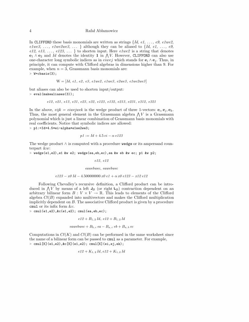
In CLIFFORD these basis monomials are written as strings {Id, e1, . . . , e9, e1we2,e1we3, . . . , e1we2we3, . . . } although they can be aliased to {Id, e1, . . . , e9,e12, e13, . . . , e123, . . . } to shorten input. Here e1we2 is a string that denotese1 ∧ e2 and Id denotes the identity 1 in
∧
V. However, CLIFFORD can also useone-character long symbolic indices as in eiwej which stands for ei ∧ ej. Thus, inprinciple, it can compute with Clifford algebras in dimensions higher than 9. Forexample, when n = 3, Grassmann basis monomials are:> W=cbasis(3);
W = [Id , e1 , e2 , e3 , e1we2 , e1we3 , e2we3 , e1we2we3 ]
but aliases can also be used to shorten input/output:> eval(makealiases(3));
e12 , e21 , e13 , e31 , e23 , e32 , e123 , e132 , e213 , e231 , e312 , e321
In the above, eijk = eiwejwek is the wedge product of three 1-vectors: ei, ej, ek.Thus, the most general element in the Grassmann algebra
∧
V is a Grassmannpolynomial which is just a linear combination of Grassmann basis monomials withreal coefficients. Notice that symbolic indices are allowed:> p1:=Id+4.5*ei-alpha*e1we2we3;
p1 := Id + 4.5 ei − α e123
The wedge product ∧ is computed with a procedure wedge or its ampersand coun-terpart &w:> wedge(e1,e2),e1 &w e2; wedge(ea,eb,ec),ea &w eb &w ec; p1 &w p2;
e12 , e12
eawebwec, eawebwec
e123 − x0 Id − 4.500000000 x0 e1 + α x0 e123 − x12 e12
Following Chevalley’s recursive definition, a Clifford product can be intro-duced in
∧
V by means of a left B (or right B) contraction dependent on anarbitrary bilinear form B : V × V → R. This leads to elements of the Cliffordalgebra C`(B) expanded into multivectors and makes the Clifford multiplicationimplicitly dependent on B. The associative Clifford product is given by a procedurecmul or its infix form &c.> cmul(e1,e2),&c(e1,e2); cmul(ea,eb,ec);
e12 + B1, 2 Id , e12 + B1, 2 Id
eawebwec + Bb, c ea − Ba, c eb +Ba, b ec
Computations in C`(K) and C`(B) can be performed in the same worksheet sincethe name of a bilinear form can be passed to cmul as a parameter. For example,> cmul[K](e1,e2),&c[K](e1,e2); cmul[K](ei,ej,ek);
e12 +K1, 2 Id , e12 + K1,2 Id
Computations with Clifford and Grassmann Algebras 5
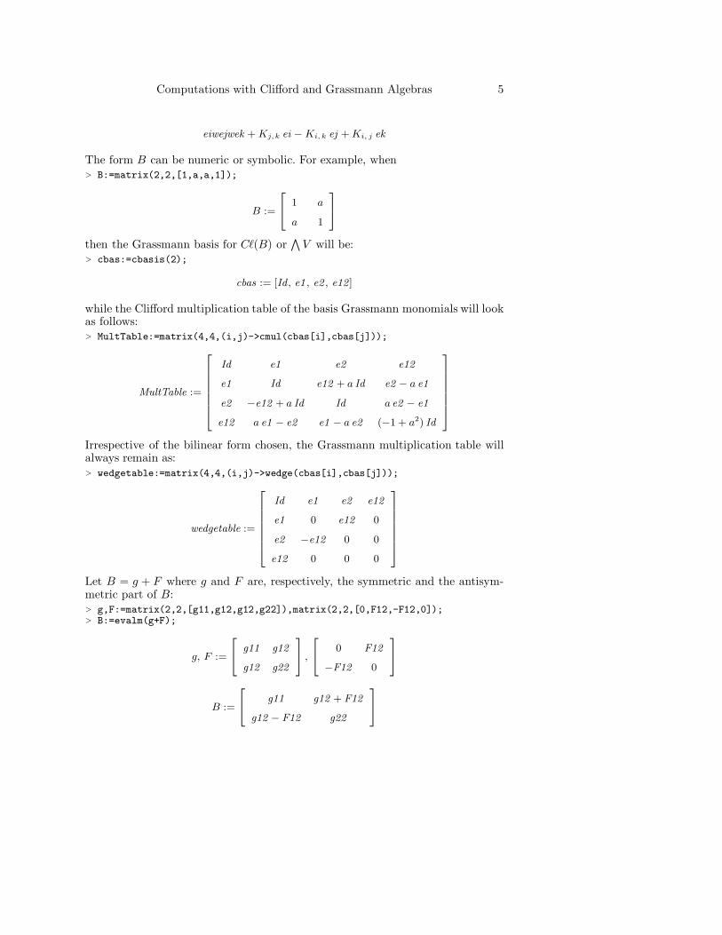
eiwejwek + Kj,k ei −Ki, k ej +Ki, j ek
The form B can be numeric or symbolic. For example, when> B:=matrix(2,2,[1,a,a,1]);
B :=
2
4
1 a
a 1
3
5
then the Grassmann basis for C`(B) or∧
V will be:> cbas:=cbasis(2);
cbas := [Id , e1 , e2 , e12 ]
while the Clifford multiplication table of the basis Grassmann monomials will lookas follows:> MultTable:=matrix(4,4,(i,j)->cmul(cbas[i],cbas[j]));
MultTable :=
2
6
6
6
6
6
6
4
Id e1 e2 e12
e1 Id e12 + a Id e2 − a e1
e2 −e12 + a Id Id a e2 − e1
e12 a e1 − e2 e1 − a e2 (−1 + a2) Id
3
7
7
7
7
7
7
5
Irrespective of the bilinear form chosen, the Grassmann multiplication table willalways remain as:> wedgetable:=matrix(4,4,(i,j)->wedge(cbas[i],cbas[j]));
wedgetable :=
2
6
6
6
6
6
6
4
Id e1 e2 e12
e1 0 e12 0
e2 −e12 0 0
e12 0 0 0
3
7
7
7
7
7
7
5
Let B = g + F where g and F are, respectively, the symmetric and the antisym-metric part of B:> g,F:=matrix(2,2,[g11,g12,g12,g22]),matrix(2,2,[0,F12,-F12,0]);> B:=evalm(g+F);
g, F :=
2
4
g11 g12
g12 g22
3
5 ,
2
4
0 F12
−F12 0
3
5
B :=
2
4
g11 g12 + F12
g12 − F12 g22
3
5

6 Rafa l Ab lamowicz
Then, the Clifford multiplication table of the basis monomials in C`(B) will be asfollows:> MultTable:=matrix(4,4,(i,j)->cmul(cbas[i],cbas[j]));
MultTable := [Id , e1 , e2 , e12 ]
[e1 , g11 Id , e12 + (g12 + F12 ) Id , g11 e2 − (g12 + F12) e1 ]
[e2 , (g12 − F12) Id − e12 , g22 Id , (g12 − F12) e2 − g22 e1 ]
[e12 , (g12 − F12) e1 − g11 e2 , g22 e1 − (g12 + F12) e2 ,
(g122 − F122 − g22 g11) Id − 2 e12 F12 ]
Observe, that the “standard” anticommutation relations
eiej + ejei = (Bi,j +Bj,i)1 = 2gi,j1 (1)
are satisfied by the generators ei, i = 1, 2, . . . , n, irrespective of the presence ofthe antisymmetric part F in B. For example,> cmul[g](e1,e2)+cmul[g](e2,e1);> cmul[B](e1,e2)+cmul[B](e2,e1);
2 Id g12
(g12 + F12) Id + (g12 − F12 ) Id = 2 g12 Id
It is well known [29, 35] that real Clifford algebras C`(V,Q) = C`p,q areclassified in terms of the signature (p, q) of Q and the dimension dimV = n = p+q.Information about all Clifford algebras C`p,q, 1 ≤ n ≤ 9, for any signature (p, q)has been pre-computed and stored in CLIFFORD, and it can be retrieved with aprocedure clidata. For example, for the Clifford algebra C`2,0 (also denoted asC`2) of the Euclidean plane R2 we find:> clidata([2,0]); #Clifford algebra of the Euclidean plane
[real , 2, simple,1
2Id +
1
2e1 , [Id , e2 ], [Id ], [Id , e2 ]]
The meaning of the first three entries in the above output list is that C`2 is asimple algebra isomorphic to Mat(2,R). The 4th entry in the list gives a primitiveidempotent f that has been used to generate a minimal left spinor ideal S = C`2fand, subsequently, the left spinor (lowest dimensional and faithful) representationof C`2 in S. In general it is known that, depending on (p, q) and n = dimV, thespinor ideal S = C`p,qf is a right K-module where K is either R,C, or H for simpleClifford algebras when (p − q) 6= 1 mod 4, or R ⊕ R and H ⊕ H for semisimplealgebras when (p−q) = 1 mod 4. [27,30] Elements in the 5th entry (here [Id , e2 ])generate a real basis in S with respect to f, that is, S = span {Id &c f, e2 &c f} =span {f, e2 &c f}. Elements in the 6th entry span a subalgebra F of C`(Q) thatis isomorphic to K. In the case of C`2 we find that F = span {Id} ∼= R. Thelast entry in the output gives 2k generators of S (with respect to f) viewed as aright module over K where k = q − rq−p and r is the Radon-Hurwitz number.1
Number k is the number of factors 12 (1 + Ti), where {Ti}, i = 1, . . . , k, is a set of
commuting basis Grassmann monomials squaring in C`(Q) to 1, whose productgives a primitive idempotent f in C`(Q). Spinor representation for all Clifford
1Type ?RHnumber in a Maple session when CLIFFORD is installed for more help.

Computations with Clifford and Grassmann Algebras 7
algebras C`(Q), 1 ≤ n = p + q ≤ 9, and for any signature (p, q) has been pre-computed [3] and can be retrieved from CLIFFORD with a procedure matKrepr.For example, 1-vectors e1 and e2 in C`2 have the following spinor representationin the basis {f, e2 &c f} of S = C`2f :2
> matKrepr([2,0]);
[e1 =
2
4
1 0
0 −1
3
5 , e2 =
2
4
0 1
1 0
3
5]
In another example, Clifford algebra C`3 of R3 is isomorphic with Mat(2,C):> B:=linalg[diag](1,1,1):clidata([3,0]);
[complex, 2, simple,1
2Id +
1
2e1 , [Id, e2 , e3 , e23 ], [Id , e23 ], [Id , e2 ]]
and its spinor representation is given in terms of Pauli matrices:> matKrepr([3,0]);
[e1 =
2
4
1 0
0 −1
3
5 , e2 =
2
4
0 1
1 0
3
5 , e3 =
2
4
0 −e23
e23 0
3
5]
Notice that F = span {Id , e23} (e23 = e2we3 ) is a subalgebra of C`3 isomorphicto C. Since Pauli matrices belong to Mat(2, F ), it is necessary for CLIFFORD tocompute with Clifford matrices, that is, matrices of a type ‘type/climatrix‘with entries in a Clifford algebra.> M1,M2,M3:=rhs(%[1]),rhs(%[2]),rhs(%[3]);
M1 , M2 , M3 :=
2
4
1 0
0 −1
3
5 ,
2
4
0 1
1 0
3
5 ,
2
4
0 −e23
e23 0
3
5 .
Of course Pauli matrices satisfy the same defining relations as the basis vectorse1, e2, and e3:3 For example:> ‘M1 &cm M2 + M2 &cm M1‘ = evalm(M1 &cm M2 + M2 &cm M1);> ‘e1 &c e2 + e2 &c e1‘=e1 &c e2 + e2 &c e1;
M1 &cm M2 + M2 &cm M1 =
2
4
0 0
0 0
3
5
e1 &c e2 + e2 &c e1 = 0
2We use the sloppy notation 1 ≡ 1 in Clifford algebra valued matrices which produces a simplerdisplay.3Here &cm is a matrix product where Clifford multiplication is applied to the matrix entries.
See ?&cm for more information.

8 Rafa l Ab lamowicz
> ‘M1 &cm M1‘ = evalm(M1 &cm M1),‘M2 &cm M2‘ = evalm(M2 &cm M2),> ‘M3 &cm M3‘ = evalm(M3 &cm M3);> ‘e1 &c e1‘ = e1 &c e1,‘e2 &c e2‘ = e2 &c e2,‘e3 &c e3‘ = e3 &c e3;
M1 &cm M1 =
2
4
1 0
0 1
3
5 ,M2 &cm M2 =
2
4
1 0
0 1
3
5 ,M3 &cm M3 =
2
4
1 0
0 1
3
5
e1 &c e1 = Id , e2 &c e2 = Id , e3 &c e3 = Id
The procedure matKrepr gives the linear isomorphism C`(Q) ' Mat(2,R), and,in general, C`(Q) ' Mat(2k, K), where K = R,C,H, for simple algebras andC`(Q) ' Mat(2k, K) ⊕ Mat(2k, K), where K = R,H, for semisimple algebras. Inthis latter case, it is customary to represent an element in C`(Q) in terms of asingle matrix over a double field R⊕R or H⊕H rather than as pair of matrices.4
One can easily list signatures of the quadratic form Q for which C`(Q) issimple or semisimple. For more information, type ?all sigs. For example, C`1,3
has a spinor representation given in terms of 2 by 2 quaternionic matrices whoseentries belong to a subalgebra F of C`1,3 spanned by {Id , e2 , e3 , e2we3}:> B:=linalg[diag](1,-1,-1,-1):clidata([1,3]);
[quaternionic, 2, simple,1
2Id +
1
2e1we4 , [Id , e1 , e2 , e3 , e12 , e13 , e23 , e123 ],
[Id , e2 , e3 , e23 ], [Id , e1 ]]
> matKrepr([1,3]); #quaternionic matrices
[e1 =
2
4
0 1
1 0
3
5 , e2 =
2
4
e2 0
0 −e2
3
5 , e3 =
2
4
e3 0
0 −e3
3
5 , e4 =
2
4
0 −1
1 0
3
5]
CLIFFORD includes several special-purpose procedures to deal with quaternionsand octonions (type ?quaternion and ?octonion for help), and with quaternionicand octonionic matrices. In particular, following [32], octonions are treated as para-vectors in C`0,7 while their non-associative multiplication, defined via Fano triples,is related to the Fano projective plane F2 (see ?omultable, or ?Fano triples formore information). User can select different Fano triples and redefine the octo-nionic multiplication table. Since the bilinear form B can be degenerate5 , one canuse CLIFFORD to perform computations in Clifford algebras C`p,q,d of a degeneratequadratic form Q of signature (p, q) and the dimension d of its radical. For exam-ple, the Clifford algebra C`0,3,1 of the quadratic form Q(x) = −x2
1−x22 −x2
3 wherex = x1e1 + x2e2 + x3e3 + x4e4 ∈ R4 is used in robotics to represent rigid motionsin R3 and screw motions in terms of dual quaternions. [4, 41]
Thus, CLIFFORD is a repository of mathematical knowledge about Cliffordalgebras of a quadratic form in dimensions 1 through 9. Together with a sup-plementary package BIGEBRA [8] it can be extended to graded tensor products of
4Procedures adfmatrix and mdfmatrix add and multiply matrices of type dfmatrix over such
double fields. For more information see ?matKrepr.5When B ≡ 0 then C`(V,B) = C`0,0,n =
V
V and computations in the Grassmann algebraV
V
can then be done with CLIFFORD.

Computations with Clifford and Grassmann Algebras 9
Clifford algebras in higher dimensions. The BIGEBRA package is described in [10].For more information about any CLIFFORD or BIGEBRA procedure, type ?Cliffordor ?Bigebra to see its top level help page in the Maple browser. For a computationof spinor representations with CLIFFORD we refer to [3].
3. Clifford Product in C`(B)
The Clifford product in a Clifford algebra C`(B) of an arbitrary bilinear form B isintroduced via the Chevalley deformation and the Clifford map. [35] The Cliffordmap γx is defined on u ∈ ∧
V as
(i) γx(u) = LC(x, u, B) + wedge(x, u) = x B u+ x ∧ u(ii) γxγy = γx∧y +B(x,y)γ1(iii) γax+by = aγx + bγy
where x,y ∈ V (see, for example, [35]). One knows how to compute with the wedgex∧u and the left contraction x B u of u by x with respect to the bilinear form B.6
Following Chevalley, the left contraction has the following properties:
(i) x B y = B(x,y)(ii) x B (u ∧ v) = (x B u) ∧ v + u ∧ (x B v)(iii) (u ∧ v) B w = u B (v B w)
where x ∈ V, u, v ∈ ∧
V and u is the Grassmann grade involution. Hence wecan use the Clifford map γx (Chevalley deformation of the Grassmann algebra) todefine a Clifford product of a one-vector x and a multivector u as
xu = x B u+ x ∧ u. (2)
Analogous formula can also be given for a right Clifford map using the rightcontraction B implemented as the procedure RC.
The Clifford product cmul or its ampersand form &c of two Grassmann basismonomials can now be defined as follows: A single element from the first factor ofthe product is split off recursively and then the Chevalley’s Clifford map is applied.Namely,
(ea ∧ . . .∧ eb ∧ ec)&c(ef ∧ . . . ∧ eg) =
(ea ∧ . . . ∧ eb)&c(ec B (ef ∧ . . .∧ eg) + ec ∧ ef ∧ . . .∧ eg)
− ((ea ∧ . . . ∧ eb) B ec)&c(ef ∧ . . . ∧ eg). (3)
Specifically, for (e1 ∧ e2)&c(e3 ∧ e4) we have
(e1 ∧ e2)&c(e3 ∧ e4) = (e1&ce2)&c(e3 ∧ e4) −B(e1, e2)1&c(e3 ∧ e4)
= e1&c(B(e2, e3)e4 −B(e2, e4)e3 + e2 ∧ e3 ∧ e4)
−B(e1, e2)1&c(e3 ∧ e4)
6In CLIFFORD, the left contraction B is given by the procedure LC(x, u, B), or, simply, by LC(x, u)where B is assumed as default. The right contraction u B x of u by x is encoded as a procedure
RC(u, x, B), or simply RC(u, x).

10 Rafa l Ab lamowicz
and the second recursion of the process gives now
= B(e2, e3)B(e1 , e4) − B(e2, e4)B(e1, e3) + B(e2, e3)(e1 ∧ e4)
−B(e2 , e4)(e1 ∧ e3) + B(e1, e2)(e3 ∧ e4) − B(e1, e3)(e2 ∧ e4)
+B(e1 , e4)(e2 ∧ e3) + e1 ∧ e2 ∧ e3 ∧ e4 −B(e1, e2)(e3 ∧ e4)
with the bold terms canceling out. Note that the last term in the r.h.s. was super-fluously generated in the first step of the recursion.
The Clifford product can then be derived from the above recursion by linear-ity and associativity. The induction starts with a left factor of grade one or gradezero which is trivial, i.e., 1 &c ea ∧ . . .∧eb = ea ∧ . . .∧eb. In the case when the leftfactor is of grade one, we use the Clifford product expressed by the Clifford mapof Chevalley, i.e.,
ea &c eb ∧ . . .∧ ec = ea B (eb ∧ . . . ∧ ec) + ea ∧ eb ∧ . . . ∧ ec.
We make a complete induction in the following way: If the left factor is of highergrade, say n, one application of the recursion yields Clifford products where thenew left factor is of grade either n− 1 or n− 2, hence the recursion stops after atmost n− 1 steps.
The above shows clearly that both the Clifford product and the contrac-tion are explicitly dependent on B. Furthermore, the Clifford product algorithmbased on the Chevalley’s approach is recursive. It has been encoded in a procedurecmulNUM (see Appendix A).
Since the Clifford product provides the main functionality of the CLIFFORD
package, care has been exercised to select the most appropriate and sound mathe-matics. Two internal user-selectable functions cmulNUM and cmulRS, an algorithmbased on a combinatorial approach due to Rota and Stein, have been used to en-code the Clifford product but the user normally does not use either one. Instead,the user uses a wrapper function &c[K](arg1 , arg2 , . . .) or cmul[K](arg1 , arg2 , . . .)that passes the name of a bilinear form K to either cmulRS or cmulNUM, whicheverone has been selected to act on the multivector basis monomials. This approachallows the user to compute in the same worksheet simultaneously with differentClifford algebras of different bilinear forms. The wrapper function can also acton any number of arguments of type ‘type/clipolynom‘ as the Clifford productis associative and on a much wider class of types including Clifford matrices oftype ‘type/climatrix‘. It can also accept Clifford polynomials in other basessuch as the Clifford basis {1, ei, ei &C ej,&C(ei, ej, ek), . . .} where &C denotes theunevaluated Clifford product. Clifford basis differs from the Grassmann exteriorbasis when B is not a diagonal matrix.7
7Procedures converting between Grassmann and Clifford bases belong to a supplementarypackage Cliplus [8] while Clifford polynomials expressed in the Clifford basis are of type
‘type/cliprod‘. Type ?cliprod for more information.

Computations with Clifford and Grassmann Algebras 11
The procedure cmulRS is encoded a non-recursive Rota-Stein cliffordization.See [10, 20, 22, 24, 40] and BIGEBRA help pages for additional references.8 The clif-fordization process is based on the Hopf algebra theory. The Clifford product isobtained from the Grassmann wedge product and its Grassmann co-product asshown by the following tangle:
&c :=
∆∧ ∆∧B∧
∧(4)
Here ∧ is the Grassmann exterior wedge product and ∆∧ is the Grassmann exteriorco-product which is obtained from the wedge product by a categorial duality: Toevery algebra over a linear space A with a product we find a co-algebra with a co-product over the same space by reversing all arrows in all axiomatic commutativediagrams. Note that the co-product splits each input ‘factor’ x into a sum oftensor products of ordered pairs x(1)i, x(2)i. The main requirement is that everysuch pair multiplies back to the input x when the dual operation of multiplicationis applied, i.e., x(1)i ∧ x(2)i = x for each i-th pair. The ‘cup’ like part of the tangledecorated with B∧ is the bilinear form B on the generating space V extended tothe whole Grassmann algebra: It is a map B∧ :
∧
V ×∧
V → k with B : V ×V → k
evaluating to B(x,y) on vectors in V. Hence, cmulRS computes the Clifford producton Grassmann basis monomials x and y for the given B, which is later extendedto Clifford polynomials by bilinearity, as follows:
cmulRS(x, y, B) =
n∑
i=1
m∑
j=1
(±)x(1)i ∧ y(2)jB(x(2)i, y(1)j) (5)
where n and m give the cardinalities of the required splits and the sign is due tothe parity of a permutation needed to arrange the factors.
After reviewing the code of cmulRS given in Appendix B it becomes clearthat in this algorithm only those terms are created which might be non-zero andare likely to remain in the final result: If all Bi,j are non-zero and different sothat no cancellation takes place, only exactly those terms will be returned. Yet, nosuperfluous terms are created like in the recursive procedure cmulNUM that laterare canceled in subsequent recursive steps. The combinatorial power of the Hopfalgebraic approach is clearly demonstrated with this algorithm and its superiorbehavior shows up in benchmarks. [9, 10]
8BIGEBRA is an extension of CLIFFORD and was specifically developed to work with Hopf alge-
bras. [8]

12 Rafa l Ab lamowicz
The two internal Clifford multiplication procedures along with their advan-tages and disadvantages are discussed in [9]. It should suffice to say here thatcmulNUM is fast on sparse numeric matrices and on numeric matrices in generalwhen dimV ≥ 5, while the procedure cmulRS was designed for high efficiency withsymbolic calculations.
4. Dotted and Undotted Grassmann Bases
4.1. The dotted wedge
The dotted wedge product was introduced by Lounesto. [35] Clifford algebras withthe dotted and the undotted wedge products are isomorphic. It turns out that invarious situations, i.e., in quantum field theory or in a representation theory, one isinterested in studying isomorphic but not identical algebras in which mathematicalobjects can be expressed in different bases such as the dotted and the undottedwedge bases. [9]
It was shown above that CLIFFORD uses the Grassmann algebra∧
V as theunderlying vector space of the Clifford algebra C`(V, B). Thus, the Grassmannwedge basis of monomials is the standard basis used in CLIFFORD. A general ele-ment u in C`(V, B) can be therefore viewed as a Grassmann polynomial.
When the bilinear form B has an antisymmetric part F = −F T , it is conve-nient to split it as B = g+F, where g is the symmetric part of B, and to introducethe so called “dotted Grassmann basis” [12] and the dotted wedge product ∧. Theoriginal Grassmann basis will be referred to here as the “undotted Grassmannbasis”. In CLIFFORD, the wedge product is given by the procedure wedge and &wwhile the dotted wedge product is given by dwedge and &dw.
According to Chevalley’s definition of the Clifford product &c, we have
x &c u = x B u+ x &wu = LC(x, u, B) + wedge(x, u) (6)
for a 1-vector x and an arbitrary element u of C`(B). As before, LC(x, u, B) denotesthe left contraction of u by x with respect to the bilinear form B. However, whenB = g + F then the left contraction splits too:
x B u = LC(x, u, B) = x g u+ x F u = LC(x, u, g) + LC(x, u, F ) (7)
and
x &cu = LC(x, u, B) + x &wu (8)
= LC(x, u, g) + LC(x, u, F ) + x &w u (9)
= LC(x, u, g) + dwedge[F ](x, u) = LC(x, u, g) + x &dw u (10)
where x &dwu = x &wu + LC(x, u, F ). That is, the wedge and the dotted wedge“differ” by the contraction term(s) with respect to the antisymmetric part F of B.This dotted wedge &dw can be extended to elements of higher grades. Its propertiesare discussed next.
Procedure dwedge (and its infix form &dw) requires an index which can be asymbol or an antisymmetric matrix. That is, dwedge computes the dotted wedge

Computations with Clifford and Grassmann Algebras 13
product of two Grassmann polynomials and expresses its answer in the undottedbasis. Special procedures exist which convert polynomials between the undottedand dotted bases. When no index is used, the default is F :> dwedge[K](e1+2*e2we3,e4+3*e1we2);&dw(ei+2*ejwek,ei+2*ejwek);
−(−K1,4 + 6K2,3K1, 2) Id − 6K1, 2 e2we3 − 6K2,3 e1we2
−2K2, 4 e3 + 2K3, 4 e2 − 3K1, 2 e1 + e1we4 + 2 e2we3we4
4 eiwejwek − 4Fi, k ej + 4Fi, j ek − 8Fj, k ejwek − 4Fj, k2 Id
Observe that conversion from the undotted wedge basis to the dotted wedge ba-sis using antisymmetric form F and dwedge[F] are related through the followingconvert function:
dwedge[F ](e1, e2, ..., en) = convert(e1we2w ...wen, wedge to dwedge, F )
which can be shown as follows:> F:=array(1..9,1..9,antisymmetric):> dwedge[F](e1,e2)=convert(wedge(e1,e2),wedge_to_dwedge,F);
e1we2 + F1, 2 Id = e1we2 + F1,2 Id
> dwedge[F](e1,e2,e3)=convert(wedge(e1,e2,e3),wedge_to_dwedge,F);
e1we2we3 + F2, 3 e1 − F1,3 e2 + F1, 2 e3 = e1we2we3 + F2, 3 e1 − F1,3 e2 + F1, 2 e3
C`(B)∧ C`(B)∧
wedge to dwedge
dwedge to wedge
Diagram 1. Isomorphisms between C`(B)∧ and C`(B)∧.
For a more complete treatment see [9].
4.2. Dotted and undotted wedge bases
Symbolic capabilities of the computer algebra system allow for an investigation ofproperties of the Clifford product, contraction, and the reversion in the dotted andthe undotted bases. In this way, the CAS allows for a better understanding of thesefundamental to any Clifford algebra C`(B) operations. Here we show only a fewfacts and refer to [9,10]. For example, we expand the basis of the original wedge intothe dotted wedge, and back using the two conversion functions mentioned above.For this purpose we choose dimV = 3 and consider C`(B) with the antisymmetricpart F. The undotted wedge basis for
∧
V is then:> w_bas:=cbasis(dim_V); #the wedge basis
w bas := [Id , e1 , e2 , e3 , e1we2 , e1we3 , e2we3 , e1we2we3 ]

14 Rafa l Ab lamowicz
Now we map the convert function onto this basis to get the dotted wedge basis:> d_bas:=map(convert,w_bas,wedge_to_dwedge,F);> test_wbas:=map(convert,d_bas,dwedge_to_wedge,-F);
d bas := [Id , e1 , e2 , e3 , e1we2 + F1,2 Id , e1we3 + F1, 3 Id , e2we3 + F2, 3 Id ,
e1we2we3 + F2,3 e1 − F1, 3 e2 + F1, 2 e3 ]
test wbas := [Id , e1 , e2 , e3 , e1we2 , e1we3 , e2we3 , e1we2we3 ]
Notice that only the unity 1 and the one vector basis elements ei remain unalteredand that the other basis elements of higher grades pick up additional terms oflower grades (which preserves the filtration). It is possible to define aliases inCLIFFORD for the dotted wedge basis “monomials” similar to the Grassmann basismonomials. For example, we could denote the element e1we2 + F [1 , 2 ] ∗ Id bye1We2 (= e1 ∧ e2) and similarly for other elements:> alias(e1We2=e1we2 + F[1,2]*Id,e1We3=e1we3 + F[1,3]*Id,> e2We3=e2we3 + F[2,3]*Id,> e1We2We3=e1we2we3+F[2,3]*e1-F[1,3]*e2+F[1,2]*e3);
I, e1We2 , e1We3 , e2We3 , e1We2We3
and then Maple will automatically display dotted basis in terms of the aliases:> d_bas;
[Id , e1 , e2 , e3 , e1We2 , e1We3 , e2We3 , e1We2We3 ]
That is, as linear spaces we find the isomorphism:
C`(B) ∼= 〈1, e1, e2, e3, e1 ∧ e2, e1 ∧ e3, e2 ∧ e3, e1 ∧ e2 ∧ e3〉∼= 〈1, e1, e2, e3, e1 ∧ e2, e1 ∧ e3, e2 ∧ e3, e1 ∧ e2 ∧ e3〉
where e1 ∧ e2 = e1We2 , etc.
4.3. Contraction and Clifford product in dotted and undotted bases
For details we refer to [9]. The contraction B w.r.t. any bilinear form B works onboth undotted and dotted bases in a consistent and essentially the same manner ascan be see from the next diagram which utilizes the conversion functions betweenthe two bases. Let F be the antisymmetric part of B. To read more about theleft contraction LC in C`(B) check the help page for LC or see [12]. We have thefollowing identity for any two elements u and v in C`(B) expressed in the undottedGrassmann basis:
v B u = (v B uF )−F (11)
As before, uF is the element u expressed in the dotted basis while (. . .)−F accom-plishes conversion back to the undotted basis. To illustrate this fact, we first con-tract from the left an arbitrary element u in C`(B) by 1, ei, ei∧ej, ei∧ej∧ek, 1 ≤i, j, k ≤ 3 (here we limit our example to dimV = 3) and then we extend it to aleft contraction by an arbitrary element v in C`(B).> u:=add(x.i*w_bas[i+1],i=0..7):uF:=convert(uw,wedge_to_dwedge,F):> v:=add(y.i*w_bas[i+1],i=0..7):Contraction with respect to 1:> evalb(LC(Id,u,B)=convert(LC(Id,uF,B),dwedge_to_wedge,-F));

Computations with Clifford and Grassmann Algebras 15
C`(B)∧ ⊗ C`(B)∧ C`(B)∧ ⊗C`(B)∧
C`(B)∧ C`(B)∧
1⊗ (. . .)F
B B
(. . .)−F
Diagram 2. Contraction w.r.t. wedge and dotted wedge.
true
Contraction with respect to ei:> evalb(LC(ei,u,B)=convert(LC(ei,uF,B),dwedge_to_wedge,-F));
true
Contraction with respect to ei ∧ ej:> evalb(LC(eiwej,u,B)=convert(LC(eiwej,uF,B),dwedge_to_wedge,-F));
true
Contraction with respect to ei ∧ ej ∧ ek:> evalb(LC(eiwejwek,u,B)=convert(LC(eiwejwek,uF,B),dwedge_to_wedge,-F));
true
Finally, contraction with respect to an arbitrary element v:> evalb(LC(v,u,B)=convert(LC(v,uF,B),dwedge_to_wedge,-F));
true
Once we have the dotted and the undotted Grassmann bases, we can build aClifford algebra C`(B) over each basis set but with different bilinear forms: B = gor B = g + F respectively (following notation from [12]). Let us compute variousClifford products with respect to the symmetric form g and with respect to thefull form B using procedure cmul that takes a bilinear form as its index. As anexample, we will use two most general elements u and v in
∧
V when dimV = 3.Most output will be eliminated.> u:=add(x.k*w_bas[k+1],k=0..7):v:=add(y.k*w_bas[k+1],k=0..7):We can then define in
∧
V a Clifford product cmul[g] with respect to the sym-metric part g and another Clifford product cmul[B] with respect to the entireform B:> cmulg:=proc() return cmul[g](args) end proc:> cmulB:=proc() return cmul[B](args) end proc:
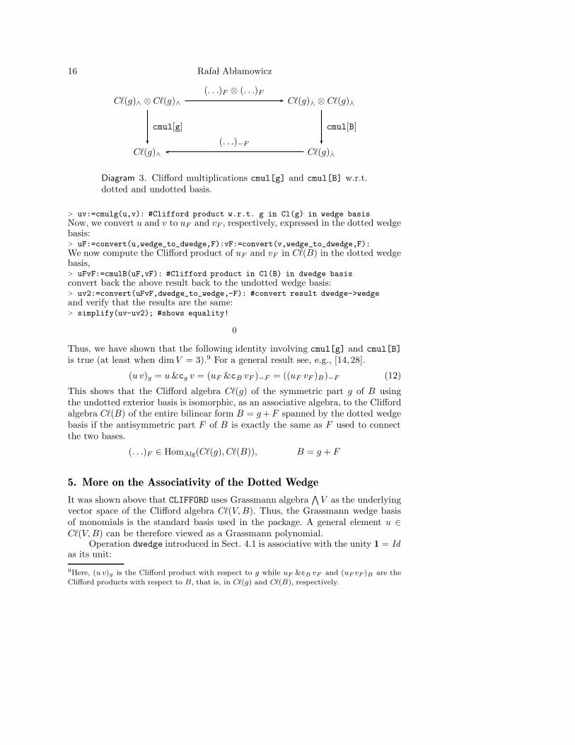
We will illustrate relation between the two Clifford products by chasing the follow-ing commutative diagram, however most output will be eliminated to save space.
First, we compute the Clifford product cmul[g](u, v) in C`(g) in undotted Grass-mann basis.
16 Rafa l Ab lamowicz
C`(g)∧ ⊗C`(g)∧ C`(g)∧ ⊗ C`(g)∧
C`(g)∧ C`(g)∧
(. . .)F ⊗ (. . .)F
cmul[g] cmul[B]
(. . .)−F
Diagram 3. Clifford multiplications cmul[g] and cmul[B] w.r.t.dotted and undotted basis.
> uv:=cmulg(u,v): #Clifford product w.r.t. g in Cl(g) in wedge basisNow, we convert u and v to uF and vF , respectively, expressed in the dotted wedgebasis:> uF:=convert(u,wedge_to_dwedge,F):vF:=convert(v,wedge_to_dwedge,F):We now compute the Clifford product of uF and vF in C`(B) in the dotted wedgebasis,> uFvF:=cmulB(uF,vF): #Clifford product in Cl(B) in dwedge basisconvert back the above result back to the undotted wedge basis:> uv2:=convert(uFvF,dwedge_to_wedge,-F): #convert result dwedge->wedgeand verify that the results are the same:> simplify(uv-uv2); #shows equality!
0
Thus, we have shown that the following identity involving cmul[g] and cmul[B]
is true (at least when dimV = 3).9 For a general result see, e.g., [14, 28].
(u v)g = u&cg v = (uF &cB vF )−F = ((uF vF )B)−F (12)
This shows that the Clifford algebra C`(g) of the symmetric part g of B usingthe undotted exterior basis is isomorphic, as an associative algebra, to the Cliffordalgebra C`(B) of the entire bilinear form B = g+F spanned by the dotted wedgebasis if the antisymmetric part F of B is exactly the same as F used to connectthe two bases.
(. . .)F ∈ HomAlg(C`(g), C`(B)), B = g + F
5. More on the Associativity of the Dotted Wedge
It was shown above that CLIFFORD uses Grassmann algebra∧
V as the underlyingvector space of the Clifford algebra C`(V, B). Thus, the Grassmann wedge basisof monomials is the standard basis used in the package. A general element u ∈C`(V, B) can be therefore viewed as a Grassmann polynomial.
Operation dwedge introduced in Sect. 4.1 is associative with the unity 1 = Idas its unit:
9Here, (u v)g is the Clifford product with respect to g while uF &cB vF and (uF vF )B are the
Clifford products with respect to B, that is, in C`(g) and C`(B), respectively.
Computations with Clifford and Grassmann Algebras 17
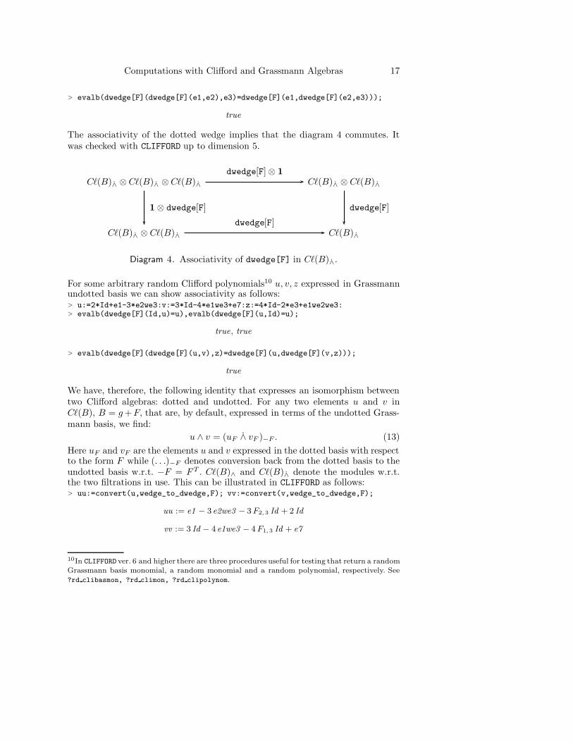
> evalb(dwedge[F](dwedge[F](e1,e2),e3)=dwedge[F](e1,dwedge[F](e2,e3)));
true
The associativity of the dotted wedge implies that the diagram 4 commutes. Itwas checked with CLIFFORD up to dimension 5.
C`(B)∧ ⊗C`(B)∧ ⊗C`(B)∧ C`(B)∧ ⊗ C`(B)∧
C`(B)∧ ⊗ C`(B)∧ C`(B)∧
dwedge[F] ⊗ 1
1⊗ dwedge[F] dwedge[F]
dwedge[F]
Diagram 4. Associativity of dwedge[F] in C`(B)∧.
For some arbitrary random Clifford polynomials10 u, v, z expressed in Grassmannundotted basis we can show associativity as follows:> u:=2*Id+e1-3*e2we3:v:=3*Id-4*e1we3+e7:z:=4*Id-2*e3+e1we2we3:> evalb(dwedge[F](Id,u)=u),evalb(dwedge[F](u,Id)=u);
true, true
> evalb(dwedge[F](dwedge[F](u,v),z)=dwedge[F](u,dwedge[F](v,z)));
true
We have, therefore, the following identity that expresses an isomorphism betweentwo Clifford algebras: dotted and undotted. For any two elements u and v inC`(B), B = g+F, that are, by default, expressed in terms of the undotted Grass-mann basis, we find:
u ∧ v = (uF ∧ vF )−F . (13)
Here uF and vF are the elements u and v expressed in the dotted basis with respectto the form F while (. . .)−F denotes conversion back from the dotted basis to theundotted basis w.r.t. −F = F T . C`(B)∧ and C`(B)∧ denote the modules w.r.t.the two filtrations in use. This can be illustrated in CLIFFORD as follows:> uu:=convert(u,wedge_to_dwedge,F); vv:=convert(v,wedge_to_dwedge,F);
uu := e1 − 3 e2we3 − 3F2,3 Id + 2 Id
vv := 3 Id − 4 e1we3 − 4F1,3 Id + e7
10In CLIFFORD ver. 6 and higher there are three procedures useful for testing that return a randomGrassmann basis monomial, a random monomial and a random polynomial, respectively. See
?rd clibasmon, ?rd climon, ?rd clipolynom.

18 Rafa l Ab lamowicz
C`(B)∧ ⊗ C`(B)∧ C`(B)∧ ⊗C`(B)∧
C`(B)∧ C`(B)∧
(. . .)F ⊗ (. . .)F
∧ ∧(. . .)−F
Diagram 5. Relation between ∧ and ∧ products.
> out1:=dwedge[F](uu,vv): #dwedge computed w.r.t. F> out2:=convert(out1,dwedge_to_wedge,-F); #back to undotted basis
out2 := 3 e1 − 9 e2we3 + 6 Id − 8 e1we3 + e1we7 − 3 e2we3we7 + 2 e7
> out3:=wedge(u,v); #direct computation of wedge product
out3 := 3 e1 − 9 e2we3 + 6 Id − 8 e1we3 + e1we7 − 3 e2we3we7 + 2 e7
and it can be seen that out2 = out3 establishing the relation (13).
The dotted and the undotted wedge bases are treated fully in [9]. One canalso find there a discussion of a dependence of contraction, the Clifford product,and the reversion on the antisymmetric part F of B in the Clifford algebra C`(B).In the following section we illustrate properties of the reversion in dotted andundotted bases.
6. Reversion in Dotted and Undotted Bases
Following [9] we proceed to show that the expansion of the Clifford basis elementsinto the dotted or undotted exterior products has also implications for other wellknown operations such as the Clifford reversion anti-automorphism
˜ : C`(B) → C`(B), uv 7→ vu,
which preserves the grades in ˙∧V [but not in∧
V unless B is symmetric.] Onlywhen the bilinear form is symmetric, we find that the reversion is grade preserving,otherwise it reflects only the filtration: That is, reversed elements are in generalsums of terms of the same and lower degrees.> reversion(e1we2,B); #reversion with respect to B> reversion(e1we2,g); #reversion with respect to g (classical result)
−e1we2 − 2F1,2 Id
−e1we2

Computations with Clifford and Grassmann Algebras 19
C`(B)∧ C`(B)∧
C`(B)∧
reversion[B](. . .)
reversion[g](. . .)
(. . .)2 F
Diagram 6. Relation between reversion[g] and reversion[B]
and the basis transformation (. . .)2F .
We illustrate how the various reversions are related in the following commutativediagram:
The reader should note that the map, depicted by the diagonal arrow inDiagram 6, involves a change of basis induced by the antisymmetric bilinear form2F and not F. The factor 2 is crucial and appears due to an asymmetry betweenthe undotted and dotted bases. This suggests to introduce a symmetrically relatedtriple of bases w.r.t. −1
2F, F ≡ 0 and 12F. In such a setting, F (resp. −F ) connects
the two dotted bases induced by ±12F.
Observe in the pre-last display above that only when B1,2 = B2,1, the re-sult −e1 ∧ e2 known from the theory of classical Clifford algebras is obtained.Likewise,> cbas:=cbasis(3);
cbas := [Id , e1 , e2 , e3 , e1we2 , e1we3 , e2we3 , e1we2we3 ]
> map(reversion,cbas,B);
[Id , e1 , e2 , e3 , −e1we2 − 2F1, 2 Id , −e1we3 − 2F1, 3 Id , −e2we3 − 2F2,3 Id ,
−2F2, 3 e1 + 2F1, 3 e2 − 2F1, 2 e3 − e1we2we3 ]If instead of B we use a symmetric matrix g = gT (or the symmetric part of B),then> map(reversion,cbas,g);
[Id , e1 , e2 , e3 , −e1we2 , −e1we3 , −e2we3 , −e1we2we3 ]
Convert now e1 ∧ e2 to the dotted basis to get e1 ∧ e2 = e1We2 :> convert(e1we2,wedge_to_dwedge,F);
e1We2
Applying reversion to e1We2 with respect to F one gets the reversed element inthe dotted basis:> reversed_e1We2:=reversion(e1We2,F);
reversed e1We2 := −e1we2 − F1,2 Id

20 Rafa l Ab lamowicz
Observe, that the above element is equal to the negative of e1We2 just like re-versing e1we2 with respect to the symmetric part g of B:> reversed_e1We2+e1We2;
0
Finally, convert reversed e1We2 to the undotted standard Grassmann basis to get−e1we2 :> convert(reversed_e1We2,dwedge_to_wedge,-F);
−e1we2
The above, of course, can be obtained by applying reversion to e1we2 with respectto the symmetric part g of B:> reversion(e1we2,g); #reversion w.r.t. the symmetric part g
−e1we2
This shows that the dotted wedge basis is the particular basis which is stableunder the Clifford reversion computed with respect to F, the antisymmetric partof the bilinear form B. This requirement allows one to distinguish Clifford algebrasC`(g) which have a symmetric bilinear form g from those which do not have suchsymmetric bilinear form but a more general form B instead. We call the formerclassical Clifford algebras while we use the term quantum Clifford algebras for thegeneral not necessarily symmetric case. [6]
C`(X)∧ ⊗C`(X)∧ C`(X)∧
C`(X)∧ ⊗C`(X)∧
C`(X)∧ ⊗C`(X)∧ C`(X)∧
cmul[X]
reversion[X] ⊗ reversion[X]
switch
reversion[X]
cmul[X]
Diagram 7. Relation between the reversion[X] of type X∈{g,F,B} with the corresponding Clifford multiplication cmul[X].The map called switch is the ungraded switch of tensor factors,that is, switch(A ⊗B) = B ⊗ A.

Computations with Clifford and Grassmann Algebras 21
7. Spinor Representation of C`(Q) in Minimal Left Ideals
See [3] for a complete treatment of symbolic computation of spinor representationsof simple and semisimple Clifford algebras. Here we provide some basic facts anda few examples. We will use a procedure spinorKrepr from CLIFFORD.
Procedure spinorKrepr finds a matrix spinor representation of any Cliffordpolynomial in a minimal left ideal S = C`(Q)f or a minimal right ideal S = fC`(Q)over the field K ' fC`(q)f. Depending on the signature of Q, the field K isisomorphic to R when (p− q) mod 8 = 0, 1, 2; C when (p− q) mod 8 = 3, 7; or H
when (p − q) mod 8 = 4, 5, 6. In order to compute the spinor representation, oneneeds (i) a Clifford polynomial p whose matrix of the field K needs to be found;(ii) a list of basis elements of the type ‘type/clipolynom‘ which give a K-basisfor S over the field K. Among those elements there is the primitive idempotent fused to generate S; (iii) a list of elements of the type ‘type/clibasmon‘ whichgenerate the field K, and (iv) a string ′left′ or ′right′ depending whether S is aleft or right minimal ideal.
Since the steps needed to compute spinor representations are rather involved,the user may just want to use already pre-computed and stored matrices over Krepresenting 1-vectors. Procedure matKrepr uses stored data and can computematrices representing any Clifford polynomial. A few simple examples are shownbelow.
Example 1. Clifford algebra C`2,0 of the Euclidean plane R2 is known to be iso-morphic to R(2), the ring of 2 × 2 real matrices.> dim:=2:B:=linalg[diag](1,1): #define the bilinear form B for Cl(2,0)> clibasis:=cbasis(dim): #compute a Clifford basis for Cl(2,0)> data:=clidata(B); #retrieve and display data about Cl(2,0)
data := [real , 2, simple,Id
2+
e1
2, [Id , e2 ], [Id ], [Id , e2 ]]
> f:=data[4]: #assign pre-stored idempotent to f or use your own here> sbasis:=minimalideal(clibasis,f,’left’);#compute a real basis in Cl(2,0)f
sbasis := [[Id
2+
e1
2,
e2
2− e12
2], [Id , e2 ], left]
> Kbasis:=Kfield(sbasis,f): #compute a basis for the field K> SBgens:=sbasis[2]: #generators for a real basis in S> FBgens:=Kbasis[2]; #generator for K is only one since K=R
FBgens := [Id ]
> K_basis:=spinorKbasis(SBgens,f,FBgens,’left’); #K-basis for S
K basis := [[Id
2+
e1
2,
e2
2− e12
2], [Id , e2 ], left ]

22 Rafa l Ab lamowicz
Here are matrices representing basis monomials of C`2,0:> M0,M1,M2,M3:=op(map(spinorKrepr,clibasis,K_basis[1],FBgens,’left’));
M0 , M1 , M2 , M3 :=
2
4
1 0
0 1
3
5 ,
2
4
1 0
0 −1
3
5 ,
2
4
0 1
1 0
3
5 ,
2
4
0 1
−1 0
3
5
Since the spinor representation of C`2,0 is an algebra isomorphism from C`2,0
to R(2), matrixM12 that represents e1e2 = e1∧e2 is a product of matrices M1 andM2 with Clifford multiplication applied to their entries. Procedure which handlesmultiplication of such matrices is called rmulm and it can also be entered in itsinfix form &cm:> M12:=M1 &cm M2;
M12 :=
2
4
0 1
−1 0
3
5
Notice that M1 and M2 have the same algebraic properties as the basis elementsthey represent: e1e2 + e2e1 = 0:> e1 &c e2 + e2 &c e1, evalm(M1 &cm M2 + M2 &cm M1);
0,
2
4
0 0
0 0
3
5
Let’s find a matrix representing an arbitrary Clifford polynomial p in C`2,0:
> p:=a0+a1*e1+a2*e2+a12*e12;
p := a0 + a1 e1 + a2 e2 + a12 e12
> spinorKrepr(p,K_basis[1],FBgens,’left’);#matrix of p in S
2
4
a0 + a1 a2 + a12
a2 − a12 a0 − a1
3
5
The simplest way to compute that matrix is to use procedure matKrepr thatuses pre-computed spinor representations of all Clifford algebras C`p,q, p+ q ≤ 9,that are stored in CLIFFORD:> matKrepr(p);
2
4
a0 + a1 a2 + a12
a2 − a12 a0 − a1
3
5
Example 2. In this example we consider the Clifford algebra C`3,0 ' C(2). In thefollowing we will see how matrices with entries in C`3,0, and more precisely, inK = fC`3,0f ' C are handled.

Computations with Clifford and Grassmann Algebras 23
> dim:=3:B:=linalg[diag](1,1,1):#define the bilinear form B for Cl(3,0)> clibasis:=cbasis(dim): #compute Clifford basis for Cl(3,0)> data:=clidata(B); #retrieve and display data about Cl(3,0)
data := [complex , 2, simple,Id
2+
e1
2, [Id , e2 , e3 , e23 ], [Id , e23 ], [Id , e2 ]]
> f:=data[4]: #assign pre-stored idempotent to f or use your own here> sbasis:=minimalideal(clibasis,f,’left’):#compute a real basis in Cl(3,0)f> Kbasis:=Kfield(sbasis,f); #compute a basis for the field K
Kbasis := [[Id
2+
e1
2,
e23
2+
e123
2], [Id , e23 ]]
> SBgens:=sbasis[2]: #generators for a real basis in S> FBgens:=Kbasis[2]; #generators for K are two since K=C
FBgens := [Id , e23 ]
> K_basis:=spinorKbasis(SBgens,f,FBgens,’left’);
K basis := [[Id
2+
e1
2,
e2
2− e12
2], [Id , e2 ], left ]
Here are the matrices representing 1-vector basis monomials of C`3,0. Matricessigma[1], sigma[2] and sigma[3] are the well-known Pauli matrices with entries inthe field K:> sigma[1],sigma[2],sigma[3]:=> op(map(spinorKrepr,[e1,e2,e3],K_basis[1],FBgens,’left’));
σ1, σ2, σ3 :=
2
4
1 0
0 −1
3
5 ,
2
4
0 1
1 0
3
5 ,
2
4
0 −e23
e23 0
3
5
Let’s find matrices representing the two basis elements in the spinor idealS = C`3,0f. As expected, these matrices over K have the following form:> f1,f2:=K_basis[1][1],K_basis[1][2];
f1 , f2 :=Id
2+
e1
2,
e2
2− e12
2
> F1,F2:=op(map(spinorKrepr,[f1,f2],K_basis[1],FBgens,’left’));
F1 , F2 :=
2
4
1 0
0 0
3
5 ,
2
4
0 0
1 0
3
5
Thus, a spinor s is a complex vector written in terms of the basis {f1, f2}and its one-column complex matrix with entries in K = {1, e2 ∧ e3} is:> psi[1],psi[2]:=a*Id+b*e23,c*Id+d*e23;
ψ1, ψ2 := a Id + b e23 , c Id + d e23

24 Rafa l Ab lamowicz
> s:=f1 &c psi[1] + f2 &c psi[2];#remember that S is a right K-vector space
s :=a Id
2+b e23
2+a e1
2+b e123
2− c e12
2− d e13
2+c e2
2+d e3
2
> sm:=matKrepr(s); #matrix of s
sm :=
2
4
a+ b e23 0
c+ d e23 0
3
5
Since CLIFFORD can handle computations with matrices in any Clifford alge-bra11, it can also handle spinor representations in quaternionic spinor spaces andin spinor spaces over dual numbers in the case of semisimple Clifford algebras. [3]
8. Two Scalar Products in Spinor Ideals
Scalar products β+ and β− in spinor ideals S = C`p,qf are discussed and clas-sified in [30, 39]. In CLIFFORD there are corresponding procedures beta plus andbeta minus that compute scalar products β+(ψ, φ) and β−(ψ, φ), respectively, forany two spinors ψ, φ ∈ S. Recall that β+ denotes the reversion in C`p,q whileβ− denotes the conjugation, that is, a composition of the grade involution ˆ andthe reversion ˜ in C`p,q. Let β be either of the two anti involutions β+ or β− ofC`p,q. Following [39] Lounesto argues that when C`p,q is simple, for any spinorideal V = C`p,qf generated by a primitive idempotent f there exists an invertibleelement u in C`p,q such that fu = uβ(f). Let F = fC`p,qf. Then V becomes aright F -module. Define a map λ → λσ = uβ(λ)u−1 which is an automorphism ofthe ring F. Then the map ψ → ψξ = uβ(ψ) right-to-left F -semilinear on V and,therefore, the map V × V → F defined by
(ψ, φ) 7→ uψξβ(ψ)φ (14)
is a scalar product on V.12 It turns out that the element u can be chosen to be anelement eA of the Grassmann basis for C`p,q .
The first two arguments beta plus and beta minus are spinors ψ and φ
which are Clifford polynomials of ‘type/clipolynom‘. The third argument is a
primitive idempotent f (for simple Clifford algebras or f+f for semisimple Cliffordalgebras). The fourth optional argument ′s′ will be a placeholder for the invertibleelement u described above.
Example 3. Let’s compute the two bilinear forms beta plus and beta minus onS = C`3,0f, a spinor space of the Clifford algebra of the Euclidean space R
3. Toshorten output, procedure makealiases is used.
11When computing matrix products, one can apply the Clifford product, the wedge product, or
any product to the matrix entries. See help in CLIFFORD.12Similar discussion is extended to semi-simple Clifford algebras C`p,q . In that case one considers
W = C`p,qe where e = f + f .

Computations with Clifford and Grassmann Algebras 25
> B:=diag(1,1,1); #define B for Cl(3,0)
B :=
2
6
6
6
4
1 0 0
0 1 0
0 0 1
3
7
7
7
5
> dim:=coldim(B):eval(makealiases(dim)):> data:=clidata(B); #retrieve and display data about Cl(B)
data := [complex , 2, simple,Id
2+
e1
2, [Id , e2 , e3 , e23 ], [Id , e23 ], [Id , e2 ]]
> f:=data[4]: #assign pre-stored idempotent to f or use your own here> for i from 1 to nops(data[7]) do f||i:=data[7][i] &c f od;
f1 :=Id
2+
e1
2, f2 :=
e2
2− e12
2
> Kbasis:=data[6]; #here K = C
Kbasis := [Id , e23 ]
Let’s define arbitrary (complex) spinor coefficients psi1, psi2, phi1 and phi2 fortwo spinors ψ and φ in S = C`3,0f ' C2. Notice, that these coefficients belong to asubalgebra K of C`3,0 spanned by {1, e23} that is isomorphic to C since e2
23 = −1.Recall also that the left minimal ideal S = C`(Q)f is a right K-module. That’swhy the ’complex’ coefficients must be written on the right of the spinor basiselements f1 and f2 in S:> psi1:=psi11 * Id + psi12 * e23;psi2:=psi21 * Id + psi22 * e23;
ψ1 := ψ11 Id + ψ12 e23 , ψ2 := ψ21 Id + ψ22 e23
> phi1:=phi11 * Id + phi12 * e23;phi2:=phi21 * Id + phi22 * e23;
φ1 := φ11 Id + φ12 e23 , φ2 := φ21 Id + φ22 e23
Thus, ψ = f1ψ1 + f2ψ2 and φ = f1φ1 + f2φ2 which is shown in Maple with a helpof an unevaluated Clifford product climul as follows:> psi:=’f1 &c psi1’ + ’f2 &c psi2’;phi:=’f1 &c phi1’ + ’f2 &c phi2’;
ψ := climul(f1 , ψ1) + climul(f2 , ψ2), φ := climul(f1 , φ1) + climul(f2 , φ2)
Now, we compute β+(ψ, φ) while we store the purespinor u under the namepurespinor1. Notice, that β+ is invariant under the unitary group U(2).> beta_plus(psi,phi,f,’purespinor1’);purespinor1;
(ψ22φ22 + ψ21φ21 + ψ11φ11 + ψ12φ12) Id
+ (ψ21φ22 − ψ12φ11 + ψ11φ12 − ψ22φ21) e23
Id
26 Rafa l Ab lamowicz
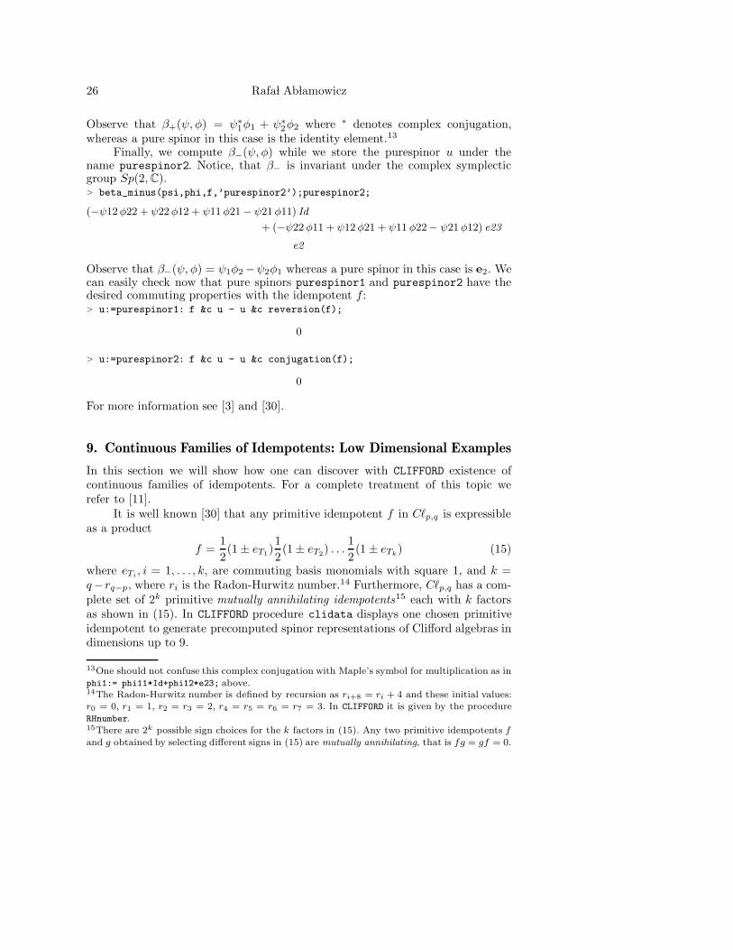
Observe that β+(ψ, φ) = ψ∗1φ1 + ψ∗
2φ2 where ∗ denotes complex conjugation,whereas a pure spinor in this case is the identity element.13
Finally, we compute β−(ψ, φ) while we store the purespinor u under thename purespinor2. Notice, that β− is invariant under the complex symplecticgroup Sp(2,C).> beta_minus(psi,phi,f,’purespinor2’);purespinor2;
(−ψ12φ22 + ψ22φ12 + ψ11φ21 − ψ21φ11) Id
+ (−ψ22φ11 + ψ12φ21 + ψ11 φ22 − ψ21φ12) e23
e2
Observe that β−(ψ, φ) = ψ1φ2 −ψ2φ1 whereas a pure spinor in this case is e2. Wecan easily check now that pure spinors purespinor1 and purespinor2 have thedesired commuting properties with the idempotent f :> u:=purespinor1: f &c u - u &c reversion(f);
0
> u:=purespinor2: f &c u - u &c conjugation(f);
0
For more information see [3] and [30].
9. Continuous Families of Idempotents: Low Dimensional Examples
In this section we will show how one can discover with CLIFFORD existence ofcontinuous families of idempotents. For a complete treatment of this topic werefer to [11].
It is well known [30] that any primitive idempotent f in C`p,q is expressibleas a product
f =1
2(1 ± eT1)
1
2(1 ± eT2) . . .
1
2(1 ± eTk
) (15)
where eTi, i = 1, . . . , k, are commuting basis monomials with square 1, and k =
q− rq−p, where ri is the Radon-Hurwitz number.14 Furthermore, C`p,q has a com-plete set of 2k primitive mutually annihilating idempotents15 each with k factorsas shown in (15). In CLIFFORD procedure clidata displays one chosen primitiveidempotent to generate precomputed spinor representations of Clifford algebras indimensions up to 9.
13One should not confuse this complex conjugation with Maple’s symbol for multiplication as in
phi1:= phi11*Id+phi12*e23; above.14The Radon-Hurwitz number is defined by recursion as ri+8 = ri + 4 and these initial values:r0 = 0, r1 = 1, r2 = r3 = 2, r4 = r5 = r6 = r7 = 3. In CLIFFORD it is given by the procedure
RHnumber.15There are 2k possible sign choices for the k factors in (15). Any two primitive idempotents f
and g obtained by selecting different signs in (15) are mutually annihilating, that is fg = gf = 0.

Computations with Clifford and Grassmann Algebras 27
We will show how to find continuous families of idempotents in a Clifford al-gebra C`(Q) by finding a general solution to the equation f2 = f with a procedureclisolve. As low dimensional examples, we will use C`2,0, C`1,1 and C`3,0.
Example 4. Families of idempotents in C`2,0 (see also [43]) can be discovered asfollows.> dim_V:=2:B:=diag(1,1):bas:=cbasis(dim_V):clidata();
[real , 2, simple,Id
2+
e1
2, [Id , e2 ], [Id], [Id, e2 ]]
As shown above, a standard primitive idempotent inC`2,0 is f1 = 12+ 1
2e1. We
will look, however, for the most general element f in C`2,0 that satisfies f2 = f.> f:=add(x[i]*bas[i],i=1..2^dim_V);
f := x1 Id + x2 e1 + x3 e2 + x4 e12
There are four real solutions:> sol:=map(allvalues,clisolve(cmul(f,f)-f,f)):sol_real:=remove(has,sol,I);
sol real := [0, Id ,Id
2+
1
2
√1 + 4x4
2 e2 + x4 e12 ,Id
2− 1
2
√1 + 4x4
2 e2 + x4 e12 ,
Id
2+
1
2
√1 − 4x3
2 + 4x42 e1 + x3 e2 + x4 e12 ,
Id
2− 1
2
√1 − 4x3
2 + 4x42 e1 + x3 e2 + x4 e12 ]
We verify that each solution is an idempotent (of course, 0 and Id are the trivialones):> map(x -> is(simplify(cmul(x,x)=x)),sol_real);
[true, true, true, true, true, true]
Observe that all nontrivial idempotents found above are ungraded, i.e., theyare neither odd nor even. If we set x4 = x3 = 0 in the above two idempotents thatcontain
√1 − 4 x3
2 + 4 x42, we recover the default mutually annihilating primitive
pair. However,
1
2± 1
2
√
1 + 4 x42 − 4 x3
2 e1 + x3 e2 + x4 e1 ∧ e2 (16)
gives a two-parameter family of idempotents inC`2,0 as long as 1+4 x42−4 x3
2 ≥ 0.The classical (discrete) idempotents occupy the center (0, 0) of that parameterizedregion in the real x3x4-plane. It can be easily checked that the above two idempo-tents, in general, do not add up to 1 and do not annihilate each other unless bothparameters are zero.
Example 5. Let’s now change the signature from (2, 0) to (1, 1) and repeat theabove computations in the Clifford algebra C`1,1 of neutral signature.> dim_V:=2:B:=diag(1,-1):bas:=cbasis(dim_V):clidata();
[real , 2, simple,Id
2+
e12
2, [Id, e1 ], [Id ], [Id , e1 ]]

28 Rafa l Ab lamowicz
> f:=add(x[i]*bas[i],i=1..2^dim_V);
f := x1 Id + x2 e1 + x3 e2 + x4 e12
> sol:=map(allvalues,clisolve(cmul(f,f)-f,f)):sol_real:=remove(has,sol,I);
sol real := [0, Id ,Id
2+
1
2
√1 − 4x4
2 e2 + x4 e12 ,Id
2− 1
2
√1 − 4x4
2 e2 + x4 e12 ,
Id
2+
1
2
√1 + 4x3
2 − 4x42 e1 + x3 e2 + x4 e12 ,
Id
2− 1
2
√1 + 4x3
2 − 4x42 e1 + x3 e2 + x4 e12 ]
> map(x -> is(simplify(cmul(x,x)=x)),sol_real);
[true, true, true, true, true, true]
Thus, like in the Euclidean case, we find that
1
2± 1
2
√
1 + 4 x32 − 4 x4
2 e1 + x3 e2 + x4 e1 ∧ e2 (17)
gives a two parameter family of idempotents provided 1 + 4 x32 − 4 x4
2 ≥ 0. Likein the Euclidean case we find that the idempotents in the pair (17) do not addup to 1 and do not mutually annihilate unless x3 = x4 = 0. In that case we findgraded idempotents 1
2± 1
2e1 ∧ e2.
In the anti-Euclidean signature (0, 2) we only find, as expected, trivial idem-potents in C`0,2 ' H. In higher dimensions, for example in C`3,0, one also findsfamilies parameterized by more than two parameters.
10. Vahlen Matrices
For the background material on Vahlen matrices and conformal transformations,see [15, 31, 33,34,38]. Procedure isVahlenmatrix determines if a given 2 × 2 Clif-ford matrix V ∈ Mat(2, C`(Q)) is a Vahlen matrix and it returns true or false
accordingly. Any matrix with entries in a Clifford algebra is of ‘type/climatrix‘.A Vahlen matrix is a 2×2 matrix V =
(
a bc d
)
with entries in a Clifford algebraC`p,q such that the following conditions are met:
1. a, b, c, d are products of 1-vectors,2. The pseudo-determinant16 of V computed as ad− bc equals +1 or −1,3. ab, bd, dc, and ca are all 1-vectors.17
Condition (i) above implies that a, b, c, and d are elements of the Lipschitzgroup Lp,q of C`p,q. Recall [35] that this group is defined as follows:
Lp,q = {s ∈ C`p,q | xxs−1 ∈ Rp,q,x ∈ R
p,q}.
16In CLIFFORD it is computed with a procedure pseudodet.17Here ˜ denotes the reversion anti-automorphism in C`p,q . In CLIFFORD it is the reversion
operation.

Computations with Clifford and Grassmann Algebras 29
Procedure isproduct is used to determine whether this condition is met. Recallthat in dimensions n ≥ 3 sense preserving conformal mappings are restrictions ofthe Mobius transformations and are compositions of rotations, translations, dila-tions and transversions (called also special conformal transformations). A Mobiustransformation in R
p,q can be written in the form
x → ax + b
cx + d(18)
where x is a 1-vector that belongs to Rp,q , a, b, c, d belong to C`p,q, and the prod-ucts and the inverse are taken in C`p,q. This transformation may be representedby the Vahlen matrix V defined above. Rotations, translations, dilations, andtransversions will then be represented as follows:
• Rotations: x → axa−1 where a belongs to Spin+(p, q), the identity compo-
nent of Spin(p, q), and V =
(
a 00 a
)
,
• Translations: x → x + b where b ∈ Rp,q and V =
(
1 b
0 1
)
,
• Dilations: x → sx where s > 0 and V =
(√s 0
0 1√s
)
,
• Transversions: x → (x + x2c)
(1 + 2x · c + x2c2)where c ∈ Rp,q, x·c is the dot product
in Rp,q and V =
(
1 0c 1
)
.
Let’s consider a few simple examples in the signature (3, 1). Our goal is to seehow CLIFFORD manipulates with Clifford matrices. At the same time we will verifysome results from [38]. We begin with a Vahlen matrix R that gives a rotation:> B:=linalg[diag](1,1,1,-1); #bilinear form for the Minkowski space
B :=
2
6
6
6
6
6
6
4
1 0 0 0
0 1 0 0
0 0 1 0
0 0 0 −1
3
7
7
7
7
7
7
5
> a:=e1we2; #an element of grade 2 in Spin+(3,1)> R:=linalg[matrix](2,2,[a,0,0,a]); #Vahlen matrix that gives a rotation> ’isVahlenmatrix(R)’=isVahlenmatrix(R);
a := e12 , R :=
2
4
e12 0
0 e12
3
5
′isVahlenmatrix (R)′ = true

30 Rafa l Ab lamowicz
Next, we consider a Vahlen matrix T that gives a translation:> b:=e1+2*e3; #vector in R^(3,1)> T:=linalg[matrix](2,2,[1,b,0,1]);> ’isVahlenmatrix(T)’=isVahlenmatrix(T);
b := e1 + 2 e3 , T :=
2
4
1 e1 + 2 e3
0 1
3
5
′isVahlenmatrix(T )′ = true
A Vahlen matrix Dil that gives a dilation transformation:> delta:=1/4: #a positive parameter> Dil:=linalg[matrix](2,2,[sqrt(delta),0,0,1/sqrt(delta)]);> ’isVahlenmatrix(Dil)’=isVahlenmatrix(Dil);
Dil :=
2
6
4
1
20
0 2
3
7
5
′isVahlenmatrix(Dil)′ = true
Finally, a Vahlen matrix Tv that gives a transversion transformation:> c:=2*e1-e3; #a vector in R^(3,1)> Tv:=linalg[matrix](2,2,[1,0,c,1]);> ’isVahlenmatrix(Tv)’=isVahlenmatrix(Tv);
c := 2 e1 − e3 , Tv :=
2
4
1 0
2 e1 − e3 1
3
5
′isVahlenmatrix (Tv)′ = true
If we now take a product of these four matrices above,18 we will obtain an elementconf of the conformal group in R3,1:> conf:=R &cm T &cm Dil &cm Tv;
conf :=
2
6
4
e12
2+ 10 e23 4 e123 − 2 e2
−2 e123 − 4 e2 2 e12
3
7
5
Since in the product above each matrix appeared exactly once, the diagonal entriesof conf must be invertible. We find the inverses of each element with cinv:> cinv(conf[1,1]); #inverse of conf[1,1]
−2 e12
401− 40 e23
401
18&cm denotes a matrix multiplication in CLIFFORDwith the Clifford product applied to the matrix
entries.

Computations with Clifford and Grassmann Algebras 31
> cinv(conf[2,2]); #inverse of conf[2,2]
−e12
2
However, there are elements in the conformal group of R3,1 whose Vahlen matricesdo not have invertible elements at all. The following example of such matrix isdue to Johannes Maks. [38] Matrix W defined below represents an element in theidentity component of the conformal group of R
3,1:> W:=evalm((1/2)*linalg[matrix](2,2,[1-e14,-e1+e4,e1+e4,1+e14]));
W :=
2
6
6
4
1
2− e14
2−e1
2+
e4
2
e1
2+
e4
2
1
2+
e14
2
3
7
7
5
Notice that the diagonal elements of W are non-trivial idempotents in C`3,1 henceas such they are not invertible:> type(W[1,1],idempotent); #element (1,1) of W is an idempotent
true
> type(W[2,2],idempotent); #element (2,2) of W is an idempotent
true
Notice also that the off-diagonal elements of W are isotropic vectors in R3,1, hence
they are also non-invertible. In C`3,1 such vectors have zero squares:> cmul(W[1,2],W[1,2]),cmul(W[2,1],W[2,1]);
0, 0
Let’s now verify that matrix W defined above is a Vahlen matrix:> ’isVahlenmatrix(W)’=isVahlenmatrix(W);
true
However, matrix W represents an element of the identity component of the con-formal group in R3,1 since its pseudo-determinant is 1, and since it can be writtenas a product of a transversion, a translation, and a transversion. Thus, in an-other words, W is not a product of just one rotation, one translation, one dilation,
and/or one transversion:> Tv:=linalg[matrix](2,2,[1,0,(e1+e4)/2,1]);
Tv :=
2
4
1 0e4
2+
e1
21
3
5
> T:=linalg[matrix](2,2,[1,(-e1+e4)/2,0,1]);
T :=
2
6
4
1e4
2− e1
2
0 1
3
7
5
32 Rafa l Ab lamowicz
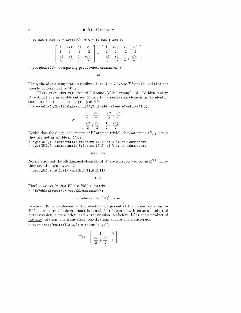
> Tv &cm T &cm Tv = evalm(W); # W = Tv &cm T &cm Tv
2
6
6
4
1
2− e14
2
e4
2− e1
2
e4
2+
e1
2
1
2+
e14
2
3
7
7
5
=
2
6
6
4
1
2− e14
2
e4
2− e1
2
e4
2+
e1
2
1
2+
e14
2
3
7
7
5
> pseudodet(W); #computing pseudo-determinant of W
Id
Thus, the above computation confirms that W = Tv&cmT &cmTv and that thepseudo-determinant of W is 1.
There is another variation of Johannes Maks’ example of a Vahlen matrixW without any invertible entries. Matrix W represents an element in the identitycomponent of the conformal group of R3,1.> W:=evalm((1/2)*linalg[matrix](2,2,[1-e24,-e2+e4,e2+e4,1+e24]));
W :=
2
6
6
4
1
2− e24
2−e2
2+
e4
2
e2
2+
e4
2
1
2+
e24
2
3
7
7
5
Notice that the diagonal elements of W are non-trivial idempotents in C`3,1, hencethey are not invertible in C`3,1:> type(W[1,1],idempotent); #element (1,1) of W is an idempotent> type(W[2,2],idempotent); #element (2,2) of W is an idempotent
true , true
Notice also that the off-diagonal elements of W are isotropic vectors in R3,1, hencethey are also non-invertible:> cmul(W[1,2],W[1,2]),cmul(W[2,1],W[2,1]);
0, 0
Finally, we verify that W is a Vahlen matrix:> ’isVahlenmatrix(W)’=isVahlenmatrix(W);
′isVahlenmatrix (W)′ = true
However, W is an element of the identity component of the conformal group inR3,1 since its pseudo-determinant is 1, and since it can be written as a product ofa transversion, a translation, and a transversion. As before, W is not a product ofjust one rotation, one translation, one dilation, and/or one transversion:
> Tv:=linalg[matrix](2,2,[1,0,(e2+e4)/2,1]);
Tv :=
2
4
1 0e4
2+
e2
21
3
5

Computations with Clifford and Grassmann Algebras 33
> T:=linalg[matrix](2,2,[1,(-e2+e4)/2,0,1]);
T :=
2
6
4
1e4
2− e2
2
0 1
3
7
5
> Tv &cm T &cm Tv = evalm(W); #W = Tv &cm T &cm Tv
2
6
6
4
1
2− e24
2
e4
2− e2
2
e4
2+
e2
2
1
2+
e24
2
3
7
7
5
=
2
6
6
4
1
2− e24
2
e4
2− e2
2
e4
2+
e2
2
1
2+
e24
2
3
7
7
5
> pseudodet(W); #computing pseudo-determinant of W
Id
Thus, the above computation again confirms that W = Tv&cmT &cmTv andthat the pseudo-determinant of W is 1.
11. Singular Value Decomposition and Clifford Algebra
In this section we will show how the Singular Value Decomposition (SVD) of amatrix can be translated into the Clifford algebra language. For the backgroundinformation on SVD we refer to [42]. There are many uses of SVD such as in imageprocessing, description of the so called principal gains in a multivariable system[37], or in an automated data indexing known as Latent Semantic Indexing (orLSI). LSI presents a very interesting and useful technique in information retrievalmodels and it is based on the SVD. [19] While in these practical cases computationsare done numerically, it may be of interest to ask whether SVD of a matrix canbe performed in the framework of Clifford algebras. Likewise, whether SVD of aClifford number can be found without using matrices. That is, if any new insights,theoretical or otherwise, into such decomposition could be gained when stated inthe Clifford algebra language.
We will explore a well-known fact that when p − q 6= 1 mod 4, the Cliffordalgebra C`p,q is a simple algebra of dimension 2n, n = p + q, isomorphic to a
full matrix algebra Mat(2k,K) of 2k × 2k matrices19 with entries in the divisionring K. The ring K is a subalgebra of C`p,q isomorphic to R, C, or H depending onthe signature (p, q) and the dimension n (see [3]). Thus, any operation performedon a matrix A ∈ Mat(2k,K) can be expressed as an operation on the uniquelycorresponding to it element p in C`p,q. The choice of the signature (p, q) dependson the size of A and the division ring K. Of course, for computational reasons oneshould find the smallest Clifford algebra C`p,q such that the given matrix A can be
19The value k is determined by the formula k = q−rq−p, where ri is the Radon-Hurwitz number.The Radon-Hurwitz number is defined by a recursion as ri+8 = ri + 4 and these initial values:
r0 = 0, r1 = 1, r2 = r3 = 2, r4 = r5 = r6 = r7 = 3.

34 Rafa l Ab lamowicz
embedded into Mat(2k,K)ϕ' C`p,q. In the following we will use the same approach
as in [2] where a technique for matrix exponentiation based on the isomorphism ϕ
was presented. In particular, we will use a faithful spinor representation of C`p,q ina minimal left ideal S = C`p,qf generated by a primitive idempotent f. Symboliccomputations of such representations with CLIFFORD were shown in [3].
Following [42], let A be an m× n real matrix of rank r. Then the SVD of Ais defined a factorization of A into a product of three matrices U,Σ, V −1 where Uand V are orthogonal matrices m×m and n × n respectively, and Σ is a m × n
matrix containing singular values of A on its “diagonal”.
A = UΣV −1, UTU = I, V TV = I. (19)
The matrices V = [v1|v2| . . . |vn] and U = [u1|u2| . . . |um] contain orthonormalbases for all four fundamental spaces of A. Namely, the first r columns v1, v2, . . . , vr
of V provide a basis for the row space R(AT ) while the remaining n−r columns of Vprovide a basis for the null space N (A). Likewise, the first r columns u1, u2, . . . , ur
of U provide a basis for the column space C(A) while the remaining m−r columnsof U provide a basis for the left-null space N (AT ). Vectors vi are the normalizedeigenvectors of ATA while vectors ui are the normalized eigenvectors of AAT . Fori = 1, . . . , r, these vectors can be chosen to be related via the positive singularvalues σi of A which are just the square roots of the eigenvalues of ATA (or ofAAT .) Namely,
Avi = σiui, i = 1, . . . , r. (20)
It is a little tricky to make sure that the above relation is satisfied: this is becausethe choice of vectors ui is independent of the choice of vectors vi. However, it is al-ways possible to do so as we will see below (see also [42]). In order to complete thepicture, the orthonormal set {v1, . . . , vr} needs to be completed to a full orthonor-mal basis for Rn while {u1, . . . , ur} needs to be completed to a full orthonormalbasis for Rm. Since the additional vectors are being annihilated by A and AT re-spectively, that is, they are eigenvectors of A and AT (or of ATA and AAT ) thatcorrespond to the eigenvalue 0, care has to be exercised when finding them. Forexample, while the eigenvectors of the symmetric matrix AAT are automaticallyorthogonal provided they correspond to different eigenvalues, eigenvectors of AAT
that correspond to the 0 eigenvalue don’t need to be orthogonal: in this case theGram-Schmidt orthogonalization process is used to complete the two sets.
11.1. SVD of a 2 × 2 matrix of rank 2
In this section we present a simple example of SVD of a 2×2 real matrix of rank 2.The purpose of this example is just to show step by step how finding the SVD ofa matrix can be done in the Clifford algebra language. Reader is encouraged toperform these computations with CLIFFORD and an additional package asvd.20
> A:=matrix(2,2,[2,3,1,2]); #defining A
20Package asvd contains the following procedures used in the text: phi that provides an iso-
morphism between a matrix algebra and a Clifford algebra; radsimplify that simplifies radicalexpressions in matrices and vectors; assignL that writes an output from a Maple procedure
eigenvects in a suitable form: it sorts eigenvectors according to the corresponding eigenvalues

Computations with Clifford and Grassmann Algebras 35
A :=
2
4
2 3
1 2
3
5
Since A ∈ Mat(2,R), we need to find (p, q) such that C`p,q
ϕ' Mat(2,R). Procedureall sigs built into CLIFFORD displays two possible choices for the signature (p, q)such that p+ q = 2, K ' R and C`p,q is a simple algebra:> all_sigs(2..2,real,simple);
[[1, 1], [2, 0]]
Thus, we can pick either C`1,1 or C`2,0. Our choice is C`2,0. We define B as the2×2 identity matrix and use CLIFFORD’s procedure clidata to display informationabout C`2,0.> dim:=2:B:=diag(1,1):eval(makealiases(dim)):data:=clidata();
data := [real , 2, simple,1
2Id +
1
2e1 , [Id, e2 ], [Id ], [Id , e2 ]]
The above output means that C`2,0 is a simple algebra isomorphic to Mat(2,R);that the element 1
2+1
2e1 displayed by Maple as 1
2Id+1
2e1 is a primitive idempotent;
that the list [Id , e2 ] shown as the fifth entry displays generators of a minimalleft-ideal C`2,0f considered as vector space over R; that the division ring K =fC`2,0f = 〈Id〉R ' R; and that the last list [Id , e2 ] gives generators of C`2,0f
over K, and, since K ' R, it is the same as the fifth entry.21In the following,we define a Grassmann basis in C`2,0, assign the primitive idempotent to f, andgenerate a spinor basis in C`2,0f.> clibas:=cbasis(dim); #ordered basis in Cl(2,0)
clibas := [Id, e1 , e2 , e12 ]
> f:=data[4]:#a primitive idempotent in Cl(2,0)> SBgens:=data[5]:#generators for a real basis in S> FBgens:=data[6]:#generators for the division ring KSBgens contains generators for a K-basis for S = C`2,0f = 〈f, e2f〉. Since inthe signature (2, 0) we have K ' R, S ' R2, and C`2,0 ' Mat(2,R), the outputfrom the procedure spinorKbasis shown below has two basis elements and theirgenerators modulo f :> Kbasis:=spinorKbasis(SBgens,f,FBgens,’left’);
Kbasis := [[1
2Id +
1
2e1 ,
1
2e2 − 1
2e12 ], [Id , e2 ], left]
Thus, the real spinor basis in S consists of the following two polynomials:> for i to nops(Kbasis[1]) do f.i:=Kbasis[1][i] od;
f1 :=1
2Id +
1
2e1 , f2 :=
1
2e2 − 1
2e12 .
and it uses the Gram-Schmidt orthogonalization process, if necessary, to return a complete listof orthogonal eigenvectors; makediag makes a “diagonal” Σ matrix consisting of singular values.21For more information see [3] and help pages in CLIFFORD.

36 Rafa l Ab lamowicz
We are in position now to compute matrices M1,M2,M3,M4 representing each ofthe four basis elements {1, e1, e2, e12} of C`2,0 in the basis {f1, f2}.22
> for i to nops(clibas) do M[i]:=subs(Id=1,matKrepr(clibas[i])) end do:
We will use a new procedure phi which realizes the isomorphism ϕ from Mat(2,R)to C`2,0. This way we can find the image p = ϕ(A) in C`2,0 of any real 2 × 2matrix A. Knowing image ϕ(Mi) of each matrix Mi, i = 1, . . . , 4, in terms of someClifford polynomial in C`2,0 we can easily find p = ϕ(A) as follows:23
> p:=phi(A,M); #finding image of A in Cl(2,0)
p := 2 Id + 2 e2 + e12
> pT:=phi(t(A),M); #finding image of t(A) in Cl(2,0)
pT := 2 Id + 2 e2 − e12
Next, we compute a symmetric matrix ATA (denoted in Maple as ATA),its characteristic polynomial, eigenvalues, and its orthonormal eigenvectors v1, v2.Vectors v1 and v2 will become columns of an orthogonal matrix V needed for theSVD of A:> ATA:=evalm(t(A) &* A); #finding matrix ATA
ATA :=
2
4
5 8
8 13
3
5
> pTp:=phi(ATA,M); #finding image of ATA in Cl(2,0)
pTp := 9 Id − 4 e1 + 8 e2
which is the same as> ’pTp’=cmul(pT,p);
pTp = 9 Id − 4 e1 + 8 e2
The minimal polynomial of ATA, whose image in C`2,0 is called pTp, is computedwith climinpoly:> climinpoly(pTp);
x2 − 18 x+ 1
and it is the same as the characteristic polynomial of ATA:> pol:=charpoly(ATA,x);#characteristic polynomial of ATA
pol := x2 − 18 x+ 1
22Since a similar computation was done in [2, 3], we won’t display the matrices.23From now on, we use Maple’s alias(t = transpose), that is, t(A) denotes matrix transpo-sition in Maple. The second argument to the procedure phi is a table M containing matrices
M1, M2, M3, M4 as its entries.
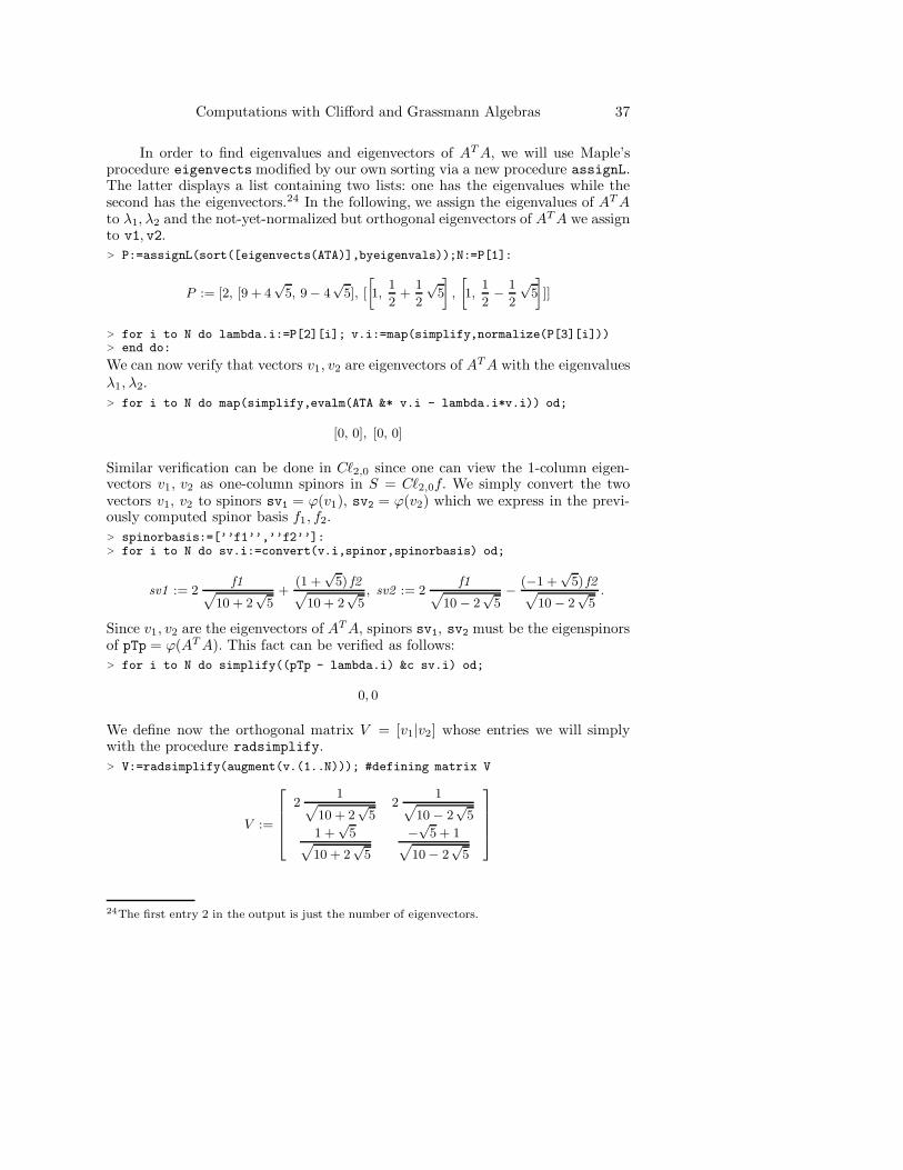
Computations with Clifford and Grassmann Algebras 37
In order to find eigenvalues and eigenvectors of ATA, we will use Maple’sprocedure eigenvects modified by our own sorting via a new procedure assignL.The latter displays a list containing two lists: one has the eigenvalues while thesecond has the eigenvectors.24 In the following, we assign the eigenvalues of ATAto λ1, λ2 and the not-yet-normalized but orthogonal eigenvectors of ATA we assignto v1, v2.
> P:=assignL(sort([eigenvects(ATA)],byeigenvals));N:=P[1]:
P := [2, [9 + 4√
5, 9 − 4√
5], [
»
1,1
2+
1
2
√5
–
,
»
1,1
2− 1
2
√5
–
]]
> for i to N do lambda.i:=P[2][i]; v.i:=map(simplify,normalize(P[3][i]))> end do:
We can now verify that vectors v1, v2 are eigenvectors of ATA with the eigenvaluesλ1, λ2.
> for i to N do map(simplify,evalm(ATA &* v.i - lambda.i*v.i)) od;
[0, 0], [0, 0]
Similar verification can be done in C`2,0 since one can view the 1-column eigen-vectors v1, v2 as one-column spinors in S = C`2,0f. We simply convert the twovectors v1, v2 to spinors sv1 = ϕ(v1), sv2 = ϕ(v2) which we express in the previ-ously computed spinor basis f1, f2.> spinorbasis:=[’’f1’’,’’f2’’]:> for i to N do sv.i:=convert(v.i,spinor,spinorbasis) od;
sv1 := 2f1
p
10 + 2√
5+
(1 +√
5) f2p
10 + 2√
5, sv2 := 2
f1p
10 − 2√
5− (−1 +
√5) f2
p
10 − 2√
5.
Since v1, v2 are the eigenvectors of ATA, spinors sv1, sv2 must be the eigenspinorsof pTp = ϕ(ATA). This fact can be verified as follows:> for i to N do simplify((pTp - lambda.i) &c sv.i) od;
0, 0
We define now the orthogonal matrix V = [v1|v2] whose entries we will simplywith the procedure radsimplify.
> V:=radsimplify(augment(v.(1..N))); #defining matrix V
V :=
2
6
6
6
4
21
p
10 + 2√
52
1p
10 − 2√
5
1 +√
5p
10 + 2√
5
−√
5 + 1p
10 − 2√
5
3
7
7
7
5
24The first entry 2 in the output is just the number of eigenvectors.

38 Rafa l Ab lamowicz
Since later we will need images of V and V T under ϕ in C`2,0, we compute themnow and store them under the variables pV and pVt respectively.> pV:=phi(V,M); #finding image of V in Cl(2,0)> pVt:=phi(t(V),M): #finding image of t(V) in Cl(2,0)
pV :=
(− 1
20%1
√5 − 1
40%2
√5 +
1
8%2) Id + (
1
20%1
√5 − 1
40%2
√5 +
1
8%2) e1
+ (1
20%2
√5 +
1
40%1
√5 +
1
8%1) e2 + (− 1
20%2
√5 +
1
40%1
√5 +
1
8%1) e12
%1 :=p
10 − 2√
5
%2 :=p
10 + 2√
5The fact that V is orthogonal can be easily verified in the matrix language; inC`2,0 it can be done as follows:> simplify(cmul(pVt,pV));
Id
We repeat the above steps and apply them to AAT . In the process, we will find itseigenvectors u1, u2. We must make sure that Avi = σiui where σi =
√λi, i = 1, 2.
This will require extra checking and possibly redefining of the u’s.> AAT:=evalm(A &* transpose(A)); #computing AAT
AAT :=
2
4
13 8
8 5
3
5
The image of AAT under ϕ in C`2,0 we denote as ppT.> ppT:=phi(AAT,M); #finding image of AAT in Cl(2,0)
ppT := 9 Id + 4 e1 + 8 e2
In this case, the minimal polynomial of ppT and the characteristic polynomial ofAAT are, of course, the same.> pol2:=charpoly(AAT,lambda); #characteristic polynomial of AAT
pol2 := λ2 − 18λ+ 1
> ’ppT’=climinpoly(ppT);
ppT = x2 − 18 x+ 1
Since matrices ATA and AAT have the same characteristic polynomials, theireigenvalues λ1, λ2 will be the same. We define therefore the singular values σ1 andσ2 of A as the square roots of λ1 and λ2.> for i to N do sigma.i:=sqrt(lambda.i) od;
σ1 :=√
5 + 2, σ2 :=√
5 − 2
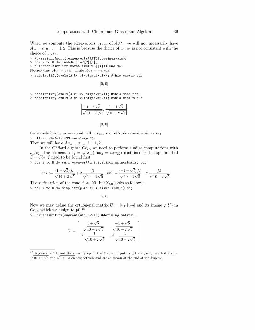
Computations with Clifford and Grassmann Algebras 39
When we compute the eigenvectors u1, u2 of AAT , we will not necessarily haveAvi = σiui, i = 1, 2. This is because the choice of u1, u2 is not consistent with thechoice of v1, v2.> P:=assignL(sort([eigenvects(AAT)],byeigenvals)):> for i to N do lambda.i:=P[2][i];> u.i:=map(simplify,normalize(P[3][i])) end do:
Notice that Av1 = σ1u1 while Av2 = −σ2u2:> radsimplify(evalm(A &* v1-sigma1*u1)); #this checks out
[0, 0]
> radsimplify(evalm(A &* v2-sigma2*u2)); #this does not> radsimplify(evalm(A &* v2+sigma2*u2)); #this checks out
"
14 − 6√
5p
10 − 2√
5,
8 − 4√
5p
10 − 2√
5
#
[0, 0]
Let’s re-define u2 as −u2 and call it u22, and let’s also rename u1 as u11:> u11:=evalm(u1):u22:=evalm(-u2):
Then we will have Avii = σuii, i = 1, 2.In the Clifford algebra C`2,0 we need to perform similar computations with
v1, v2. The elements su1 = ϕ(u11), su2 = ϕ(u22) contained in the spinor idealS = C`2,0f need to be found first.> for i to N do su.i:=convert(u.i.i,spinor,spinorbasis) od;
su1 :=(1 +
√5) f1
p
10 + 2√
5+ 2
f2p
10 + 2√
5, su2 :=
(−1 +√
5) f1p
10 − 2√
5− 2
f2p
10 − 2√
5.
The verification of the condition (20) in C`2,0 looks as follows:> for i to N do simplify(p &c sv.i-sigma.i*su.i) od;
0, 0
Now we may define the orthogonal matrix U = [u11|u22] and its image ϕ(U) inC`2,0 which we assign to pU:25
> U:=radsimplify(augment(u11,u22)); #defining matrix U
U :=
2
6
6
6
4
1 +√
5p
10 + 2√
5
−1 +√
5p
10 − 2√
5
21
p
10 + 2√
5−2
1p
10 − 2√
5
3
7
7
7
5
25Expressions %1 and %2 showing up in the Maple output for pU are just place holders forp
10 + 2√
5 andp
10 − 2√
5 respectively and are as shown at the end of the display.

40 Rafa l Ab lamowicz
> pU:=phi(U,M);#finding image of U in Cl(2,0)> pUt:=phi(t(U),M):#finding image of t(U) in Cl(2,0)
pU := (1
20%1
√5 − 1
8%2 − 1
40%2
√5) Id + (
1
20%1
√5 +
1
8%2 +
1
40%2
√5) e1
+ (1
20%2
√5 +
1
8%1 − 1
40%1
√5) e2 + (
1
20%2
√5 − 1
8%1 +
1
40%1
√5) e12
%1 :=p
10 + 2√
5
%2 :=p
10 − 2√
5The fact that U is an orthogonal matrix can be easily now checked both in thematrix language and in the Clifford language:> radsimplify(evalm(t(U) &* U));#U is an orthogonal matrix
2
4
1 0
0 1
3
5
> simplify(pUt &c pU);
Id
Finally, we define matrix Σ using a procedure makediag. Recall from [42] thatΣ has the same dimensions as the original matrix A and that ΣT Σ,ΣΣT are thediagonal forms of ATA and AAT respectively. In this example matrices ΣT Σ andΣΣT are the same since Σ is a square diagonal matrix. Normally these matricesare different although their nonzero “diagonal” entries are the same. Therefore wehave
ATA = VΣT ΣV T , AAT = UΣΣTUT , Σ =
[
σ1 00 σ2
]
,
ΣT Σ = ΣΣT =
[
σ21 0
0 σ22
]
.
(21)
Matrices Σ, ΣT Σ and ΣΣT we assign to Maple variables Sigma, STS and SST re-spectively:> Sigma:=makediag(m,n,[seq(sigma.i,i=1..N)]);> STS,SST:=evalm(t(Sigma) &* Sigma),evalm(Sigma &* t(Sigma));
Σ :=
2
4
√5 + 2 0
0√
5 − 2
3
5
STS , SST :=
2
4
(√
5 + 2)2 0
0 (√
5 − 2)2
3
5 ,
2
4
(√
5 + 2)2 0
0 (√
5 − 2)2
3
5
The corresponding images ϕ(Σ), ϕ(ΣT Σ) and ϕ(ΣΣT ) and C`2,0 will be assignedto the Maple variables pSigma, pSTS and pSST respectively:> pSigma,pSTS,pSST:=phi(Sigma,M),phi(STS,M,FBgens),phi(SST,M);
pSigma, pSTS , pSST :=√
5 Id + 2 e1 , 9 Id + 4√
5 e1 , 9 Id + 4√
5 e1

Computations with Clifford and Grassmann Algebras 41
We should be able to verify in C`2,0 the following two factorizations of AAT andATA:
ATA = V ΣT ΣV T (22)
AAT = UΣΣTUT (23)
like this:> evalb(pTp=simplify(pV &c pSTS &c pVt)),> evalb(ppT=simplify(pU &c pSST &c pUt));
true, true
Finally, we check the SVD of A, which is A = UΣV T ,26 in the Clifford algebralanguage:> evalb(p=simplify(pU &c pSigma &c pVt));
true
11.2. Additional comments
In the previous section we have shown that it is possible to translate the ma-trix algebra picture of the Singular Value Decomposition of a matrix A into theClifford algebra language. Although we have not abandoned entirely the linearalgebra formalism in our example, e.g., we have computed the eigenvalues andthe eigenvectors of ATA and AAT , and only then we have found images of theireigenvectors in the spinor space C`2,0f, these computations including solving theeigenvalue problem can be done entirely in the Clifford algebra language. In thefollowing we show how this can be accomplished.
The first comment is that it is also possible to compute the eigenvalues λ1, λ2
and the eigenspinors sv1 = ϕ(v1), sv2 = ϕ(v2) of the Clifford number pTp =ϕ(ATA) directly inC`2,0 using the procedure clisolve capable of solving algebraicequations.> eigenspinor:=x1*f1+x2*f2;> eigeneq:=clicollect(expand(cmul(pTp,eigenspinor)-lambda*eigenspinor));
eigenspinor := x1 (Id
2+
e1
2) + x2 (
e2
2− e12
2)
eigeneq := − (−5 x1 − 8 x2 + λ x1) e1
2− (−5 x1 − 8 x2 + λ x1) Id
2
+(λ x2 − 13 x2 − 8 x1) e12
2− (λ x2 − 13 x2 − 8 x1) e2
2
26The SVD of A is not unique: For example, A = (−U )Σ(−V T ) is another such factorization.

42 Rafa l Ab lamowicz
> sol:=remove(has,map(allvalues,clisolve(eigeneq,[lambda,x1,x2])),> lambda=lambda);
sol := [{λ = 9 + 4√
5, x2 = x2 , x1 =(9 + 4
√5) x2
8− 13 x2
8},
{λ = 9 − 4√
5, x2 = x2 , x1 =(9 − 4
√5) x2
8− 13 x2
8}]
> for i from 1 to nops(sol) do;> lambda||i:=subs(sol[1],lambda);> eigenspinor||i:=clicollect(subs({x1=1,x2=1},subs(sol[1],eigenspinor)));> end do;
λ1 := 9 + 4√
5
eigenspinor1 :=(−1 +
√5) e1
4+
(−1 +√
5) Id
4− e12
2+
e2
2
λ2 := 9 + 4√
5
eigenspinor2 :=(−1 +
√5) e1
4+
(−1 +√
5) Id
4− e12
2+
e2
2
The second comment is that it is possible to realize an anti-automorphismtp : C`(Q) → C`(Q) that acts on homogeneous basis multivectors as follows:
ei1 ∧ ei2 ∧ · · · ∧ ein7→ Qi1i1Qi2i2 · · ·Qinin
(ei1 ∧ ei2 ∧ · · · ∧ ein)˜ (24)
where (ei1∧ei2∧· · ·∧ein)˜= (−1)
n(n−1)2 ei1∧ei2∧· · ·∧ein
is the reversed multivectorwhile Qi1i1 , Qi2i2 , . . . , Qinin
are the diagonal entries of the quadratic form Q (tobe precise, Qii = e2
i , i = 1, . . . , n), extended by linearity to the whole algebra.Then, tp gives the transposition of the corresponding spinor representation.27 Fora thorough treatment of the singular value decomposition for Grassmann andClifford algebras in the Hopf algebraic language see [23].
12. Conclusions
The aim of this note was to present a few examples of computations with Cliffordalgebras where symbolic capabilities of Maple and the CLIFFORD, BIGEBRA pack-ages were utilized. In some, a better understanding of the Clifford algebra structureand its properties, especially of the Clifford algebras C`(B) of an arbitrary bilin-ear form B, was achieved (see also [6]). Gaining a computational proficiency withClifford algebras of a quadratic form notwithstanding, such as their spinor rep-resentations or computation of bilinear forms on spinor spaces, properties of thecontraction, the reversion, the wedge, the dotted wedge, and the Clifford products,all curiously dependent on the antisymmetric form of B have been successfully for-mulated. In others, a discovery of specific elements was accomplished like finding,
27This has been verified by brute force with CLIFFORD in dimensions up to 9 for simple C`p,q andsuch that (p−q) ≡ 0, 1,2 (mod 8). That is, for the Clifford algebras whose spinor representations
are real. A Maple code for a procedure tp is shown in Appendix C.

Computations with Clifford and Grassmann Algebras 43
unexpectedly continuous, families of idempotents or a computation of eigenvaluesand eigenvectors of a Clifford number, or its singular values. In the process, aconnection between a transposition and the reversion in C`(Q) was discovered.
Some other computational and theoretical results facilitated with the pack-ages and already reported include
• Finding generators for Hecke algebras realized as even elements in a Cliffordalgebra of a suitable, non symmetric, bilinear form. [7]
• Finding q-Young idempotents in some Hecke algebras of mixed symmetrythat generate a representation space for these algebras. [7]
• Finding necessary and sufficient condition that a Clifford biconvolution, thatis, a Clifford Hopf gebra for a two-dimensional real space posses an antipode.[25]
• Investigation of Wick normal ordering [21]• Verification of Helmstetter formula [28] that expresses an isomorphism be-
tween two Clifford algebras C`(B) and C`(B′) where the bilinear forms sharethe symmetric part. [4]
• Explicit description of all elements in Pin(3) and Spin(3) in [4]• Description of space singularities of a robotic platform [5, 17]
For a complete discussion of the mathematical capabilities of CLIFFORD andBIGEBRA packages we refer to [9] and [10].
Appendix A. Appendix: Code of cmulNUM
Here is a pseudocode of the recursive procedure cmulNUM.
cmulNUM(a1,a2,B) [a1, a2 - two Grassmann monomials, B - name of bilinear form]beginif nargs <>3 then error ”exactly three arguments are needed” end ifif has(0,map(simplify,[a1,a2])) then return 0 end ifif a2=‘Id‘ then return a1 end ifif a1=‘Id‘ then return a2 end if
L <- indices from a1N <- length of LcoB,nameB <- coefficient of B, B [to handle -B]if N=0 then return coeff(a1,Id)*a2 elif N=1 then
L2 <- list of indices from a2return reorder(simplify(makeclibasmon([L[1],op(L2)])
+add((-1)ˆ(i-1)*coB*nameB[L[1],L2[i]]*makeclibasmon(subs(L2[i]=NULL,L2)),i=1..nops(L2))))
elif N=2 thenx1 <- substring(a1,1..2)x2 <- substring(a1,4..5)p2 <- procname(x2,a2,B)S <- clibilinear(x1,p2,procname,B)return simplify(S-coB*nameB[op(L)]*a2)
end if;

44 Rafa l Ab lamowicz
x <- cat(e,L[-1])p1 <- substring(a1,1..(3*N-4))p2 <- procname(x,a2,B)S <- clibilinear(p1,p2,procname,B)
-add((-1)ˆ(i)*coB*nameB[L[-i],L[-1]]*procname(makeclibasmon(subs(L[-i]=NULL,L[1..-2])),a2,B),i=2..N)
return reorder(simplify(S))end cmulNUM
Appendix B. Appendix: Code of cmulRS
Here is a pseudocode of the procedure cmulRS based on the combinatorial processof Rota-Stein:
cmulRS(x,y,B) [x, y two Grassmann monomials, B - bilinear form]begin
lstx <- list of indices from xlsty <- list of indices from yNX <- length of lstxNY <- length of lstyfunx <- function maps integers 1..NX onto elements of lstx keeping their orderfuny <- function maps integers 1..NY onto elements of lsty keeping their order
(this is to calculate with arbitrary indices and to compute necessary signs)psetx <- power set of 1..NX (actually a list in a certain order)
(the i-th and (2ˆNX+1-i)-th element are disjoint adding up to the set {1..NX})psety <- power set of 1..NY (actually a list in a certain order)
(the i-th and (2ˆNY+1-i)-th element are disjoint adding up to the set {1..NY})(for faster computation we sort this power sets by grade)(we compute the sign for any term in the power set)
psetx <- sort psetx by gradepsety <- sort psety by gradepSgnx <- sum (i in psetx) (-1)ˆsum (j in psetx[i]) (psetx[i][j]-j)pSgny <- sum (i in psety) (-1)ˆsum (j in psety[i]) (psety[i][j]-j)(we need a subroutine for cup tangle computing the bilinear form cup(x,y,B))begin cupif |x| <> |y| then return 0 end ifif |x| = 0 then return 1 end ifif |x| = 1 then return B[x[1],y[1]] end ifreturn sum (j in 1..|x|)(-1)ˆ(j-1)*B(x[1],y[j])*cup(x[2..-1],y/y[j],B)
end cup(now we compute the double sum, to gain efficiency we do this grade wise)(note that there are r over NX r-vectors in psetx, analogously for psety)max grade - |lstx <- convert_to_set union lsty <- convert_to_set|
res <- 0, pos1 <- 0
for j from 0 to NX (iterate over all j-vectors of psetx)begin
F1 <- N1!/((N1-j)!*j!) (number of terms (N1 over j))
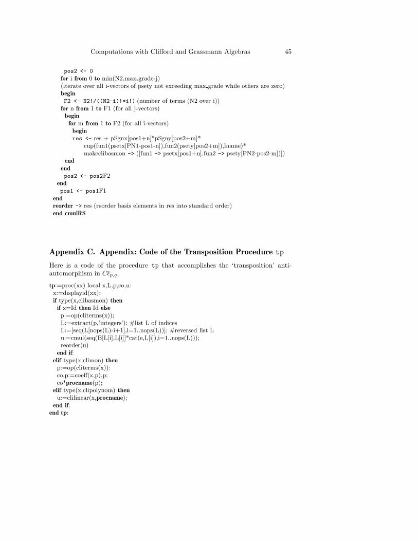
Computations with Clifford and Grassmann Algebras 45
pos2 <- 0
for i from 0 to min(N2,max grade-j)(iterate over all i-vectors of psety not exceeding max grade while others are zero)beginF2 <- N2!/((N2-i)!*i!) (number of terms (N2 over i))
for n from 1 to F1 (for all j-vectors)beginfor m from 1 to F2 (for all i-vectors)beginres <- res + pSgnx[pos1+n]*pSgny[pos2+m]*
cup(fun1(psetx[PN1-pos1-n]),fun2(psety[pos2+m]),lname)*makeclibasmon -> ([fun1 -> psetx[pos1+n],fun2 -> psety[PN2-pos2-m])])
endendpos2 <- pos2F2
endpos1 <- pos1F1
endreorder -> res (reorder basis elements in res into standard order)end cmulRS
Appendix C. Appendix: Code of the Transposition Procedure tp
Here is a code of the procedure tp that accomplishes the ‘transposition’ anti-automorphism in C`p,q.
tp:=proc(xx) local x,L,p,co,u:x:=displayid(xx):if type(x,clibasmon) thenif x=Id then Id else
p:=op(cliterms(x));L:=extract(p,’integers’): #list L of indicesL:=[seq(L[nops(L)-i+1],i=1..nops(L))]; #reversed list Lu:=cmul(seq(B[L[i],L[i]]*cat(e,L[i]),i=1..nops(L)));reorder(u)
end if:elif type(x,climon) then
p:=op(cliterms(x)):co,p:=coeff(x,p),p;co*procname(p);
elif type(x,clipolynom) thenu:=clilinear(x,procname);
end if:end tp:

46 Rafa l Ab lamowicz
References
[1] R. Ab lamowicz, Clifford algebra computations with Maple. In Clifford (Geometric)Algebras with Applications in Physics, Mathematics, and Engineering, W. E. Baylis,ed. (Birkhauser, Boston, 1996) 463–502
[2] R. Ab lamowicz, Matrix exponential via Clifford algebras. J. of Nonlinear Math. Phys.,5, 3 (1998) 294–313
[3] R. Ab lamowicz, Spinor Representations of Clifford Algebras: A Symbolic Approach.CPC Thematic Issue - Computer Algebra in Physics Research, Phys. Comm. 115(1998) 510–535
[4] R. Ab lamowicz, Helmstetter formula and rigid motions with CLIFFORD. In Advancesin Geometric Algebra with Applications in Science and Engineering – AutomaticTheorem proving, Computer Vision, Quantum and Neural Computing, and Robotics,E. Bayro-Corrochano and G. Sobczyk, eds., (Birkhauser, Boston, 2001) 512–534
[5] R. Ab lamowicz, J. Anderson and M. Baswell, Clifford algebra space singularities ofinline planar platforms. In Applications of Geometric Algebra in Computer Scienceand Engineering, L. Dorst, ed., Chapter 36 (Birkhauser, Boston, 2002) 463–502
[6] R. Ab lamowicz and B. Fauser, On the Decomposition of Clifford Algebras of ArbitraryBilinear Form. In Clifford Algebras and their Applications in Mathematical Physics,R. Ab lamowicz and B. Fauser, eds. (Birkhauser, Boston, 2000) 341–366
[7] R. Ab lamowicz and B. Fauser, Hecke algebra representations in ideals generated byq-Young Clifford idempotents. In Clifford Algebras and their Applications in Math-ematical Physics, R. Ab lamowicz and B. Fauser, eds., Vol. 1: Algebra and Physics,(Birkhauser, Boston, 2000) 245–268
[8] R. Ab lamowicz and B. Fauser, CLIFFORD and BIGEBRA for Maple,http://math.tntech.edu/rafal/ (2009)
[9] R. Ab lamowicz and B. Fauser, Mathematics of CLIFFORD - A Maple Package forClifford and Grassmann Algebras. Advances in Applied Clifford Algebras, Vol. 15,No. 2 (2005), 157–181
[10] R. Ab lamowicz and B. Fauser, Clifford and Grassmann Hopf algebras via the BIGEBRApackage for Maple. Computer Physics Communications 170 (2005) 115–130
[11] R. Ab lamowicz, B. Fauser, K. Podlaski and J. Rembielinski, Idempotents of Cliffordalgebras. Czech. J. Phys. 53, 11 (2003) 949–955
[12] R. Ab lamowicz and P. Lounesto, On Clifford algebras of a bilinear form with anantisymmetric part. In Clifford Algebras with Numeric and Symbolic Computations,R. Ab lamowicz, P. Lounesto, and J. Parra, eds. (Birkhauser, Boston, 1996) 167–188
[13] R. Ab lamowicz and G. Sobczyk, Software for Clifford (geometric) algebras. Appendixin Lectures on Clifford (Geometric) Algebras and Applications, R. Ab lamowicz andG. Sobczyk, eds. (Birkhauser, Boston, 2004) 189–209
[14] J.L. Anderson, Green’s functions in quantum electrodynamics, Phys. Rev. 171, 94(1954) 703–11
[15] P. Angles, Construction de revetements du groupe conforme d’un espace vectorielmuni d’uni metrique de type (p, q). Ann. Inst. Henri Poincaree XXXIII, 1 (10980)33–51
[16] Axiom Computer Algebra System, http://en.wikipedia.org/wiki/AXIOM (2009)
Computations with Clifford and Grassmann Algebras 47
[17] M. Baswell, Clifford Algebra Space Singularities of a Redundant Variable GeometryTruss Manipulator. M.S. Thesis, Tennessee Technological University, 2000
[18] CoCoA System for computations in commutative algebra,http://cocoa.dima.unige.it/ (2009)
[19] M. Berry and J. Dongarra, Atlanta Organizers Put Mathematics to Work for theMath Sciences Community, SIAM News, Vol. 32, 6 (1999), and references therein.
[20] Ch. Brouder, B. Fauser, A. Frabetti and R. Oeckl, Quantum field theory and Hopfalgebra cohomology [formerly ‘Let’s twist again’]. J. Phys. A: Math. Gen: 37, 22(2004) 5895–5927
[21] B. Fauser, Clifford geometric parameterization of Wick normal-ordering. J. Phys. A:Math. Gen. 34 (2001) 105–115
[22] B. Fauser, A Treatise on Quantum Clifford Algebras (Habilitationsschrift, Univer-sitat Konstanz, Konstanz, 2002)
[23] B. Fauser, Products, coproducts and singular value decomposition. Int. J. Theor.Phys. Vol. 45, No. 9 (2006) 1731–1755
[24] B. Fauser and P.D. Jarvis, A Hopf laboratory for symmetric functions. J. Phys. A:Math. Gen. 37 (2004) 1633–1663
[25] B. Fauser, and Z. Oziewicz, Clifford Hopf gebra for two-dimensional space. Miscel-lanea Algebraica 2, 1 (2001) 31–42
[26] G.-M. Greuel and G. Pfister, A Singular Introduction to Commutative Algebra.(Springer, New York, 2000)
[27] J. Helmstetter, Algebres de Clifford et algebres de Weyl. Cahiers Math 25 (1982)
[28] J. Helmstetter, Monoıdes de Clifford et deformations d’algebres de Clifford. J. of Alg.111, 1 (1987) 14–48
[29] T.Y. Lam, The Algebraic Theory of Quadratic Forms. (The Benjamin CummingsPublishing Company, Reading, 1973)
[30] P. Lounesto, Scalar products of spinors and an extension of Brauer-Wall groups.Found. Phys. 11 (1981) 721–740
[31] P. Lounesto and E. Latvamaa, Conformal transformations and Clifford algebras.Proceedings of the American Mathematical Society, 79, 4 (1980) 533–538
[32] P. Lounesto, R. Mikkola and V. Vierros, CLICAL User Manual. Helsinki Universityof Technology, Institute of Mathematics, Research Reports A248 (1987)
[33] P. Lounesto, CLICAL and counter-examples. In Clifford Algebras with Symbolic andNumeric Computations, R. Ab lamowicz, P. Lounesto and J. Parra (Birkhauser,Boston, 1996) 3–30
[34] P. Lounesto and A. Springer, Mobius transformations and Clifford algebras ofEuclidean and anti-Euclidean spaces. In Deformations of Mathematical Physics,J. Lawrynowicz (Kluwer Academic Publishers, 1989) 79–90
[35] P. Lounesto, Clifford Algebras and Spinors. 2nd ed. (Cambridge University Press,Cambridge, 2001)
[36] Macaulay 2: A software system for research in algebraic geometry and commutativealgebra, http://www.math.uiuc.edu/Macaulay2/ (2009)
[37] J.M. Maciejowski; Multivariable Feedback Design (Addison-Wesley, Wokingham,England, 1989)

48 Rafa l Ab lamowicz
[38] J. Maks, Modulo (1,1) periodicity of Clifford algebras and the generalized (anti-)Mobius transformations. Thesis, Technische Universiteit Delft, 1989
[39] I. Porteous, Topological Geometry (Van Nostrand-Reinhold, London, 1969)
[40] G.-C. Rota and J.A. Stein, Plethystic Hopf algebras. Proc. Natl. Acad. Sci. USA 91(1994) 13057–13061
[41] J.M. Selig, Geometrical Methods in Robotics (Springer Verlag, New York, 1996)
[42] G. Strang, Introduction to Linear Algebra (Wellesley-Cambridge Press, Wellesley,1998)
[43] S. Tunney, On the Continuous Families of Idempotents in the Clifford Algebra of theEuclidean Plane. M.S. Thesis, Tennessee Technological University, 2003
[44] Waterloo Maple Incorporated, Maple, a general purpose computer algebra system.Waterloo, http://www.maplesoft.com (2009)
[45] F. Wright, Computing with Maple (Chapman & Hall/CRC, Boca Raton, 2002)
Rafa l Ab lamowiczDepartment of Mathematics, Box 5054Tennessee Technological UniversityCookeville, TN 38505, USAe-mail: [email protected]