computer architecutre
TRANSCRIPT

ECGR 4181/5181 UNCC 2015
Introduction
• Background: ECGR 3183 or equivalent, based on Hennessy and Patterson’s Computer Organization and Design

ECGR 4181/5181 UNCC 2015
Computer Technology• Performance improvements:
Improvements in semiconductor technology- Feature size, clock speed- Transistor density increases by 35% per year and die size
increases by 10-20% per year… more functionality- Transistor speed improves linearly with size (complex
equation involving voltages, resistances, capacitances)… can lead to clock speed improvements!
- Wire delays do not scale down at the same rate as logic delays
- The power wall: it is not possible to consistently run at higher frequencies without hitting power/thermal limits (Turbo Mode can cause occasional frequency boosts)
- In a clock cycle, can do more work -- since transistors are faster, transistors are more energy-efficient, and there are more of them

ECGR 4181/5181 UNCC 2015
Computer Technology• Performance improvements:
Improvements in computer architectures- Enabled by HLL compilers, UNIX- Lead to RISC architectures
Together have enabled:- Lightweight computers- Productivity-based managed/interpreted programming
languages
ECGR 4181/5181 UNCC 2015
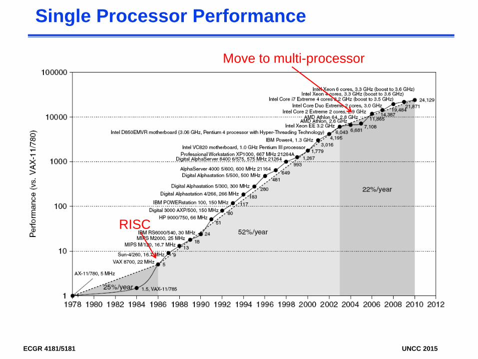
Single Processor Performance
RISC
Move to multi-processor
ECGR 4181/5181 UNCC 2015
Current Trends in Architecture
• Cannot continue to leverage Instruction-Level parallelism (ILP)Single processor performance improvement ended in
2003
• New models for performance:Data-level parallelism (DLP)Thread-level parallelism (TLP)Request-level parallelism (RLP)
• These require explicit restructuring of the application
ECGR 4181/5181 UNCC 2015
Classes of Computers• Personal Mobile Device (PMD)
e.g. smart phones, tablet computers Emphasis on cost, energy efficiency, media performance, and real-time
• Desktop Computing Emphasis on price-performance, energy, graphics
• Servers Emphasis on availability, scalability, throughput, energy
• Clusters / Warehouse Scale Computers Used for “Software as a Service (SaaS)” Emphasis on availability, price-performance, energy proportionality Sub-class: Supercomputers, emphasis: floating-point performance and
fast internal networks
• Embedded Computers Emphasis: price
ECGR 4181/5181 UNCC 2015
Embedded Processor CharacteristicsThe largest class of computers spanning the widest range
of applications and performance
• Often have minimum performance requirements. Example?
• Often have stringent limitations on cost. Example?
• Often have stringent limitations on power consumption. Example?
• Often have low tolerance for failure. Example?

ECGR 4181/5181 UNCC 2015
Characteristics of Each Segment
• Desktop: Need high performance (graphics performance?)and low price
• Servers: Need high throughput, availability (revenuelosses of $14K-$6.5M per hour of downtime), scalability
• Embedded: Need low power, low cost, low memory (almostdon’t care for performance, except real-time constraints)
Feature Desktop Server Embedded
System price $1000 - $10,000 $10,000 - $10,000,000 $10 - $100,000
Processor price $100 - $1000 $200 - $2000 $0.20 - $200
Design issues Price-perf, graphics Throughput, availability, scalability
Price, power, app-specific performance
ECGR 4181/5181 UNCC 2015
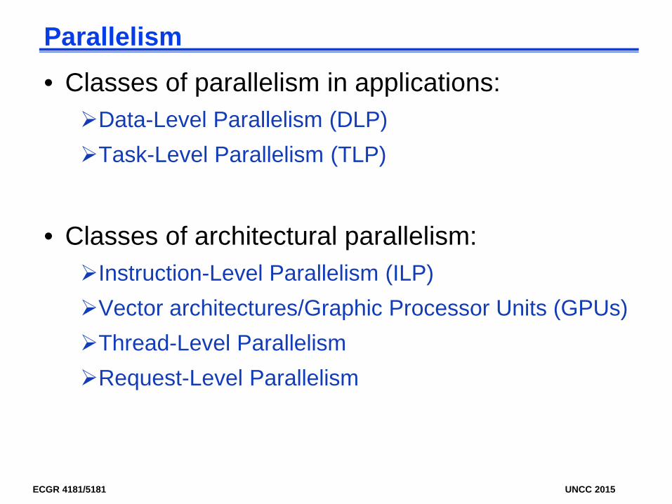
Parallelism
• Classes of parallelism in applications:Data-Level Parallelism (DLP)Task-Level Parallelism (TLP)
• Classes of architectural parallelism:Instruction-Level Parallelism (ILP)Vector architectures/Graphic Processor Units (GPUs)Thread-Level ParallelismRequest-Level Parallelism

ECGR 4181/5181 UNCC 2015
Flynn’s Taxonomy• Single instruction stream, single data stream (SISD)
• Single instruction stream, multiple data streams (SIMD)Vector architecturesMultimedia extensionsGraphics processor units
• Multiple instruction streams, single data stream (MISD)No commercial implementation
• Multiple instruction streams, multiple data streams (MIMD)Tightly-coupled MIMD Loosely-coupled MIMD

ECGR 4181/5181 UNCC 2015
Defining Computer Architecture
• “Old” view of computer architecture:Instruction Set Architecture (ISA) designi.e. decisions regarding:
- registers, memory addressing, addressing modes, instruction operands, available operations, control flow instructions, instruction encoding
• “Real” computer architecture:Specific requirements of the target machineDesign to maximize performance within constraints:
cost, power, and availabilityIncludes ISA, microarchitecture, hardware
ECGR 4181/5181 UNCC 2015
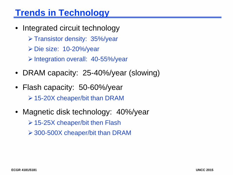
Trends in Technology• Integrated circuit technology
Transistor density: 35%/yearDie size: 10-20%/year Integration overall: 40-55%/year
• DRAM capacity: 25-40%/year (slowing)
• Flash capacity: 50-60%/year 15-20X cheaper/bit than DRAM
• Magnetic disk technology: 40%/year 15-25X cheaper/bit then Flash 300-500X cheaper/bit than DRAM
ECGR 4181/5181 UNCC 2015
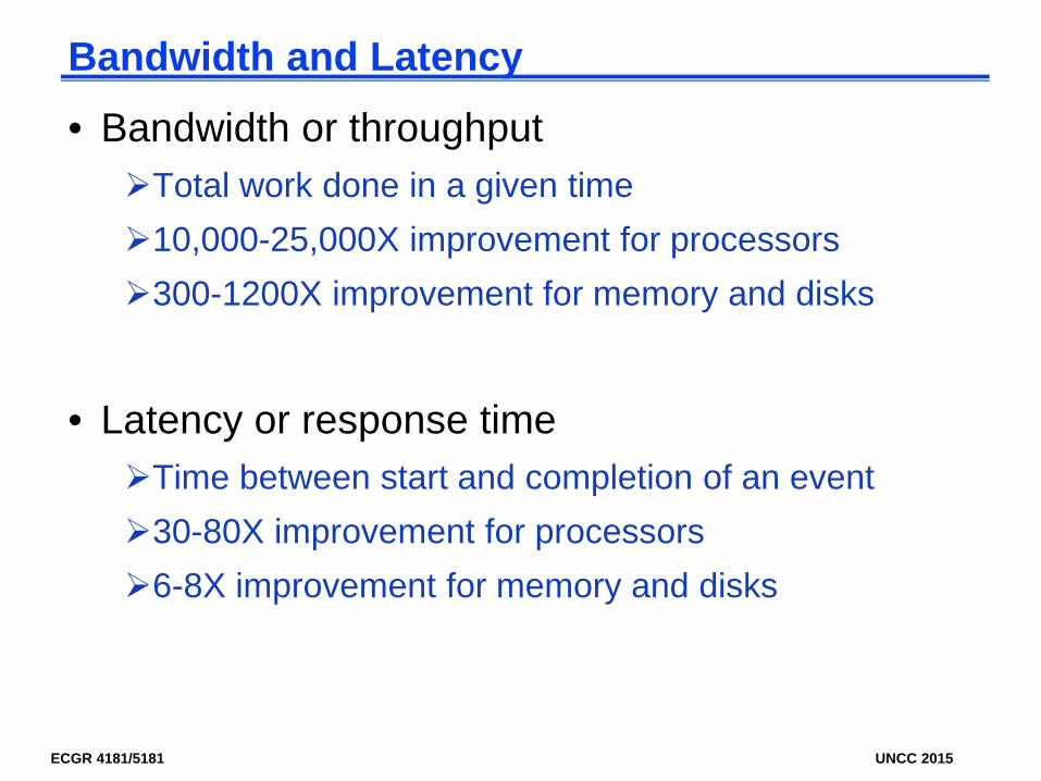
Bandwidth and Latency
• Bandwidth or throughputTotal work done in a given time10,000-25,000X improvement for processors300-1200X improvement for memory and disks
• Latency or response timeTime between start and completion of an event30-80X improvement for processors6-8X improvement for memory and disks
ECGR 4181/5181 UNCC 2015
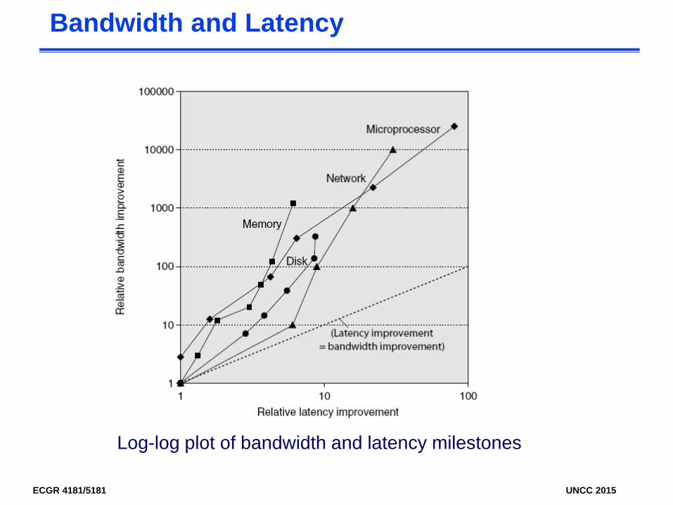
Bandwidth and Latency
Log-log plot of bandwidth and latency milestones
ECGR 4181/5181 UNCC 2015
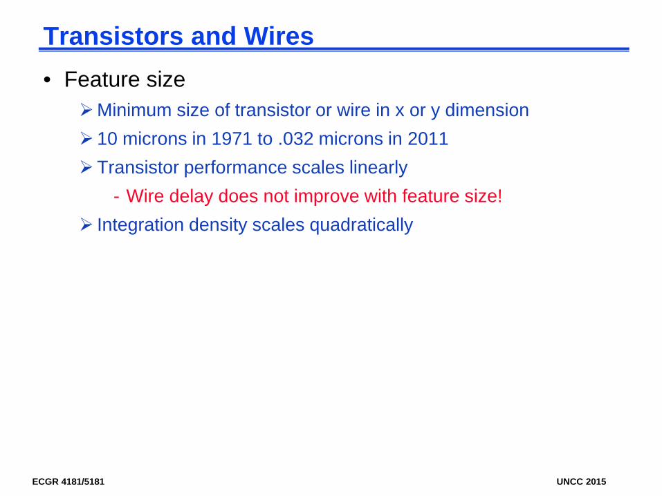
Transistors and Wires• Feature size
Minimum size of transistor or wire in x or y dimension 10 microns in 1971 to .032 microns in 2011Transistor performance scales linearly
- Wire delay does not improve with feature size! Integration density scales quadratically
ECGR 4181/5181 UNCC 2015
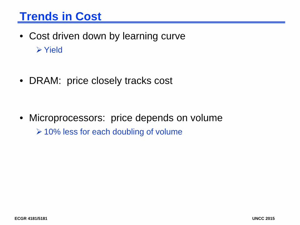
Trends in Cost• Cost driven down by learning curve
Yield
• DRAM: price closely tracks cost
• Microprocessors: price depends on volume 10% less for each doubling of volume

ECGR 4181/5181 UNCC 2015
Integrated Circuit Cost• Integrated circuit
• Bose-Einstein formula:
• Defects per unit area = 0.016-0.057 defects per square cm (2010)
• N = process-complexity factor = 11.5-15.5 (40 nm, 2010)
ECGR 4181/5181 UNCC 2015
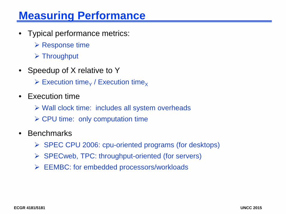
Measuring Performance• Typical performance metrics:
Response time Throughput
• Speedup of X relative to Y Execution timeY / Execution timeX
• Execution time Wall clock time: includes all system overheads CPU time: only computation time
• Benchmarks SPEC CPU 2006: cpu-oriented programs (for desktops) SPECweb, TPC: throughput-oriented (for servers) EEMBC: for embedded processors/workloads
ECGR 4181/5181 UNCC 2015
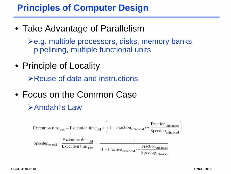
Principles of Computer Design
• Take Advantage of Parallelisme.g. multiple processors, disks, memory banks,
pipelining, multiple functional units
• Principle of LocalityReuse of data and instructions
• Focus on the Common CaseAmdahl’s Law

ECGR 4181/5181 UNCC 2015
Compute Speedup – Amdahl’s Law
Speedup is due to enhancement(E):
TimeBefore
TimeAfter
= ExTimebefore x [(1-F) + FS ]
Speedup(E) =ExTimebefore
ExTimeafter
=1
FS
][(1-F) +
Let F be the fraction where enhancement is applied => Also, called parallel fraction and (1-F) as the serial fraction
Execution timeafter
ECGR 4181/5181 UNCC 2015
Principles of Computer Design
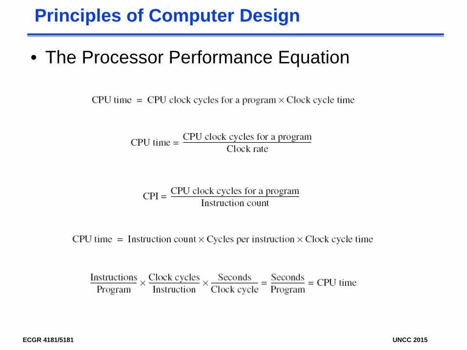
• The Processor Performance Equation
ECGR 4181/5181 UNCC 2015
Principles of Computer Design
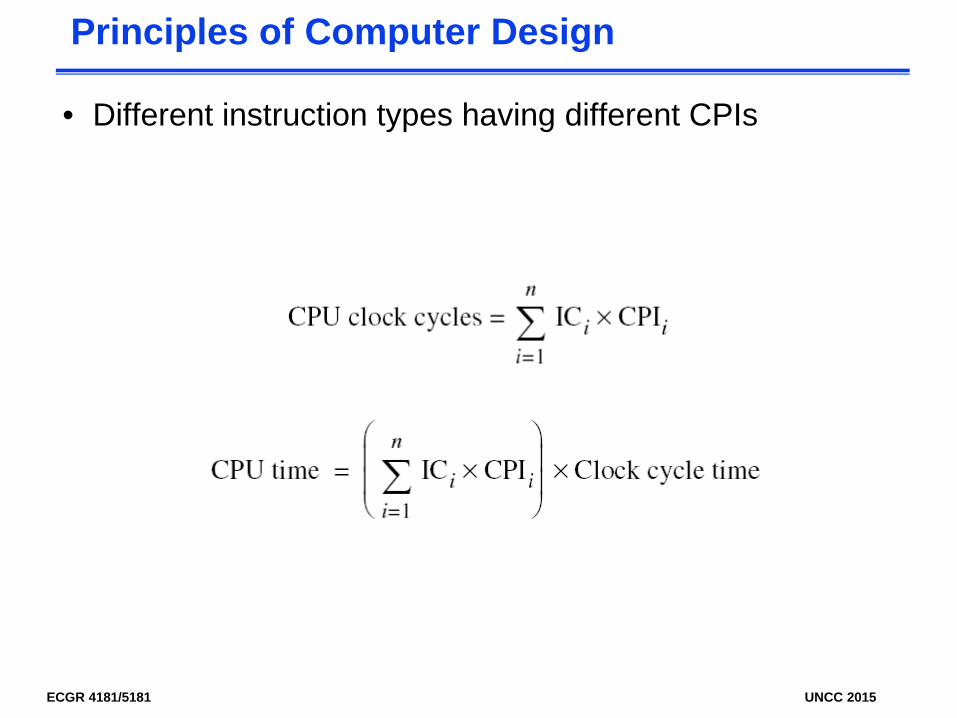
• Different instruction types having different CPIs

ECGR 4181/5181 UNCC 2015
Measuring Performance
How do we conclude that System-A is “better” thanSystem-B?
ECGR 4181/5181 UNCC 2015
Performance Metrics• Purchasing perspective
given a collection of machines, which has the– best performance?– least cost?– best cost/performance?
• Design perspective faced with design options, which has the
– best performance improvement?– least cost?– best cost/performance?
• Both require basis for comparisonmetric for evaluation
• Our goal is to understand what factors in the architecture contribute to overall system performance and the relative importance (and cost) of these factors
ECGR 4181/5181 UNCC 2015
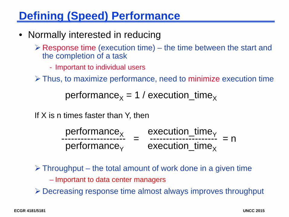
Defining (Speed) Performance• Normally interested in reducing
Response time (execution time) – the time between the start and the completion of a task
- Important to individual usersThus, to maximize performance, need to minimize execution time
Throughput – the total amount of work done in a given time– Important to data center managers
Decreasing response time almost always improves throughput
performanceX = 1 / execution_timeX
If X is n times faster than Y, then
performanceX execution_timeY -------------------- = --------------------- = nperformanceY execution_timeX
ECGR 4181/5181 UNCC 2015
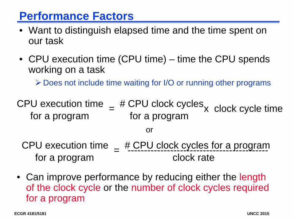
Performance Factors• Want to distinguish elapsed time and the time spent on
our task
• CPU execution time (CPU time) – time the CPU spends working on a taskDoes not include time waiting for I/O or running other programs
CPU execution time # CPU clock cyclesfor a program for a program
= x clock cycle time
CPU execution time # CPU clock cycles for a programfor a program clock rate
= -------------------------------------------
• Can improve performance by reducing either the length of the clock cycle or the number of clock cycles required for a program
or
ECGR 4181/5181 UNCC 2015
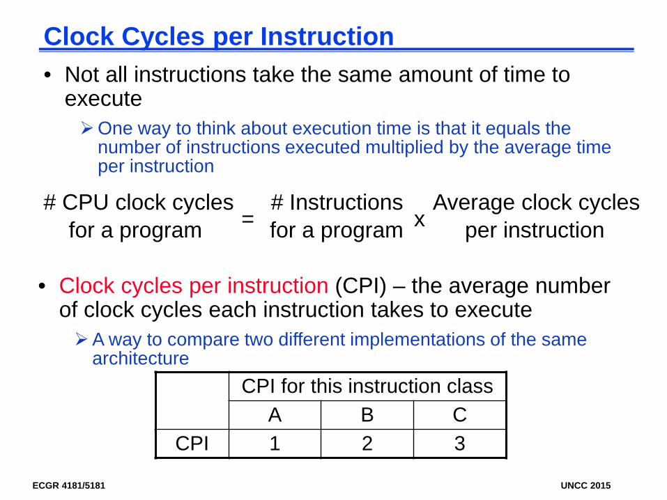
Clock Cycles per Instruction• Not all instructions take the same amount of time to
executeOne way to think about execution time is that it equals the
number of instructions executed multiplied by the average time per instruction
• Clock cycles per instruction (CPI) – the average number of clock cycles each instruction takes to executeA way to compare two different implementations of the same
architecture
# CPU clock cycles # Instructions Average clock cyclesfor a program for a program per instruction = x
CPI for this instruction classA B C
CPI 1 2 3
ECGR 4181/5181 UNCC 2015
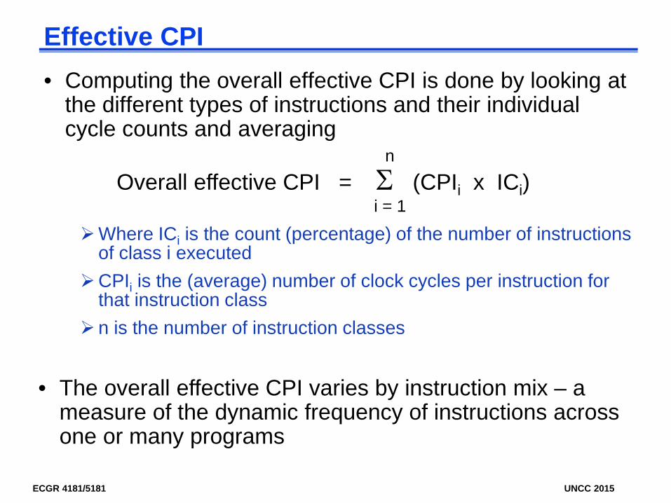
Effective CPI• Computing the overall effective CPI is done by looking at
the different types of instructions and their individual cycle counts and averaging
Overall effective CPI = Σ (CPIi x ICi)i = 1
n
Where ICi is the count (percentage) of the number of instructions of class i executed
CPIi is the (average) number of clock cycles per instruction for that instruction class
n is the number of instruction classes
• The overall effective CPI varies by instruction mix – a measure of the dynamic frequency of instructions across one or many programs
ECGR 4181/5181 UNCC 2015
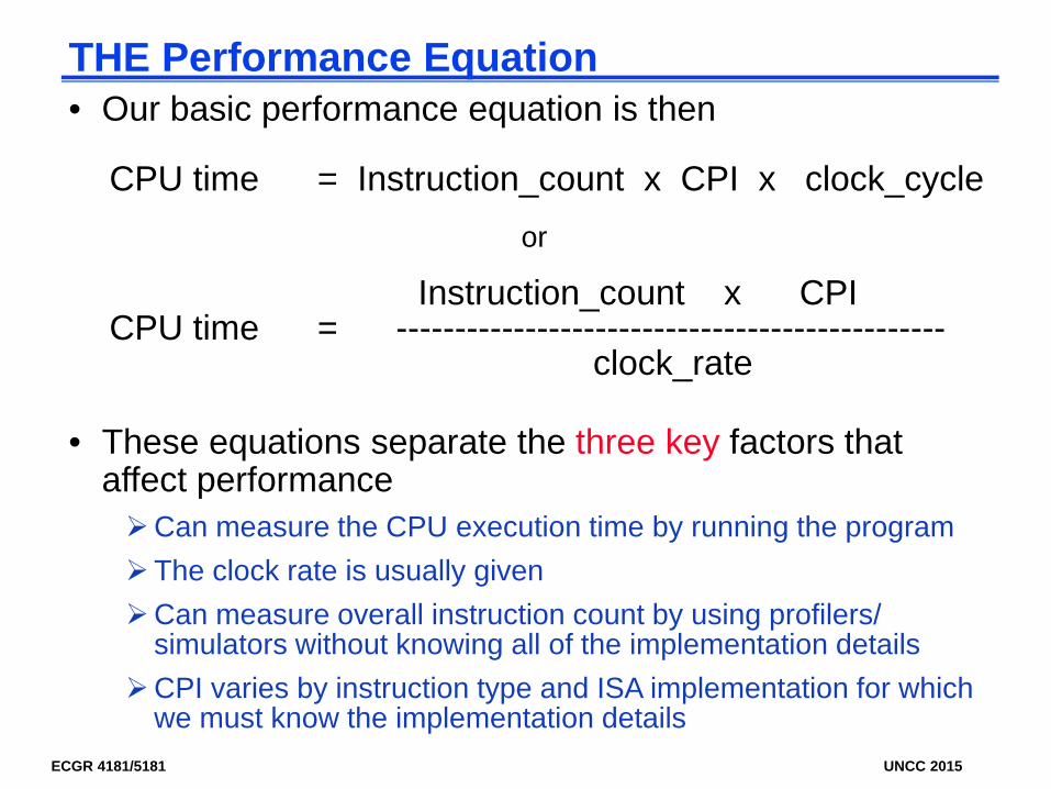
THE Performance Equation• Our basic performance equation is then
CPU time = Instruction_count x CPI x clock_cycle
Instruction_count x CPI
clock_rate CPU time = -----------------------------------------------
or
• These equations separate the three key factors that affect performanceCan measure the CPU execution time by running the programThe clock rate is usually givenCan measure overall instruction count by using profilers/
simulators without knowing all of the implementation detailsCPI varies by instruction type and ISA implementation for which
we must know the implementation details
ECGR 4181/5181 UNCC 2015
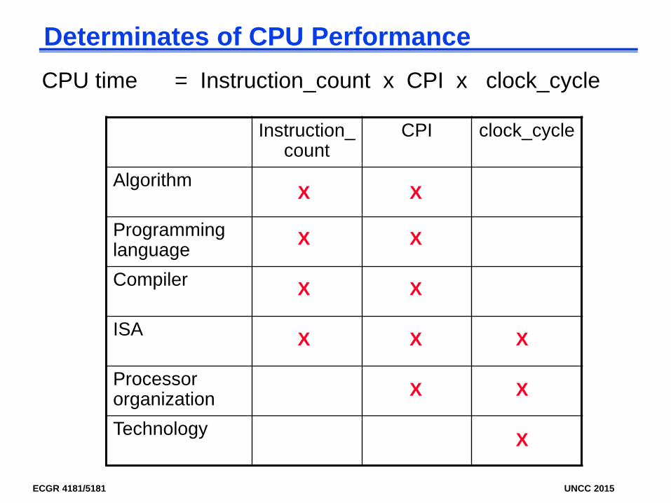
Determinates of CPU PerformanceCPU time = Instruction_count x CPI x clock_cycle
Instruction_count
CPI clock_cycle
Algorithm
Programming languageCompiler
ISA
Processor organizationTechnology X
XX
XX
X X
X
X
X
X
X

ECGR 4181/5181 UNCC 2015
A Simple Example
• How much faster would the machine be if a better data cache reduced the average load time to 2 cycles?
• How does this compare with using branch prediction to shave a cycle off the branch time?
• What if two ALU instructions could be executed at once?
Op Freq CPIi Freq x CPIiALU 50% 1
Load 20% 5
Store 10% 3
Branch 20% 2
Σ =
.5
1.0
.3
.4
2.2
CPU time new = 1.6 x IC x CC so 2.2/1.6 means 37.5% faster
1.6
.5
.4
.3
.4
.5
1.0
.3
.2
2.0
CPU time new = 2.0 x IC x CC so 2.2/2.0 means 10% faster
.25
1.0
.3
.4
1.95
CPU time new = 1.95 x IC x CC so 2.2/1.95 means 12.8% faster
ECGR 4181/5181 UNCC 2015
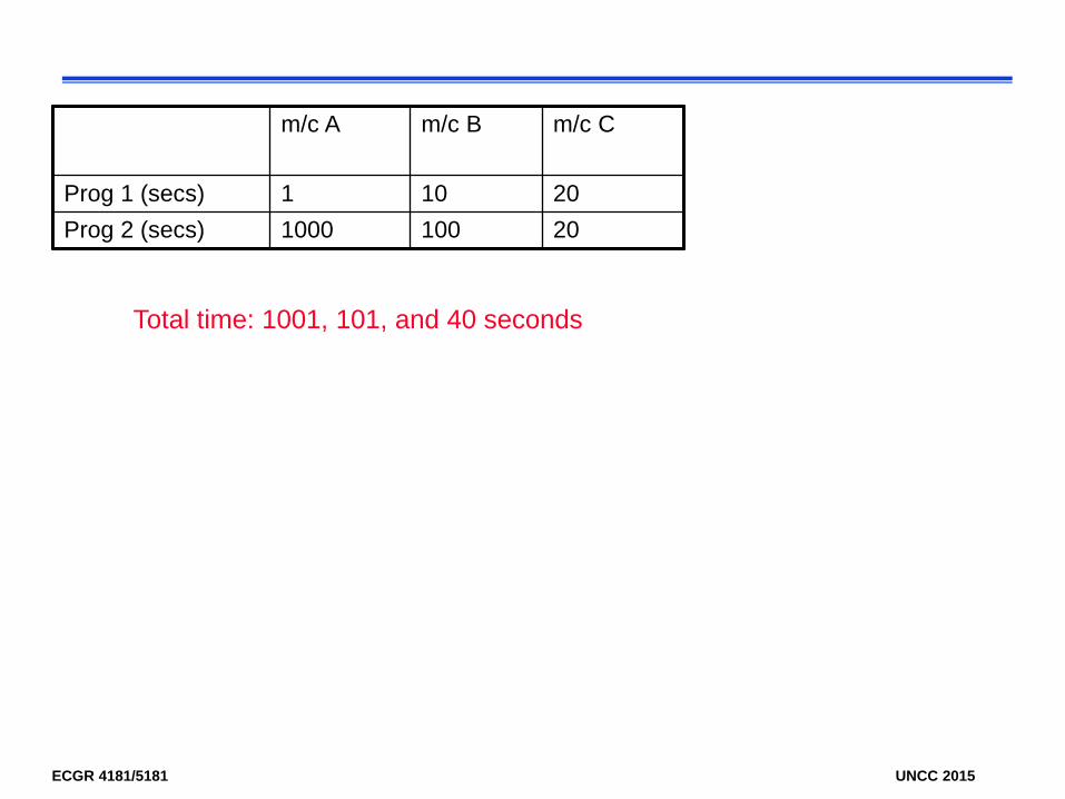
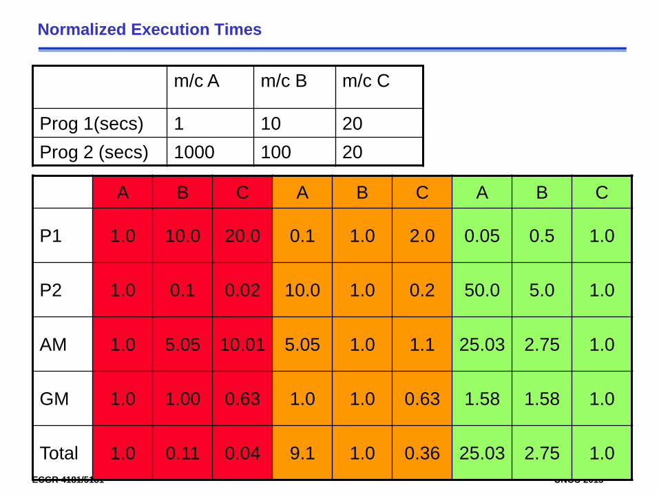
m/c A m/c B m/c C
Prog 1 (secs) 1 10 20Prog 2 (secs) 1000 100 20
Total time: 1001, 101, and 40 seconds
ECGR 4181/5181 UNCC 2015
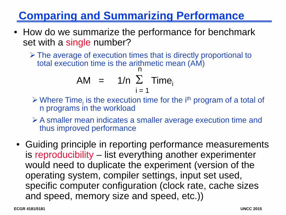
Comparing and Summarizing Performance
• Guiding principle in reporting performance measurements is reproducibility – list everything another experimenter would need to duplicate the experiment (version of the operating system, compiler settings, input set used, specific computer configuration (clock rate, cache sizes and speed, memory size and speed, etc.))
• How do we summarize the performance for benchmark set with a single number?The average of execution times that is directly proportional to
total execution time is the arithmetic mean (AM)
AM = 1/n Σ Timeii = 1
n
Where Timei is the execution time for the ith program of a total of n programs in the workload
A smaller mean indicates a smaller average execution time and thus improved performance
ECGR 4181/5181 UNCC 2015
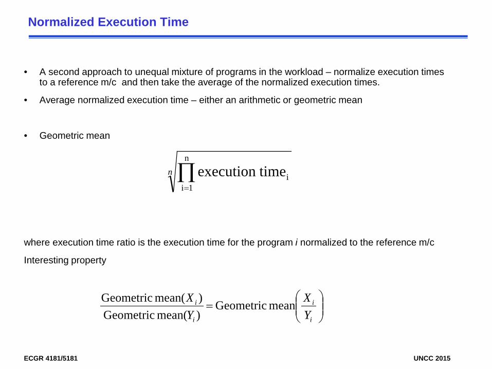
Normalized Execution Time
• A second approach to unequal mixture of programs in the workload – normalize execution times to a reference m/c and then take the average of the normalized execution times.
• Average normalized execution time – either an arithmetic or geometric mean
• Geometric mean
where execution time ratio is the execution time for the program i normalized to the reference m/c
Interesting property
n ∏=
n
1iitimeexecution
=
i
i
i
i
YX
YX mean Geometric
)mean( Geometric)mean( Geometric

ECGR 4181/5181 UNCC 2015
Normalized Execution Times
• Geometric means of normalized execution times are consistent - does not matter which m/c is the reference
• Not true for arithmetic mean – should not be used to average normalized execution times
• Weighted arithmetic means – weightings are proportional to execution times – influenced by frequency of use in workload, type of m/c, and size of program input. Geometric mean is independent of running times of individual programs and any m/c can be used for normalization
• Example: Comparative performance evaluation where programs were fixed and inputs are not Competitors could calculate weighted arithmetic mean by using their best performing
benchmark for the longest input. Geometric mean would be less misleading than arithmetic mean for such situations
ECGR 4181/5181 UNCC 2015
Normalized Execution Times
A B C A B C A B C
P1 1.0 10.0 20.0 0.1 1.0 2.0 0.05 0.5 1.0
P2 1.0 0.1 0.02 10.0 1.0 0.2 50.0 5.0 1.0
AM 1.0 5.05 10.01 5.05 1.0 1.1 25.03 2.75 1.0
GM 1.0 1.00 0.63 1.0 1.0 0.63 1.58 1.58 1.0
Total 1.0 0.11 0.04 9.1 1.0 0.36 25.03 2.75 1.0
m/c A m/c B m/c C
Prog 1(secs) 1 10 20Prog 2 (secs) 1000 100 20
ECGR 4181/5181 UNCC 2015
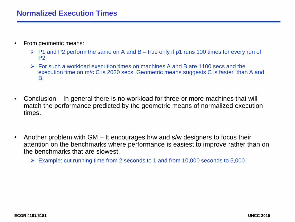
Normalized Execution Times
• From geometric means: P1 and P2 perform the same on A and B – true only if p1 runs 100 times for every run of
P2 For such a workload execution times on machines A and B are 1100 secs and the
execution time on m/c C is 2020 secs. Geometric means suggests C is faster than A and B.
• Conclusion – In general there is no workload for three or more machines that will match the performance predicted by the geometric means of normalized execution times.
• Another problem with GM – It encourages h/w and s/w designers to focus their attention on the benchmarks where performance is easiest to improve rather than on the benchmarks that are slowest. Example: cut running time from 2 seconds to 1 and from 10,000 seconds to 5,000
ECGR 4181/5181 UNCC 2015
Example
• A new laptop has an IPC that is 20% worse than the oldlaptop. It has a clock speed that is 30% higher than the oldlaptop. The same binaries on both machines.What is the speedup of the new laptop?
ECGR 4181/5181 UNCC 2015
Example
• A new laptop has an IPC that is 20% worse than the oldlaptop. It has a clock speed that is 30% higher than the oldlaptop. The same binaries on both machines.Their IPCs are listed below. The binaries are run such that each binary gets an equal share of CPU time.What is the speedup of the new laptop?
P1 P2 P3Old-IPC 1.2 1.6 2.0New-IPC 1.6 1.6 1.6
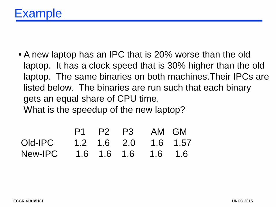
ECGR 4181/5181 UNCC 2015
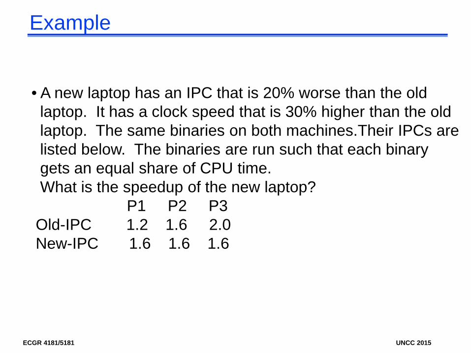
Example
• A new laptop has an IPC that is 20% worse than the oldlaptop. It has a clock speed that is 30% higher than the oldlaptop. The same binaries on both machines.Their IPCs are listed below. The binaries are run such that each binary gets an equal share of CPU time.What is the speedup of the new laptop?
P1 P2 P3 AM GMOld-IPC 1.2 1.6 2.0 1.6 1.57New-IPC 1.6 1.6 1.6 1.6 1.6
ECGR 4181/5181 UNCC 2015
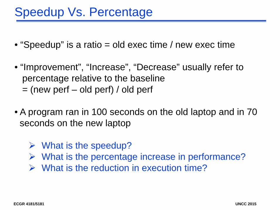
Speedup Vs. Percentage
• “Speedup” is a ratio = old exec time / new exec time
• “Improvement”, “Increase”, “Decrease” usually refer topercentage relative to the baseline = (new perf – old perf) / old perf
• A program ran in 100 seconds on the old laptop and in 70seconds on the new laptop
What is the speedup? What is the percentage increase in performance? What is the reduction in execution time?
ECGR 4181/5181 UNCC 2015
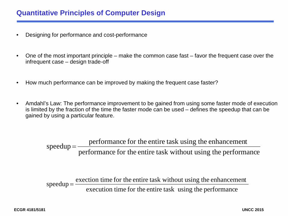
Quantitative Principles of Computer Design
• Designing for performance and cost-performance
• One of the most important principle – make the common case fast – favor the frequent case over the infrequent case – design trade-off
• How much performance can be improved by making the frequent case faster?
• Amdahl’s Law: The performance improvement to be gained from using some faster mode of execution is limited by the fraction of the time the faster mode can be used – defines the speedup that can be gained by using a particular feature.
eperformanc theusingout task withentire for the eperformanct enhancemen theusing task entire for the eperformanc speedup =
eperformanc theusing task entire for the timeexecution t enhancemen theusingout task withentire for the imeexection t speedup =
ECGR 4181/5181 UNCC 2015
Quantitative Principles of Computer Design
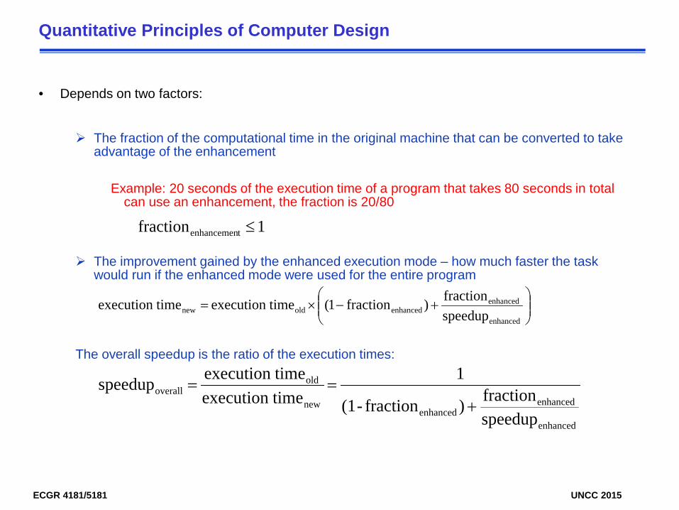
• Depends on two factors:
The fraction of the computational time in the original machine that can be converted to take advantage of the enhancement
Example: 20 seconds of the execution time of a program that takes 80 seconds in total can use an enhancement, the fraction is 20/80
The improvement gained by the enhanced execution mode – how much faster the task would run if the enhanced mode were used for the entire program
The overall speedup is the ratio of the execution times:
1fraction tenhancemen ≤
+−×=
enhanced
enhancedenhancedoldnew speedup
fraction )fraction 1(timeexecution timeexecution
enhanced
enhancedenhanced
new
oldoverall
speedupfraction )fraction-(1
1 timeexecution timeexecution speedup
+==
ECGR 4181/5181 UNCC 2015
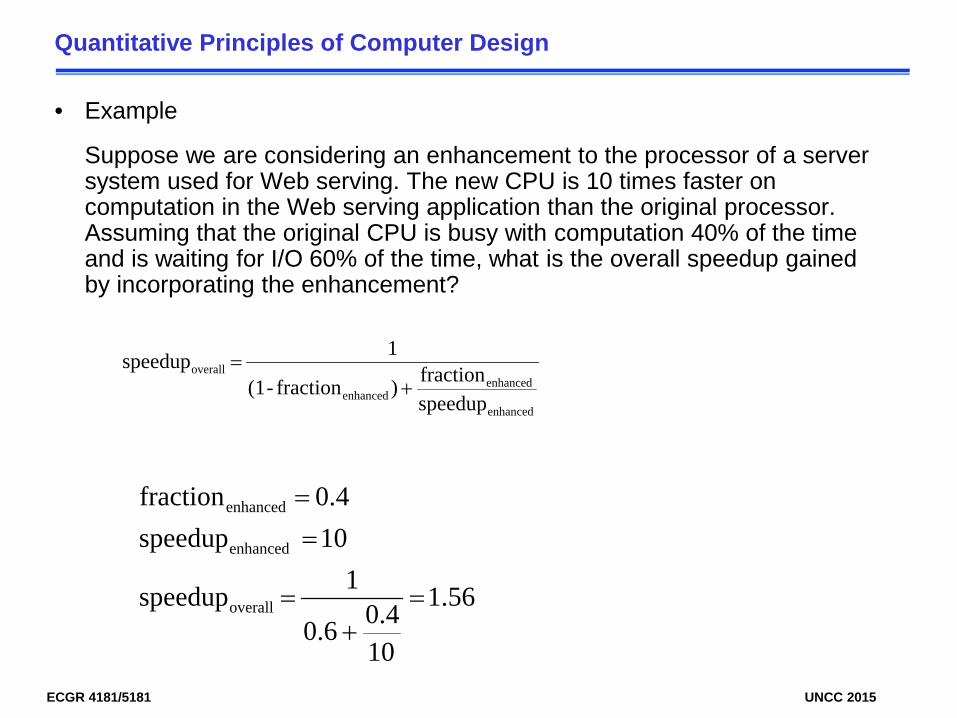
Quantitative Principles of Computer Design
• Example
Suppose we are considering an enhancement to the processor of a server system used for Web serving. The new CPU is 10 times faster on computation in the Web serving application than the original processor. Assuming that the original CPU is busy with computation 40% of the time and is waiting for I/O 60% of the time, what is the overall speedup gained by incorporating the enhancement?
enhanced
enhancedenhanced
overall
speedupfraction )fraction-(1
1 speedup+
=
1.56
100.4 0.6
1 speedup
10 speedup0.4 fraction
overall
enhanced
enhanced
=+
=
==
ECGR 4181/5181 UNCC 2015
Quantitative Principles of Computer Design
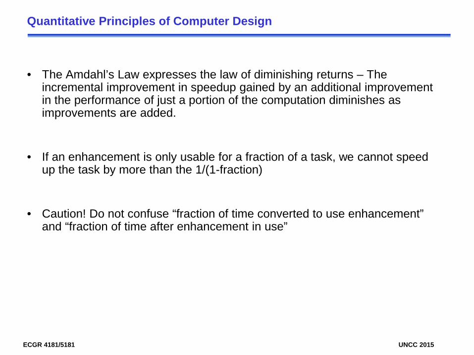
• The Amdahl’s Law expresses the law of diminishing returns – The incremental improvement in speedup gained by an additional improvement in the performance of just a portion of the computation diminishes as improvements are added.
• If an enhancement is only usable for a fraction of a task, we cannot speed up the task by more than the 1/(1-fraction)
• Caution! Do not confuse “fraction of time converted to use enhancement” and “fraction of time after enhancement in use”
ECGR 4181/5181 UNCC 2015
Quantitative Principles of Computer Design
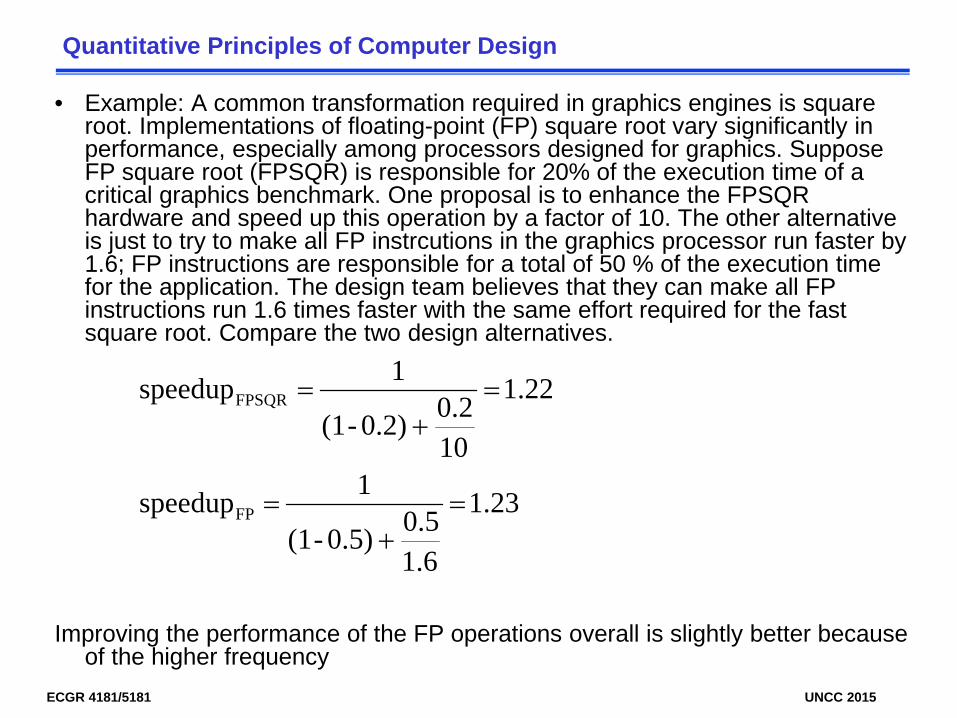
• Example: A common transformation required in graphics engines is square root. Implementations of floating-point (FP) square root vary significantly in performance, especially among processors designed for graphics. Suppose FP square root (FPSQR) is responsible for 20% of the execution time of a critical graphics benchmark. One proposal is to enhance the FPSQR hardware and speed up this operation by a factor of 10. The other alternative is just to try to make all FP instrcutions in the graphics processor run faster by 1.6; FP instructions are responsible for a total of 50 % of the execution time for the application. The design team believes that they can make all FP instructions run 1.6 times faster with the same effort required for the fast square root. Compare the two design alternatives.
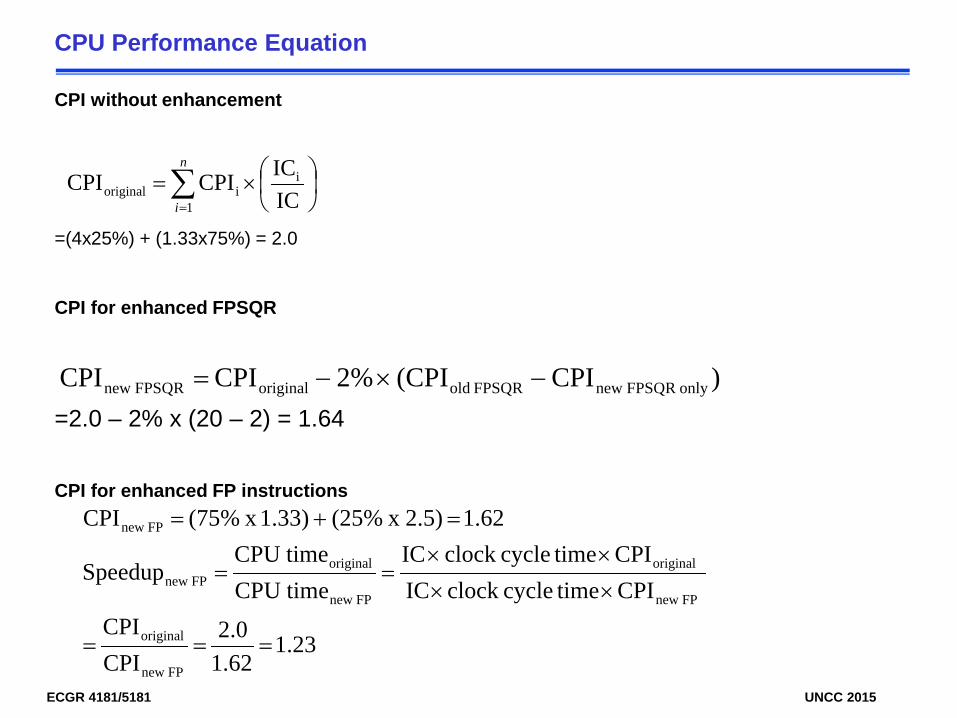
Improving the performance of the FP operations overall is slightly better because of the higher frequency
1.23
1.60.5 0.5)-(1
1 speedup
1.22
100.2 0.2)-(1
1 speedup
FP
FPSQR
=+
=
=+
=
ECGR 4181/5181 UNCC 2015
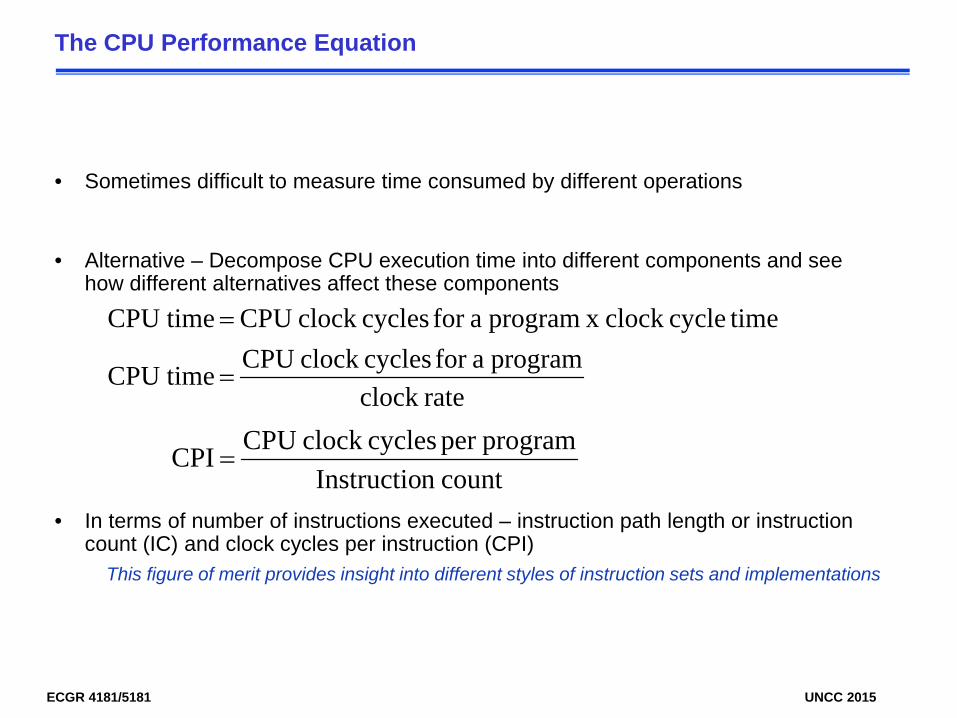
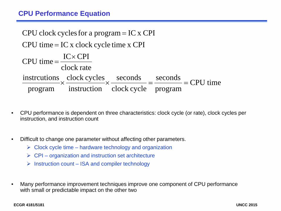
The CPU Performance Equation
• Sometimes difficult to measure time consumed by different operations
• Alternative – Decompose CPU execution time into different components and see how different alternatives affect these components
• In terms of number of instructions executed – instruction path length or instruction count (IC) and clock cycles per instruction (CPI)
This figure of merit provides insight into different styles of instruction sets and implementations
rateclock program afor cyclesclock CPU timeCPU
timecycleclock x program afor cyclesclock CPU timeCPU
=
=
countn Instructioprogramper cyclesclock CPU CPI =
ECGR 4181/5181 UNCC 2015
CPU Performance Equation
• CPU performance is dependent on three characteristics: clock cycle (or rate), clock cycles per instruction, and instruction count
• Difficult to change one parameter without affecting other parameters. Clock cycle time – hardware technology and organization CPI – organization and instruction set architecture Instruction count – ISA and compiler technology
• Many performance improvement techniques improve one component of CPU performance with small or predictable impact on the other two
timeCPUprogramseconds
cycleclock seconds
ninstructiocyclesclock
programnsinstrcutio
rateclock CPI IC timeCPU
CPI x timecycleclock x IC timeCPUCPI x IC program afor cyclesclock CPU
==××
×=
==

ECGR 4181/5181 UNCC 2015
CPU Performance Equation
• Sometimes it is useful to calculate the number of total CPU clock cycles as
• Note: should be measured and not just calculated from the reference table
• Possible uses of CPU performance equation: High-level performance comparisons Back-of-the-envelope calculations Enable architects to think about compilers and technology
i
n
1i
i
n
1iii
n
1iii
i
n
1ii
CPIICIC
IC
CPIIC CPI
timecycle clockCPIIC time CPU
CPIIC cycles clock CPU
×=×
=
×
×=
×=
∑∑
∑
∑
=
=
=
=
iCPI
ECGR 4181/5181 UNCC 2015
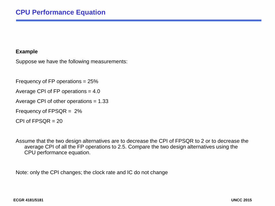
CPU Performance Equation
Example
Suppose we have the following measurements:
Frequency of FP operations = 25%
Average CPI of FP operations = 4.0
Average CPI of other operations = 1.33
Frequency of FPSQR = 2%
CPI of FPSQR = 20
Assume that the two design alternatives are to decrease the CPI of FPSQR to 2 or to decrease the average CPI of all the FP operations to 2.5. Compare the two design alternatives using the CPU performance equation.
Note: only the CPI changes; the clock rate and IC do not change
ECGR 4181/5181 UNCC 2015
CPU Performance Equation
CPI without enhancement
=(4x25%) + (1.33x75%) = 2.0
CPI for enhanced FPSQR
=2.0 – 2% x (20 – 2) = 1.64
CPI for enhanced FP instructions
×=∑
= ICICCPICPI i
1ioriginal
n
i
)CPI (CPI 2% CPI CPI only FPSQR newFPSQR oldoriginalFPSQR new −×−=
1.23 1.622.0
CPICPI
CPI timecycleclock IC CPI timecycleclock IC
timeCPU timeCPU
Speedup
1.62 2.5) x (25% 1.33) x (75% CPI
FP new
original
FP new
original
FP new
originalFP new
FP new
===
××
××==
=+=
ECGR 4181/5181 UNCC 2015
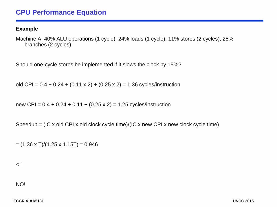
CPU Performance Equation
Example
Machine A: 40% ALU operations (1 cycle), 24% loads (1 cycle), 11% stores (2 cycles), 25% branches (2 cycles)
Should one-cycle stores be implemented if it slows the clock by 15%?
old CPI = 0.4 + 0.24 + (0.11 x 2) + (0.25 x 2) = 1.36 cycles/instruction
new CPI = 0.4 + 0.24 + 0.11 + (0.25 x 2) = 1.25 cycles/instruction
Speedup = (IC x old CPI x old clock cycle time)/(IC x new CPI x new clock cycle time)
= (1.36 x T)/(1.25 x 1.15T) = 0.946
< 1
NO!
ECGR 4181/5181 UNCC 2015
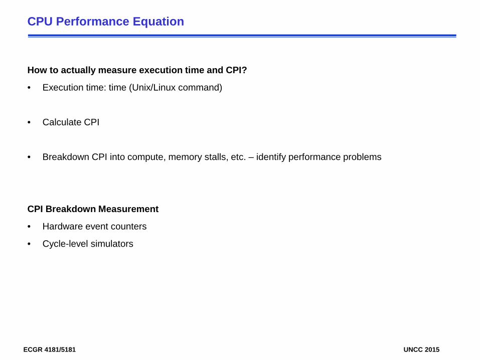
CPU Performance Equation
How to actually measure execution time and CPI?
• Execution time: time (Unix/Linux command)
• Calculate CPI
• Breakdown CPI into compute, memory stalls, etc. – identify performance problems
CPI Breakdown Measurement
• Hardware event counters
• Cycle-level simulators
ECGR 4181/5181 UNCC 2015
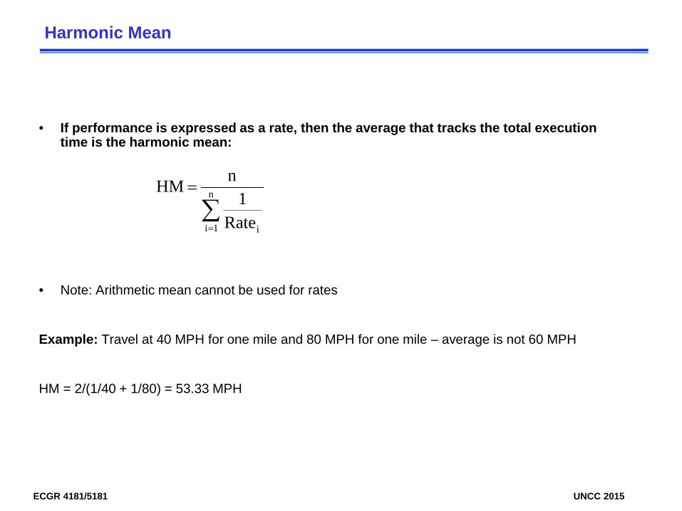
Harmonic Mean
• If performance is expressed as a rate, then the average that tracks the total execution time is the harmonic mean:
• Note: Arithmetic mean cannot be used for rates
Example: Travel at 40 MPH for one mile and 80 MPH for one mile – average is not 60 MPH
HM = 2/(1/40 + 1/80) = 53.33 MPH
∑=
= n
1i iRate1
n HM
ECGR 4181/5181 UNCC 2015
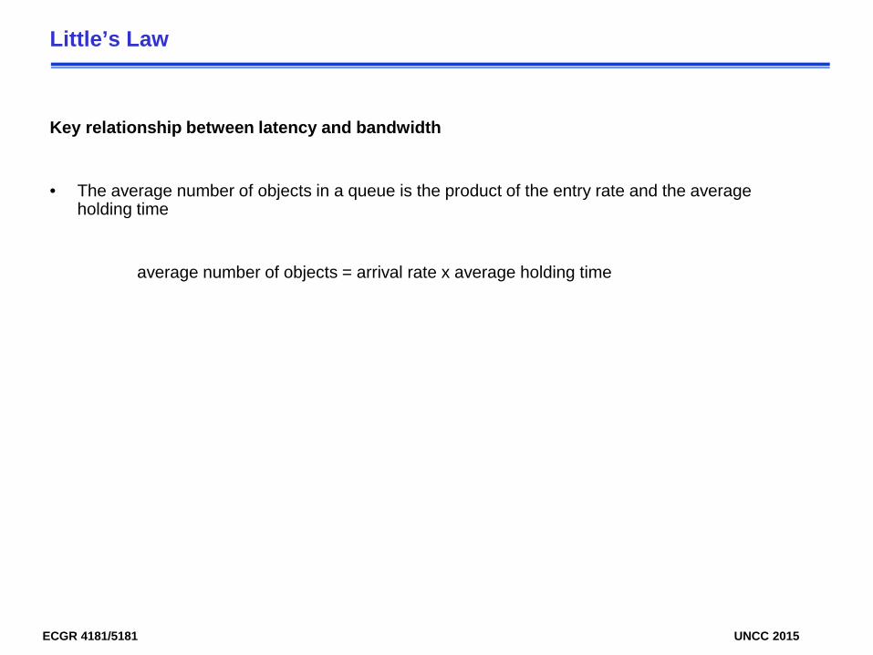
Little’s Law
Key relationship between latency and bandwidth
• The average number of objects in a queue is the product of the entry rate and the average holding time
average number of objects = arrival rate x average holding time
ECGR 4181/5181 UNCC 2015
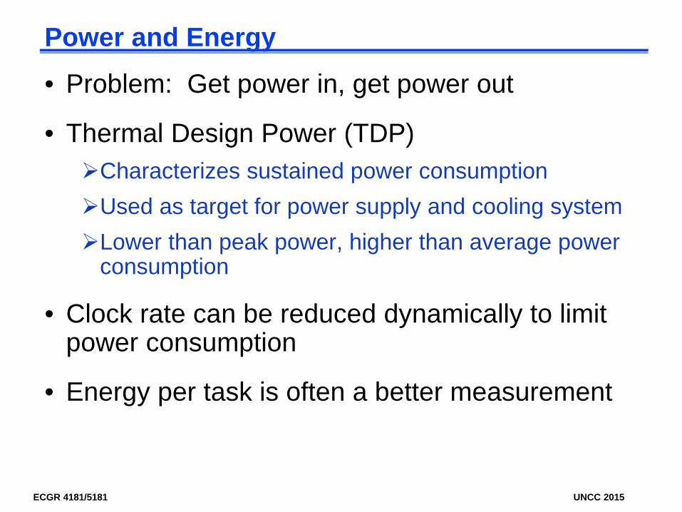
Power and Energy
• Problem: Get power in, get power out
• Thermal Design Power (TDP)Characterizes sustained power consumptionUsed as target for power supply and cooling systemLower than peak power, higher than average power
consumption
• Clock rate can be reduced dynamically to limit power consumption
• Energy per task is often a better measurement
ECGR 4181/5181 UNCC 2015
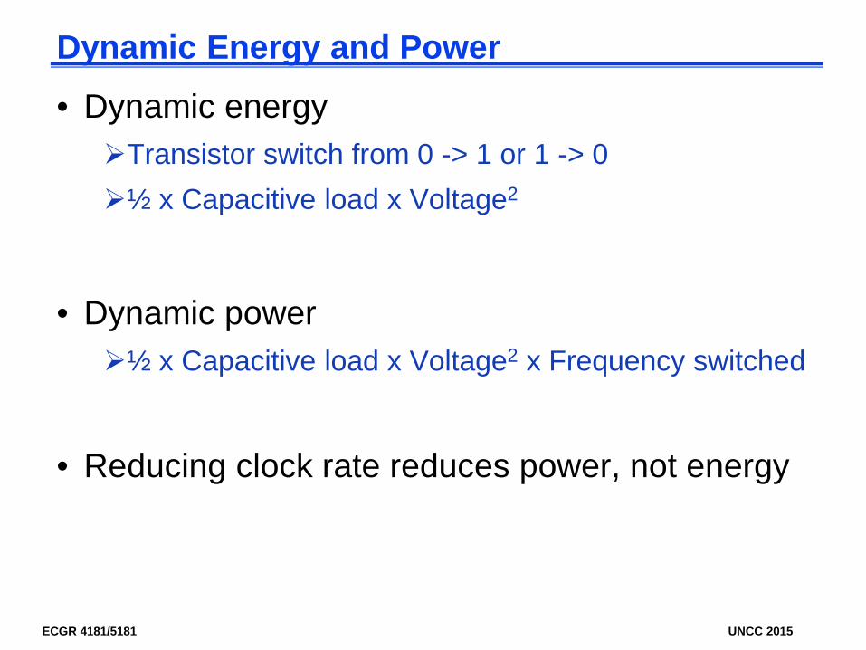
Dynamic Energy and Power
• Dynamic energyTransistor switch from 0 -> 1 or 1 -> 0½ x Capacitive load x Voltage2
• Dynamic power½ x Capacitive load x Voltage2 x Frequency switched
• Reducing clock rate reduces power, not energy

ECGR 4181/5181 UNCC 2015
Power
• Intel 80386 consumed ~ 2 W
• 3.3 GHz Intel Core i7 consumes 130 W
• Heat must be dissipated from 1.5 x 1.5 cm chip
• This is the limit of what can be cooled by air
ECGR 4181/5181 UNCC 2015
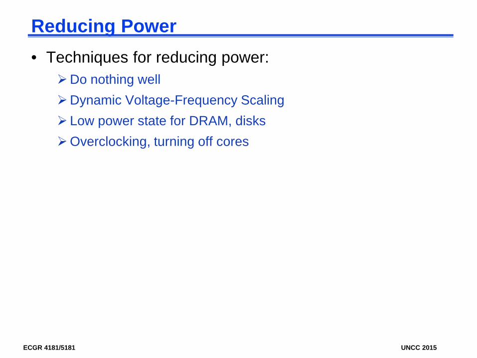
Reducing Power• Techniques for reducing power:
Do nothing wellDynamic Voltage-Frequency Scaling Low power state for DRAM, disksOverclocking, turning off cores
ECGR 4181/5181 UNCC 2015
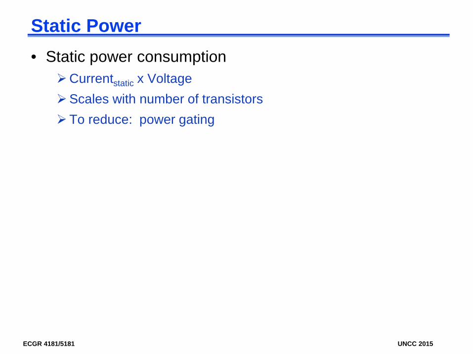
Static Power• Static power consumption
Currentstatic x VoltageScales with number of transistorsTo reduce: power gating

ECGR 4181/5181 UNCC 2015
Power Trends
• In CMOS IC technology
The Power Wall
FrequencyVoltageload CapacitivePower 2 ××=
×1000×30 5V → 1V
ECGR 4181/5181 UNCC 2015
Reducing Power
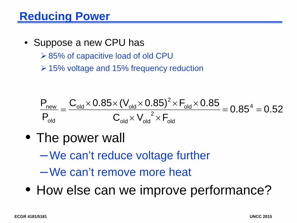
• Suppose a new CPU has 85% of capacitive load of old CPU 15% voltage and 15% frequency reduction
0.520.85FVC
0.85F0.85)(V0.85CPP 4
old2
oldold
old2
oldold
old
new ==××
×××××=
• The power wall–We can’t reduce voltage further–We can’t remove more heat
• How else can we improve performance?
ECGR 4181/5181 UNCC 2015
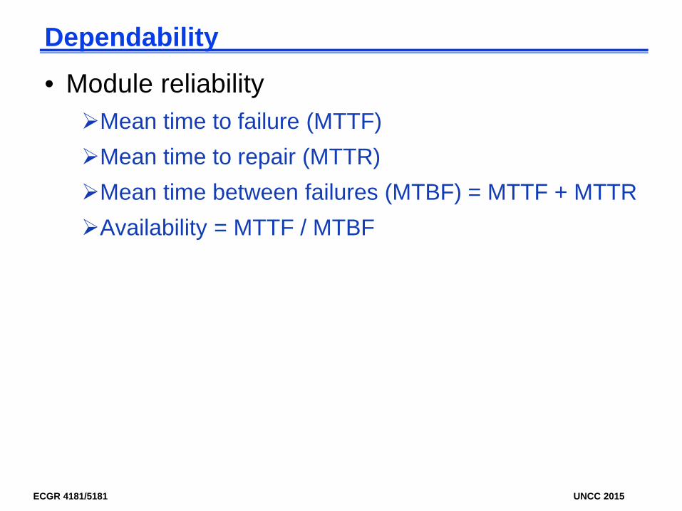
Dependability
• Module reliabilityMean time to failure (MTTF)Mean time to repair (MTTR)Mean time between failures (MTBF) = MTTF + MTTRAvailability = MTTF / MTBF
ECGR 4181/5181 UNCC 2015
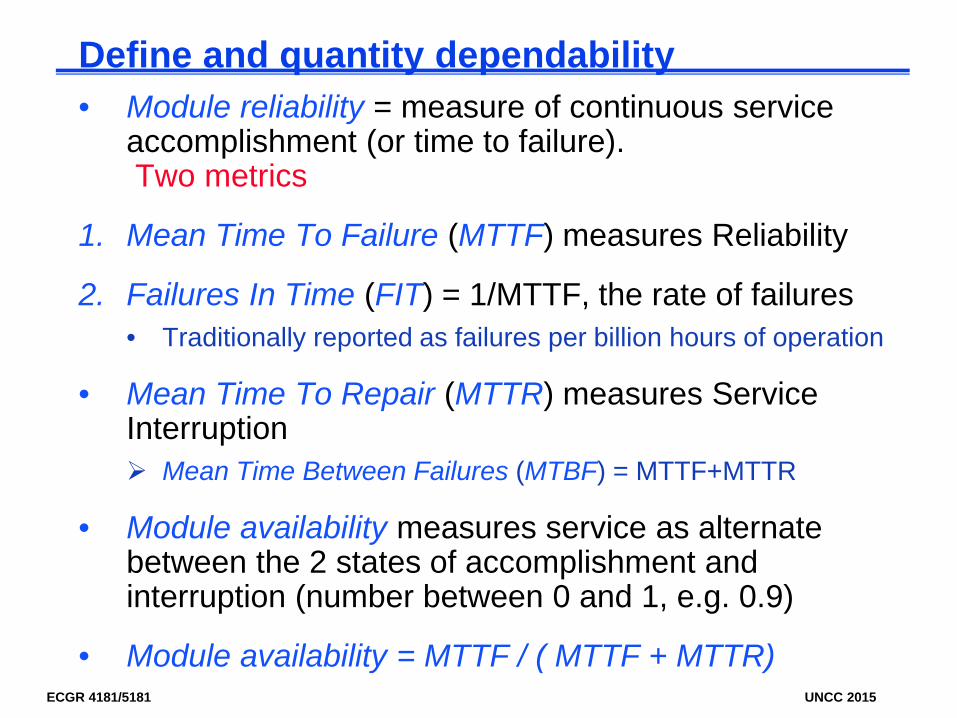
Define and quantity dependability • Module reliability = measure of continuous service
accomplishment (or time to failure).Two metrics
1. Mean Time To Failure (MTTF) measures Reliability
2. Failures In Time (FIT) = 1/MTTF, the rate of failures • Traditionally reported as failures per billion hours of operation
• Mean Time To Repair (MTTR) measures Service Interruption Mean Time Between Failures (MTBF) = MTTF+MTTR
• Module availability measures service as alternate between the 2 states of accomplishment and interruption (number between 0 and 1, e.g. 0.9)
• Module availability = MTTF / ( MTTF + MTTR)
ECGR 4181/5181 UNCC 2015
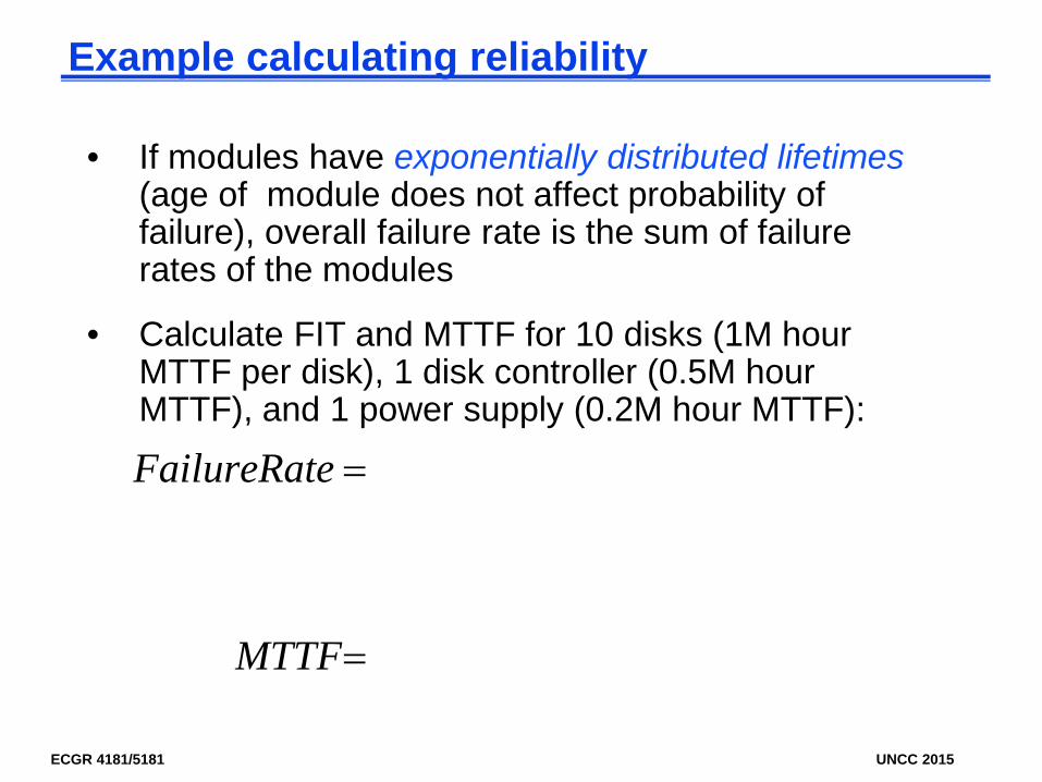
Example calculating reliability
• If modules have exponentially distributed lifetimes(age of module does not affect probability of failure), overall failure rate is the sum of failure rates of the modules
• Calculate FIT and MTTF for 10 disks (1M hour MTTF per disk), 1 disk controller (0.5M hour MTTF), and 1 power supply (0.2M hour MTTF):
=
=
MTTF
eFailureRat
ECGR 4181/5181 UNCC 2015
Performance Improvement
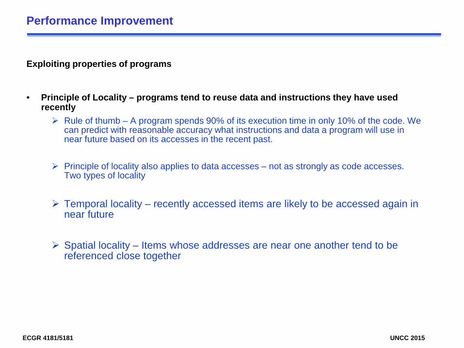
Exploiting properties of programs
• Principle of Locality – programs tend to reuse data and instructions they have used recently Rule of thumb – A program spends 90% of its execution time in only 10% of the code. We
can predict with reasonable accuracy what instructions and data a program will use in near future based on its accesses in the recent past.
Principle of locality also applies to data accesses – not as strongly as code accesses. Two types of locality
Temporal locality – recently accessed items are likely to be accessed again in near future
Spatial locality – Items whose addresses are near one another tend to be referenced close together

ECGR 4181/5181 UNCC 2015
Performance Improvement
Take Advantage of Parallelism
• One of the most important methods for improving performance
• Parallelism at different levels. For example, System level – multiprocessors and multiple disks for servers – workload spread among
CPUs or disks – improves throughput – scalability is important for server applications
Individual processors – Parallelism at instruction level, such as pipelining
Parallelism at the level of detailed digital design, such as carry-lookahead ALUs and set-associative caches for parallel searches
• One common class of techniques is parallel computation of two or more possible outcomes, followed by late selection, such as carry select adders and handling branches in pipelines
ECGR 4181/5181 UNCC 2015
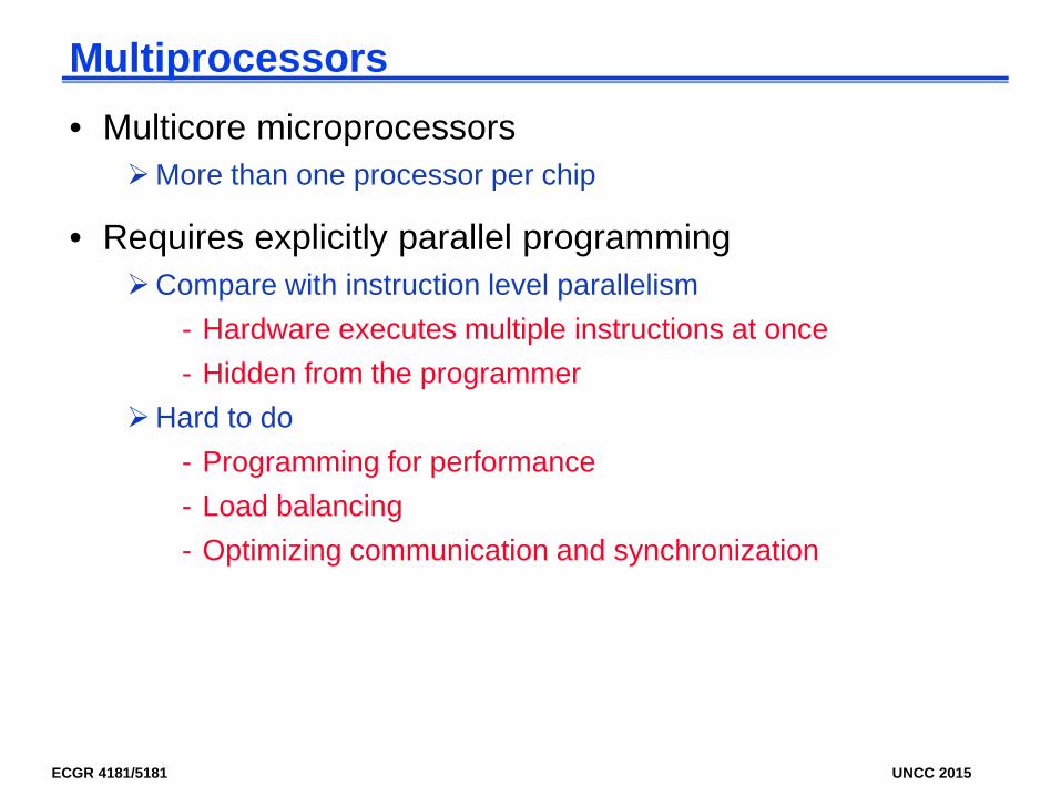
Multiprocessors• Multicore microprocessors
More than one processor per chip
• Requires explicitly parallel programmingCompare with instruction level parallelism
- Hardware executes multiple instructions at once- Hidden from the programmer
Hard to do- Programming for performance- Load balancing- Optimizing communication and synchronization

ECGR 4181/5181 UNCC 2015
Fallacies and Pitfalls
• Fallacy The relative performance of two processors with the same ISA can be judged by clock rate or by the performance of a single benchmark suite.
As processors have become faster and more sophisticated, processor performance in one application area can diverge from that in another area. Sometimes the ISA is responsible, but more often the pipeline structure and memory system are responsible. Thus the clock rate is not a good metric.
Performance of a 1.7 GHz Pentium 4 relative to a 1 GHz Pentium III
ECGR 4181/5181 UNCC 2015
Fallacies and Pitfalls
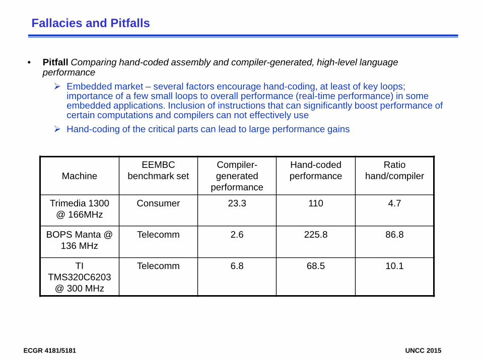
• Pitfall Comparing hand-coded assembly and compiler-generated, high-level language performance Embedded market – several factors encourage hand-coding, at least of key loops;
importance of a few small loops to overall performance (real-time performance) in some embedded applications. Inclusion of instructions that can significantly boost performance of certain computations and compilers can not effectively use
Hand-coding of the critical parts can lead to large performance gains
MachineEEMBC
benchmark setCompiler-generated
performance
Hand-coded performance
Ratio hand/compiler
Trimedia 1300 @ 166MHz
Consumer 23.3 110 4.7
BOPS Manta @ 136 MHz
Telecomm 2.6 225.8 86.8
TI TMS320C6203
@ 300 MHz
Telecomm 6.8 68.5 10.1
ECGR 4181/5181 UNCC 2015
Fallacies and Pitfalls
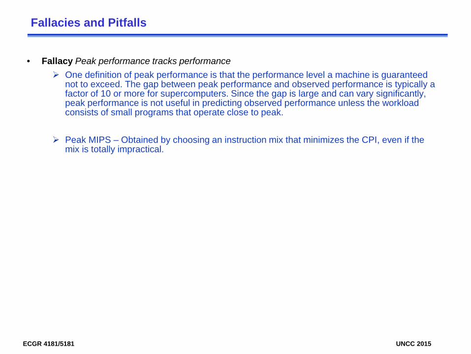
• Fallacy Peak performance tracks performance One definition of peak performance is that the performance level a machine is guaranteed
not to exceed. The gap between peak performance and observed performance is typically a factor of 10 or more for supercomputers. Since the gap is large and can vary significantly, peak performance is not useful in predicting observed performance unless the workload consists of small programs that operate close to peak.
Peak MIPS – Obtained by choosing an instruction mix that minimizes the CPI, even if the mix is totally impractical.
ECGR 4181/5181 UNCC 2015
Fallacies and Pitfalls
• Fallacy The best design for a computer is the one that optimizes the primary objective without considering implementation
Complex designs take longer to complete and prolong time to market – design will be less competitive
• Pitfall Neglecting the cost of software in either evaluating a system or examining cost-performance
For many years, hardware was so expensive that it dominated the cost of software, but this is no longer true
For medium-size database sever the software costs are roughly 50% of the total cost while for desktop the software cost somewhere between 23% and 38%

ECGR 4181/5181 UNCC 2015
Fallacies and Pitfalls
• Pitfall Falling prey to Amdahl’s Law Expending tremendous effort optimizing some aspect of a system before measuring its
usage
• Fallacy MIPS is an accurate measure for comparing performance among processors
Embedded market uses Dhrystone as the benchmark of choice and reports performance as Dhrystone MIPS
Easy to understand Faster machines have higher MIPS rating – matches intuition
6
66
10 MIPSIC timeExecution
10 CPIrateclock
10 imeExection tcountn Instructio MIPS
×=
×=
×=
ECGR 4181/5181 UNCC 2015
Fallacies and Pitfalls
• Problems with using MIPS as a measure for comparison: MIPS is dependent on the instruction set, making it difficult to
compare MIPS of computers with different instruction sets
MIPS varies between programs on the same computer
MIPS can vary inversely to performance. Example: MIPS rating of a machine with optional floating-point hardware. Takes more clock cycles per floating-point instruction than integer instruction – floating-point programs using optional hardware instead software floating-point routines take less time but have a lower MIPS rating. Software floating point executes simpler instructions resulting in higher MIPS rating, but it executes so many instructions that the execution time is longer.
• MIPS is sometimes used by a single vendor within a single set of machines designed for a given class of applications
ECGR 4181/5181 UNCC 2015
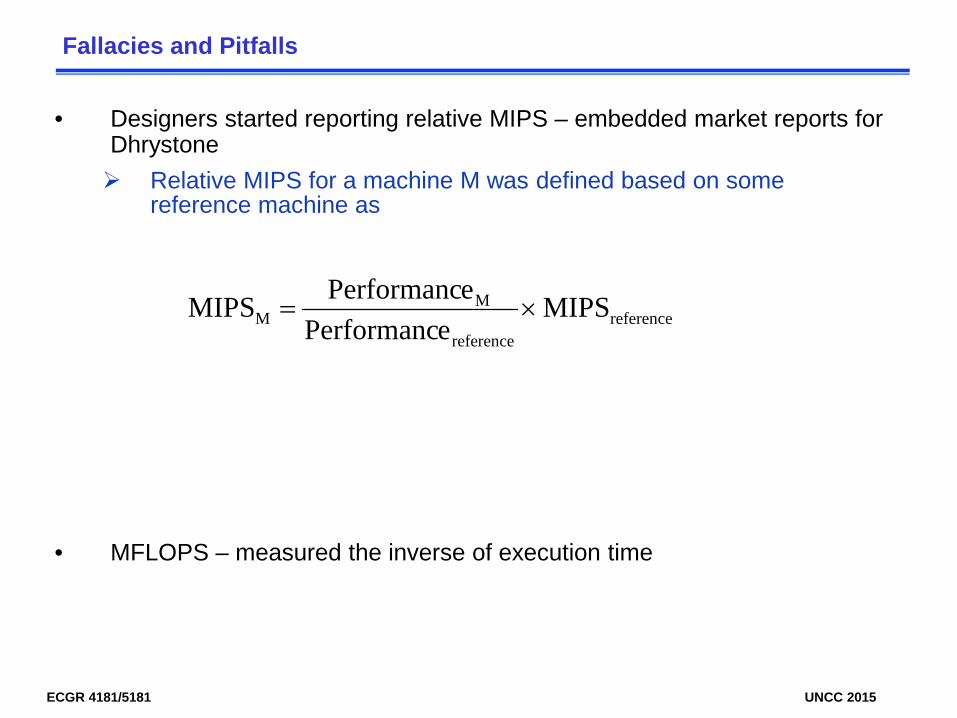
Fallacies and Pitfalls
• Designers started reporting relative MIPS – embedded market reports for Dhrystone Relative MIPS for a machine M was defined based on some
reference machine as
• MFLOPS – measured the inverse of execution time
referencereference
MM MIPS
ePerformancePerformanc MIPS ×=
ECGR 4181/5181 UNCC 2015
Other Performance Metrics
• Power consumption – especially in the embedded market where battery life is important (and passive cooling)For power-limited applications, the most important metric is
energy efficiency

ECGR 4181/5181 UNCC 2015
Summary: Evaluating ISAs• Design-time metrics:
Can it be implemented, in how long, at what cost?Can it be programmed? Ease of compilation?
• Static Metrics:How many bytes does the program occupy in memory?
• Dynamic Metrics:How many instructions are executed? How many bytes does the
processor fetch to execute the program?How many clocks are required per instruction?How "lean" a clock is practical?
Best Metric: Time to execute the program!
CPI
Inst. Count Cycle Timedepends on the instructions set, the processor organization, and compilation techniques.