computer graphics cs 543 lecture 13a curves, tesselation...
TRANSCRIPT

Computer Graphics CS 543 Lecture 13a
Curves, Tesselation/Geometry Shaders & Level of Detail
Prof Emmanuel Agu
Computer Science Dept.
Worcester Polytechnic Institute (WPI)
So Far…
Dealt with straight lines and flat surfaces
Real world objects include curves
Need to develop:
Representations of curves
Tools to render curves
Curve Representation: Explicit
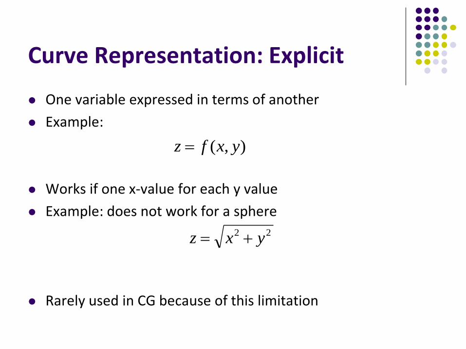
One variable expressed in terms of another
Example:
Works if one x-value for each y value
Example: does not work for a sphere
Rarely used in CG because of this limitation
),( yxfz
22 yxz
Curve Representation: Implicit
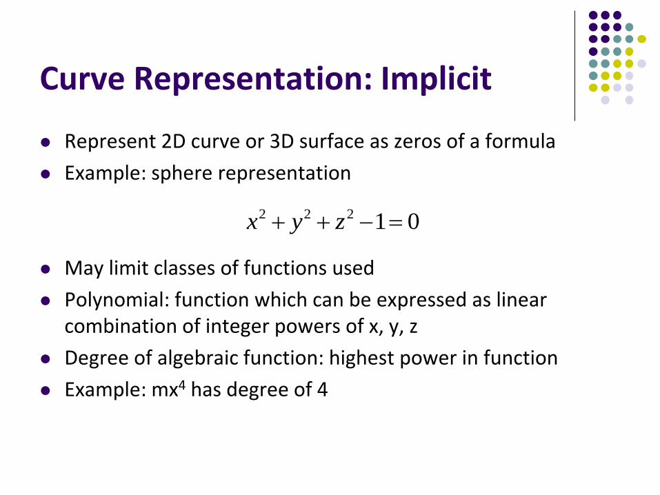
Represent 2D curve or 3D surface as zeros of a formula
Example: sphere representation
May limit classes of functions used
Polynomial: function which can be expressed as linear combination of integer powers of x, y, z
Degree of algebraic function: highest power in function
Example: mx4 has degree of 4
01222 zyx
Curve Representation: Parametric
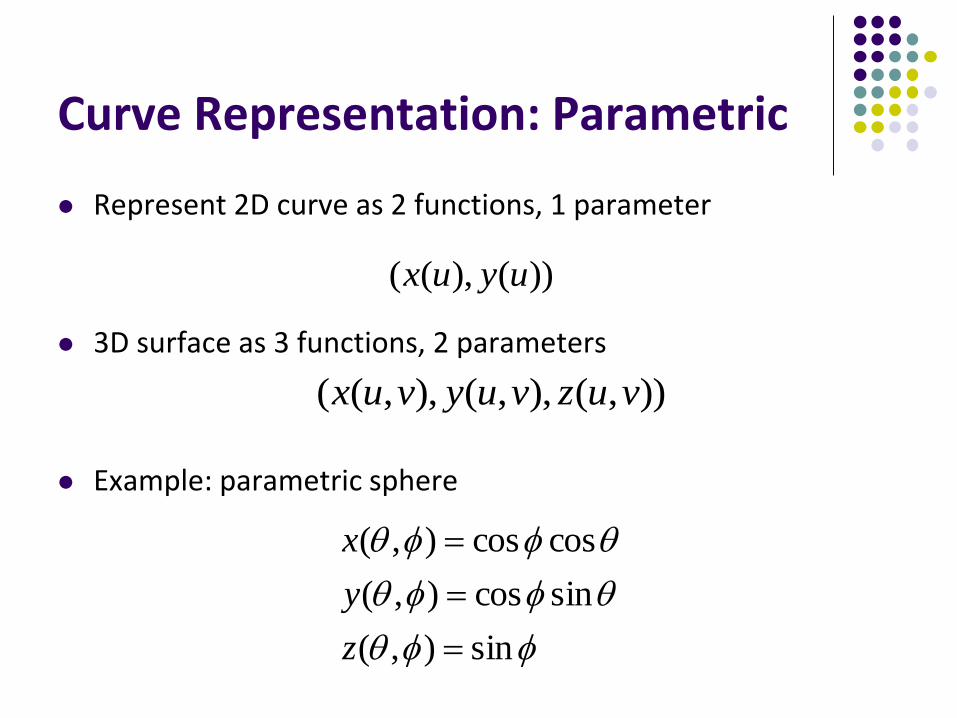
Represent 2D curve as 2 functions, 1 parameter
3D surface as 3 functions, 2 parameters
Example: parametric sphere
))(),(( uyux
)),(),,(),,(( vuzvuyvux
sin),(
sincos),(
coscos),(
z
y
x
Choosing Representations
Different representation suitable for different applications
Implicit representations good for:
Computing ray intersection with surface
Determing if point is inside/outside a surface
Parametric representation good for:
Dividing surface into small polygonal elements for rendering
Subdivide into smaller patches
Sometimes possible to convert one representation into another

Continuity
Consider parametric curve
We would like smoothest curves possible
Mathematically express smoothness as continuity (no jumps)
Defn: if kth derivatives exist, and are continuous, curve has kth order parametric continuity denoted Ck
TuzuyuxuP ))(),(),(()(

Continuity
0th order means curve is continuous
1st order means curve tangent vectors vary continuously, etc

Interactive Curve Design
Mathematical formula unsuitable for designers
Prefer to interactively give sequence of points (control points)
Write procedure:
Input: sequence of points
Output: parametric representation of curve

Interactive Curve Design
1 approach: curves pass through control points (interpolate)
Example: Lagrangian Interpolating Polynomial
Difficulty with this approach: Polynomials always have “wiggles”
For straight lines wiggling is a problem
Our approach: approximate control points (Bezier, B-Splines)called De Casteljau’s algorithm
De Casteljau Algorithm
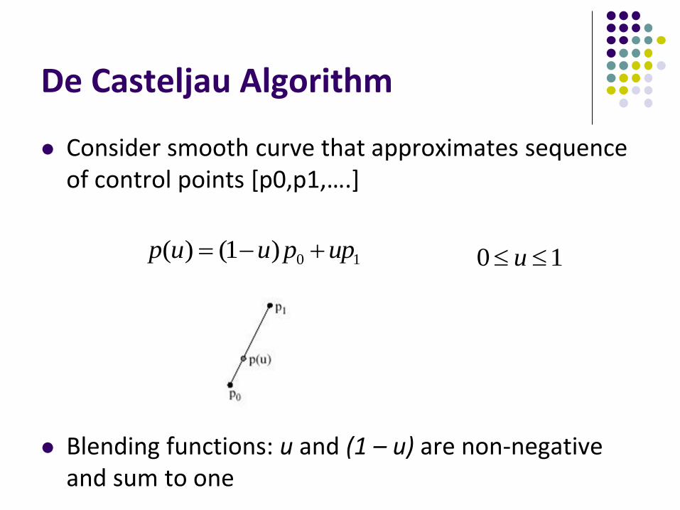
Consider smooth curve that approximates sequence of control points [p0,p1,….]
Blending functions: u and (1 – u) are non-negative and sum to one
10)1()( uppuup 10 u
De Casteljau Algorithm
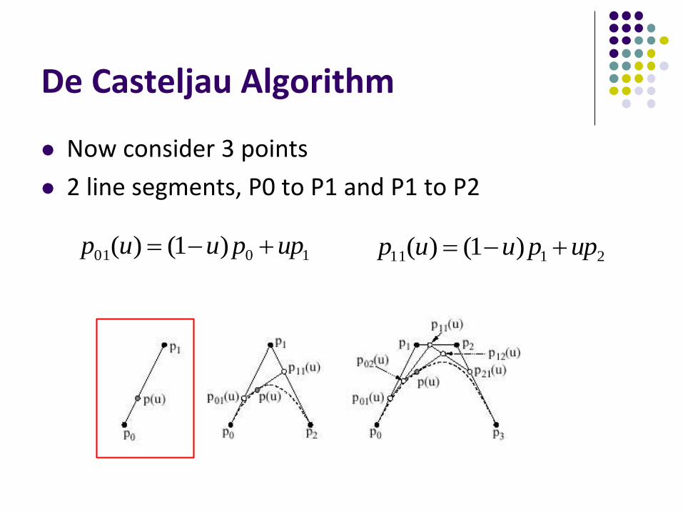
Now consider 3 points
2 line segments, P0 to P1 and P1 to P2
1001 )1()( uppuup 2111 )1()( uppuup

De Casteljau Algorithm
)()1()( 1101 uuppuup
2
2
10
2 ))1(2()1( pupuupu
2
02 )1()( uub
Blending functions for degree 2 Bezier curve
)1(2)(12 uuub 2
22 )( uub
)(02 ub )(12 ub )(22 ub
Substituting known values of and )(01 up )(11 up
Note: blending functions, non-negative, sum to 1

De Casteljau Algorithm
Extend to 4 control points P0, P1, P2, P3
Final result above is Bezier curve of degree 3
3
2
2
1
2
0
3 ))1(3())1(3()1()( upuupuupuup
)(23 ub)(03 ub )(13 ub )(33 ub
De Casteljau Algorithm
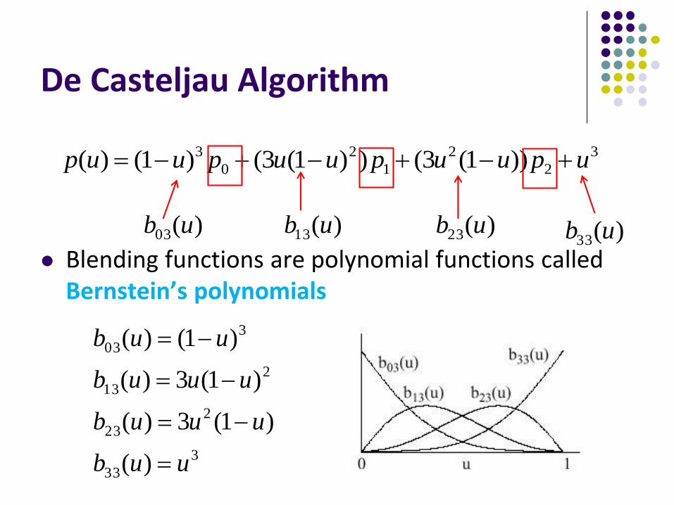
Blending functions are polynomial functions called Bernstein’s polynomials
3
33
2
23
2
13
3
03
)(
)1(3)(
)1(3)(
)1()(
uub
uuub
uuub
uub
3
2
2
1
2
0
3 ))1(3())1(3()1()( upuupuupuup
)(23 ub)(03 ub )(13 ub )(33 ub

De Casteljau Algorithm
Writing coefficient of blending functions gives Pascal’s triangle
1
4
1
1
1
1
1
2
4
3
6
1 3
1
1
3
2
2
1
2
0
3 ))1(3())1(3()1()( upuupuupuup
31 3 1
4 control points
3 control points
5 control points

De Casteljau Algorithm
In general, blending function for k Bezier curve has form
Example
iik
ik uui
kub
)1()(
3003
03 )1()1(0
3)( uuuub
De Casteljau Algorithm
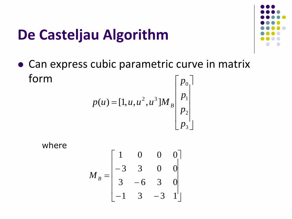
Can express cubic parametric curve in matrix form
3
2
1
0
32 ],,,1[)(
p
p
p
p
Muuuup B
where
1331
0363
0033
0001
BM
Subdividing Bezier Curves
OpenGL renders flat objects
To render curves, approximate with small linear segments
Subdivide surface to polygonal patches
Bezier curves useful for elegant, recursive subdivision

Subdividing Bezier Curves
Let (P0… P3) denote original sequence of control points
Recursively interpolate with u = ½ as below
Sequences (P00,P01,P02,P03) and (P03,P12,P21,30) define Bezier curves also
Bezier Curves can either be straightened or curved recursively in this way
Bezier Surfaces
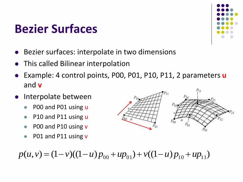
Bezier surfaces: interpolate in two dimensions
This called Bilinear interpolation
Example: 4 control points, P00, P01, P10, P11, 2 parameters uand v
Interpolate between P00 and P01 using u
P10 and P11 using u
P00 and P10 using v
P01 and P11 using v
))1(())1)((1(),( 11100100 uppuvuppuvvup

Bezier Surfaces
Expressing in terms of blending functions
11111101011101000101 )()()()()()(),( pubvbpubbvbpubvbvup
Generalizing
3
0
3
0
,3,3, )()(),(i j
jiji pubvbvup
Problems with Bezier Curves
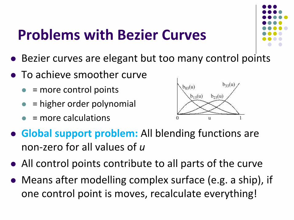
Bezier curves are elegant but too many control points
To achieve smoother curve
= more control points
= higher order polynomial
= more calculations
Global support problem: All blending functions are non-zero for all values of u
All control points contribute to all parts of the curve
Means after modelling complex surface (e.g. a ship), if one control point is moves, recalculate everything!
B-Splines
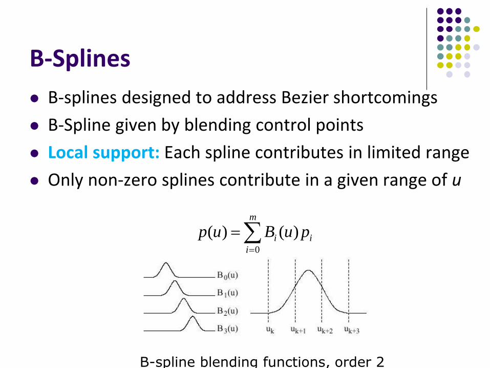
B-splines designed to address Bezier shortcomings
B-Spline given by blending control points
Local support: Each spline contributes in limited range
Only non-zero splines contribute in a given range of u
m
i
ii puBup0
)()(
B-spline blending functions, order 2

NURBS
Encompasses both Bezier curves/surfaces and B-splines
Non-uniform Rational B-splines (NURBS)
Rational function is ratio of two polynomials
Some curves can be expressed as rational functions but not as simple polynomials
No known exact polynomial for circle
Rational parametrization of unit circle on xy-plane:
0)(
1
2)(
1
1)(
2
2
2
uz
u
uuy
u
uux

NURBS
We can apply homogeneous coordinates to bring in w
Useful property of NURBS: preserved under transformation E.g. Rotate sphere defined as NURBS, still a sphere
2
2
1)(
0)(
2)(
1)(
uuw
uz
uuy
uux
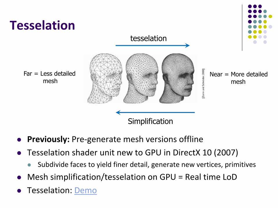
Tesselation
Previously: Pre-generate mesh versions offline
Tesselation shader unit new to GPU in DirectX 10 (2007) Subdivide faces to yield finer detail, generate new vertices, primitives
Mesh simplification/tesselation on GPU = Real time LoD
Tesselation: Demo
tesselation
Simplification
Far = Less detailed mesh
Near = More detailed mesh

Tessellation Shaders
Can subdivide curves, surfaces on the GPU
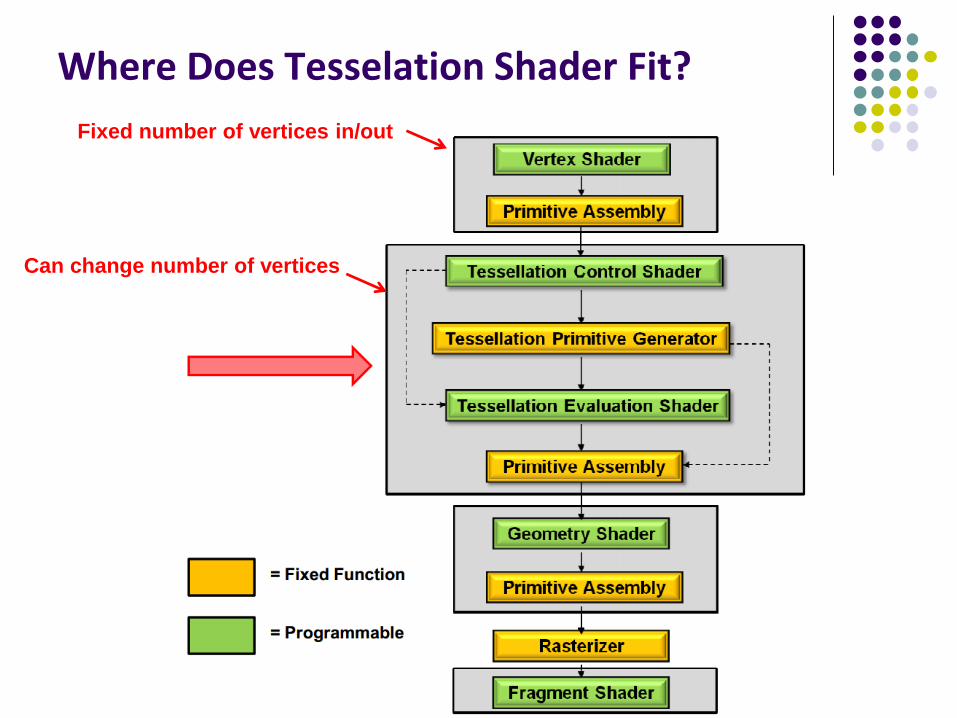
Where Does Tesselation Shader Fit?
Fixed number of vertices in/out
Can change number of vertices
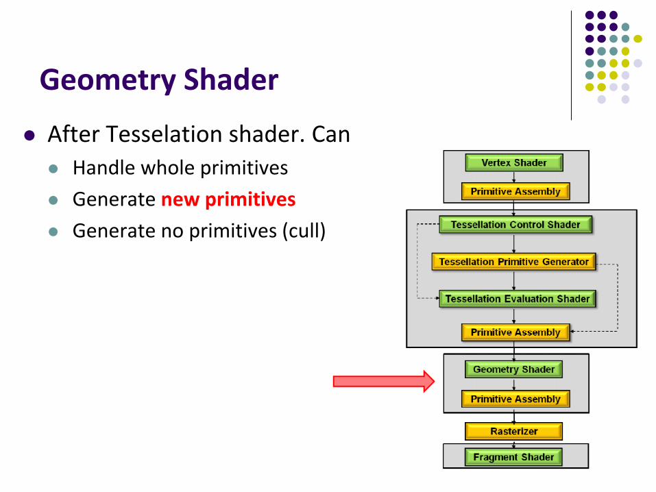
Geometry Shader
After Tesselation shader. Can
Handle whole primitives
Generate new primitives
Generate no primitives (cull)

Level of Detail
Use simpler versions of objects if they make smaller contributions to the image
LOD algorithms have three parts:
Generation: Models of different details are generated
Selection: Chooses which model should be used depending on criteria
Switching: Changing from one model to another
Can be used for models, textures, shading and more

Level of Detail

LOD Switching
Discrete Geometry LODs
LOD is switched suddenly from one frame to the next
Blend LODs
Two LODs are blended together over time
New LOD is faded by increasing alpha value from 0 to 1
More expensive than rendering one LOD
Faded LODs are drawn last to avoid distant objects drawing over the faded LOD

LOD Switching (cont.)
Alpha LOD
Alpha value of object is lowered as distance increases
Experience is more continuous
Performance is only felt when object disappears
Requires sorting of scene based on transparency

LOD Selection
Determining which LOD to render and which to blend
Range-Based:
LOD choice based on distance

Time-Critical LOD Rendering
Using LOD to ensure constant frame rates
Predictive algorithm
Selects the LOD based on which objects are visible
Heuristics:
Maximize
Constraint:
References
Hill and Kelley, chapter 11
Angel and Shreiner, Interactive Computer Graphics, 6th edition, Chapter 10
Shreiner, OpenGL Programming Guide, 8th edition