computersandmathematicswithapplications … ·...
TRANSCRIPT

Computers and Mathematics with Applications 63 (2012) 912–942
Contents lists available at SciVerse ScienceDirect
Computers and Mathematics with Applications
journal homepage: www.elsevier.com/locate/camwa
Comparison of multi-objective optimization methodologies forengineering applicationsG. Chiandussi a, M. Codegone b,∗, S. Ferrero c, F.E. Varesio a
a Politecnico di Torino, Department of Mechanical Engineering, Corso Duca degli Abruzzi 24, 10129 Torino, Italyb Politecnico di Torino, Department of Mathematics, Corso Duca degli Abruzzi 24, 10129 Torino, Italyc Nova Analysis s.n.c., Via Biella 72, 10098 Rivoli (TO), Italy
a r t i c l e i n f o
Article history:Received 29 June 2011Received in revised form 3 November 2011Accepted 30 November 2011
Keywords:Multi-objective optimizationPareto frontMethod effectivenessFinite element methodStructural engineering
a b s t r a c t
Computational models describing the behavior of complex physical systems are oftenused in the engineering design field to identify better or optimal solutions with respectto previously defined performance criteria. Multi-objective optimization problems ariseand the set of optimal compromise solutions (Pareto front) has to be identified by aneffective and complete search procedure in order to let the decision maker, the designer,to carry out the best choice. Four multi-objective optimization techniques are analyzedby describing their formulation, advantages and disadvantages. The effectiveness ofthe selected techniques for engineering design purposes is verified by comparing theresults obtained by solving a few benchmarks and a real structural engineering problemconcerning an engine bracket of a car.
© 2011 Elsevier Ltd. All rights reserved.
1. Introduction
Computational models are commonly used in engineering design activities for the simulation of complex physicalsystems. They are often employed as virtual prototypeswhere a set of predefined systemparameters are adjusted to improveor optimize the performance of the physical system as defined by one or more system performance objectives.
The optimization of a specific virtual prototype requires the implementation of the corresponding computational model,the evaluation of the performance objectives and the iterative adjustment of the system parameters in order to obtain anoptimal solution. Multi-objective optimization problems arise in a natural fashion in the engineering field. It should bepreferable to optimize the objective functions all at once but, in general, they are in competition with each other and theoptimization process has to search for the best optimal compromise solution.
The primary goals in multi-objective optimization problem solution are:
to preserve non dominated points in the objective space and associated solution points in the decision space; to keep making algorithmic progress toward the Pareto front in the objective function space; to maintain diversity of points on the Pareto front and of Pareto optimal solutions (decision space); to provide the decision maker, the designer, with a large enough but limited number of Pareto points for selection.
A preliminary review on single-objective optimization problems is required if the task of a multi-objective optimizationproblem and its attainment has to be fully understood. As a consequence the paper is organized as follows. At first, the basicterminology and nomenclature for use throughout the paper is introduced. Then, a classification of some mathematical
∗ Corresponding author. Tel.: +39 0110907507; fax: +39 0907599.E-mail address:[email protected] (M. Codegone).
0898-1221/$ – see front matter© 2011 Elsevier Ltd. All rights reserved.doi:10.1016/j.camwa.2011.11.057
G. Chiandussi et al. / Computers and Mathematics with Applications 63 (2012) 912–942 913
programming techniques that have been proposed to solve multi-objective optimization problems and the analysis of someof themwill be presented in order to underline their advantages and disadvantages. The results obtained by solving severalbenchmark problems will be shown for comparison purposes. Finally, the results obtained by the study of a real worldengineering design problem concerning an engine bracket will be presented.
1.1. The single-objective optimization problem
A single-objective optimization problem can be defined as:
Definition 1 (General Single-Objective Optimization Problem). A general single-objective optimization problem is defined asthe minimization (or maximization) of a scalar objective function f (x) subject to inequality constraints gi(x) ≤ 0, i =
1, . . . ,m and equality constraints hj (x) = 0, j = 1, . . . , p where x is a n-dimensional decision variable vectorx = (x1, . . . , xn) from some universe Ω . Ω contains all possible x that can be used to satisfy an evaluation of f (x) andits constraints. Of course, x can be a vector of continuous or discrete variables as well as f being continuous or discrete.
Observe that gi(x) ≤ 0 and hj(x) = 0 represent constraints that must be fulfilled while optimizing (minimizing ormaximizing) f (x). Constraints can be explicit (i.e., given in algebraic form) or implicit, inwhich case the algorithm to computegi(x) for any given vector xmust be known. Note that p, the number of independent equality constraints, must be less thann, the number of decision variables, because if p ≥ n the problem is said to be over-constrained since there are no degrees offreedom left for optimizing (i.e., in other words, there would be more equations than unknowns). The number of degrees offreedom is given by n−p if the equality constraints are independent and the inequality constraints do not reduce to equalityconstraints.
The method for finding the global optimum of any function (may not be unique) is referred to as Global Optimization. Ingeneral, the global minimum of a single-objective problem is presented in Definition 2 [1]:
Definition 2 (Single-Objective Global Minimum Optimization). Given a function f : Ω ⊆ Rn→ R, Ω = ∅, for x ∈ Ω the
value f ∗ , f (x∗) > −∞ is called a global minimum if and only if:
∀x ∈ Ω : fx∗
≤ f (x) (1.1)
where x∗ is by definition the globalminimum solution, f is the objective function and the setΩ is the feasible region of x. Thegoal of determining the global minimum solution is called the global optimization problem for a single-objective problem.
1.2. The multi-objective optimization problem
Multi-objective problems are those problems where the goal is to optimize simultaneously k objective functionsdesignated as: f1 (x) , f2 (x) , . . . , fk (x) and forming a vector function F(x):
F (x) =
f1(x)f2(x)
...fk(x)
. (1.2)
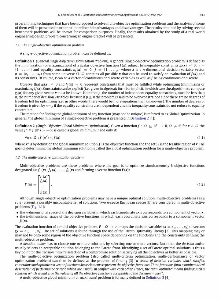
Although single-objective optimization problems may have a unique optimal solution, multi-objective problems (as arule) present a possibly uncountable set of solutions. Two n-space Euclidean spaces Rn are considered in multi-objectiveproblems (Fig. 1.1):• the n-dimensional space of the decision variables in which each coordinate axis corresponds to a component of vector x;• the k-dimensional space of the objective functions in which each coordinate axis corresponds to a component vector
fk(x).
The evaluation function of a multi-objective problem, F : Ω → Λ, maps the decision variables (x = x1, . . . , xn) to vectors(y = a1, . . . , ak). The set of solutions is found through the use of the Pareto Optimality Theory [2]. This mapping may ormay not be onto some region of the objective function space depending on the functions and the constraints defining themulti-objective problem.
A decision maker has to choose one or more solutions by selecting one or more vectors. Note that the decision makerusually selects an acceptable solution belonging to the Pareto front. Identifying a set of Pareto optimal solutions is thus akey point for the decision maker ’s selection of a compromise solution satisfying all the objectives as better as possible.
The multi-objective optimization problem (also called multi-criteria optimization, multi-performance or vectoroptimization problem) can then be defined as the problem of finding [3] ‘‘a vector of decision variables which satisfiesconstraints and optimizes a vector functionwhose elements represent the objective functions. These functions form amathematicaldescription of performance criteria which are usually in conflict with each other. Hence, the term ‘optimize’ means finding such asolution which would give the values of all the objective functions acceptable to the decision maker ’’.
A multi-objective global minimum (or maximum) problem is formally defined in Definition 3 [4]:
914 G. Chiandussi et al. / Computers and Mathematics with Applications 63 (2012) 912–942
Fig. 1.1. Evaluation mapping of a multi-objective problem.
Definition 3 (General Multi-Objective Optimization Problem). A general multi-objective optimization problem is defined asthe minimization (or maximization) of the objective function set F(x) = ( f1(x), . . . , fk(x)) subject to inequality constraintsgi(x) ≤ 0, i = 1, . . . ,m, and equality constraints hj(x) = 0, j = 1, . . . , p. The solution of a multi-objectiveproblem minimizes (or maximizes) the components of a vector F(x) where x is a n-dimensional decision variable vectorx = (x1, . . . , xn) from some universe Ω . It is noted that gi(x) ≤ 0 and hj(x) = 0 represent constraints that must be fulfilledwhile minimizing (or maximizing) F(x) and Ω contains all possible x that can be used to satisfy an evaluation of F(x).
Thus, a multi-objective problem consists of k objectives reflected in the k objective functions, m + p constraints on theobjective functions and n decision variables. The k objective functions may be linear or nonlinear and continuous or discretein nature. Of course, the vector of decision variables xi can also be continuous or discrete.
Definition 4 (Ideal Vector). Let:
x0(i) =
x0(i)1 , x0(i)2 , . . . , x0(i)n
T(1.3)
be a vector of variables which optimizes (either minimizes or maximizes) the ith objective function fi(x). In other words, thevector x0(i) ∈ Ω is such that:
fix0(i)
= opt fi(x). (1.4)
Then, the vector:
f0 =f 01 , f 02 , . . . , f 0k
T(1.5)
where f 0i denotes the optimum of the ith function, is ideal for an multi-objective problem and the point in Rn whichdetermined this vector is the ideal solution and is consequently called the ideal vector. In other words, the ideal vectorcontains the optimum for each separately considered objective achieved at the same point in Rn.
Definition 5 (Convexity). A function φ(x) is called convex over the domain of R if for any two vectors x1 and x2 ∈ R:
φ (θx1 + (1 − θ)x2) ≤ θφ (x1) + (1 − θ)φ(x2) (1.6)
where θ is a scalar in the range 0 ≤ θ ≤ 1. A convex function cannot have any value larger than the function values obtainedby linear interpolation between φ (x1) and φ(x2). If the reverse inequality of the previous equation holds, the function isconcave. Thus φ(x) is concave if −φ(x) is convex. Linear functions are convex and concave at the same time.
A set of points (or region) is defined as a convex set in n-dimensional space if, for all pairs of two points x1 and x2 in theset, the straight-line segment joining them is also entirely in the set. Thus, every point x, where:
x = θx1 + (1 − θ) x2 0 ≤ θ ≤ 1 (1.7)
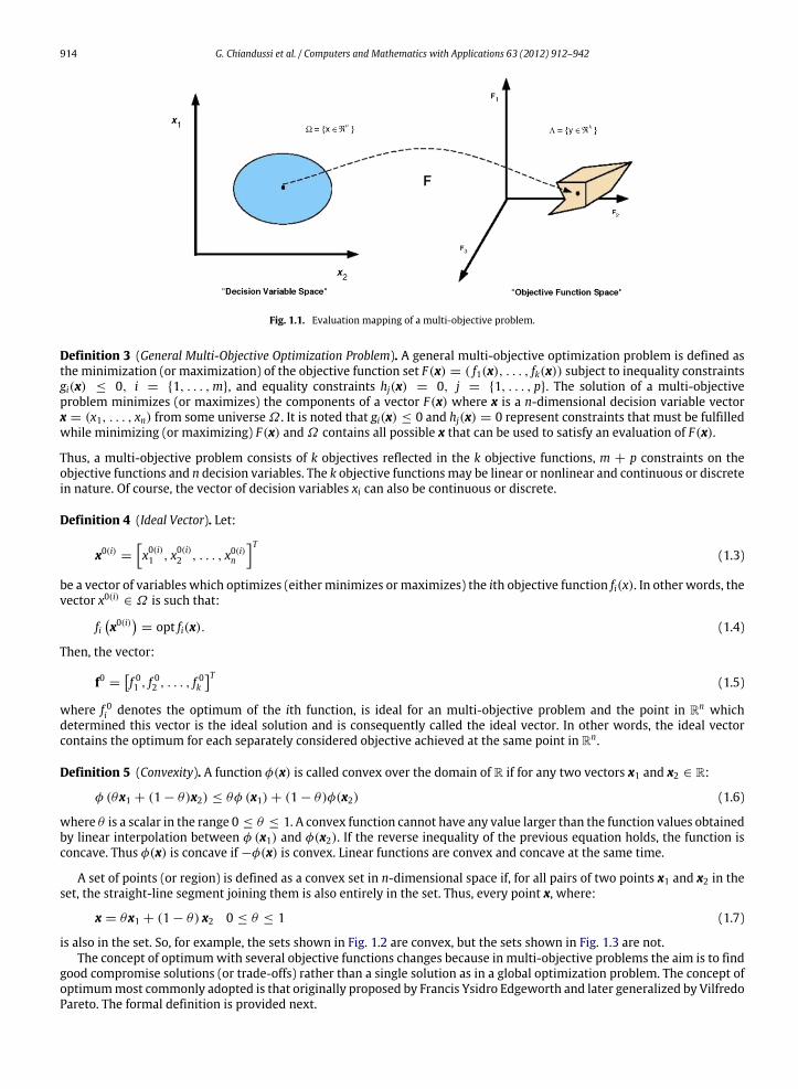
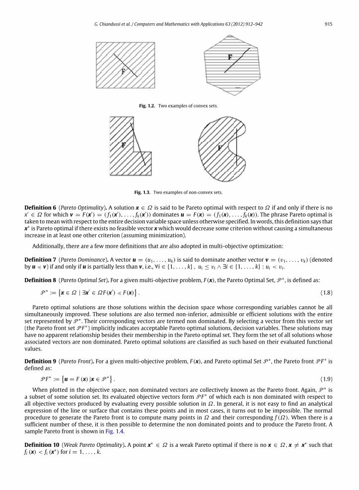
is also in the set. So, for example, the sets shown in Fig. 1.2 are convex, but the sets shown in Fig. 1.3 are not.The concept of optimumwith several objective functions changes because in multi-objective problems the aim is to find
good compromise solutions (or trade-offs) rather than a single solution as in a global optimization problem. The concept ofoptimummost commonly adopted is that originally proposed by Francis Ysidro Edgeworth and later generalized by VilfredoPareto. The formal definition is provided next.
G. Chiandussi et al. / Computers and Mathematics with Applications 63 (2012) 912–942 915
Fig. 1.2. Two examples of convex sets.
Fig. 1.3. Two examples of non-convex sets.
Definition 6 (Pareto Optimality). A solution x ∈ Ω is said to be Pareto optimal with respect to Ω if and only if there is nox′
∈ Ω for which v = F(x′) = ( f1(x′), . . . , fk(x′)) dominates u = F(x) = ( f1(x), . . . , fk(x)). The phrase Pareto optimal istaken tomeanwith respect to the entire decision variable space unless otherwise specified. Inwords, this definition says thatx∗ is Pareto optimal if there exists no feasible vector xwhichwould decrease some criterionwithout causing a simultaneousincrease in at least one other criterion (assuming minimization).
Additionally, there are a few more definitions that are also adopted in multi-objective optimization:
Definition 7 (Pareto Dominance). A vector u = (u1, . . . , uk) is said to dominate another vector v = (v1, . . . , vk) (denotedby u 4 v) if and only if u is partially less than v, i.e., ∀i ∈ 1, . . . , k , ui ≤ vi ∧ ∃i ∈ 1, . . . , k : ui < vi.
Definition 8 (Pareto Optimal Set). For a given multi-objective problem, F(x), the Pareto Optimal Set, P ∗, is defined as:
P ∗:=x ∈ Ω | ∃x′
∈ ΩF(x′) 4 F(x). (1.8)
Pareto optimal solutions are those solutions within the decision space whose corresponding variables cannot be allsimultaneously improved. These solutions are also termed non-inferior, admissible or efficient solutions with the entireset represented by P ∗. Their corresponding vectors are termed non dominated. By selecting a vector from this vector set(the Pareto front set P F∗) implicitly indicates acceptable Pareto optimal solutions, decision variables. These solutions mayhave no apparent relationship besides their membership in the Pareto optimal set. They form the set of all solutions whoseassociated vectors are non dominated. Pareto optimal solutions are classified as such based on their evaluated functionalvalues.
Definition 9 (Pareto Front). For a given multi-objective problem, F(x), and Pareto optimal Set P ∗, the Pareto front P F∗ isdefined as:
P F∗:=u = F (x) |x ∈ P ∗
. (1.9)
When plotted in the objective space, non dominated vectors are collectively known as the Pareto front. Again, P ∗ isa subset of some solution set. Its evaluated objective vectors form P F∗ of which each is non dominated with respect toall objective vectors produced by evaluating every possible solution in Ω . In general, it is not easy to find an analyticalexpression of the line or surface that contains these points and in most cases, it turns out to be impossible. The normalprocedure to generate the Pareto front is to compute many points in Ω and their corresponding f (Ω). When there is asufficient number of these, it is then possible to determine the non dominated points and to produce the Pareto front. Asample Pareto front is shown in Fig. 1.4.
Definition 10 (Weak Pareto Optimality). A point x∗∈ Ω is a weak Pareto optimal if there is no x ∈ Ω, x = x∗ such that
fi (x) < fi (x∗) for i = 1, . . . , k.

916 G. Chiandussi et al. / Computers and Mathematics with Applications 63 (2012) 912–942
Fig. 1.4. Pareto front of a problem with two objective functions: cost and efficiency.
Definition 11 (Strict Pareto Optimality). A point x∗∈ Ω is a strictly Pareto optimal if there is no x ∈ Ω, x = x∗ such that
fi (x) ≤ fi (x∗) for i = 1, . . . , k.
Definition 12 (Kuhn–Tucker Conditions for Non Inferiority). If a solution x to the general multi-objective problem is noninferior, then there exist wl = 0, l = 1, 2, . . . , k (wr is strictly positive for some r = 1, 2, . . . , k), and λi = 0, i =
1, 2, . . . ,m, such that:
x ∈ Ω (1.10)
and:
kl=1
wl∇fl (x) −
mi=1
λi∇gi (x) = 0. (1.11)
These conditions are necessary for a non inferior solution and, when all of the fl(x) are concave and Ω is a convex set, theyare sufficient as well.
Pareto optimal solutions are those which, when evaluated, produce vectors whose performance fi cannot be improvedwithout adversely affecting another fj, i = j. The Pareto front P F∗ determined by evaluating P ∗ is fixed by the definedmulti-objective problem and does not change. Thus, P ∗ represents the best solutions available and allows the definition ofthe global optimum of a multi-objective problem.
Definition 13 (Multi-Objective Global Minimum). Given a function f : Ω ⊆ Rn→ Rk, Ω = ∅, k > 2, for x ∈ Ω the set
P F∗ , fx∗
i
> (−∞, . . . ,−∞) is called the global minimum if and only if:
∀x ∈ Ω : fx∗
i
4 f (x) . (1.12)
Then, x∗
i , i = 1, . . . , n is the global minimum solution set (i.e., P ∗), f is the multiple objective function, and the set Ω
is the feasible region. The problem of determining the global minimum solution set is called the multi-objective globaloptimization problem.
2. Multi-objective optimization techniques
There have been several attempts to classify themulti-objective optimization techniques currently in use. First of all, it isquite important to distinguish the two stages inwhich the solution of amulti-objective optimization problemcanbedivided:the optimization of the objective functions involved and the process of decidingwhat kind of trade-offs are appropriate fromthe decision maker perspective (the so-called multi-criteria decision making process). In this section, some of the manytechniques available for these two stages are discussed by analyzing some of their advantages and disadvantages.
Cohon and Marks [5] proposed one of the most popular classification of techniques within the Operations Researchcommunity that focuses on the way in which each method handles the two problems of searching and making decisions:
G. Chiandussi et al. / Computers and Mathematics with Applications 63 (2012) 912–942 917
1. a priori Preference Articulation: take decisions before searching (decide ⇒ search). This group of techniques includesthose approaches that assume that either a certain desired achievable goals or a certain pre-ordering of the objectivescan be performed by the decision maker prior to the search.
2. a posteriori Preference Articulation: search before making decisions (search ⇒ decide). These techniques do not requireprior preference information from the decision maker. Some of the techniques included in this category are among theoldest multi-objective optimization approaches proposed.
3. Progressive Preference Articulation: integrate search and decisionmaking (decide⇔ search). These techniques normallyoperate in three stages: find a non dominated solution, get the reaction of the decision maker regarding this non dominated solution and modify the preferences of the
objectives accordingly, repeat the two previous steps until the decision maker is satisfied or no further improvement is possible.
A different kind of approach is represented by Evolutionary Algorithms that are based on Darwin’s theory of survival ofthe fittest. They are found on the idea that as the population evolves in a genetic algorithm, solutions that are non-dominatedare chosen to remain in the population.
One a priori Preference Articulation, two a posteriori Preference Articulations and one Evolutionary Algorithm have beenanalyzed and compared in terms of performance in the following sections.
2.1. Global criterion method
The global criterionmethod is an a priori Preference Articulation. Its aim is tominimize a function (global criterion)whichis a measure of how close the decision maker can get to the ideal vector f 0. The most common form of this function is [6]:
f (x) =
ki=1
f 0i − fi(x)
f 0i
p
(1.13)
where k is the number of objectives. For this formula Boychuk and Ovchinnikov [7] have suggested the exponent p = 1whereas Salukvadze [8] has suggested p = 2, but other values of p can also be used. Obviously, the results differ greatlydepending on the value of the exponent p chosen. Thus, the selection of the best p is an issue in this method and it couldalso be the case that any p could produce an unacceptable solution.
Another possible measure of closeness to the ideal solution is a family of Lp-metrics defined as follows:
Lp(f ) =
k
i=1
f 0i − fi(x)p1/p
, 1 ≤ p ≤ ∞. (1.14)
In general, relative deviations of the form:
f 0i − fi(x)f 0i
(1.15)
are preferred over absolute deviations because they have a substantive meaning in any context. The relevant Lp metrics are:
Lp(f ) =
k
i=1
f 0i − fi(x)f 0i
p1/p
, 1 ≤ p ≤ ∞. (1.16)
The value of p points out the type of distance. For p = 1, all deviations from f ∗
i are taken into account in direct proportion totheir magnitudes which corresponds to ‘group utility’. For 2 ≤ p < ∞, the larger deviations carry greater weight in Lp. Forp = ∞, the largest deviation is the only one taken into consideration which leads to a purely ‘individual utility’ (min–maxcriterion) in which all weighted deviations are equal.
Koski [9] has suggested Lp-metrics with a normalized vector objective function of the form:
fi (x) =
fi (x) − minx∈F
fi(x)
maxx∈F
fi (x) − minx∈F
fi (x). (1.17)
In this case, the values of every normalized function are limited to the range [0, 1].Using the global criterion method one non-inferior solution is obtained. If certain parameters wi are used as weights for
the criteria, a required set of non-inferior solutions can be found. Duckstein [10] calls thismethod compromise programmingand his Lp-metric is:
Lp (x) =
k
i=1
wpi
fi (x) − f 0ifi max − f 0i
p1/p
(1.18)

918 G. Chiandussi et al. / Computers and Mathematics with Applications 63 (2012) 912–942
where wi are the weights, fi max is the worst value obtainable for criterion i, fi(x) is the result of implementing decision xwith respect to the ith criterion. The displaced ideal technique which proceeds to define an ideal point, a solution point,another ideal point, etc. is an extension of compromise programming.
Another variation of this technique is the method suggested by Wierzbicki [11] in which the global function has aform that penalizes the deviations from the so-called reference objective. Any reasonable or desirable point in the spaceof objectives chosen by the decision maker can be considered as the reference objective. Let fT =
f r1 , f r2 , . . . , f rk
T be avector which defines this point. Then the function which is minimized has the form:
Px, fT
= −
ki=1
(fi(x) − f ri )2 + ϱ
ki=1
max(0, (fi(x) − f ri )2) (1.19)
where ϱ > 0 is a penalty coefficient which in this method can be chosen as constant. Minimizing (1.19) for the assumedpoint fr a non-inferior solution which is close to this point can be obtained. If for different points fr the procedure is carriedout, some representation of non-inferior solutions can be found.
The main advantage of these methods is their simplicity and their effectiveness because they do not require a Paretoranking procedure. However, their main disadvantage is the definition of the desired goals which requires some extracomputational effort. An additional problem with these techniques is that they will yield a non dominated solution onlyif the goals are chosen in the feasible domain and such conditions may certainly limit their applicability. More informationon these methods can be found in [6,12,13].
2.2. Linear combination of weights
Zadeh [14] was the first to show that the third of the Kuhn–Tucker conditions for non inferior solutions implies that noninferior solutions might be found by solving a scalar optimization problem in which the objective function is a weightedsum of the components of the original vector-valued function. That is, the solution to the following problem:
mink
i=1
αifi(x) (1.20)
subject to:
x ∈ Ω (1.21)
where αi ≥ 0 for all i and strictly positive for at least one objective, is usually non inferior. The non inferior set and the set ofnon inferior solutions can be generated by parametrically varying the weights αi in the objective function. This was initiallydemonstrated by Gass and Saaty [15] for a two-objective problem.
The reduction of the problem to a single-objective functionmeans tomake all alternatives comparable with a preferenceframework that becomes a total order. Hence αi values choice is very important to achieve the final decision and, for thisreason, value choice is made by the decision maker. However the decision maker, in order to choose the coefficients, musthave a clear perception of how this choice influence optimal points.
Let consider a particular solution x for which the value of the objective function is fi = fi(x). Let fix two criteria h and kand a value ∆h > 0 little enough. The decision maker is asked for which value ∆k > 0 there is no difference among x and anhypothetical alternative that gives values f ∗
i = fi for i = h, k and fh = fh −∆h and fk = fk +∆k. It is reasonable to think thatsuch value ∆h > 0 exists. Indeed for ∆h > 0 the hypothetical alternative dominates x while increasing ∆k the situation isexpected to be reversed. Because of the indifference of the two alternatives, the following must hold:
i
αifi =
i
αif ∗
i ⇒ 0 = αk∆k − αh∆h ⇒αh
αk=
∆k
∆h. (1.22)
The previous equation links the coefficients of the linear combination to the comparative evaluation among the two criteria.Varying h on all criteria, αh can be described through αk. Since coefficients are defined up to a positive constant (indeedmultiply all for the same positive constant does not change the problem (1.20)), αk can be set as αk = 1 and so αh = ∆k/∆h.Obviously the bigger is the coefficient αh, the more the objective h is taken into account in the decision choice. Moreover ithas no meaning to consider a coefficient equal to zero since it would say non considering the corresponding objectives.
The procedure described implicitly assumed the linearity of the objective functions. In other words the values ∆h candepend on levels fh of the objective considered. If the h criterion has been satisfied yet, the decision maker could prefer toimprove further while it could take an opposite behavior for a non-satisfying level. The interaction with the decision makernormally supposes of resolving several times the problem (1.20) attempting different values for αi until a satisfying solutionis found.
The positive aspect of this approach is that min F(x) : x ∈ X provides a Pareto optimal point. Indeed if y is a dominatedsolution by x, from dominance definition the following holds:
αifi(x) ≤ αifi(y) with i = 1, . . . ,m and αkfk(x) < αkfk(y) (1.23)

G. Chiandussi et al. / Computers and Mathematics with Applications 63 (2012) 912–942 919
Fig. 2.1. The weighted sum method fails for non-convex problems.
leading to:i
αifi(x) <
i
αifi(y). (1.24)
Thus no dominated solution can be optimum of (1.20).On the contrary, a negative aspect is due to the fact that is usually not true that each Pareto optimal can be obtained
through a suitable choice of αi coefficients. The reason is the following: to solve (1.20) is equivalent to minimize the linearfunctional
i αiyi for y ∈ f (X). A minimum of a linear functional on a set Y belongs both to the set Y and to the border of
the convex envelope of Y . Hence, those non dominated points that do not lie on the border of the convex envelope cannot begenerated by (1.20).More exactly, since only positiveαi coefficients are admitted, solving (1.20) generates only solutions thatlie on the border of the convex envelope f (X) + Rm
+. In order to explain these concepts, let consider the following example:
let X =x ∈ R2
: x21 + x22 = 1and f (x) = x; in this case the efficient point set being XE =
x ∈ R2
: x21 + x22 = 1, yet
x∗
1 = (1, 0) and x∗
2 = (0, 1) are the only feasible solutions that are optimal solutions of (1.20) for any αi ≥ 0 (Fig. 2.1).The main advantages of this method are its simplicity (in implementation and use) and its efficiency (computationally
speaking). Its main disadvantage is the difficulty to determine the appropriate weight coefficients to be used when enoughinformation about the problem is not available (this is an important concern, particularly in real-world applications). Also,a proper scaling of the objectives requires a considerable amount of extra knowledge about the problem. To obtain thisinformation could be a very expensive process. A more serious drawback of this approach, as underlined before, is that itcannot generate certain portions of the Pareto front when its shape is concave, regardless of the weights combination used.Nevertheless, aggregating functions could be very useful to get a preliminary sketch of the Pareto front of a certain problemor to provide prior information to be exploited by another approach.
2.3. The ε-constraint method
Besides the weighted sum approach, the ε-constraint method is probably the best known technique to solve multi-criteria optimization problems. There is no aggregation of criteria, instead only one of the original objectives is minimizedwhile the others are transformed to constraints. The idea was introduced by Haimes [16]. Through this approach among pobjective function only one is kept as such, the other p − 1 are transformed in constraints fixing threshold values εk (withk = 1, . . . , p, k = j) over them (if functions must be minimized). Therefore the problem:
minx∈X
f1(x), . . . , fp(x)
(1.25)
is substituted by the ε-constraint problem:
minx∈X
fj(x) (1.26)
fk(x) ≤ εk k = 1, . . . , p, k = j. (1.27)
Fig. 2.2 illustrates a bi-criterion problem where an upper bound constraint is put on f1(x). The optimal values of the (1.26)problem with j = 2 for two values of ε1 are indicated. These show that the constraints fi(x) ≤ εi might or might not beactive at an optimal solution.
920 G. Chiandussi et al. / Computers and Mathematics with Applications 63 (2012) 912–942
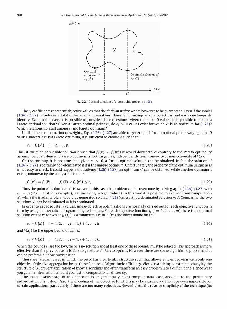
Fig. 2.2. Optimal solutions of ε-constraint problems (1.26).
The εi coefficients represent objective values that the decision maker wants however to be guaranteed. Even if the model(1.26)–(1.27) introduces a total order among alternatives, there is no mixing among objectives and each one keeps itsidentity. Even in this case, it is possible to consider these questions: given the εi > 0 values, it is possible to obtain aPareto optimal solution? Given a Pareto optimal point x∗, do εi > 0 values exist for which x∗ is an optimum for (1.25)?Which relationship exist among εi and Pareto optimum?
Unlike linear combination of weights, Eqs. (1.26)–(1.27) are able to generate all Pareto optimal points varying εi > 0values. Indeed if x∗ is a Pareto optimum, it is sufficient to choose ε such that:
εi = fix∗
i = 2, . . . , p. (1.28)
Thus if exists an admissible solution x such that f1 (x) < f1 (x∗) it would dominate x∗ contrary to the Pareto optimalityassumption of x∗. Hence no Pareto optimum is lost varying εi, independently from convexity or non-convexity of f (X).
On the contrary, it is not true that, given εi > 0, a Pareto optimal solution can be obtained. In fact the solution of(1.26)–(1.27) is certainly non-dominated if it is the unique optimum. Unfortunately the property of the optimumuniquenessis not easy to check. It could happens that solving (1.26)–(1.27), an optimum x∗ can be obtained, while another optimum xexists, unknown by the analyst, such that:
f1x∗
= f1 (x) , f2 (x) < f2x∗
≤ ε2. (1.29)
Thus the point x∗ is dominated. However in this case the problem can be overcome by solving again (1.26)–(1.27) withε2 = f2 (x∗) − 1 (if for example f2 assumes only integer values). In this way it is possible to exclude from computationx∗, while if x is admissible, it would be generated solving (1.26) (unless it is a dominated solution yet). Comparing the twosolutions x∗ can be eliminated as it is dominated.
In order to get adequate εi values, single-objective optimizations are normally carried out for each objective function inturn by using mathematical programming techniques. For each objective function fi (i = 1, 2, . . . ,m) there is an optimalsolution vector x∗
i for which fix∗
i
is a minimum. Let be fi
x∗
i
the lower bound on i.e.:
εi ≥ fix∗
i
i = 1, 2, . . . , j − 1, j + 1, . . . , k (1.30)
and fi(x∗
j ) be the upper bound on εi, i.e.:
εi ≤ fix∗
j
i = 1, 2, . . . , j − 1, j + 1, . . . , k. (1.31)
When the bounds εi are too low, there is no solution and at least one of these boundsmust be relaxed. This approach is moreeffective than the previous as it is able to generate all Pareto optima. However there are some algorithmic problems thatcan be preferable linear combination.
There are relevant cases in which the set X has a particular structure such that allows efficient solving with only oneobjective. Objective aggregation keeps these features of algorithmic efficiency. Vice versa adding constraints, changing thestructure of X , prevent application of know algorithms and often transform an easy problem into a difficult one. Hence whatyou gain in information amount you lost in computational efficiency.
The main disadvantage of this approach is its (potentially high) computational cost, also due to the preliminaryindividuation of εi values. Also, the encoding of the objective functions may be extremely difficult or even impossible forcertain applications, particularly if there are too many objectives. Nevertheless, the relative simplicity of the technique (its

G. Chiandussi et al. / Computers and Mathematics with Applications 63 (2012) 912–942 921
Fig. 3.1. A typical loosely-coupled, or ‘‘black-box’’, relationship between DAKOTA and the simulation code.
main advantage) has made it popular among some researchers (particularly in the engineering field). More information onthis method can be found in [6,17].
2.4. MOGA
The JEGA library [18] contains two global optimization methods. The first is a Multi-Objective Genetic Algorithm(MOGA) which performs Pareto optimization. The second is a Single-Objective Genetic Algorithm (SOGA) which performsoptimization on a single-objective function. Both methods support general constraints and a mixture of real and discretevariables.
Evolutionary algorithms are based on Darwin’s theory of survival of the fittest. This kind of algorithm starts with arandomly selected population of design points in the parameter space, where the values of the design parameters forma ‘genetic string’ analogous to DNA in a biological system that uniquely represents each design point in the population. Thenthemethod follows a sequence of generations,where the best design points in the population (i.e., those having lowobjectivefunction values, in case of minimization) are considered to be the most ‘fit’ and are allowed to survive and reproduce. Thealgorithm simulates the evolutionary process by employing themathematical analogs of processes such as natural selection,breeding, and mutation. Ultimately, the method identifies a design point (or a family of design points) that minimizes theobjective function of the optimization problem.
Evolutionary algorithms seem particularly suitable to solve multi-objective optimization problems because they dealsimultaneously with a set of possible solutions (the so-called population). This allows to find several members of the Paretooptimal set in a single ‘run’ of the algorithm, instead of having to perform a series of separate runs as in the case of thetraditional mathematical programming techniques. The main disadvantage is the computational cost that is in general veryhigh, this is due to the operational process of the method itself.
3. Benchmark description and analysis
The evaluation of the methods previously described has been carried out by solving five selected benchmarksrepresentative of the different possible Pareto fronts (concave, convex, linear, discontinuous) and particular attentionhas been paid to their effectiveness in terms of number of evaluations required. In order to solve the benchmarkoptimization problems the program DAKOTA (Design Analysis Kit for Optimization and Terascale Applications, SandiaNational Laboratories) has been used (Fig. 3.1). DAKOTA provides for a flexible, extensible interface between any simulationcode and a variety of iterativemethods and strategies and implements a small variety of techniques to solvemulti-objectiveoptimization problems as:
1. linear combination of weights method (see Section 2.2)2. MOGA method (see Section 2.4)
These two methods show several disadvantages. So, in order to include more effective techniques in the performancecomparison, two of them have been implemented within the DAKOTA program:
3. global criterion method (see Section 2.1)4. ε-constraint method (see Section 2.3).
In the following section, the proposed benchmarks will be described and the results obtained by applying the proposedmulti-objective techniques are shown.
922 G. Chiandussi et al. / Computers and Mathematics with Applications 63 (2012) 912–942
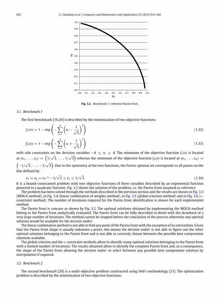
Fig. 3.2. Benchmark 1: reference Pareto front.
3.1. Benchmark 1
The first benchmark [19,20] is described by the minimization of two objective functions:
f1(x) = 1 − exp
−
3i=1
xi −
1√3
2
(1.32)
f2(x) = 1 − exp
−
3i=1
xi +
1√3
2
(1.33)
with side constraints on the decision variables −4 ≤ xi ≤ 4. The minimum of the objective function f1(x) is locatedat (x1, . . . , xn) =
1/
√3, . . . , 1/
√3whereas the minimum of the objective function f2(x) is located at (x1, . . . , xn) =
−1/√3, . . . ,−1/
√3. Due to the symmetry of the two functions, the Pareto optimal set corresponds to all points on the
line defined by:
x1 = x2 = x3 ∩ −1/√3 ≤ x1 ≤ 1/
√3. (1.34)
It is a bound-constrained problem with two objective functions of three variables described by an exponential functionpowered to a quadratic function. Fig. 3.2 shows the solution of the problem, i.e. the Pareto front assumed as reference.
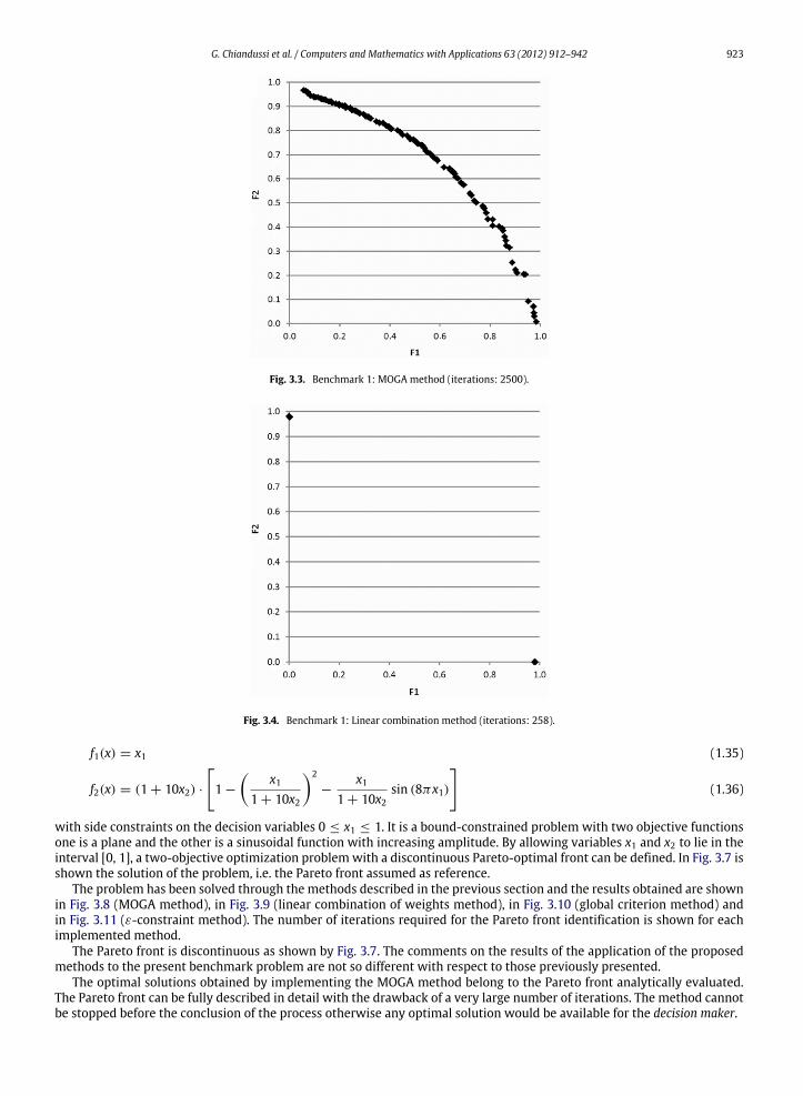
The problem has been solved through themethods described in the previous section and the results are shown in Fig. 3.3(MOGA method), in Fig. 3.4 (linear combination of weights method), in Fig. 3.5 (global criterion method) and in Fig. 3.6 (ε-constraint method). The number of iterations required for the Pareto front identification is shown for each implementedmethod.
The Pareto front is concave as shown by Fig. 3.2. The optimal solutions obtained by implementing the MOGA methodbelong to the Pareto front analytically evaluated. The Pareto front can be fully described in detail with the drawback of avery large number of iterations. The method cannot be stopped before the conclusion of the process otherwise any optimalsolution would be available for the decision maker.
The linear combinationmethod is not able to find any point of the Pareto frontwith the exception of its extremities. Giventhat the Pareto front shape is usually unknown a priori, this means the decision maker is not able to figure out the otheroptimal solutions belonging to the Pareto front and is not able to correctly choose between the possible best compromisesolutions available.
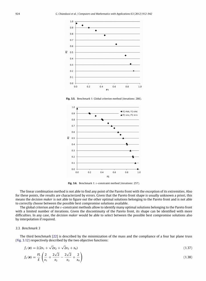
The global criterion and the ε-constraint methods allow to identify many optimal solutions belonging to the Pareto frontwith a limited number of iterations. The results obtained allow to identify the complete Pareto front and, as a consequence,the shape of the Pareto front allowing the decision maker to select between any possible best compromise solution byinterpolation if required.
3.2. Benchmark 2
The second benchmark [20] is a multi-objective problem constructed using Deb’s methodology [21]. The optimizationproblem is described by the minimization of two objective functions:
G. Chiandussi et al. / Computers and Mathematics with Applications 63 (2012) 912–942 923
Fig. 3.3. Benchmark 1: MOGA method (iterations: 2500).
Fig. 3.4. Benchmark 1: Linear combination method (iterations: 258).
f1(x) = x1 (1.35)
f2(x) = (1 + 10x2) ·
1 −
x1
1 + 10x2
2
−x1
1 + 10x2sin (8πx1)
(1.36)
with side constraints on the decision variables 0 ≤ x1 ≤ 1. It is a bound-constrained problem with two objective functionsone is a plane and the other is a sinusoidal function with increasing amplitude. By allowing variables x1 and x2 to lie in theinterval [0, 1], a two-objective optimization problemwith a discontinuous Pareto-optimal front can be defined. In Fig. 3.7 isshown the solution of the problem, i.e. the Pareto front assumed as reference.
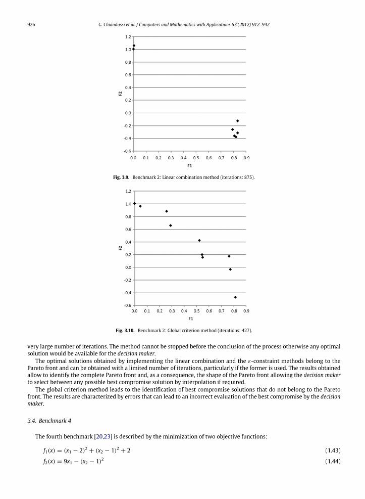
The problem has been solved through the methods described in the previous section and the results obtained are shownin Fig. 3.8 (MOGA method), in Fig. 3.9 (linear combination of weights method), in Fig. 3.10 (global criterion method) andin Fig. 3.11 (ε-constraint method). The number of iterations required for the Pareto front identification is shown for eachimplemented method.
The Pareto front is discontinuous as shown by Fig. 3.7. The comments on the results of the application of the proposedmethods to the present benchmark problem are not so different with respect to those previously presented.
The optimal solutions obtained by implementing the MOGA method belong to the Pareto front analytically evaluated.The Pareto front can be fully described in detail with the drawback of a very large number of iterations. The method cannotbe stopped before the conclusion of the process otherwise any optimal solution would be available for the decision maker.
924 G. Chiandussi et al. / Computers and Mathematics with Applications 63 (2012) 912–942
Fig. 3.5. Benchmark 1: Global criterion method (iterations: 286).
Fig. 3.6. Benchmark 1: ε-constraint method (iterations: 257).
The linear combination method is not able to find any point of the Pareto front with the exception of its extremities. Alsofor these points, the results are characterized by errors. Given that the Pareto front shape is usually unknown a priori, thismeans the decision maker is not able to figure out the other optimal solutions belonging to the Pareto front and is not ableto correctly choose between the possible best compromise solutions available.
The global criterion and the ε-constraint methods allow to identify many optimal solutions belonging to the Pareto frontwith a limited number of iterations. Given the discontinuity of the Pareto front, its shape can be identified with moredifficulties. In any case, the decision maker would be able to select between the possible best compromise solutions alsoby interpolation if required.
3.3. Benchmark 3
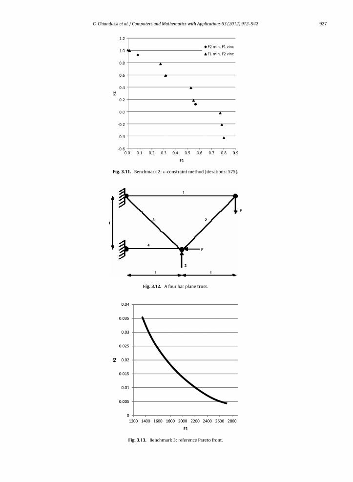
The third benchmark [22] is described by the minimization of the mass and the compliance of a four bar plane truss(Fig. 3.12) respectively described by the two objective functions:
f1 (x) = L(2x1 +√2x2 +
√2x3 + x4) (1.37)
f2 (x) =FLE
2x1
+2√2
x2−
2√2
x3+
2x4
(1.38)

G. Chiandussi et al. / Computers and Mathematics with Applications 63 (2012) 912–942 925
Fig. 3.7. Benchmark 2: reference Pareto front.
Fig. 3.8. Benchmark 2: MOGA method (iterations: 3000).
with side constraints on the decision variables:
(F/σ) ≤ x1 ≤ 3 (F/σ) (1.39)√2 (F/σ) ≤ x2 ≤ 3 (F/σ) (1.40)
√2 (F/σ) ≤ x2 ≤ 3 (F/σ) (1.41)
(F/σ) ≤ x4 ≤ 3 (F/σ) (1.42)
where the design variables are the cross-sectional areas of the bars and F = 10 kN, E = 2× 10⁵ kN/cm2, L = 200 cm, σ =
10 kN/cm2.The problem has been solved through themethods described in the previous sections and the results obtained are shown
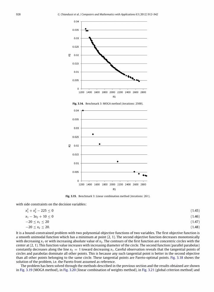
in Fig. 3.14 (MOGA method), in Fig. 3.15 (linear combination of weights method), in Fig. 3.16 (global criterion method) andin Fig. 3.17 (ε-constraint method). The number of iterations required for the Pareto front identification is shown for eachimplemented method.
The Pareto front is convex as shown by Fig. 3.13. The optimal solutions obtained by implementing the MOGA methodbelong to the Pareto front analytically evaluated. The Pareto front can be fully described in detail with the drawback of a
926 G. Chiandussi et al. / Computers and Mathematics with Applications 63 (2012) 912–942
Fig. 3.9. Benchmark 2: Linear combination method (iterations: 875).
Fig. 3.10. Benchmark 2: Global criterion method (iterations: 427).
very large number of iterations. The method cannot be stopped before the conclusion of the process otherwise any optimalsolution would be available for the decision maker.
The optimal solutions obtained by implementing the linear combination and the ε-constraint methods belong to thePareto front and can be obtained with a limited number of iterations, particularly if the former is used. The results obtainedallow to identify the complete Pareto front and, as a consequence, the shape of the Pareto front allowing the decision makerto select between any possible best compromise solution by interpolation if required.
The global criterion method leads to the identification of best compromise solutions that do not belong to the Paretofront. The results are characterized by errors that can lead to an incorrect evaluation of the best compromise by the decisionmaker.
3.4. Benchmark 4
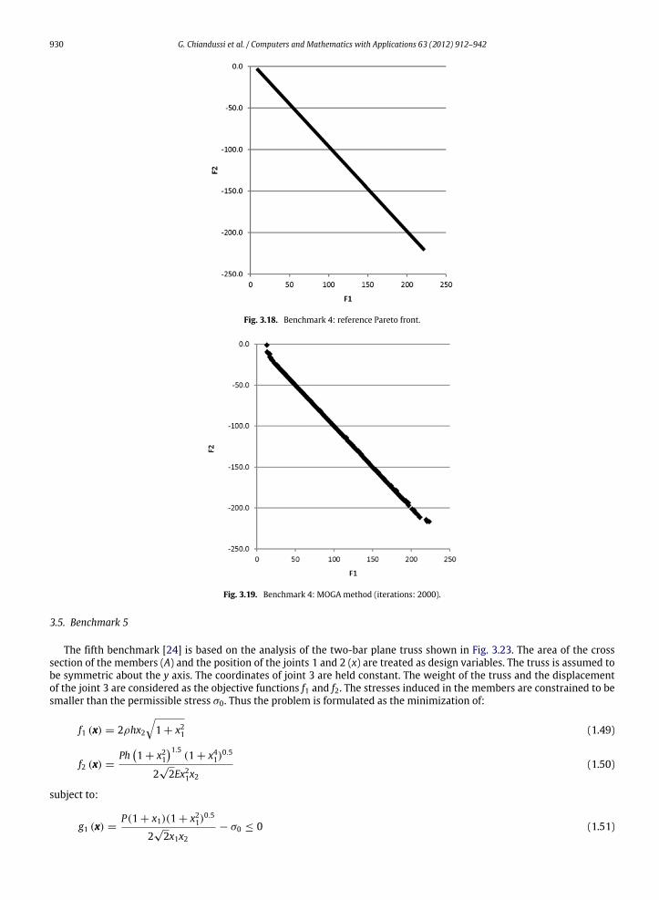
The fourth benchmark [20,23] is described by the minimization of two objective functions:
f1(x) = (x1 − 2)2 + (x2 − 1)2 + 2 (1.43)
f2(x) = 9x1 − (x2 − 1)2 (1.44)
G. Chiandussi et al. / Computers and Mathematics with Applications 63 (2012) 912–942 927
Fig. 3.11. Benchmark 2: ε-constraint method (iterations: 575).
2
4
I
I I
F
F
23
1
Fig. 3.12. A four bar plane truss.
Fig. 3.13. Benchmark 3: reference Pareto front.
928 G. Chiandussi et al. / Computers and Mathematics with Applications 63 (2012) 912–942
Fig. 3.14. Benchmark 3: MOGA method (iterations: 2500).
Fig. 3.15. Benchmark 3: Linear combination method (iterations: 261).
with side constraints on the decision variables:
x21 + x22 − 225 ≤ 0 (1.45)
x1 − 3x2 + 10 ≤ 0 (1.46)−20 ≤ x1 ≤ 20 (1.47)−20 ≤ x2 ≤ 20. (1.48)
It is a bound-constrained problem with two polynomial objective functions of two variables. The first objective function isa smooth unimodal function which has a minimum at point (2, 1). The second objective function decreases monotonicallywith decreasing x1 or with increasing absolute value of x2. The contours of the first function are concentric circles with thecenter at (2, 1). This function value increases with increasing diameter of the circle. The second function (parallel parabolas)constantly decreases along the line x2 = 1 toward decreasing x1. Careful observation reveals that the tangential points ofcircles and parabolas dominate all other points. This is because any such tangential point is better in the second objectivethan all other points belonging to the same circle. These tangential points are Pareto-optimal points. Fig. 3.18 shows thesolution of the problem, i.e. the Pareto front assumed as reference.
The problem has been solved through the methods described in the previous section and the results obtained are shownin Fig. 3.19 (MOGA method), in Fig. 3.20 (linear combination of weights method), in Fig. 3.21 (global criterion method) and

G. Chiandussi et al. / Computers and Mathematics with Applications 63 (2012) 912–942 929
Fig. 3.16. Benchmark 3: Global criterion method (iterations: 450).
Fig. 3.17. Benchmark 3: ε-constraint method (iterations: 704).
in Fig. 3.22 (ε-constraint method). The number of iterations required for the Pareto front identification is shown for eachimplemented method.
The Pareto front is linear, to say, concave and convex at the same time, as shown by Fig. 3.18. The optimal solutionsobtained by implementing the MOGA method belong to the Pareto front analytically evaluated. The Pareto front can befully described in detail with the drawback of a very large number of iterations. The method cannot be stopped before theconclusion of the process otherwise any optimal solution would be available for the decision maker.
The linear combinationmethod is not able to find any point of the Pareto frontwith the exception of its extremities. Giventhat the Pareto front shape is usually unknown a priori, this means the decision maker is not able to figure out the otheroptimal solutions belonging to the Pareto front and is not able to correctly choose between the possible best compromisesolutions available.
The global criterion and the ε-constraint methods allow to identify many optimal solutions belonging to the Pareto frontwith a limited number of iterations. The results obtained allow to identify the complete Pareto front and, as a consequence,the shape of the Pareto front allowing the decision maker to select between any possible best compromise solution byinterpolation if required.
930 G. Chiandussi et al. / Computers and Mathematics with Applications 63 (2012) 912–942
Fig. 3.18. Benchmark 4: reference Pareto front.
Fig. 3.19. Benchmark 4: MOGA method (iterations: 2000).
3.5. Benchmark 5
The fifth benchmark [24] is based on the analysis of the two-bar plane truss shown in Fig. 3.23. The area of the crosssection of the members (A) and the position of the joints 1 and 2 (x) are treated as design variables. The truss is assumed tobe symmetric about the y axis. The coordinates of joint 3 are held constant. The weight of the truss and the displacementof the joint 3 are considered as the objective functions f1 and f2. The stresses induced in the members are constrained to besmaller than the permissible stress σ0. Thus the problem is formulated as the minimization of:
f1 (x) = 2ρhx21 + x21 (1.49)
f2 (x) =Ph1 + x21
1.5(1 + x41)
0.5
2√2Ex21x2
(1.50)
subject to:
g1 (x) =P(1 + x1)(1 + x21)
0.5
2√2x1x2
− σ0 ≤ 0 (1.51)
G. Chiandussi et al. / Computers and Mathematics with Applications 63 (2012) 912–942 931
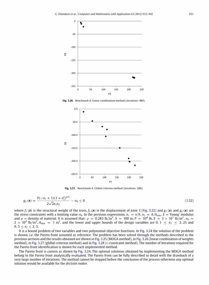
Fig. 3.20. Benchmark 4: Linear combination method (iterations: 480).
Fig. 3.21. Benchmark 4: Global criterion method (iterations: 288).
g2 (x) =P(−x1 + 1)(1 + x21)
0.5
2√2x1x2
− σ0 ≤ 0 (1.52)
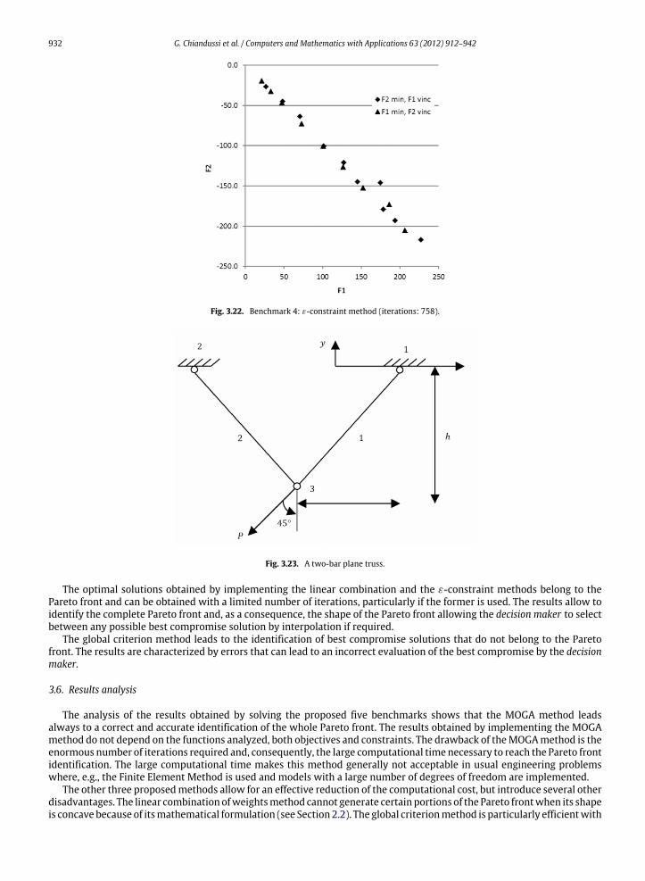
where f1 (x) is the structural weight of the truss, f2 (x) is the displacement of joint 3 (Fig. 3.22) and g1 (x) and g2 (x) arethe stress constraints with a limiting value σ0. In the previous expressions, x1 = x/h, x2 = A/Amin, E = Young’ modulusand ρ = density of material. It is assumed that: ρ = 0.283 lb/in3, h = 100 in, P = 104 lb, E = 3 × 10⁷ lb/in2, σ0 =
2 × 10⁴ lb/in2, Amin = 1 in2, and the lower and upper bounds of the design variables are 0, 1 ≤ x1 ≤ 2, 25 and0, 5 ≤ x2 ≤ 2, 5.
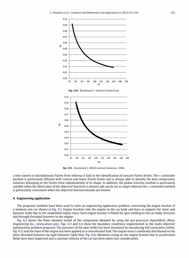
It is a bound problem of two variables and two polynomial objective functions. In Fig. 3.24 the solution of the problemis shown, i.e. the Pareto front assumed as reference. The problem has been solved through the methods described in theprevious sections and the results obtained are shown in Fig. 3.25 (MOGAmethod), in Fig. 3.26 (linear combination ofweightsmethod), in Fig. 3.27 (global criterion method) and in Fig. 3.28 (ε-constraint method). The number of iterations required forthe Pareto front identification is shown for each implemented method.
The Pareto front is convex as shown by Fig. 3.24. The optimal solutions obtained by implementing the MOGA methodbelong to the Pareto front analytically evaluated. The Pareto front can be fully described in detail with the drawback of avery large number of iterations. The method cannot be stopped before the conclusion of the process otherwise any optimalsolution would be available for the decision maker.
932 G. Chiandussi et al. / Computers and Mathematics with Applications 63 (2012) 912–942
Fig. 3.22. Benchmark 4: ε-constraint method (iterations: 758).
Fig. 3.23. A two-bar plane truss.
The optimal solutions obtained by implementing the linear combination and the ε-constraint methods belong to thePareto front and can be obtained with a limited number of iterations, particularly if the former is used. The results allow toidentify the complete Pareto front and, as a consequence, the shape of the Pareto front allowing the decision maker to selectbetween any possible best compromise solution by interpolation if required.
The global criterion method leads to the identification of best compromise solutions that do not belong to the Paretofront. The results are characterized by errors that can lead to an incorrect evaluation of the best compromise by the decisionmaker.
3.6. Results analysis
The analysis of the results obtained by solving the proposed five benchmarks shows that the MOGA method leadsalways to a correct and accurate identification of the whole Pareto front. The results obtained by implementing the MOGAmethod do not depend on the functions analyzed, both objectives and constraints. The drawback of theMOGAmethod is theenormous number of iterations required and, consequently, the large computational time necessary to reach the Pareto frontidentification. The large computational time makes this method generally not acceptable in usual engineering problemswhere, e.g., the Finite Element Method is used and models with a large number of degrees of freedom are implemented.
The other three proposedmethods allow for an effective reduction of the computational cost, but introduce several otherdisadvantages. The linear combination ofweightsmethod cannot generate certain portions of the Pareto frontwhen its shapeis concave because of itsmathematical formulation (see Section 2.2). The global criterionmethod is particularly efficientwith
G. Chiandussi et al. / Computers and Mathematics with Applications 63 (2012) 912–942 933
Fig. 3.24. Benchmark 5: reference Pareto front.
Fig. 3.25. Benchmark 5: MOGA method (iterations: 3000).
a non-convex or discontinuous Pareto front whereas it fails in the identification of concave Pareto fronts. The ε-constraintmethod is particularly efficient with convex and linear Pareto fronts and is always able to identify the best compromisesolutions belonging to the Pareto front independently of its shape. In addition, the global criterion method is particularlysuitable when the ideal value of the objective functions is known and can be set as target whereas the ε-constraint methodis particularly convenient when the objective function bounds are known.
4. Engineering application
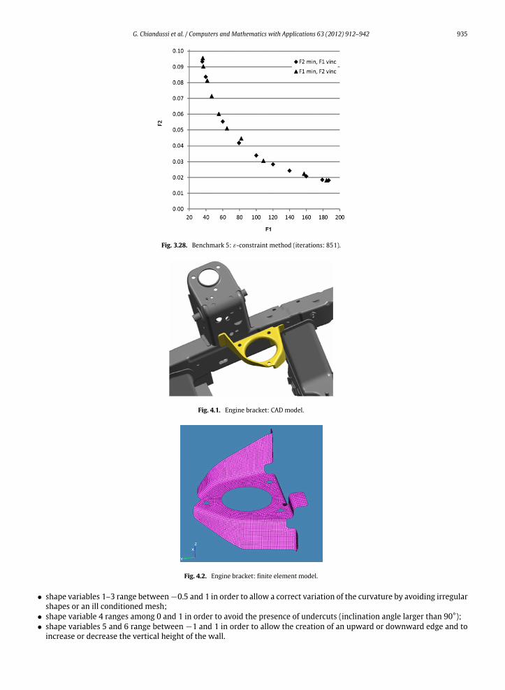
The proposed methods have been used to solve an engineering application problem concerning the engine bracket ofa medium size car shown in Fig. 4.1. Engine brackets link the engine to the car body and have to support the static anddynamic loads due to the suspended engine mass. Each engine bracket is linked by spot welding to the car body structureand through threaded fasteners to the engine.
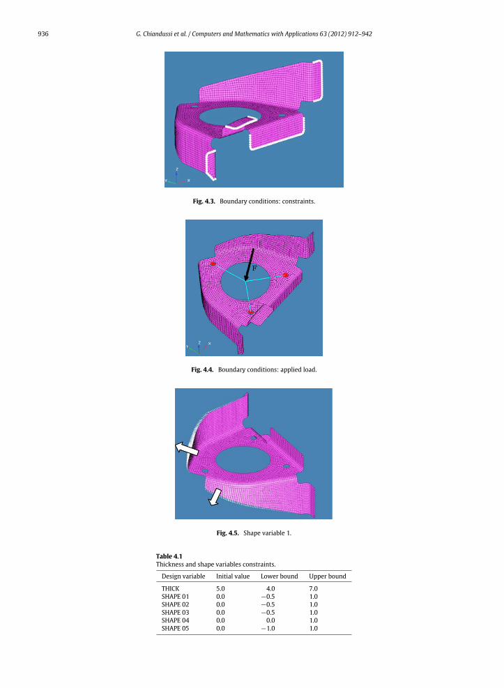
Fig. 4.2 shows the finite element model of the component obtained by using the pre-processor HyperMesh (AltairEngineering Inc., www.altair.com). Figs. 4.3 and 4.4 show the boundary conditions implemented in the multi-objectiveoptimization problem proposed. The presence of the spot welds has been simulated by introducing full constraints (white,Fig. 4.3) and themass of the engine has been applied as a concentrated load. The enginemass is uniformly distributed on thethree threaded fasteners by rigid elements (light blue, Fig. 4.4). Moments acting on the engine bracket due to accelerationfields have been neglected and a constant velocity of the car has been taken into consideration.

934 G. Chiandussi et al. / Computers and Mathematics with Applications 63 (2012) 912–942
Fig. 3.26. Benchmark 5: Linear combination method (iterations: 273).
Fig. 3.27. Benchmark 5: Global criterion method (iterations: 405).
The properties of the material the bracket is made of (steel) are:
• material density: ρ = 7850 kg/m3.• Young’s modulus: E = 205 000 MPa.• Poisson ratio: ν = 0.3.• yield stress: σy = 460 MPa.• ultimate stress: σu = 520 MPa.
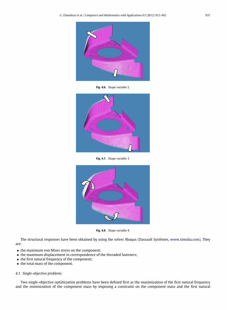
The engine bracket is manufactured by forming and bending a sheet metal plate of uniform thickness. As a consequence,the sheet metal thickness and its initial shape can be modified by taking into account the available space. Shape variableshave been defined by a morphing process by preserving the partial symmetry of the component due to the use of the samemold for production cost reduction. Figs. 4.5–4.7 show three shape variables that allow tomodify the curvature of the verticalwalls of the component. Fig. 4.8 shows the shape variable that allows to modify the inclination of the vertical walls. Fig. 4.9shows the shape variables that allows to create a circular edge at the internal radius of the central hole of the component.Finally Fig. 4.10 shows the shape variable that allows to modify the height of the vertical wall.
Design variable values have been bound by taking into account theworking conditions of the component, the productiontechnologies and the objectives of the optimization problem, i.e. mass minimization and frequency maximization. Thethickness value ranges between 4 and 7mmas required by the productive process. Shapes variables instead vary in a suitablerange according to component geometry (Table 4.1):
G. Chiandussi et al. / Computers and Mathematics with Applications 63 (2012) 912–942 935
Fig. 3.28. Benchmark 5: ε-constraint method (iterations: 851).
Fig. 4.1. Engine bracket: CAD model.
Fig. 4.2. Engine bracket: finite element model.
• shape variables 1–3 range between−0.5 and 1 in order to allow a correct variation of the curvature by avoiding irregularshapes or an ill conditioned mesh;
• shape variable 4 ranges among 0 and 1 in order to avoid the presence of undercuts (inclination angle larger than 90°);• shape variables 5 and 6 range between −1 and 1 in order to allow the creation of an upward or downward edge and to
increase or decrease the vertical height of the wall.
936 G. Chiandussi et al. / Computers and Mathematics with Applications 63 (2012) 912–942
Fig. 4.3. Boundary conditions: constraints.
Fig. 4.4. Boundary conditions: applied load.
Fig. 4.5. Shape variable 1.
Table 4.1Thickness and shape variables constraints.
Design variable Initial value Lower bound Upper bound
THICK 5.0 4.0 7.0SHAPE 01 0.0 −0.5 1.0SHAPE 02 0.0 −0.5 1.0SHAPE 03 0.0 −0.5 1.0SHAPE 04 0.0 0.0 1.0SHAPE 05 0.0 −1.0 1.0
G. Chiandussi et al. / Computers and Mathematics with Applications 63 (2012) 912–942 937
Fig. 4.6. Shape variable 2.
Fig. 4.7. Shape variable 3.
Fig. 4.8. Shape variable 4.
The structural responses have been obtained by using the solver Abaqus (Dassault Systèmes, www.simulia.com). Theyare:
• the maximum von Mises stress on the component;• the maximum displacement in correspondence of the threaded fasteners;• the first natural frequency of the component;• the total mass of the component.
4.1. Single-objective problems
Two single-objective optimization problems have been defined first as the maximization of the first natural frequencyand the minimization of the component mass by imposing a constraint on the component mass and the first natural

938 G. Chiandussi et al. / Computers and Mathematics with Applications 63 (2012) 912–942
Fig. 4.9. Shape variable 5.
Fig. 4.10. Shape variable 6.
Table 4.2Design variable, objective function and constraint values: first natural frequency maximization problem optimal solution.
Design variable Optimal value Objective function Optimal value
THICK 6.89 FREQ 01 1051 HzSHAPE 01 −0.27SHAPE 02 −0.49 Design constraint ValueSHAPE 03 −0.33 MAX STRESS 204 MPaSHAPE 04 0.36 MAX DISPL 0.08 mmSHAPE 05 0.67 MASS 1.89 kgSHAPE 06 −0.88
frequency, respectively. Then a multi-objective optimization problem looking for the first natural frequency maximizationand the component mass minimization has been defined and solved.
4.1.1. First natural frequency maximizationThe first single-objective optimization problem has been defined as the maximization of the first natural frequency of
the component with constraints on the global mass, the maximum Von Mises stress and the maximum displacement of theconnection points with the engine:
maximize: I natural frequency (FREQ 01)subject to: Von Mises stress (MAX STRESS) < 368 MPa
displacement (MAX DISPL) < 0.4 mmmass (MASS) < 1.9 kg
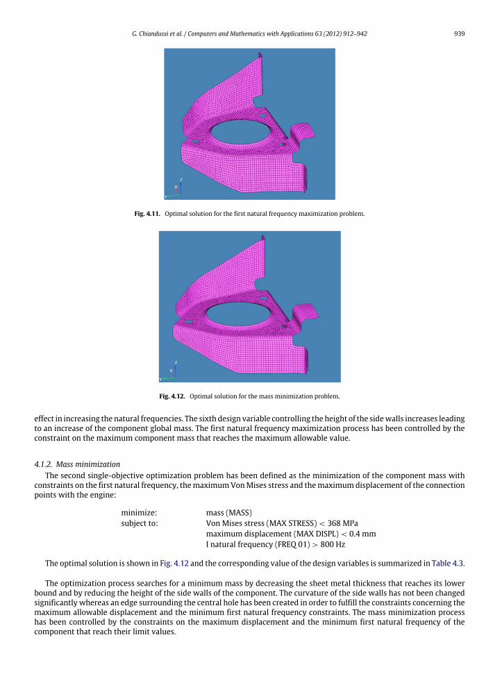
The optimal solution is shown in Fig. 4.11 and the value of the design variables, of the objective function and of theconstraints is summarized in Table 4.2.
The sheet metal thickness approaches the upper bound of 7 mm, shape variables 1–3 provide for a small modification ofthe side wall geometry while the fourth shape variable provides for a small inclination. The fifth shape variable controllingthe height of a possible edge surrounding the central hole of the component shows a meaningful change due to its positive
G. Chiandussi et al. / Computers and Mathematics with Applications 63 (2012) 912–942 939
Fig. 4.11. Optimal solution for the first natural frequency maximization problem.
Fig. 4.12. Optimal solution for the mass minimization problem.
effect in increasing the natural frequencies. The sixth design variable controlling the height of the sidewalls increases leadingto an increase of the component global mass. The first natural frequency maximization process has been controlled by theconstraint on the maximum component mass that reaches the maximum allowable value.
4.1.2. Mass minimizationThe second single-objective optimization problem has been defined as the minimization of the component mass with
constraints on the first natural frequency, themaximumVonMises stress and themaximumdisplacement of the connectionpoints with the engine:
minimize: mass (MASS)subject to: Von Mises stress (MAX STRESS) < 368 MPa
maximum displacement (MAX DISPL) < 0.4 mmI natural frequency (FREQ 01) > 800 Hz
The optimal solution is shown in Fig. 4.12 and the corresponding value of the design variables is summarized in Table 4.3.
The optimization process searches for a minimum mass by decreasing the sheet metal thickness that reaches its lowerbound and by reducing the height of the side walls of the component. The curvature of the side walls has not been changedsignificantly whereas an edge surrounding the central hole has been created in order to fulfill the constraints concerning themaximum allowable displacement and the minimum first natural frequency constraints. The mass minimization processhas been controlled by the constraints on the maximum displacement and the minimum first natural frequency of thecomponent that reach their limit values.

940 G. Chiandussi et al. / Computers and Mathematics with Applications 63 (2012) 912–942
Table 4.3Design variable, objective function and constraint values: mass minimization problem optimal solution.
Design variable Optimal value Objective function Optimal value
THICK 5.11 MASS 1.34 kgSHAPE 01 −0.37SHAPE 02 −0.47 Design constraint ValueSHAPE 03 0.03 MAX STRESS 333 MPaSHAPE 04 0.11 MAX DISPL 0.18 mmSHAPE 05 0.50 FREQ 01 823 HzSHAPE 06 0.74
Fig. 4.13. MOGA method (iterations: 1000).
Fig. 4.14. Linear combination method (iterations: 612).
4.2. Multi-objective problem
The results of the single-objective optimization problems previously presented show that the maximization of the firstnatural frequency and the minimization of the mass of the engine bracket are competing objectives and that a multi-objective optimization problem is worth to be implemented in order to identify the complete set of optimal compromisesolutions represented by the Pareto front.
The multi-objective optimization problem has been set up as:
minimize: mass (MASS)maximize: I natural frequency (FREQ 01)subject to: Von Mises stress (MAX STRESS) < 368 MPa
displacement (MAX DISPL) < 0.4 mm
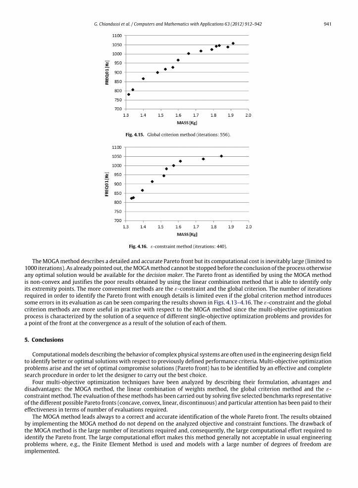
It is a bound problem with two polynomial objective functions, two constraints on structural responses and 7 designvariables. The problem has been solved through the methods described in previous sections and the results are shown inFig. 4.13 (MOGA method), in Fig. 4.14 (linear combination of weights), in Fig. 4.15 (global criterion method) and in Fig. 4.16(ε-constraint method).
G. Chiandussi et al. / Computers and Mathematics with Applications 63 (2012) 912–942 941
Fig. 4.15. Global criterion method (iterations: 556).
Fig. 4.16. ε-constraint method (iterations: 440).
TheMOGAmethod describes a detailed and accurate Pareto front but its computational cost is inevitably large (limited to1000 iterations). As already pointed out, theMOGAmethod cannot be stoppedbefore the conclusion of the process otherwiseany optimal solution would be available for the decision maker. The Pareto front as identified by using the MOGA methodis non-convex and justifies the poor results obtained by using the linear combination method that is able to identify onlyits extremity points. The more convenient methods are the ε-constraint and the global criterion. The number of iterationsrequired in order to identify the Pareto front with enough details is limited even if the global criterion method introducessome errors in its evaluation as can be seen comparing the results shown in Figs. 4.13–4.16. The ε-constraint and the globalcriterion methods are more useful in practice with respect to the MOGA method since the multi-objective optimizationprocess is characterized by the solution of a sequence of different single-objective optimization problems and provides fora point of the front at the convergence as a result of the solution of each of them.
5. Conclusions
Computationalmodels describing the behavior of complex physical systems are often used in the engineering design fieldto identify better or optimal solutions with respect to previously defined performance criteria. Multi-objective optimizationproblems arise and the set of optimal compromise solutions (Pareto front) has to be identified by an effective and completesearch procedure in order to let the designer to carry out the best choice.
Four multi-objective optimization techniques have been analyzed by describing their formulation, advantages anddisadvantages: the MOGA method, the linear combination of weights method, the global criterion method and the ε-constraintmethod. The evaluation of thesemethods has been carried out by solving five selected benchmarks representativeof the different possible Pareto fronts (concave, convex, linear, discontinuous) and particular attention has been paid to theireffectiveness in terms of number of evaluations required.
The MOGA method leads always to a correct and accurate identification of the whole Pareto front. The results obtainedby implementing the MOGA method do not depend on the analyzed objective and constraint functions. The drawback ofthe MOGA method is the large number of iterations required and, consequently, the large computational effort required toidentify the Pareto front. The large computational effort makes this method generally not acceptable in usual engineeringproblems where, e.g., the Finite Element Method is used and models with a large number of degrees of freedom areimplemented.
942 G. Chiandussi et al. / Computers and Mathematics with Applications 63 (2012) 912–942
The linear combination of weights and the global criterionmethods allow for an effective reduction of the computationalcost, but introduce several other advantages and disadvantages. The linear combination of weights method cannot generatecertain portions of the Pareto front when its shape is concave because of its mathematical formulation. The global criterionmethod is particularly suitable when the ideal value of the objective functions is known and can be set as target, it isparticularly efficient in the identification of non-convex or discontinuous Pareto fronts, but it fails in the identification ofconcave Pareto fronts.
The ε-constraint method allows for an effective reduction of the computational cost. It is particularly convenient whenthe objective function bounds are known and it is particularly efficientwith convex and linear Pareto fronts. The ε-constraintmethod is always able to identify the best compromise solutions belonging to the Pareto front independently of its shape.
The Pareto front of common multi-objective engineering optimization problems is usually unknown a priori. If theevaluation of the objective and constraint functions is computationally expensive, it is necessary to implement optimizationmethods able to identify the shape of the Pareto front with a reduced number of evaluations. The ε-constraint methodshowed the best results and, as a consequence, has to be preferred in this kind of applications.
References
[1] T. Bäck, D.B. Fogel, Z. Michalewicz (Eds.), Evolutionary Algorithms in Theory and Practice, Institute of Physics Publications, Bristol, 2000.[2] M. Ehrgott, Multicriteria Optimization, Springer, Berlin, 2000.[3] A. Osyczka, Multicriteria optimization for engineering design, in: A. Osyczka (Ed.), Design Optimization, Academic Press, 1985, pp. 193–227.[4] C.A. Coello Coello, Theoretical and numerical constraint-handling techniques used with evolutionary algorithms: a survey of the state of the art,
Comput. Methods Appl. Mech. Engrg. 191 (2002) 1245–1287.[5] J.L. Cohon, D.H. Marks, A review and evaluation of multiobjective programming techniques, Water Resour. Res. 11 (1975) 208–220.[6] A. Osyczka, Multicriterion Optimization in Engineering with FORTRAN Programs, John Wiley & Sons, New York, 1984.[7] L.M. Boychuk, V.O. Ovchinnikov, Principal methods of solution of multicriterial optimization problems, Sov. Automat. Control 6 (1973) 1–4.[8] M.E. Salukvadze, On the existence of solution in problems of optimization, J. Optim. Theory Appl. 13 (1974) 203–217.[9] K. Koski, Multicriterion optimization in structural design, in: A. Atrek (Ed.), New Directions in Optimum Structural Design, 1984.
[10] L. Duckstein, Multiobjective optimization in structural design: the model, in: A. Atrek (Ed.), New Directions in Optimum Structural Design, 1984.[11] A.P. Wierzbicki, On the use of penalty functions in multiobjective optimization, in: Proceedings of the International Symposium on Operations
Research, 1978.[12] M. Zeleny, Compromise programming, in: M. Zeleny (Ed.), Multiple Criteria Decision Making, 1973.[13] J.L. Cochrane, M. Zeleny (Eds.), Multiple Criteria Decision Making, McGraw-Hill Book Company, New York, 1982.[14] L.A. Zadeh, Optimality and nonscalar-valued performance criteria, IEEE Trans. Automat. Control 8 (1963) 59–60.[15] S. Gass, T.L. Saaty, The computational algorithm for the parametric objective function, Naval Res. Logist. Quart. 2 (1955) 39–45.[16] L. Lasdon, D.Wismer, Y. Haimes, On a bicriterion formulation of the problems of integrated system identification and system optimization, IEEE Trans.
Syst. Man Cybern. 1 (1971) 296–297.[17] Z. Lounis, M.Z. Cohn, Multiobjective optimization of prestressed concrete structures, J. Struct. Eng. ASCE 119 (1993) 794–809.[18] K. Lewis, J.E. Eddy, Effective generation of Pareto sets using genetic programming, in: Proceedings of ASME Design Engineering Technical Conference,
2001.[19] P.J. Fleming, C.M. Fonseca, Multiobjective genetic algorithms made easy: selection, sharing, and mating restriction, in: Proceedings of the First
International Conference on Genetic Algorithms in Engineering Systems: Innovations and Applications, 1995.[20] C.A. Coello Coello, G.B. Lamont, D.A. Van Veldhuizen, Evolutionary Algorithms for Solving Multi-Objective Problems, Springer, New York, 2007.[21] K. Deb, Multi-objective genetic algorithms: problem difficulties and construction of test problems, Evol. Comput. 7 (1999) 205–230.[22] C.A. Coello Coello, A short tutorial on evolutionary multiobjective optimization, in: E. Zitzler, K. Deb, L. Thiele, C.A. Coello Coello, D. Corne (Eds.), First
International Conference on Evolutionary Multi-Criterion Optimization, Springer-Verlag, 2001.[23] N. Srinivas, K. Deb, Multiobjective optimization using nondominated sorting in genetic algortihms, Evol. Comput. 2 (1994) 221–248.[24] S.S. Rao, Game theory approach for multiobjective structural optimization, Comput. Struct. 25 (1987) 119–127.