computing effective tax rates in presence of non … · computing effective tax rates in presence...

istatworkingpapers

N.92015

Computing Effective Tax Rates in presence of Non-linearityin Corporate Taxation

Antonella Caiumi, Lorenzo Di Biagio, Marco Rinaldi

N.92015

Computing Effective Tax Rates in presence of Non-linearityin Corporate Taxation

Antonella Caiumi, Lorenzo Di Biagio, Marco Rinaldi

istatworkingpapers

Comitato scientifico

Giorgio Alleva Emanuele Baldacci Francesco Billari Tommaso Di Fonzo Andrea Mancini Roberto Monducci Fabrizio Onida Linda Laura Sabbadini Antonio Schizzerotto

Comitato di redazione

Alessandro Brunetti Patrizia Cacioli Marco Fortini Romina Fraboni Stefania Rossetti Daniela Rossi Maria Pia Sorvillo

Segreteria tecnica

Daniela De Luca Laura Peci Marinella Pepe Gilda Sonetti

Istat Working Papers Computing Effective Tax Rates in presence of Non-Linearity in Corporate Taxation N. 9/2015 ISBN 978-88-458-1836-3 © 2015 Istituto nazionale di statistica Via Cesare Balbo, 16 – Roma Salvo diversa indicazione la riproduzione è libera, a condizione che venga citata la fonte. Immagini, loghi (compreso il logo dell’Istat), marchi registrati e altri contenuti di proprietà di terzi appartengono ai rispettivi proprietari e non possono essere riprodotti senza il loro consenso.

ISTAT WORKING PAPERS N. 9/2015

Computing Effective Tax Rates in presence of Non-linearity inCorporate Taxation 1

Antonella Caiumi 2, Lorenzo Di Biagio 3, Marco Rinaldi 4

Sommario

Questo articolo presenta il calcolo delle aliquote effettive di imposta forward-looking utilizzandol’approccio di Devereux–Griffith in presenza di limiti alla deducibilità e riporti in avanti delle quotenon dedotte di specifiche componenti della base imponibile. Per quanto ne sappiamo questo è il primocontributo su questo tema. Più precisamente vengono misurati gli effetti sull’incentivazione agli in-vestimenti di un limite alla deducibilità degli interessi basato sull’EBITDA (utili prima degli interessi,delle imposte e degli ammortamenti) della società. Si mostra come l’approccio di Devereux–Griffithpossa essere impiegato anche in questo caso specifico e si calcola il cuneo d’imposta al variare deicoefficienti di ammortamento e del tasso di interesse. Inoltre, in presenza di un regime d’impostadel tipo ACE, si analizzano le implicazioni sulle scelte di finanziamento dell’impresa associate allaintroduzione della limitazione alla deducibilità degli interessi. Più in generale, è stato predispostouno specifico programma per il calcolo delle aliquote effettive d’imposta per qualsiasi forma, anchenon lineare, della funzione del prelievo fiscale sui profitti.

Parole Chiave: Tassazione societaria; Costo del capitale; Aliquote effettive di imposta;Metodologia di Devereux–Griffith; Deducibilità degli interessi; Aiuto alla crescita economica.

Abstract

The focus of this paper is how forward-looking effective tax rates can be computed in the presenceof ceilings and carryovers in the taxable base using the Devereux–Griffith approach. As far as isknown, this is the first contribution on this issue. More specifically, the paper examines the impacton investment incentives of a new treatment of interest expense which sets a ceiling, defined in termsof the firm’s EBITDA, on net deductible interest expense allowing both non-deductible interests andunused EBITDA carryovers. The effects that interest deduction caps have on effective tax rates arenot at all negligible. Further, the analysis illustrates the implications of the limitation on interestdeductibility on the choice of funding by comparing alternative tax regime: a profit tax and an al-lowance for corporate equity (ACE) tax regime. Finally, a toolkit that allows to tackle any form ofnon-linear tax liabilities function is developed.

Keywords: Corporate taxation; Cost of capital; Effective tax rates; Devereux–Griffith methodol-ogy; Interest deductibility rules; Allowance for corporate equity.

1 Paper presented at the “Giornate della ricerca in Istat 2014”, 10th-11th of November 2014, Roma, Italy. The views expressed in thispaper are those of the authors and do not necessarily represent the institutions with which they are affiliated. Any errors or mistakesremain the authors’ sole responsibility.

2 DIQR — Servizio Studi Econometrici e Previsioni economiche — email: [email protected] DIQR — Servizio Studi Econometrici e Previsioni economiche — email: [email protected] DICS — Servizio Statistiche Strutturali sulle Imprese e le Istituzioni — email: [email protected]

ISTITUTO NAZIONALE DI STATISTICA 5

mailto:[email protected]



COMPUTING EFFECTIVE TAX RATES IN PRESENCE OF NON-LINEARITY IN CORPORATE TAXATION

Contents

1. Introduction . . . . . . . . . . . . . . . . . . . . . . . . . . . . . . . . . . . . . . 7

2. The Devereux–Griffith model in a domestic setting . . . . . . . . . . . . . . . . . 8

3. Conceptual framework to calculate forward-looking effective tax rates in thepresence of ceilings in the taxable base . . . . . . . . . . . . . . . . . . . . . . . 9

4. A numerical analysis . . . . . . . . . . . . . . . . . . . . . . . . . . . . . . . . . . 13

5. Concluding remarks . . . . . . . . . . . . . . . . . . . . . . . . . . . . . . . . . . 16

A An example — the Italian case . . . . . . . . . . . . . . . . . . . . . . . . . . . . 17

B Effective tax rates in a domestic setting using the Devereux-Griffith approach . . 19

6 ISTITUTO NAZIONALE DI STATISTICA


1. Introduction

A country’s tax regime is a key policy instrument that may negatively or positively influence in-vestments. Policy analysts should regularly assess the tax burden on profits to determine whetherthe tax system is supportive of business investments. Forward-looking approaches are designed tocapture incentives to undertake new investment projects and involve computing the effective tax bur-den for hypothetical future investment projects using statutory features of the tax regimes. Theseapproaches are suitable for international comparisons and are tailored to disentangle the effects ofspecific provisions of the tax legislation, by providing an indication of general patterns of tax incen-tives to investments.

The most commonly used forward-looking concepts for analyzing the impact of taxation on in-vestment behaviour are the Effective Marginal Tax Rate (EMTR) and the Effective Average Tax Rates(EATR). Originally proposed by King and Fullerton (1984), the EMTR captures the effect of the leg-islative tax parameters on an incremental business activity and shows how much to invest on themargin given a diminishing expected return on investment. The EATR, further developed by Dev-ereux and Griffith (1998, 2003), summarizes the proportion of the expected total profits taken in taxesand shows the effect of the tax regime on a total investment project (national or international). Thislatter indicator is a more suitable measure than the EMTR for a highly profitable multinational toadopt when deciding where to invest, and a more general tax burden indicator in the analysis of theinternational location of capital.

Methods for computing EMTR and EATR have been extensively used in recent years to comparethe effective tax rates levied on capital income from different domestic investments over time andacross countries (OECD 1991, EEC 2001, Devereux et al. 2009, Bilicka et al. 2011, OECD 2013,Suzuki 2014, Spengel et al. 2014). Main statutory provisions usually taken into account in forward-looking tax burden indicators include – beyond statutory tax rates – capital depreciation allowances,cost allowance from taxable base, tax credits, the interest expense deducibility and so on. However,the synthetic measures computed so far do not allow to fully capture the complexity and heterogeneityof tax incentive schemes. For example, the tax burden consequences of carryovers schemes (i.e.,losses carry forward or carry back, tax allowances carry forward) or the presence of ceilings on thedeductibility of interest expense are typically ignored in this kind of analysis.

This paper contributes to fill the gap by extending the computation of effective marginal andaverage tax rates to incorporate earning-stripping style rules which introduce non-linearity in thetax liability function. New rules on interest deduction limitations have been recently enacted orproposed in several jurisdictions. Some of them apply only to potentially abusive situations, suchas related party debt or the financing of shareholdings benefiting from a participation exemption.In this cases limitations are designed to avoid artificial allocation of financial resources within agroup of companies aimed at reallocating income and expense within the group in order to benefitfrom tax arbitrage among jurisdictions with different tax rates and regulations, or between companieswith and without tax credits. Other restrictions are in principle broader in scope being part of basebroadening reforms and extended to all taxpayers. For example Germany, Italy and Spain, haverecently overhauled their interest deduction rules based on a debt-to-equity test in favor of moreeffective interest barrier rules that allow interest deduction up to a fixed interest to income ratio.5The majority of countries which currently seek to address base erosion and profit shifting are alsoconsidering similar modifications (OECD, 2015). Recent theoretical and empirical findings also arguethe relevance of interest deductibility rules in a tax competition environment (Altshuler and Grubert2006, Haufler and Runkel 2012).

In particular, in this paper we develop the case of an interest deductibility rule that sets a ceiling onnet deductible interest at a fixed percentage of EBITDA in each period allowing both non-deductibleinterests and unused EBITDA carry forwards. Because of non-linearity in the tax liability functionit is no longer possible to compute the cost of capital separately for each asset and source of financeand then just take a weighted mean. We closely follow the Devereux–Griffith conceptual framework,however we rely on an additional assumption. Specifically, we assume that when the new treatment

5 Detailed description of a number of existing thin capitalization rules is given by Webber (2010).



of interest expense is introduced a value-maximizing firm adjusts its indebtedness to exploit the per-mitted amount of interest deductions to the fullest possible extent, so as to avoid interest add-backs.Once the new investment is being undertaken, the binding constraint may turn out to be violated de-pending on the combination of sources of finance chosen. We show under which circumstances thisassumption holds. Then, the expression for the post-tax economic rent and the cost of capital underthe Devereux–Griffith methodology is derived.

Our model framework receives support from recent empirical studies on the effectiveness of thincapitalization rules on multinational firm capital structure (Buettner et al. 2012, Blouin et al. 2014).In particular, Blouin et al. (2014) show that MNEs respond quickly to the introduction of restric-tions to the deductibility of interest expense. In contrast, the empirical literature on the impact oftax incentives on investment decisions find no evidence of negative investment effects in relation tointerest barrier rules (Weichenrieder and Windischbauer 2008, Buslei and Simmler 2012). While thiscould be possibly due to a number of factors including the ability of multinational firms to exploitloopholes in the legislation, our analysis illustrates that the effects of interest barrier rules on tax in-vestment incentives are significant, although there is great variability in the effects in relation to fiscaldepreciation rules. We argue that incorporating interest barrier rules in the evaluation of tax invest-ment incentive may give rise to significant changes in the ranking across countries (see Appendix Afor some insights).

Differently from other studies (Zangari, 2009), our analysis does not rely on a fix parameterfor the share of deductible interest expense. To show this, we examine the implications of interestdeductibility restrictions on financing and investment decisions considering two alternative corporatetax regimes: a profit tax and an allowance for corporate equity. For these selected cases we computeeffective marginal and average tax rates solving for the firm optimal debt ratio. Besides, to tackle anyform of non-linear tax liability function we develop a toolkit that implicitly computes the post-taxeconomic rent as well as the associated ETRs. This allows us to evaluate the impact of interest barrierrules in combination with other aspects of the tax code on the competitiveness of the tax system as awhole.

The paper is organized as follows. In Section 2 we briefly introduce the Devereux–Griffith modelin a domestic context. In Section 3 we illustrate the assumptions and the procedures underlying thecalculation of the effective tax rates in the presence of a non-linear tax liabilities function. In Section4 we examine the implications of introducing a partial interests deductibility rule within two differenttax regimes, a profit tax and an incremental ACE. Section 5 concludes.

2. The Devereux–Griffith model in a domestic setting

The standard approach to compute measures of effective marginal and average tax rates is basedon the following assumptions. Consider a profit-maximizing firm. In period t the firm increasescapital stock Kt and investment It by one unit choosing among different sources of finance (or acombination of them): retained earnings, new equity or debt. In period t + 1 the addition to Kt

generates a change in output ∆Q = p+ δ and a change in net revenue of ∆Qt+1 = (p+ δ)(1 + π),where π is the inflation rate and δ is the economic depreciation rate. In period t the additionalinvestment is dismissed such that ∆It+1 = −(1 − δ)(1 + π). Contextually the debt (principal andinterests) is reimbursed and the new equity repurchased at the original price. In the case of retainedearnings, the investment is financed by a corresponding reduction in dividends, Dt. The additionalpost-tax net return is distributed as dividends to shareholders at time t + 1. Typically, it is assumedthat the firm is not tax-exhausted so as to exploit any form of tax advantage.

The net present value of post-tax economic rent, Rt realized at time t is defined as the change inthe firm equity value, Vt:

Vt =γDt −Nt + Vt+1

1 + ρ,

where ρ is the shareholders’ nominal discount rate, γ is the measure of the tax discrimination betweennew equity and distribution, Dt is the dividend paid in period t and Nt is the new equity issued in



period t. After some algebraic manipulations we get the present value of the firm at time t

(1 + ρ)Vt =+∞∑s=0

γDt+s −Nt+s

(1 + ρ)s, (1)

and so

Rt := (1 + ρ)∆Vt =

+∞∑s=0

γ∆Dt+s −∆Nt+s

(1 + ρ)s. (2)

Dividends Dt are the residuals of the model and are defined as

Dt = Qt(Kt−1) +Nt − It +Bt − (1 + i)Bt−1 − Tt, (3)

where Qt(Kt−1) is output in period t which depends on the beginning of period capital stock Kt−1,It is the investment at time t, Bt is one-period debt issued at time t, i is the nominal interest rate(risk is ignored), and Tt is the tax liability at time t. In the case of a profit tax, Tt takes the followingexpression

Tt = τ(Qt(Kt−1)− φ

(It +KT

t−1

)− iBt−1

), (4)

where τ is the statutory tax rate on profits and φ is the rate at which capital expenditure can be offsetagainst tax and KT

t−1 is the tax-written-down value of capital stock.Solving the Devereux–Griffith framework allows one to compute the effective tax rates (ETRs)

which encompasses both EMTR for a marginal investment and the EATR for different levels of prof-itability. The EMTR is obtained setting the post-tax economic rent, Rt, to zero and solving it for p,thus deriving the minimum pre-tax real rate of return p̃, i.e., the cost of capital. The EATR can bemeasured for different values of the pre-tax real rate of return p higher than the minimum pre-tax rateof return required in order to undertake the investment, p̃. Both effective marginal and average taxrates depend on the statutory tax rate and the definition of the tax base, however the EMTR dependson the tax base to a greater degree. 6

3. Conceptual framework to calculate forward-looking effective tax rates in the pres-ence of ceilings in the taxable base

Suppose a limitation on interest deductibility comes into force. The new rule sets a ceilingon net deductible interest in each period allowing both non-deductible interests and ceiling left-overs carry forwards. Let Gt denote the ceiling on interests deduction at time t defined as apercentage α of the Gross Operating Profit (GOP).7 Notice that Qt provides a close approxima-tion for the GOP, then Gt = min {iBt−1, αQt} in the simplified case of no carryovers. Tak-ing into account for both unused GOP and interest add-backs carryovers, Gt can be expressed asGt = min

{iBt−1 + [Mt]

− , αQt + [Mt]+}, where Mt is the GOP excess at time t − 1 (if positive)

or the excess of interest expense (if negative). As usual, [·]+ indicates the positive part, and [·]− thenegative part, i.e., [a]+ := max{0, a}, [a]− := −min{0, a}.

It is assumed that when the firm becomes aware that a new treatment of interest expense willcome into force then it adjusts its debt ratio in the long-run path to take full advantage of the de-ductibility of interest expense, thus avoiding to sustain non-deductible interests. First, it is provedthat this assumption holds in the more general case of an ACE tax regime. Then, it is shown how theDevereux–Griffith approach can still be applied to compute the ETRs.

The firm’s tax liability function is modified as follows

6 Refer to Appendix B for a detail illustration of the formal Devereux–Griffith model and the computation of the ETRs in a domesticsetting.

7 The definition of GOP is closer to the EBITDA and corresponds to the difference between item A (Production Value) and item B(Production Costs) in the income statement excluding depreciation and amortization of property, plant and equipment, and intangibleassets, interests and lease payments.



Tt = τ(Qt − φ(It +KTt−1)− iEEt−1 −Gt), (5)

where iE is the ACE notional rate of return, Et−1 the ACE base at time t − 1 (i.e., the share of owncapital that grants the ACE allowance) and τiEEt−1 is the ACE deduction. In order to incorporate anypossible depreciation scheme, we denote by Lt, instead of φ(It +KT

t−1), the depreciation allowancesin period t.

At time t = 0 the company becomes aware that in period t = 1 either the GOP rule or the ACEregime, or both will come into force. Prior to undertake the hypothetical investment, the firm followsa long-run path that consists in maintaining its capital stock constant in each year, Kt = K0 (inflationis not considered) by replacing the economic depreciation, It = δK0. Then the production Qt is keptconstant over time Qt = Q0. At time t = 0 the firm adjusts the combination of funding to maximizethe post-tax income, i.e., B0 6= B−1. Then for every t ≥ 0, Bt is constantly equal to B0. To simplifynotation, in Proposition 1, it is assumed that retained earnings are the only source of internal finance.

Proposition 1. If both an ACE regime and a GOP rule are in force and the following condition holdsρ−iτ ≤ iE ≤ i+ ρ−i

τ , then a profit-maximizing firm will incur interest expense up to the ceiling set bythe tax rule.

Proof. In Equation (1) substitute Equation (3) at t = 0. Since ε :=∑+∞

s=01

(1+ρ)s = ρ+1ρ we obtain

(1 + ρ)V0 = εγQ0 − εγδK0 + γB0 −γi

ρB0 − γiB−1 − γB−1 −

+∞∑s=0

γTs(1 + ρ)s

.

By Equation (5), we need to specifyEs andGs, i.e., the ACE base and the GOP rule. The incrementalACE base can be expressed as follows:

Es =

[I0 −B0 +B−1 +

s∑n=1

(In − (Bn −Bn−1))

]+

and by the assumption that the indebtedness is kept constant over time we get

Es = (s+ 1)δK0 −B0 +B−1,

for every s ≥ 0. As for Gs, notice that the equation of motion of Ms is

Ms+1 = αQs − iBs−1 +Ms,

with M0 = M1 = 0, hence Ms = (s− 1)(αQ0 − iB0) for each s ≥ 2.Therefore G0 = 0 and for each s ≥ 1

Gs = min{iB0 + [Ms]−, αQ0 + [Ms]

+} =

= min{iB0 + [(s− 1)(αQ0 − iB0)]−, αQ0 + [(s− 1)(αQ0 − iB0)]+}.

If αQ0 − iB0 ≥ 0 then Gs = min{iB0, αQ0 + c} = iB0, while if αQ0 − iB0 ≤ 0 then Gs =min{iB0 + c′, αQ0} = αQ0, where c, c′ are positive constants. Thus Gs = min{iB0, αQ0}, as inthe simpler case of carryforwards not allowed.

It follows thatT0 = τ (Q0 − L0)

andTs = τQ0 − τiE(sδK0 −B0 +B−1)− τ min{αQ0, iB0} − τLs, for s ≥ 1.

Since the net present value of capital depreciation allowances∑+∞

s=0γτLs

(1+ρ)s is finite (see Appendix Bfor further insights) then

(1 + ρ)V0 = γB0 −γi

ρB0 −

γτhiEρ

B0 +γτhρ

min{αQ0, iB0}+ C,

where C is a constant that does not depend on B0. The result follows.



If personal taxation is not considered, or more generally if the personal tax rate on interest incomeis equal to the tax rate on capital gains, then ρ = i (see Appendix B) and the following holds:

Corollary 2. If both an ACE regime and a GOP rule are in force, and the ACE notional rate of returniE is less than, or equal to, the nominal interest rate i, then a value-maximizing firm adjusts its debtratio in order to incur interest expense up to the ceiling set by the tax rule.

Corollary 2 allows to state that in the presence of the limitation on interest deduction the firm inits long-run path incurs interest expense just up to the allowed ceiling.8

In what follows we show how to compute ETRs following the Devereux–Griffith procedure. Attime t the hypothetical investment is undertaken. From Corollary 2, provided that i ≥ iE , the changein the tax liability takes the following expression:

∆Tt = τ (∆Qt − iE∆Et−1 −min{i∆Bt−1, α∆Qt} −∆Lt) .

We substitute γ∆Dt+s−∆Nt+s for each s ≥ 0. At time t: γ∆Dt−∆Nt = −γ+γ∆Bt−∆Nt(1−γ) + γτ∆Lt. At time t+ 1:

1

1 + ρ(γ∆Dt+1 −∆Nt+1) =

γ

1 + ρ((1 + π)(p+ δ)(1− τ) + (1 + π)(1− δ)− (1 + i)∆Bt) +

+γ

1 + ρ(τiE∆Et + τ min {i∆Bt, α(1 + π)(p+ δ)}) +

− 1

1 + ρ∆Nt+1(1− γ) +

γ

1 + ρτ∆Lt+1.

At time t+ s, with s ≥ 2: 1(1+ρ)s (γ∆Dt+s −∆Nt+s) = γ

(1+ρ)s τ∆Lt+s.

The post-tax economic rent Rt of the incremental investment can then be derived from Equation(2). Rt can be split into two parts: Rt = RRE

t + Ft, where RREt is common to all sources of finance

while Ft changes with the source of finance9

RREt = −γ +

γ

1 + ρ((1 + π)(p+ δ)(1− τ) + (1 + π)(1− δ)) + γτ

+∞∑s=0

∆Lt+s(1 + ρ)s

, (6)

Ft = γ∆Bt

(1− 1 + i

1 + ρ

)+

γ

1 + ρτ (iE∆Et + min {i∆Bt, α(1 + π)(p+ δ)}) + (7)

− (1− γ)∆Nt

(1− 1

1 + ρ

).

If the ACE allowance is not considered (iE = 0) then

Ft = γ∆Bt

(1− 1 + i

1 + ρ

)+

γ

1 + ρτ (min {i∆Bt, α(1 + π)(p+ δ)})− (1− γ)∆Nt

(1− 1

1 + ρ

).

In Table 1 are listed all the changes in the sources of funding.In the presence of the GOP rule, raising debt at time t to finance the hypothetical investment

may cause interest expense to exceed the allowed ceiling at time t+ 1 depending on the profitabilityrate which, in turn, affects the GOP rule. At time t + 2 the investment is reversed and the bindingconstraint of the interest deductibility rule is restored. Notice that because of the GOP rule, Rt is nolonger linear in p. It is rather a broken line, and the point at which Rt breaks depends on the debtratio and the economic and fiscal depreciation allowances of the asset purchased.

8 Notice that Corollary 2 clearly holds also in the absence of an ACE regime (i.e., iE = 0).9 Since an ACE allowance is considered it is not longer true that Ft includes only the additional cost of raising external finance; Ft is

now different from zero in the case of retained earnings. See (Bresciani and Giannini, 2003, par. 2.1).



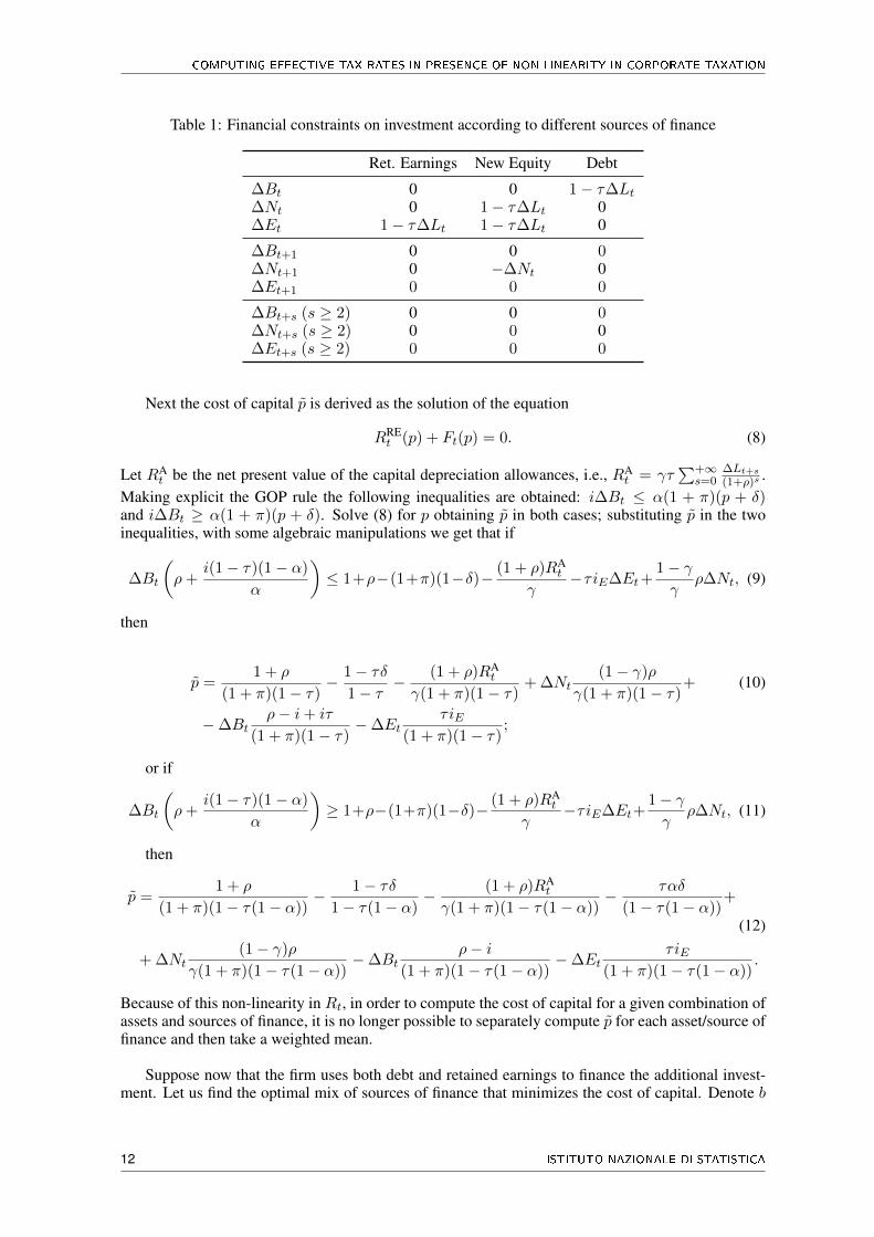
Table 1: Financial constraints on investment according to different sources of finance

Ret. Earnings New Equity Debt

∆Bt 0 0 1− τ∆Lt∆Nt 0 1− τ∆Lt 0∆Et 1− τ∆Lt 1− τ∆Lt 0

∆Bt+1 0 0 0∆Nt+1 0 −∆Nt 0∆Et+1 0 0 0

∆Bt+s (s ≥ 2) 0 0 0∆Nt+s (s ≥ 2) 0 0 0∆Et+s (s ≥ 2) 0 0 0

Next the cost of capital p̃ is derived as the solution of the equation

RREt (p) + Ft(p) = 0. (8)

Let RAt be the net present value of the capital depreciation allowances, i.e., RA

t = γτ∑+∞

s=0∆Lt+s(1+ρ)s .

Making explicit the GOP rule the following inequalities are obtained: i∆Bt ≤ α(1 + π)(p + δ)and i∆Bt ≥ α(1 + π)(p + δ). Solve (8) for p obtaining p̃ in both cases; substituting p̃ in the twoinequalities, with some algebraic manipulations we get that if

∆Bt

(ρ+

i(1− τ)(1− α)

α

)≤ 1+ρ−(1+π)(1−δ)− (1 + ρ)RA

t

γ−τiE∆Et+

1− γγ

ρ∆Nt, (9)

then

p̃ =1 + ρ

(1 + π)(1− τ)− 1− τδ

1− τ− (1 + ρ)RA

t

γ(1 + π)(1− τ)+ ∆Nt

(1− γ)ρ

γ(1 + π)(1− τ)+ (10)

−∆Btρ− i+ iτ

(1 + π)(1− τ)−∆Et

τiE(1 + π)(1− τ)

;

or if

∆Bt

(ρ+

i(1− τ)(1− α)

α

)≥ 1+ρ−(1+π)(1−δ)− (1 + ρ)RA

t

γ−τiE∆Et+

1− γγ

ρ∆Nt, (11)

then

p̃ =1 + ρ

(1 + π)(1− τ(1− α))− 1− τδ

1− τ(1− α)− (1 + ρ)RA

t

γ(1 + π)(1− τ(1− α))− ταδ

(1− τ(1− α))+

(12)

+ ∆Nt(1− γ)ρ

γ(1 + π)(1− τ(1− α))−∆Bt

ρ− i(1 + π)(1− τ(1− α))

−∆EtτiE

(1 + π)(1− τ(1− α)).

Because of this non-linearity in Rt, in order to compute the cost of capital for a given combination ofassets and sources of finance, it is no longer possible to separately compute p̃ for each asset/source offinance and then take a weighted mean.

Suppose now that the firm uses both debt and retained earnings to finance the additional invest-ment. Let us find the optimal mix of sources of finance that minimizes the cost of capital. Denote b



the debt ratio, then from Table 1, ∆Bt = (1 − τ∆Lt)b, ∆Nt = 0 and ∆Et = (1 − τ∆Lt)(1 − b).Substituting into Equation (10) and Equation (12) we obtain the cost of capital as a function of b. Ifcondition (9) holds then

p̃ = c1 + (1− τ∆Lt)i− ρ− τ(i− iE)

(1 + π)(1− τ)b.

Similarly, if condition (11) holds then

p̃ = c2 + (1− τ∆Lt)i− ρ+ τiE

(1 + π)(1− τ(1− α))b,

where c1, c2 are constants that do not depend on b. Therefore if ρ−iτ ≤ iE ≤ i + ρ−i

τ , then in theformer equation we have a negative slope for b, while in the latter a positive one. This is consistentwith Proposition 1. The minimum cost of capital p̃min is achieved when the equality holds in Equation(9) or (11), i.e., when

b(1−τ∆Lt)

(ρ+

i(1− τ)(1− α)

α− τiE

)= 1+ρ−(1+π)(1−δ)− (1 + ρ)RA

t

γ−τiE(1−τ∆Lt).

(13)Given the optimal debt ratio bopt from Equation (13), since i(1− τ∆Lt)bopt = α(1 + π)(p̃min + δ),then

p̃min =i(1− τ∆Lt)bopt

α(1 + π)− δ. (14)

4. A numerical analysis

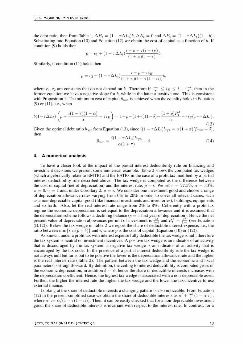
To have a closer look at the impact of the partial interest deductibility rule on financing andinvestment decisions we present some numerical example. Table 2 shows the computed tax wedges(which algebraically relate to EMTR) and the EATRs in the case of a profit tax modified by a partialinterest deductibility rule described above. The tax wedge is computed as the difference betweenthe cost of capital (net of depreciation) and the interest rate, p̃ − i. We set τ = 27.5%, α = 30%,π = 0, γ = 1 and, under Corollary 2, ρ = i. We consider one investment good and choose a rangeof depreciation allowance rates varying from 0% to 20% in order to cover all relevant cases, suchas a non-depreciable capital good (like financial investments and inventories), buildings, equipmentsand so forth. Also, let the real interest rate range from 2% to 8%. Coherently with a profit taxregime the economic depreciation is set equal to the depreciation allowance and it is assumed thatthe depreciation scheme follows a declining balance (s = 1 first year of depreciation). Hence the netpresent value of depreciation allowances per unit of investment is τδ

i+δ and RAt = τδ1+i (see Equation

(B.12)). Below the tax wedge in Table 2 we report the share of deductible interest expense, i.e., theratio between min{i, α(p̃+ δ)} and i, where p̃ is the cost of capital (Equation (10) or (12)).

As known, under a profit tax with interest expense fully deductible the tax wedge is null, thereforethe tax system is neutral on investment incentives. A positive tax wedge is an indicator of an activitythat is discouraged by the tax system; a negative tax wedge is an indicator of an activity that isencouraged by the tax code. In the presence of a partial interest deductibility rule the tax wedge isnot always null but turns out to be positive the lower is the depreciation allowance rate and the higheris the real interest rate (Table 2). The pattern between the tax wedge and the economic and fiscalparameters is straightforward. By definition, the ceiling to interest deductibility is computed gross ofthe economic depreciation, in addition δ = φ, hence the share of deductible interests increases withthe depreciation coefficient. Hence, the highest tax wedge is associated with a non-depreciable asset.Further, the higher the interest rate the higher the tax wedge and the lower the tax-incentive to useexternal finance.

Looking at the share of deductible interests a changing pattern is also noticeable. From Equation(12) in the present simplified case we obtain the share of deductible interests as α′ + αδ

i (1− α′τ) ,where α′ := α/(1− τ(1− α)). Then, it can be easily checked that for a non-depreciable investmentgood, the share of deductible interests is invariant with respect to the interest rate. In contrast, for a



Table 2: Tax wedges, EATRs and the share of deductible interests when an interest stripping rulemodifies a profit tax regime (Percentage points).

fiscal wedge EATR (p=10%)

i

δ 2% 4% 6% 8% 2% 4% 6% 8%

0% 0.48 0.95 1.43 1.91 22.00 19.25 19.25 19.25(37.2) (37.2) (37.2) (37.2) (100) (75.0) (50.0) (37.5)

5% 0 0.44 0.92 1.4 22.00 16.50 15.13 15.13(100) (70.8) (59.6) (54.0) (100) (100) (75.0) (56.3)

15% 0 0 0 0.37 22.00 16.50 11.00 6.88(100) (100) (100) (87.7) (100) (100) (100) (93.8)

20% 0 0 0 0 22.00 16.50 11.00 5.50(100) (100) (100) (100) (100) (100) (100) (100)

Note: in parenthesis the share of deductible interests

depreciable investment good, the higher the interest rate the lower the share of deductible interests.Finally, the EATRs for a profitability rate p = 10% are computed. As expected, the effective taxrates increase with the share of undeductible interests which in turn depends on how binding is theconstraint and on the level of the interest rate.10

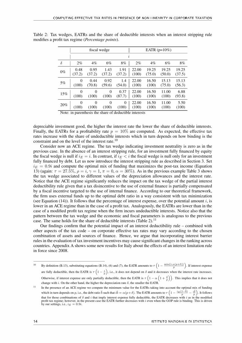
Consider now an ACE regime. The tax wedge indicating investment neutrality is zero as in theprevious case. In the absence of an interest stripping rule, for an investment fully financed by equitythe fiscal wedge is null if iE = i. In contrast, if iE < i the fiscal wedge is null only for an investmentfully financed by debt. Let us now introduce the interest stripping rule as described in Section 3. SetiE = 0.9i and compute the optimal mix of funding that maximizes the post-tax income (Equation13) (again: τ = 27.5%, ρ = i, γ = 1, π = 0, α = 30%). As in the previous example Table 3 showsthe tax wedge associated to different values of the depreciation allowances and the interest rate.Notice that the ACE regime significantly reduces the impact on the tax wedge of the partial interestdeductibility rule given that a tax disincentive to the use of external finance is partially compensatedby a fiscal incentive targeted to the use of internal finance. According to our theoretical framework,the firm uses external funds up to the optimal debt ratio in a way consistent with tax minimization(see Equation (14)). It follows that the percentage of interest expense, over the potential amount i, islower in an ACE regime than in the case of a profit tax. Analogously, the EATRs are lower than in thecase of a modified profit tax regime when the firm incurs undeductible interests. Notice also that thepattern between the tax wedge and the economic and fiscal parameters is analogous to the previouscase. The same holds for the share of deductible interests (Table 2).11

Our findings confirm that the potential impact of an interest deductibility rule – combined withother aspects of the tax code – on corporate effective tax rates may vary according to the chosencombination of assets and sources of finance. Hence, we argue that incorporating interest barrierrules in the evaluation of tax investment incentives may cause significant changes in the ranking acrosscountries. Appendix A shows some new results for Italy about the effects of an interest limitation rulein force since 2008.

10 By definition (B.13), substituting equations (B.14), (6) and (7), the EATR amounts to τ(

1− min{i,α(p+δ)}p

). If interest expense

are fully deductible, then the EATR is τ(

1− ip

), i.e., it does not depend on δ and it decreases when the interest rate increases.

Otherwise, if interest expense are only partially deductible, then the EATR is τ(

1− α(

1 + δp

)). This implies that it does not

change with i. On the other hand, the higher the depreciation rate δ, the smaller the EATR.11 In the presence of an ACE regime we compute the minimum value for the EATRs taking into account the optimal mix of funding

which in turn depends on p, i.e., the debt ratio b such that ib = α(p+δ). The EATR amounts to τ(

1− iE(1−b)p

− ibp

). It follows

that for those combinations of δ and i that imply interest expense fully deductible, the EATR decreases with i as in the modifiedprofit tax regime; however, in the present case the EATR further decreases with i even when the GOP rule is binding. This is drivenby our settings, i.e., iE = 0.9i.



Table 3: Tax wedges, EATRs and the percentage of interest expense in the presence of both an intereststripping rule and an ACE regime (Percentage points).

fiscal wedge EATR (p=10%)

i

δ 2% 4% 6% 8% 2% 4% 6% 8%

0% 0.05 0.14 0.16 0.21 22.00 16.78 11.83 6.88(30.8) (30.8) (30.8) (30.8) (100) (75.0) (50.0) (37.5)

5% 0 0.05 0.1 0.15 22.00 16.50 11.41 6.46(100) (67.9) (55.5) (49.3) (100) (100) (75.0) (56.3)

15% 0 0 0 0.04 22.00 16.50 11.00 5.64(100) (100) (100) (86.4) (100) (100) (100) (93.8)

20% 0 0 0 0 22.00 16.50 11.00 5.50(100) (100) (100) (100) (100) (100) (100) (100)

Note: in parenthesis the percentage of interest expense

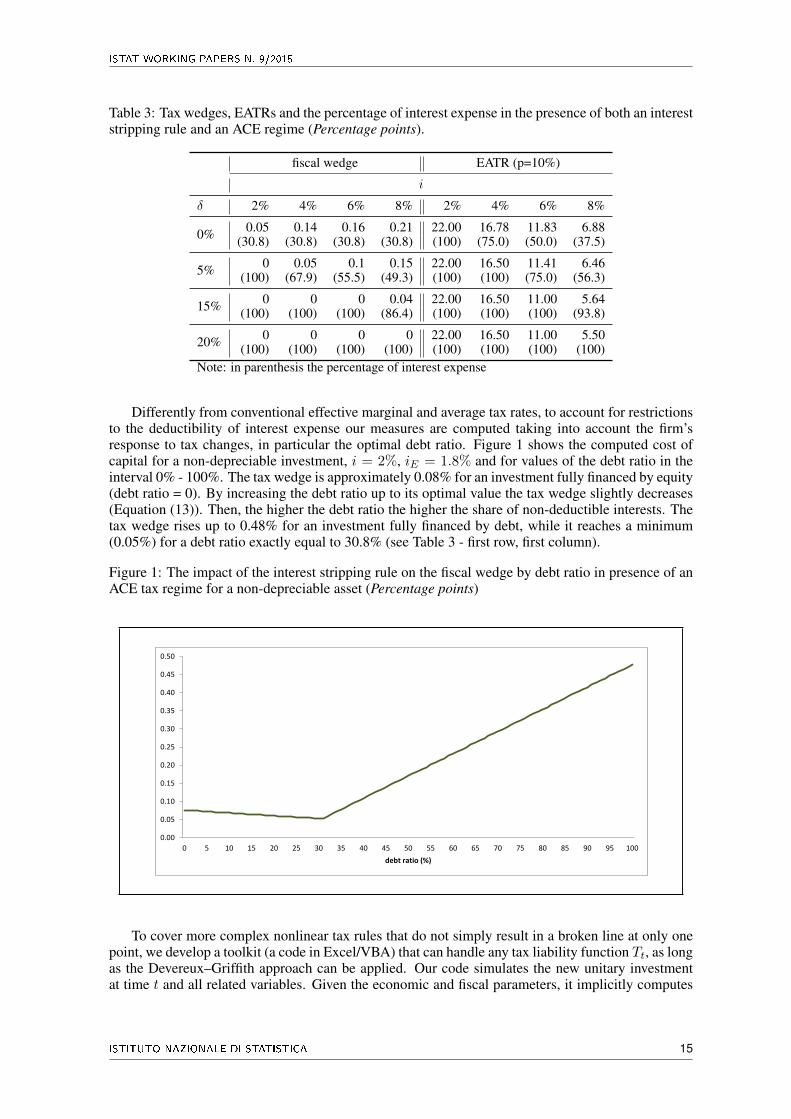
Differently from conventional effective marginal and average tax rates, to account for restrictionsto the deductibility of interest expense our measures are computed taking into account the firm’sresponse to tax changes, in particular the optimal debt ratio. Figure 1 shows the computed cost ofcapital for a non-depreciable investment, i = 2%, iE = 1.8% and for values of the debt ratio in theinterval 0% - 100%. The tax wedge is approximately 0.08% for an investment fully financed by equity(debt ratio = 0). By increasing the debt ratio up to its optimal value the tax wedge slightly decreases(Equation (13)). Then, the higher the debt ratio the higher the share of non-deductible interests. Thetax wedge rises up to 0.48% for an investment fully financed by debt, while it reaches a minimum(0.05%) for a debt ratio exactly equal to 30.8% (see Table 3 - first row, first column).

Figure 1: The impact of the interest stripping rule on the fiscal wedge by debt ratio in presence of anACE tax regime for a non-depreciable asset (Percentage points)

0.00

0.05

0.10

0.15

0.20

0.25

0.30

0.35

0.40

0.45

0.50

0 5 10 15 20 25 30 35 40 45 50 55 60 65 70 75 80 85 90 95 100

debt ratio (%)

To cover more complex nonlinear tax rules that do not simply result in a broken line at only onepoint, we develop a toolkit (a code in Excel/VBA) that can handle any tax liability function Tt, as longas the Devereux–Griffith approach can be applied. Our code simulates the new unitary investmentat time t and all related variables. Given the economic and fiscal parameters, it implicitly computes



Rt(p) for any p, any mix of assets and sources of funding. It follows that it is not necessary toalgebraically recover Rt for each function Tt: it is only required to specify the expression for Tt andmake the program run. The cost of capital is then obtained applying the secant method, a well-knownroot-finding algorithm. 12

5. Concluding remarks

This paper applies and extends the Devereux and Griffith methodology (1998, 2003) to calculateeffective marginal and average tax rates in the presence of ceilings and carryovers in the taxable base.We illustrate the potential importance of taking into account interest deductibility rules in evaluat-ing tax incentives on corporate decisions through a numerical example. We identify a clear negativeimpact on both investment and financing choices but the extent of the tax bias varies according to de-preciation allowances and the interest rate. We also show that an ACE regime reduces the disincentiveeffect of a limitation on interest deductibility, provided that the debt ratio is optimized accordingly.

As argued in other studies (Haufler and Runkel, 2012), tax provisions like interest barrier rules,that are explictly targeted at mobile capital, may be a more important determinant for multinationalenterprises’ location decisions than statutory tax rates. We deem that the omission of interest strip-ping rule in the computation of effective tax rates may lead to misleading results in internationalcomparisons on corporate tax regimes.

Also these findings suggest a much larger variation in effective tax rates at the firm level notcaptured by conventional effective tax measures. Hence, the methodology developed in this papermay prove useful in empirical analysis on the behavioural response to taxation exploiting firm-specificforward-looking effective tax rates (Egger et al., 2009). Our model could be further extended withina multiperiod framework following the approach proposed by Klemm (2012) to analyze the effectsof carryover schemes (such as losses carry forwards and tax allowances carry forward) on investmenttax incentives.

Acknowledgements

We are grateful to Sebastien Bradley, Davide Castellani, Silvia Giannini, Paolo Panteghini, par-ticipants at the 69th annual meeting of the International Institute of Public Finance (2013 IIPF), andseminar participants at the “Giornate della ricerca" in ISTAT, 10-11 November 2014, Rome, Italy forhelpful comments and suggestions to an earlier version.

12 In numerical analysis, the secant method is an iterative root-finding algorithm that uses a succession of roots of secant lines to betterapproximate a root of a function f . In our case the recurrence relation is defined as pn := pn−1−Rt(pn−1)

pn−1−pn−2

Rt(pn−1)−Rt(pn−2).



A An example — the Italian case

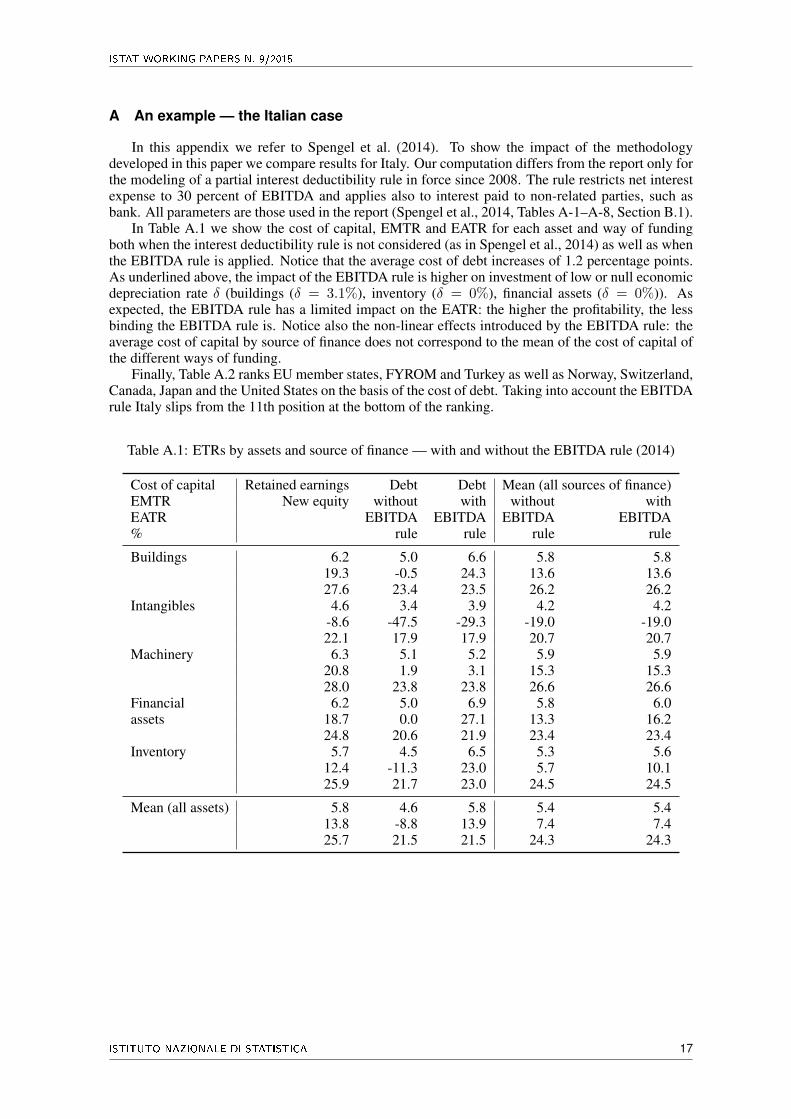
In this appendix we refer to Spengel et al. (2014). To show the impact of the methodologydeveloped in this paper we compare results for Italy. Our computation differs from the report only forthe modeling of a partial interest deductibility rule in force since 2008. The rule restricts net interestexpense to 30 percent of EBITDA and applies also to interest paid to non-related parties, such asbank. All parameters are those used in the report (Spengel et al., 2014, Tables A-1–A-8, Section B.1).

In Table A.1 we show the cost of capital, EMTR and EATR for each asset and way of fundingboth when the interest deductibility rule is not considered (as in Spengel et al., 2014) as well as whenthe EBITDA rule is applied. Notice that the average cost of debt increases of 1.2 percentage points.As underlined above, the impact of the EBITDA rule is higher on investment of low or null economicdepreciation rate δ (buildings (δ = 3.1%), inventory (δ = 0%), financial assets (δ = 0%)). Asexpected, the EBITDA rule has a limited impact on the EATR: the higher the profitability, the lessbinding the EBITDA rule is. Notice also the non-linear effects introduced by the EBITDA rule: theaverage cost of capital by source of finance does not correspond to the mean of the cost of capital ofthe different ways of funding.

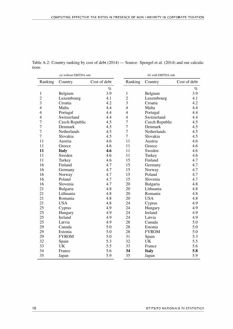
Finally, Table A.2 ranks EU member states, FYROM and Turkey as well as Norway, Switzerland,Canada, Japan and the United States on the basis of the cost of debt. Taking into account the EBITDArule Italy slips from the 11th position at the bottom of the ranking.

Table A.1: ETRs by assets and source of finance — with and without the EBITDA rule (2014)

Cost of capital Retained earnings Debt Debt Mean (all sources of finance)EMTR New equity without with without withEATR EBITDA EBITDA EBITDA EBITDA% rule rule rule rule

Buildings 6.2 5.0 6.6 5.8 5.819.3 -0.5 24.3 13.6 13.627.6 23.4 23.5 26.2 26.2

Intangibles 4.6 3.4 3.9 4.2 4.2-8.6 -47.5 -29.3 -19.0 -19.022.1 17.9 17.9 20.7 20.7

Machinery 6.3 5.1 5.2 5.9 5.920.8 1.9 3.1 15.3 15.328.0 23.8 23.8 26.6 26.6

Financial 6.2 5.0 6.9 5.8 6.0assets 18.7 0.0 27.1 13.3 16.2

24.8 20.6 21.9 23.4 23.4Inventory 5.7 4.5 6.5 5.3 5.6

12.4 -11.3 23.0 5.7 10.125.9 21.7 23.0 24.5 24.5

Mean (all assets) 5.8 4.6 5.8 5.4 5.413.8 -8.8 13.9 7.4 7.425.7 21.5 21.5 24.3 24.3



Table A.2: Country ranking by cost of debt (2014) — Source: Spengel et al. (2014) and our calcula-tions

(a) without EBITDA rule

Ranking Country Cost of debt

%1 Belgium 3.92 Luxembourg 4.13 Croatia 4.24 Malta 4.44 Portugal 4.44 Switzerland 4.47 Czech Republic 4.57 Denmark 4.57 Netherlands 4.57 Slovakia 4.511 Austria 4.611 Greece 4.611 Italy 4.611 Sweden 4.611 Turkey 4.616 Finland 4.716 Germany 4.716 Norway 4.716 Poland 4.716 Slovenia 4.721 Bulgaria 4.821 Lithuania 4.821 Romania 4.821 USA 4.825 Cyprus 4.925 Hungary 4.925 Ireland 4.925 Latvia 4.929 Canada 5.029 Estonia 5.029 FYROM 5.032 Spain 5.333 UK 5.534 France 5.635 Japan 5.9

(b) with EBITDA rule

Ranking Country Cost of debt

%1 Belgium 3.92 Luxembourg 4.13 Croatia 4.24 Malta 4.44 Portugal 4.44 Switzerland 4.47 Czech Republic 4.57 Denmark 4.57 Netherlands 4.57 Slovakia 4.511 Austria 4.611 Greece 4.611 Sweden 4.611 Turkey 4.615 Finland 4.715 Germany 4.715 Norway 4.715 Poland 4.715 Slovenia 4.720 Bulgaria 4.820 Lithuania 4.820 Romania 4.820 USA 4.824 Cyprus 4.924 Hungary 4.924 Ireland 4.924 Latvia 4.928 Canada 5.028 Estonia 5.028 FYROM 5.031 Spain 5.332 UK 5.533 France 5.634 Italy 5.835 Japan 5.9



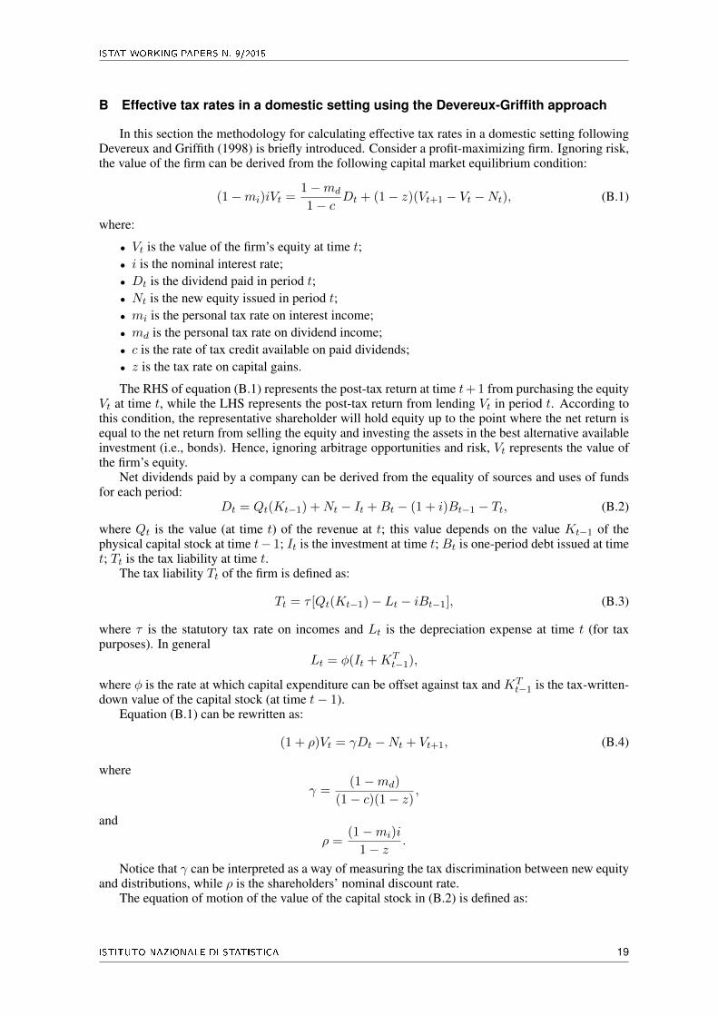
B Effective tax rates in a domestic setting using the Devereux-Griffith approach

In this section the methodology for calculating effective tax rates in a domestic setting followingDevereux and Griffith (1998) is briefly introduced. Consider a profit-maximizing firm. Ignoring risk,the value of the firm can be derived from the following capital market equilibrium condition:

(1−mi)iVt =1−md

1− cDt + (1− z)(Vt+1 − Vt −Nt), (B.1)

where:

• Vt is the value of the firm’s equity at time t;• i is the nominal interest rate;• Dt is the dividend paid in period t;• Nt is the new equity issued in period t;• mi is the personal tax rate on interest income;• md is the personal tax rate on dividend income;• c is the rate of tax credit available on paid dividends;• z is the tax rate on capital gains.

The RHS of equation (B.1) represents the post-tax return at time t+ 1 from purchasing the equityVt at time t, while the LHS represents the post-tax return from lending Vt in period t. According tothis condition, the representative shareholder will hold equity up to the point where the net return isequal to the net return from selling the equity and investing the assets in the best alternative availableinvestment (i.e., bonds). Hence, ignoring arbitrage opportunities and risk, Vt represents the value ofthe firm’s equity.

Net dividends paid by a company can be derived from the equality of sources and uses of fundsfor each period:

Dt = Qt(Kt−1) +Nt − It +Bt − (1 + i)Bt−1 − Tt, (B.2)

where Qt is the value (at time t) of the revenue at t; this value depends on the value Kt−1 of thephysical capital stock at time t− 1; It is the investment at time t; Bt is one-period debt issued at timet; Tt is the tax liability at time t.

The tax liability Tt of the firm is defined as:

Tt = τ [Qt(Kt−1)− Lt − iBt−1], (B.3)

where τ is the statutory tax rate on incomes and Lt is the depreciation expense at time t (for taxpurposes). In general

Lt = φ(It +KTt−1),

where φ is the rate at which capital expenditure can be offset against tax and KTt−1 is the tax-written-

down value of the capital stock (at time t− 1).Equation (B.1) can be rewritten as:

(1 + ρ)Vt = γDt −Nt + Vt+1, (B.4)

where

γ =(1−md)

(1− c)(1− z),

and

ρ =(1−mi)i

1− z.

Notice that γ can be interpreted as a way of measuring the tax discrimination between new equityand distributions, while ρ is the shareholders’ nominal discount rate.

The equation of motion of the value of the capital stock in (B.2) is defined as:



Kt = (1 + π)(1− δ)Kt−1 + It,

where π is the nominal annual inflation rate and δ is the one-period economic depreciation (due towear and tear).

Proceeding recursively, from Equation (B.4) the value of the firm at time t is derived:

(1 + ρ)Vt =+∞∑s=0

γDt+s −Nt+s

(1 + ρ)s. (B.5)

In order to compute the effective tax rates, consider a perturbation of the capital stock in oneperiod. At time t investment It, and hence capital stock Kt, increase by one unit. At time t + 1 thefirm goes back to its original condition, selling the piece of physical capital purchased at time t andcontextually repaying the debt or buying back the equity at the original price. Because of the shock13 ∆Qt+1 = (1 + π)(p + δ), where p represents the financial return of the new investment due tothe shock at time t. The firm chooses to finance the investment in period t through a combination ofsources of funds: retained earnings, new equity and debt.

By (B.5) it is straightforward that Rt is given by

Rt := (1 + ρ)∆Vt =

+∞∑s=0

γ∆Dt+s −∆Nt+s

(1 + ρ)s. (B.6)

Independently of the firm’s source of finance, we have that ∆It = 1, ∆Kt = 1, ∆Qt = 0,∆Tt = −τ∆Lt and hence, by Equation (B.2), ∆Dt = ∆Bt+∆Nt−1+τ∆Lt and γ∆Dt−∆Nt =−γ + γ∆Bt −∆Nt(1− γ) + γτ∆Lt.

At time t + 1: ∆Nt+1 = −∆Nt, ∆Bt+1 = 0, ∆It+1 = −(1 + π)(1 − δ), ∆Kt+1 = 0,∆Qt+1 = (1 + π)(p + δ), ∆Tt+1 = τ(1 + π)(p + δ) − τi∆Bt − τ∆Lt+1 and hence ∆Dt+1 =(1 + π)(p+ δ)(1− τ) + (1 + π)(1− δ)−∆Nt + ∆Bt(−1− i(1− τ)) + τ∆Lt+1. The second term(s = 1) of the series in Equation (B.6) can then be re-written as:

γ

1 + ρ((1 + π)(p+ δ)(1− τ) + (1 + π)(1− δ) + ∆Bt(−1− i(1− τ))) +

+1

1 + ρ∆Nt(1− γ) +

γ

1 + ρτ∆Lt+1.

Let us consider the terms of the series in Equation (B.6) when s ≥ 2. ∆Nt+s = 0, ∆Bt+s = 0,∆It+s = 0, ∆Kt+s = 0, ∆Qt+s = 0, ∆Tt+s = −τ∆Lt+s and hence ∆Dt+s = τ∆Lt+s. Thus thes-term of the series can be re-written as

γ∆Dt+s

(1 + ρ)s=γτ∆Lt+s(1 + ρ)s

.

Putting everything together we get

Rt = RREt + Ft, (B.7)

whereRREt is the rent attributable to investments financed by retained earnings and Ft is the additional

cost of raising external finance. In particular, as in (Devereux and Griffith, 1998, Equations 3.9, 3.10),

RREt := −γ(1−A) +

γ

1 + ρ((1 + π)(p+ δ)(1− τ) + (1 + π)(1− δ)(1−A)), (B.8)

Ft := γ∆Bt

(1− 1 + i(1− τ)

1 + ρ

)− (1− γ)∆Nt

(1− 1

1 + ρ

), (B.9)

13 Please, be aware that ∆ always indicates the difference between the value of the variable in the presence and in the absence of aperturbation in the capital stock and not a difference between consecutive time periods.



where A is the net present value of depreciation allowances per unit of investment.The tax-written-down value of the capital stock depends on the method applied for computing

depreciation expenses: declining balance, straight line or other special provisions. For instance in thecase of exponential, or declining balance, depreciation we have that KT

t varies according to

KTt = (1− φ)(KT

t−1 + It).

In this case

A = τφ

(1 +

1− φ1 + ρ

+(1− φ)2

(1 + ρ)2+ · · ·

)=τφ(1 + ρ)

ρ+ φ.

In the case of straight line depreciation:

A = τφ

(1 +

1

1 + ρ+ · · ·+ 1

(1 + ρ)s−1

)+

τλ

(1 + ρ)s=τφ(1 + ρ)

ρ

(1− 1

(1 + ρ)s

)+

τλ

(1 + ρ)s,

(B.10)where s :=

[1φ

]is the integer part of 1

φ and λ := 1− sφ.

It is convenient to single out the depreciation allowances from RREt :

RREt = RRE

t +RAt ,

where RAt is the net present value of depreciation allowances taking into account the tax benefit

over the whole life of the investment good less what is lost due to the disinvestment, while RREt =

RREt − RA

t . In particular RAt includes both the fiscal allowances related to the investment at time t

and the (negative) fiscal allowances due to the disinvestment at time t+ 1. In particular

RREt := −γ +

γ

1 + ρ((1 + π)(p+ δ)(1− τ) + (1 + π)(1− δ)) , (B.11)

RAt = γτ

+∞∑s=0

∆Lt+s(1 + ρ)s

= γA

(1− (1 + π)(1− δ)

1 + ρ

). (B.12)

As conventional for this literature, Rt is computed using (B.7), reducing the possible combina-tions of financing the investment to three cases: through retained earnings, new equity, and debt. Thefinancial constraints with respect to the three strategies are summarized in the table below:

Table B.1: Financial constraints on investment according to different sources of finance

Ret. Earnings New Equity Debt

∆Bt 0 0 1− τ∆Lt∆Nt 0 1− τ∆Lt 0

Observe that if the investment is financed by retained earnings Ft is always zero, thusRt = RREt .If personal taxation is not considered then γ = 1 and ρ = i, therefore Ft = 0 also if the investment isfinanced by new equity.

By setting the post-tax economic rent Rt to zero and solving for p we get the minimum requiredrate of return, the so-called cost of capital, denoted by p̃

p̃ =1−A

(1− τ)(1 + π)[ρ+ δ(1 + π)− π]− Ft(1 + ρ)

γ(1− τ)(1 + π)− δ.

The EMTR is defined asp̃− hp̃

,



where h is the post tax real rate of return to the shareholder:

h =(1−mi)i− π

1 + π.

Let us call R∗t the pre-tax economic rent at time t. The EATR is defined as

EATR =R∗t −Rt

p(1+r)

. (B.13)

In a world without corporate and personal taxation (i.e., γ = 1, ρ = i, τ = 0, A = 0) by Equation(B.7) we get:

R∗t = −1 +1

1 + i((1 + π)(p+ δ) + (1 + π)(1− δ)) =

p− r1 + r

, (B.14)

where r is the real interest rate: (1 + r)(1 + π) = (1 + i). The value of the EATR now follows.



References

Altshuler, R. and Grubert, H. (2006). Governments and Multinational Corporations in the Race to theBottom. Tax Notes, 110(8).

Bilicka, K., Devereux, M., and Fuest, C. (2011). G20 Corporate tax ranking 2011. Saïd BusinessSchool, University of Oxford.

Blouin, J., Huizinga, H., Laeven, L., and Nicodème, G. (2014). Thin capitalization rules and multi-national firm capital structure. Working Paper 12/14 - International Monetary Fund.

Bresciani, V. and Giannini, S. (2003). Effective Marginal tax rates in Italy. Prometeia, Nota di lavoro2003-01:1–33.

Buettner, T., Overesch, M., Schreiber, U., and Wamser, G. (2012). The impact of thin-capitalizationrules on the capital structure of multinational firms. Journal of Public Economics, 96(11):930–938.

Buslei, H. and Simmler, M. (2012). The impact of introducing an interest barrier: evidence from theGerman corporation tax reform 2008. DIW Berlin Discussion Paper.

Devereux, M., Elschner, C., Endres, D., Spengel, C., Bartholmess, A., Dressler, D., Finke, K., Heck-emeyer, J., and Zinn, B. (2009). Effective Tax Levels using the Devereux/Griffith methodology.Project for the EU commission TAXUD/2008/CC/099 - Mannheim und Oxford.

Devereux, M. and Griffith, R. (1998). The taxation of discrete investment choices. Working Paper98/16 - Institute of fiscal studies.

Devereux, M. P. and Griffith, R. (2003). Evaluating tax policy for location decisions. InternationalTax and Public Finance, 10(2):107–126.

EEC (2001). Company taxation in the internal market. Commission staff working paper,(SEC1681):1–423.

Egger, P., Loretz, S., Pfaffermayr, M., and Winner, H. (2009). Firm-specific forward-looking effectivetax rates. International Tax and Public Finance, 16(6):850–870.

Haufler, A. and Runkel, M. (2012). Firms’ financial choices and thin capitalization rules undercorporate tax competition. European Economic Review, 56(6):1087–1103.

King, M. and Fullerton, D. (1984). The taxation of income from capital: a comparative study of theUnited States, the United Kingdom, Sweden and West Germany. The Chicago University Press.

Klemm, A. (2012). Effective average tax rates for permanent investment. Journal of Economic andSocial Measurement, 37:253–264.

OECD (1991). Taxing Profits in a Global Economy — Domestic and International Issues. OECD.

OECD (2013). Supporting Investment in Knowledge Capital, Growth and Innovation. OECD Pub-lishing – http: // dx. doi. org/ 10. 1787/ 9789264193307-en .

OECD (2015). BEPS ACTION 4: Interest deductions and other financial payments. OECD PublicDiscussion Draft.

Spengel, C., Endres, D., Finke, K., and Heckemeyer, J. (2014). Effective Tax Levels using the Dev-ereux/Griffith methodology. Project for the EU commission TAXUD/2013/CC/120 - Mannheim.

Suzuki, M. (2014). Corporate effective tax rates in Asian countries. Japan and the World Economy,29(0):1 – 17.

Webber, S. (2010). Thin capitalization and interest deduction rules: a worldwide survey. Tax notesinternational, 60(9):683–708.


http://dx.doi.org/10.1787/9789264193307-en


Weichenrieder, A. J. and Windischbauer, H. (2008). Thin-capitalization rules and company responses-experience from german legislation. CESifo Working Paper Series.

Zangari, E. (2009). Gli effetti della riforma della tassazione societaria in Italia sulle preferenze fi-nanziarie e sulle scelte di investimento delle imprese. Politica Economica, XXV(2):147–183.


computing effective tax rates in presence of non … · computing effective tax rates in presence...

Documents