required rates of return for corporate investment appraisal in the presence of growth...
TRANSCRIPT

Hirst, I. and Danbolt, J. and Jones, E. (2008) Required rates of return for corporate investment appraisal in the presence of growth opportunities. European Financial Management 14(5):pp. 989-1006.
http://eprints.gla.ac.uk/4644/ 21th October 2008
Glasgow ePrints Service https://eprints.gla.ac.uk

Required Rates of Return for Corporate Investment Appraisal in the Presence of Growth Opportunities Ian R. C. Hirst Department of Accountancy and Finance, School of Management and Languages, Heriot-Watt University, Edinburgh, EH14 4AS, Scotland, UK e-mail: [email protected] Jo Danbolt Department of Accounting and Finance, University of Glasgow, Glasgow, G12 8LE, Scotland, UK e-mail: [email protected] Eddie Jones Management School and Economics, University of Edinburgh, Edinburgh, EH8 9JY, Scotland, UK e-mail: [email protected]
Abstract
Traditional methods of estimating required rates of return overstate hurdle rates in the presence of growth opportunities. We attempt to quantify this effect by developing a simple model which: (i) identifies those companies that have valuable growth opportunities; (ii) splits the value of shares into ‘assets-in-place’ and ‘growth opportunities’; and (iii) splits the equity β into β for ‘assets-in-place’ and ‘growth opportunities’. We find growth opportunities for UK companies over the 1990-2004 period to average 33% of equity value. Incorporating the effect of growth opportunities, the average cost of capital for investment purposes falls by 1.1 percentage points. Keywords: Cost of capital, Beta, Growth opportunities, Assets-in-place JEL Classification: G31 Acknowledgements The authors would like to thank the anonymous referee, John Doukas, Mark Aleksanyan, Joe Hillier, Brian Nichols, Graham Partington, Antonios Siganos and participants at the Financial Management Association Annual Meeting (Siena, 2005), the Multinational Finance Society Annual Conference (Edinburgh, 2006), the European Financial Management Association Annual Conference (Madrid, 2006) and seminars at Glasgow Caledonian University and Glasgow University for helpful comments on earlier versions of this paper. The normal caveat applies.

1. Introduction
This paper builds on an argument that was first proposed by Myers and Turnbull (1977).
They note that the market value of the firm is made up of: (i) The present value of cash
flows from assets-in-place, and (ii) the present value of growth opportunities. They
further note that growth opportunities have option-like characteristics, and that this has
implications for rates of return that incorporate the measurement of systematic risk. They
conclude:
“The risk (β) of an option is not the same as the risk of the asset the option is
written on. Usually it is greater. If so, the larger the option value relative to the
value of assets-in-place, the greater is the systematic risk of the firm’s stock.
Thus the systematic risk of the firm’s stock is an overestimate of the beta for
tangible assets, and a rate of return derived from common stock β’s will be an
overestimate of the appropriate hurdle rate for capital investment whenever firms
have valuable growth options. The practical and theoretical difficulties created by
this phenomenon are obvious”. (Myers and Turnbull, 1977, p. 332).
This paper attempts to tackle these ‘practical and theoretical difficulties’. Our main
contribution is to develop a simple model, based on standard pieces in the toolkit of
financial theory, to split the β of a company’s shares into the two elements of ‘assets-in-
place β’ and ‘growth opportunities β’. We also adjust the cost of capital for the presence
of growth opportunities, and explore the properties of the model by applying it to a large
sample of UK companies over the 1990-2004 period.
Myers and Turnbull’s argument, as well as our model, suggests growth opportunities
should affect required rates of return whichever investment appraisal method is chosen.
To illustrate the magnitude of the growth opportunities effect, we look specifically at the
2

change in the value of the weighted average cost of capital (WACC) when growth is
taken into account.
In light of Myers and Turnbull’s analysis, it can be seen that the traditional method of
calculating WACC for investment in new assets is doubly flawed. Not only does it use
the wrong β for equity committed to new assets; it also uses the wrong weights when
combining the costs of debt and equity. If debt is supported by assets-in-place, the weight
given to equity should be based solely on the market value of equity derived from assets-
in-place, omitting the market value of the company’s growth opportunities.
From an initial sample of 5,059 firm-year observations, we are able to estimate the value
of growth opportunities for 3,715 cases. However, some of these cases yield negative
estimates for the value of growth opportunities. Our model applies to those cases in
which companies have valuable growth opportunities. Assuming an equity risk premium
of 6%, we identify valuable growth opportunities in 69% of the cases to which we can
apply the model (and 51% of the whole dataset). For these 2,571 cases, we find that
growth opportunities account, on average, for 33% of equity value. Adjusting WACC for
the presence of valuable growth opportunities lowers the hurdle rate for new investments
on average by just over one percentage point. The adjustment is larger for companies with
higher levels of growth opportunities, rising to just over two percentage points for the
decile of observations with the highest levels of growth opportunities.
The remainder of the paper is organised as follows: In section 2 we review relevant prior
work, while in section 3 we develop and solve the set of equations used in our model for
splitting the equity beta. Section 4 develops the model for adjusting the cost of capital for
the presence of growth opportunities. In section 5 we apply the model to a large sample
3
of UK listed companies, while in section 6 we explore some of the properties of the
model. The final section sets out our conclusions.
2. Literature and theoretical foundations
Recognition that share value is divided into assets-in-place and growth opportunities
dates back to Miller and Modigliani (1961).1 Kester (1984) demonstrates a practical
method of decomposing share prices into the value of assets-in-place and growth
opportunities, and a development of this model has been given prominence in Brealey
and Myers (1991 and subsequent editions). On a per share basis (where the value of one
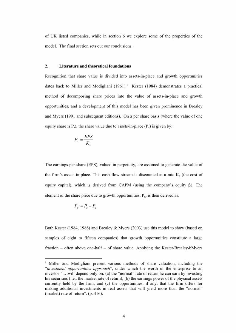
equity share is Ps), the share value due to assets-in-place (Pa) is given by:
sa K
EPSP =
The earnings-per-share (EPS), valued in perpetuity, are assumed to generate the value of
the firm’s assets-in-place. This cash flow stream is discounted at a rate Ks (the cost of
equity capital), which is derived from CAPM (using the company’s equity β). The
element of the share price due to growth opportunities, Pg, is then derived as:
asg PPP −=
Both Kester (1984, 1986) and Brealey & Myers (2003) use this model to show (based on
samples of eight to fifteen companies) that growth opportunities constitute a large
fraction – often above one-half – of share value. Applying the Kester/Brealey&Myers
1 Miller and Modigliani present various methods of share valuation, including the “investment opportunities approach”, under which the worth of the enterprise to an investor “…will depend only on: (a) the “normal” rate of return he can earn by investing his securities (i.e., the market rate of return); (b) the earnings power of the physical assets currently held by the firm; and (c) the opportunities, if any, that the firm offers for making additional investments in real assets that will yield more than the “normal” (market) rate of return”. (p. 416).
4

model to larger samples, Danbolt et al. (2002)2 find growth opportunities on average to
account for 56% of firm value based on a sample of 2,010 firm-years for large UK
companies, while Andrés-Alonso et al. (2006), applying a variant of the
Kester/Brealey&Myers model to a sample of 391 high-tech companies listed in OECD
markets, find the value of growth opportunities to average more than 75% of firm value.
However, the Kester/Brealey&Myers method, by valuing the assets-in-place at a discount
rate based on equity β, ignores the central insight of Myers and Turnbull. Thus, while the
method is a well established technique for measuring growth opportunities, it is not
satisfactory for our purpose. To develop the Myers and Turnbull analysis, we require a
model which measures not just values for ‘assets-in-place’ and ‘growth opportunities’,
but also generates the β values associated with each component.
A number of papers have developed theoretical models of the impact of growth options
on share beta and the beta of assets in place (e.g., Miles, 1986; Pindyck, 1988; Chung and
Charoenwong, 1991; Chung and Kim, 1997). However, these papers rely on variables
that are not readily observable, and the models cannot easily be applied to real firms.
A paper by Ben-Horim and Callen (1989) is perhaps closest in method to the present
paper. They recommend the use of Tobin’s Q to estimate future growth opportunities.3
2 Danbolt et al. (2002) also provide a critical evaluation of the Kester/Brealey&Myers method. 3 A number of prior studies (e.g., Lang et al., (1989); Alexandrou and Sudarsanam, (2001)) have similarly used Tobin’s Q, or the Market-to-Book ratio, as a proxy for the level of growth opportunities. However, as these studies have not attempted to measure the level of growth opportunities, nor commented on the impact of growth opportunities on the cost of capital, a review of this strand of literature is beyond the scope of this paper.
5

They use the dividend discount model, as we shall do, and they demonstrate their model
by applying it to a major US corporation. However, Ben-Horim and Callen do not use an
asset-pricing model and are concerned only to measure the cost of equity capital defined
as the return expected by investors in the shares.
While prior studies have addressed the measurement of growth opportunities, they do not
– with the exception of Chung and Kim’s (1997) theoretical model – address Myers and
Turnbull’s (1977) central concern that the traditional method of calculating the cost of
capital based on equity β provides an overestimate of the appropriate hurdle rate for
companies with valuable growth opportunities. In this paper, we aim to address this gap
in the literature.
3. A model for splitting the equity β
The model is built on the following assumptions:
1. The company grows at a constant rate, g. This growth rate applies to the book value
of debt, equity and all categories of assets and liabilities. It also applies to cash flows,
earnings and dividends. Growth is value creating, and we assume new projects, like
existing projects, have positive NPV’s. Where do these valuable projects come from?
We assume, with Myers and Turnbull, that the acquisition of growth opportunities is
independent of the acquisition of real assets. We do not model the acquisition of
growth opportunities. We simply assume that the company initially holds a set of
future growth opportunities (with one ‘opportunity’ for each future year) on which its
future growth will be based. Investment is needed to generate cash-flows from
growth opportunities, but growth opportunities themselves are not acquired through
investment.
6

New projects are funded with the same mix of debt and equity as existing projects
and this gearing ratio remains constant throughout a project’s life. The dividend and
all variables growing at rate g are measured on a ‘per share’ basis. Growth is
measured in real terms. The Gordon (1959) dividend-discount model can therefore be
used to value the firm’s shares.
These assumptions create a simple and tractable model whose limitations must be
recognised. The company is on a fixed growth track and its growth opportunities are
not traditional growth options. They do not have all the characteristics that would be
predicted by a standard option pricing model. Growth is expected to continue in
perpetuity. Although the company uses part of its growth opportunities every year,
the value of its overall set of growth opportunities is not diminished because its future
stream of profitable investments has drawn closer and hence become more valuable.
Although companies often have long-term growth opportunities, we recognise that
perpetual growth is an extreme case.
2. Asset prices are set using the standard capital asset pricing model (CAPM).
3. As the company grows, its new investment projects have the same characteristics as
its existing projects. We assume that newly acquired assets have the same beta, βa, as
the stock of existing assets. Thus the asset beta remains constant when new assets are
acquired. Similarly, we assume that the β of the growth opportunity which is used in
any year is the same as the β of the remaining portfolio of growth opportunities.
Hence, the growth opportunities beta, βg, remains constant when investment takes
place. At the point when investment takes place, the growth opportunity plus the
(book) value of the equity investment needed to implement it are put together to
7

become the new asset-in-place. Hence the β of assets-in-place (βa) is the weighted
average of the β of the growth opportunity (βg) and the β of the cash investment (βc).
The β of cash is zero.
4. The company’s debt is risk free and the book value of debt is equal to its market
value. Our model is based on the proposition that corporate debt capacity derives
from cash generating assets.4 Specifically, we assume that all debt is associated with
assets-in-place and that growth opportunities support no debt. Given these
assumptions and a constant debt-equity ratio, the level of debt plays no part in the
model for the derivation of the two betas. However, corporate debt will be relevant
when using the β’s to derive corporate required rates of return.
We use the following definitions. The variables in bold are those we seek to estimate,
while those in normal typeface are assumed to be directly observable or measurable:
D0 The annual dividend per share, assumed to be paid just prior to the
accounting year-end. (We obtain the data for the empirical analysis from
Datastream).
D1 The next annual dividend per share, due to be paid one year from the current
date.
Ps The share price as at the accounting year end.
Pa The component of the share price attributable to assets-in-place.
Pg The component of the share price attributable to growth opportunities.
E The accounting year end book value of equity (per share).
Ks Investors’ required rate of return on the firm’s shares.
4 This proposition has some support in the standard finance literature. See e.g., Brealey and Myers (2003): “Normally the firm’s optimal debt level increases as its assets expand…”. (p. 552).
8

Ka Investors’ required rate of return on equity funds used in the firm’s assets-in-
place.
Kf The risk free rate of interest. (We proxy this by the yield on long-term
government bonds).
Kg Investors’ required rate of return on the component of the share price
justified by growth opportunities.
Km The expected return on the market portfolio. (We take the equity risk
premium as given).
βs The beta of the firm’s shares.
βa The beta of the equity associated with the firm’s assets-in-place.5
βg The beta associated with the market value of the firm’s future growth
opportunities.
Our objective is to show how, based on our assumptions, the other variables can be
calculated from the six observed variables. Equations linking the variables are given
below.
From CAPM, we can calculate the required rate of return on the firm’s equity as follows:
)( fmsf KKK −+= βsK (1)
The constant growth, dividend discount model, gives a value for the share as:
g-KD
s
1=sP (2)
5 Note we are using the term beta of assets-in-place to refer to the beta of equity used (alongside debt) to finance assets-in-place. It is not an ‘asset beta’ created by ungearing an equity beta.
9

Since the dividend grows in proportion to the other dimensions of the company, next
year’s dividend can be estimated as:
)1(0 gD1 += D (3)
The price of the share is made up of the assets-in-place and the growth opportunities
components:
ga PP +=sP (4)
The firm could decide to abandon its growth opportunities. This would not be a value
maximising decision, but it is a theoretical possibility. The ‘price’ of taking up the
growth opportunities next year is E*g (i.e., the company grows its equity base at a rate
g). If the growth opportunities were abandoned, the dividend would be increased by this
amount. The expectation for this new level of dividend is that it would remain constant
(subject to normal business risk) and can be valued as a level perpetuity discounted at the
assets-in-place rate:
a
1a K
gDP
*E+= (5)
Note that the logic of this equation only works when growth opportunities are non-
negative. Growth opportunities have option-like characteristics. They could,
hypothetically, be abandoned and the company could carry on at its existing scale and
profitability. If an equivalent ‘contraction opportunity’ or ‘contraction option’ existed it
would never be exercised. The model is asymmetric. It can be applied to corporate
growth but it cannot be applied to firms that are shrinking in scale. This asymmetry is a
general characteristic of the ‘growth opportunities’ literature. Since Myers and Turnbull’s
observation relates specifically to companies that possess valuable growth opportunities,
this feature of the model is not a problem for our purpose.
10

The required rate of return for assets-in-place is derived, by way of CAPM, from the beta
of assets-in-place:
)( fmf KKK −+= aa βK (6)
Given that a share is effectively a portfolio composed of the assets-in-place and the
growth opportunities, the share beta will be a weighted average of the betas of the two
components:
gg
aa β
PβP
sss PP
+=β (7)
At the point in time when a growth opportunity is converted into an asset in place, the β
of the ‘package’ (the growth opportunity plus the equity funding (cash) needed for
conversion) is equal to the β of the newly created asset-in-place. We treat the ‘package’
as a portfolio of two assets, and note that the β of cash (βc) is zero.
The value of assets-in-place (Pa) exceeds the book value of equity (E) by the NPV of
current projects (the assets-in-place). From our assumptions, the ratio of NPV (for the
growth opportunity) to associated equity is the same at the point of investment as
throughout the rest of the project’s life. In addition, this ratio is the same for all the
projects that make up the company’s assets-in place. We have already argued that the β
of assets-in-place (βa) will be the weighted average of the β of growth opportunities (βg)
and the β of the cash needed to realise the opportunities.
What are the weights in this relationship? When the investment takes place, the total
value of the new asset-in-place is made up of the amount of equity (cash) invested plus
11

the value of the ‘opportunity’ (which is the investment’s NPV). The proportion of the
value that comes from the ‘opportunity’ is therefore:
placeinassetsnewofValueinvestmentequityofValueplaceinassetsnewofValue
−−−−−
From our assumptions, this proportion remains the same throughout the life of any project
and is the same for all projects undertaken by the firm. The proportion can therefore be
written as:
placeinassetsallofValueinvestmentequitycompanyallofvalueBookplaceinassetsallofValue
−−−−−
Or, expressed on a per share basis:
a
a
PP E−
Hence
cβEE
ag
a
aa P
βP
Pβ +−
=
Recognising that βC is zero, this simplifies to:
aa
ag β
PPβ
E-= (8)
This has given us a set of eight equations, and eight unknown variables: Pa, Pg, g, D1, Ks,
Ka, βa and βg. The nature of the eight equations is such that the system can be solved
relatively simply by a process of substitution.
12
4. Adjusting the cost of capital
When a company invests in new assets-in-place, the appropriate required rate of return
must – as argued by Myers and Turnbull (1977) – be based on the risk of assets-in-place.
For the equity element of funding, this is measured by the beta for assets-in-place (βa) and
not the beta for the share (βs). The set of equations in the previous section provides a
means of estimating βa. With this, we use CAPM to adjust the cost of equity capital from
that for the whole share (Ks) to the cost of equity capital for assets-in-place (Ka). The
equity beta of assets-in-place would be useful whether project appraisal used the
weighted average cost of capital (WACC), adjusted present value (APV) or project-
specific rates. However, for illustrating the impact of adjusting the required rate of return
for corporate investment appraisal in the presence of growth opportunities, we will
concentrate on the adjustment to WACC.
The traditional WACC not only uses an inappropriate cost of equity capital (Ks rather
than Ka), but also inappropriate weights of debt and equity. In calculating the cost-of-
capital for acquiring new assets, these should be the proportions used for financing new
(and existing) assets. In our model these proportions are derived from the whole of the
company’s debt and the equity market value of assets-in-place (Pa rather than Ps).
It should be noted that in the model for splitting the equity β outlined above, all growth
rates, interest rates and required returns are real rates. However, WACC is not only a
nominal rate by convention, but the ‘after tax’ adjustment for the cost of debt logically
relates to the nominal cost of debt. We therefore move in the calculations that follow
from real to nominal interest rates. The costs of equity for both conventional and adjusted
WACC simply rise by the level of forecast inflation – i.e., we replace the rate on index-
linked gilts by the rate on nominal gilts in the CAPM calculations. For the cost of debt we
13
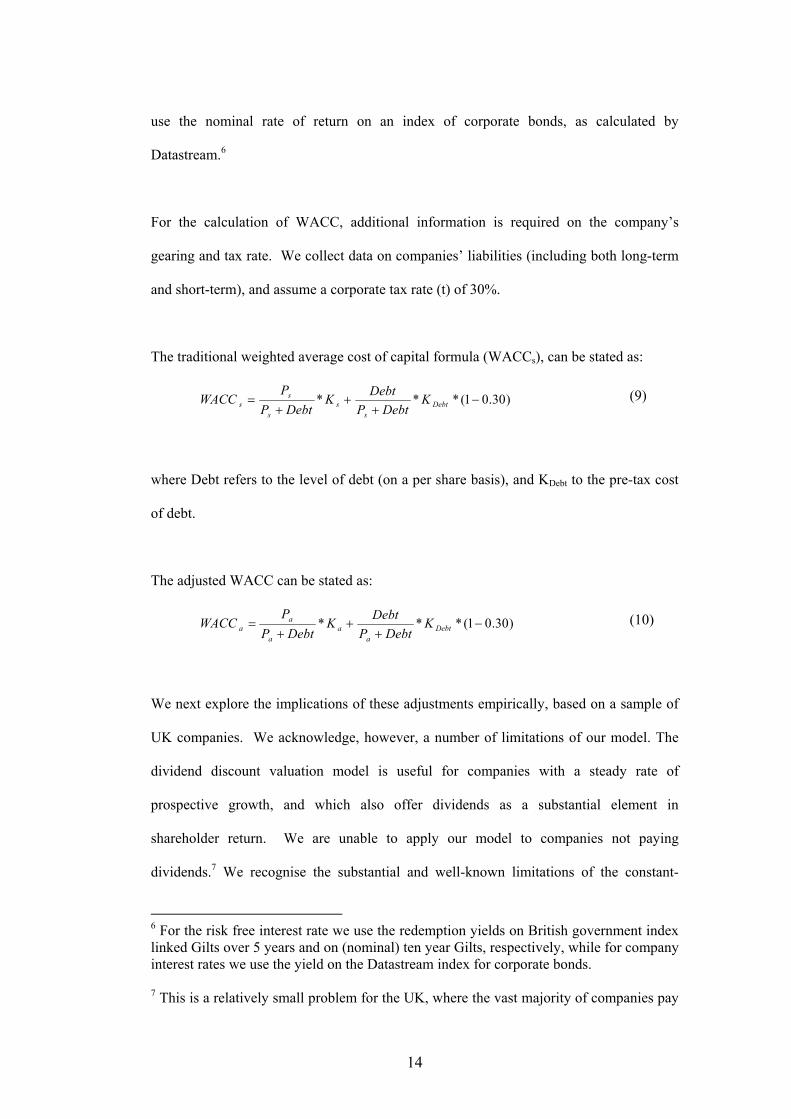
use the nominal rate of return on an index of corporate bonds, as calculated by
Datastream.6
For the calculation of WACC, additional information is required on the company’s
gearing and tax rate. We collect data on companies’ liabilities (including both long-term
and short-term), and assume a corporate tax rate (t) of 30%.
The traditional weighted average cost of capital formula (WACCs), can be stated as:
)30.01(*** −+
++
= Debts
ss
ss K
DebtPDebtK
DebtPP
WACC (9)
where Debt refers to the level of debt (on a per share basis), and KDebt to the pre-tax cost
of debt.
The adjusted WACC can be stated as:
)30.01(*** −+
++
= Debta
aa
aa K
DebtPDebtK
DebtPP
WACC (10)
We next explore the implications of these adjustments empirically, based on a sample of
UK companies. We acknowledge, however, a number of limitations of our model. The
dividend discount valuation model is useful for companies with a steady rate of
prospective growth, and which also offer dividends as a substantial element in
shareholder return. We are unable to apply our model to companies not paying
dividends.7 We recognise the substantial and well-known limitations of the constant-
6 For the risk free interest rate we use the redemption yields on British government index linked Gilts over 5 years and on (nominal) ten year Gilts, respectively, while for company interest rates we use the yield on the Datastream index for corporate bonds. 7 This is a relatively small problem for the UK, where the vast majority of companies pay
14

growth dividend discount model and of accounting measurements of assets and equity in
place.
5. Applying the model
To apply the model, we use data for the UK Financial Times All-Share constituent
companies over a fifteen-year period from January 1990 to December 2004. We are able
to obtain the accounting and market data from Datastream, and match this with beta
estimates from Dimson and Marsh’s Risk Measurement Service, for a sample of 5,059
firm-years. We obtain interest rate data from Datastream. Our model assumes
knowledge of the equity risk premium, and in the calculations that follow we assume this
to be 6%, which is towards the middle of the estimates put forward in the literature
(Dimson et al., 2003).
Since our model assumes a constant rate of growth for all the firm’s basic metrics, we
have to exclude cases with zero or negative value of equity (143 cases), with zero
dividends (571 cases), and where the book value of equity exceeds the share price (630
cases)8, leaving a sample of 3,715 firm-years for which we can calculate the value of
growth opportunities (Sample B), as detailed in Table 1.
Table 1 about here
substantial dividends. In their study of dividend payments in the UK during the 1990s, Renneboog and Trojanowski (2005) found 85% of listed companies to pay dividends, with dividends averaging 3.1% of market capitalisation, or 20.3% of earnings before interest and tax. Share repurchases were relatively uncommon, on average used by less than 6% of UK companies. These firms also tended to pay substantial dividends. Share repurchases averaged only 0.4% of market capitalisation, or 2.3% of EBIT. 8 In the model, this would imply that existing projects have negative NPV and no company would want to grow through scaling-up under these circumstances.
15
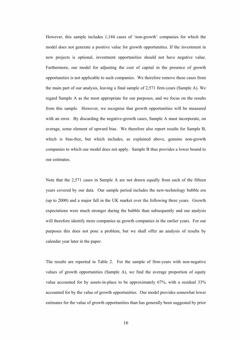
However, this sample includes 1,144 cases of ‘non-growth’ companies for which the
model does not generate a positive value for growth opportunities. If the investment in
new projects is optional, investment opportunities should not have negative value.
Furthermore, our model for adjusting the cost of capital in the presence of growth
opportunities is not applicable to such companies. We therefore remove these cases from
the main part of our analysis, leaving a final sample of 2,571 firm-years (Sample A). We
regard Sample A as the most appropriate for our purposes, and we focus on the results
from this sample. However, we recognise that growth opportunities will be measured
with an error. By discarding the negative-growth cases, Sample A must incorporate, on
average, some element of upward bias. We therefore also report results for Sample B,
which is bias-free, but which includes, as explained above, genuine non-growth
companies to which our model does not apply. Sample B thus provides a lower bound to
our estimates.
Note that the 2,571 cases in Sample A are not drawn equally from each of the fifteen
years covered by our data. Our sample period includes the new-technology bubble era
(up to 2000) and a major fall in the UK market over the following three years. Growth
expectations were much stronger during the bubble than subsequently and our analysis
will therefore identify more companies as growth companies in the earlier years. For our
purposes this does not pose a problem, but we shall offer an analysis of results by
calendar year later in the paper.
The results are reported in Table 2. For the sample of firm-years with non-negative
values of growth opportunities (Sample A), we find the average proportion of equity
value accounted for by assets-in-place to be approximately 67%, with a residual 33%
accounted for by the value of growth opportunities. Our model provides somewhat lower
estimates for the value of growth opportunities than has generally been suggested by prior
16

studies. Still, they account for a significant proportion of equity value for the majority of
companies, suggesting that the impact of adjusting the cost of capital in the light of such
growth opportunities may be non-trivial.
Table 2 about here
Our model requires adjustment to both weights and costs of equity in the WACC
calculation. The decomposition of the equity β gives us a β for assets-in-place (βa)
averaging 0.82 compared to βs of 0.97. The application of our model also results in a
reduced average weighting for the equity component in the company capital structure (from
Ws of 0.83 to Wa of 0.78), leading to a reduction in the average nominal cost of equity
capital (from Ks of 12.3% to Ka of 11.5%). The impact of these recalculations is to move
from an average traditional WACC of 11.1% to an adjusted WACC of 10.0% – a reduction
of almost 1.1 percentage points – when the cost of equity capital is calculated using our
model.
Our model has assumed that company investments convert a pre-owned growth
opportunity into a profitable asset-in-place. The adjusted WACC is appropriate for this
specific situation. The table, however, gives other information that might be relevant. If
a company could purchase growth opportunities on their own (a possibility that has not
formed part of our model), the appropriate required return would be based on the risk of
growth opportunities (βg). In the specific case where the company was making a
corporate acquisition and the target company’s mix of growth opportunities and assets-in-
place exactly matched its own, then traditional WACC would give the appropriate rate.
As explained above, the results for Sample A in Table 2 contain some element of upward
bias, and we therefore also report results for Sample B. The mean value of growth
17

opportunities for Sample B is naturally lower at 19% of firm value. So is the mean
adjustment to the cost of capital at 0.4 percentage points. However, given that our model,
and Myers and Turnbull’s insight, apply only to companies with valuable growth
opportunities, we caution against reading too much into the Sample B results.
6. Properties of the model and sensitivity analyses
The results reported in Table 2 are based on averages. We next explore: (i) the properties
of growth opportunities over time; and (ii) the sensitivity of the WACC adjustment to the
level of growth opportunities.9
6.1. Time-Series Variations in the Levels of Growth Opportunities.
The pooled results suggest growth opportunities on average account for 33% of share value.
However, our fifteen-year sample period includes periods of very different economic
climates, and we next explore the properties of our model estimates over the sample period.
As can be seen from Figure 1, the value of growth opportunities has varied significantly
over time. As the UK recovered from a recession in the early 1990s, the value of growth
opportunities increased and the proportion of firms with estimated negative values of
growth opportunities declined. However, the frequency of negative values of growth
opportunities once again rose with the bursting of the new-technology bubble. For the
companies with valuable growth opportunities (Sample A), the average level of growth
opportunities increased slowly during the 1990s, from 33% in 1990 to a peak of 39% in
9 We have also tested the sensitivity of our model to the assumed level of the equity risk premium. The number of firm-years for which we identify positive growth opportunities increases with the risk premium, and the adjustments to the cost of capital would also be somewhat higher assuming a higher equity risk premium. With a risk premium of 5% (7%), growth opportunities on average account for 30% (34%) of firm value, compared to 33% based on an assumed equity risk premium of 6%. While the mean adjustment to WACC amounts to 1.1 percentage points assuming a 6% equity risk premium (as reported in Table 2), this falls to 0.8 percentage points assuming a 5% risk premium, or rise to 1.3 percentage points assuming a 7% equity risk premium.
18
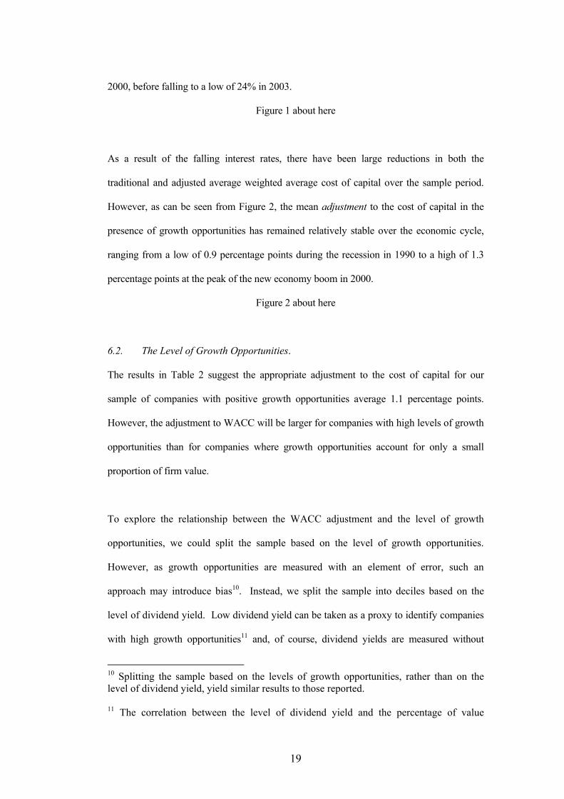
2000, before falling to a low of 24% in 2003.
Figure 1 about here
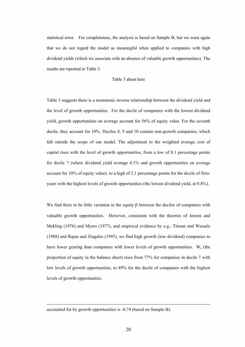
As a result of the falling interest rates, there have been large reductions in both the
traditional and adjusted average weighted average cost of capital over the sample period.
However, as can be seen from Figure 2, the mean adjustment to the cost of capital in the
presence of growth opportunities has remained relatively stable over the economic cycle,
ranging from a low of 0.9 percentage points during the recession in 1990 to a high of 1.3
percentage points at the peak of the new economy boom in 2000.
Figure 2 about here
6.2. The Level of Growth Opportunities.
The results in Table 2 suggest the appropriate adjustment to the cost of capital for our
sample of companies with positive growth opportunities average 1.1 percentage points.
However, the adjustment to WACC will be larger for companies with high levels of growth
opportunities than for companies where growth opportunities account for only a small
proportion of firm value.
To explore the relationship between the WACC adjustment and the level of growth
opportunities, we could split the sample based on the level of growth opportunities.
However, as growth opportunities are measured with an element of error, such an
approach may introduce bias10. Instead, we split the sample into deciles based on the
level of dividend yield. Low dividend yield can be taken as a proxy to identify companies
with high growth opportunities11 and, of course, dividend yields are measured without
10 Splitting the sample based on the levels of growth opportunities, rather than on the level of dividend yield, yield similar results to those reported. 11 The correlation between the level of dividend yield and the percentage of value
19
statistical error. For completeness, the analysis is based on Sample B, but we warn again
that we do not regard the model as meaningful when applied to companies with high
dividend yields (which we associate with an absence of valuable growth opportunities). The
results are reported in Table 3.
Table 3 about here
Table 3 suggests there is a monotonic inverse relationship between the dividend yield and
the level of growth opportunities. For the decile of companies with the lowest dividend
yield, growth opportunities on average account for 56% of equity value. For the seventh
decile, they account for 10%. Deciles 8, 9 and 10 contain non-growth companies, which
fall outside the scope of our model. The adjustment to the weighted average cost of
capital rises with the level of growth opportunities, from a low of 0.1 percentage points
for decile 7 (where dividend yield average 4.1% and growth opportunities on average
account for 10% of equity value), to a high of 2.1 percentage points for the decile of firm-
years with the highest levels of growth opportunities (the lowest dividend yield, at 0.8%).
We find there to be little variation in the equity β between the deciles of companies with
valuable growth opportunities. However, consistent with the theories of Jensen and
Mekling (1976) and Myers (1977), and empirical evidence by e.g., Titman and Wessels
(1988) and Rajan and Zingales (1995), we find high growth (low dividend) companies to
have lower gearing than companies with lower levels of growth opportunities. Ws (the
proportion of equity in the balance sheet) rises from 77% for companies in decile 7 with
low levels of growth opportunities, to 89% for the decile of companies with the highest
levels of growth opportunities.
accounted for by growth opportunities is -0.74 (based on Sample B).
20

In Table 3, conventionally measured WACC (WACCs) appears similar for companies
with valuable growth opportunities and firms with few or no growth opportunities. These
numbers, however, are potentially misleading. The highest growth observations in our
data set tend to come from the years prior to 2000 when interest rates were high. Our low
growth observations tend to come from the final years of our data, when interest rates
were substantially lower. To remove the influence of varying interest rates, the table also
shows the ‘WACC premium’ – the value of WACC less the nominal risk free interest rate
– both for conventional calculation and after Myers-Turnbull adjustment. Our discussion
will focus on this measure.
The conventional picture shows that high growth companies have a higher cost of capital
(measured by the WACC premium). They use more equity in their capital mix (78% at
decile 7 compared to 89% at decile 1), but their equity is still just as risky. Equity β is
similar across the deciles (0.94 for decile 7 and 0.98 for decile 1). The result is that the
conventional WACC premium rises from 4.1% for decile 7 to 5.1% for decile 1.
After Myers-Turnbull adjustment and with 100% equity finance for growth opportunities
the picture looks very different. For financing assets-in-place we find no tendency for
higher growth companies to use less gearing. This is a notable observation. The tendency
for growth companies to use low levels of gearing is widely recognised in the empirical
literature, with ‘Pecking order’ and ‘agency’ theories being offered as explanations. Our
results suggest an alternative possible explanation. The variability in overall gearing can
be fully explained by the proposition that growth opportunities are 100% equity financed.
High growth and lower growth companies appear in our analysis to use almost exactly the
same level of gearing in financing assets-in-place (77% at decile 7 and 79% at decile 1).
21

Table 3 also shows that the assets-in-place equity β is lower for companies with higher
growth prospects (0.94 for decile 7 and 0.70 for decile 1). The combined effect of the
lower β and the unchanged gearing is that the adjusted WACC premium is actually lower
for companies with higher growth potential. It falls from 4.0% for decile 7 to 3.1% for
decile 1. Without adjustment it rises from 4.1% to 5.1%. The adjusted numbers have
some intuitive appeal. Why should the hurdle rate be higher for asset investments by a
high-growth company than for a low-growth company? We might hypothesise that, other
factors equal, there is less risk in increasing a company’s stock of assets when the
business has an underlying tendency to grow than when it does not. The lower risk would
lead to a lower required return. After Myers-Turnbull adjustment the numbers are
consistent with this argument.
7. Conclusions
This paper is based on the well-established division of share value into growth
opportunities and assets-in-place. It has built on the insight of Myers and Turnbull (1977)
who showed that, in the presence of growth opportunities, the risk level of the company’s
assets will differ from the risk level of its shares. The required rate of return for asset
investment should be adjusted accordingly.
We have constructed a model, based on standard elements in finance theory, which splits
the equity β of a company into a growth opportunities element and an assets-in-place
element, and applied this model to a sample of 2,571 firm-year cases for UK companies
over the 1990-2004 period. Our results suggest (assuming an equity risk premium of 6
percentage points) that assets in place on average account for 67% of equity value,
leaving a residual 33% attributable to growth opportunities. Splitting the equity beta (βs,
which averages 0.97), we find the beta for assets-in-place (βa) to average 0.82 and the
22

beta of growth opportunities (βg) to be 1.48.
Using the traditional method for calculating hurdle rates, we find the cost of capital to be
generally higher for companies with high levels of growth opportunities. This finding is
closely linked to the lower gearing levels associated with high growth. However, after
making a Myers-Turnbull adjustment and assuming growth opportunities are 100%
equity financed, we find that companies across the growth spectrum use very similar
proportions of debt and equity to finance assets-in-place, and that high growth companies
have lower required returns for asset investments. The result follows from the observation
that the risk (β) associated with equity investment in new assets is lower for high growth
companies.
Controlling for the effect of growth opportunities lowers the cost of capital for investment
appraisal by an average of 1.1 percentage points. The adjustments increase with the level
of growth opportunities, rising from a low of 0.1 percentage points for the decile of firms
with the lowest positive values of growth opportunities, to 2.1 percentage points for the
decile with the highest levels of growth opportunities.
Analysis of the time-series properties of our model suggests both the level of growth
opportunities and the cost of capital has varied over the economic cycle. However, our
analysis suggests the adjustment to the cost of capital to take account of the effect of
growth opportunities has remained relatively stable over the sample period.
When they first recognised that growth opportunities had significant implications for the
required rates of return, Myers and Turnbull (1977) referred to the “practical and
theoretical difficulties” of making appropriate adjustments. Growth opportunities are
23

difficult to measure accurately, and the dividend discount model used here, like other
methods, has substantial limitations. Our analysis is, we believe, the first to try and
quantify the implications of Myers and Turnbull’s observations about growth
opportunities, and we have demonstrated that, for companies with large growth
opportunities, these implications are on a scale that has practical significance.
24

References
Alexandrou, G., and Sudarsanam, S., (2001), ‘Shareholder Wealth Effects of Corporate
Selloffs: Impact on Growth Opportunities, Economic Cycle and Bargaining
Power’, European Financial Management, Vol. 7, No. 2, pp. 237-258.
Andrés-Alonso, P., Azofra-Palenzuela, V., and Fuente-Herrero, G., (2006), ‘The Real
Options Component of Firm Value: The Case of the Technological Corporation’,
Journal of Business Finance & Accounting, Vol. 33, No. 1&2, pp. 203-219.
Ben-Horim, M., and Callen, J.L., (1989), ‘The Cost of Capital, Macaulay's Duration, and
Tobin’s q’, Journal of Financial Research, Vol. 12, No. 2, Summer, pp. 143-156.
Brealey, R.A., and Myers, S.C., (1991), Principles of Corporate Finance, Fourth Edition,
McGraw-Hill.
Brealey, R.A., and Myers, S.C., (2003), Principles of Corporate Finance, Seventh Edition,
McGraw-Hill.
Chung, K.H., and Charoenwong, C., (1991), ‘Investment Options, Assets in Place, and the
Risk of Stocks’, Financial Management, Vol. 20, No. 3, Autumn, pp. 21-33.
Chung, K.H., and Kim, K.H., (1997), ‘Growth Opportunities and Investment Decisions: A
New Perspective on the Cost of Capital’, Journal of Business Finance &
Accounting, Vol. 24, No. 3&4, pp. 413-412.
Danbolt, J., Hirst, I., and Jones, E., (2002), ‘Measuring Growth Opportunities’, Applied
Financial Economics, Vol. 12, No. 3, pp. 203-212.
Dimson, E., and March, P., (Eds.), Risk Measurement Service, London Business School,
Institute of Finance and Accounting.
Dimson, E., March, P., and Staunton, M., (2003), ‘Global Evidence on the Equity Risk
Premium’, Journal of Applied Corporate Finance, Vol. 15, No. 4, pp. 27-38.
Gordon, M.J., (1959), ‘Dividends, Earnings and Stock Prices’, Review of Economics and
Statistics, Vol. 41, May, pp. 99-105.
25

Jensen, M., and Mekling, W., (1976), ‘Theory of the Firm: Managerial Behavior, Agency
Costs and Capital Structure’, Journal of Financial Economics, Vol. 3, pp. 305-360.
Kester, W.C., (1984), ‘Today's Options for Tomorrow's Growth’, Harvard Business
Review, March/April, pp. 153-160.
Kester, W.C., (1986), ‘An Options Approach to Corporate Finance’, in Altman, E.I., (Ed.),
Handbook of Corporate Finance, Chapter 5, John Wiley & Sons.
Lang, L., Stulz, R., and Walkling, R., (1989), ‘Managerial Performance, Tobin’s Q, and the
Gains from Successful Tender Offers’, Journal of Financial Economics, Vol. 24,
pp. 137-154.
Miles, J.A., (1986), ‘Growth Options and the Real Determinants of Systematic Risk’,
Journal of Business Finance and Accounting, Vol. 13, No. 1, Spring, pp. 95-115.
Miller, M.H., and Modigliani, F., (1961), ‘Dividend Policy, Growth and the Valuation of
Shares’, Journal of Business, Vol. 34, October, 411-433.
Myers, S.C., (1977), ‘Determinants of Corporate Borrowing’, Journal of Financial
Economics, Vol. 5, pp. 147-175.
Myers, S.C., and Turnbull, S.M., (1977), ‘Capital Budgeting and the Capital Asset Pricing
Model: Good News and Bad News’, Journal of Finance, Vol. 32, No. 2, May, pp.
321-332.
Pindyck, R.S., (1988), ‘Irreversible Investment, Capacity Choice, and the Value of the
Firm’, American Economic Review, Vol. 78, December, pp. 969-985.
Rajan, R.G., and Zingales, L., (1995), ‘What Do We Know About Capital Structure? Some
Evidence From International Data’, Journal of Finance, Vol. 50, No. 5, pp. 1421-
1460.
Renneboog, L., and Trojanowski, G., (2005), Patterns in Payout Policy and Payout
Channel Choice of UK Firms in the 1990s, Finance Working Paper No 70/2005,
European Corporate Governance Institute, and SSRN working paper 664982.
26

Titman, S., and Wessels, R., (1988), ‘The Determinants of Capital Structure Choice’,
Journal of Finance, Vol. 42, No. 1, pp. 1-19.
27

Table 1
Sample The analysis is based on financial information for Financial Times All-Share constituent companies with accounting year-ends between 1 January 1990 and 31 December 2004. As the model incorporates the dividend discount model, companies with zero dividends are removed. Our model is unsuitable for companies with negative or zero book values or where the book value exceeds the market value of equity. Similarly, if companies have discretion in whether or not to exercise their growth options, growth opportunities should not have negative value. Firm-years for which accounting, market value and beta data is available:
5,059
Less: - Zero dividends 571- Zero or negative value for book equity (E) 143- Book value of equity exceeding share price (E>Ps) 630
Sample B 3,715
- Calculated value of growth opportunities (Pg) negative 1,144 Sample A 2,571

Table 2
Growth Opportunities, Beta Coefficients and Cost of Capital
The table is based on an assumed equity market risk premium of 6%. %Pa refers to the percentage of share price attributable to assets-in-place, and %Pg to the percentage attributable to growth opportunities. g is the estimated real rate of growth. W refers to the proportion of equity in the weighted average cost of capital (WACC), based either on the traditional WACC calculation (Ws) or on the revised (Wa) model. Ks and Ka refer to the overall cost of equity and the cost of equity for assets-in-place, respectively. βs, βa and βg are the beta coefficients for the share (equity), for assets-in-place, and for growth opportunities, respectively. Finally, we calculate the WACC based on the traditional model, and on our revised model.
N Mean Median Std. Dev.
Min. Max. Q1 Q3
Sample A – Non-negative growth opportunities %Pa 2,571 66.73 70.02 23.17 1.92 100.00 51.04 86.54%Pg 2,571 33.27 29.98 23.17 0.00 98.08 15.46 48.96 G 2,571 7.91 7.90 1.69 2.77 13.17 6.77 9.01 Ws 2,571 0.83 0.88 0.17 0.08 1.00 0.77 0.96Wa 2,571 0.78 0.82 0.20 0.08 1.00 0.69 0.93 Ks (%) 2,571 12.30 12.05 2.36 5.84 20.21 10.58 13.86Ka (%) 2,571 11.45 11.09 2.32 5.71 19.31 9.73 13.02 βs 2,571 0.97 0.97 0.25 0.23 1.99 0.81 1.12βa 2,571 0.82 0.82 0.22 0.21 1.79 0.67 0.97βg 2,571 1.48 1.29 0.93 0.27 24.81 1.02 1.71 WACCs (%) 2,571 11.08 10.94 2.44 4.33 20.04 9.31 12.73WACCa (%) 2,571 10.02 9.77 2.37 4.29 18.81 8.25 11.66Adj to WACC 2,571 1.05 0.91 0.79 0.01 4.50 0.45 1.44 Sample B – Including negative growth opportunities %Pa 3,715 81.27 84.91 30.51 1.92 249.33 60.46 103.09%Pg 3,715 18.73 15.09 30.51 -149.33 98.08 -3.09 39.54 g 3,715 7.65 7.65 1.79 1.54 13.17 6.41 8.83 Ws 3,715 0.80 0.84 0.18 0.07 1.00 0.70 0.94Wa 3,715 0.77 0.80 0.19 0.08 1.00 0.67 0.91 Ks (%) 3,715 12.04 11.68 11.96 5.31 20.21 10.17 13.69Ka (%) 3,715 11.90 11.43 11.74 5.50 29.54 9.93 13.46 βs 3,715 0.94 0.94 0.26 0.12 1.99 0.77 1.10βa 3,715 0.92 0.87 0.33 0.15 4.20 0.71 1.07βg 3,715 3.10 1.48 13.42 0.17 575.19 0.71 1.07 WACCs (%) 3,715 10.63 10.42 2.58 4.33 20.04 8.75 12.38WACCa (%) 3,715 10.26 9.93 2.59 4.29 24.53 8.40 11.83Adj to WACC 3,715 0.37 0.49 1.39 -10.43 4.50 -0.23 1.18
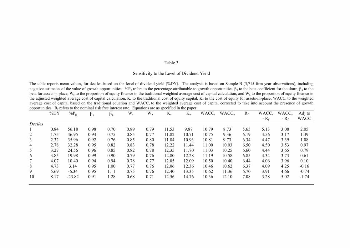
Table 3
Sensitivity to the Level of Dividend Yield The table reports mean values, for deciles based on the level of dividend yield (%DY). The analysis is based on Sample B (3,715 firm-year observations), including negative estimates of the value of growth opportunities. %Pg refers to the percentage attributable to growth opportunities, βs to the beta coefficient for the share, βa to the beta for assets in place, Ws to the proportion of equity finance in the traditional weighted average cost of capital calculation, and Wa to the proportion of equity finance in the adjusted weighted average cost of capital calculation, Ks to the traditional cost of equity capital, Ka to the cost of equity for assets-in-place, WACCs to the weighted average cost of capital based on the traditional equation and WACCa to the weighted average cost of capital corrected to take into account the presence of growth opportunities. Rf refers to the nominal risk free interest rate. Equations are as specified in the paper.
%DY %Pg βs βa Ws Wa Ks Ka WACCs WACCa Rf WACCs - Rf
WACCa - Rf
Adj to WACC
Deciles 1 0.84
56.18 0.98 0.70 0.89 0.79 11.53 9.87 10.79 8.73 5.65 5.13 3.08 2.052 1.75 46.95 0.94 0.75 0.85 0.77 11.82 10.71 10.75 9.36 6.19 4.56 3.17 1.393 2.32 35.96 0.92 0.76 0.85 0.80 11.84 10.93 10.81 9.73 6.34 4.47 3.39 1.084 2.78 32.28 0.95 0.82 0.83 0.78 12.22 11.44 11.00 10.03 6.50 4.50 3.53 0.975 3.27 24.56 0.96 0.85 0.82 0.78 12.35 11.70 11.03 10.25 6.60 4.44 3.65 0.796 3.85 19.98 0.99 0.90 0.79 0.76 12.80 12.28 11.19 10.58 6.85 4.34 3.73 0.617 4.07 10.40 0.94 0.94 0.78 0.77 12.05 12.09 10.50 10.40 6.44 4.06 3.96 0.108 4.73 3.14 0.95 1.00 0.77 0.76 12.06 12.36 10.46 10.62 6.37 4.09 4.25 -0.169 5.69 -6.34 0.95 1.11 0.75 0.76 12.40 13.35 10.62 11.36 6.70 3.91 4.66 -0.7410 8.17
-23.82 0.91 1.28 0.68 0.71 12.56 14.76 10.36 12.10 7.08 3.28 5.02 -1.74

0
5
10
15
20
25
30
35
40
45
50
1990 1992 1994 1996 1998 2000 2002 2004Sample Year
Sample A Sample B % Negative Pg
Fig. 1. Percentage Growth Opportunities
Notes: The figure shows the time-series variation in the estimated mean percentage of share prices accounted for by growth opportunities. Sample A refers to the sample of 2,571 firm-years with non-negative estimated values of growth opportunities (Pg), while Sample B refers to the full sample of 3,715 firm-years, including negative Pg. %Negative Pg shows the time-variation in the percentage proportion of the sample with negative estimated values for Pg. The estimations are based on an assumed equity risk premium of 6%, as in Table 2.

7
8
9
10
11
12
13
14
15
16
1990 1992 1994 1996 1998 2000 2002 2004Sample Year
WACCs WACCa
Fig. 2. Percentage Weighted Average Cost of Capital
Notes: The figure shows the time-series variation in the mean values of the weighted average cost of capital, estimated using the traditional (WACCs, as in equation 9) and the adjusted (WACCa, as in equation 10) model, as discussed in the text. The analysis is based on Sample A (2,571 cases).