Computing Multi-Species Chemical Equilibrium with an Algorithm Based on the

Reaction Extents

Juan Manuel Paz-Garcíaa,⇤, Björn Johannessona, Lisbeth M. Ottosena, Alexandra B. Ribeirob,José Miguel Rodríguez-Marotoc

aDepartment of civil Engineering, Technical University of Denmark, Brovej, Building 118, Dk 2800 Kgs. Lyngby, Denmark.bDepartment of Environmental Sciences and Engineering, Faculty of Sciences and Technology, New University of Lisbon, Caparica,

PortugalcDepartment of Chemical Engineering, Faculty of Sciences, University of Malaga, Campus de Teatinos, Malaga, Spain.

Abstract

A mathematical model for the solution of a set of chemical equilibrium equations in a multi-species and multiphasechemical system is described. The computer-aid solution of model is achieved by means of a Newton-Raphson methodenhanced with a line-search scheme, which deals with the non-negative constrains. The residual function, representingthe distance to the equilibrium, is defined from the chemical potential (or Gibbs energy) of the chemical system. Localminimums are potentially avoided by the prioritization of the aqueous reactions with respect to the heterogeneousreactions. The formation and release of gas bubbles is taken into account in the model, limiting the concentration ofvolatile aqueous species to a maximum value, given by the gas solubility constant.

The reaction extents are used as state variables for the numerical method. As a result, the accepted solution satisfiesthe charge and mass balance equations and the model is fully compatible with general reactive transport models.

Keywords: Chemical equilibrium, Speciation, Reaction extent, Reactive transport

1. Introduction

In a system at chemical equilibrium, the reactions takeplace at equal rates in their direct and reverse directionsand, therefore, the concentrations of the reacting substances(reactants and products) do not change with time. Thechemical equilibrium assumption (CEA) consists of consid-ering that all the species in the system have time enough toreach the equilibrium state. As a result, the time deriva-tive of the chemical equations becomes zero and a set ofalgebraic chemical concentration equations can be usedto mathematically describe such a system. Despite that,the equations describing multi-species chemical equilib-rium (MSCE) systems are strongly nonlinear and the ana-lytical solution cannot be found except for the most simplecases, being necessary the use of computer-aid approaches.

Numerical models based on the CEA may be used, forexample, to: (1) fit experimental data to chemical equi-librium state in a numerical speciation process, (2) to es-timate trace compounds concentrations based on the an-alytical measurements of species with significantly higherconcentrations, (3) to study the response of a chemical sys-tem in equilibrium with respect to external changes, (4)to study weathering mechanisms in geochemical systems,and (5) to model chemical interactions between the pore

⇤Corresponding authorEmail address: jugra@byg.dtu.dk (Juan Manuel Paz-García)

solution and the solid matrix in porous materials (Bethke,2008).

The reliability of the CEA depends on the time scale forthe speciation problem. A representative example wouldbe a reactive transport model under the local CEA inwhich the driving forces are chemical or electrical potentialgradients. In those cases, the transport rates of the maintransport mechanisms (diffusion, electromigration and elec-troosmosis) are slow enough to accept the equilibrium as-sumption except for those very slow heterogeneous reac-tions (Jacobs & Probstein, 1996; Morel & Hering, 1993).

Aqueous reversible reactions frequently have high ki-netic rates in both directions, towards the products andtowards the reactants, making the CEA acceptable in mostcases. Acids and bases dissociation or the seft-ionization ofwater, for example, can reach the equilibrium state in theorder of microseconds or even faster. Aqueous complexa-tion reactions are also usually quite fast, normally achiev-ing the equilibrium in the range from micro- to millisec-onds. In the case of heterogeneous reactions, such as ad-sorption/desorption, ion-exchange or precipitation/dissolutionreactions, their kinetic rates are commonly slower than theabove mentioned aqueous homogeneous reactions and theirrates may compete with the transport rates in some cases.

Some models for reactive transport through porous me-dia taking into consideration the kinetics of the chemicalsystem have been presented, as e.g. (Johannesson, 2009;Lichtner, 1985; Steefel & Van Cappellen, 1990). Neverthe-

Preprint submitted to Computers And Chemical Engineering April 4, 2013

Nomenclature

List of symbolsa chemical activity (�)a chemical activities vector (�)A Davies constant (kg mol�1)1/2

b Setschenow constantf residual functionf residual function vector�G Gibbs energy�h numerical incrementI Ionic strengthJ jacobian matrixK equilibrium constantKH Henry’s constantk equilibrium constant matrixm molal concentration

�mol kg�1

�

M number of reactions (�)M stoichiometric matrix (�)n molal amount (mol)n molal amounts vector (mol)N number of species (�)P pressure (atm)R universal gas constant

�J K�1 mol�1

�

T absolute temperature (K)x reaction extent (mol)x reaction extents vector (mol)z ionic charge (�)Greek letters� activity factor (�)� line-search scaling factor (�)µ chemical potential

�J mol�1

�

⌫ stoichiometric coefficient (�)Subscriptseq equilibriumi chemical speciesinit initialmax maximalmin minimalr equilibrium reaction

less, models under the chemical equilibrium assumptionare more extensively used, as e.g. (Al-Hamdan & Reddy,2008; Javadi & Al-Najjar, 2007; Rubin, 1983; Vereda-Alonsoet al., 2007). Rate-controlled equilibrium models, whichare considered more realistic, include a set of feasible re-actions capable to reach the equilibrium in the time scale ofthe transport process and a parallel solution of the kineticequations for the slow and/or the irreversible reactions(Koukkari & Pajarre, 2006; Ribeiro et al., 2005; Steyeret al., 2005).

The most accepted mathematical algorithm for MSCEcalculation is based on the Morel’s Tableau stoichiometricmethod (Morel & Hering, 1993; Morel & Morgan, 1972),which basically consists in dividing the set of chemicalspecies in a number of master species (or components) andsecondary species (or compounds). Secondary species are

defined as a combination of master species by means ofstoichiometric chemical equilibrium equations. In (Reed,1982) and (Bethke, 2008), comprehensive compilations ofdifferent proposed models for the mathematical solution ofchemical equilibrium problems can be found. This litera-ture review will not be repeated here.

Several computer programs for MSCE have been re-leased. Some of the most used are PHREEQC (Parkhurst& Appelo, 1999), PHREEQCi (Charlton et al., 1997), WA-TEQ4F (Ball & Nordstrom, 1991), MINTEQ (Petersonet al., 1987), EQ3/6 (Wolery, 1992) and GEMS (Remy,2004). Coupling these kind of stand-alone programs withmore general codes for different purposes is possible. Nev-ertheless, exporting and importing data between differ-ent programs normally involves the participation of theprogram user, as well as significant computational time,making simulations slow or, sometimes, unfeasible. Conse-quently, the implementation of tailor-made codes is almostalways necessary for more complex problems (Rodriguez-Maroto & Vereda-Alonso, 2009).

In summary, numerical strategies for computing chemi-cal equilibrium problems are classified into two main groups:stoichiometric and non-stoichiometric algorithms (van Baten& Szczepanski, 2011; Blomberg & Koukkari, 2011; Bras-sard & Bodurtha, 2000; Carrayrou et al., 2002). Stoichio-metric algorithms converge on the solution of a set of si-multaneous mass balance and mass action equations ateach iteration, while non-stoichiometric algorithms aim adirect minimization of the Gibbs energy functions of thechemical species constrained by mass balances.

The most popular stoichiometric algorithm uses theconcentration of the master species as the independentstate variable while the residual function to be minimizedin the numerical procedure is defined from the mass bal-ance on the chosen master species and the saturation in-dex of the existing solid components. The mass balanceof protons is replaced by the charge balance equation, inthis approach, for two reasons: (1) to avoid consideringthe water as a chemical species in the setup, and (2) toassure charge neutrality in the equilibrated solution. Thismethod has shown accurate results and has been the basefor some of the chemical equilibrium models listed above.

In this work, we propose a stoichiometric method forMSCE, based on the Tableau’s concept, iterating on thereaction extents and submitted to the non-negative com-position constraints. Despite this method shows a highertendency of falling into the so-called local minima, someadvantages may be remarked: (1) A model based on thereaction extent is compatible with rate-controlled mod-els dealing simultaneously with chemical equilibrium andchemical kinetics, and (2) for a given value of the reactionextent, the mass and the charge conservation principles arealways satisfied increasing the compatibility with generalreactive-transport models.

A Newton-Raphson (NR) method, enhanced with aline-search (LS) with backtracking scheme, is used for thesolution of the nonlinear system of equations (Press et al.,

1992; Wolery & Walters, 1975). The model includes het-erogeneous precipitation/dissolution reactions, as well asthe possibility of the release of bubbles of volatile aqueousspecies to the surrounding atmosphere. Logarithm scale isused in order to (1) convert the exponential mass actionequation into algebraical equations, (2) assure the non-negative constrain, and (3) to minimize the error inducedby the programing language when using values with signif-icant differences in their orders of magnitude, as commonin multi-species chemical systems.

2. Mathematical model

2.1. Stoichiometry of the chemical system

The analytical description of the chemical equilibriumproblem is carried out by a set of nonlinear algebraic equa-tions formulated from the mass balance and the actionmass equations describing the chemical system (Bethke,2008; Rawlings & Ekerdt, 2002; Stumm & Morgan, 1970).

The total number of species, N , is divided into the M

secondary species and the (N � M) master species thatdefine them. The chosen master species must represent allthe chemical elements in the system (Rodriguez-Maroto &Vereda-Alonso, 2009).

For a set of N chemical species, the M stoichiometricequations are defined as:

NX

i=1

⌫

r,i

n

i

= 0 , r = 1, 2, ..., M (1)

where n

i

(mol) denotes the total amount of the i

th chem-ical species in the system and ⌫

r,i

is the stoichiometriccoefficient for the i

th species in the r

th reaction. Herein,the stoichiometric equations are written in the form of dis-sociation or dissolution reactions, being the stoichiometriccoefficients of the reactants defined with negative values.By definition, each secondary species participate only inthe r

th stoichiometric equation that describes it.In the following, we will use the chemical system re-

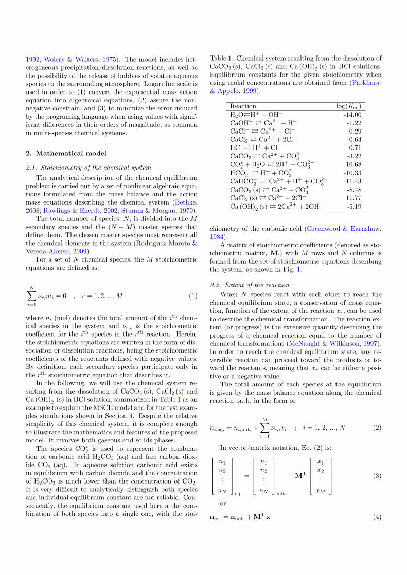
sulting from the dissolution of CaCO3 (s), CaCl2 (s) andCa (OH)2 (s) in HCl solution, summarized in Table 1 as anexample to explain the MSCE model and for the test exam-ples simulations shown in Section 4. Despite the relativesimplicity of this chemical system, it is complete enoughto illustrate the mathematics and features of the proposedmodel. It involves both gaseous and solids phases.

The species CO⇤2 is used to represent the combina-

tion of carbonic acid H2CO3 (aq) and free carbon diox-ide CO2 (aq). In aqueous solution carbonic acid existsin equilibrium with carbon dioxide and the concentrationof H2CO3 is much lower than the concentration of CO2.It is very difficult to analytically distinguish both speciesand individual equilibrium constant are not reliable. Con-sequently, the equilibrium constant used here a the com-bination of both species into a single one, with the stoi-

Table 1: Chemical system resulting from the dissolution ofCaCO3 (s), CaCl2 (s) and Ca (OH)2 (s) in HCl solutions.Equilibrium constants for the given stoichiometry whenusing molal concentrations are obtained from (Parkhurst& Appelo, 1999).

Reaction log(Keq)H2O�H+ + OH� -14.00CaOH+ � Ca2+ + H+ -1.22CaCl+ � Ca2+ + Cl� 0.29CaCl2 � Ca2+ + 2Cl� 0.64HCl � H+ + Cl� 0.71CaCO3 � Ca2+ + CO2�

3 -3.22CO⇤

2 + H2O � 2H+ + CO2�3 -16.68

HCO�3 � H+ + CO2�

3 -10.33CaHCO+

3 � Ca2+ + H+ + CO2�3 -11.43

CaCO3 (s) � Ca2+ + CO2�3 -8.48

CaCl2 (s) � Ca2+ + 2Cl� 11.77Ca (OH)2 (s) � 2Ca2+ + 2OH� -5.19

chiometry of the carbonic acid (Greenwood & Earnshaw,1984).

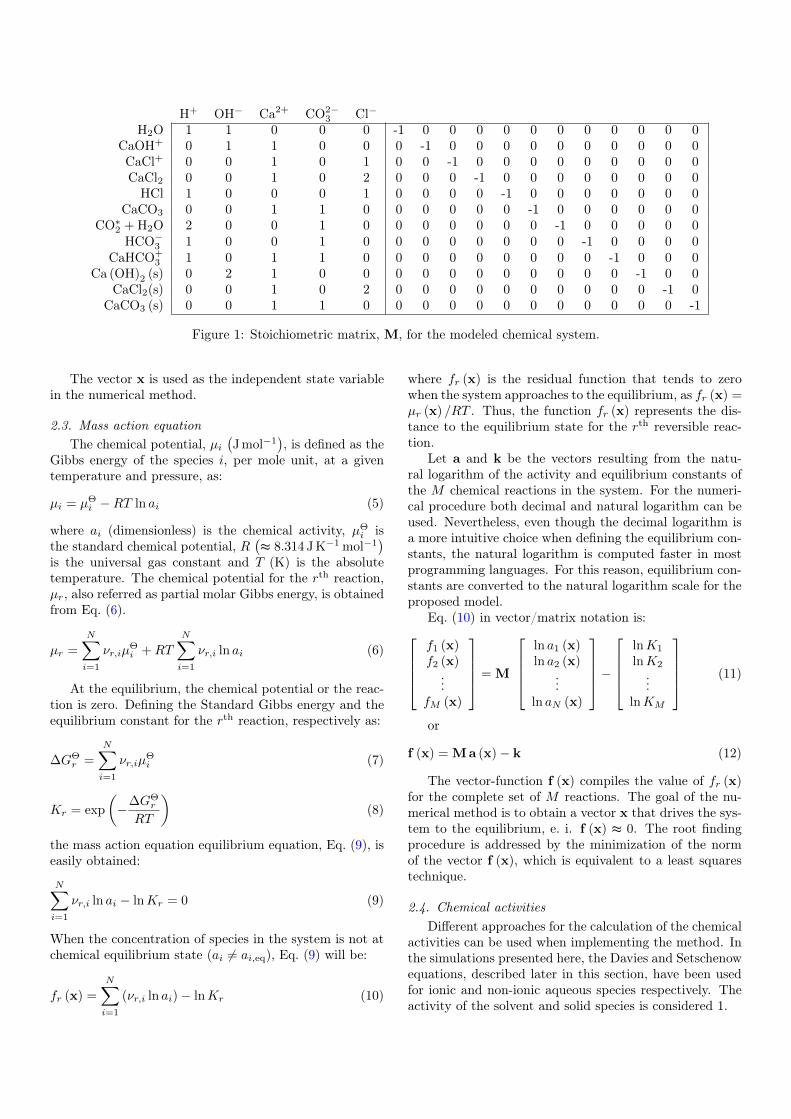
A matrix of stoichiometric coefficients (denoted as sto-ichiometric matrix, M,) with M rows and N columns isformed from the set of stoichiometric equations describingthe system, as shown in Fig. 1.

2.2. Extent of the reaction

When N species react with each other to reach thechemical equilibrium state, a conservation of mass equa-tion, function of the extent of the reaction x

r

, can be usedto describe the chemical transformation. The reaction ex-tent (or progress) is the extensive quantity describing theprogress of a chemical reaction equal to the number ofchemical transformations (McNaught & Wilkinson, 1997).In order to reach the chemical equilibrium state, any re-versible reaction can proceed toward the products or to-ward the reactants, meaning that x

r

can be either a posi-tive or a negative value.

The total amount of each species at the equilibriumis given by the mass balance equation along the chemicalreaction path, in the form of:

n

i,eq.

= n

i,init. +MX

r=1

⌫

r,i

x

r

; i = 1, 2, ..., N (2)

In vector/matrix notation, Eq. (2) is:2

6664

n1

n2...

n

N

3

7775

eq.

=

2

6664

n1

n2...

n

N

3

7775

init.

+ MT

2

6664

x1

x2...

x

M

3

7775(3)

or

neq.

= ninit. + MT x (4)

H+ OH� Ca2+ CO2�3 Cl�

H2O 1 1 0 0 0 -1 0 0 0 0 0 0 0 0 0 0 0CaOH+ 0 1 1 0 0 0 -1 0 0 0 0 0 0 0 0 0 0CaCl+ 0 0 1 0 1 0 0 -1 0 0 0 0 0 0 0 0 0CaCl2 0 0 1 0 2 0 0 0 -1 0 0 0 0 0 0 0 0

HCl 1 0 0 0 1 0 0 0 0 -1 0 0 0 0 0 0 0CaCO3 0 0 1 1 0 0 0 0 0 0 -1 0 0 0 0 0 0

CO⇤2 + H2O 2 0 0 1 0 0 0 0 0 0 0 -1 0 0 0 0 0

HCO�3 1 0 0 1 0 0 0 0 0 0 0 0 -1 0 0 0 0

CaHCO+3 1 0 1 1 0 0 0 0 0 0 0 0 0 -1 0 0 0

Ca (OH)2 (s) 0 2 1 0 0 0 0 0 0 0 0 0 0 0 -1 0 0CaCl2(s) 0 0 1 0 2 0 0 0 0 0 0 0 0 0 0 -1 0

CaCO3 (s) 0 0 1 1 0 0 0 0 0 0 0 0 0 0 0 0 -1

Figure 1: Stoichiometric matrix, M, for the modeled chemical system.

The vector x is used as the independent state variablein the numerical method.

2.3. Mass action equation

The chemical potential, µ

i

�J mol�1

�, is defined as the

Gibbs energy of the species i, per mole unit, at a giventemperature and pressure, as:

µ

i

= µ

⇥i

� RT ln a

i

(5)

where a

i

(dimensionless) is the chemical activity, µ

⇥i

isthe standard chemical potential, R

�t 8.314 J K�1 mol�1

�

is the universal gas constant and T (K) is the absolutetemperature. The chemical potential for the r

th reaction,µ

r

, also referred as partial molar Gibbs energy, is obtainedfrom Eq. (6).

µ

r

=NX

i=1

⌫

r,i

µ

⇥i

+ RT

NX

i=1

⌫

r,i

ln a

i

(6)

At the equilibrium, the chemical potential or the reac-tion is zero. Defining the Standard Gibbs energy and theequilibrium constant for the r

th reaction, respectively as:

�G

⇥r

=NX

i=1

⌫

r,i

µ

⇥i

(7)

K

r

= exp

✓��G

⇥r

RT

◆(8)

the mass action equation equilibrium equation, Eq. (9), iseasily obtained:

NX

i=1

⌫

r,i

ln a

i

� ln K

r

= 0 (9)

When the concentration of species in the system is not atchemical equilibrium state (a

i

6= a

i,eq), Eq. (9) will be:

f

r

(x) =NX

i=1

(⌫r,i

ln a

i

) � ln K

r

(10)

where f

r

(x) is the residual function that tends to zerowhen the system approaches to the equilibrium, as f

r

(x) =µ

r

(x) /RT . Thus, the function f

r

(x) represents the dis-tance to the equilibrium state for the r

th reversible reac-tion.

Let a and k be the vectors resulting from the natu-ral logarithm of the activity and equilibrium constants ofthe M chemical reactions in the system. For the numeri-cal procedure both decimal and natural logarithm can beused. Nevertheless, even though the decimal logarithm isa more intuitive choice when defining the equilibrium con-stants, the natural logarithm is computed faster in mostprogramming languages. For this reason, equilibrium con-stants are converted to the natural logarithm scale for theproposed model.

Eq. (10) in vector/matrix notation is:2

6664

f1 (x)f2 (x)

...f

M

(x)

3

7775= M

2

6664

ln a1 (x)ln a2 (x)

...ln a

N

(x)

3

7775�

2

6664

ln K1

ln K2...

ln K

M

3

7775(11)

or

f (x) = Ma (x) � k (12)

The vector-function f (x) compiles the value of f

r

(x)for the complete set of M reactions. The goal of the nu-merical method is to obtain a vector x that drives the sys-tem to the equilibrium, e. i. f (x) t 0. The root findingprocedure is addressed by the minimization of the normof the vector f (x), which is equivalent to a least squarestechnique.

2.4. Chemical activities

Different approaches for the calculation of the chemicalactivities can be used when implementing the method. Inthe simulations presented here, the Davies and Setschenowequations, described later in this section, have been usedfor ionic and non-ionic aqueous species respectively. Theactivity of the solvent and solid species is considered 1.

In the present model, the activity values of each aque-ous chemical species are obtained from the amount n

i

(x)calculated in each numerical iteration step. The activity isdefined from the molal concentration m

i

�mol kg�1

�, the

activity factor �

i

(dimensionless), and the standard con-centration m

⇥i

�mol kg�1

�necessary to ensure that the

activity is also dimensionless.

a

i

= �

i

m

i

m

⇥i

(13)

The Davies equation, Eq. (14), is an empirical exten-sion of the Debye-Hückel equation. The Davies equationis considered to be a reasonable approximation even atrelatively high ionic concentrations.

ln �

i

= Az

2i

pI

1 +p

I

� 0.3I

!(14)

where A = �1.172 (kg mol�1)1/2, z

i

�mol mol�1� is the

ionic charge and I

�mol kg�1

�is the ionic strength of the

electrolyte media, calculate by:

I =1

2

NX

i=1

m

i

z

2i

(15)

For the case of non-ionic aqueous species, the activityfactor is obtained using the Setschenow relation, as

ln �

i

= b

i

I (16)

where b

i

is the Setschenow coefficient. In the simulationspresented in this work, b

i

= 0.1 is used for all non-chargedaqueous species, as done in (Parkhurst & Appelo, 1999).

The validity of the Davies and Setschenow equations islimited to values of ionic strength equal to or lower than0.5. Over this limit, spurious results may be obtained.Some alternative theories, such as the Specific Ion Inter-action Theory (SIT) (Guggenheim & Turgeon, 1955) andthe Pitzer activity coefficients (Pitzer, 1973) could be usedto increase the range of validity of the activity coefficients.

2.5. Precipitation/dissolution heterogeneous equilibrium

Heterogeneous precipitation and dissolution reactionshave some key differences with respect to the aqueous com-plexation. First, the activity of the solids is set to theunity value. Consequently, in the mass action equationfor precipitation/dissolution reactions, the excess of solidsin saturated solutions does not affect the concentration ofaqueous species.

The existence of solid species is limited by the so-called saturation index (SI), which determines if the elec-trolyte solution is saturated or undersaturated with re-spect to the solid defined by a precipitation/dissolutionreaction. Indeed, the equilibrium constant for a precipita-tion/dissolution reaction is typically denoted as solubility

product. The value of the residual function f

r

(x) is usedas an indicator of the saturation index, in the form:(

f

r

(x) < 0 undersaturated

f

r

(x) � 0 saturated(17)

If a solution is undersaturated, the corresponding solidwould be completely dissolved and it will not participatein the equilibrium process. Therefore, its contribution inthe residual function must be ignored. The numerical pro-cedure, for any iteration, consists of:

1. Identify the precipitation/dissolution reactions thatare undersaturated, i.e. f

r

(x) < 02. Force the reaction extent for undersaturated reac-

tions to be the maximum (complete dissolution).3. Ignore the contribution of f

r

(x) < 0 to the calcula-tion of the norm of the residual.

In conditions close to the equilibrium state, the propertyf

r

(x) can oscillate around the value of zero, and so the re-action can oscillate around the saturated/undersaturatedstatus during the speciation process. Consequently, thisstrategy has to be followed iteration-by-iteration.

Furthermore, using the density and the molecular mass,the volume fraction occupied by the solution and the solidscan be measured. As a result, the porosity of the porousmedia can be calculated, which is a crucial parameterin the case of reactive-transport modeling through theseporous media.

2.6. Vapor-liquid heterogeneous reactions

Vapor-liquid heterogeneous reactions are difficult tocouple with the previously described aqueous complexa-tion and mineral dissolution reactions, because many ex-tra assumptions are necessary. If the time scale is largeenough to assume the equilibrium condition for the vapor-liquid equilibrium, and in the case of very dilute systems,the Henry’s law may be used. Henry’s law states that, at aconstant temperature, the amount of a given gas dissolvedin a volume of liquid is directly proportional to the par-tial pressure of that gas in equilibrium with that liquid, bymeans of the so-called Henry�s constant.

Pi(g) = KH mi(aq) (18)

This kind of approach is used to calculate the concen-tration of gaseous species in equilibrium with the liquidsystem in many geochemical speciation models, as e.g. in(Parkhurst & Appelo, 1999).

For the case of chemical equilibrium models designedto be coupled with reactive-transport in porous media,some extra considerations have to be taken. For exam-ple, depending on the time scale of the speciation prob-lem, assuming vapor-liquid equilibrium between the at-mospheric species and the aqueous species can lead tounrealistic results. This is the case of the carbonic acidequilibrium. If we consider a porous material in contact

with the atmosphere, being the atmospheric partial pres-sure of the carbon dioxide a constant value, the concen-tration of the species CO2(aq), HCO�

3 , CO�23 among oth-

ers, would be fixed. Consequently, the system would bestrongly buffered by the carbonic acid equilibrium. Rateconstants for the reversible reaction between the gaseousand aqueous CO2 equilibrium is slow with respect to theaqueous complexation reactions. Thus, the buffered capac-ity of the atmospheric CO2 in the porous system would beoverestimated if the equilibrium assumption is accepted.

According to this, a different approach is taken in thismodel. First, the system is assumed to be at constant pres-sure (normally 1 atm). The Henry’s constant is used todefine the maximum amount of the volatile species aque-ous concentration that would produce the release of gasbubbles from the system. For example, the concentrationof gaseous carbonic acid would be given by:

PCO2(g) = KH mCO2(aq) (19)

Mathematically, this assumption is equivalent to con-sider a maximum limit value for the aqueous concentrationof volatile compounds. For the case of CO2 (g) at roomtemperature and PCO2 = Ptotal = 1 (atm), the maximumCO2 (aq) concentration would be given by:

mCO2(aq)

��max

=1

KH= 3.36 ⇥ 10�2

�mol kg�1

�(20)

3. Numerical implementation

3.1. Newton-Raphson method for non-linear systems

The value of the reaction extents vector x that assuresglobal equilibrium is obtained by an iterative procedurebased on a NR method with a line-search technique tosatisfy the non-negative restriction (Press et al., 1992).The numerical procedure is summarized in the pseudo-code shown in Fig. (2).

The NR method for a non-linear matrix system of equa-tions indicates the next iteration value for the unknowns,xnew, obtained from the present value, xold, by adoptinga numerical increment, �x, toward the direction that de-creases the global residual function.

xnew = xold + �x (21)

The Taylor’s series expansion of the residual functionf(x) is used.

f (xnew) = f (xold) + J �x + O (�x)2 (22)

where O(�x)2 represents the error related to terms withorder greater than 2 and J is the Jacobian matrix of partialderivatives defined as:

J =⇥

@f@x1

· · · @f@xM

⇤=

2

64

@f1

@x1· · · @f1

@xM

.... . .

...@fM

@x1· · · @fM

@xM

3

75 (23)

Ignore the solids during

the next iteration!

Refine numerical !Parameters!

Line search step!

Newton-Raphson step!

Compute J !

START!

END!

YES!

NO!

YES!

NO!

NO!

YES!

Compute f!

Compute!

Compute !

kf (xnew)k < kf (xold)k ?

f (xnew) = Ma (xnew) � k

n (xnew)

k < kmax ?

a (xnew)

xnew = xold + ��x

kf (xnew)k < kf (x)kmin ?

any n

i

< 0 ?

xold = xnew

kf (xold)k = kf (xnew)k

�x = �J�1f (xold)

,!� = 1

YES!

NO!

Line search with!backtracking!

Convergence! strategies !

Last time = NO?!YES!NO!

�new =�old

�

⇤

k = 1

NO!

YES!

k = k + 1

j = j + 1j < jmax?

j = 1

�hnew =�hold

h

⇤

Figure 2: Flowchart for the NR method

The next step in the NR method adopted will be givenfrom the fact that the target is to obtain f (xnew) = 0.Ignoring the term O(�x)2, the increment in the extent ofall considered reactions is, therefore, obtained as:

�x = �J�1f (xold) (24)

3.2. Line-search with backtracking enhancement

A line-search with backtracking enhancement is usedin the NR method. Line-search iterative methods usuallyrequire an important computational effort due to a largenumber of iterations until convergence. As mentioned be-fore the vector �x indicates the direction in which theresidual decreases but it carries no information about themagnitude of the increment in the extent of the reactions.

If the step is to long, the system may get far from the equi-librium, failing in minimizing the residual. In addition tothis, the system is restricted to the non-negative physicalconstrain for the concentrations or amounts of all chemicalspecies (van Baten & Szczepanski, 2011).

In the LS method, a scalar factor � is used to con-trol the magnitude of the increment calculated by the NRmethod. Eq. (25) is used instead of Eq. (21).

xnew = xold + ��x (25)

The optimal � value is obtained by a try-and-error al-gorithm, following a decreasing sequence given by the ge-ometric progression according to Eq. (26), with an initialvalue of �init = 1.

�new = �old/�

⇤ (26)

3.3. Numerical computation of the Jacobian

Due to the strong non-linearity of the system of equa-tions, the analytical calculation of the Jacobian matrixis unfeasible. Therefore, an incomplete Newton-Raphsonscheme is used, based on a numerical computation of theJacobian matrix, achieved by central differences vector dif-ferentiation, as:

@f (x)

@x

r

=f (x + �x

r

) � f (x � �x

r

)

2�x

r

(27)

The increment �x

r

used in the calculation of the Jaco-bian plays an important role in the convergence capabilityof the problem. The reaction extent of the different equi-librium equations may differ significantly, and therefore aconstant �x

r

would find unwanted local minimums ruin-ing the iterative approach. In order to avoid this problem,the value �x

r

used is scaled to the value of the vector xduring any iteration:

�x

r

= |xr

| �h (28)

where �h is a value between �hinit and �hmin.Incomplete Newton-Raphson schemes have linear con-

vergence rates, while analytical calculated Jacobian wouldconverge quadratically. In addition to this, the numericalcalculation of the Jacobian matrix usually requires a sig-nificant amount of computational time. In Algorithm (1)we propose a vectorized implementation for computing thenumerical Jacobian. In this context, vectorized implemen-tation means that no loops are used for the calculationof the Jacobian, using only matrix algebra operations.Therefore, instead of using a loop for the calculation ofthe M vectors resulting from the solution of Eq. (27) forthe M derivatives, the problem is solved using a singlematrix operation. Eq. (4) in matrix notation would be:

⇥n1 · · · n

M

⇤eq.

=⇥

n1 · · · nM

⇤init.

+

+ MT⇥

x1 · · · xM

⇤

or

Neq.

= Ninit. + MT X (29)

As the Jacobian matrix is computed several times dur-ing the process, using the proposed vectorized algorithm,the entire method is between 10 to 100 times faster thancompared to using computational “for” or “while” loops.

3.4. Convergence strategies

The main disadvantage of using the reaction extent asthe state variable is that there is a moderate to high riskof falling into a local (relative) minimum, as illustrated inFig 3. The probability of finding local minimums dependson the distance to the equilibrium from the initial set ofconcentrations. A good initial estimation of the state vari-able x is needed (Brassard & Bodurtha, 2000).

In dynamic problems, such as reactive transport pro-cesses, if small enough time increments are used, the dis-tance to the equilibrium is small and an initial estimationof x = 0 is usually valid. When using the model for thespeciation of compounds in trace concentration, an initialguess can be estimated based on the concentration of themajor species. If there is no information about the equi-librium concentrations at the beginning of the calculation,an initial guess is suggested based on the vector k, withthe equilibrium constants at logarithm scale, which wouldindicate the tendency of the species toward the dissolutionor the dissociation.

Even when using a good initial guess, it may happenthat the NR with LS method fails at finding the equilib-rium in some specific cases. In order to reduce the risk offinding local minima, some extra considerations have beentaken. In this context, the “convergence strategies” blockshown in Fig. 2, includes two different procedures, whichare alternatively used when the LS method reaches themaximum value of iterations without reducing the resid-ual function.

1. Refine numerical parameters

Figure 3: Chemical equilibrium as a function of the reac-tion extent

Algorithm 1 Pseudo-code for the numerical calculationof the Jacobian matrix

1. Create a matrix X+�X (size M by M) includingthe current value of the state variable x summed toa diagonal matrix with the finite increment for thenumerical calculation of the derivatives:

X+�X = X+diag(�X)

where

X+�X =

2

64(x1 + �x1) · · · x1

.... . .

...x

M

· · · (xM

+ �x

M

)

3

75

2. Compute a matrix N with the molar amount ofspecies, as a function of X+�X:

Neq.

= Ninit. + MT X+�X

3. Compute the matrix A formed from the activities,using the matrix N

eq.

and the same agreements forthe activity factors.

4. Using K =⇥

k · · · k⇤, compute the residual ma-

trix function, F�X+�X

�as:

F�X+�X

�= MA � K

5. Repeat steps 1-4 using X��X = X�diag(�X)6. Compute the Jacobian matrix as:

J =F�X+�X

�� F

�X��X

�

2�X

where the latter operation is done “term-by-term”instead of by standard matrix division, using the fullmatrix of increments in the form:

�X =

2

64�x1 · · · �x

M

.... . .

...�x1 · · · �x

M

3

75

If the norm of the residual function is not minimizedfor a certain number of iterations kmax, the incre-mental parameter for the numerical calculation ofthe Jacobian is reduced ten times, i.e. �hnew =�hold/h

⇤. If the value �hmin is reached and, eventhough, the residual kf (x)k is not reduced, the localminimum is accepted as a valid result.

2. Ignore precipitation/dissolution reactions

The second procedure consists of ignoring the pre-cipitation/dissolution reactions during one iteration.This innovative method is based on the concept that,even when the equilibrium assumption is accepted,the kinetic of the heterogeneous reactions is almostalways lower than the homogeneous aqueous reac-tions.

As an example of this kind of behavior, Eq. (30) shows thedissolution reaction of kaolinite as a function of the mas-ter species H+, H2O, H4SiO4 and Al3+. According to thisstoichiometry and the Le Châtelier’s principle, an exter-nal increment in the pH in the system containing kaoliniteshould produce the precipitation of the mineral, what ischaracterized with a release of protons which will coun-teract the pH change. On the other hand, the pH alsoaffects to the species H4SiO4 and Al3+. H4SiO4 is an acidand can dissociate releasing protons, and Al3+ reacts withhydroxides to form different aluminum hydroxides. Con-sequently, the kaolin is forced to precipitate, due to thepH increase, but it is also forced to dissolve in order tocounteract the consumption of H4SiO4 and Al3+, due tothe same pH change. This kind of situations can, in someinstances, lead to the development of a local minimum.

Al2Si2O5 (OH)4 + 6H+ � H2O + 2H4SiO4 + 2Al3+ (30)

If one takes into account the kinetic rates of the re-action, it can be assured that the aqueous complexationreactions of H4SiO4 and Al3+ are faster than the precipi-tation/dissolution reaction. So, these two aqueous specieswould react first in order to counteract the pH changesand so the kaolinite would be forced to the dissolution.This is congruent with the experimental results observedin (Carroll & Walther, 1990).

4. Test examples

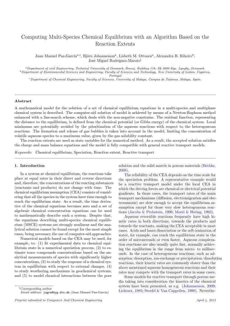
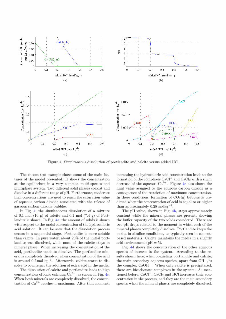
A test example is shown based on the chemical systemdescribed in Table 1. In this test example, the concen-tration in equilibrium of calcite, CaCO3, and portlandite,Ca(OH)2, in 1 kg of HCl solution at different concentra-tions is computed. For the simulations, the minerals areassumed in equilibrium with 1 kg of pure water. HCl isprogressively added to the solution, to cover a range from0 until 0.6 mol per kg of water. The equilibrium concentra-tion of aqueous species, the amount of precipitated solidsand the pH are shown with respect to the amount of acidadded to the system.

(a) (b)

(c) (d)

Figure 4: Simultaneous dissolution of portlandite and calcite versus added HCl

The chosen test example shows some of the main fea-tures of the model presented. It shows the concentrationat the equilibrium in a very common multi-species andmultiphase system. Two different solid phases coexist anddissolve in a different range of pH. Furthermore, moderatehigh concentrations are used to reach the saturation valueof aqueous carbon dioxide associated with the release ofgaseous carbon dioxide bubbles.

In Fig. 4, the simultaneous dissolution of a mixtureof 0.1 mol (10 g) of calcite and 0.1 mol (7.4 g) of Port-landite is shown. In Fig. 4a, the amount of solids is shownwith respect to the molal concentration of the hydrochloricacid solution. It can be seen that the dissolution processoccurs in a sequential stage. Portlandite is more solublethan calcite. In pure water, about 20% of the initial port-landite was dissolved, while most of the calcite stays inmineral phase. When increasing the concentration of theacid, portlandite tends to dissolve. The portlandite min-eral is completely dissolved when concentration of the acidis around 0.2 mol kg�1. Afterwards, calcite starts to dis-solve to counteract the addition of extra acid in the media.

The dissolution of calcite and portlandite leads to highconcentrations of ionic calcium, Ca2+, as shown in Fig. 4c.When both minerals are completely dissolved, the concen-tration of Ca2+ reaches a maximum. After that moment,

increasing the hydrochloric acid concentration leads to theformation of the complexes CaCl+ and CaCl2 with a slightdecrease of the aqueous Ca2+. Figure 4c also shows thelimit value assigned to the aqueous carbon dioxide as aconsequence of the restriction of maximum concentration.In these conditions, formation of CO2(g) bubbles is pre-dicted when the concentration of acid is equal to or higherthan approximately 0.28 mol kg�1.

The pH value, shown in Fig. 4b, stays approximatelyconstant while the mineral phases are present, showingthe buffer capacity of the two solids considered. There aretwo pH drops related to the moment in which each of themineral phases completely dissolves. Portlandite keeps themedia in alkaline conditions, as typically seen in cement-based materials. Calcite maintains the media in a slightlyacid environment (pH = 5).

Fig. 4d shows the concentration of the other aqueousspecies of interest in the system. According to the re-sults shown here, when coexisting portlandite and calcite,the main secondary aqueous species, apart from OH�, isthe complex CaOH+. When only calcite is precipitated,there are bicarbonate complexes in the system. As men-tioned before, CaCl+, CaCl2 and HCl increases their con-centration in the process, and they are the main secondaryspecies when the mineral phases are completely dissolved.

Table 2: Numerical parameters used in the test simulations

Parameter value�

⇤ 2�hinit. 2�25

�hmin 2�250

h

⇤ 225

kmax 10jmax 250kf (x)kmin 10�10

Table 2 collects the numerical parameters used in thesimulations presented here. A total of 500 simulations weredone to meet the entire range of HCl concentrations. Foran algorithm implemented in Matlab® 2012, and run ina 2.3 GHz Intel Core i5 computer with 4 GB 1333 MHzDDR3, the computing time was 107.13 s.

Conclusions

A method for computing chemical equilibrium specia-tion problems has been described, based on the extent ofeach chemical reaction of the system. The numerical solu-tion method is based on a quasi-NR method in which theJacobian matrix is formed by a numerical technique ratherthan being calculated analytically. In this context, a vec-torized implementation of the Jacobian matrix is proposedin order to significantly reduce the computational time. Aline search approach is used to deal with the non-negativeconcentrations constraint of all the chemical species.

The presented algorithm is designed to work in a multi-species and multiphase chemical systems under the as-sumption of chemical equilibrium. Problems associatedwith local minimums are potentially avoided by the prior-itization of the aqueous reactions with respect to the soliddissolution or precipitation reactions. This prioritizationmethod is based on the assumption that that the kineticrates of reactions involving only aqueous species are fasterthan those involving solid mineral phases.

The formation of gaseous species is included in themodel by allowing free release of gas bubbles of gaseousspecies when those bubbles have a higher pressure thanthe surrounding liquid media and vapor phase. This fea-ture limits the concentration of volatile aqueous species toa maximum value given by the gas solubility constant.

A test example has been used to illustrate the mainfeatures of the model presented here. The use of the extentof the reactions as the state variable makes the presentedalgorithm suitable for more general problems, in which athorough control of the electrical balance is required.

Acknowledgments

Authors acknowledge The Danish Agency of ScienceTechnology and Innovation. This research was funded aspart of the project “Fundamentals of Electrokinetics in

In-homogeneous Matrices”, with project number 274-08-0386. J.M. Rodríguez-Maroto acknowledges the financialsupport from the Ministerio de Ciencia e Innovación ofthe Spanish Government through the project ERHMES,CTM2010-16824, and FEDER funds.

—————–

References

Al-Hamdan, A. Z., & Reddy, K. R. (2008). Electrokinetic reme-diation modeling incorporating geochemical effects. J. Geotech.Geoenviron., 134 , 91–105.

Ball, J. W., & Nordstrom, D. K. (1991). User’s manual for WA-TEQ4F, with revised thermodynamic data base and test cases forcalculating speciation of major, trace, and redox elements in nat-ural waters. US Geological Survey Denver, CO.

van Baten, J., & Szczepanski, R. (2011). A thermodynamic equi-librium reactor model as a cape-open unit operation. Computersand Chemical Engineering, 35 , 1251–1256.

Bethke, C. M. (2008). Geochemical and biogeochemical reaction mod-eling. (2nd ed.). New York: Cambridge University Press.

Blomberg, P. B. A., & Koukkari, P. S. (2011). A systematic methodto create reaction constraints for stoichiometric matrices. Com-puters and Chemical Engineering, 35 , 1238–1250.

Brassard, P., & Bodurtha, P. (2000). A feasible set for chemicalspeciation problems. Comput. Geosci., 26 , 277–291.

Carrayrou, J., Mose, R., & Behra, P. (2002). New efficient algorithmfor solving thermodynamic chemistry. AIChE J., 48 , 894–904.

Carroll, S., & Walther, J. (1990). Kaolinite dissolution at 25, 60,and 80 c. Am. J. Sci , 290 , 797–810.

Charlton, S. R., Macklin, C. L., & Parkhurst, D. L. (1997).Phreeqci—a graphical user interface for the geochemical com-puter program phreeqc. Water Resources Investigation Report ,97 , 4222.

Greenwood, N. N., & Earnshaw (1984). Chemistry of the Elements.Pergamon press Oxford etc.

Guggenheim, E., & Turgeon, J. (1955). Specific interaction of ions.Trans. Faraday Soc., 51 , 747–761.

Jacobs, R. A., & Probstein, R. F. (1996). Two-dimensional modelingof electroremediation. AIChE J., 42 , 1685–1696.

Javadi, A., & Al-Najjar, M. (2007). Finite element modeling of con-taminant transport in soils including the effect of chemical reac-tions. J. Hazard. Mater., 143 , 690–701.

Johannesson, B. (2009). Ionic diffusion and kinetic homogeneouschemical reactions in the pore solution of porous materials withmoisture transport. Comput. Geotech., 36 , 577–588.

Koukkari, P., & Pajarre, R. (2006). Introducing mechanistic kinet-ics to the lagrangian gibbs energy calculation. Computers andChemical Engineering, 30 , 1189–1196.

Lichtner, P. C. (1985). Continuum model for simultaneous chemicalreactions and mass transport in hydrothermal systems. Geochim.Cosmochim. Acta, 49 , 779–800.

McNaught, A. D., & Wilkinson, A. (1997). IUPAC. Compendiumof Chemical Terminology. (the "Gold Book"). (2nd ed.). Oxford:Blackwell Scientific Publications.

Morel, F., & Hering, J. (1993). Principles and applications of aquaticchemistry. Wiley-Interscience.

Morel, F., & Morgan, J. (1972). Numerical method for computingequilibriums in aqueous chemical systems. Environmental Science& Technology, 6 , 58–67.

Parkhurst, D. L., & Appelo, C. A. J. (1999). User’s guide toPHREEQC (version 2) - A computer program for speciation,batch-reaction, one-dimensional transport, and inverse geochemi-cal calculations. U.S. Department of the Interior, Water-ResourcesInvestigations Reports (99-4259).

Peterson, S. R., Hostetler, C. J., Deutsch, W. J., & Cowan, C. E.(1987). MINTEQ user’s manual . Technical Report Pacific North-west Lab., Richland, WA (USA); Nuclear Regulatory Commission,Washington, DC (USA). Div. of Waste Management.

Pitzer, K. (1973). Thermodynamics of electrolytes I. Theoreticalbasis and general equations. J. Phys. Chem., 77 , 268–277.

Press, W. H., Teukolsky, S. A., Vetterling, W. T., & Flannery, B. P.(1992). Root finding and nonlinear sets of equations. In Nu-merical recipes in C: The art of Scientific Computing chapter 9.Cambridge University Press.

Rawlings, J. B., & Ekerdt, J. G. (2002). Chemical reactor analysisand design fundamentals. Madison, Wisconsin: Nob Hill Publish-ing.

Reed, M. H. (1982). Calculation of multicomponent chemical equi-libria and reaction processes in systems involving minerals, gasesand an aqueous phase. Geochim. Cosmochim. Acta, 46 , 513–528.

Remy, N. (2004). Geostatistical earth modeling software: User’smanual. Stanford Center for Reservoir Forecasting (SCRF), Stan-ford University, California, USA, .

Ribeiro, A. B., Rodriguez-Maroto, J. M., Mateus, E. P., & Gomes,H. (2005). Removal of organic contaminants from soils by an elec-trokinetic process: the case of atrazine. Experimental and model-ing. Chemosphere, 59 , 1229–1239.

Rodriguez-Maroto, J. M., & Vereda-Alonso, C. (2009). Electrokineticmodeling of heavy metals. In K. R. Reddy, & C. Camesselle (Eds.),Electrochemical Remediation Technologies for Polluted Soils, Sed-iments and Groundwater chapter 25. (pp. 537–562). Wiley OnlineLibrary.

Rubin, J. (1983). Transport of reacting solutes in porous media: Re-lation between mathematical nature of problem formulation andchemical nature of reactions. Water Resour. Res, 19 , 1231–1252.

Steefel, C., & Van Cappellen, P. (1990). A new kinetic approachto modeling water-rock interaction: The role of nucleation, pre-cursors, and ostwald ripening. Geochim. Cosmochim. Acta, 54 ,2657–2677.

Steyer, F., Flockerzi, D., & Sundmacher, K. (2005). Equilibrium andrate-based approaches to liquid–liquid phase splitting calculations.Computers and Chemical Engineering, 30 , 277–284.

Stumm, W., & Morgan, J. J. (1970). Aquatic Chemistry; An In-troduction Emphasizing Chemical Equilibria in Natural Waters.(2nd ed.). New York: Wiley-Interscience.

Vereda-Alonso, C., Heras-Lois, C., Gomez-Lahoz, C., Garcia-Herruzo, F., & Rodriguez-Maroto, J. M. (2007). Ammoniaenhanced two-dimensional electrokinetic remediation of copperspiked kaolin. Electrochim. Acta, 52 , 3366–3371.

Wolery, T. J. (1992). EQ3/6: A software package for geochemicalmodeling of aqueous systems: package overview and installationguide (version 7.0). Lawrence Livermore National Laboratory.

Wolery, T. J., & Walters, L. J. (1975). Calculation of equilibriumdistributions of chemical species in aqueous solutions by means ofmonotone sequences. Mathematical Geology, 7 , 99–115.