computing primer for applied linear regession by weisberg
DESCRIPTION
econometricsTRANSCRIPT
7/18/2019 Computing Primer for Applied Linear Regession by Weisberg
http://slidepdf.com/reader/full/computing-primer-for-applied-linear-regession-by-weisberg 1/153
Computing Primer for AppliedLinear Regression, 4th Edition,
Using RVersion of December 9, 2013
Sanford Weisberg
School of StatisticsUniversity of Minnesota
Minneapolis, Minnesota 55455
Copyright
2005–2013, Sanford Weisberg
This Primer is best viewed using a pdf viewer such as Adobe Reader with bookmarks showing atthe left, and in single page view, selected by View → Page Display → Single Page View.
To cite this primer, use:Weisberg, S. (2014). Computing Primer for Applied Linear Regression, 4th Edition, Using R. Online,http://z.umn.edu/alrprimer.

7/18/2019 Computing Primer for Applied Linear Regession by Weisberg
http://slidepdf.com/reader/full/computing-primer-for-applied-linear-regession-by-weisberg 2/153
Contents
0 Introduction vi
0.1 Getting R and Getting Started . . . . . . . . . . . . . . . . . . . . . . . . . . . . . . . . vii0.2 Packages You Will Need . . . . . . . . . . . . . . . . . . . . . . . . . . . . . . . . . . . . vii0.3 Using This Primer . . . . . . . . . . . . . . . . . . . . . . . . . . . . . . . . . . . . . . . vii0.4 If You Are New to R. . . . . . . . . . . . . . . . . . . . . . . . . . . . . . . . . . . . . . . viii
0.5 Getting Help . . . . . . . . . . . . . . . . . . . . . . . . . . . . . . . . . . . . . . . . . . viii0.6 The Very Basics . . . . . . . . . . . . . . . . . . . . . . . . . . . . . . . . . . . . . . . . ix
0.6.1 Reading a Data File . . . . . . . . . . . . . . . . . . . . . . . . . . . . . . . . . . x0.6.2 Reading Your Own Data into R . . . . . . . . . . . . . . . . . . . . . . . . . . . . xi0.6.3 Reading Excel Files . . . . . . . . . . . . . . . . . . . . . . . . . . . . . . . . . . xiii0.6.4 Saving Text and Graphs . . . . . . . . . . . . . . . . . . . . . . . . . . . . . . . . xiii0.6.5 Normal, F , t and χ2 tables . . . . . . . . . . . . . . . . . . . . . . . . . . . . . . xiv
i

7/18/2019 Computing Primer for Applied Linear Regession by Weisberg
http://slidepdf.com/reader/full/computing-primer-for-applied-linear-regession-by-weisberg 3/153
CONTENTS ii
1 Scatterplots and Regression 1
1.1 Scatterplots . . . . . . . . . . . . . . . . . . . . . . . . . . . . . . . . . . . . . . . . . . . 11.4 Summary Graph . . . . . . . . . . . . . . . . . . . . . . . . . . . . . . . . . . . . . . . . 61.5 Tools for Looking at Scatterplots . . . . . . . . . . . . . . . . . . . . . . . . . . . . . . . 6
1.6 Scatterplot Matrices . . . . . . . . . . . . . . . . . . . . . . . . . . . . . . . . . . . . . . 71.7 Problems . . . . . . . . . . . . . . . . . . . . . . . . . . . . . . . . . . . . . . . . . . . . 8
2 Simple Linear Regression 9
2.2 Least Squares Criterion . . . . . . . . . . . . . . . . . . . . . . . . . . . . . . . . . . . . 122.3 Estimating the Variance σ2 . . . . . . . . . . . . . . . . . . . . . . . . . . . . . . . . . . 132.5 Estimated Variances . . . . . . . . . . . . . . . . . . . . . . . . . . . . . . . . . . . . . . 142.6 Confidence Intervals and t-Tests . . . . . . . . . . . . . . . . . . . . . . . . . . . . . . . 152.7 The Coefficient of Determination, R2 . . . . . . . . . . . . . . . . . . . . . . . . . . . . . 16
2.8 The Residuals . . . . . . . . . . . . . . . . . . . . . . . . . . . . . . . . . . . . . . . . . . 202.9 Problems . . . . . . . . . . . . . . . . . . . . . . . . . . . . . . . . . . . . . . . . . . . . 20
3 Multiple Regression 23
3.1 Adding a Term to a Simple Linear Regression Model . . . . . . . . . . . . . . . . . . . . 233.1.1 Explaining Variability . . . . . . . . . . . . . . . . . . . . . . . . . . . . . . . . . 243.1.2 Added-Variable Plots . . . . . . . . . . . . . . . . . . . . . . . . . . . . . . . . . 24
3.2 The Multiple Linear Regression Model . . . . . . . . . . . . . . . . . . . . . . . . . . . . 263.3 Regressors and Predictors . . . . . . . . . . . . . . . . . . . . . . . . . . . . . . . . . . . 263.4 Ordinary Least Squares . . . . . . . . . . . . . . . . . . . . . . . . . . . . . . . . . . . . 28
3.5 Predictions, Fitted Values and Linear Combinations . . . . . . . . . . . . . . . . . . . . 303.6 Problems . . . . . . . . . . . . . . . . . . . . . . . . . . . . . . . . . . . . . . . . . . . . 31
4 Interpretation of Main Effects 32
4.1 Understanding Parameter Estimates . . . . . . . . . . . . . . . . . . . . . . . . . . . . . 324.1.1 Rate of Change . . . . . . . . . . . . . . . . . . . . . . . . . . . . . . . . . . . . . 324.1.3 Interpretation Depends on Other Terms in the Mean Function . . . . . . . . . . 34

7/18/2019 Computing Primer for Applied Linear Regession by Weisberg
http://slidepdf.com/reader/full/computing-primer-for-applied-linear-regession-by-weisberg 4/153
CONTENTS iii
4.1.5 Colinearity . . . . . . . . . . . . . . . . . . . . . . . . . . . . . . . . . . . . . . . 364.1.6 Regressors in Logarithmic Scale . . . . . . . . . . . . . . . . . . . . . . . . . . . . 36
4.6 Problems . . . . . . . . . . . . . . . . . . . . . . . . . . . . . . . . . . . . . . . . . . . . 38
5 Complex Regressors 405.1 Factors . . . . . . . . . . . . . . . . . . . . . . . . . . . . . . . . . . . . . . . . . . . . . . 40
5.1.1 One-Factor Models . . . . . . . . . . . . . . . . . . . . . . . . . . . . . . . . . . . 435.1.2 Adding a Continuous Predictor . . . . . . . . . . . . . . . . . . . . . . . . . . . . 455.1.3 The Main Effects Model . . . . . . . . . . . . . . . . . . . . . . . . . . . . . . . . 45
5.3 Polynomial Regression . . . . . . . . . . . . . . . . . . . . . . . . . . . . . . . . . . . . . 465.3.1 Polynomials with Several Predictors . . . . . . . . . . . . . . . . . . . . . . . . . 49
5.4 Splines . . . . . . . . . . . . . . . . . . . . . . . . . . . . . . . . . . . . . . . . . . . . . . 495.5 Principal Components . . . . . . . . . . . . . . . . . . . . . . . . . . . . . . . . . . . . . 50
5.6 Missing Data . . . . . . . . . . . . . . . . . . . . . . . . . . . . . . . . . . . . . . . . . . 52
6 Testing and Analysis of Variance 53
6.1 The anova Function . . . . . . . . . . . . . . . . . . . . . . . . . . . . . . . . . . . . . . 546.2 The Anova Function . . . . . . . . . . . . . . . . . . . . . . . . . . . . . . . . . . . . . . 576.3 The linearHypothesis Function . . . . . . . . . . . . . . . . . . . . . . . . . . . . . . . 586.4 Comparisons of Means . . . . . . . . . . . . . . . . . . . . . . . . . . . . . . . . . . . . . 616.5 Power . . . . . . . . . . . . . . . . . . . . . . . . . . . . . . . . . . . . . . . . . . . . . . 656.6 Simulating Power . . . . . . . . . . . . . . . . . . . . . . . . . . . . . . . . . . . . . . . . 68
7 Variances 707.1 Weighted Least Squares . . . . . . . . . . . . . . . . . . . . . . . . . . . . . . . . . . . . 707.2 Misspecified Variances . . . . . . . . . . . . . . . . . . . . . . . . . . . . . . . . . . . . . 72
7.2.1 Accommodating Misspecified Variance . . . . . . . . . . . . . . . . . . . . . . . . 727.2.2 A Test for Constant Variance . . . . . . . . . . . . . . . . . . . . . . . . . . . . . 74
7.3 General Correlation Structures . . . . . . . . . . . . . . . . . . . . . . . . . . . . . . . . 747.4 Mixed Models . . . . . . . . . . . . . . . . . . . . . . . . . . . . . . . . . . . . . . . . . . 74

7/18/2019 Computing Primer for Applied Linear Regession by Weisberg
http://slidepdf.com/reader/full/computing-primer-for-applied-linear-regession-by-weisberg 5/153
CONTENTS iv
7.6 The Delta Method . . . . . . . . . . . . . . . . . . . . . . . . . . . . . . . . . . . . . . . 757.7 The Bootstrap . . . . . . . . . . . . . . . . . . . . . . . . . . . . . . . . . . . . . . . . . 76
8 Transformations 77
8.1 Transformation Basics . . . . . . . . . . . . . . . . . . . . . . . . . . . . . . . . . . . . . 778.1.1 Power Transformations . . . . . . . . . . . . . . . . . . . . . . . . . . . . . . . . 788.1.2 Transforming Only the Predictor Variable . . . . . . . . . . . . . . . . . . . . . . 788.1.3 Transforming One Predictor Variable . . . . . . . . . . . . . . . . . . . . . . . . . 79
8.2 A General Approach to Transformations . . . . . . . . . . . . . . . . . . . . . . . . . . . 818.2.1 Transforming the Response . . . . . . . . . . . . . . . . . . . . . . . . . . . . . . 82
8.4 Transformations of Nonpositive Variables . . . . . . . . . . . . . . . . . . . . . . . . . . 858.5 Additive Models . . . . . . . . . . . . . . . . . . . . . . . . . . . . . . . . . . . . . . . . 858.6 Problems . . . . . . . . . . . . . . . . . . . . . . . . . . . . . . . . . . . . . . . . . . . . 85
9 Regression Diagnostics 86
9.1 The Residuals . . . . . . . . . . . . . . . . . . . . . . . . . . . . . . . . . . . . . . . . . . 929.1.2 The Hat Matrix . . . . . . . . . . . . . . . . . . . . . . . . . . . . . . . . . . . . 929.1.3 Residuals and the Hat Matrix with Weights . . . . . . . . . . . . . . . . . . . . . 94
9.2 Testing for Curvature . . . . . . . . . . . . . . . . . . . . . . . . . . . . . . . . . . . . . 949.3 Nonconstant Variance . . . . . . . . . . . . . . . . . . . . . . . . . . . . . . . . . . . . . 949.4 Outliers . . . . . . . . . . . . . . . . . . . . . . . . . . . . . . . . . . . . . . . . . . . . . 959.5 Influence of Cases . . . . . . . . . . . . . . . . . . . . . . . . . . . . . . . . . . . . . . . . 959.6 Normality Assumption . . . . . . . . . . . . . . . . . . . . . . . . . . . . . . . . . . . . . 97
10 Variable Selection 98
10.1 Variable Selection and Parameter Assessment . . . . . . . . . . . . . . . . . . . . . . . . 9810.2 Variable Selection for Discovery . . . . . . . . . . . . . . . . . . . . . . . . . . . . . . . . 98
10.2.1 Information Criteria . . . . . . . . . . . . . . . . . . . . . . . . . . . . . . . . . . 9810.2.2 Stepwise Regression . . . . . . . . . . . . . . . . . . . . . . . . . . . . . . . . . . 9910.2.3 Regularized Methods . . . . . . . . . . . . . . . . . . . . . . . . . . . . . . . . . . 103

7/18/2019 Computing Primer for Applied Linear Regession by Weisberg
http://slidepdf.com/reader/full/computing-primer-for-applied-linear-regession-by-weisberg 6/153
CONTENTS v
10.3 Model Selection for Prediction . . . . . . . . . . . . . . . . . . . . . . . . . . . . . . . . 10310.3.1 Cross Validation . . . . . . . . . . . . . . . . . . . . . . . . . . . . . . . . . . . . 103
10.4 Problems . . . . . . . . . . . . . . . . . . . . . . . . . . . . . . . . . . . . . . . . . . . . 103
11 Nonlinear Regression 10411.1 Estimation for Nonlinear Mean Functions . . . . . . . . . . . . . . . . . . . . . . . . . . 10411.3 Starting Values . . . . . . . . . . . . . . . . . . . . . . . . . . . . . . . . . . . . . . . . . 10411.4 Bootstrap Inference . . . . . . . . . . . . . . . . . . . . . . . . . . . . . . . . . . . . . . . 111
12 Binomial and Poisson Regression 115
12.2 Binomial Regression . . . . . . . . . . . . . . . . . . . . . . . . . . . . . . . . . . . . . . 11812.3 Poisson Regression . . . . . . . . . . . . . . . . . . . . . . . . . . . . . . . . . . . . . . . 123
A Appendix 125
A.5 Estimating E(Y |X ) Using a Smoother . . . . . . . . . . . . . . . . . . . . . . . . . . . . 125A.6 A Brief Introduction to Matrices and Vectors . . . . . . . . . . . . . . . . . . . . . . . . 128A.9 The QR Factorization . . . . . . . . . . . . . . . . . . . . . . . . . . . . . . . . . . . . . 128A.10 Spectral Decomposition . . . . . . . . . . . . . . . . . . . . . . . . . . . . . . . . . . . . 130

7/18/2019 Computing Primer for Applied Linear Regession by Weisberg
http://slidepdf.com/reader/full/computing-primer-for-applied-linear-regession-by-weisberg 7/153
CHAPTER 0
Introduction
This computer primer supplements Applied Linear Regression, 4th Edition (Weisberg, 2014), abbrevi-ated alr thought this primer. The expectation is that you will read the book and then consult thisprimer to see how to apply what you have learned using R.
The primer often refers to specific problems or sections in alr using notation like alr[3.2] oralr[A.5], for a reference to Section 3.2 or Appendix A.5, alr[P3.1] for Problem 3.1, alr[F1.1] forFigure 1.1, alr[E2.6] for an equation and alr[T2.1] for a table. The section numbers in the primercorrespond to section numbers in alr. An index of R functions and packages is included at the end of the primer.
vi

7/18/2019 Computing Primer for Applied Linear Regession by Weisberg
http://slidepdf.com/reader/full/computing-primer-for-applied-linear-regession-by-weisberg 8/153
CHAPTER 0. INTRODUCTION vii
0.1 Getting R and Getting Started
If you don’t already have R, go to the website for the book
http://z.umn.edu/alr4ed
and follow the directions there.
0.2 Packages You Will Need
When you install R you get the basic program and a common set of packages that give the programadditional functionality. Three additional packages not in the basic distribution are used extensively
in alr: alr4, which contains all the data used in alr in both text and homework problems, car, acomprehensive set of functions added to R to do almost everything in alr that is not part of the basic R,and finally effects, used to draw effects plots discussed throughout this Primer . The website includesdirections for getting and installing these packages.
0.3 Using This Primer
Computer input is indicated in the Primer in this font, while output is in this font. The usualcommand prompt “>” and continuation “+” characters in R are suppressed so you can cut and paste
directly from the Primer into an R window. Beware, however that a current command may depend onearlier commands in the chapter you are reading!
You can get a copy of this primer while running R, assuming you have an internet connection. Hereare examples of the use of this function:
library(alr4)
alr4Web() # opens the website for the book in your browser
alr4Web("primer") # opens the primer in a pdf viewer

7/18/2019 Computing Primer for Applied Linear Regession by Weisberg
http://slidepdf.com/reader/full/computing-primer-for-applied-linear-regession-by-weisberg 9/153
CHAPTER 0. INTRODUCTION viii
The first of these calls to alr4Web opens the web page in your browser. The second opens the latestversion of this Primer in your browser or pdf viewer. This primer is formatted for reading on thecomputer screen, with aspect ratio similar to a tablet like an iPad in landscape mode.
If you use Acrobat Reader to view the Primer , set View
→ Page Display
→ Single Page View.
Also, bookmarks should be visible to get a quick table of contents; if the bookmarks are not visible,click on the ribbon in the toolbar at the left of the Reader window.
0.4 If You Are New to R. . .
Chapter 1 of the book An R Companion To Applied Regression , Fox and Weisberg (2011), provides anintroduction to R for new users. You can get the chapter for free, from
http://www.sagepub.com/upm-data/38502_Chapter1.pdf
The only warning: use library(alr4) in place of library(car), as the former loads the data setsfrom this book as well as the car.
0.5 Getting Help
Every package, R function, and data set in a package has a help page. You access help with the helpfunction. For example, to get help about the function sum, you can type
help(sum)The help page isn’t shown here: it will probably appear in your browser, depending on how you installedR. Reading an R help page can seem like an adventure in learning a new language. It is hard to writehelp pages, and also can be hard to read them.
You might ask for help, and get an error message:
help(bs)

7/18/2019 Computing Primer for Applied Linear Regession by Weisberg
http://slidepdf.com/reader/full/computing-primer-for-applied-linear-regession-by-weisberg 10/153
CHAPTER 0. INTRODUCTION ix
No documentation for 'bs' in specified packages and libraries:
you could try '??bs'
In this instance the bs function is in the package splines, which has not been loaded. You could get
the help page anyway, by either of the following:
help(bs, package="splines")
or
library(splines)
help(bs)
You can get help about a package:
help(package="car")
which will list all the functions and data sets available in the car package, with links to their help pages.Quotation marks are sometimes needed when specifying the name of something; in the above examplethe quotation marks could have been omitted.
The help command has an alias: you can type either
help(lm)
or
?lm
to get help. We use both in this primer when we want to remind you to look at a help page.
0.6 The Very Basics
Before you can begin doing any useful computing, you need to be able to read data into the program,and after you are done you need to be able to save and print output and graphs.

7/18/2019 Computing Primer for Applied Linear Regession by Weisberg
http://slidepdf.com/reader/full/computing-primer-for-applied-linear-regession-by-weisberg 11/153
CHAPTER 0. INTRODUCTION x
0.6.1 Reading a Data File
Nearly all the computing in this book and in the homework problems will require that you work witha pre-defined data set in the alr4 package. The name of the data set will be given in the text or in
problems. For example the first data set discussed in alr[1.1] is the Heights data. All you need to dois start R, and then load the alr4 package with the library command, and the data file is immediatelyavailable:
library(alr4)
dim(Heights)
[1] 1375 2
names(Heights)
[1] "mheight" "dheight"
head(Heights)
mheight dheight
1 59.7 55.1
2 58.2 56.5
3 60.6 56.0
4 60.7 56.8
5 61.8 56.06 55.5 57.9
From the dim command we see that the dimension of the data file is 1375 rows and 2 columns. Fromnames we see the names of the variables, and from head we see the first 6 rows of the file. Similarly, forthe wblake data set,
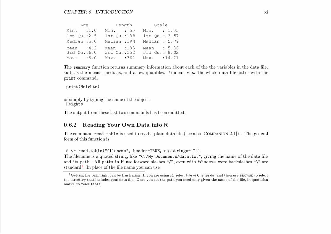
summary(wblake)
7/18/2019 Computing Primer for Applied Linear Regession by Weisberg
http://slidepdf.com/reader/full/computing-primer-for-applied-linear-regession-by-weisberg 12/153
CHAPTER 0. INTRODUCTION xi
Age Length Scale
Min. :1.0 Min. : 55 Min. : 1.05
1st Qu.:2.5 1st Qu.:138 1st Qu.: 3.57
Median :5.0 Median :194 Median : 5.79
Mean :4.2 Mean :193 Mean : 5.863rd Qu.:6.0 3rd Qu.:252 3rd Qu.: 8.02
Max. :8.0 Max. :362 Max. :14.71
The summary function returns summary information about each of the the variables in the data file,such as the means, medians, and a few quantiles. You can view the whole data file either with theprint command,
print(Heights)
or simply by typing the name of the object,Heights
The output from these last two commands has been omitted.
0.6.2 Reading Your Own Data into R
The command read.table is used to read a plain data file (see also Companion[2.1]) . The generalform of this function is:
d <- read.table("filename", header=TRUE, na.strings="?")
The filename is a quoted string, like "C:/My Documents/data.txt", giving the name of the data fileand its path. All paths in R use forward slashes “/”, even with Windows were backslashes “\” arestandard1. In place of the file name you can use
1Getting the path right can be frustrating. If you are using R, select File→Change dir, and then use browse to select
the directory that includes your data file. Once you set the path you need only given the name of the file, in quotation
marks, to read.table.

7/18/2019 Computing Primer for Applied Linear Regession by Weisberg
http://slidepdf.com/reader/full/computing-primer-for-applied-linear-regession-by-weisberg 13/153
CHAPTER 0. INTRODUCTION xii
d <- read.table(file.choose(), header=TRUE, na.strings="?")
in which case a standard file dialog will open and you can select the file you want in the usual way.The argument header=TRUE indicates that the first line of the file has variable names (you would say
header=FALSE if this were not so, and then the program would assign variable names like X1, X2 andso on), and the na.strings="?" indicates that missing values, if any, are indicated by a question markrather than the default of NA used by R. read.table has many more options; type help(read.table)
to learn about them. R has a package called foreign that can be used to read files of other types.You can also read the data directly into R from the internet:
d <-read.table("http://users.stat.umn.edu/~sandy/alr4ed/data/Htwt.csv",
header=TRUE, sep=",")
You can get most of the data files in the book in this way by substituting the file’s name, appending
.csv, and using the rest of the web address shown. Of course this is unnecessary because all the datafiles are part of the alr4 package.R is case sensitive , which means that a variable called weight is different from Weight, which in
turn is different from WEIGHT. Also, the command read.table would be different from READ.TABLE.Path names are case-sensitive on Linux and Macintosh, but not on Windows.
Frustration Alert: Reading data into R or any other statistical package can be frustrating. Yourdata may have blank rows and/or columns you do not remember creating. Typing errors, substitutinga capital “O” in place of a zero, can turn a column into a text variable. Odd missing value indicatorslike N/A, or inconsistent missing value indicators, can cause trouble. Variable names with embeddedblanks or other non-standard characters like a hash-mark #, columns on a data file for comments, canalso cause problems. Just remember: it’s not you, this happens to everyone until they have read in afew data sets successfully.

7/18/2019 Computing Primer for Applied Linear Regession by Weisberg
http://slidepdf.com/reader/full/computing-primer-for-applied-linear-regession-by-weisberg 14/153
CHAPTER 0. INTRODUCTION xiii
0.6.3 Reading Excel Files
(see also Companion[2.1.3]) R is less friendly in working with Excel files2. The easiest approach is tosave your data as a “.csv” file , which is a plain text file, with the items in each row of the file separated
by commas. You can then read the “.csv” file with the command read.cvs,data <- read.csv("ais.csv", header=TRUE)
where once again the complete path to the file is required. There are other tools described in Compan-ion[2.1.3] for reading Excel spreadsheets directly.
0.6.4 Saving Text and Graphs
The easiest way to save printed output is to select it, copy to the clipboard, and paste it into an editoror word processing program. Be sure to use a monospaced-font like Courier so columns line up properly.
In R on Windows, you can select File→Save to file to save the contents of the text window to a file.The easiest way to save a graph in R on Windows or Macintosh is via the plot’s menu. Select
File→Save as→filetype, where filetype is the format of the graphics file you want to use. You cancopy a graph to the clipboard with a menu item, and then paste it into a word processing document.
In all versions of R, you can also save files using a relatively complex method of defining a device ,Companion[7.4], for the graph. For example,
pdf("myhist.pdf", horizontal=FALSE, height=5, width=5)
hist(rnorm(100))
dev.off()
defines a device of type pdf to be saved in the file “myhist.pdf” in the current directory. It will consistof a histogram of 100 normal random numbers. This device remains active until the dev.off commandcloses the device. The default with pdf is to save the file in “landscape,” or horizontal mode to fill the
2A package called xlsx that can read Excel files directly. The package foreign contains functions to read many other
types of files created by SAS, SPSS, Stata and others.
7/18/2019 Computing Primer for Applied Linear Regession by Weisberg
http://slidepdf.com/reader/full/computing-primer-for-applied-linear-regession-by-weisberg 15/153
CHAPTER 0. INTRODUCTION xiv
page. The argument horizontal=FALSE orients the graph vertically, and height and width to 5 makesthe plotting region a five inches by five inches square.
R has many devices available, including pdf, postscript, jpeg and others; see help(Devices)
for a list of devices, and then, for example, help(pdf) for a list of the (many) arguments to the pdf
command.
0.6.5 Normal, F , t and χ2 tables
alr does not include tables for looking up critical values and significance levels for standard distributionslike the t, F and χ2. These values can be computed with R or Microsoft Excel, or tables are easilyfound by googling for example t table.
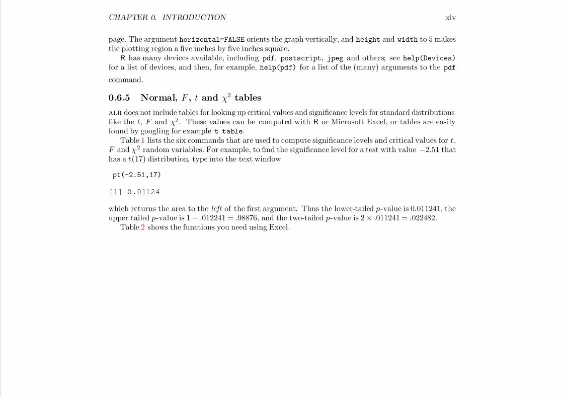
Table 1 lists the six commands that are used to compute significance levels and critical values for t,F and χ2 random variables. For example, to find the significance level for a test with value −2.51 thathas a t(17) distribution, type into the text window
pt(-2.51,17)
[1] 0.01124
which returns the area to the left of the first argument. Thus the lower-tailed p-value is 0.011241, theupper tailed p-value is 1 − .012241 = .98876, and the two-tailed p-value is 2 × .011241 = .022482.
Table 2 shows the functions you need using Excel.

7/18/2019 Computing Primer for Applied Linear Regession by Weisberg
http://slidepdf.com/reader/full/computing-primer-for-applied-linear-regession-by-weisberg 16/153
CHAPTER 0. INTRODUCTION xv
Table 1: Functions for computing p-values and critical values using R. These functions may have addi-tional arguments useful for other purposes.
Function What it doesqnorm(p) Returns a value q such that the area to the left of q for a
standard normal random variable is p.pnorm(q) Returns a value p such that the area to the left of q on a
standard normal is p.
qt(p, df) Returns a value q such that the area to the left of q on at(df) distribution equals q .pt(q, df) Returns p, the area to the left of q for a t(df ) distributionqf(p, df1, df2) Returns a value q such that the area to the left of q on a
F (df 1, df 2) distribution is p. For example, qf(.95, 3, 20)returns the 95% points of the F (3, 20) distribution.
pf(q, df1, df2) Returns p, the area to the left of q on a F (df 1,df 2) distri-bution.
qchisq(p, df) Returns a value q such that the area to the left of q on aχ2(df) distribution is p.
pchisq(q, df) Returns p, the area to the left of q on a χ2(df) distribution.

7/18/2019 Computing Primer for Applied Linear Regession by Weisberg
http://slidepdf.com/reader/full/computing-primer-for-applied-linear-regession-by-weisberg 17/153
CHAPTER 0. INTRODUCTION xvi
Table 2: Functions for computing p-values and critical values using Microsoft Excel. The definitions for thesefunctions are not consistent, sometimes corresponding to two-tailed tests, sometimes giving upper tails, andsometimes lower tails. Read the definitions carefully. The algorithms used to compute probability functionsin Excel are of dubious quality, but for the purpose of determining p-values or critical values, they should beadequate; see Knusel (2005) for more discussion.
Function What it does
normsinv(p) Returns a value q such that the area to the left of q for astandard normal random variable is p.
normsdist(q) The area to the left of q . For example, normsdist(1.96)
equals 0.975 to three decimals.tinv(p, df) Returns a value q such that the area to the left of −|q | and
the area to the right of +|q | for a t(df) distribution equalsq . This gives the critical value for a two-tailed test.
tdist(q, df, tails) Returns p, the area to the left of q for a t(df ) distributionif tails = 1, and returns the sum of the areas to the left of −|q | and to the right of +|q | if tails = 2, corresponding toa two-tailed test.
finv(p, df1, df2) Returns a value q such that the area to the right of q ona F (df 1, df 2) distribution is p. For example, finv(.05, 3,
20) returns the 95% point of the F (3, 20) distribution.fdist(q, df1, df2) Returns p, the area to the right of q on a F (df 1, df 2) distri-
bution.chiinv(p, df) Returns a value q such that the area to the right of q on a
χ2(df) distribution is p.chidist(q, df) Returns p, the area to the right of q on a χ2(df) distribution.

7/18/2019 Computing Primer for Applied Linear Regession by Weisberg
http://slidepdf.com/reader/full/computing-primer-for-applied-linear-regession-by-weisberg 18/153
CHAPTER 1
Scatterplots and Regression
1.1 Scatterplots
The plot function is R can be used with little fuss to produce pleasing scatterplots that can be used for
homework problems and for many other applications. You can get also get fancier graphs using someof plot’s many arguments; see Companion[Ch. 7].A simple scatterplot as in alr[F1.1a] is drawn by:
library(alr4)
plot(dheight ~ mheight, data=Heights)
1

7/18/2019 Computing Primer for Applied Linear Regession by Weisberg
http://slidepdf.com/reader/full/computing-primer-for-applied-linear-regession-by-weisberg 19/153
CHAPTER 1. SCATTERPLOTS AND REGRESSION 2
55 60 65 70
5 5
6 0
6 5
7 0
mheight
d h e i g h t
All the data in the alr4 are present after you use the library(alr4) command. The first argumentto the plot function is a formula, with the vertical or y-axis variable to the left of the ~ and thehorizontal or x-axis variable to the right. The argument data=Heights tells R to get the data from theHeights data frame.
This same graph can be obtained with other sets of arguments to plot:
plot(Heights$mheight, Heights$dheight)
This does not require naming the data frame as an argument, but does require the full name of thevariables to be plotted, including the name of the data frame. Variables or columns of a data frame arespecified using the $ notation in the above example.
with(Heights, plot(mheight, dheight))

7/18/2019 Computing Primer for Applied Linear Regession by Weisberg
http://slidepdf.com/reader/full/computing-primer-for-applied-linear-regession-by-weisberg 20/153
CHAPTER 1. SCATTERPLOTS AND REGRESSION 3
This uses the very helpful with function (Companion[2.2.2]), to specify the data frame to be used inthe the command that followed, in this case the plot command.
This plot command does not match alr[F1.1a] exactly, as the plot in the book included non-standard plotting characters, grid lines, a fixed aspect ratio of 1 and the same tick marks on both axes.
The script file for Chapter 1 gives the R commands to draw this plot. Companion[Ch. 7] describesmodification to R plots more generally.
alr[F1.1b] plots the rounded data:
plot(round(dheight) ~ round(mheight), Heights)
The figure alr[F1.2] is obtained from alr[F1.1a] by deleting most of the points. To draw this plotwe need to select points:
sel <- with(Heights,
(57.5 < mheight) & (mheight <= 58.5) |
(62.5 < mheight) & (mheight <= 63.5) |
(67.5 < mheight) & (mheight <= 68.5))
The result sel is a vector of values equal to either TRUE and FALSE. It is equal to TRUE if either57.5 < mheight ≤ 58.5, or 62.5 < mheight ≤ 63.5 or 67.5 < mheight ≤ 68.5. The vertical bar | is thelogical “or” operator; type help("|") to get the syntax for other logical operators.
We can redraw the figure using
plot(dheight ~ mheight, data=Heights, subset=sel)
The subset argument can be used with many R functions to specify which observations to use. Theargument can be (1) a list of TRUE and FALSE, as it is here, (2) a list of row numbers or row labels, or (3)if the argument were, for example, subset= -c(2, 5, 22), then all observations except row numbers2, 5, and 22 would be used. Since !sel would covert all TRUE to FALSE and all FALSE to TRUE, thespecification
plot(dheight ~ mheight, data=Heights, subset= !sel)

7/18/2019 Computing Primer for Applied Linear Regession by Weisberg
http://slidepdf.com/reader/full/computing-primer-for-applied-linear-regession-by-weisberg 21/153
CHAPTER 1. SCATTERPLOTS AND REGRESSION 4
would plot all the observations not in the specified ranges.alr[F1.3] adds several new features to scatterplots. the par function sets graphical parameters,
oldpar <- par(mfrow=c(1, 2))
meaning that the graphical window will hold an array of graphs with one row and two columns. Thischoice for the window will be kept until either the graphical window is closed or it is reset using anotherpar command. See ?par for all the graphical parameters (see also Companion[7.1.2]).
To draw alr[F1.3] we need to find the equation of the line to be drawn, and this is done usingthe lm command, the workhorse in R for fitting linear regression models. We will discuss this at muchgreater length in the next few chapters, but for now we will simply use the function.
m0 <- lm(pres ~ bp, data=Forbes)
plot(pres ~ bp, data=Forbes, xlab="Boiling Point (deg. F)",
ylab="Pressure (in Hg)")
abline(m0)plot(residuals(m0) ~ bp, Forbes, xlab="Boiling Point (deg. F)",
ylab="Residuals")
abline(a=0, b=0, lty=2)
par(oldpar)
The ols fit is computed using the lm function and assigned the name m0. The first plot draws thescatterplot of pres versus bp. We add the regression line with the function abline. When the argumentto abline is the name of a regression model, the function gets the information needed from the modelto draw the ols line. The second use of plot draws the second graph, this time of the residuals from
model m0 on the vertical axis versus bp on the horizontal axis. A horizontal dashed line is added to thisgraph by specifying intercept a equal to zero and slope b equal to zero. The argument lty=2 specifiesa dashed line; lty=1 would have given a solid line. The last command is unnecessary for drawing thegraph, but it returns the value of mfrow to its original state.
alr[F1.5] has two lines added to it, the ols line and the line joining the mean for each value of Age. First we use the tapply function (see also Companion[8.4]) to compute the mean Length foreach Age,

7/18/2019 Computing Primer for Applied Linear Regession by Weisberg
http://slidepdf.com/reader/full/computing-primer-for-applied-linear-regession-by-weisberg 22/153
CHAPTER 1. SCATTERPLOTS AND REGRESSION 5
(meanLength <- with(wblake, tapply(Length, Age, mean)))
1 2 3 4 5 6 7 8
98.34 124.85 152.56 193.80 221.72 252.60 269.87 306.25
Unpacking this complex command, (1) with is used to tell R to use the variables in the data framewblake; (2) the first argument of tapply is the variable of interest, the second argument gives thegrouping, and the third is the name of the function to be applied, here the mean function. The result issaved as an object called meanLength, and because we included parentheses around the whole expressionthe result is also printed on the screen.
plot(Age ~ Length, data=wblake)
abline(lm(Length ~ Age, data=wblake))
lines(1:8, meanLength, lty=2)
There are a few new features here. In the call to abline the regression was computed within thecommand, not in advance. The lines command adds lines to an existing plot, joining the pointsspecified. The points have horizontal coordinates 1:8, the integers from one to eight for the Age groups,and vertical coordinates given by meanLength as just computed.
alr[F1.7] adds a separate plotting character for each of the groups, and a legend. Here is how thiswas drawn in R:
plot(Gain ~ A, turkey, xlab="Amount (percent of diet)",
ylab="Weight gain (g)", pch=S)
legend("bottomright", inset=0.02, legend=c("1 Control", "2 New source A",
"3 New source B"), cex=0.75, lty=1:3, pch=1:3, lwd=c(1, 1.5, 2))
S is a variable in the data frame with the values 1, 2, or 3, so setting pch=S sets the plotting characterto be a the plotting characters that are associated with these numbers . Similarly, setting col=S will setthe color of the plotted points to be different for each of the three groups; try plot(1:20, pch=1:20,
col=1:20) to see the first 20 plotting characters and colors. The first argument to legend sets thelocation of the legend as the bottom right corner, and the inset argument insets the legend by 2%.

7/18/2019 Computing Primer for Applied Linear Regession by Weisberg
http://slidepdf.com/reader/full/computing-primer-for-applied-linear-regession-by-weisberg 23/153
CHAPTER 1. SCATTERPLOTS AND REGRESSION 6
The other arguments specify what goes in the legend. The lwd argument specifies the width of the linesdrawn in the legend.
1.4 Summary Graphalr[F1.9] was drawn using the xyplot function in the lattice package. You could get an almostequivalent plot using
oldpar <- par(mfrow=c(2, 2))
xs <- names(anscombe)[1:4]
ys <- names(anscombe)[5:8]
for (i in 1:4){
plot(anscombe[, xs[i]], anscombe[, ys[i]], xlab=xs[i], ylab=ys[i],
xlim=c(4,20), ylim=c(2, 16))
abline(lm( anscombe[, ys[i]] ~ anscombe[, xs[i]]))}
This introduced several new elements: (1) mfrow=c(2, 2) specified a 2 × 2 array of plots; (2) xs andys are, respectively, the names of the predictor and ther response for each of the four plot; (3) a loop,Companion[Sec. 8.3.2], was used to draw each of the plot; (4) columns of the data frame were accessedby their column numbers, or in this case by their column names; (5) labels and limits for the axes areset explicitly.
1.5 Tools for Looking at Scatterplotsalr[F1.10] adds a smoother to alr[F1.1a]. R has a wide variety of smoothers available, and all canbe added to a scatterplot. Here is how to add a loess smooth using the lowess function.
plot(dheight ~ mheight, Heights, cex=.1, pch=20)
abline(lm(dheight ~ mheight, Heights), lty=1)
with(Heights, lines(lowess(dheight ~ mheight, f=6/10, iter=1), lty=2))

7/18/2019 Computing Primer for Applied Linear Regession by Weisberg
http://slidepdf.com/reader/full/computing-primer-for-applied-linear-regession-by-weisberg 24/153
CHAPTER 1. SCATTERPLOTS AND REGRESSION 7
The lowess function specifies the response and predictor in the same way as lm. It also requires asmoothing parameter, which we have set to 0.6. The argument iter also controls the behavior of thesmoother; we prefer to set iter=1, not the default value of 3.
1.6 Scatterplot Matrices
The R function pairs draws scatterplot matrices. To reproduce an approximation to alr[F1.11], wemust first transform the data to get the variables that are to be plotted, and then draw the plot.
names(fuel2001)
[1] "Drivers" "FuelC" "Income" "Miles" "MPC" "Pop" "Tax"
fuel2001 <- transform(fuel2001,
Dlic=1000 * Drivers/Pop,
Fuel=1000 * FuelC/Pop,
Income = Income/1000)
names(fuel2001)
[1] "Drivers" "FuelC" "Income" "Miles" "MPC" "Pop" "Tax"
[8] "Dlic" "Fuel"
We used the transform function to add the transformed variables to the data frame. Variables that
reuse existing names, like Income, overwrite the existing variable. Variables with new names, like Dlic,are new columns added to the right of the data frame. The syntax for the transformations is similar tothe language C. The variable Dlic = 1000 × Drivers/Pop is the fraction of the population that has adriver’s license times 1000. We could have alternatively computed the transformations one at a time,for example
fuel2001$FuelPerDriver <- fuel2001$FuelC / fuel2001$Drivers

7/18/2019 Computing Primer for Applied Linear Regession by Weisberg
http://slidepdf.com/reader/full/computing-primer-for-applied-linear-regession-by-weisberg 25/153
CHAPTER 1. SCATTERPLOTS AND REGRESSION 8
Typing names(f) gives variable names in the order they appear in the data frame.The pairs function draws scatterplot matrices:
pairs(~ Tax + Dlic + Income + log(Miles) + Fuel, data=fuel2001)
We specify the variables we want to appear in the plot using a one-sided formula, which consists of a“ ~ ” followed by the variable names separated by + signs. The advantage of the one-sided formula isthat we can transform variables “on the fly” in the command, as we have done here using log(Miles)
rather than Miles.In the pairs command you could replace the formula with a matrix or data frame, so
pairs(fuel2001[, c(7, 9, 3, 6)])
would give the scatterplot matrix for columns 7, 9, 3, 6 of the data frame fuel2001.The function scatterplotMatrix in the car package provides a more elaborate version of scatterplot
matrices. The ?scatterplotMatrix, or Companion[3.3.2], can provide information.
1.7 Problems
1.1 R lets you plot transformed data without saving the transformed values:
plot(log(fertility) ~ log(ppgdp), UN11)
1.2 For the smallmouth bass data, you will need to compute the mean and sd of Length and sample
size for each value of Age. You can use tapply command three times for this, along with the mean, sd and length functions.
1.3 Use your mouse to change the aspect ratio in a plot by changing the shape of the plot’s window.

7/18/2019 Computing Primer for Applied Linear Regession by Weisberg
http://slidepdf.com/reader/full/computing-primer-for-applied-linear-regession-by-weisberg 26/153
CHAPTER 2
Simple Linear Regression
Most of alr[Ch. 2] fits simple linear regression from a few summary statistics, and we show how todo that using R below. While this is useful for understanding how simple regression works, in practicea higher-level function will be used to fit regression models. In R, this is the function lm (see alsoCompanion[Ch. 4]).
For the Forbes data used in the chapter, the simple regression model can be fit using
m1 <- lm(lpres ~ bp, data=Forbes)
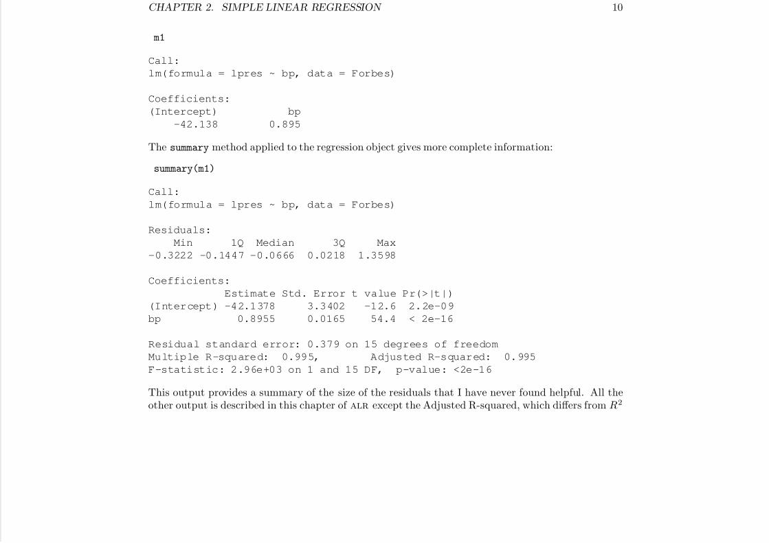
The first argument to lm is a formula. Here lpres ~ bp uses the name on the left of the ˜ as theresponse and the name or names to the right as predictors. The data argument tells R where to find thedata. Because of the assignment <- the result of this command is assigned the value m1, but nothing isprinted. If you print this object, you get the coefficient estimates:
9
7/18/2019 Computing Primer for Applied Linear Regession by Weisberg
http://slidepdf.com/reader/full/computing-primer-for-applied-linear-regession-by-weisberg 27/153
CHAPTER 2. SIMPLE LINEAR REGRESSION 10
m1
Call:
lm(formula = lpres ~ bp, data = Forbes)
Coefficients:
(Intercept) bp
-42.138 0.895
The summary method applied to the regression object gives more complete information:
summary(m1)
Call:
lm(formula = lpres ~ bp, data = Forbes)
Residuals:
Min 1Q Median 3Q Max
-0.3222 -0.1447 -0.0666 0.0218 1.3598
Coefficients:
Estimate Std. Error t value Pr(>|t|)
(Intercept) -42.1378 3.3402 -12.6 2.2e-09
bp 0.8955 0.0165 54.4 < 2e-16
Residual standard error: 0.379 on 15 degrees of freedom
Multiple R-squared: 0.995, Adjusted R-squared: 0.995
F-statistic: 2.96e+03 on 1 and 15 DF, p-value: <2e-16
This output provides a summary of the size of the residuals that I have never found helpful. All theother output is described in this chapter of alr except the Adjusted R-squared, which differs from R2

7/18/2019 Computing Primer for Applied Linear Regession by Weisberg
http://slidepdf.com/reader/full/computing-primer-for-applied-linear-regession-by-weisberg 28/153
CHAPTER 2. SIMPLE LINEAR REGRESSION 11
by a function of the sample size, and the F-statistic, which is discussed in Chapter 6. The Residual
standard error is σ.The object m1 created above includes many other quantities you may find useful:
names(m1)
[1] "coefficients" "residuals" "effects" "rank"
[5] "fitted.values" "assign" "qr" "df.residual"
[9] "xlevels" "call" "terms" "model"
Some of these are pretty obvious, like
m1$coefficients
(Intercept) bp
-42.1378 0.8955
but others are perhaps more obscure. The help page help(lm) provides more information. Similarly,you can save the output from summary as an object:
s1 <- summary(m1)
names(s1)
[1] "call" "terms" "residuals" "coefficients"
[5] "aliased" "sigma" "df" "r.squared"
[9] "adj.r.squared" "fstatistic" "cov.unscaled"
Some of these are obvious, such as s1$r.squared, and others not so obvious; print them to see whatthey are!

7/18/2019 Computing Primer for Applied Linear Regession by Weisberg
http://slidepdf.com/reader/full/computing-primer-for-applied-linear-regession-by-weisberg 29/153
CHAPTER 2. SIMPLE LINEAR REGRESSION 12
2.2 Least Squares Criterion
All the sample computations shown in alr are easily reproduced in R. First, get the right variablesfrom the data frame, and compute means.
Forbes1 <- Forbes[, c(1, 3)] # select columns 1 and 3print(fmeans <- colMeans(Forbes1))
bp lpres
203.0 139.6
The colMeans function computes the mean of each column of a matrix or data frame; the rowMeansfunction does the same for row means.
Next, we need the sums of squares and cross-products, and R provides several tools for this. Sincethe sample covariance matrix is just (n
−1) times the matrix of sums of squares and cross-products, we
can use the function cov:
(fcov <- (17 - 1) * cov(Forbes1))
bp lpres
bp 530.8 475.3
lpres 475.3 427.8
Alternatively, the function scale can be used to subtract the mean from each column of a matrix ordata frame, and then crossprod can be used to get the cross-product matrix:
crossprod(scale(Forbes1, center=TRUE, scale=FALSE))
bp lpres
bp 530.8 475.3
lpres 475.3 427.8
C A S A G SS O

7/18/2019 Computing Primer for Applied Linear Regession by Weisberg
http://slidepdf.com/reader/full/computing-primer-for-applied-linear-regession-by-weisberg 30/153
CHAPTER 2. SIMPLE LINEAR REGRESSION 13
All the regression summaries depend only on the sample means and on the sample sums of squaresfcov just computed. Assign names to the components to match the discussion in alr, and do thecomputations:
xbar <- fmeans[1]
ybar <- fmeans[2]SXX <- fcov[1,1]
SXY <- fcov[1,2]
SYY <- fcov[2,2]
betahat1 <- SXY/SXX
betahat0 <- ybar - betahat1 * xbar
print(c(betahat0 = betahat0, betahat1 = betahat1),
digits = 4)
betahat0.lpres betahat1-42.1378 0.8955
The collect function c was used to collect the output into a vector for nice printing. Compare to theestimates from lm given previously.
2.3 Estimating the Variance σ2
We can use the summary statistics computed previously to get the RSS and the estimate of σ2:
RSS <- SYY - SXY^2/SXXsigmahat2 <- RSS/15
sigmahat <- sqrt(sigmahat2)
c(RSS=RSS, sigmahat2=sigmahat2, sigmahat=sigmahat)
RSS sigmahat2 sigmahat
2.1549 0.1437 0.3790
CHAPTER 2 SIMPLE LINEAR REGRESSION 14

7/18/2019 Computing Primer for Applied Linear Regession by Weisberg
http://slidepdf.com/reader/full/computing-primer-for-applied-linear-regession-by-weisberg 31/153
CHAPTER 2. SIMPLE LINEAR REGRESSION 14
Using the regression object:
c(RSS = m1$df.residual * sigmaHat(m1)^2,
sigmathat2= sigmaHat(m1)^2,
sigmahat = sigmaHat(m1))
RSS sigmathat2 sigmahat
2.1549 0.1437 0.3790
The sigmaHat is a helper function is in the car package. It takes a regression object as its argument,and returns σ.
2.5 Estimated Variances
The standard errors of coefficient estimates can be computed from the fundamental quantities alreadygiven. The helper function vcov provides the variances and covariances of the estimated coefficients,
vcov(m1)
(Intercept) bp
(Intercept) 11.15693 -0.0549313
bp -0.05493 0.0002707
The diagonal elements are equal to the squared standard errors of the coefficient estimates and the
off-diagonal elements are the covariances between the coefficient estimates. You can turn this or anycovariance matrix into a correlation matrix:
cov2cor(vcov(m1))
(Intercept) bp
(Intercept) 1.0000 -0.9996
bp -0.9996 1.0000
CHAPTER 2 SIMPLE LINEAR REGRESSION 15

7/18/2019 Computing Primer for Applied Linear Regession by Weisberg
http://slidepdf.com/reader/full/computing-primer-for-applied-linear-regession-by-weisberg 32/153
CHAPTER 2. SIMPLE LINEAR REGRESSION 15
This is the matrix of correlations between the estimates.You can also extract the standard errors from the vcov output, but the method is rather obscure:
(ses <- sqrt(diag(vcov(m1))))
(Intercept) bp3.34020 0.01645
This used the sqrt function for square roots and the diag function to extract the diagonal elements of a matrix. The result is a vector, in this case of length 2.
2.6 Confidence Intervals and t-Tests
Confidence intervals and tests can be computed using the formulas in alr[2.6], in much the same wayas the previous computations were done.
To use lm we need the estimates and their standard errors ses previously computed. The last itemwe need to compute confidence intervals is the correct multiplier from the t distribution. For a 95%interval, the multiplier is
(tval <- qt(1-.05/2, m1$df))
[1] 2.131
The qt command computes quantiles of the t-distribution; similar function are available for the normal(qnorm), F (qF), and other distributions; see Section 0.6.5. The function qt finds the value tval sothat the area to the left of tval is equal to the first argument to the function. The second argument isthe degrees of freedom, which can be obtained from m1 as shown above.
Finally, the confidence intervals for the two estimates are:
betahat <- c(betahat0, betahat1)
data.frame(Est = betahat,
lower=betahat - tval * ses,
upper=betahat + tval * ses)
CHAPTER 2 SIMPLE LINEAR REGRESSION 16

7/18/2019 Computing Primer for Applied Linear Regession by Weisberg
http://slidepdf.com/reader/full/computing-primer-for-applied-linear-regession-by-weisberg 33/153
CHAPTER 2. SIMPLE LINEAR REGRESSION 16
Est lower upper
lpres -42.1378 -49.2572 -35.0183
0.8955 0.8604 0.9306
By creating a data frame, the values get printed in a nice table.
R includes a function called confint that computes the confidence intervals for you, and
confint(m1, level=.95)
2.5 % 97.5 %
(Intercept) -49.2572 -35.0183
bp 0.8604 0.9306
gives the same answer computed above. The confint function works with many other models in R, andis the preferred way to compute confidence intervals. For other than linear regression, it uses a moresophisticated method for computing confidence intervals.
Getting tests rather than intervals is similar.
2.7 The Coefficient of Determination, R2
For simple regression R2 is just the square of the correlation between the predictor and the response.It can be computed as in alr, or using the cor function,
SSreg <- SYY - RSS
print(R2 <- SSreg/SYY)
[1] 0.995
cor(Forbes1)
bp lpres
bp 1.0000 0.9975
lpres 0.9975 1.0000
CHAPTER 2 SIMPLE LINEAR REGRESSION 17

7/18/2019 Computing Primer for Applied Linear Regession by Weisberg
http://slidepdf.com/reader/full/computing-primer-for-applied-linear-regession-by-weisberg 34/153
CHAPTER 2. SIMPLE LINEAR REGRESSION 17
and 0.997478172 = 0.9949627.
Prediction and Fitted Values
Predictions and fitted values can be fairly easily computed given the estimates of the coefficients. Forexample, predictions at the original values of the predictor are given by
betahat0 + betahat1 * Forbes$bp
[1] 132.0 131.9 135.1 135.5 136.4 136.9 137.8 137.9 138.2 138.1 140.2 141.1
[13] 145.5 144.7 146.5 147.6 147.9
The predict command is a very powerful helper function for getting fitted and predictions from amodel fit with lm, or, indeed, most other models in R. Here are the important arguments1:
predict(object, newdata, se.fit = FALSE,interval = c("none", "confidence", "prediction"),
level = 0.95)
The object argument is the name of the regression model that has already been computed. Thenewdata argument is a data frame of values for which you want predictions or fitted values; if omittedthe default is the data used to fit the model. The interval argument specifies the type of interval youwant to compute. Three values are shown and any other value for this argument will produce an error.The default is "none", the first option shown. The level of the intervals will be 95% unless the level
argument is changed.In the simplest case, we have
predict(m1)
1You can see all the arguments by typing args(predict.lm).
CHAPTER 2. SIMPLE LINEAR REGRESSION 18

7/18/2019 Computing Primer for Applied Linear Regession by Weisberg
http://slidepdf.com/reader/full/computing-primer-for-applied-linear-regession-by-weisberg 35/153
CHAPTER 2. SIMPLE LINEAR REGRESSION 18
1 2 3 4 5 6 7 8 9 10 11 12 13
132.0 131.9 135.1 135.5 136.4 136.9 137.8 137.9 138.2 138.1 140.2 141.1 145.5
14 15 16 17
144.7 146.5 147.6 147.9
returning the fitted values (or predictions) for each observation. If you want predictions for particularvalues, say bp = 210 and 220, use the command
predict(m1, newdata=data.frame(bp=c(210,220)),
interval="prediction", level=.95)
fit lwr upr
1 145.9 145.0 146.8
2 154.9 153.8 155.9
The newdata argument is a powerful tool in using the predict command, as it allows computingpredictions at arbitrary points. The argument must be a data frame, with variables having the samenames as the variables used in the mean function. For the Forbes data, the only term beyond theintercept is for bp, and so only values for bp must be provided. The argument intervals="prediction"
gives prediction intervals at the specified level in addition to the point predictions; other intervals arepossible, such as for fitted values; see help(predict.lm) for more information.
Additional arguments to predict will compute additional quantities. For example, se.fit will alsoreturn the standard errors of the fitted values (not the standard error of prediction). For example,
predvals <- predict(m1, newdata=data.frame(bp=c(210, 220)),se.fit=TRUE)
predvals
$fit
1 2
145.9 154.9
CHAPTER 2. SIMPLE LINEAR REGRESSION 19

7/18/2019 Computing Primer for Applied Linear Regession by Weisberg
http://slidepdf.com/reader/full/computing-primer-for-applied-linear-regession-by-weisberg 36/153
$se.fit
1 2
0.1480 0.2951
$df
[1] 15
$residual.scale
[1] 0.379
The result predvals is a list (Companion[2.3.3] ). You could get a more compact representation bytyping
as.data.frame(predvals)
fit se.fit df residual.scale
1 145.9 0.1480 15 0.379
2 154.9 0.2951 15 0.379
You can do computations with these values. For example,
(150 - predvals$fit)/predvals$se.fit
1 2
27.6 -16.5
computes the difference between 150 and the fitted values, and then divides each by its standard errorof the fitted value. The predict helper function does not compute the standard error of prediction,but you can compute it using equation alr[E2.26],
se.pred <- sqrt(predvals$residual.scale^2 + predvals$se.fit^2)
CHAPTER 2. SIMPLE LINEAR REGRESSION 20

7/18/2019 Computing Primer for Applied Linear Regession by Weisberg
http://slidepdf.com/reader/full/computing-primer-for-applied-linear-regession-by-weisberg 37/153
2.8 The Residuals
The command residuals computes the residuals for a model. A plot of residuals versus fitted valueswith a horizontal line at 0 on the vertical axis is given by
plot(predict(m1), residuals(m1))abline(h=0,lty=2)
We will have more elaborate uses of residuals later in the Primer . If you apply the plot helperfunction to the regression model m1 by typing plot(m1), you will also get the plot of residuals versusfitted values, along with a few other plots that are not discussed in alr. Finally, the car functionresidualPlots can also be used:
residualPlots(m1)
We will discuss this last function in Chapter 9 of this primer.
2.9 Problems
2.1 The point of this problem is to get you to fit a regression “by hand”, basically by using R as agraphing calculator. For 2.1.1, use the plot function. For 2.1.2, you can compute the summarystatistics and the estimates as described earlier in primer. You can the the fitted line to your plotusing the abline function. For 2.1.3, compute the statistics using the formulas, and compare tothe values from the output of lm for these data.
2.4 Use the abline to add lines to a plot. An easy way to identify points in a plot is to use theidentify command:
plot(bigmac2009 ~ bigmac2003, UBSprices)
identify(UBSprices$bigmac2003, UBSprices$bigmac2009, rownames(UBSprices))
CHAPTER 2. SIMPLE LINEAR REGRESSION 21

7/18/2019 Computing Primer for Applied Linear Regession by Weisberg
http://slidepdf.com/reader/full/computing-primer-for-applied-linear-regession-by-weisberg 38/153
You can then click on the plot, and the label of the nearest point will be added to the plot.To stop identifying, either click the right mouse button and select “Stop”, or select
“Stop” from the plot’s menu.
2.7 You can add a new variable u1 to the data set:
Forbes$u1 <- 1/( (5/9)*Forbes$bp + 255.37)
For 2.7.4 you need to fit the same model to both the Forbes and Hooker data sets. You can thenuse the predict command to get the predictions for Hooker’s data from the fit to Forbes’ data,and vice versa .
2.10 In the cathedral data file for Problem 2.10.6 the variable Type is a text variable. You can turna text variable into a numeric variable with values 1 and 2 using
cathedral$group <- as.numeric(cathedral$Type)
If you want a variable of 0s and 1s, use
cathedral$group <- as.numeric(cathedral$Type) - 1
To do the problem you need to delete the last 7 rows of the file. Find out how many rows thereare:
dim(cathedral)
[1] 25 4
and then delete the last 7:
cathedral1 <- cathedral[-(19:25), ]
Here (19:25) generates the integers from 19 to 25, and the minus sign tells R to remove theserows. Specific columns, the second subscript, are not given, so the default is to use all the columns.
CHAPTER 2. SIMPLE LINEAR REGRESSION 22

7/18/2019 Computing Primer for Applied Linear Regession by Weisberg
http://slidepdf.com/reader/full/computing-primer-for-applied-linear-regession-by-weisberg 39/153
2.14 Use the sample function to to get the construction sample:
construction.sample <- sample(1:dim(Heights)[1], floor(dim(Heights)[1]/3))
This will choose the rows to be in the construction sample. Then, fit
m1 <- lm(dheight ~ mheight, Heights, subset=construction.sample)
You can get predictions for the remaining (validation) sample, like this:
predict(m1, newdata = Heights[-construction.sample,])
2.17 The formula for regression through the origin explicitly removes the intercept, y ~ x - 1.

7/18/2019 Computing Primer for Applied Linear Regession by Weisberg
http://slidepdf.com/reader/full/computing-primer-for-applied-linear-regession-by-weisberg 40/153
CHAPTER 3
Multiple Regression
3.1 Adding a Term to a Simple Linear Regression Model
The added-variable plots show what happens when we add a second regressor to a simple regressionmodel. Here are the steps. First, fit the regression of the response on the first regressor, and keep the
residuals:
m1 <- lm(lifeExpF ~ log(ppgdp), UN11)
r1 <- residuals(m1)
r1 is the part of the response not explained by the first regressor.Next, fit the regression of the second regressor on the first regressor and keep these residuals:
23
CHAPTER 3. MULTIPLE REGRESSION 24

7/18/2019 Computing Primer for Applied Linear Regession by Weisberg
http://slidepdf.com/reader/full/computing-primer-for-applied-linear-regession-by-weisberg 41/153
m2 <- lm(fertility ~ log(ppgdp), UN11)
r2 <- residuals(m2)
r2 is the part of the second regressor that is not explained by the first regressor.The added variable plot is r1 versus r2. The regression associated with the added variable plot:
m4 <- lm(resid(m1) ~ resid(m2))
has intercept 0, slope equal to the slope for the second regressor in the regression with two regressors,and the other properties described in alr. The resid function is the same as the residuals function.
3.1.1 Explaining Variability
3.1.2 Added-Variable Plots
The avPlots function in the car package can be used to draw added-variable plots. Introducing thisfunction here is a little awkward because it requires fitting a regression model first, a topic covered laterin this chapter.
library(alr4)
m3 <- lm(lifeExpF ~ log(ppgdp) + fertility, data=UN11)
avPlots(m3, id.n=0)
The first command loads the alr4 package, which in turn loads the car. The next command sets up thelinear regression model using lm; the only new feature is the formula has two terms on the right rather
than one. The avPlots function in the car package takes the regression model as its first argument.The default of the function is to display the added-variable plot for each variable on the right side of the formula, so we get two plots here. The argument id.n=0 is used to suppress point labeling . Bydefault avPlots will label several extreme points in the plot using row labels. In these plots they arerather distracting because the country names are long relative to the size of the graph.
Added-variable plots are discussed in Companion[6.2.3]. Point labeling is discussed in Compan-ion[3.5].
CHAPTER 3. MULTIPLE REGRESSION 25

7/18/2019 Computing Primer for Applied Linear Regession by Weisberg
http://slidepdf.com/reader/full/computing-primer-for-applied-linear-regession-by-weisberg 42/153
−3 −2 −1 0 1 2 3
− 2 0
− 1 0
0
5
1 0
log(ppgdp) | others
l i f e
E x p F
| o t h e r s
−2 −1 0 1 2 3
− 2 0
− 1 0
0
1 0
fertility | others
l i f e
E x p F
| o t h e r s
Added−Variable Plots
Figure 3.1: Added-variable plots for each of the two regressors in the regression of lifeExpF onlog(PPgdp)) and fertility.
CHAPTER 3. MULTIPLE REGRESSION 26

7/18/2019 Computing Primer for Applied Linear Regession by Weisberg
http://slidepdf.com/reader/full/computing-primer-for-applied-linear-regession-by-weisberg 43/153
3.2 The Multiple Linear Regression Model
3.3 Regressors and Predictors
All of the types of regressors created from predictros described in alr are easy to create and use in R.For now we discuss only a few of them:
Transformations of predictors Often you can create a transformation in a fitted model withoutactually adding the transformed values to a data file. For example, if you have a data frame called mydata with variables y, x1 and x2, you can compute the regression with terms x1 and log(x2)
by either of the following:
m1 <- lm(y ~ x1 + log(x2), mydata)
mydata <- transform(mydata, logx2=log(x2))
m2 <- lm(y ~ x1 + logx2, mydata)
The first form is preferable because R will recognize the x2 as the predictor rather than logx2 asthe predictor. The transform function added the transformed value to mydata. If you want touse the 1/y as the response, you could fit
m3 <- lm(I(1/y) ~ x1 + log(x2), mydata)
The identity function I forces the evaluation of its contents using usual arithmetic, rather thantreating the slash / using its special meaning in formulas.
Polynomials can be formed using the I function:
m4 <- lm( y ~ x1 + I(x1^2) + I(x1^3), mydata)
Even better is to use the poly function:
m4 <- lm( y ~ poly(x1, 3, raw=TRUE), mydata)
CHAPTER 3. MULTIPLE REGRESSION 27

7/18/2019 Computing Primer for Applied Linear Regession by Weisberg
http://slidepdf.com/reader/full/computing-primer-for-applied-linear-regession-by-weisberg 44/153
If you don’t set raw=TRUE the poly function creates orthogonal polynomials with superior numer-ical properties, alr[5.3].
Table 3.1 in alr[3.3] gives the “usual” summary statistics for each of the interesting terms in a dataframe. Oddly enough, the writers of R don’t seem to think these are the standard summaries. Here is
what you get from R:
fuel2001 <- transform(fuel2001,
Dlic=1000 * Drivers/Pop,
Fuel=1000 * FuelC/Pop,
Income = Income,
logMiles = log(Miles))
f <- fuel2001[,c(7, 8, 3, 10, 9)] # new data frame
summary(f)
Tax Dlic Income logMiles FuelMin. : 7.5 Min. : 700 Min. :20993 Min. : 7.34 Min. :318
1st Qu.:18.0 1st Qu.: 864 1st Qu.:25323 1st Qu.:10.51 1st Qu.:575
Median :20.0 Median : 909 Median :27871 Median :11.28 Median :626
Mean :20.2 Mean : 904 Mean :28404 Mean :10.91 Mean :613
3rd Qu.:23.2 3rd Qu.: 943 3rd Qu.:31208 3rd Qu.:11.63 3rd Qu.:667
Max. :29.0 Max. :1075 Max. :40640 Max. :12.61 Max. :843
We created a new data frame f using only the variables of interest. Rather than giving the standard
deviation for each variable, the summary command provides first and third quartiles. You can get thestandard deviations easily enough, using
apply(f, 2, sd)
Tax Dlic Income logMiles Fuel
4.545 72.858 4451.637 1.031 88.960
CHAPTER 3. MULTIPLE REGRESSION 28
7/18/2019 Computing Primer for Applied Linear Regession by Weisberg
http://slidepdf.com/reader/full/computing-primer-for-applied-linear-regession-by-weisberg 45/153
The apply function tells the program to apply the third argument, the sd function, to the seconddimension, or columns, of the matrix or data frame given by the first argument. We are not the first towonder why R doesn’t compute SDs in the summary command. The psych package, which you wouldneed to install from CRAN, contains a function called describe that will compute the usual summarystatistics and some unusual ones too!
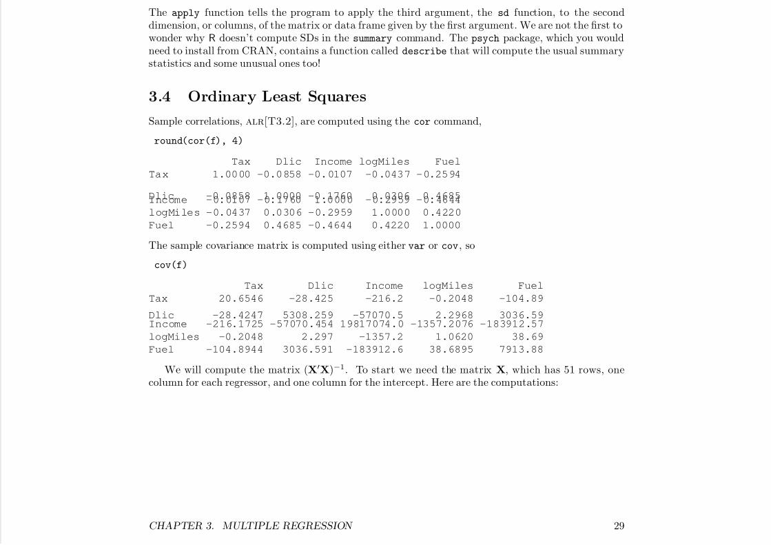
3.4 Ordinary Least Squares
Sample correlations, alr[T3.2], are computed using the cor command,
round(cor(f), 4)
Tax Dlic Income logMiles Fuel
Tax 1.0000 -0.0858 -0.0107 -0.0437 -0.2594
Dlic -0.0858 1.0000 -0.1760 0.0306 0.4685Income -0.0107 -0.1760 1.0000 -0.2959 -0.4644
logMiles -0.0437 0.0306 -0.2959 1.0000 0.4220
Fuel -0.2594 0.4685 -0.4644 0.4220 1.0000
The sample covariance matrix is computed using either var or cov, so
cov(f)
Tax Dlic Income logMiles Fuel
Tax 20.6546 -28.425 -216.2 -0.2048 -104.89
Dlic -28.4247 5308.259 -57070.5 2.2968 3036.59Income -216.1725 -57070.454 19817074.0 -1357.2076 -183912.57
logMiles -0.2048 2.297 -1357.2 1.0620 38.69
Fuel -104.8944 3036.591 -183912.6 38.6895 7913.88
We will compute the matrix (X′X)−1. To start we need the matrix X, which has 51 rows, onecolumn for each regressor, and one column for the intercept. Here are the computations:
CHAPTER 3. MULTIPLE REGRESSION 29
7/18/2019 Computing Primer for Applied Linear Regession by Weisberg
http://slidepdf.com/reader/full/computing-primer-for-applied-linear-regession-by-weisberg 46/153
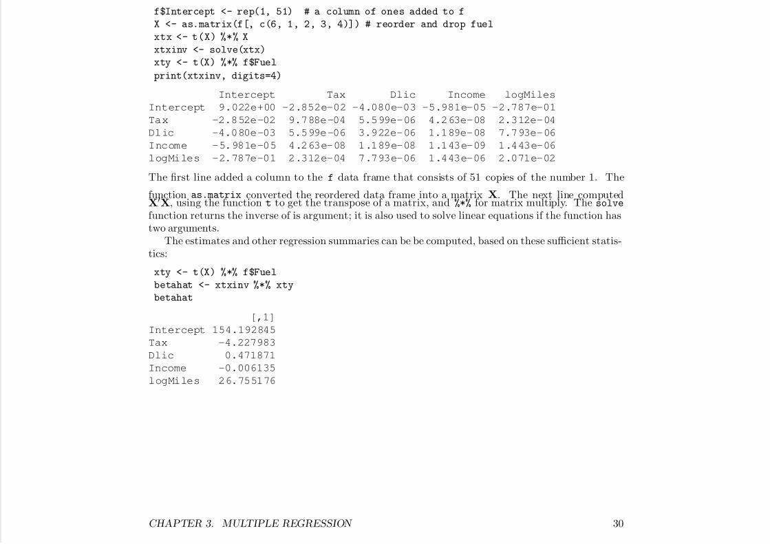
f$Intercept <- rep(1, 51) # a column of ones added to f
X <- as.matrix(f[, c(6, 1, 2, 3, 4)]) # reorder and drop fuel
xtx <- t(X) %*% X
xtxinv <- solve(xtx)
xty <- t(X) %*% f$Fuel
print(xtxinv, digits=4)
Intercept Tax Dlic Income logMiles
Intercept 9.022e+00 -2.852e-02 -4.080e-03 -5.981e-05 -2.787e-01
Tax -2.852e-02 9.788e-04 5.599e-06 4.263e-08 2.312e-04
Dlic -4.080e-03 5.599e-06 3.922e-06 1.189e-08 7.793e-06
Income -5.981e-05 4.263e-08 1.189e-08 1.143e-09 1.443e-06
logMiles -2.787e-01 2.312e-04 7.793e-06 1.443e-06 2.071e-02
The first line added a column to the f data frame that consists of 51 copies of the number 1. The
function as.matrix converted the reordered data frame into a matrix X. The next line computedX′X, using the function t to get the transpose of a matrix, and %*% for matrix multiply. The solve
function returns the inverse of is argument; it is also used to solve linear equations if the function hastwo arguments.
The estimates and other regression summaries can be be computed, based on these sufficient statis-tics:
xty <- t(X) %*% f$Fuel
betahat <- xtxinv %*% xty
betahat
[,1]
Intercept 154.192845
Tax -4.227983
Dlic 0.471871
Income -0.006135
logMiles 26.755176
CHAPTER 3. MULTIPLE REGRESSION 30
7/18/2019 Computing Primer for Applied Linear Regession by Weisberg
http://slidepdf.com/reader/full/computing-primer-for-applied-linear-regession-by-weisberg 47/153
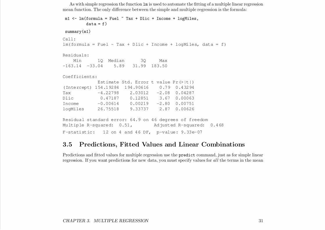
As with simple regression the function lm is used to automate the fitting of a multiple linear regressionmean function. The only difference between the simple and multiple regression is the formula:
m1 <- lm(formula = Fuel ~ Tax + Dlic + Income + logMiles,
data = f)
summary(m1)
Call:
lm(formula = Fuel ~ Tax + Dlic + Income + logMiles, data = f)
Residuals:
Min 1Q Median 3Q Max
-163.14 -33.04 5.89 31.99 183.50
Coefficients:
Estimate Std. Error t value Pr(>|t|)
(Intercept) 154.19284 194.90616 0.79 0.43294
Tax -4.22798 2.03012 -2.08 0.04287
Dlic 0.47187 0.12851 3.67 0.00063
Income -0.00614 0.00219 -2.80 0.00751
logMiles 26.75518 9.33737 2.87 0.00626
Residual standard error: 64.9 on 46 degrees of freedom
Multiple R-squared: 0.51, Adjusted R-squared: 0.468
F-statistic: 12 on 4 and 46 DF, p-value: 9.33e-07
3.5 Predictions, Fitted Values and Linear Combinations
Predictions and fitted values for multiple regression use the predict command, just as for simple linearregression. If you want predictions for new data, you must specify values for al l the terms in the mean
CHAPTER 3. MULTIPLE REGRESSION 31

7/18/2019 Computing Primer for Applied Linear Regession by Weisberg
http://slidepdf.com/reader/full/computing-primer-for-applied-linear-regession-by-weisberg 48/153
function, apart from the intercept, so for example,
predict(m1, newdata=data.frame(
Tax=c(20, 35), Dlic=c(909, 943), Income=c(16.3, 16.8),
logMiles=c(15, 17)))
1 2
899.8 905.9
will produce two predictions of future values for the values of the regressors indicated.
3.6 Problems
For these problems you will mostly be working with added-variable plots, outlined earlier, and working
with the lm function to do ols fitting. The helper functions predict get predictions, residuals getthe residuals, and confint compute confidence intervals for coefficient estimates.
7/18/2019 Computing Primer for Applied Linear Regession by Weisberg
http://slidepdf.com/reader/full/computing-primer-for-applied-linear-regession-by-weisberg 49/153
CHAPTER 4
Interpretation of Main Effects
4.1 Understanding Parameter Estimates
4.1.1 Rate of Change
alr[F4.1] is an example of an effects plot , used extensively in alr to help visualize the role of individualregressors in a fitted model. The idea is particularly simple when all the regressors in a regressionequation are predictors:
1. Get a fitted model likey = β 0 + β 1x1 + β 2x2 + · · · + β px p
32
CHAPTER 4. INTERPRETATION OF MAIN EFFECTS 33
7/18/2019 Computing Primer for Applied Linear Regession by Weisberg
http://slidepdf.com/reader/full/computing-primer-for-applied-linear-regession-by-weisberg 50/153
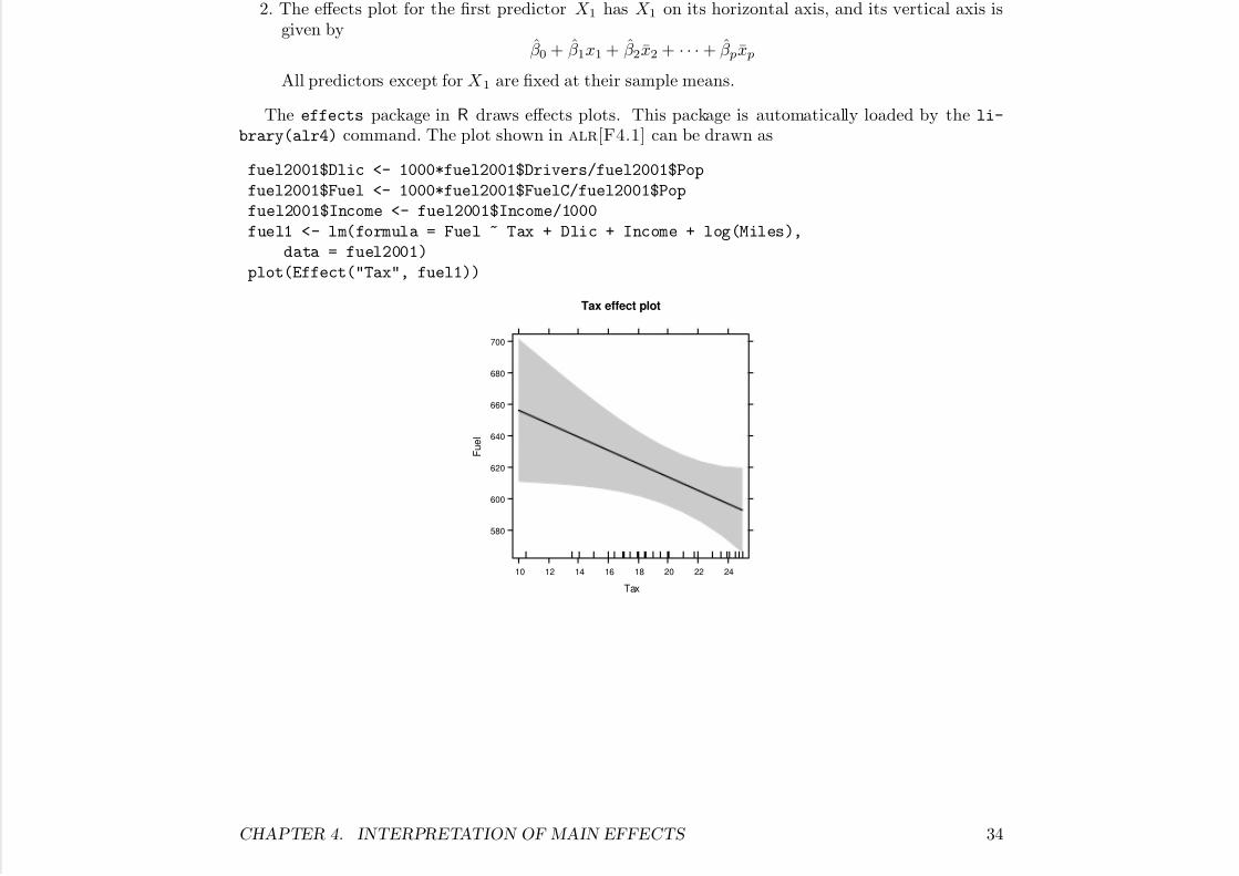
2. The effects plot for the first predictor X 1 has X 1 on its horizontal axis, and its vertical axis isgiven by
β 0 + β 1x1 + β 2x2 + · · · + β px p
All predictors except for X 1 are fixed at their sample means.
The effects package in R draws effects plots. This package is automatically loaded by the li-
brary(alr4) command. The plot shown in alr[F4.1] can be drawn as
fuel2001$Dlic <- 1000*fuel2001$Drivers/fuel2001$Pop
fuel2001$Fuel <- 1000*fuel2001$FuelC/fuel2001$Pop
fuel2001$Income <- fuel2001$Income/1000
fuel1 <- lm(formula = Fuel ~ Tax + Dlic + Income + log(Miles),
data = fuel2001)
plot(Effect("Tax", fuel1))
Tax effect plot
Tax
F u e l
580
600
620
640
660
680
700
10 12 14 16 18 20 22 24
CHAPTER 4. INTERPRETATION OF MAIN EFFECTS 34
7/18/2019 Computing Primer for Applied Linear Regession by Weisberg
http://slidepdf.com/reader/full/computing-primer-for-applied-linear-regession-by-weisberg 51/153
The first three lines above create the data set, the next line fits the regression model, and the next linedraws the plot. First, the Effect method is called with the name of the predictor of interest in quotes,here "Tax", and then the name of the regression model, here fuel1. The output from this function isthen input to the plot command, which is written to work with the output from Effect1 The curvedshaded area on the plot displays pointwise 95% confidence intervals.
4.1.3 Interpretation Depends on Other Terms in the Mean Function
In alr[T4.1], Model 3 is overparameterized. R will print the missing value symbol NA for regressors thatare linear combinations of the regressors already fit in the mean function, so they are easy to identifyfrom the printed output.
BGSgirls$DW9 <- BGSgirls$WT9-BGSgirls$WT2
BGSgirls$DW18 <- BGSgirls$WT18-BGSgirls$WT9
BGSgirls$DW218 <- BGSgirls$WT18-BGSgirls$WT2
m1 <- lm(BMI18 ~ WT2 + WT9 + WT18 + DW9 + DW18, BGSgirls)
m2 <- lm(BMI18 ~ WT2 + DW9 + DW18 + WT9 + WT18, BGSgirls)
m3 <- lm(BMI18 ~ WT2 + WT9 + WT18 + DW9 + DW18, BGSgirls)
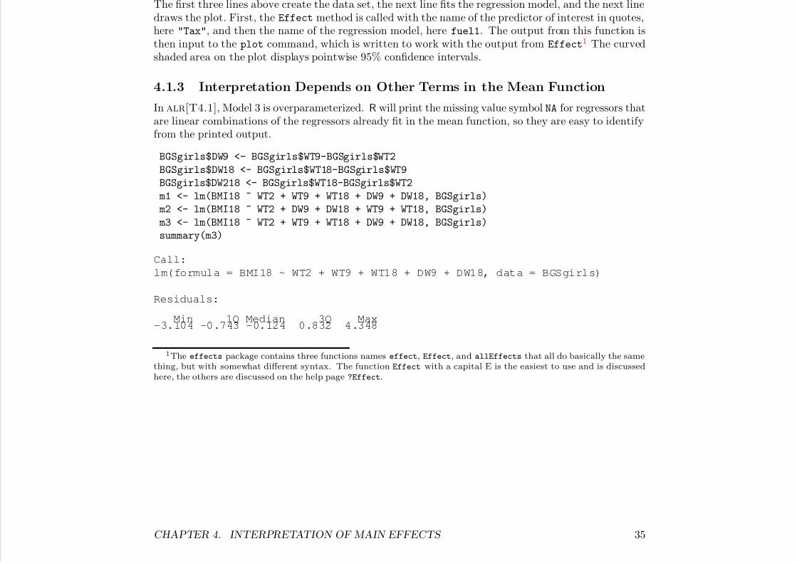
summary(m3)
Call:
lm(formula = BMI18 ~ WT2 + WT9 + WT18 + DW9 + DW18, data = BGSgirls)
Residuals:
Min 1Q Median 3Q Max-3.104 -0.743 -0.124 0.832 4.348
1The effects package contains three functions names effect, Effect, and allEffects that all do basically the same
thing, but with somewhat different syntax. The function Effect with a capital E is the easiest to use and is discussed
here, the others are discussed on the help page ?Effect.
CHAPTER 4. INTERPRETATION OF MAIN EFFECTS 35
7/18/2019 Computing Primer for Applied Linear Regession by Weisberg
http://slidepdf.com/reader/full/computing-primer-for-applied-linear-regession-by-weisberg 52/153
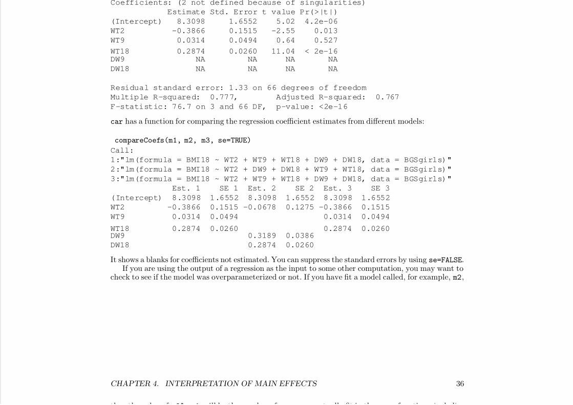
Coefficients: (2 not defined because of singularities)
Estimate Std. Error t value Pr(>|t|)
(Intercept) 8.3098 1.6552 5.02 4.2e-06
WT2 -0.3866 0.1515 -2.55 0.013
WT9 0.0314 0.0494 0.64 0.527
WT18 0.2874 0.0260 11.04 < 2e-16DW9 NA NA NA NA
DW18 NA NA NA NA
Residual standard error: 1.33 on 66 degrees of freedom
Multiple R-squared: 0.777, Adjusted R-squared: 0.767
F-statistic: 76.7 on 3 and 66 DF, p-value: <2e-16
car has a function for comparing the regression coefficient estimates from different models:
compareCoefs(m1, m2, m3, se=TRUE)
Call:
1:"lm(formula = BMI18 ~ WT2 + WT9 + WT18 + DW9 + DW18, data = BGSgirls)"
2:"lm(formula = BMI18 ~ WT2 + DW9 + DW18 + WT9 + WT18, data = BGSgirls)"
3:"lm(formula = BMI18 ~ WT2 + WT9 + WT18 + DW9 + DW18, data = BGSgirls)"
Est. 1 SE 1 Est. 2 SE 2 Est. 3 SE 3
(Intercept) 8.3098 1.6552 8.3098 1.6552 8.3098 1.6552
WT2 -0.3866 0.1515 -0.0678 0.1275 -0.3866 0.1515
WT9 0.0314 0.0494 0.0314 0.0494
WT18 0.2874 0.0260 0.2874 0.0260DW9 0.3189 0.0386
DW18 0.2874 0.0260
It shows a blanks for coefficients not estimated. You can suppress the standard errors by using se=FALSE.If you are using the output of a regression as the input to some other computation, you may want to
check to see if the model was overparameterized or not. If you have fit a model called, for example, m2,
CHAPTER 4. INTERPRETATION OF MAIN EFFECTS 36
th th l f 2$ k ill b th b f t ll fit i th f ti i l di

7/18/2019 Computing Primer for Applied Linear Regession by Weisberg
http://slidepdf.com/reader/full/computing-primer-for-applied-linear-regession-by-weisberg 53/153
then the value of m2$rank will be the number of regressors actually fit in the mean function, including the intercept, if any . It is also possible to determine which of the regressors specified in the meanfunction were actually fit, but the command for this is obscure:
> m2$qr$pivot[1:m2$qr$rank]
will return the indices of the regressors, starting with the intercept, that were estimated in fitting themodel.
4.1.5 Colinearity
For a set of regressors with observed values given by the columns of X, we diagnose colinearity if thesquare of the multiple correlation between one of the columns, say X 1 and the remaining columns, sayX2, R2
X1,X2, is large enough. A variance inflation factor is defined as v = 1/(1 − R2
X1,X2), and these
values are more often available in computer packages, including the vif command in the car package.
If v is a variance inflation factor, then (v − 1)/v is the corresponding value of the squared multiplecorrelation.
4.1.6 Regressors in Logarithmic Scale
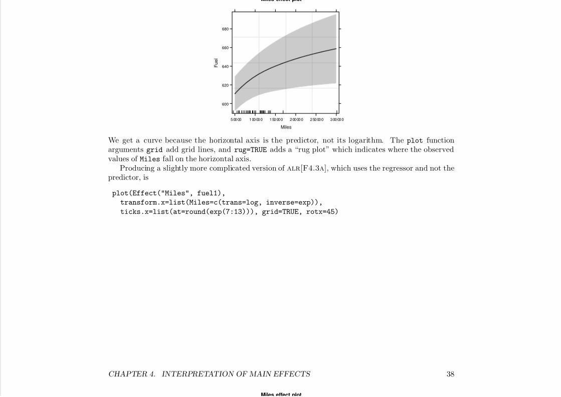
Effects plots should ordinarily be drawn using predictors, not the regressors created from them. Anexample is alr[F4.4b], drawn with the simple command
plot(Effect("Miles", fuel1), grid=TRUE, rug=TRUE)
CHAPTER 4. INTERPRETATION OF MAIN EFFECTS 37
Miles effect plot
7/18/2019 Computing Primer for Applied Linear Regession by Weisberg
http://slidepdf.com/reader/full/computing-primer-for-applied-linear-regession-by-weisberg 54/153
Miles effect plot
Miles
F u e l
600
620
640
660
680
50000 100000 150000 200000 250000 300000
We get a curve because the horizontal axis is the predictor, not its logarithm. The plot functionarguments grid add grid lines, and rug=TRUE adds a “rug plot” which indicates where the observedvalues of Miles fall on the horizontal axis.
Producing a slightly more complicated version of alr[F4.3a], which uses the regressor and not thepredictor, is
plot(Effect("Miles", fuel1),
transform.x=list(Miles=c(trans=log, inverse=exp)),
ticks.x=list(at=round(exp(7:13))), grid=TRUE, rotx=45)
CHAPTER 4. INTERPRETATION OF MAIN EFFECTS 38
Miles effect plot

7/18/2019 Computing Primer for Applied Linear Regession by Weisberg
http://slidepdf.com/reader/full/computing-primer-for-applied-linear-regession-by-weisberg 55/153
Miles effect plot
Miles
F u e l
600
620
640
660
680
5 0 0
0 0
1 0 0 0
0 0
1 5 0 0
0 0
2 0 0 0
0 0
2 5 0 0
0 0
3 0 0 0
0 0
The call to Effect is the same, but additional arguments are needed in the call to plot: transform.xtells to transform Miles on the horizontal axis to its logarithm; you must also specify the inverse of thelog-function. Finally, you need to tell the function where to draw the tick marks. Since log(Miles) isbetween about 7 and 13, the ticks are found by exponentiating these values and then rounding them.The argument rotx=45 rotates the labels on the horizontal axis by 45 degrees so the numbers do notoverlap. See ?plot.eff to see all the arguments.
4.6 Problems
4.1 To compute transformed values for this problem and the next problem, you can use statementslike this:
BGSgirls$ave <- with(BGSgirls, (WT9 + WT9 + WT18)/3)
CHAPTER 4. INTERPRETATION OF MAIN EFFECTS 39
4 11 4 11 1 To generate 100 standard normal random deviates:

7/18/2019 Computing Primer for Applied Linear Regession by Weisberg
http://slidepdf.com/reader/full/computing-primer-for-applied-linear-regession-by-weisberg 56/153
4.11 4.11.1 To generate 100 standard normal random deviates:
x <- rnorm(100)
To generate deviates with mean µ = 5 and standard deviation σ = 3,
x <- 5 + 3 * rnorm(100)
4.11.4 To fit a linear model excluding all cases with |x| < 2/3:
m1 <- lm(y ~ x, subset = abs(x) > 2/3)
To fit to only these cases, use
m2 <- update(m1, subset = !(abs(x) > 2/3))
The exclamation point is the same as “not”.

7/18/2019 Computing Primer for Applied Linear Regession by Weisberg
http://slidepdf.com/reader/full/computing-primer-for-applied-linear-regession-by-weisberg 57/153
CHAPTER 5
Complex Regressors
5.1 Factors
A factor is a qualitative variable with say a levels or groups. It will generally be represented by a− 1dummy variables. In models with no intercept, a dummy variables may be required. In alr[5.1.1] the
dummy variables are defined using the following rules:
1. If a factor A has a levels, create a dummy variables U 1, . . . , U a, such that U j has the value onewhen the level of A is j , and value zero everywhere else.
2. Obtain a set of a − 1 dummy variables to represent factor A by dropping one of the dummyvariables. Using the default coding in R, the first dummy variable U 1 is dropped, while in SAS
40
CHAPTER 5. COMPLEX REGRESSORS 41
and SPSS and STATA the last dummy variable is dropped.
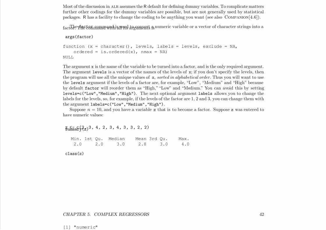
7/18/2019 Computing Primer for Applied Linear Regession by Weisberg
http://slidepdf.com/reader/full/computing-primer-for-applied-linear-regession-by-weisberg 58/153
y pp
Most of the discussion in alr assumes the R default for defining dummy variables. To complicate mattersfurther other codings for the dummy variables are possible, but are not generally used by statisticalpackages. R has a facility to change the coding to be anything you want (see also Companion[4.6]).
The factor command is used to convert a numeric variable or a vector of character strings into afactor. The command with all its arguments is
args(factor)
function (x = character(), levels, labels = levels, exclude = NA,
ordered = is.ordered(x), nmax = NA)
NULL
The argument x is the name of the variable to be turned into a factor, and is the only required argument.The argument levels is a vector of the names of the levels of x; if you don’t specify the levels, thenthe program will use all the unique values of x, sorted in alphabetical order . Thus you will want to usethe levels argument if the levels of a factor are, for example, “Low”, “Medium” and “High” becauseby default factor will reorder them as “High,” “Low” and “Medium.” You can avoid this by settinglevels=c("Low","Medium","High"). The next optional argument labels allows you to change thelabels for the levels, so, for example, if the levels of the factor are 1, 2 and 3, you can change them withthe argument labels=c("Low","Medium","High").
Suppose n = 10, and you have a variable z that is to become a factor. Suppose z was entered tohave numeric values:
z <- c(2, 3, 4, 2, 3, 4, 3, 3, 2, 2)summary(z)
Min. 1st Qu. Median Mean 3rd Qu. Max.
2.0 2.0 3.0 2.8 3.0 4.0
class(z)
CHAPTER 5. COMPLEX REGRESSORS 42
[1] "numeric"

7/18/2019 Computing Primer for Applied Linear Regession by Weisberg
http://slidepdf.com/reader/full/computing-primer-for-applied-linear-regession-by-weisberg 59/153
The class of z is numeric, regular numbers. The summary of a numeric vector includes the minimum,maximum, mean and other statistics.
You can convert z to a factor using
z.factor <- factor(z)
summary(z.factor)
2 3 4
4 4 2
class(z.factor)
[1] "factor"
The summary for a factor is the number of observations at each level. You can change the labels forthe levels of the factor:
z.factor <- factor(z, labels=c("Group1", "Group2", "Group3"))
summary(z.factor)
Group1 Group2 Group3
4 4 2
class(z.factor)
[1] "factor"
You can convert a factor back to a vector of numbers:
as.numeric(z.factor)
CHAPTER 5. COMPLEX REGRESSORS 43
[1] 1 2 3 1 2 3 2 2 1 1

7/18/2019 Computing Primer for Applied Linear Regession by Weisberg
http://slidepdf.com/reader/full/computing-primer-for-applied-linear-regession-by-weisberg 60/153
where the numbers are the level numbers, starting with 1.In the datasets in the alr4 factors will generally have been stored as factors, so you won’t need to
specify them as factors. You can always find out about a factor as follows:
class(UN11$group)
[1] "factor"
levels(UN11$group)
[1] "oecd" "other" "africa"
R uses the first level of a factor as a baseline group, but this is not always desirable. There are manyways to change this. Here are two alternatives that use the relevel and the factor commands.
levels(relevel(z.factor, "Group3"))
[1] "Group3" "Group1" "Group2"
levels(factor(z.factor, levels=c("Group2", "Group3", "Group1")))
[1] "Group2" "Group3" "Group1"
5.1.1 One-Factor Modelsalr[5.1] displays a boxplot with particular points labeled. The Boxplot function in the car package,with a capital “B”, makes this easy:
Boxplot(lifeExpF ~ group, data=UN11, id.n=2)
CHAPTER 5. COMPLEX REGRESSORS 44
The argument id.n=2 identifies up to 2 points in each boxplot and labels them. This argument isf f

7/18/2019 Computing Primer for Applied Linear Regession by Weisberg
http://slidepdf.com/reader/full/computing-primer-for-applied-linear-regession-by-weisberg 61/153
available in most of the plotting methods in the car package. The method that is used to identifypoints depends on the plot, and can be changed using other arguments. See ?showLabels.
Here is the code that generates the dummy variables for group for the first 10 rows of the UN11 data:
head(model.matrix(~ -1 + group, UN11), 10)
groupoecd groupother groupafrica
Afghanistan 0 1 0
Albania 0 1 0
Algeria 0 0 1
Angola 0 0 1
Anguilla 0 1 0
Argentina 0 1 0
Armenia 0 1 0
Aruba 0 1 0Australia 1 0 0
Austria 1 0 0
The magic command model.matrix returns the regressors generated by the variables in the formulagiven as its argument. By putting the -1 in the formula the intercept is excluded so all the dummyvariables for group are displayed. Try it without the -1. The head command prints the first few rowsof a matrix or data frame, here the first 10. There is also a tail command to print the last few, and asome command, in the car package, to print a few rows selected at random.
alr[F5.2] has lines fitted separately to each level of group. The scatterplot function in the car
package makes this easy:
scatterplot(lifeExpF ~ log(ppgdp)| group, data=UN11,
smooth=FALSE, boxplots=FALSE,
ylab="Female Life Expectancy")
CHAPTER 5. COMPLEX REGRESSORS 45
The plot is “conditioned on” the variable to the right of the |. scatterplot has defaults that weh d f t d h b l FALSE i l b l t h FALSE fitti

7/18/2019 Computing Primer for Applied Linear Regession by Weisberg
http://slidepdf.com/reader/full/computing-primer-for-applied-linear-regession-by-weisberg 62/153
have defeated here: boxplots=FALSE suppresses marginal boxplots; smooth=FALSE suppresses fittingsmoothers. Try drawing the plot without these two arguments (see also Companion[3.2.1]).
5.1.2 Adding a Continuous Predictor
Here is the R code that will give an approximation to alr[F5.3]. First, fit the regression model,
m1 <- lm(lifeExpF ~ group * log(ppgdp), UN11)
Then, draw the plot
plot(Effect(c("group", "ppgdp"), m1, default.levels=100),
rug=FALSE, grid=TRUE, multiline=TRUE)
The Effect function had as its first argument the names of two predictors, and it figured out that the
group*log(ppgdp) interaction is of interest.The plot in alr[F5.3b] requires changing the horizontal axis. The syntax for this is a little compli-
cated.
plot(Effect(c("group", "ppgdp"), m1, default.levels=100),
rug=FALSE, grid=TRUE, multiline=TRUE,
transform.x=list(ppgdp=list(trans=log, inverse=exp)),
ticks.x =list(at= c(100, 1000, 5000, 30000)))
5.1.3 The Main Effects ModelHere is the code for alr[F5.4].
plot(allEffects(m1, default.levels=50), ylim=c(60,85),
grid=TRUE, multiline=TRUE)
CHAPTER 5. COMPLEX REGRESSORS 46
The allEffects function results in plots being drawn for all relevant effects1 The ylim argumentguarantees that the the limits on the ertical a is are the same for each plot
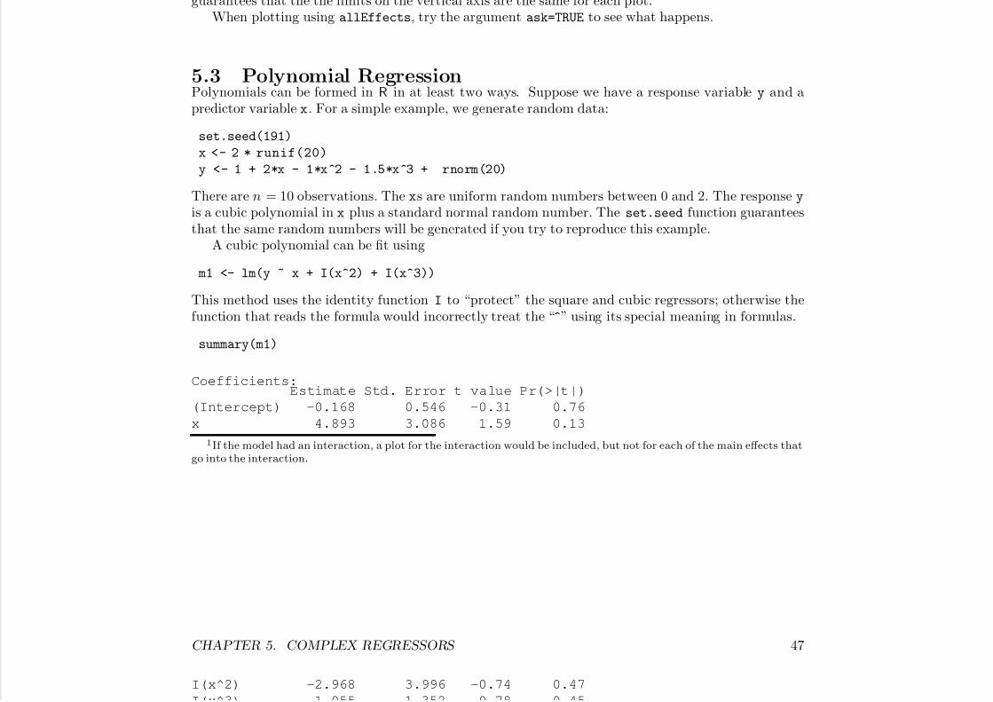
7/18/2019 Computing Primer for Applied Linear Regession by Weisberg
http://slidepdf.com/reader/full/computing-primer-for-applied-linear-regession-by-weisberg 63/153
guarantees that the the limits on the vertical axis are the same for each plot.When plotting using allEffects, try the argument ask=TRUE to see what happens.
5.3 Polynomial RegressionPolynomials can be formed in R in at least two ways. Suppose we have a response variable y and apredictor variable x. For a simple example, we generate random data:
set.seed(191)
x <- 2 * runif(20)
y <- 1 + 2*x - 1*x^2 - 1.5*x^3 + rnorm(20)
There are n = 10 observations. The xs are uniform random numbers between 0 and 2. The response y
is a cubic polynomial in x plus a standard normal random number. The set.seed function guaranteesthat the same random numbers will be generated if you try to reproduce this example.
A cubic polynomial can be fit using
m1 <- lm(y ~ x + I(x^2) + I(x^3))
This method uses the identity function I to “protect” the square and cubic regressors; otherwise thefunction that reads the formula would incorrectly treat the “^” using its special meaning in formulas.
summary(m1)
Coefficients:Estimate Std. Error t value Pr(>|t|)
(Intercept) -0.168 0.546 -0.31 0.76
x 4.893 3.086 1.59 0.13
1If the model had an interaction, a plot for the interaction would be included, but not for each of the main effects that
go into the interaction.
CHAPTER 5. COMPLEX REGRESSORS 47
I(x^2) -2.968 3.996 -0.74 0.47
I(x^3) 1 055 1 352 0 78 0 45

7/18/2019 Computing Primer for Applied Linear Regession by Weisberg
http://slidepdf.com/reader/full/computing-primer-for-applied-linear-regession-by-weisberg 64/153
I(x 3) -1.055 1.352 -0.78 0.45
Residual standard error: 0.922 on 16 degrees of freedom
Multiple R-squared: 0.941
F-statistic: 85.2 on 3 and 16 DF, p-value: 4.7e-10
An alternative approach is to use the function poly (see also Companion[4.6.3]):
summary(m2 <- lm(y ~ poly(x, 3, raw=TRUE)))
Coefficients:
Estimate Std. Error t value Pr(>|t|)
(Intercept) -0.168 0.546 -0.31 0.76
poly(x, 3, raw = TRUE)1 4.893 3.086 1.59 0.13
poly(x, 3, raw = TRUE)2 -2.968 3.996 -0.74 0.47poly(x, 3, raw = TRUE)3 -1.055 1.352 -0.78 0.45
Residual standard error: 0.922 on 16 degrees of freedom
Multiple R-squared: 0.941
F-statistic: 85.2 on 3 and 16 DF, p-value: 4.7e-10
An advantage to this second approach is that an effect plot can return the fitted cubic with the secondapproach but not with the first:
print(plot(Effect("x", m2)))
CHAPTER 5. COMPLEX REGRESSORS 48
x effect plot

7/18/2019 Computing Primer for Applied Linear Regession by Weisberg
http://slidepdf.com/reader/full/computing-primer-for-applied-linear-regession-by-weisberg 65/153
x
y
−4
−3
−2
−1
0
1
2
0.6 0.8 1.0 1.2 1.4
Setting raw=FALSE in poly uses orthogonal polynomials rather than raw polynomials, Compan-ion[4.6.3], alr[5.3.2]. The parameters are different, but the fitted values and the test for the cubicregressor are the same.
summary(m3 <- lm(y ~ poly(x, 3)))
Coefficients:
Estimate Std. Error t value Pr(>|t|)
(Intercept) -0.941 0.206 -4.56 0.00032
poly(x, 3)1 -11.113 0.922 -12.06 1.9e-09
poly(x, 3)2 -9.651 0.922 -10.47 1.4e-08
poly(x, 3)3 -0.719 0.922 -0.78 0 .44665
Residual standard error: 0.922 on 16 degrees of freedomMultiple R-squared: 0.941
F-statistic: 85.2 on 3 and 16 DF, p-value: 4.7e-10
CHAPTER 5. COMPLEX REGRESSORS 49
5.3.1 Polynomials with Several Predictors
(S l C [S ] ) h d d l h d

7/18/2019 Computing Primer for Applied Linear Regession by Weisberg
http://slidepdf.com/reader/full/computing-primer-for-applied-linear-regession-by-weisberg 66/153
(See also Companion[Sec. 4.6.3].) With two predictors, and generalizing to more than two predictors,the full second-order mean function alr[E6.4] can be fit to the cakes data by
m1 <- lm(Y ~ X1 + X2 + I(X1^2) + I(X2^2) + X1:X2, data=cakes)
or more compactly using the polym function
m2 <- lm(Y ~ polym(X1, X2, degree=2, raw=TRUE), data=cakes)
Try fitting both of these and compare the fitted models.The new feature here is the interaction regressor X1:X2, which is obtained by multiplying X1 by X2
elementwise. Other programs often write an interaction as X1*X2, but in R, X1*X2 = X1+X2+X1:X2.With the cakes data, try this command and see if you can figure out the meaning of all the variables.
model.matrix(~ polym(X1, X2, degree=2, raw=TRUE), data=cakes)
This matrix is hard to understand because of the very long column names. Here’s an alternative thatwill shorten the names:
z <- with(cakes, polym(X1, X2, degree=2, raw=TRUE))
model.matrix(~ z)
5.4 Splines
Splines are an advanced topic that you or your instructor may choose to skip at a first reading.In R you need to use the splines package to use a spline variable. To get alr[F5.9c] using B-splines,
use
library(splines)
m1 <- lm(Interval ~ bs(Duration, df=5), oldfaith)
plot(Interval ~ Duration, oldfaith)
CHAPTER 5. COMPLEX REGRESSORS 50
x <- with(oldfaith, seq(min(Duration), max(Duration), lenght=100))
lines(x, predict(m1, newdata=data.frame(Duration=x)))

7/18/2019 Computing Primer for Applied Linear Regession by Weisberg
http://slidepdf.com/reader/full/computing-primer-for-applied-linear-regession-by-weisberg 67/153
( , p ( , ( )))
The regression coefficients for each spline basis vector are generally not of interest. The Analysis of Variance discussed in Chapter 6 can be used for testing. Effects plots can be used with spline predictors.
A superb book Wood (2006) provides a comprehensive discussion of additive and generalized additivemodels, in which a spline basis is used for one or more predictors, with the df for each spline chosen ina sensible way. This book also introduces the mgcv package for R, named for the way the df are chosen,using generalized cross-validation.
5.5 Principal Components
Principal components depend on the scaling and centering of the data, and in most instances variableswill be centered to have mean 0 and scaled to have column standard deviation 1. An exception to this
rule can occur if the variables of interest are on the same scale.For the professor ratings in alr[5.1], the scaled principal components are computed using the prcomp
function:
x <- Rateprof[, 8:12]
z <- prcomp(scale(x))
The scale function returns a scaled version of its argument 0 column means and column sds equal to1.
The eigenvectors , which give the linear combinations of the original variables that define the principal
component vectors, are given byz
Standard deviations:
[1] 1.89212 0.89546 0.73311 0.28051 0.04357
CHAPTER 5. COMPLEX REGRESSORS 51
Rotation:
PC1 PC2 PC3 PC4 PC5

7/18/2019 Computing Primer for Applied Linear Regession by Weisberg
http://slidepdf.com/reader/full/computing-primer-for-applied-linear-regession-by-weisberg 68/153
quality -0.5176 -0.03835 0.2666 -0.036156 0.8113092
helpfulness -0.5090 -0.04358 0.2451 -0.697681 -0.4384192
clarity -0.5053 -0.02414 0.2893 0.714757 -0.3867140
easiness -0.3537 -0.55824 -0.7498 0.032238 -0.0042706raterInterest -0.3042 0.82729 -0.4722 0.004175 0.0003509
while the eigenvalues are given by
summary(z)
Importance of components:
PC1 PC2 PC3 PC4 PC5
Standard deviation 1.892 0.895 0.733 0.2805 0.04357
Proportion of Variance 0.716 0.160 0.107 0.0157 0.00038
Cumulative Proportion 0.716 0.876 0.984 0.9996 1.00000alr[T5.5] shows the results based on unscaled principal components. In this instance the column meansand sds are very similar, and so the results are similar, but not identical to, the scaled computations.
The object z created above can be used in further calculations.
predict(z)
will return the principal vectors, obtained by multiplying the original (scaled) data by the matrixof eigenvectors. Usually the first few columns of this matrix will be used to replace all the originaldata. You can also get predictions for values not used in computing the eigenvalues using the newdata
argument as is usual with the predict function. The plot function produces a scree plot , which is justa bar diagram of the eigenvalues (called variances in the plot). You can get a plot of the first principalcomponent against all the original predictors using, for example,
pairs(cbind(x, predict(z)[,1]))
Try it: for these data the first PC contains almost all the information in 3 of the original predictors,and “much” of the information in the remaining two.
CHAPTER 5. COMPLEX REGRESSORS 52
5.6 Missing Data
Th R k i f l f i ll d h i f i i d

7/18/2019 Computing Primer for Applied Linear Regession by Weisberg
http://slidepdf.com/reader/full/computing-primer-for-applied-linear-regession-by-weisberg 69/153
The R package mice contains a useful function called md.pattern that gives a summary of missing datain a data frame. For example,
library(mice)
md.pattern(MinnLand)
acrePrice region year acres financing crpPct improvements tillable productivity
8770 1 1 1 1 1 1 1 1 1 0
17 1 1 1 1 1 1 0 1 1 1
196 1 1 1 1 1 1 1 0 1 1
8671 1 1 1 1 1 1 1 1 0 1
30 1 1 1 1 1 1 0 1 0 2
1013 1 1 1 1 1 1 1 0 0 2
3 1 1 1 1 1 1 0 0 0 30 0 0 0 0 0 50 1212 9717 10979
This data frame has 8770 rows that are complete, 17 rows missing improvements, 1013 rows missingtillable and productivity, and so on. In addition, 9717 of the rows are missing productivity. Thefirst step to coping with missing data is learning what is missing.
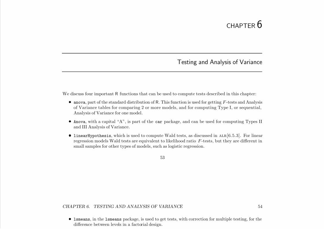
7/18/2019 Computing Primer for Applied Linear Regession by Weisberg
http://slidepdf.com/reader/full/computing-primer-for-applied-linear-regession-by-weisberg 70/153
CHAPTER 6
Testing and Analysis of Variance
We discuss four important R functions that can be used to compute tests described in this chapter:
anova, part of the standard distribution of R. This function is used for getting F -tests and Analysisof Variance tables for comparing 2 or more models, and for computing Type I, or sequential,Analysis of Variance for one model.
Anova, with a capital “A”, is part of the car package, and can be used for computing Types IIand III Analysis of Variance.
linearHypothesis, which is used to compute Wald tests, as discussed in alr[6.5.3]. For linearregression models Wald tests are equivalent to likelihood ratio F -tests, but they are different insmall samples for other types of models, such as logistic regression.
53
CHAPTER 6. TESTING AND ANALYSIS OF VARIANCE 54
lsmeans, in the lsmeans package, is used to get tests, with correction for multiple testing, for thedifference between levels in a factorial design.
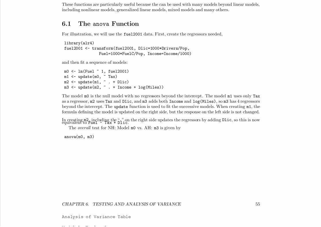
7/18/2019 Computing Primer for Applied Linear Regession by Weisberg
http://slidepdf.com/reader/full/computing-primer-for-applied-linear-regession-by-weisberg 71/153
These functions are particularly useful because the can be used with many models beyond linear models,including nonlinear models, generalized linear models, mixed models and many others.
6.1 The anova Function
For illustration, we will use the fuel2001 data. First, create the regressors needed,
library(alr4)
fuel2001 <- transform(fuel2001, Dlic=1000*Drivers/Pop,
Fuel=1000*FuelC/Pop, Income=Income/1000)
and then fit a sequence of models:
m0 <- lm(Fuel ~ 1, fuel2001)
m1 <- update(m0, ~ Tax)
m2 <- update(m1, ~ . + Dlic)
m3 <- update(m2, ~ . + Income + log(Miles))
The model m0 is the null model with no regressors beyond the intercept. The model m1 uses only Tax
as a regressor, m2 uses Tax and Dlic, and m3 adds both Income and log(Miles), so m3 has 4 regressorsbeyond the intercept. The update function is used to fit the successive models. When creating m1, theformula defining the model is updated on the right side, but the response on the left side is not changed.
In creating m2, including the “.” on the right side updates the regressors by adding Dlic, so this is nowequivalent to Fuel ~ Tax + Dlic.
The overall test for NH: Model m0 vs. AH: m3 is given by
anova(m0, m3)
CHAPTER 6. TESTING AND ANALYSIS OF VARIANCE 55
Analysis of Variance Table
M d l 1 F l 1

7/18/2019 Computing Primer for Applied Linear Regession by Weisberg
http://slidepdf.com/reader/full/computing-primer-for-applied-linear-regession-by-weisberg 72/153
Model 1: Fuel ~ 1
Model 2: Fuel ~ Tax + Dlic + Income + log(Miles)
Res.Df RSS Df Sum of Sq F Pr(>F)
1 50 3956942 46 193700 4 201994 11.992 9.331e-07
The first row of this table is for the fit of m0, fitting only an intercept. The df and RSS for m0 are,respectively, n − 1 and SYY, the total sum of squares. The second row gives the df and RSS for m3, andalso SSreg, the change in df and change in RSS from m0. These differences are required in the numeratorof alr[E6.3]. The F -test shown corresponds exactly to alr[E6.3], in this case with (4, 46) df. ThisF -test is also shown in the summary output for m3:
summary(m3)
Call:
lm(formula = Fuel ~ Tax + Dlic + Income + log(Miles), data = fuel2001)
Residuals:
Min 1Q Median 3Q Max
-163.145 -33.039 5.895 31.989 183.499
Coefficients:
Estimate Std. Error t value Pr(>|t|)
(Intercept) 154.1928 194.9062 0.791 0.432938Tax -4.2280 2.0301 -2.083 0.042873
Dlic 0.4719 0.1285 3.672 0.000626
Income -6.1353 2.1936 -2.797 0.007508
log(Miles) 26.7552 9.3374 2.865 0.006259
CHAPTER 6. TESTING AND ANALYSIS OF VARIANCE 56
Residual standard error: 64.89 on 46 degrees of freedom
Multiple R-squared: 0.5105, Adjusted R-squared: 0.4679
F statistic: 11 99 on 4 and 46 DF p value: 9 331e 07
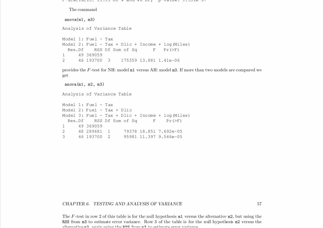
7/18/2019 Computing Primer for Applied Linear Regession by Weisberg
http://slidepdf.com/reader/full/computing-primer-for-applied-linear-regession-by-weisberg 73/153
F-statistic: 11.99 on 4 and 46 DF, p-value: 9.331e-07
The command
anova(m1, m3)
Analysis of Variance Table
Model 1: Fuel ~ Tax
Model 2: Fuel ~ Tax + Dlic + Income + log(Miles)
Res.Df RSS Df Sum of Sq F Pr(>F)
1 49 369059
2 46 193700 3 175359 13.881 1.41e-06
provides the F -test for NH: model m1 versus AH: model m3. If more than two models are compared weget
anova(m1, m2, m3)
Analysis of Variance Table
Model 1: Fuel ~ Tax
Model 2: Fuel ~ Tax + Dlic
Model 3: Fuel ~ Tax + Dlic + Income + log(Miles)
Res.Df RSS Df Sum of Sq F Pr(>F)
1 49 369059
2 48 289681 1 79378 18.851 7.692e-05
3 46 193700 2 95981 11.397 9.546e-05
CHAPTER 6. TESTING AND ANALYSIS OF VARIANCE 57
The F -test in row 2 of this table is for the null hypothesis m1 versus the alternative m2, but using theRSS from m3 to estimate error variance. Row 3 of the table is for the null hypothesis m2 versus thealternative m3 again using the RSS from m3 to estimate error variance

7/18/2019 Computing Primer for Applied Linear Regession by Weisberg
http://slidepdf.com/reader/full/computing-primer-for-applied-linear-regession-by-weisberg 74/153
alternative m3, again using the RSS from m3 to estimate error variance.If anova is used with one argument, we get
anova(m3)
Analysis of Variance Table
Response: Fuel
Df Sum Sq Mean Sq F value Pr(>F)
Tax 1 26635 26635 6.3254 0.0154602
Dlic 1 79378 79378 18.8506 7.692e-05
Income 1 61408 61408 14.5833 0.0003997
log(Miles) 1 34573 34573 8.2104 0.0062592
Residuals 46 193700 4211
This is a sequential or Type I, analysis of variance. The F in the row of Tax tests NH: m1 versusAH: m0. The F in the row for Dlic tests NH: m2 versus AH: m1. Thus each F is a test for addingthe regressor named to a mean function that includes all the regressors listed above it, including anintercept if any. This breakdown is rarely of other than pedagogical interest.
6.2 The Anova Function
The Anova function accepts only one model as an argument:Anova(m3)
Anova Table (Type II tests)
Response: Fuel
CHAPTER 6. TESTING AND ANALYSIS OF VARIANCE 58
Sum Sq Df F value Pr(>F)
Tax 18264 1 4.3373 0.0428733
Dlic 56770 1 13.4819 0.0006256

7/18/2019 Computing Primer for Applied Linear Regession by Weisberg
http://slidepdf.com/reader/full/computing-primer-for-applied-linear-regession-by-weisberg 75/153
Dlic 56770 1 13.4819 0.0006256
Income 32940 1 7.8225 0.0075078
log(Miles) 34573 1 8.2104 0.0062592
Residuals 193700 46These are the Type II tests for each of the coefficients as described in alr[6.2]. Only the test forlog(Miles), the last regressor fit, agrees in Type I and Type II. This function can also be used to getType III tests. For Type I II tests with factors, non-default definition for the contrasts that define thefactors must be used to get the correct answer; see Companion[4.4.4].
6.3 The linearHypothesis Function
A general linear hypothesis alr[6.5.3] can be computed with the linearHypotheis function from thecar package (see also Companion[4.4.5]). To test NH : Lβ = c versus the alternative AH : Lβ = c,the test statistic is alr[E6.21]
F = (L− c)′(LVL′)−1(L − c)
q
Under NH and normality this statistic can be compared with an F (q, n− p′) distribution to get signifi-cance levels. Computing this test requires specifying the matrix L and the vector c. In most instancesc = 0. The general form of calls to the function is
linearHypothesis(model, hypothesis.matrix, rhs)
where model is a fitted model, hypothesis.matrix is either the matrix L are something equivalent,and RHS is c, set to 0 if not specified.
For the UN data,
u1 <- lm(lifeExpF ~ group*log(ppgdp), UN11)
coef(u1)
CHAPTER 6. TESTING AND ANALYSIS OF VARIANCE 59
(Intercept) groupother groupafrica
59.2136614 -11.1731029 -22.9848394
log(ppgdp) groupother:log(ppgdp) groupafrica:log(ppgdp)

7/18/2019 Computing Primer for Applied Linear Regession by Weisberg
http://slidepdf.com/reader/full/computing-primer-for-applied-linear-regession-by-weisberg 76/153
g(ppg p) g p g(ppg p) g p g(ppg p)
2.2425354 0.9294372 1.0949810
We can test for equality of intercepts for levels other and africa using
linearHypothesis(u1, c(0, 1, -1, 0, 0 ,0))
Linear hypothesis test
Hypothesis:
groupother - groupafrica = 0
Model 1: restricted model
Model 2: lifeExpF ~ group * log(ppgdp)
Res.Df RSS Df Sum of Sq F Pr(>F)
1 194 5204.2
2 193 5077.7 1 126.53 4.8094 0.0295
In this case L has only one row. It ignores the first coefficient for the intercept, and then looks at thedifference between the next 2 coefficients, and then ignores the rest. There are several other ways of specifying this, including:
linearHypothesis(u1, "groupother=groupafrica")
linearHypothesis(u1, "groupother-groupafrica")linearHypothesis(u1, "1*groupother - 1*groupafrica = 0")
We can simultaneously test the slope and intercept for other and africa to be equal, with the matrix
L =
( 0 1 −1 0 0 00 0 0 0 1 −1
)
CHAPTER 6. TESTING AND ANALYSIS OF VARIANCE 60
specified as
L <- matrix(c(0, 1, -1, 0, 0, 0,
) )

7/18/2019 Computing Primer for Applied Linear Regession by Weisberg
http://slidepdf.com/reader/full/computing-primer-for-applied-linear-regession-by-weisberg 77/153
0, 0, 0, 0, 1, -1), byrow=TRUE, nrow=2)
linearHypothesis(u1, L)
Linear hypothesis test
Hypothesis:
groupother - groupafrica = 0
groupother:log(ppgdp) - groupafrica:log(ppgdp) = 0
Model 1: restricted model
Model 2: lifeExpF ~ group * log(ppgdp)
Res.Df RSS Df Sum of Sq F Pr(>F)1 195 8081.2
2 193 5077.7 2 3003.5 57.081 < 2.2e-16
The very small p-value suggests that either the slope, intercept, or both is different for the two levels of group. The test for common intercepts with separate slopes was given above with p-value 0.295. Thetest for equal slopes but allowing for separate intercepts uses only the second row of L:
linearHypothesis(u1, L[2, ])
Linear hypothesis test
Hypothesis:
groupother:log(ppgdp) - groupafrica:log(ppgdp) = 0
Model 1: restricted model
CHAPTER 6. TESTING AND ANALYSIS OF VARIANCE 61
Model 2: lifeExpF ~ group * log(ppgdp)
Res.Df RSS Df Sum of Sq F Pr(>F)

7/18/2019 Computing Primer for Applied Linear Regession by Weisberg
http://slidepdf.com/reader/full/computing-primer-for-applied-linear-regession-by-weisberg 78/153
1 194 5079.2
2 193 5077.7 1 1.4597 0.0555 0.814
The help page ?linearHypothesis contains many more examples.
6.4 Comparisons of Means
As an example, consider the wool data treating len, amp and load as factors:
Wool$len <- factor(Wool$len)
Wool$amp <- factor(Wool$amp)
Wool$load <- factor(Wool$load)
m1 <- lm(log(cycles) ~ (len + amp + load)^2, Wool)Anova(m1)
Anova Table (Type II tests)
Response: log(cycles)
Sum Sq Df F value Pr(>F)
len 12.5159 2 301.7441 2.930e-08
amp 7.1674 2 172.7986 2.620e-07
load 2.8019 2 67.5509 9.767e-06len:amp 0.4012 4 4.8357 0.02806
len:load 0.1358 4 1.6364 0.25620
amp:load 0.0146 4 0.1760 0.94456
Residuals 0.1659 8
CHAPTER 6. TESTING AND ANALYSIS OF VARIANCE 62
Because this is a balanced experiment, Type I and Type II analysis of variance are the same so anova
could have been used. Only one of the two-factor interactions appears to be important, so we concentrateon the mean function including only this one interaction,
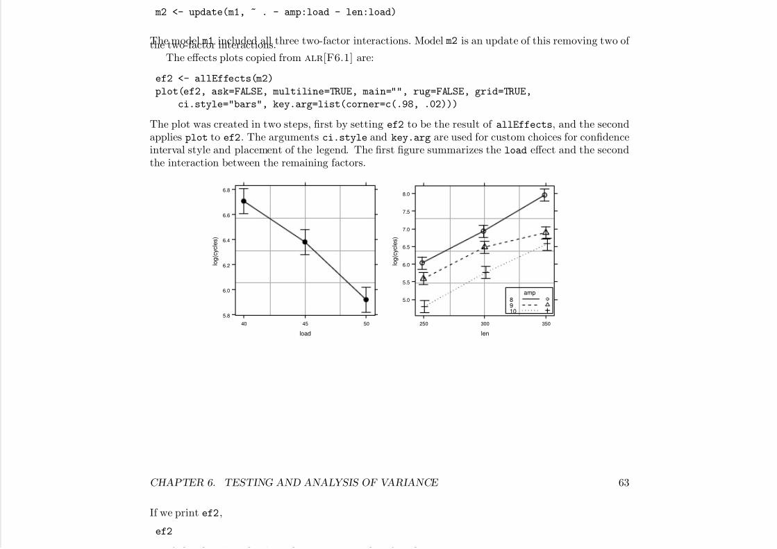
7/18/2019 Computing Primer for Applied Linear Regession by Weisberg
http://slidepdf.com/reader/full/computing-primer-for-applied-linear-regession-by-weisberg 79/153
m2 <- update(m1, ~ . - amp:load - len:load)
The model m1 included all three two-factor interactions. Model m2 is an update of this removing two of the two-factor interactions.The effects plots copied from alr[F6.1] are:
ef2 <- allEffects(m2)
plot(ef2, ask=FALSE, multiline=TRUE, main="", rug=FALSE, grid=TRUE,
ci.style="bars", key.arg=list(corner=c(.98, .02)))
The plot was created in two steps, first by setting ef2 to be the result of allEffects, and the secondapplies plot to ef2. The arguments ci.style and key.arg are used for custom choices for confidenceinterval style and placement of the legend. The first figure summarizes the load effect and the secondthe interaction between the remaining factors.
load
l o g ( c y c l e s )
5.8
6.0
6.2
6.4
6.6
6.8
40 45 50
len
l o g ( c y c l e s )
5.0
5.5
6.0
6.5
7.0
7.5
8.0
250 300 350
amp8910
CHAPTER 6. TESTING AND ANALYSIS OF VARIANCE 63
If we print ef2,
ef2
d l l ( l ) l l d l

7/18/2019 Computing Primer for Applied Linear Regession by Weisberg
http://slidepdf.com/reader/full/computing-primer-for-applied-linear-regession-by-weisberg 80/153
model: log(cycles) ~ len + amp + load + len:amp
load effect
load
40 45 50
6.704924 6.379635 5.919685
len*amp effect
amp
len 8 9 10
250 6.034496 5.584550 4.802098
300 6.931545 6.480485 5.764111
350 7.955145 6.890521 6.569782
These are the adjusted means . The first table for load gives the estimated average response for loadequal to 40, 45 or 50 when the other regressors are fixed at their sample mean values (this default canbe changed by the user). The len*amp table gives the adjusted means for each combination of amp andlen when the regressors that represent load are set equal to their sample mean values. In the case of a balanced experiment like this one, the adjusted means are simply the sample means of the data foreach combination of the focal predictor or predictors.
It is often of interest to compute tests to compare various adjusted means. These are in theorysimply tests concerning linear combinations of coefficients, alr[3.5], but doing the computations can
be complicated in complex models. The lsmeans package (Lenth, 2013) does the required calculations1.
library(lsmeans)
lsmeans(m2, pairwise ~ load)
1lsmeans is not automatically loaded when you load alr4, so the library command shown is required. If you do not
have lsmeans on your system, you can get it with the command install.packages("lsmeans").
CHAPTER 6. TESTING AND ANALYSIS OF VARIANCE 64
$`load lsmeans`
load lsmean SE df lower.CL upper.CL
40 6.704924 0.0468645 16 6.605576 6.804273
45 6 379635 0 0468645 16 6 280286 6 478983

7/18/2019 Computing Primer for Applied Linear Regession by Weisberg
http://slidepdf.com/reader/full/computing-primer-for-applied-linear-regession-by-weisberg 81/153
45 6.379635 0.0468645 16 6.280286 6.478983
50 5.919685 0.0468645 16 5.820337 6.019034
$`load pairwise differences`
estimate SE df t.ratio p.value
40 - 45 0.3252896 0.06627641 16 4.90808 0.00044
40 - 50 0.7852390 0.06627641 16 11.84794 0.00000
45 - 50 0.4599494 0.06627641 16 6.93987 0.00001
p values are adjusted using the tukey method for 3 means
Although the syntax is different, lsmeans and effects do fundamentally the same calculations, witheffects focusing on graphs and lsmeans on tests. The output above gives the estimated means, their
standard errors, and confidence intervals. The pairwise differences are the estimated differences betweenall pairs of means, their standard errors, t-value, and appropriate significance level adjusted for multipletesting. In this example all 3 pairwise comparisons are apparently non-zero with very small p-values.
For the len:amp interaction, we could compare levels for amp for each level of len
lsmeans(m2, pairwise ~ amp|len)[[2]]
estimate SE df t .ratio p.value
8 - 9 | 250 0.4499457 0.1147941 16 3.91959 0.00331
8 - 10 | 250 1.2323981 0.1147941 16 10.73573 0.00000
9 - 10 | 250 0.7824523 0.1147941 16 6.81614 0.000018 - 9 | 300 0.4510601 0.1147941 16 3.92930 0.00324
8 - 10 | 300 1.1674344 0.1147941 16 10.16981 0.00000
9 - 10 | 300 0.7163743 0.1147941 16 6.24051 0.00003
8 - 9 | 350 1.0646238 0.1147941 16 9.27420 0.00000
8 - 10 | 350 1.3853636 0.1147941 16 12.06825 0.00000
CHAPTER 6. TESTING AND ANALYSIS OF VARIANCE 65
9 - 10 | 350 0.3207399 0.1147941 16 2.79404 0.03295
p values are adjusted using the tukey method for 3 means
The [[2]] in the command shortened the output by suppressing the first table of cell means

7/18/2019 Computing Primer for Applied Linear Regession by Weisberg
http://slidepdf.com/reader/full/computing-primer-for-applied-linear-regession-by-weisberg 82/153
The [[2]] in the command shortened the output by suppressing the first table of cell means.Two variations on this:
lsmeans(m2, pairwise ~ len|amp)
compares levels of len for each value of amp, and
lsmeans(m2, pairwise ~ len:amp)
returns all 72 comparisons between the the (len, amp) means.For a more general introduction to the full power of lsmeans, enter the command
vignette("using-lsmeans", package="lsmeans")
into R.
6.5 Power
Suppose we have a regressor X 2 with values 0 and 1, with 0 indicating units that are to be given acontrol treatment and 1 to be given a new treatment, with assignment of units to treatments to be doneat random. In addition, suppose we have p = 5 other regressors, plus an intercept, and n = 20.
A test for a treatment effect is equivalent to testing β 2 = 0 versus β 2 = 0, for which we can use anF -test and reject at level α = 0.05 if the observed value of F exceeds
(crit.val <- qf(1 - .05, 1, 20 - 5 - 1 -1))
[1] 4.667193
CHAPTER 6. TESTING AND ANALYSIS OF VARIANCE 66
Now suppose there is a treatment effect of magnitude β 2/σ = 0.75, where σ is the standard deviationof regression from the fitted model. We measure the size of the the effect in σ units. The probabilitythat the null hypothesis of β 2 = 0 is rejected in this situation is the power of the test, and it dependson the noncentrality parameter λ defined in general at alr[E6 18] and for this particular example just

7/18/2019 Computing Primer for Applied Linear Regession by Weisberg
http://slidepdf.com/reader/full/computing-primer-for-applied-linear-regession-by-weisberg 83/153
on the noncentrality parameter λ defined in general at alr[E6.18], and for this particular example justabove alr[E6.20] by λ = nSD2
2(β 2/σ)2 = 20(.75)2/4 = 2.8125 because SD2
2 = 1/4 for this design. Thepower of the test is
my.power <- function(n=20, lambda=n*.75^2/4, p=5, alpha=0.05){
pf(qf(1-alpha, 1, n-p-1-1),
1, n-p-1-1, lambda, lower.tail=FALSE)
}
my.power()
[1] 0.3425367
We defined my.power as a function with arguments that give the sample size, the noncentrality pa-rameter, the number of additional regressors and the significance level. When executed, my.power callsthe function pf that will return the probability that the value of F exceeds the first argument of thefunction, which is the critical value determined previously. The remaining arguments are the df, thevalue of λ, and lower.tail=FALSE to get the power rather than the probability of Type II error.
The power is disappointing: there is only about a 34% chance of detecting a difference of this size.If we triple the sample size:
my.power(n=60)
[1] 0.813742
we can get up to about 80% power.If the size of the effect of interest is fixed, one can draw a power curve as a function of sample size
to determine the sample size:
CHAPTER 6. TESTING AND ANALYSIS OF VARIANCE 67
plot(1:100, my.power(n=1:100),
xlab="sample size", ylab="power", type="l")
grid(lty=1,col="gray")

7/18/2019 Computing Primer for Applied Linear Regession by Weisberg
http://slidepdf.com/reader/full/computing-primer-for-applied-linear-regession-by-weisberg 84/153
0 20 40 60 80 100
0 . 2
0 . 4
0 . 6
0 . 8
sample size
p o w e r
If sample size is fixed but the effect size is allowed to vary,
plot(seq(0, 2, length=100),
my.power(lambda=20*seq(0,2,length=100)^2/4),
xlab="standardized effect size", ylab="power", type="l")
grid(lty=1,col="gray")
CHAPTER 6. TESTING AND ANALYSIS OF VARIANCE 68
1 . 0

7/18/2019 Computing Primer for Applied Linear Regession by Weisberg
http://slidepdf.com/reader/full/computing-primer-for-applied-linear-regession-by-weisberg 85/153
0.0 0.5 1.0 1.5 2.0
0 . 2
0 . 4
0 . 6
0 . 8
standardized effect size
p o w e r
The function my.power is perfectly general in linear models for computing the power of a test or powercurves. The difficulty is in computing the noncentrality parameter λ, given in general at alr[E6.18] andin special cases at alr[E6.19] and alr[E6.20]. Because using these equations can be difficult, somestatistical packages include power calculators, essentially applications of the my.power for particularsituations. One of these is the power calculator given by Lenth (2006–9), and accessible at http:
//www.stat.uiowa.edu/~rlenth/Power. For example, the “Linear regression” option on Lenth’s powercalculator is for the power of an overall F -test. In the resulting dialog, you can get results similar,but not identical to, the results from my.power by setting No. of predictors = 1, SD of x = .5.Setting Error SD = 1, makes Detectable beta equal to β 2/σ, the effect size. The dialog can be used
to determine any of power, detectable difference, or sample size for given values of the other two.
6.6 Simulating Power
alr[6.4] contains a small simulation to demonstrate the effect of sample size on the significance level
CHAPTER 6. TESTING AND ANALYSIS OF VARIANCE 69
of a test. First, the problem is set up.
MinnLand$fyear <- factor(MinnLand$year)
m1 <- lm(log(acrePrice) ~ fyear + region + year:region, MinnLand)
( )
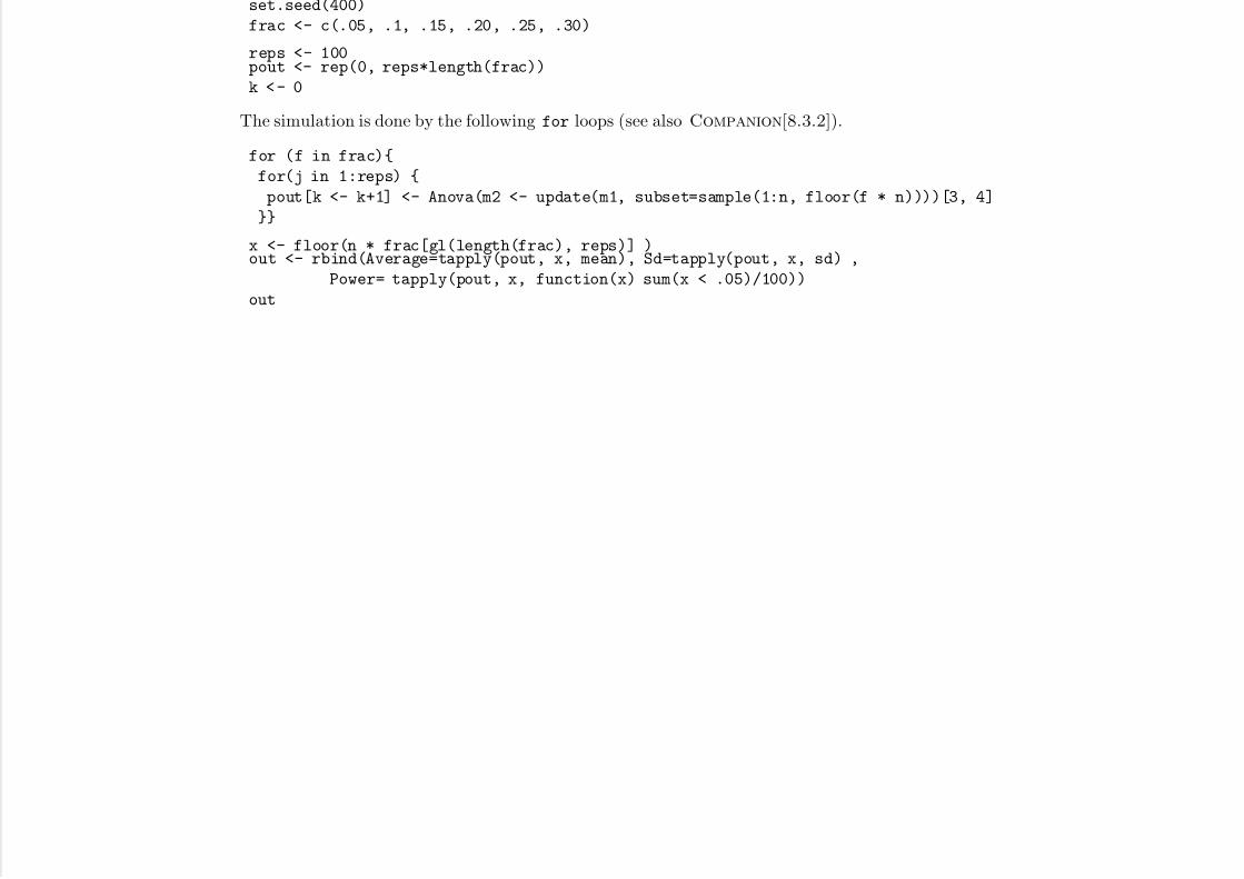
7/18/2019 Computing Primer for Applied Linear Regession by Weisberg
http://slidepdf.com/reader/full/computing-primer-for-applied-linear-regession-by-weisberg 86/153
set.seed(400)
frac <- c(.05, .1, .15, .20, .25, .30)
reps <- 100pout <- rep(0, reps*length(frac))
k < - 0
The simulation is done by the following for loops (see also Companion[8.3.2]).
for (f in frac){
for(j in 1:reps) {
pout[k <- k+1] <- Anova(m2 <- update(m1, subset=sample(1:n, floor(f * n))))[3, 4]
}}
x <- floor(n * frac[gl(length(frac), reps)] )out <- rbind(Average=tapply(pout, x, mean), Sd=tapply(pout, x, sd) ,
Power= tapply(pout, x, function(x) sum(x < .05)/100))
out

7/18/2019 Computing Primer for Applied Linear Regession by Weisberg
http://slidepdf.com/reader/full/computing-primer-for-applied-linear-regession-by-weisberg 87/153
CHAPTER 7
Variances
7.1 Weighted Least Squares
Weighted least squares estimates are most easily obtained using the weights argument for the lmcommand. In the physics data in alr[5.1], the weights are the inverse squares of the variable SD in thedata frame. wls is computed by
m1 <- lm(y ~ x, data=physics, weights=1/SD^2)
summary(m1)
Call:
lm(formula = y ~ x, data = physics, weights = 1/SD^2)
70
CHAPTER 7. VARIANCES 71
Weighted Residuals:
Min 1Q Median 3Q Max
-2.323 -0.884 0.000 1.390 2.335
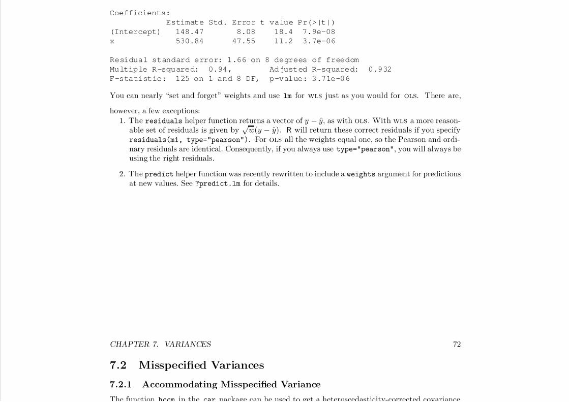
7/18/2019 Computing Primer for Applied Linear Regession by Weisberg
http://slidepdf.com/reader/full/computing-primer-for-applied-linear-regession-by-weisberg 88/153
Coefficients:
Estimate Std. Error t value Pr(>|t|)
(Intercept) 148.47 8.08 18.4 7.9e-08
x 530.84 47.55 11.2 3.7e-06
Residual standard error: 1.66 on 8 degrees of freedom
Multiple R-squared: 0.94, Adjusted R-squared: 0.932
F-statistic: 125 on 1 and 8 DF, p-value: 3.71e-06
You can nearly “set and forget” weights and use lm for wls just as you would for ols. There are,
however, a few exceptions:
1. The residuals helper function returns a vector of y − y, as with ols. With wls a more reason-able set of residuals is given by
√ w(y − y). R will return these correct residuals if you specify
residuals(m1, type="pearson"). For ols all the weights equal one, so the Pearson and ordi-nary residuals are identical. Consequently, if you always use type="pearson", you will always beusing the right residuals.
2. The predict helper function was recently rewritten to include a weights argument for predictionsat new values. See ?predict.lm for details.
CHAPTER 7. VARIANCES 72
7.2 Misspecified Variances
7.2.1 Accommodating Misspecified Variance
The function hccm in the car package can be used to get a heteroscedasticity-corrected covariance
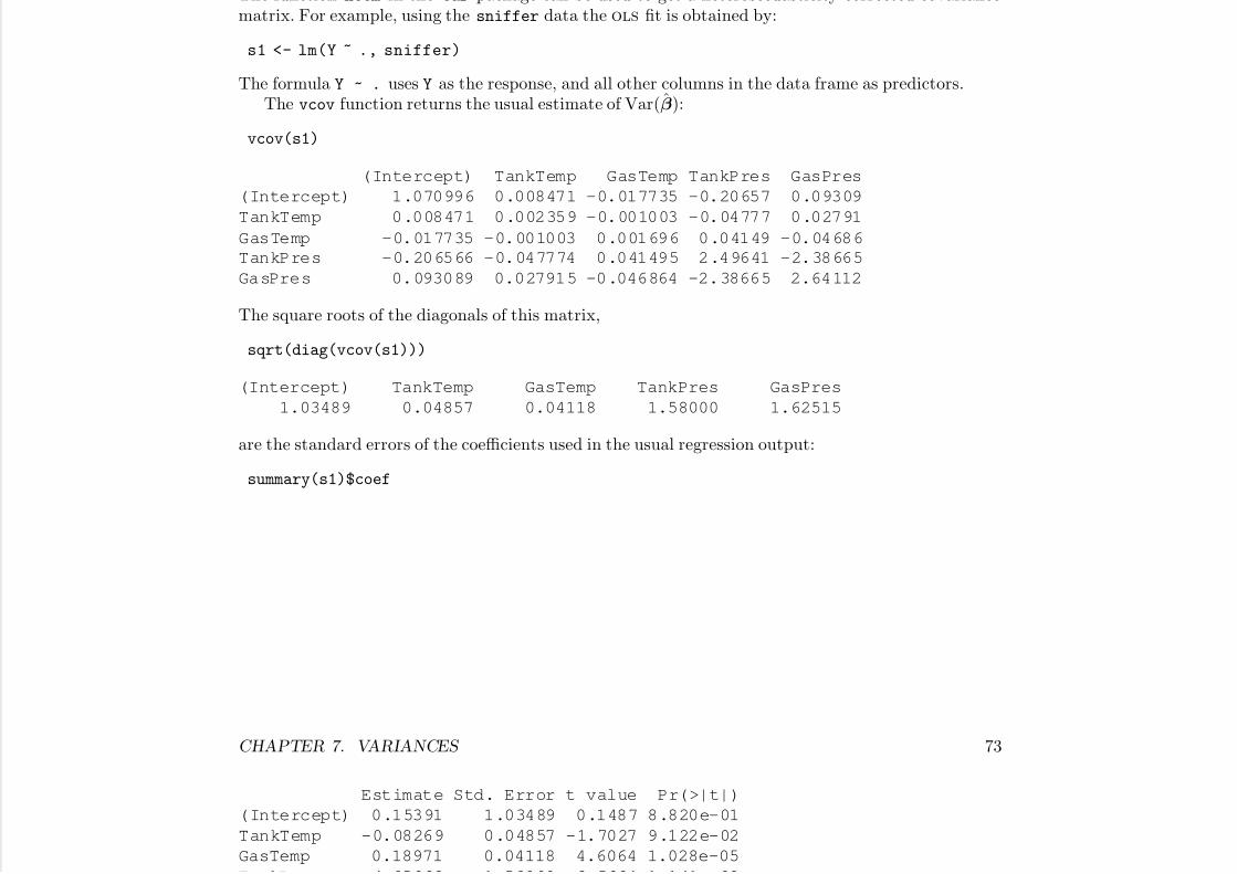
7/18/2019 Computing Primer for Applied Linear Regession by Weisberg
http://slidepdf.com/reader/full/computing-primer-for-applied-linear-regession-by-weisberg 89/153
The function hccm in the car package can be used to get a heteroscedasticity corrected covariancematrix. For example, using the sniffer data the ols fit is obtained by:
s1 <- lm(Y ~ ., sniffer)
The formula Y ~ . uses Y as the response, and all other columns in the data frame as predictors.The vcov function returns the usual estimate of Var(β):
vcov(s1)
(Intercept) TankTemp GasTemp TankPres GasPres
(Intercept) 1.070996 0.008471 -0.017735 -0.20657 0.09309
TankTemp 0.008471 0.002359 -0.001003 -0.04777 0.02791
GasTemp -0.017735 -0.001003 0.001696 0.04149 -0.04686
TankPres -0.206566 -0.047774 0.041495 2.49641 -2.38665
GasPres 0.093089 0.027915 -0.046864 -2.38665 2.64112
The square roots of the diagonals of this matrix,
sqrt(diag(vcov(s1)))
(Intercept) TankTemp GasTemp TankPres GasPres
1.03489 0.04857 0.04118 1.58000 1.62515
are the standard errors of the coefficients used in the usual regression output:
summary(s1)$coef
CHAPTER 7. VARIANCES 73
Estimate Std. Error t value Pr(>|t|)
(Intercept) 0.15391 1.03489 0.1487 8.820e-01
TankTemp -0.08269 0.04857 -1.7027 9.122e-02
GasTemp 0.18971 0.04118 4.6064 1.028e-05
T kP 4 05962 1 58000 2 5694 1 141 02

7/18/2019 Computing Primer for Applied Linear Regession by Weisberg
http://slidepdf.com/reader/full/computing-primer-for-applied-linear-regession-by-weisberg 90/153
TankPres -4.05962 1.58000 -2.5694 1.141e-02
GasPres 9.85744 1.62515 6.0656 1.574e-08
The hc3 estimated is returned by
hccm(s1, type="hc3")
(Intercept) TankTemp GasTemp TankPres GasPres
(Intercept) 1.09693 0.015622 -0.012831 -0.26718 -0.03244
TankTemp 0.01562 0.001975 -0.000641 -0.03916 0.01823
GasTemp -0.01283 -0.000641 0.001142 0.03986 -0.04345
TankPres -0.26718 -0.039156 0.039856 3.89032 -3.86151
GasPres -0.03244 0.018228 -0.043447 -3.86151 4.22652
The function coeftest in the lmtest package1 allows using the output from hccm or any other estimateof Var(β):
library(lmtest)
coeftest(s1, vcov=hccm)
t test of coefficients:
Estimate Std. Error t value Pr(>|t|)(Intercept) 0.1539 1.0473 0.15 0.883
TankTemp -0.0827 0.0444 -1.86 0.065
1lmtest is not automatically loaded when you load alr4, so the library command shown is required. If you do not
have lmtest on your system, you can get it with the command install.packages("lmtest").
CHAPTER 7. VARIANCES 74
GasTemp 0.1897 0.0338 5.61 1.3e-07
TankPres -4.0596 1.9724 -2.06 0.042
GasPres 9.8574 2.0559 4.79 4.7e-06
The R functions linearHypothesis, Anova and deltaMethod in the car package have options to

7/18/2019 Computing Primer for Applied Linear Regession by Weisberg
http://slidepdf.com/reader/full/computing-primer-for-applied-linear-regession-by-weisberg 91/153
yp , p g puse hccm in in place of vcov; see the help pages for these functions.
7.2.2 A Test for Constant Variance
The ncvTest function in the car package can be used to compute the nonconstant variance test (seealso Companion[6.5.2]). To test for nonconstant variance as a function of the mean in the sniffer
data,
ncvTest(s1)
Non-constant Variance Score Test
Variance formula: ~ fitted.values
Chisquare = 4.803 Df = 1 p = 0.02842
To test as a function of TankTemp and GasTemp,
ncvTest(s1, ~ TankTemp + GasTemp)
Non-constant Variance Score Test
Variance formula: ~ TankTemp + GasTemp
Chisquare = 9.836 Df = 2 p = 0.007313
7.3 General Correlation Structures
7.4 Mixed Models
See http://socserv.mcmaster.ca/jfox/Books/Companion-1E/appendix-mixed-models.pdf
CHAPTER 7. VARIANCES 75
The figure alr[F7.4] uses lattice graphics. Here is the R command:
print(xyplot(y ~ loudness, group=subject, data=Stevens, type=c("l", "g", "p"),
xlab="Loudness (db)", ylab="Average log(length)"))
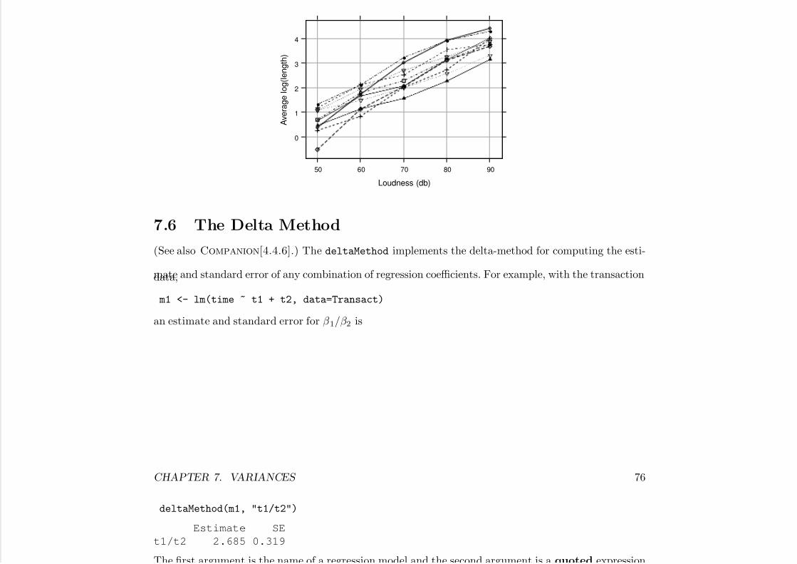
7/18/2019 Computing Primer for Applied Linear Regession by Weisberg
http://slidepdf.com/reader/full/computing-primer-for-applied-linear-regession-by-weisberg 92/153
Loudness (db)
A v e r a g e
l o g ( l e n g t h )
0
1
2
3
4
50 60 70 80 90
7.6 The Delta Method
(See also Companion[4.4.6].) The deltaMethod implements the delta-method for computing the esti-
mate and standard error of any combination of regression coefficients. For example, with the transactiondata,
m1 <- lm(time ~ t1 + t2, data=Transact)
an estimate and standard error for β 1/β 2 is
CHAPTER 7. VARIANCES 76
deltaMethod(m1, "t1/t2")
Estimate SE
t1/t2 2.685 0.319
The first argument is the name of a regression model and the second argument is a quoted expression
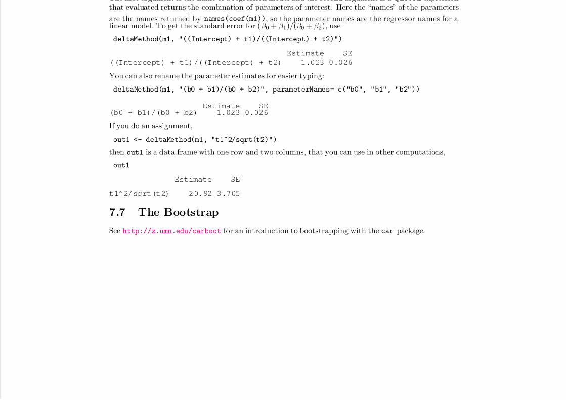
7/18/2019 Computing Primer for Applied Linear Regession by Weisberg
http://slidepdf.com/reader/full/computing-primer-for-applied-linear-regession-by-weisberg 93/153
The first argument is the name of a regression model and the second argument is a quoted expressionthat evaluated returns the combination of parameters of interest. Here the “names” of the parameters
are the names returned by names(coef(m1)), so the parameter names are the regressor names for alinear model. To get the standard error for (β 0 + β 1)/(β 0 + β 2), use
deltaMethod(m1, "((Intercept) + t1)/((Intercept) + t2)")
Estimate SE
((Intercept) + t1)/((Intercept) + t2) 1.023 0.026
You can also rename the parameter estimates for easier typing:
deltaMethod(m1, "(b0 + b1)/(b0 + b2)", parameterNames= c("b0", "b1", "b2"))
Estimate SE(b0 + b1)/(b0 + b2) 1.023 0.026
If you do an assignment,
out1 <- deltaMethod(m1, "t1^2/sqrt(t2)")
then out1 is a data.frame with one row and two columns, that you can use in other computations,
out1
Estimate SE
t1^2/sqrt(t2) 20.92 3.705
7.7 The Bootstrap
See http://z.umn.edu/carboot for an introduction to bootstrapping with the car package.

7/18/2019 Computing Primer for Applied Linear Regession by Weisberg
http://slidepdf.com/reader/full/computing-primer-for-applied-linear-regession-by-weisberg 94/153
CHAPTER 8
Transformations
8.1 Transformation Basics
This chapter uses graphs and smoothers in ways that are uncommon in most most statistical packages,including R (see also Companion[3.4]).
Our solution to this problem is to automate this process with several commands that are included
in the car. These commands become available when you use the command library(alr4) to load thedata files. In the main part of this chapter we show how to use these commands, along with an outlineof what they do. Here is a description of coming attractions.
Transformation families We work with three families of transformations. The basic power family iscomputed with the function basicPower; the Box-Cox power family is computed with bcPower,
77
CHAPTER 8. TRANSFORMATIONS 78
and the Yeo-Johnson family, which can be used if the variable includes non-positive values, iscomputed with yjPower.
Transforming predictors The invTranPlot function provides a graphical method to transform asingle predictor for linearity. The powerTransform function provides a method for transforming
f f

7/18/2019 Computing Primer for Applied Linear Regession by Weisberg
http://slidepdf.com/reader/full/computing-primer-for-applied-linear-regession-by-weisberg 95/153
one or more variables for normality. It also permits conditioning on other, non-transformed
variables.Although these function are adequate for almost all applications, additional function are availablein the car package that are not discussed in alr, including boxTidwell which is essentially anumerical generalization of invTranPlot, and of crPlots for component plus residual plots.
Transforming the response The boxcox command in the MASS package implements the Box-Coxmethod of finding a power transformation. The function boxCox with a capital “C” extends themethod to allow for using the Yeo-Johnson family of transformations, but it is otherwise identicalto boxcox. The powerTransform command provides numeric, rather than graphical, output, forthe same method. The invResPlot is used to transform the response for linearity using a graph.
8.1.1 Power Transformations
8.1.2 Transforming Only the Predictor Variable
The graph in alr[F8.1] uses the scatterplot function in car. Here is the code:
scatterplot(BrainWt ~ BodyWt, brains, id.n=3, boxplots=FALSE, smooth=FALSE, reg=FALSE)
Asian elephant Human African elephant
19 32 33
CHAPTER 8. TRANSFORMATIONS 79
0
5 0 0 0
African elephant
Asian elephant

7/18/2019 Computing Primer for Applied Linear Regession by Weisberg
http://slidepdf.com/reader/full/computing-primer-for-applied-linear-regession-by-weisberg 96/153
0 1000 2000 3000 4000 5000 6000
0
1 0 0 0
2 0 0 0
3 0 0 0
4 0 0 0
BodyWt
B r a i n W t
Human
The scatterplot function is an elaboration of the plot function with many helpful additions to the plotdone either by default or using arguments. This command used the brains data file to plot BrainWt
versus BodyWt. The argument id.n=3 is used in car graphics to identify 3 of the points with labels.With scatterplot points that are “farthest” from the center of the data are labeled. Look at the helppage ?showLabels for complete information. The remaining 3 arguments turn off marginal boxplots, afitted smoother and a fitted ols line, which are included by default with scatterplot.
8.1.3 Transforming One Predictor Variable
The car package includes a function called invTranPlot for drawing the inverse transformation plots
like alr[F8.3].
with(ufcwc, invTranPlot(Dbh, Height))
lambda RSS
1 0.04788 152123
CHAPTER 8. TRANSFORMATIONS 80
2 -1.00000 197352
3 0.00000 152232
4 1.00000 193740

7/18/2019 Computing Primer for Applied Linear Regession by Weisberg
http://slidepdf.com/reader/full/computing-primer-for-applied-linear-regession-by-weisberg 97/153
200 400 600 800 1000
1 0 0
1 5 0
2 0 0
2 5 0
3 0 0
3 5 0
4 0
0
Dbh
H e i g h t
λ^
: 0.05 −1 0 1
The plot command also produces some printed output in the text window, as shown above. This is atable of RSS as a function of the transformation parameter λ, evaluated at λ ∈ (−1, 0, 1) and at thevalue of λ that minimizes RSS, obtained by solving a nonlinear regression problem. In the exampleλ = 0.05 ≈ 0, so the log-transform for Dbh is suggested. See ?invTranPlot for arguments you can useto control this plot.
The function invTranEstimate can be called directly to get the optimal λ without drawing the
graph,
unlist(with(ufcwc, invTranEstimate(Dbh,Height)))
lambda lowerCI upperCI
0.04788 -0.16395 0.25753
CHAPTER 8. TRANSFORMATIONS 81
The minimum value of RSS =152,123. The unlist command made the output prettier.The command bcPower is used by invTranEstimate and by invTranPlot to compute Box-Cox
power transformations. The form of this command is
bcPower(U, lambda, jacobian.adjusted=FALSE)
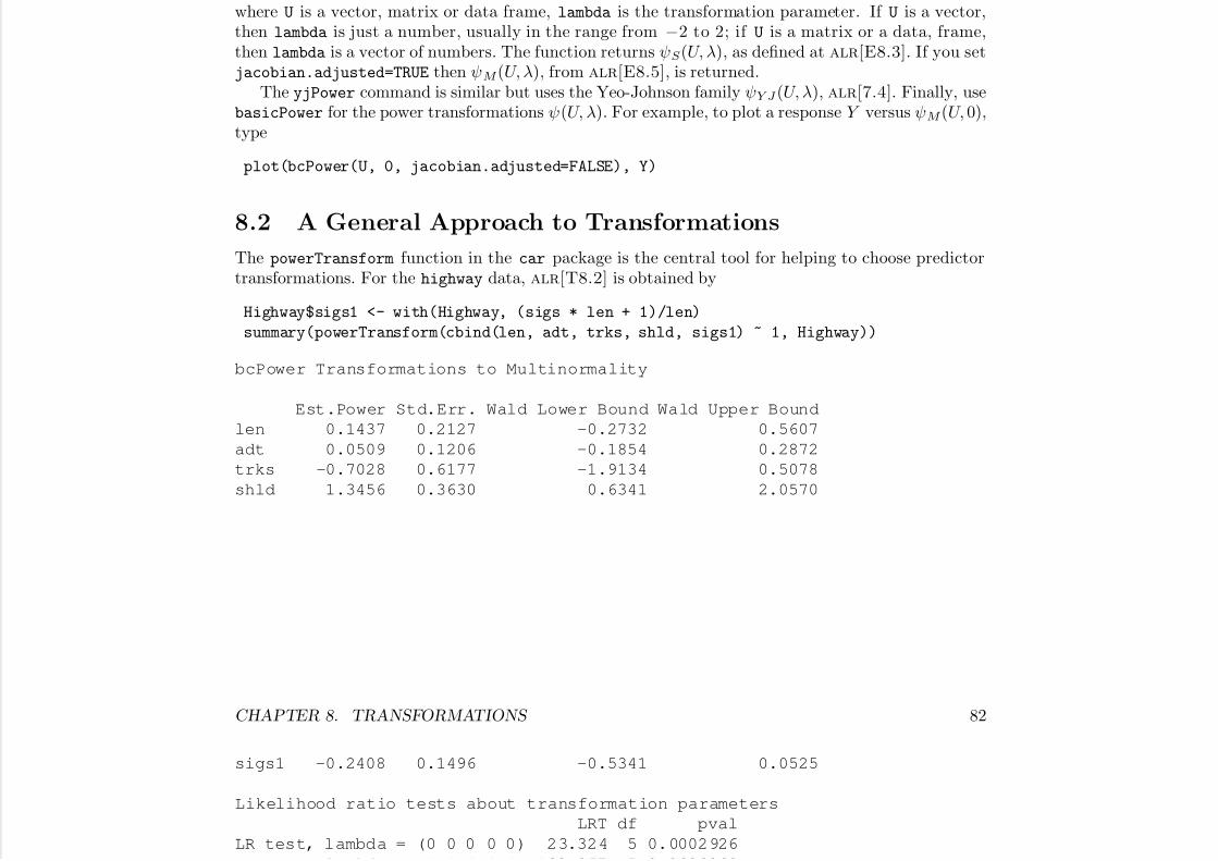
7/18/2019 Computing Primer for Applied Linear Regession by Weisberg
http://slidepdf.com/reader/full/computing-primer-for-applied-linear-regession-by-weisberg 98/153
where U is a vector, matrix or data frame, lambda is the transformation parameter. If U is a vector,then lambda is just a number, usually in the range from −2 to 2; if U is a matrix or a data, frame,then lambda is a vector of numbers. The function returns ψS (U, λ), as defined at alr[E8.3]. If you setjacobian.adjusted=TRUE then ψM (U, λ), from alr[E8.5], is returned.
The yjPower command is similar but uses the Yeo-Johnson family ψY J (U, λ), alr[7.4]. Finally, usebasicPower for the power transformations ψ(U, λ). For example, to plot a response Y versus ψM (U, 0),type
plot(bcPower(U, 0, jacobian.adjusted=FALSE), Y)
8.2 A General Approach to Transformations
The powerTransform function in the car package is the central tool for helping to choose predictortransformations. For the highway data, alr[T8.2] is obtained by
Highway$sigs1 <- with(Highway, (sigs * len + 1)/len)
summary(powerTransform(cbind(len, adt, trks, shld, sigs1) ~ 1, Highway))
bcPower Transformations to Multinormality
Est.Power Std.Err. Wald Lower Bound Wald Upper Bound
len 0.1437 0.2127 -0.2732 0.5607
adt 0.0509 0.1206 -0.1854 0.2872
trks -0.7028 0.6177 -1.9134 0.5078
shld 1.3456 0.3630 0.6341 2.0570
CHAPTER 8. TRANSFORMATIONS 82
sigs1 -0.2408 0.1496 -0.5341 0.0525
Likelihood ratio tests about transformation parameters
LRT df pval
LR test, lambda = (0 0 0 0 0) 23.324 5 0.0002926
l bd (1 1 1 1 1) 132 857 5 0 0000000
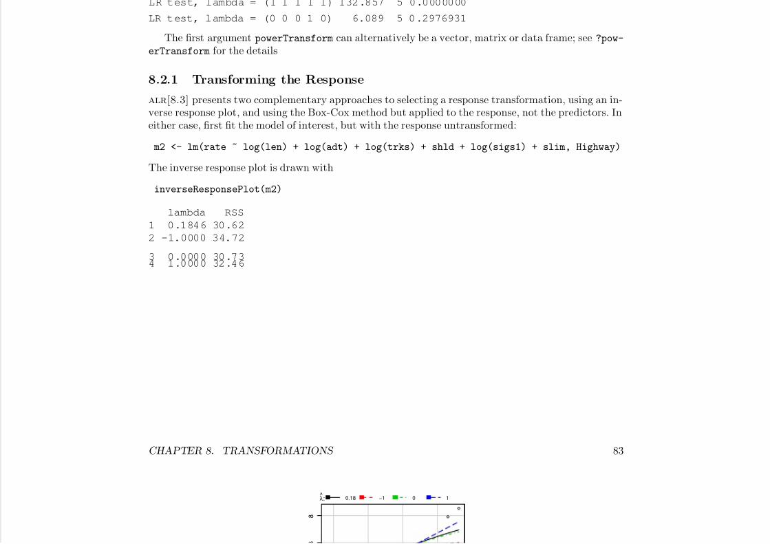
7/18/2019 Computing Primer for Applied Linear Regession by Weisberg
http://slidepdf.com/reader/full/computing-primer-for-applied-linear-regession-by-weisberg 99/153
LR test, lambda = (1 1 1 1 1) 132.857 5 0.0000000
LR t est, l ambda = (0 0 0 1 0) 6.089 5 0 .2976931
The first argument powerTransform can alternatively be a vector, matrix or data frame; see ?pow-
erTransform for the details
8.2.1 Transforming the Response
alr[8.3] presents two complementary approaches to selecting a response transformation, using an in-verse response plot, and using the Box-Cox method but applied to the response, not the predictors. Ineither case, first fit the model of interest, but with the response untransformed:
m2 <- lm(rate ~ log(len) + log(adt) + log(trks) + shld + log(sigs1) + slim, Highway)
The inverse response plot is drawn with
inverseResponsePlot(m2)
lambda RSS
1 0.1846 30.62
2 -1.0000 34.72
3 0.0000 30.734 1.0000 32.46
CHAPTER 8. TRANSFORMATIONS 83
6
8
λ^
: 0.18 −1 0 1

7/18/2019 Computing Primer for Applied Linear Regession by Weisberg
http://slidepdf.com/reader/full/computing-primer-for-applied-linear-regession-by-weisberg 100/153
2 4 6 8
0
2
4
6
rate
y h a t
As with the inverse transformation plot, the values of RSS for the displayed curves are shown in thetext window. In the example the value of λ = 0.18 minimizes RSS, but from alr[F8.7a] there is littleto distinguish using this value of λ from the simpler case of λ = 0, meaning that the fitted curves forthese two values of λ match the data nearly equally well. The log-transform is therefore suggested.
The boxcox function in the MASS package can be used to get alr[F8.7b],
boxCox(m2)
CHAPTER 8. TRANSFORMATIONS 84
7 5
− 7 0
95%

7/18/2019 Computing Primer for Applied Linear Regession by Weisberg
http://slidepdf.com/reader/full/computing-primer-for-applied-linear-regession-by-weisberg 101/153
−2 −1 0 1 2
− 9 0
− 8 5
− 8 0
− 7
λ
l o g − L i k e l i h
o o d
This plot shows the log-likelihood profile function for λ. The estimator maximizes this function1
. If L(λ) is the value of the log-likelihood at λ, then a 95% confidence interval for the λ is the set λ for
which L(λ) ≥ L(λ) − 1.92. You can get the interval printed using
summary(powerTransform(m2))
bcPower Transformation to Normality
Est.Power Std.Err. Wald Lower Bound Wald Upper Bound
Y1 -0.2384 0.2891 -0.805 0.3282
Likelihood ratio tests about transformation parameters
LRT df pval
1boxCox is in the car package. It is based on a very similar function called boxcox in the base R , and adds the ability
to use other families besides the Box-Cox power family.
CHAPTER 8. TRANSFORMATIONS 85
LR test, lambda = (0) 0.6884 1 4.067e-01
LR test, lambda = (1) 18.2451 1 1.942e-05
8.4 Transformations of Nonpositive Variables

7/18/2019 Computing Primer for Applied Linear Regession by Weisberg
http://slidepdf.com/reader/full/computing-primer-for-applied-linear-regession-by-weisberg 102/153
The transformation functions in car
, powerTransform
, inverseResponsePlot
and invTranPlot
, havean argument family, and setting family="yjPower" will use the Yeo-Johnson transformation familyalr[E8.8] in place of the Box-Cox family.
8.5 Additive Models
8.6 Problems

7/18/2019 Computing Primer for Applied Linear Regession by Weisberg
http://slidepdf.com/reader/full/computing-primer-for-applied-linear-regession-by-weisberg 103/153
CHAPTER 9
Regression Diagnostics
R has several functions for working with a fitted model. For example, with the rat data,
m1 <- lm(y ~ BodyWt + LiverWt + Dose, rat)
we can get:
predictions or fitted values using the predict function, for example
predict(m1)
1 2 3 4 5 6 7 8 9 10 11
0.2962 0.3391 0.5359 0.3306 0.2977 0.3129 0.3134 0.3604 0.3177 0.3828 0.3501
86
CHAPTER 9. REGRESSION DIAGNOSTICS 87
12 13 14 15 16 17 18 19
0.3176 0.3082 0.3071 0.3084 0.3388 0.3184 0.3093 0.3253
gives predicted weights for the 19 rats in the data. See ?predict.lm for all the available argumentsfor this helper function.
id l b bt i d i l f ti ( l Com a o [6 1]) O di id l

7/18/2019 Computing Primer for Applied Linear Regession by Weisberg
http://slidepdf.com/reader/full/computing-primer-for-applied-linear-regession-by-weisberg 104/153
residuals can be obtained using several functions (see also Companion[6.1]). Ordinary residuals,given by e = y − y are obtained with residuals(m1). The Pearson residuals, the preferredresiduals in alr, are obtained by residuals(m1, type="pearson"). The standardized residualsalr[E9.18] and Studentized residuals alr[E9.19] are obtained with the rstandard and rstudent
functions, respectively.
leverages defined at alr[E9.12] are returned by the function hatvalues.
Cook’s distance defined in alr[9.5], are returned by the function cooks.distance.
influence The function call influence(m1, do.coef=TRUE)$coefficients returns a matrix whose
i-th row is β (i).
You can use these quantities in graphs or for any other purpose. For example,
press <- residuals(m1) / (1 - hatvalues(m1))
computes and saves the PRESS residuals, alr[P8.4].
par(mfrow=c(1,2))
plot(predict(m1), residuals(m1, type="pearson"))
m2 <- update(m1, ~ . - Dose)
plot(predict(m1), predict(m2))
CHAPTER 9. REGRESSION DIAGNOSTICS 88
0 . 1 0
e a r s o n " )
0 . 3 6

7/18/2019 Computing Primer for Applied Linear Regession by Weisberg
http://slidepdf.com/reader/full/computing-primer-for-applied-linear-regession-by-weisberg 105/153
0.30 0.35 0.40 0.45 0.50
− 0 . 1 0
− 0 . 0 5
0 . 0 0
0 . 0
5
predict(m1)
r e s i d u a l s ( m 1 , t y p e = "
p e
0.30 0.35 0.40 0.45 0.50
0 . 3 0
0 . 3 2
0 . 3 4
predict(m1)
p r e d i c t ( m 2 )
This displays two plots, one of Pearson residuals versus fitted values and the second of fitted valuesfrom two models. Both of these plots could benefit from additions such as point identification, addinga horizontal line at the origin in the right plot, and adding a 45 o line in the second plot.
The car package includes a number of functions that draw graphs related to diagnostic analysis,and 2 of these are particularly useful for the material in alr:
residualPlots This function is for basic residual plotting (see also Companion[6.2.1]). Here are someof the variations:
residualPlot(m1) # Pearson residuals versus fitted values
residualPlots(m1) # array of plots of Pearson residuals versus each regressor
residualPlots(m1, ~ BodyWt, fitted=FALSE) # Pearson residuals versus BodyWt
Plots against splines or polynomials plot versus the predictor that defined the regressors. Plots
CHAPTER 9. REGRESSION DIAGNOSTICS 89
versus factors are boxplots of the Pearson residuals. This function also computes and displays thecurvature tests described in alr[9.2].
As with almost all plots in the car package, you can use point identification:
residualPlots(m1, id.n=2, id.method=list("x", "y"))
T t t t P (>|t|)

7/18/2019 Computing Primer for Applied Linear Regession by Weisberg
http://slidepdf.com/reader/full/computing-primer-for-applied-linear-regession-by-weisberg 106/153
Test stat Pr(>|t|)
BodyWt 0.019 0.985
LiverWt -0.576 0.574
Dose 0.144 0.887
Tukey test 0.932 0.351
1 50 16 0 170 18 0 190 2 00
− 0 . 1
0
0 . 0
0
0 . 0
5
0 . 1
0
BodyWt
P e a r s
o n
r e s i d u a l s
5
17
191
6 7 8 9 10
− 0 . 1
0
0 . 0
0
0 . 0
5
0 . 1
0
LiverWt
P e a r s
o n
r e s i d u a l s
13
8
191
0.75 0.80 0.85 0.90 0.95 1.00
− 0 . 1
0
0 . 0
0
0 . 0
5
0 . 1
0
Dose
P e a
r s o n
r e s i d u a l s
3
5
191
0.30 0.35 0.40 0.45 0.50
− 0 . 1
0
0 . 0
0
0 . 0
5
0 . 1
0
Fitted values
P e a
r s o n
r e s i d u a l s
3
10
191
CHAPTER 9. REGRESSION DIAGNOSTICS 90
In this example setting id.n=2, id.method-list("x", "y") will identify the two most extremepoints in the y , or horizontal direction, and the two most extreme in the x or vertical direction.The latter is required to label to point with the very large fitted value.
As a second example, alr[F9.5] is obtained from
m2 <- lm(fertility ~ log(ppgdp) + pctUrban, UN11)

7/18/2019 Computing Primer for Applied Linear Regession by Weisberg
http://slidepdf.com/reader/full/computing-primer-for-applied-linear-regession-by-weisberg 107/153
residualPlots(m2)
Test stat Pr(>|t|)
log(ppgdp) 5.407 0.000
pctUrban 3.287 0.001
Tukey test 5.420 0.000
CHAPTER 9. REGRESSION DIAGNOSTICS 91
− 1
0
1
2
3
P e a r s o n
r e s i d u a l s
− 1
0
1
2
3
P e a r s o n
r e s i d u a l s

7/18/2019 Computing Primer for Applied Linear Regession by Weisberg
http://slidepdf.com/reader/full/computing-primer-for-applied-linear-regession-by-weisberg 108/153
5 6 7 8 9 10 11
− 2
log(ppgdp)
20 40 60 80 100
− 2
pctUrban
1 2 3 4 5
−
2
− 1
0
1
2
3
Fitted values
P e a r s o n
r e s i d u a l s
In this example all three curvature tests have very small significance levels, leading to the conclu-sion that the model fits poorly.
influenceIndexPlot plots Cook’s distance, Studentized residuals, Bonferroni significance levels totesting each observation in turn to be an outlier, and leverage values, or a subset of these, versusobservation number (see also Companion[6.3.2]).
influenceIndexPlot(m1)
CHAPTER 9. REGRESSION DIAGNOSTICS 92
. 0
0 . 4
0 . 8
C o o k ' s d i s t a n c e
Diagnostic Plots

7/18/2019 Computing Primer for Applied Linear Regession by Weisberg
http://slidepdf.com/reader/full/computing-primer-for-applied-linear-regession-by-weisberg 109/153
0 .
− 1
0
1
2
S t u d e n t i z e d r e s i d u a l
0 . 9
6
0 . 9
8
1 . 0
0
B o n f e r r o n i p − v a l u e
0 . 2
0 . 6
h a t − v a l u e s
5 10 15
Index
9.1 The Residuals
9.1.2 The Hat Matrix
The code for alr[F9.1] is
CHAPTER 9. REGRESSION DIAGNOSTICS 93
n <- dim(UN11)[1]
levs <- pf(99*c(.01, .03, .05, .07), 2, n) - 1/n
with(UN11, dataEllipse(pctUrban, log(ppgdp),
levels=levs - 1/n, xlim=c(-20, 130), ylim=c(3, 14)))

7/18/2019 Computing Primer for Applied Linear Regession by Weisberg
http://slidepdf.com/reader/full/computing-primer-for-applied-linear-regession-by-weisberg 110/153
0 50 100
4
6
8
1 0
1 2
1 4
pctUrban
l o g ( p p g d p )
First n is set to the sample size, and levs are the quantiles of the F (2, n) distribution corresponding
to the values shown. The dataEllipse function in car (see also Companion[4.3.8]) is used to drawthe ellipses. To identify and mark points interactively, the command
with(UN11, identify(pctUrban, log(ppgdp), rownames(UN11)))
can be used. Read ?identify before trying this! (See also Companion[4.3.5].)
CHAPTER 9. REGRESSION DIAGNOSTICS 94
The hat-matrix H is rarely computed in full because it is an n × n matrix that can be very large.Its diagonal entries, the leverages, are computed simply by hatvalues(m1) for a model m1. Should youwish to compute H in full, you can use the following commands. First, suppose that X is an n × pmatrix. Then
decomp <- qr(cbind(rep(1,n),X))
Hat <- qr.Q(decomp) %*% t(qr.Q(decomp))
7/18/2019 Computing Primer for Applied Linear Regession by Weisberg
http://slidepdf.com/reader/full/computing-primer-for-applied-linear-regession-by-weisberg 111/153
q p q p
The use of qr and qr.Q is probably nonintuitive, so here is an explanation. First, append a columnof ones to X for the intercept. Then, compute the QR decomposition, alr[A.9], of the augmentedmatrix. The helper function qr.Q returns Q, and the second command is just alr[EA.27].
9.1.3 Residuals and the Hat Matrix with Weights
As pointed out in alr[8.1.3], the residuals for wls are √
wi × (yi − yi). Whatever computer programyou are using, you need to check to see how residuals are defined.
The correct residuals for wls using R are given by residuals(m1,type="pearson"). These are alsocorrect for ols, and so these should always be used in graphical procedures. The hatvalues functionwill return the correct leverages including the weights.
9.2 Testing for Curvature
The function residualPlots illustrated on page 88 implements the curvature tests described in alr[9.2].
9.3 Nonconstant VarianceThe function ncvTest described in Section 7.2.2 can be used to test for nonconstant variance.
CHAPTER 9. REGRESSION DIAGNOSTICS 95
9.4 Outliers
The function outlierTest returns the values of the outlier test (the Studentized residuals) and thecorresponding Bonferroni-corrected p-values for outlier testing (see also Companion[6.3]).
m2 <- lm(fertility ~ log(ppgdp) + pctUrban, UN11)
outlierTest(m2)
7/18/2019 Computing Primer for Applied Linear Regession by Weisberg
http://slidepdf.com/reader/full/computing-primer-for-applied-linear-regession-by-weisberg 112/153
No Studentized residuals with Bonferonni p < 0.05
Largest |rstudent|:
rstudent unadjusted p-value Bonferonni p
Equatorial Guinea 3.339 0.001007 0.2005
9.5 Influence of Cases
Cook’s distance is computed with the cooks.distance function and displayed in an index plot in the
influenceIndexPlot (e.g., alr[F9.9] function.alr[F9.7] is a complex graph, and we describe how it is obtained. The data in the plot are the
values of β (i), the estimated coefficient estimates computed after deleting the ith case, for 1 = 1, . . . , n.These are obtained in R using
m1 <- lm(log(fertility) ~ log(ppgdp) + lifeExpF, UN11)
betahat.not.i <- influence(m1)$coefficients
The plot was drawn using the pairs function, which has an argument panel that tells pairs what toplot.
panel.fun <- function(x, y, ...){points(x, y, ...)
dataEllipse(x, y, plot.points=FALSE, levels=c(.90))
showLabels(x, y, labels=rownames(UN11),
id.method="mahal", id.n=4)}
CHAPTER 9. REGRESSION DIAGNOSTICS 96
The panel function will use the points function to plot the points, the dataEllipse function from car
to draw the ellipse, and the showLabels function from car to label the extreme points. The plot isfinally drawn with
pairs(betahat.not.i, panel=panel.fun)

7/18/2019 Computing Primer for Applied Linear Regession by Weisberg
http://slidepdf.com/reader/full/computing-primer-for-applied-linear-regession-by-weisberg 113/153
(Intercept)
−0.008 −0.002 0.002
Botswana
Lesotho
South AfricaSwaziland
− 0 . 0
4
0 . 0
0
0 . 0
2
Botswana
Lesotho
South AfricaSwaziland
− 0 . 0
0 8
− 0 . 0
0 2
0 . 0
0 2
Botswana
Lesotho
South Africa
Swaziland
log(ppgdp)
Botswana
Lesotho
South Africa
Swaziland
−0.04 0.00 0.02
Botswana
LesothoSouth Africa
Swaziland
Botswana
LesothoSouth Africa
Swaziland
−0.0005 0.0005 0.0015
− 0 . 0
0 0 5
0 . 0
0 0 5
0 . 0
0 1 5
lifeExpF
CHAPTER 9. REGRESSION DIAGNOSTICS 97
9.6 Normality Assumption
The function qqPlot in the car package can be used to get normal probability plots with the simu-lated envelopes by default, or other quantile-quantile plots for other distributions (see also Compan-ion[6.3.1]). For example, for the UN data regression set up in the last section,
qqPlot(m2, id.n=3)

7/18/2019 Computing Primer for Applied Linear Regession by Weisberg
http://slidepdf.com/reader/full/computing-primer-for-applied-linear-regession-by-weisberg 114/153
Niger Zambia Equatorial Guinea
197 198 199
−3 −2 −1 0 1 2 3
− 2
− 1
0
1
2
3
t Quantiles
S t u d e n t i z e d R e s i d u a l s ( m 2 )
Equatorial GuineaZambiaNiger
The qqPlot function uses Studentized residuals, not Pearson residuals.
CHAPTER 10

7/18/2019 Computing Primer for Applied Linear Regession by Weisberg
http://slidepdf.com/reader/full/computing-primer-for-applied-linear-regession-by-weisberg 115/153
CHAPTER 10
Variable Selection
10.1 Variable Selection and Parameter Assessment
The colinearity diagnostic R2X1,X2
is related to the vif function in car; see Section 4.1.5.
10.2 Variable Selection for Discovery
10.2.1 Information Criteria
The information criteria alr[E10.6–E10.7] depend only on the RSS, p′, and possibly an estimate of σ2, and so if these are needed for a particular model, they can be computed from the usual summaries
98
CHAPTER 10. VARIABLE SELECTION 99
available in a fitted regression model. In addition, the extractAIC can be used to compute aic andbic. For a fitted subset model m0 and a fitted larger model m1, the following commands extract thesequantities:
extractAIC(m0, k=2) # for AIC
extractAIC(m0, k=log(length(residuals(m0)))) # for BIC
10 2 2 St i R i

7/18/2019 Computing Primer for Applied Linear Regession by Weisberg
http://slidepdf.com/reader/full/computing-primer-for-applied-linear-regession-by-weisberg 116/153
10.2.2 Stepwise Regression
The Furnival and Wilson leaps and bounds algorithm mentioned in alr[10.2.2] is implemented in theleaps function in the leaps package. Because of the limitations to this algorithms described in alr,and the relatively difficult to use interface in the implementation in R, most users will not find theall-possible regression approach useful.
The step function in base R can be used for the stepwise approach outlined in alr[10.2.2] (see alsoCompanion[4.5]).
args(step)
function (object, scope, scale = 0, direction = c("both", "backward",
"forward"), trace = 1, keep = NULL, steps = 1000, k = 2,
...)
NULL
The values of these argument depend on whether forward, backward, or stepwise fitting is to be used.As an example, we use the highway data.
Highway$sigs1 <- with(Highway, (sigs * len + 1)/len)
f <- ~ log(len) + shld + log(adt) + log(trks) + lane + slim +lwid +itg + log(sigs1) + acpt + htype
The above commands created the variable sigs1 used in the text. The variable f is a one-sided formulathat will be used below both to update models and as an argument to the step function.
CHAPTER 10. VARIABLE SELECTION 100
Forward Stepwise
Recalling that len is to be included in all models, forward selection is specified by
m0 <- lm(log(rate) ~ log(len), Highway) # the base model
m.forward <- step(m0, scope=f, direction="forward")
Start: AIC=-72 51

7/18/2019 Computing Primer for Applied Linear Regession by Weisberg
http://slidepdf.com/reader/full/computing-primer-for-applied-linear-regession-by-weisberg 117/153
Start: AIC=-72.51log(rate) ~ log(len)
Df Sum of Sq RSS AIC
+ slim 1 2.547 2.94 -94.9
+ acpt 1 2.101 3.38 -89.4
+ shld 1 1.707 3.78 -85.1
+ log(sigs1) 1 0.961 4.52 -78.0
+ htype 3 1.340 4.14 -77.4
+ log(trks) 1 0.728 4.76 -76.1
+ log(adt) 1 0.429 5.06 -73.7
<none> 5.48 -72.5
+ lane 1 0.263 5.22 -72.4
+ itg 1 0.217 5.27 -72.1
+ lwid 1 0.185 5.30 -71.8
Step: AIC=-94.87
log(rate) ~ log(len) + slim
Df Sum of Sq RSS AIC+ acpt 1 0.288 2.65 -96.9
+ log(trks) 1 0.263 2.67 -96.5
<none> 2.94 -94.9
+ log(sigs1) 1 0.147 2.79 -94.9
CHAPTER 10. VARIABLE SELECTION 101
+ htype 3 0.336 2.60 -93.6
+ shld 1 0.033 2.90 -93.3
+ log(adt) 1 0.026 2.91 -93.2
+ lwid 1 0.017 2.92 -93.1
+ lane 1 0.003 2.93 -92.9
+ itg 1 0.003 2.93 -92.9
St AIC 96 9

7/18/2019 Computing Primer for Applied Linear Regession by Weisberg
http://slidepdf.com/reader/full/computing-primer-for-applied-linear-regession-by-weisberg 118/153
Step: AIC=-96.9
log(rate) ~ log(len) + slim + acpt
Df Sum of Sq RSS AIC
+ log(trks) 1 0.1729 2.48 -97.5
<none> 2.65 -96.9
+ log(sigs1) 1 0.1201 2.53 -96.7
+ shld 1 0.0346 2.61 -95.4
+ log(adt) 1 0.0152 2.63 -95.1
+ lane 1 0.0149 2.63 -95.1
+ itg 1 0.0135 2.63 -95.1
+ lwid 1 0.0126 2.64 -95.1
+ htype 3 0.2175 2.43 -94.2
Step: AIC=-97.53
log(rate) ~ log(len) + slim + acpt + log(trks)
Df Sum of Sq RSS AIC
<none> 2.48 -97.5+ shld 1 0.0653 2.41 -96.6
+ log(sigs1) 1 0.0506 2.42 -96.3
+ log(adt) 1 0.0312 2.44 -96.0
+ htype 3 0.2595 2.22 -95.9
CHAPTER 10. VARIABLE SELECTION 102
+ lwid 1 0.0190 2.46 -95.8
+ itg 1 0.0110 2.46 -95.7
+ lane 1 0.0033 2.47 -95.6
The first segment of the above output matches alr[T10.1], except bic was added to the table. Eachstep deletes the regressor or term that will make the greatest decrease the criterion function aic unlessall such deletions increase aic. m.forward will be the model when the stepwise fitting ends (that is,adding another term would increase aic) If trace=0 the output for each step is suppressed
7/18/2019 Computing Primer for Applied Linear Regession by Weisberg
http://slidepdf.com/reader/full/computing-primer-for-applied-linear-regession-by-weisberg 119/153
adding another term would increase aic). If trace=0 the output for each step is suppressed.
Backward Elimination
m1 <- update(m0, f)
m.backward <- step(m1, scope = c(lower = ~ log(len)), direction="backward")
The model m1 includes all the regressors. The lower scope includes log(len), so this must be includedin all models. There is also an upper scope, and since it is not specified it is all the regressors. Had
the lower scope not been specified the default would be lower = ~ 1, the model with no regressors.
Stepwise
R uses direction = "both", the default, for stepwise regression. There are two variations, startingwith the null model,
m.stepup <- step(m0, scope=f)
and starting with all the regressors,
m.stepdown <- step(m1, scope = c(lower = ~ log(len)))
The argument k=2 is used if aic is to be used as the criterion; k=log(n), where n is the sample sizewill use bic. The argument scale is rarely used with linear models.
CHAPTER 10. VARIABLE SELECTION 103
10.2.3 Regularized Methods
The regularized methods briefly described in alr[10.2.3] are the only methods in the first 11 chaptersof alr that use a method other than ols or wls to get estimates. They are designed specifically forthe problem of prediction, and they can be shown to give smaller prediction errors if sample sizes arelarge enough, and the data are like the data that will be observed in the future.
The lasso and elastic net methods can be computed in R using the glmnet.cv function in the glmnet
package (Simon et al., 2011). The alr4 provides a convenience function called Glmnet.cv that allows

7/18/2019 Computing Primer for Applied Linear Regession by Weisberg
http://slidepdf.com/reader/full/computing-primer-for-applied-linear-regession-by-weisberg 120/153
package (Simon et al., 2011). The alr4 provides a convenience function called Glmnet.cv that allowsyou to use the syntax for a formula that is used with lm, and then translate your input into commandsnecessary to run glmnet.cv.
The randomForest package is described by Liaw and Wiener (2002).
10.3 Model Selection for Prediction
10.3.1 Cross Validation
10.4 Problems
CHAPTER 11

7/18/2019 Computing Primer for Applied Linear Regession by Weisberg
http://slidepdf.com/reader/full/computing-primer-for-applied-linear-regession-by-weisberg 121/153
CHAPTER 11
Nonlinear Regression
11.1 Estimation for Nonlinear Mean Functions
11.3 Starting Values
The command nls is used to obtain ols and wls estimates for nonlinear regression models with a
command liken1 <- nls(formula, data, start)
nls differs from lm in a few key respects:
104
CHAPTER 11. NONLINEAR REGRESSION 105
1. The formula argument for defining a model is different. In lm, a typical formula is Y ~ X1 + X2
+ X3 + X4. This formula specifies the names of the response and the regressors, but parametersdo no appear. This causes no particular problem with linear models. If X1 is a variate there is onecorresponding parameter, while if it is a factor, polynomial, interaction or spline there are rulesto determine the parameters from the model specification.
For a nls model, the formula specifies both regressors and parameters. A typical example might
beY ~ th1 + th2 * (1 exp( th3 * x))

7/18/2019 Computing Primer for Applied Linear Regession by Weisberg
http://slidepdf.com/reader/full/computing-primer-for-applied-linear-regession-by-weisberg 122/153
Y ~ th1 + th2 * (1 - exp(-th3 * x))
In this case there are three parameters, th1, th2 and th3, but only one term, x. The right-handside formula should be an expression of parameters, terms, and numbers that can be evaluatedby the computer language C.
2. The data argument provides the name of the data frame with the relevant data, the same as forlm.
3. A named list start of starting values must be specified. This serves the dual purpose of telling the
algorithm where to start, and also to name the parameters. For the example, start=list(th1=620,th2=200, th3=10) indicates that th1, th2 and th3 are parameters, and so by implication theremaining quantity, x, must be a regressor.
4. The data frame must contain the regressors, not predictors that define the regressors. In particular,nls does not permit factors.
5. Most iterative algorithms for nonlinear least squares require computation of derivatives, and manyprograms require the user to provide formulas for the derivatives. This is not the case in nls; allderivatives are computed using numerical differentiation.
Here is the input leading to alr[T11.2]
n1 <- nls(Gain ~ th1 + th2*(1 - exp(-th3 * A)), data=turk0,
start=list(th1=620, th2=200, th3=10))
summary(n1)
CHAPTER 11. NONLINEAR REGRESSION 106
Formula: Gain ~ th1 + th2 * (1 - exp(-th3 * A))
Parameters:
Estimate Std. Error t value Pr(>|t|)
th1 622.96 5.90 105.57 < 2e-16
th2 178.25 11.64 15.32 2.7e-16
th3 7.12 1.21 5.91 1.4e-06

7/18/2019 Computing Primer for Applied Linear Regession by Weisberg
http://slidepdf.com/reader/full/computing-primer-for-applied-linear-regession-by-weisberg 123/153
Residual standard error: 19.7 on 32 degrees of freedom
Number of iterations to convergence: 4
Achieved convergence tolerance: 1.44e-06
We called nls with the required arguments of a formula and starting values. In addition, we specifieda data frame. R has many other arguments to nls, including several that are identical with argumentsof the same name in lm, including subset for selecting cases, weights for using wls, and na.action
for setting the missing value action. A few arguments are used to change the details of the computingalgorithm; see the help page for nls.
Similar to an object created by the lm command, objects created by nls have summary, plot andpredict methods, and these are used in a way that is similar to linear regression models. For example,alr[F11.2] is obtained by
plot(Gain ~ A, turk0, xlab="Amount (percent of diet)", ylab="Weight gain, g")
x <- (0:44)/100
lines(x, predict(n1, data.frame(A=x)))
CHAPTER 11. NONLINEAR REGRESSION 107
7 5 0
8 0 0
a i n ,
g

7/18/2019 Computing Primer for Applied Linear Regession by Weisberg
http://slidepdf.com/reader/full/computing-primer-for-applied-linear-regession-by-weisberg 124/153
0.0 0.1 0.2 0.3 0.4
6 0 0
6 5 0
7 0 0
Amount (percent of diet)
W e i g h t g a
Lack-of-fit testing is possible if there are repeated observations. The idea is to compare the nonlinearfit to the one-way analysis of variance, using the levels of the predictor as a grouping variable:
m1 <- lm(Gain ~ as.factor(A), turk0)
anova(n1,m1)
Analysis of Variance Table
Model 1: Gain ~ th1 + th2 * (1 - exp(-th3 * A))
Model 2: Gain ~ as.factor(A)
Res.Df Res.Sum Sq Df Sum Sq F value Pr(>F)
CHAPTER 11. NONLINEAR REGRESSION 108
1 32 12367
2 29 9824 3 2544 2.5 0.079
The model m1 is a linear model, while n1 is a nonlinear model. Even so, the anova will correctly comparethem, giving the F test for lack of fit.
Factors
Factors and other multi degree of freedom regressors cannot be used directly when using nls For

7/18/2019 Computing Primer for Applied Linear Regession by Weisberg
http://slidepdf.com/reader/full/computing-primer-for-applied-linear-regession-by-weisberg 125/153
Factors and other multi-degree of freedom regressors cannot be used directly when using nls. Forfactors, the corresponding sets of dummy variables must be used in place of the factor. The variable S
in the turkey data frame is an indicator or source of the additive, with levels 1, 2 or 3. We first convertS to a factor and then to a set of 3 dummy indicators for the three levels.
temp <- model.matrix( ~ as.factor(S) -1, turkey)
colnames(temp) <- c("S1", "S2", "S3")
turkey <- cbind(turkey, temp)
The model.matrix command creates the necessary regressors for the one-sided formula specified. Weconverted S to a factor, and removed the intercept with the -1. The column names were corrected, andthen the new columns were added to the data frame.
The code for fitting the four models using wls is given next. The vector m is the number of pens ateach treatment combination, and is the vector of weights for this problem, S is the factor, and Gain isthe response variable.
# fit the models
m4 <- nls( Gain ~ (th1 + th2*(1-exp(-th3*A))),
data=turkey,start=list(th1=620, th2=200, th3=10),
weights=m)# most general
m1 <- nls( Gain ~ S1*(th11 + th21*(1-exp(-th31*A)))+
S2*(th12 + th22*(1-exp(-th32*A)))+
CHAPTER 11. NONLINEAR REGRESSION 109
S3*(th13 + th23*(1-exp(-th33*A))),
data=turkey,
start= list(th11=620, th12=620, th13=620,
th21=200, th22=200, th23=200,
th31=10, th32=10, th33=10),
weights=m)
# common intercept
m2 <- nls(Gain ~ th1 +
( ( ( )))
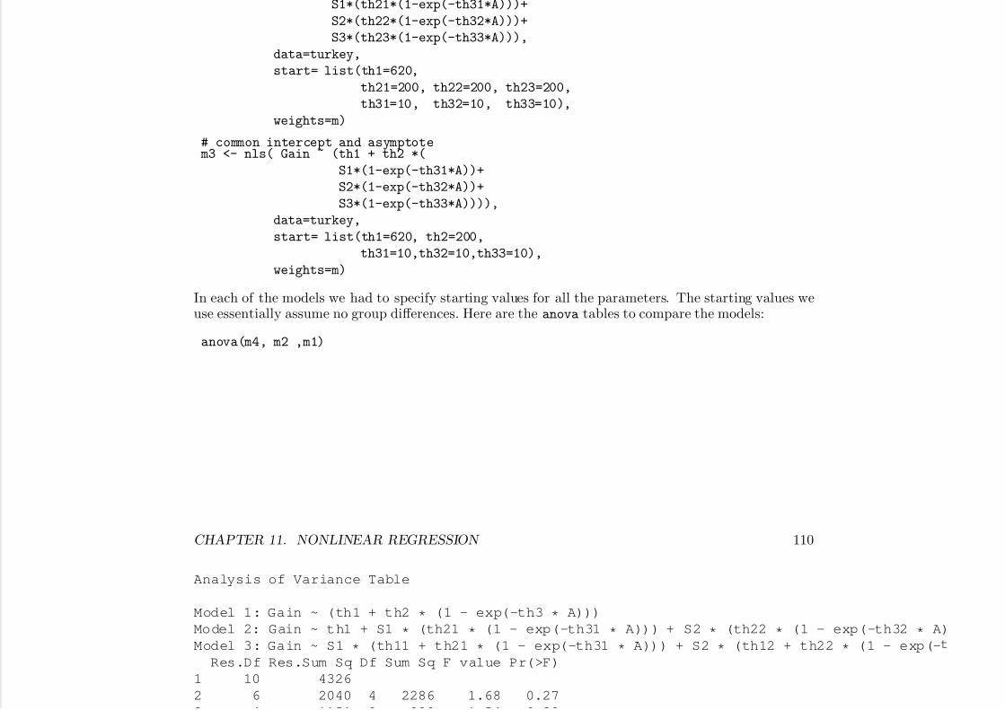
7/18/2019 Computing Primer for Applied Linear Regession by Weisberg
http://slidepdf.com/reader/full/computing-primer-for-applied-linear-regession-by-weisberg 126/153
S1*(th21*(1-exp(-th31*A)))+
S2*(th22*(1-exp(-th32*A)))+
S3*(th23*(1-exp(-th33*A))),
data=turkey,
start= list(th1=620,
th21=200, th22=200, th23=200,
th31=10, th32=10, th33=10),
weights=m)
# common intercept and asymptote m3 <- nls( Gain ~ (th1 + th2 *(
S1*(1-exp(-th31*A))+
S2*(1-exp(-th32*A))+
S3*(1-exp(-th33*A)))),
data=turkey,
start= list(th1=620, th2=200,
th31=10,th32=10,th33=10),
weights=m)
In each of the models we had to specify starting values for all the parameters. The starting values weuse essentially assume no group differences. Here are the anova tables to compare the models:
anova(m4, m2 ,m1)
CHAPTER 11. NONLINEAR REGRESSION 110
Analysis of Variance Table
Model 1: Gain ~ (th1 + th2 * (1 - exp(-th3 * A)))
Model 2: Gain ~ th1 + S1 * (th21 * (1 - exp(-th31 * A))) + S2 * (th22 * (1 - exp(-th32 * A)
Model 3: Gain ~ S1 * (th11 + th21 * (1 - exp(-th31 * A))) + S2 * (th12 + th22 * (1 - exp(-
Res.Df Res.Sum Sq Df Sum Sq F value Pr(>F)
1 10 4326
2 6 2040 4 2286 1.68 0.27
3 4 1151 2 889 1 54 0 32

7/18/2019 Computing Primer for Applied Linear Regession by Weisberg
http://slidepdf.com/reader/full/computing-primer-for-applied-linear-regession-by-weisberg 127/153
3 4 1151 2 889 1.54 0.32
anova(m4, m3, m1)
Analysis of Variance Table
Model 1: Gain ~ (th1 + th2 * (1 - exp(-th3 * A)))
Model 2: Gain ~ (th1 + th2 * (S1 * (1 - exp(-th31 * A)) + S2 * (1 - exp(-th32 * A)) + S3 *Model 3: Gain ~ S1 * (th11 + th21 * (1 - exp(-th31 * A))) + S2 * (th12 + th22 * (1 - exp(-
Res.Df Res.Sum Sq Df Sum Sq F value Pr(>F)
1 10 4326
2 8 2568 2 1758 2.74 0.12
3 4 1151 4 1417 1.23 0.42
A simpler but less general approach to working with a factor uses the nlsList function in the nlme
package.
library(nlme)
n2 <- nlsList(Gain ~ th1 + th2*(1 - exp(-th3 * A))|S, data=turkey,
start=list(th1=620, th2=200, th3=10), pool=TRUE)summary(n2)
Call:
Model: Gain ~ th1 + th2 * (1 - exp(-th3 * A)) | S
CHAPTER 11. NONLINEAR REGRESSION 111
Data: turkey
Coefficients:
th1
Estimate Std. Error t value Pr(>|t|)
1 626.1 6.998 89.47 8.355e-05
2 648.3 14.932 43.42 8.438e-03
3 645.2 14.360 44.93 2.163e-02
th2
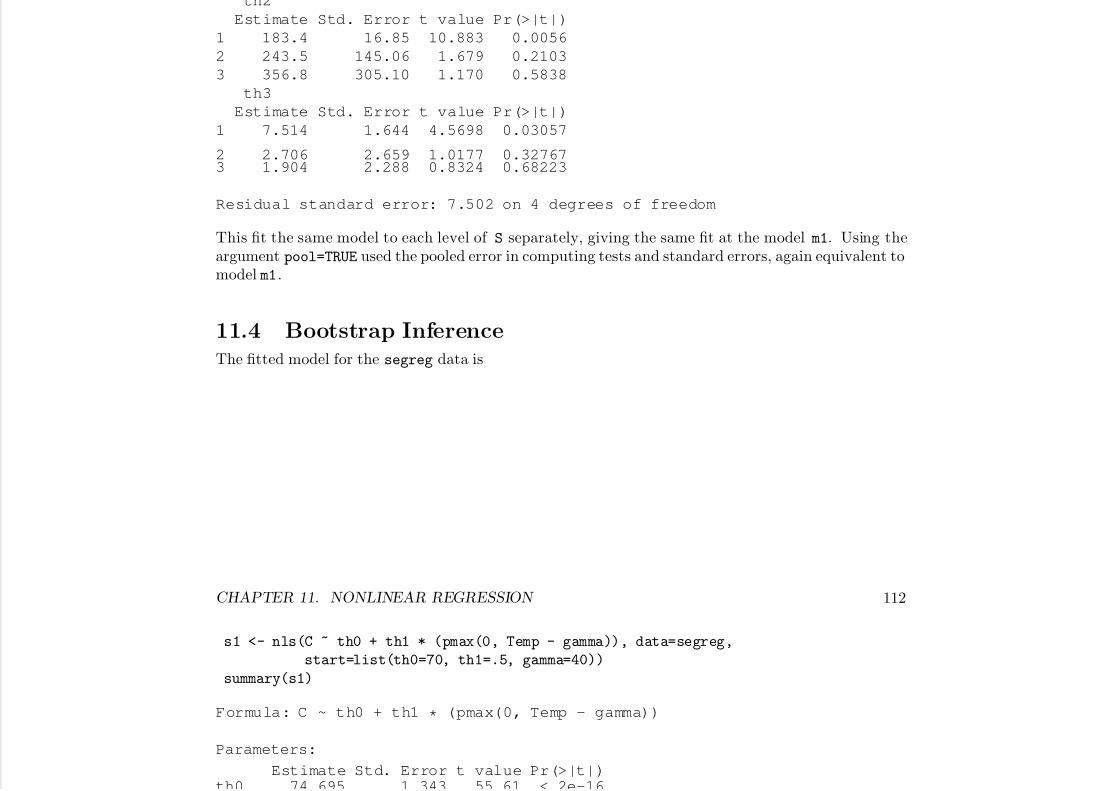
7/18/2019 Computing Primer for Applied Linear Regession by Weisberg
http://slidepdf.com/reader/full/computing-primer-for-applied-linear-regession-by-weisberg 128/153
th2
Estimate Std. Error t value Pr(>|t|)
1 183.4 16.85 10.883 0.0056
2 243.5 145.06 1.679 0.2103
3 356.8 305.10 1.170 0.5838
th3
Estimate Std. Error t value Pr(>|t|)
1 7.514 1.644 4.5698 0.03057
2 2.706 2.659 1.0177 0.327673 1.904 2.288 0.8324 0.68223
Residual standard error: 7.502 on 4 degrees of freedom
This fit the same model to each level of S separately, giving the same fit at the model m1. Using theargument pool=TRUE used the pooled error in computing tests and standard errors, again equivalent tomodel m1.
11.4 Bootstrap Inference
The fitted model for the segreg data is
CHAPTER 11. NONLINEAR REGRESSION 112
s1 <- nls(C ~ th0 + th1 * (pmax(0, Temp - gamma)), data=segreg,
start=list(th0=70, th1=.5, gamma=40))
summary(s1)
Formula: C ~ th0 + th1 * (pmax(0, Temp - gamma))
Parameters:
Estimate Std. Error t value Pr(>|t|)th0 74.695 1.343 55.61 < 2e-16

7/18/2019 Computing Primer for Applied Linear Regession by Weisberg
http://slidepdf.com/reader/full/computing-primer-for-applied-linear-regession-by-weisberg 129/153
th0 74.695 1.343 55.61 < 2e 16
th1 0.567 0.101 5.64 2.1e-06
gamma 41.951 4.658 9.01 9.4e-11
Residual standard error: 5.37 on 36 degrees of freedom
Number of iterations to convergence: 2
Achieved convergence tolerance: 2.6e-08
The pmax function computes element by element maxima for vectors, so pmax(0, Temp - gamma) re-turns a vector of the same length as Temp and equal to Temp if Temp− gamma > 0, and 0 otherwise. Thesummary output matches alr[T11.2].
A bootstrap can be done using the Boot function in the car package. command used for linearmodels. For example, to get the bootstrap leading to alr[F11.5], using R
set.seed(10131985)
s1.boot <- Boot(s1, R=999)
Number of bootstraps was 867 out of 999 attempted
Only 867 of 999 attempted bootstraps converged. For example, of all the cases in the bootstrap hadlarge enough values of Temp, all values of γ smaller than the minimum observed Temp would give thesame fitted model, so γ would not be estimable.
CHAPTER 11. NONLINEAR REGRESSION 113
summary(s1.boot)
R original bootBias bootSE bootMed
th0 867 74.695 0.2325 1.451 74.952
th1 867 0.567 0.0448 0.125 0.582
gamma 867 41.951 1.4724 4.722 42.609
This gives the sample size R, the ols estimates, the difference between the ols estimates and theaverage of the bootstrap estimates called the bootstrap bias), the standard deviation of the bootstraps,

7/18/2019 Computing Primer for Applied Linear Regession by Weisberg
http://slidepdf.com/reader/full/computing-primer-for-applied-linear-regession-by-weisberg 130/153
)which estimates the standard error of the estimates, and the median of the bootstraps. The bootstrapstandard errors are only slightly larger than the standard errors from asymptotic theory.
The bca confidence intervals are
confint(s1.boot)
Bootstrap quantiles, type = bca
2.5 % 97.5 %th0 71.044 77.0674
th1 0.437 0.8338
gamma 36.144 53.0444
and histograms are given by
hist(s1.boot, layout=c(1, 3))
CHAPTER 11. NONLINEAR REGRESSION 114
D e n s i t y
0 . 1
0
0 . 2
0
0 . 3
0
Normal Density
Kernel Densitybca 95% CI
Obs. Value
D e n s i t y
1
2
3
4
5
D e n s i t y
0 . 0
4
0 . 0
8
0 . 1
2

7/18/2019 Computing Primer for Applied Linear Regession by Weisberg
http://slidepdf.com/reader/full/computing-primer-for-applied-linear-regession-by-weisberg 131/153
th0
70 72 74 76 78
0 . 0
0
th1
0.4 0.6 0.8 1.0 1.2 1.4 1.6
0
1
gamma
30 35 40 45 50 55 60
0 . 0
0
CHAPTER 12

7/18/2019 Computing Primer for Applied Linear Regession by Weisberg
http://slidepdf.com/reader/full/computing-primer-for-applied-linear-regession-by-weisberg 132/153
Binomial and Poisson Regression
The glm Function
Binomial and Poisson regression are examples of generalized linear models . These models are fit in R
using the glm function (see also Companion[5]). The usual form of calls to glm is
g1 <- glm(formula, family, data, weights, subset, na.action, start = NULL)
The arguments data, weights, subset and na.action are used in the same way they are used inlm. The family argument is new, and the formula argument is a little different than its use in lm ornls. There are a few other arguments, mostly modifying the computational algorithm, that are rarelyneeded.
115
CHAPTER 12. BINOMIAL AND POISSON REGRESSION 116
Binomial Data
The R command leading to alr[T12.1] is
g1 <- glm(cbind(died, m-died) ~ log(d), family=binomial, data=BlowBS)
The formula argument is cbind(died, m-died) ~ log(d). The response for a binomial response is amatrix with the columns, the first column giving the number of successes, in this case the number of
trees that blew down, and the second column the number of failures, here the number of survivors. Theright-side of the formula is the linear predictor, in this model consisting only of the implied intercept
d ( ) Th ifi bi i l i h f ll i f hi

7/18/2019 Computing Primer for Applied Linear Regession by Weisberg
http://slidepdf.com/reader/full/computing-primer-for-applied-linear-regession-by-weisberg 133/153
and log(d). The family=binomial argument specifies a binomial regression; the full version of thisargument is family=binomial(link="logit") to get logistic regression; see ?family for other standardlink functions (see also Companion[T5.3]). The standard output is:
summary(g1)
Call:
glm(formula = cbind(died, m - died) ~ log(d), family = binomial,
data = BlowBS)
Deviance Residuals:
Min 1Q Median 3Q Max
-1.898 -0.810 0.353 1.135 2.330
Coefficients:
Estimate Std. Error z value Pr(>|z|)
(Intercept) -7.892 0.633 -12.5 <2e-16
log(d) 3.264 0.276 11.8 <2e-16
(Dispersion parameter for binomial family taken to be 1)
Null deviance: 250.856 on 34 degrees of freedom
CHAPTER 12. BINOMIAL AND POISSON REGRESSION 117
Residual deviance: 49.891 on 33 degrees of freedom
AIC: 117.5
Number of Fisher Scoring iterations: 4
This output is very similar to lm output, as explained in alr.The fit summarized in alr[T12.2] uses the data file Blowdown. In this data set the unit of analysis
is a tree, which either survived or died. Fitting with this data file uses binomial regression,
g2 <- glm(y ~ (log(d) + s)^2 binomial Blowdown subset=spp=="balsam fir")

7/18/2019 Computing Primer for Applied Linear Regession by Weisberg
http://slidepdf.com/reader/full/computing-primer-for-applied-linear-regession-by-weisberg 134/153
g2 < glm(y (log(d) + s) 2, binomial, Blowdown, subset=spp== balsam fir )
The response y has values 0 and 11. For binomial regression a matrix with first column the numberof successes and second column the number of failures is not needed. The notation (log(d) + s)^2
expands to log(d) + s + log(d):s, the second-order model.
Poisson Regression
The syntax is similar for Poisson regression models. For the model of alr[T12.5],p1 <- glm(count ~ (type + sex + citizen)^3, poisson, AMSsurvey)
The notation (type + sex + citizen)^3 expands to the second-order model with all main-effects,two-factor and three-factor interactions.
Tests and Deviance
For a glm model, the deviance is returned by the deviance helper function,
c(dev=deviance(g2), df=df.residual(g2))
1The response can also be a factor with two levels. The first level of the factor is considered to be a failure, and the
other level a success.
CHAPTER 12. BINOMIAL AND POISSON REGRESSION 118
dev df
35.75 71.00
The functions Anova, linearHypothesis and deltaMethod work with generalized linear models just asthey do with linear models, returning type II tests by default. For example, for alr[T12.3],
g3 <- glm(y ~ (log(d) + s + spp)^3 , binomial, Blowdown)
Anova(g3)
Analysis of Deviance Table (Type II tests)

7/18/2019 Computing Primer for Applied Linear Regession by Weisberg
http://slidepdf.com/reader/full/computing-primer-for-applied-linear-regession-by-weisberg 135/153
Response: y
LR Chisq Df Pr(>Chisq)
log(d) 228 1 < 2e-16
s 594 1 < 2e-16
spp 510 8 < 2e-16
log(d):s 42 1 1.1e-10
log(d):spp 72 8 2.1e-12
s:spp 36 8 1.4e-05
log(d):s:spp 20 8 0.0088
The tests produced are as discussed in alr[12.3].
12.2 Binomial Regression
alr[F12.2] was drawn with the following commands:
plot( I(died/m) ~ d, BlowBS, xlab="Diameter, cm", ylab="Observed blow down frac.",
cex=.4*sqrt(m), log="x", ylim=c(0,1))
dnew <- seq(3, 40, length=100)
lines(dnew, predict(g1, newdata=data.frame(d=dnew), type="response"), lwd=1.5)
grid(col="gray", lty="solid")
CHAPTER 12. BINOMIAL AND POISSON REGRESSION 119
4
0 . 6
0 . 8
1 . 0
b l o w
d o
w n f r a c .
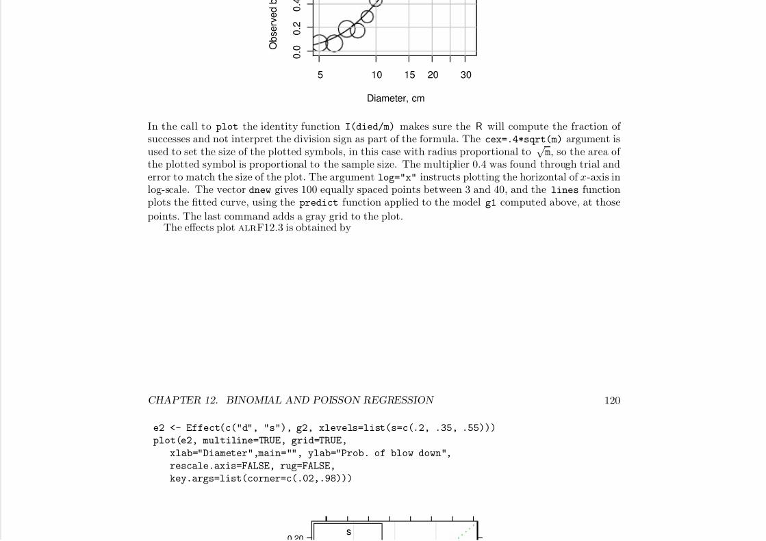
7/18/2019 Computing Primer for Applied Linear Regession by Weisberg
http://slidepdf.com/reader/full/computing-primer-for-applied-linear-regession-by-weisberg 136/153
5 10 15 20 30
0 . 0
0 . 2
0 . 4
Diameter, cm
O b s e r v e d b
In the call to plot the identity function I(died/m) makes sure the R will compute the fraction of successes and not interpret the division sign as part of the formula. The cex=.4*sqrt(m) argument isused to set the size of the plotted symbols, in this case with radius proportional to
√ m, so the area of
the plotted symbol is proportional to the sample size. The multiplier 0.4 was found through trial anderror to match the size of the plot. The argument log="x" instructs plotting the horizontal of x-axis inlog-scale. The vector dnew gives 100 equally spaced points between 3 and 40, and the lines functionplots the fitted curve, using the predict function applied to the model g1 computed above, at those
points. The last command adds a gray grid to the plot.The effects plot alrF12.3 is obtained by
CHAPTER 12. BINOMIAL AND POISSON REGRESSION 120
e2 <- Effect(c("d", "s"), g2, xlevels=list(s=c(.2, .35, .55)))
plot(e2, multiline=TRUE, grid=TRUE,
xlab="Diameter",main="", ylab="Prob. of blow down",
rescale.axis=FALSE, rug=FALSE,
key.args=list(corner=c(.02,.98)))
0 20s
0 2

7/18/2019 Computing Primer for Applied Linear Regession by Weisberg
http://slidepdf.com/reader/full/computing-primer-for-applied-linear-regession-by-weisberg 137/153
Diameter
P r o
b . o f b l o w d
o w n
0.05
0.10
0.15
0.20
6 8 10 12 14 16 18 20
0.2
0.35
0.55
The model g2 was computed above. The call to Effect tells R to compute effects for the highest order
term including c("d", "s"), or for the s:d interaction. Since both of these regressors are continuous,Effect will use its default method for choosing discrete levels of the regressors to plot, but this modifiedby the next xlevels argument for the variable on the horizontal axis.
CHAPTER 12. BINOMIAL AND POISSON REGRESSION 121
The plot function has a method for effects objects. multiline=TRUE will put all the estimated lineson one graph, rather than a separate graph for each line ( multiline=FALSE is the default). The argu-ment rescale.axis controls what is plotted on the vertical axis. If rescale.axis=TRUE, the default,then the vertical axis is labeled with probabilities, but the tick marks are equally spaced in logit scale .If rescale.axis=FALSE, as done in alr[F12.3], then the vertical axis is labeled with probabilities, and
the tick marks are equally spaced in probability scale . The documentation ?plot.eff is unfortunatelycomplex, and the best way to figure out what the arguments do is to try them and see.
The remaining arguments are rug=FALSE, which tells R to not include a so-called rug plot , whichis a small marker in the horizontal axis for each of the observed values of the quantity plotted on thehorizontal axis and key args=list(corner=c( 02 98)) which in this case tells R to put the key

7/18/2019 Computing Primer for Applied Linear Regession by Weisberg
http://slidepdf.com/reader/full/computing-primer-for-applied-linear-regession-by-weisberg 138/153
horizontal axis, and key.args=list(corner=c(.02, .98)), which in this case tells R to put the key2% of the way from the vertical axis and 98% of the way from the horizontal axis.
The effects plot in alr[F12.4] was computed using
e3 <- Effect(c("d", "s","spp"), g3, xlevels=list(s=c(.2, .35, .55 )))
plot(e3, multiline=TRUE, grid=TRUE,
xlab="Diameter",main="", lines=c(1, 3, 2), rotx=45,
ylab="Prob. of blow down", rescale.axis=FALSE, rug=FALSE)
CHAPTER 12. BINOMIAL AND POISSON REGRESSION 122
d
a s p e
n
b a l s a
m f i r
b l a c k
s p r u c e
c e d a
r
j a c k
p i n e
p a p e
r b i r c
h
r e d p i n e
r e d m a p l e
b l a c k
a s h
0 6
0.8
1.0
d
s
0.2
0.35
0.55
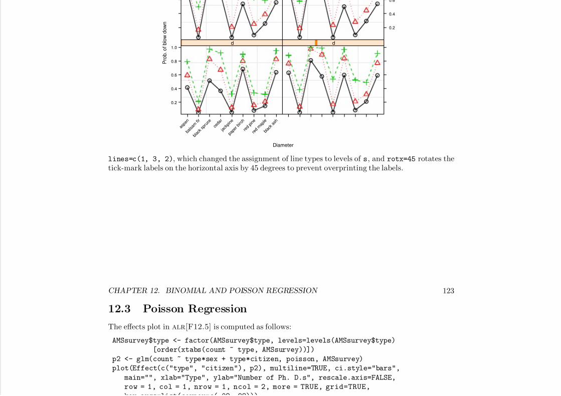
7/18/2019 Computing Primer for Applied Linear Regession by Weisberg
http://slidepdf.com/reader/full/computing-primer-for-applied-linear-regession-by-weisberg 139/153
Diameter
P r o b . o f b l o w d
o w n
0.2
0.4
0.6
0.8
1.0
a s p e
n
b a l s a
m f i r
b l a c k
s p r u c e
c e d a
r
j a c k
p i n e
p a p e
r b i r c
h
r e d p i n e
r e d m a p l e
b l a c k
a s h
d
d
0.2
0.4
0.6
lines=c(1, 3, 2), which changed the assignment of line types to levels of s, and rotx=45 rotates thetick-mark labels on the horizontal axis by 45 degrees to prevent overprinting the labels.
CHAPTER 12. BINOMIAL AND POISSON REGRESSION 123
12.3 Poisson Regression
The effects plot in alr[F12.5] is computed as follows:
AMSsurvey$type <- factor(AMSsurvey$type, levels=levels(AMSsurvey$type)
[order(xtabs(count ~ type, AMSsurvey))])
p2 <- glm(count ~ type*sex + type*citizen, poisson, AMSsurvey)
plot(Effect(c("type", "citizen"), p2), multiline=TRUE, ci.style="bars",
main="", xlab="Type", ylab="Number of Ph. D.s", rescale.axis=FALSE,
row = 1, col = 1, nrow = 1, ncol = 2, more = TRUE, grid=TRUE,
key args=list(corner=c( 02 98)))

7/18/2019 Computing Primer for Applied Linear Regession by Weisberg
http://slidepdf.com/reader/full/computing-primer-for-applied-linear-regession-by-weisberg 140/153
key.args=list(corner=c(.02,.98)))
plot(Effect(c("type", "sex"), p2), multiline=TRUE, ci.style="bars",
main="", xlab="Type", ylab="Number of Ph. D.s", rescale.axis=FALSE,
row = 1, col = 2, nrow = 1, ncol = 2, more = FALSE, grid=TRUE,
key.args=list(corner=c(.02, .98)))
Type
N u m b e r o f P h .
D . s
20
40
60
80
100
120
Va III I(Pr) II I(Pu) IV
citizenNon−USUS
Type
N u m b e r o f P h .
D . s
20
40
60
80
100
120
140
Va III I(Pr) II I(Pu) IV
sexFemaleMale
The first command reordered the levels of type to be ordered according to the number of PhDs in eachof the levels rather than alphabetically. The model p2 fits with only the interactions and main-effects
CHAPTER 12. BINOMIAL AND POISSON REGRESSION 124
of interest. There are several new features to the effects plots themselves. The function Effect is firstcalled to get the highest-order effect based on type and citizen. The ci.style="bars" argumentis used to display uncertainty using bars rather than lines. The set of arguments row = 1, col =
1, nrow = 1, ncol = 2, more = TRUE are used to allow drawing more than one graph in the samewindow. Because plot.eff uses lattice graphics doing this is somewhat obscure. The argumentshere specify that the first plot is in row 1, column 1 of an array with nrows=1 and ncols=2, and themore plots will be drawn. The second plot has more=FALSE.

7/18/2019 Computing Primer for Applied Linear Regession by Weisberg
http://slidepdf.com/reader/full/computing-primer-for-applied-linear-regession-by-weisberg 141/153
APPENDIX A

7/18/2019 Computing Primer for Applied Linear Regession by Weisberg
http://slidepdf.com/reader/full/computing-primer-for-applied-linear-regession-by-weisberg 142/153
Appendix
A.5 Estimating E(Y |X ) Using a Smoother
A bewildering array of options are available for smoothing, both in the base programs, and in packagesavailable from others. In alr, we have almost always used the loess smoother or an older version of it called lowess1. There is no particular reason to prefer this smoother over other smoothers. For thepurposes to which we put smoothers, mainly to help us look at scatterplots, the choice of smoother is
probably not very important.The important problem of choosing a smoothing parameter is generally ignored in alr; one of the
1loess and lowess have different defaults, and so they will give the same answers only if they are set to use the same
tuning parameters.
125
APPENDIX A. APPENDIX 126
nice features of loess is that choosing the smoothing parameter of about 2/3 usually gives good answers.R have several methods for selecting a smoothing parameter; see the references given in alr[A.5], formore information.
The lowess function is used to draw alr[FA.1]
plot(Height ~ Dbh, ufcwc, xlab="Diameter at 137 cm above ground",
ylab="Height, decimeters" )
grid(col="gray", lty="solid")abline(lm(Height ~ Dbh, ufcwc), lty=3, lwd=2)
lines(lowess(ufcwc$Dbh, ufcwc$Height, iter=1, f=.1), lty=4, lwd=2)
li (l ( f $Dbh f $H i ht it 1 f 2/3) lt 1 l d 2)
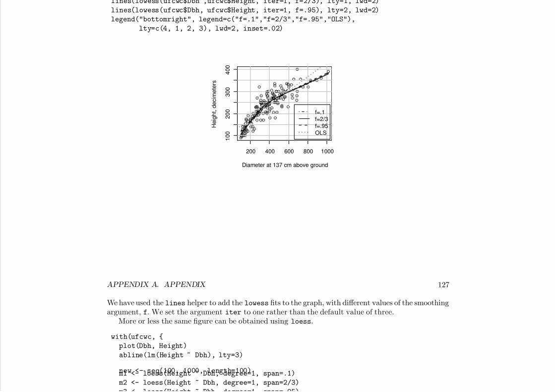
7/18/2019 Computing Primer for Applied Linear Regession by Weisberg
http://slidepdf.com/reader/full/computing-primer-for-applied-linear-regession-by-weisberg 143/153
lines(lowess(ufcwc$Dbh ,ufcwc$Height, iter=1, f=2/3), lty=1, lwd=2)
lines(lowess(ufcwc$Dbh, ufcwc$Height, iter=1, f=.95), lty=2, lwd=2)
legend("bottomright", legend=c("f=.1","f=2/3","f=.95","OLS"),
lty=c(4, 1, 2, 3), lwd=2, inset=.02)
200 400 600 800 1000
1 0 0
2 0 0
3 0 0
4 0 0
Diameter at 137 cm above ground
H e i g h t , d e c i m e t e r s
f=.1f=2/3
f=.95OLS
APPENDIX A. APPENDIX 127
We have used the lines helper to add the lowess fits to the graph, with different values of the smoothingargument, f. We set the argument iter to one rather than the default value of three.
More or less the same figure can be obtained using loess.
with(ufcwc, {
plot(Dbh, Height)
abline(lm(Height ~ Dbh), lty=3)
new <- seq(100, 1000, length=100) m1 <- loess(Height ~ Dbh, degree=1, span=.1)
m2 <- loess(Height ~ Dbh, degree=1, span=2/3)
m3 < loess(Height ~ Dbh degree=1 span= 95)

7/18/2019 Computing Primer for Applied Linear Regession by Weisberg
http://slidepdf.com/reader/full/computing-primer-for-applied-linear-regession-by-weisberg 144/153
m3 <- loess(Height Dbh, degree=1, span=.95)
lines(new, predict(m1, data.frame(Dbh=new)), lty=4, col="cyan")
lines(new, predict(m2, data.frame(Dbh=new)), lty=1, col="red")
lines(new, predict(m3, data.frame(Dbh=new)), lty=2, col="blue")
legend(700, 200, legend=c("f=.1", "f=2/3", "f=.95", "OLS"),
lty=c(4, 1, 2, 3))
})
APPENDIX A. APPENDIX 128
0
2 0 0
3 0 0
4 0 0
H e i g h t , d e c i m e t e r s
f=.1f=2/3f=.95OLS

7/18/2019 Computing Primer for Applied Linear Regession by Weisberg
http://slidepdf.com/reader/full/computing-primer-for-applied-linear-regession-by-weisberg 145/153
200 400 600 800 1000
1 0 0
Diameter at 137 cm above ground
OLS
loess expects a formula. degree=1 uses local linear, rather than quadratic, smoothing, to match
lowess. The span argument is like the f argument for lowess.
A.6 A Brief Introduction to Matrices and Vectors
(See also Companion[8.2].)
A.9 The QR Factorization
R computes the QR factorization using Lapack routines, or the slightly older but equally good Linpackroutines. We illustrate the use of these routines with a very small example.
X <- matrix(c(1, 1, 1, 1, 2, 1, 3, 8, 1, 5, 4, 6), ncol=3,
byrow=FALSE)
APPENDIX A. APPENDIX 129
y <- c(2, 3, -2, 0)
X
[,1] [,2] [,3]
[1,] 1 2 1
[2,] 1 1 5
[3,] 1 3 4
[4,] 1 8 6
y
[1] 2 3 2 0

7/18/2019 Computing Primer for Applied Linear Regession by Weisberg
http://slidepdf.com/reader/full/computing-primer-for-applied-linear-regession-by-weisberg 146/153
[1] 2 3 -2 0
QR <- qr(X)
Here X is a 4 × 3 matrix, and y is a 4 × 1 vector. To use the QR factorization, we start with thecommand qr. This does not find Q or R explicitly but it does return a structure that contains all theinformation needed to compute these quantities, and there are helper functions to return Q and R:
qr.Q(QR)
[,1] [,2] [,3]
[1,] -0.5 -0.27854 0.7755
[2,] -0.5 -0.46424 -0.6215
[3,] -0.5 -0.09285 -0.0605
[4,] -0.5 0.83563 -0.0935
qr.R(QR)
[,1] [,2] [,3]
[1,] -2 -7.000 -8.000
[2,] 0 5.385 2.043
[3,] 0 0.000 -3.135
APPENDIX A. APPENDIX 130
Q is a 4×3 matrix with orthogonal columns, and R is is a 3×3 upper triangular matrix. These matricesare rarely computed in full like this. Rather, other helper functions are used.
In the regression context, there are three helpers that return quantities related to linear regression,using alr[EA.25–EA.27].
qr.coef(QR,y)
[1] 1.7325 -0.3509 0.0614
qr.fitted(QR,y)
[1] 1 0921 1 6886 0 9254 0 7061

7/18/2019 Computing Primer for Applied Linear Regession by Weisberg
http://slidepdf.com/reader/full/computing-primer-for-applied-linear-regession-by-weisberg 147/153
[1] 1.0921 1.6886 0.9254 -0.7061
qr.resid(QR,y)
[1] 0.9079 1.3114 -2.9254 0.7061
qr.coef computes alr[EA.26], qr.fitted computes the fitted values QQ′y, and qr.resid computes
residuals y −QQ′y.The backsolve command is used to solve triangular systems of equations, as described in alr[A.9].The basic linear regression routine lm uses the QR factorization to obtain estimates, standard errors,
residuals and fitted values.
A.10 Spectral Decomposition
The spectral decomposition is computed with the svd function, which stands either for singular valuedecomposition or spectral decomposition. See the R documentation ?svd.
Bibliography

7/18/2019 Computing Primer for Applied Linear Regession by Weisberg
http://slidepdf.com/reader/full/computing-primer-for-applied-linear-regession-by-weisberg 148/153
Fox, J. and Weisberg, S. (2011). An R Companion to Applied Regression . 2nd ed. Sage, ThousandOaks CA. URL http://z.umn.edu/carbook.
Knusel, L. (2005). On the accuracy of statistical distributions in Microsoft Excel 2003. Computational
Statistics and Data Analysis , 48 445–449.
Lenth, R. V. (2006–9). Java applets for power and sample size [computer software]. [Online; accessed15-February-2013], URL http://www.stat.uiowa.edu/~rlenth/Power.
Lenth, R. V. (2013). lsmeans: Least-squares means . R package version 1.06-05, URL http://CRAN.
R-project.org/package=lsmeans.
Liaw, A. and Wiener, M. (2002). Classification and regression by randomforest. R News , 2 18–22.URL http://CRAN.R-project.org/doc/Rnews/.
131
BIBLIOGRAPHY 132
Simon, N., Friedman, J., Hastie, T. and Tibshirani, R. (2011). Regularization paths for cox’sproportional hazards model via coordinate descent. Journal of Statistical Software , 39 1–13. URLhttp://www.jstatsoft.org/v39/i05/.
Weisberg, S. (2014). Applied Linear Regression . 4th ed. Wiley, Hoboken NJ.
Wood, S. (2006). Generalized Additive Models: An Introduction with R, vol. 66. Chapman & Hall/CRC,Boca Raton FL.

7/18/2019 Computing Primer for Applied Linear Regession by Weisberg
http://slidepdf.com/reader/full/computing-primer-for-applied-linear-regession-by-weisberg 149/153
Index

7/18/2019 Computing Primer for Applied Linear Regession by Weisberg
http://slidepdf.com/reader/full/computing-primer-for-applied-linear-regession-by-weisberg 150/153
R functions
%*%, 29abline, 4, 5, 20allEffects, 34, 46, 62Anova, 53, 57, 74, 118anova, 53, 54, 57, 62, 108, 109apply, 28as.matrix, 29avPlots, 24backsolve, 130basicPower, 77bcPower, 77, 81Boot, 112boxCox, 78
boxcox, 78, 83
Boxplot, 43boxTidwell, 78bs, ixc, 13coeftest, 73colMeans, 12confint, 16, 31cooks.distance, 87, 95cor, 16, 28cov, 12, 28cov2cor, 14crossprod, 12crPlots, 78
133
INDEX 134
dataEllipse, 93, 96deltaMethod, 74, 75, 118describe, 28deviance, 117diag, 15dim, xEffect, 34, 38, 45, 120, 124
effect, 34effects, 64extractAIC, 99factor, 41, 43
legend, 5length, 8library, x, 63, 73linearHypotheis, 58linearHypothesis, 53, 58, 74, 118lines, 5, 119, 127lm, 4, 7, 9, 20, 24, 30, 31, 70, 103–106, 117,
130loess, 125–128lowess, 6, 7, 125–128lsmeans, 54, 64, 65

7/18/2019 Computing Primer for Applied Linear Regession by Weisberg
http://slidepdf.com/reader/full/computing-primer-for-applied-linear-regession-by-weisberg 151/153
, ,for, 69formula, 9glm, 115, 117Glmnet.cv, 103glmnet.cv, 103hatvalues, 87, 94hccm, 72–74head, x, 44help, viii, ixI, 26, 46identify, 20influenceIndexPlot, 95install.packages, 63, 73inverseResponsePlot, 85invResPlot, 78
invTranEstimate, 80, 81invTranPlot, 78, 79, 81, 85jpeg, xivleaps, 99
, , , md.pattern, 52 mean, 5, 8 mgcv, 50 model.matrix, 44, 108names, xncvTest, 74, 94nls, 104–106, 108nlsList, 110outlierTest, 95pairs, 7, 8, 95par, 4pdf, xiii, xivpf, 66plot, 1–3, 20, 34, 37, 38, 51, 62, 79, 106,
119, 121
plot.eff, 124pmax, 112points, 96poly, 26, 27, 47, 48
INDEX 135
polym, 49postscript, xivpowerTransform, 78, 81, 82, 85prcomp, 50predict, 17–19, 21, 30, 31, 51, 71, 86, 106,
119print, xi
qF, 15qnorm, 15qqPlot, 97qr, 94, 129
showLabels, 96sigmaHat, 14solve, 29some, 44sqrt, 15step, 99sum, viii
summary, xi, 10, 11, 27, 28, 55, 106, 112svd, 130t, 29tail, 44

7/18/2019 Computing Primer for Applied Linear Regession by Weisberg
http://slidepdf.com/reader/full/computing-primer-for-applied-linear-regession-by-weisberg 152/153
qr.coef, 130qr.fitted, 130qr.Q, 94qr.resid, 130qt, 15read.cvs, xiiiread.table, xi, xiirelevel, 43residualPlots, 20, 94residuals, 20, 31, 71rowMeans, 12rstandard, 87rstudent, 87sample, 22scale, 12, 50
scatterplot, 44, 45, 78, 79scatterplotMatrix, 8sd, 8, 28set.seed, 46
tapply, 4, 5, 8transform, 7, 26unlist, 81update, 54var, 28vcov, 14, 72, 74vif, 36, 98with, 3, 5xyplot, 6yjPower, 78, 81
R packagesalr4, vii, x, xii, 2, 24, 43, 63, 73, 103car, vii–ix, 8, 14, 20, 24, 35, 36, 43, 44, 53,
58, 72, 74, 76–79, 81, 84, 85, 88, 89,93, 96–98, 112
effects, vii, 33, 34, 64foreign, xii, xiiiglmnet, 103lattice, 6, 124
INDEX 136
leaps, 99lmtest, 73lsmeans, 54, 63MASS, 78, 83 mice, 52nlme, 110psych, 28
randomForest, 103splines, ix, 49xlsx, xiii

7/18/2019 Computing Primer for Applied Linear Regession by Weisberg
http://slidepdf.com/reader/full/computing-primer-for-applied-linear-regession-by-weisberg 153/153