arX

iv:q

uant

-ph/

0512

071v

2 1

4 M

ar 2

006

Linear optical quantum computing

Pieter Kok,1, 2, ∗ W.J. Munro,2 Kae Nemoto,3 T.C. Ralph,4 Jonathan P. Dowling,5,6 and G.J. Milburn4

1Department of Materials, Oxford University, Oxford OX1 3PH, UK2Hewlett-Packard Laboratories, Filton Road Stoke Gifford, Bristol BS34 8QZ, UK3National Institute of Informatics, 2-1-2 Hitotsubashi, Chiyoda-ku, Tokyo 101-8430, Japan4Centre for Quantum Computer Technology, University of Queensland, St. Lucia, Queensland 4072, Australia5Hearne Institute for Theoretical Physics, Department of Physics and Astronomy, LSU, Baton Rouge LA, 70803, USA6Institute for Quantum Studies, Department of Physics, Texas A&M University, 77843-4242, USA

(Dated: February 1, 2008)

Linear optics with photon counting is a prominent candidate for practical quantum computing. Theprotocol by Knill, Laflamme, and Milburn [Nature 409, 46 (2001)] explicitly demonstrates that efficientscalable quantum computing with single photons, linear optical elements, and projective measure-ments is possible. Subsequently, several improvements on this protocol have started to bridge the gapbetween theoretical scalability and practical implementation. We review the original theory and itsimprovements, and we give a few examples of experimental two-qubit gates. We discuss the use ofrealistic components, the errors they induce in the computation, and how these errors can be corrected.

PACS numbers: 03.67.Hk, 03.65.Ta, 03.65.Ud

Contents

I. Quantum computing with light 1A. Linear quantum optics 2B. N port interferometers and optical circuits 4C. Qubits in linear optics 4D. Early optical quantum computers and nonlinearities 6

II. A new paradigm for optical quantum computing 8A. Elementary gates 8B. Parity gates and entangled ancillæ 10C. Experimental demonstrations of gates 11D. Characterisation of linear optics gates 13E. General probabilistic nonlinear gates 14F. Scalable optical circuits and quantum teleportation 15

G. The Knill-Laflamme-Milburn protocol 16H. Error correction of the probabilistic gates 18

III. Improvements on the KLM protocol 19A. Cluster states in optical quantum computing 19B. The Yoran-Reznik protocol 21C. The Nielsen protocol 22D. The Browne-Rudolph protocol 22E. Circuit-based optical quantum computing revisited 24

IV. Realistic optical components and their errors 25A. Photon detectors 25B. Photon sources 27C. Circuit errors and quantum memories 32

V. General error correction 33A. Correcting for photon loss 33B. General error correction in LOQC 35

VI. Outlook: beyond linear optics 36

Acknowledgements 37

References 38

∗Electronic address: pieter.kok@materials.ox.ac.uk

I. QUANTUM COMPUTING WITH LIGHT

Quantum computing has attracted much attention overthe last ten to fifteen years, partly because of its promiseof super-fast factoring and its potential for the effi-cient simulation of quantum dynamics. There are manydifferent architectures for quantum computers basedon many different physical systems. These includeatom- and ion-trap quantum computing, superconduct-ing charge and flux qubits, nuclear magnetic resonance,spin- and charge-based quantum dots, nuclear spinquantum computing, and optical quantum computing(for a recent overview see Spiller et al. 2005). All thesesystems have their own advantages in quantum infor-mation processing. However, even though there maynow be a few front-runners, such as ion-trap and su-perconducting quantum computing, no physical imple-mentation seems to have a clear edge over others at thispoint. This is an indication that the technology is still inits infancy. Quantum computing with linear quantumoptics, the subject of this review, has the advantage thatthe smallest unit of quantum information (the photon)is potentially free from decoherence: The quantum in-formation stored in a photon tends to stay there. Thedownside is that photons do not naturally interact witheach other, and in order to apply two-qubit quantumgates such interactions are essential.

Therefore, if we are to construct an optical quantumcomputer, one way or another we have to introduce aneffective interaction between photons. In section I.D,we review the use of so-called large cross-Kerr nonlin-earities to induce a single-photon controlled-NOT op-eration. However, naturally occurring nonlinearities ofthis sort are many orders of magnitude smaller thanwhat is needed for our purposes. An alternative wayto induce an effective interaction between photons isto make projective measurements with photo-detectors.

2

The difficulty with this technique is that such opticalquantum gates are probabilistic: More often than not,the gate fails and destroys the information in the quan-tum computation. This can be circumvented by usingan exponential number of optical modes, but this is bydefinition not scalable (see also section I.D). In 2001,Knill, Laflamme, and Milburn (KLM 2001) constructeda protocol in which probabilistic two-photon gates areteleported into a quantum circuit with high probabil-ity. Subsequent error correction in the quantum circuit isused to bring the error rate down to fault-tolerant levels.We describe the KLM protocol in detail in section II.

Initially, the KLM protocol was designed as a proofthat linear optics and projective measurements allowfor scalable quantum computing in principle. However,it subsequently spurred on new experiments in quan-tum optics, demonstrating the operation of high-fidelityprobabilistic two-photon gates. On the theoretical front,several improvements of the protocol were proposed,leading to ever smaller overhead cost on the computa-tion. A number of these improvements are based oncluster-state quantum computing, or the one-way quan-tum computer. Recently, a circuit-based model wasshown to have similar scaling properties as the best-known cluster state model. In section III, we describethe several improvements to linear optical quantum in-formation processing in considerable detail, and in sec-tion IV, we describe the issues involved in the use ofrealistic components such as photon detectors, photonsources and quantum memories. Given these realisticcomponents, we discuss loss tolerance and general er-ror correction for Linear Optical Quantum Computing(LOQC) in section V.

We will restrict our discussion to the theory of single-photon implementations of quantum information pro-cessors, and we assume some familiarity with the ba-sic concepts of quantum computing. For an introduc-tion to quantum computation and quantum informa-tion, see e.g., Nielsen and Chuang (2000). For a re-view article on optical quantum information process-ing with continuous variables, see Braunstein and VanLoock (2005). In section VI we conclude with anoutlook on other promising optical quantum informa-tion processing techniques, such as photonic band-gapstructures, weak cross-Kerr nonlinearities, and hybridmatter-photon systems. We start our review with a shortintroduction to linear optics, N port optical interferome-ters and circuits, and we define the different versions ofthe optical qubit.

A. Linear quantum optics

The basic building blocks of linear optics are beam split-ters, half- and quarter-wave plates, phase shifters, etc.In this section we will describe these devices mathemat-ically and establish the convention that is used through-out the rest of the paper.

FIG. 1 The beam splitter with transmission amplitude cosθ.

The quantum-mechanical plane-wave expansion ofthe electromagnetic vector potential is usually expressedin terms of the annihilation operators a j(k) and their ad-joints, the creation operators:

Aµ(x, t) =∫

d3k

2ωk∑

j=1,2

ǫµj (k) a j(k) eikx−iωkt + H.c.,

where j indexes the polarisation in the Coulomb gaugeand ǫµj is the corresponding polarisation vector. For the

moment we suppress the polarisation degree of freedomand consider general properties of the creation and anni-hilation operators. They bear their names because theyact in a specific way on the Fock states |n〉:

a|n〉 =√

n|n − 1〉 and a†|n〉 =√

n + 1|n + 1〉 , (1)

where we suppressed the k dependence. It is straight-

forward to show that n(k) ≡ a†(k)a(k) is the numberoperator n|n〉 = n|n〉 for a given mode with momentumk. The canonical commutation relations between a anda† are given by

[a(k), a†(k′)

]= δ(k − k′)

[a(k), a(k′)

]=[

a†(k), a†(k′)]

= 0 . (2)

In the rest of this review, we denote the informationabout the spatial mode, k, by a subscript, since we willnot be concerned with the geometrical details of the in-terferometers we describe, only how the spatial modesare connected. Also, to avoid notational clutter wewill use operator hats only for non-unitary and non-Hermitian operators, as well as cases where omission ofthe hat would lead to confusion.

An important optical component is the single-modephase shift. It changes the phase of the electromagneticfield in a given mode:

a†out = eiφa†inain a†in e−iφa

†inain = eiφ a†in , (3)

with the interaction Hamiltonian Hϕ = φ a†in ain (here,and throughout this review, we use the convention thath = 1, and the time dependence is absorbed in φ).This Hamiltonian is proportional to the number oper-ator, which means that the photon number is conserved.

3

Physically, a phase shifter is a slab of transparent mate-rial with an index of refraction that is different from thatof free space.

Another important component is the beam splitter (seeFig. 1). Physically, it consists of a semi-reflective mir-ror: when light falls on this mirror, part will be reflectedand part will be transmitted. The theory of the losslessbeam splitter is central to LOQC, and was developed byZeilinger (1981) and Fearn and Loudon (1987) . Lossybeam splitters were studied by Barnett et al. (1989) . Thetransmission and reflection properties of general dielec-tric media were studied by Dowling (1998). Let the twoincoming modes on either side of the beam splitter be

denoted by ain and bin, and the outgoing modes by aout

and bout. When we parameterise the probability ampli-tudes of these possibilities as cosθ and sinθ, and therelative phase asϕ, then the beam splitter yields an evo-lution in operator form

a†out = cosθ a†in + ie−iϕ sinθ b†in ,

b†out = ieiϕ sinθ a†in + cosθ b†in , (4)

The reflection and transmission coefficients R and T ofthe beam splitter are R = sin2θ and T = 1 − R = cos2θ.

The relative phase shift ie±iϕ ensures that the transfor-mation is unitary. Typically, we choose either ϕ = 0 orϕ = π/2. Mathematically, the two parameters θ and ϕrepresent the angles of a rotation about two orthogonalaxes in the Poincare sphere. The physical beam splittercan be described by any choice of θ andϕ, provided thecorrect phase shifts are applied to the outgoing modes.

In general the Hamiltonian HBS of the beam splitterevolution in Eq. (4) is given by

HBS = θeiϕ a†inbin +θe−iϕ ainb

†in . (5)

Since the operator HBS commutes with the total numberoperator, [HBS, n] = 0, the photon number is conservedin the lossless beam splitter, as one would expect.

The same mathematical description applies to theevolution due to a polarisation rotation, physically im-plemented by quarter- and half-wave plates. Instead ofhaving two different spatial modes ain and bin, the twoincoming modes have different polarisations. We write

ain → ax and bin → ay for some orthogonal set of coor-dinates x and y (i.e., 〈x|y〉 = 0). The parametersθ andϕare now angles of rotation:

a†x′ = cosθ a†x + ie−iϕ sinθ a†y ,

a†y′ = ieiϕ sinθ a

†x + cosθ a

†y . (6)

This evolution has the same Hamiltonian as the beamsplitter, and it formalises the equivalence between theso-called polarisation and dual-rail logic. These trans-formations are sufficient to implement any photonicsingle-qubit operation (Simon and Mukunda 1990).

The last linear optical element that we highlight hereis the polarising beam splitter (PBS). In circuit diagrams,

FIG. 2 The polarising beam splitter cut to different polarisa-tion bases. (a) The horizontal-vertical basis. (b) The diagonalbasis.

it is usually drawn as a box around a regular beam split-ter (see Fig. 2a). If the PBS is cut to separate horizontaland vertical polarisation, the transformation of the in-coming modes (ain and bin) yields the following outgo-ing modes ((aout and bout):

ain,H → aout,H and ain,V → bout,V

bin,H → bout,H and bin,V → aout,V (7)

We can also cut the PBS to different polarisation direc-tions (e.g., L and R), in which case we make the substi-tution H ↔ L, V ↔ R. Diagrammatically a PBS cut witha different polarisation usually has a circle drawn insidethe box (Fig. 2b).

At this point, we should devote a few words to theterm “linear optics”. Typically this denotes the set of op-tical elements whose interaction Hamiltonian is bilinearin the creation and annihilation operators:

H = ∑jk

A jk a†j ak . (8)

An operator of this form commutes with the total num-ber operator, and has the property that a simple modetransformation of creation operators into a linear combi-nation of other creation operators affects only the matrixA, but does not introduce terms that are quadratic (orhigher) in the creation or annihilation operators. How-ever, from a field-theoretic point of view, the most gen-eral linear Bogoliubov transformation of creation andannihilation operators is given by

a j → ∑k

u jk ak + v jk a†k . (9)

Clearly, when such a transformation is substituted in

Eq. (8) this will give rise to terms such as a j ak and a†j a†k,

i.e., squeezing. The number of photons is not conservedin such a process. For the purpose of this review, we ex-clude squeezing as a resource other than as a method forgenerating single photons.

With the linear optical elements introduced in this sec-tion we can build large optical networks. In particular,

4

FIG. 3 Decomposing an N port unitary U(N) into SU(2)group elements, i.e., beam splitters and phase shifters. More-over, this is an efficient process: the maximum number ofbeam splitters needed is N(N − 1)/2.

we can make computational circuits by using knownstates as the input and measuring the output states.Next we will study these optical circuits in more detail.

B. N port interferometers and optical circuits

An optical circuit can be thought of as a black box withincoming and outgoing modes of the electromagneticfield. The black box transforms a state of the incomingmodes into a different state of the outgoing modes. Themodes might be mixed by beam splitters, or they maypick up a relative phase shift or polarisation rotation.These operations all belong to a class of optical compo-nents that preserve the photon number, as described inthe previous section. In addition, the box may includemeasurement devices, the outcomes of which may mod-ify optical components on the remaining modes. Thisis called feed-forward detection, and it is an importanttechnique that can increase the efficiency of a device(Lapaire et al. 2003; Clausen et al. 2003).

Optical circuits can also be thought of as a general uni-tary transformation on N modes, followed by the de-tection of a subset of these modes (followed by unitarytransformation on the remaining modes, detection, andso on). The interferometric part of this circuit is alsocalled an N port interferometer. N ports yield a uni-tary transformation U of the spatial field modes ak, withj, k ∈ 1, . . . , N:

bk →N

∑j=1

U jka j and b†k →

N

∑j=1

U∗jka

†j , (10)

where the incoming modes of the N port are denoted bya j and the outgoing modes by b j. The explicit form of Uis given by the repeated application of transformationssuch as given in Eqs. (3), (4), and (6).

The two-mode operators L+ = a† b, L− = ab†, and

L0 = (a† a − b† b)/2 form an su(2) Lie algebra:

[L0 , L±] = ±L± and [L+, L−] = 2L0 . (11)

This means that any two-mode interferometer exhibits

U(2) symmetry1. In general, an N port interferometercan be described by a transformation from the groupU(N). Reck et al. (1994) demonstrated that the converseis also true, i.e., that any unitary transformation of Noptical modes can be implemented efficiently with an Nport interferometer . They showed how a general U(N)element can be broken down into SU(2) elements, forwhich we have a complete physical representation interms of beam splitters and phase shifters (see Fig. 3).The primitive element is a matrix Tpq defined on themodes p and q, which corresponds to a beam splitterand phase shifts. Implicit in this notation is the iden-tity operator on the rest of the optical modes, such thatTpq ≡ Tpq ⊗ 11rest. We then have

U(N) · TN,N−1 · · · TN,1 = U(N − 1) ⊕ eiφ , (12)

whereφ is a single-mode phase. Concatenating this pro-cedure leads to a full decomposition of U(N) into T ele-ments, which in turn are part of SU(2). The maximumnumber of beam splitter elements T that are needed isN(N − 1)/2. This procedure is thus manifestly scalable.

Subsequently, it was shown by Torma et al. (1995,1996) and Jex et al. (1995) how one can construct multi-mode Hamiltonians that generate these unitary mode-transformations, and a three-path Mach-Zehnder inter-ferometer was demonstrated experimentally by Weihset al. (1996). A good introduction to linear optical net-works is given by Leonhardt (2003) and a determina-tion of effective Hamiltonians is given by Leonhardt andNeumaier (2004). For a treatment of optical networks interms of their permanents, see Scheel (2004). Optical cir-cuits in a (general) relativistic setting are described byKok and Braunstein (2006).

C. Qubits in linear optics

Formally, a qubit is a quantum system with an SU(2)symmetry. We saw above that two optical modes forma natural implementation of this symmetry. In gen-eral, two modes with fixed total photon number n fur-nish natural irreducible representations of this groupwith the dimension of the representation given by n + 1(Biedenharn and Louck 1981). It is at this point notspecified whether we should use spatial or polarisationmodes. In linear optical quantum computing, the qubit

1 Two remarks: Algebras are typically denoted in lower-case, whilethe group itself is denoted in upper-case. Secondly, single-modephase shifts break the “special” symmetry (det U = 1), which iswhy an interferometer is described by U(N), rather than SU(N).

5

of choice is usually taken to be a single photon that hasthe choice of two different modes |0〉L = |1〉 ⊗ |0〉 ≡|1, 0〉 and |1〉L = |0〉 ⊗ |1〉 ≡ |0, 1〉. This is calleda dual-rail qubit. When the two modes represent theinternal polarisation degree of freedom of the photon(|0〉L = |H〉 and |1〉L = |V〉), we speak of a polari-sation qubit. In this review we will reserve the term“dual rail” for a qubit with two spatial modes. As weshowed earlier, these two representations are mathe-matically equivalent, and we can physically switch be-tween them using polarisation beam splitters. In addi-tion, some practical applications (typically involving adephasing channel such as a fibre) may call for so-calledtime-bin qubits, in which the two computational qubitvalues are “early” and “late” arrival times in a detec-tor. However, this degree of freedom does not exhibita natural internal SU(2) symmetry: Arbitrary single-qubit operations are very difficult to implement. In thisreview we will be concerned mainly with polarisationand dual-rail qubits.

In order to build a quantum computer, we need bothsingle-qubit operations as well as two-qubit operations.Single-qubit operations are generated by the Pauli op-erators σx, σy, and σz, in the sense that the operatorexp(iθσ j) is a rotation about the j-axis in the Blochsphere with angle θ. As we have seen, these operationscan be implemented with phase shifters, beam splitters,and polarisation rotations on polarisation and dual-railqubits. In this review, we will use the convention thatσx, σy, and σz denote physical processes, while we useX, Y, and Z for the corresponding logical operations onthe qubit. These two representations become inequiva-lent when we deal with logical qubits that are encodedin multiple physical qubits.

Whereas single-qubit operations are straightforwardin the polarisation and dual-rail representation, the two-qubit gates are more problematic. Consider, for exam-ple, the transformation from a state in the computationalbasis to a maximally entangled Bell state:

|H, H〉ab → 1√2

(|H, V〉cd + |V, H〉cd) . (13)

This is the type of transformation that requires a two-qubit gate. In terms of the creation operators (and ig-noring normalisation), the linear optical circuit that issupposed to create Bell states out of computational ba-sis states is described by a Bogoliubov transformation ofboth creation operators

a†H b†H →(

∑k=H,V

αkc†k +βk d†k

)(

∑k=H,V

γk c†k + δkd†k

)

6= c†H d†V + c†V d†H . (14)

It is immediately clear that the right-hand sides in bothlines cannot be made the same for any choice of αk, βk,γk, and δk: The top line is a separable expression in thecreation operators, while the bottom line is an entangled

expression in the creation operators. Therefore, linearoptics alone cannot create maximal polarisation entan-glement from single polarised photons in a determinis-tic manner (Kok and Braunstein 2000a). Entanglementthat is generated by changing the definition of our sub-systems in terms of the global field modes is inequiv-alent to the entanglement that is generated by apply-ing true two-qubit gates to single-photon polarisation ordual-rail qubits.

Note also that if we choose our representation ofthe qubit differently, we can implement a two-qubittransformation. Consider the single-rail qubit encoding|0〉L = |0〉 and |1〉L = |1〉. That is, the qubit is givenby the vacuum and the single-photon state. We canthen implement the following (unnormalised) transfor-mation deterministically:

|1, 0〉 → |1, 0〉+ |0, 1〉 . (15)

This is a 50:50 beam splitter transformation. However,in this representation the single-qubit operations cannotbe implemented deterministically with linear optical el-ements, since these transformations do not preserve thephoton number (Paris 2000). This implies that we can-not implement single-qubit and two-qubit gates deter-ministically for the same physical representation. Forlinear optical quantum computing, we typically needthe ability to (dis-) entangle field modes. We thereforehave to add a non-linear component to our scheme. Twopossible approaches are the use of Kerr nonlinearities,which we briefly review in the next section, and the useof projective measurements. In the rest of this review, weconcentrate mainly on linear optical quantum comput-ing with projective measurements, based on the workby Knill, Laflamme, and Milburn.

Finally, in order to make a quantum computer withlight that can outperform any classical computer, weneed to understand more about the criteria that makequantum computers “quantum”. For example, somesimple schemes in quantum communication requireonly superpositions of quantum states to distinguishthem from their corresponding classical ones. However,we know that this is not sufficient for general computa-tional tasks.

First, we give two definitions. The Pauli groupP is the set of Pauli operators with coefficients±1, ±i. For instance, the Pauli group for one qubitis 11, ±X, ±Y, ±Z, ±i11 ± iX, ±iY, ±iZ, where 11 is theidentity matrix. The Pauli group for n qubits consistsof elements that are products of n Pauli operators, in-cluding the identity. In addition, we define the Cliffordgroup C of transformations that leave the Pauli group in-variant. In other words, for any element of the Cliffordgroup c and any element of the Pauli group p, we have

cpc† = p′ with p′ ∈ P . (16)

Prominent members of the Clifford group are theHadamard transformation, phase transformations, and

6

FIG. 4 Linear optical quantum computing simulation accord-ing to Cerf, Adami, and Kwiat. (a) Hadamard gate. (b) CNOTgate. The four two-qubit degrees of freedom are carried bywhich-path and polarization information. The broken line in-dicates that there is no interaction between the crossing modes.

the controlled-not (CNOT)2 Note that the Pauli group isa subgroup of the Clifford group.

The Gottesman-Knill theorem (1999) states that anyquantum algorithm that initiates in the computationalbasis and employs only transformations (gates) from thethe Clifford group, along with projective measurementsin the computational basis, can be efficiently simulatedon a classical computer. This means there is no computa-tional advantage in restricting the quantum computer tosuch circuits. A classical machine could simulate themefficiently.

In discrete-variable quantum information processing,the Gottesman-Knill theorem provides a valuable toolfor assessing the classical complexity of a given process.(For a precise formulation and proof of this theorem, seeNielsen and Chuang, page 464). Although the set ofgates in the Pauli and Clifford groups does not satisfythe universality requirements, the addition of a single-qubit π/8 gate will render the set universal. In single-photon quantum information processing we have easyaccess to such single-qubit operations.

D. Early optical quantum computers and nonlinearities

Before the work of Knill, Laflamme, and Milburn(KLM), quantum information processing with linear op-tics was studied (among other things) in non-scalablearchitectures by Cerf, Adami, and Kwiat (1998, 1999).Their linear optical protocol can be considered a simu-lation of a quantum computer: n qubits are representedby a single photon in 2n different paths. In such an en-coding, both single- and two-qubit gates are easily im-plemented using (polarisation) beam splitters and phaseshifters. For example, let a single qubit be given bya single photon in two optical modes: |0〉L = |1, 0〉and |1〉L = |0, 1〉. The Hadamard gate acting on this

2 See Eq. (25b) for a definition of the CNOT operation.

qubit can then be implemented with a 50:50 beam split-ter given by Eq. (4) with ϕ = 0, and two −π/2 phaseshifters (see Fig. 4a):

|1, 0〉 → |1, 0〉+ i|0, 1〉 → |1, 0〉+ |0, 1〉|0, 1〉 → −i (i|1, 0〉+ |0, 1〉) → |1, 0〉 − |0, 1〉out ,

where we suppressed the normalisation.The CNOT gate in the Cerf, Adami, and Kwiat proto-

col is even simpler: suppose that the two optical modesin Fig. 4b carry polarisation. The spatial degree of free-dom carries the control qubit, and the polarisation car-ries the target. If the photon is in the vertical spa-tial mode, it will undergo a polarisation rotation; thusimplementing a CNOT. The control and target qubitscan be interchanged trivially using a polarisation beamsplitter.

Since this protocol requires an exponential numberof optical modes, this is a simulation rather than afully scalable quantum computer. Other proposals inthe same spirit include work by Clauser and Dowl-ing (1996), Summhammer (1997), Spreeuw (1998), andEkert (1998). Using this simulation, a classical ver-sion of Grover’s search algorithm can be implemented(Kwiat et al. 2000). General quantum logic using po-larised photons was studied by Torma and Stenholm(1996), Stenholm (1996), and Franson and Pittman(1999).

Prior to KLM, it was widely believed that scalable all-optical quantum computing needed a nonlinear compo-nent, such as a Kerr medium. These media are typicallycharacterised by a refractive index nKerr that has a non-linear component:

nKerr = n0 + χ(3)E2 . (17)

Here, n0 is the ordinary refractive index, and E2 is theoptical intensity of a probe beam with proportional-

ity constant χ(3). A beam traversing through a Kerrmedium will then experience a phase shift that is pro-portional to its intensity.

A variation on this is the cross-Kerr medium, in whichthe phase shift of a signal beam is proportional to theintensity of a second probe beam. In the language ofquantum optics, we describe the cross-Kerr medium bythe Hamiltonian

HKerr = κ nsnp , (18)

where ns and np are the number operators for the sig-nal and probe mode, respectively. Compare HKerr withthe argument of the exponential in Eq. (3): Transformingthe probe (signal) mode using this Hamiltonian inducesa phase shift that depends on the number of photons inthe signal (probe) mode. Indeed, the mode transforma-tions of the signal and probe beams are

as → ase−iτ np and ap → ape−iτ ns , (19)

with τ ≡ κt. When the cross-Kerr medium is placedin one arm of a balanced Mach-Zehnder interferometer,

7

FIG. 5 Using cross-Kerr nonlinearities (τ) in optical informa-tion processing. (a) Single-photon quantum non-demolitionmeasurement. The Mach-Zehnder interferometer is balanced,such that the presence of a photon in the signal mode directsthe probe field to the dark output port. (b) Single-photon CZgate. When both photons in modes a and b are vertically po-larised, the two-photon state acquires a relative phase. Thisresults in an entangling gate that, together with single-photonrotations, is sufficient for universal quantum computing.

a sufficiently strong phase shift τ can switch the fieldfrom one output mode to another (see Fig. 5a). For ex-ample, if the probe beam is a (weak) optical field, andthe signal mode may or may not be populated with asingle photon, then the detection of the output ports ofthe Mach-Zehnder interferometer reveals whether therewas a photon in the signal beam. Moreover, we ob-tain this information without destroying the signal photon.This is called a quantum non-demolition measurement(Imoto et al. 1985).

It is not hard to see that we can use this mechanismto create an all-optical CZ gate for photonic qubits [forthe definition of a CZ gate, see Eq. (25a)]. Such a gatewould give us the capability to build an all-optical quan-tum computer. Let’s assume that our qubit states aresingle photons with horizontal or vertical polarisation.In Fig. 5b, we show how the cross-Kerr medium should

be placed. The mode transformations are3

aH bH → a′H b′H aV bH → a′V b′HaH bV → a′H b′V aV bV → a′V b′V eiτ , (20)

which means that the strength of the Kerr nonlinearityshould be τ = π in order to implement a CZ gate. Itis trivial to transform this gate into a CNOT gate. AKerr-based Fredkin gate was developed by Yamamotoal. (1988) and Milburn (1989). Architectures based onthese or similar nonlinear optical gates were studiedby Chuang and Yamamoto (1995), Howell and Yeazell(2000b, 2000c), and d’Ariano et al. (2000). Nonlinearinterferometers are treated in Sanders and Rice (2000),while state transformation using Kerr media is the sub-ject of Clausen et al. (2002). Recently, Hutchinson andMilburn (2004) proposed cross-Kerr nonlinearities tocreate cluster states for quantum computing. We willdiscuss cluster state quantum computing in some detailin section III.A.

Unfortunately, even the largest natural cross-

Kerr nonlinearities are extremely weak (χ(3) ≈10−22 m2V−2). Operating in the optical single-photon

regime with a mode volume of approximately 0.1 cm3,

the Kerr phase shift is only τ ≈ 10−18 (Kok et al. 2002).This makes Kerr-based optical quantum computingextremely challenging, if not impossible. Much larger

cross-Kerr nonlinearities of τ ≈ 10−5 can be obtainedwith electromagnetically-induced transparent materials(Schmidt and Imamoglu 1996). However, this value ofτ is still much too small to implement the gates wediscussed above. Towards the end of this review wewill indicate how such small-but-not-tiny cross-Kerrnonlinearities may be used for quantum computing.

Turchette et al. (1995) proposed a different methodof inducing a phase shift when a signal mode s andprobe mode p of different frequency are both populatedby a single polarised photon. By sending both modesthrough a cavity containing caesium atoms, they obtaina phase shift that is dependent on the polarisations ofthe input modes:

|L, L〉sp → |L, L〉sp

|R, L〉sp → eiφs |R, L〉sp

|L, R〉sp → eiφp |L, R〉sp

|R, R〉sp → ei(φs+φp+δ)|R, R〉sp, (21)

where |L〉 = |H〉 + i|V〉 and |R〉 = |H〉 − i|V〉. Us-ing weak coherent pulses, Turchette et al. found φs =17.5 ± 1, φp = 12.5 ± 1, and δ = 16 ± 3. An im-provement of this system was proposed by Hofmann etal. (2003). These authors showed how a phase shift of π

3 Note that the phase factors in these operator transformations areevaluated for the vacuum state of modes a and b.

8

can be achieved with a single two-level atom in a one-sided cavity. The cavity effectively enhances the tinynonlinearity of the atom. The losses in this system arenegligible.

In section VI we will return to systems in which(small) phase shifts can be generated using nonlinearoptical interactions, but the principal subject of this re-view is how projective measurements can induce enoughof a nonlinearity to make linear optical quantum com-puting possible.

II. A NEW PARADIGM FOR OPTICAL QUANTUM

COMPUTING

In 2000, Knill, Laflamme, and Milburn proved that it isindeed possible to create universal quantum computerswith linear optics, single photons, and photon detection(Knill et al. 2001). They constructed an explicit protocol,involving off-line resources, quantum teleportation, anderror correction. In this section, we will describe thisnew paradigm, which has become known as the KLMscheme, starting from the description of linear optics thatwe developed in the previous section. In sections II.A,II.B and II.C, we introduce some elementary probabilis-tic gates and their experimental realizations, followedby a characterisation of gates in section II.D, and a gen-eral discussion on nonlinear unitary gates with projec-tive measurements in section II.E. We then describe howto teleport these gates into an optical computational cir-cuit in sections II.F and II.G, and the necessary errorcorrection is outlined in section II.H. Recently, Myersand Laflamme (2005) published a tutorial on the origi-nal “KLM theory.”

A. Elementary gates

Physically, the reason why we cannot construct deter-ministic two-qubit gates in the polarisation and dual-railrepresentation, is that photons do not interact with eachother. The only way in which photons can directly in-fluence each other is via the bosonic symmetry relation.Indeed, linear optical quantum computing exploits ex-actly this property, i.e., the bosonic commutation rela-

tion [a, a†] = 1. To see what we mean by this statement,consider two photons in separate spatial modes inter-acting on a 50:50 beam splitter. The transformation willbe

|1, 1〉ab = a† b†|0〉→ 1

2

(c† + d†

) (c† − d†

)|0〉cd

=1

2

(c†2 − d†2

)|0〉cd

=1√2

(|2, 0〉cd − |0, 2〉cd) . (22)

It is clear (from the second and third line) that thebosonic nature of the electromagnetic field gives rise to

FIG. 6 The conditional phase gate (CZ). This gate uses twoNS gates to change the relative phase of the two qubits: whenboth qubits are in the |1〉 state, the two photons interfere on the

50:50 beam splitter (cos2(π/4) = 1/2). The Hong-Ou-Mandeleffect then ensures that both photons exit the same outputmode, and the NS gates induce a relative phase π . Upon re-combination on the second beam splitter, this phase shows uponly in the states where both qubits were in the |1〉 state.

photon bunching: the incoming photons pair off together.This is a strictly quantum-mechanical effect, since clas-sically, the two photons could equally well end up indifferent output modes. In terms of quantum interfer-ence, there are two paths leading from the input state|1, 1〉in to the output state |1, 1〉out: Either both photonsare transmitted, or both photons are reflected. The rel-ative phases of these paths are determined by the beamsplitter equation (4):

|1, 1〉in →trans. cos2θ |1, 1〉out,

|1, 1〉in →refl. − sin2θ eiϕe−iϕ|1, 1〉out. (23)

For a 50:50 beam splitter, we have cos2θ = sin2θ =1/2, and the two paths cancel exactly, irrespective of thevalue ofϕ.

The absence of the |1, 1〉cd term is called the Hong-Ou-Mandel effect (Hong et al. 1987), and it lies at the heartof linear optical quantum computing. However, as wehave argued in section I.C, this is not enough to makedeterministic linear optical quantum computing possi-ble, and we have to turn our attention instead to proba-bilistic gates.

As was shown by Lloyd (1995), almost any two-qubitgate is universal for quantum computing (in additionto single-qubit gates), but in linear optics we usuallyconsider the controlled-phase gate (CZ, also sometimesknown as CPHASE or CSign) and the controlled-notgate (CNOT). In terms of a truth table, they induce thefollowing transformations

Control Target CZ CNOT|0〉 |0〉 |0, 0〉 |0, 0〉|0〉 |1〉 |0, 1〉 |0, 1〉|1〉 |0〉 |1, 0〉 |1, 1〉|1〉 |1〉 − |1, 1〉 |1, 0〉

(24)

which is identical to

|q1 , q2〉 →CZ (−1)q1q2 |q1, q2〉 (25a)

|q1 , q2〉 →CNOT |q1, q2 ⊕ q1〉 . (25b)

9

FIG. 7 The nonlinear sign (NS) gate according to Knill,Laflamme and Milburn. The beam splitter transmission am-

plitudes are η1 = η3 = 1/(4 − 2√

2) and η2 = 3 − 2√

2.

FIG. 8 The two equivalent versions of the NS gate by Ralph etal. (2002b). Only two beam splitters are used, while the otherresources are identical to the NS gate by Knill. Laflamme and

Milburn. The success probability of this gate is (3 −√

2)/7.

Here qk takes the qubit values 0 and 1, while q2 ⊕ q1 istaken modulo 2.

A CZ gate can be constructed in linear optics usingtwo nonlinear sign (NS) gates. The NS gate acts on thethree lowest Fock states in the following manner:

α|0〉+β|1〉+γ|2〉 → α|0〉+β|1〉 − γ|2〉 . (26)

Its action on higher number states is irrelevant, as longas it does not change the amplitudes of |0〉, |1〉, or |2〉.Consider the optical circuit drawn in Fig. 6, and supposethe (separable) input state is given by |φ1〉 ⊗ |φ2〉 =(α|0, 1〉 + β|1, 0〉)(γ|0, 1〉 + δ|1, 0〉). Subsequently, weapply the beam splitter transformation to the first andthird mode, and find the Hong-Ou-Mandel effect onlywhen both modes are populated by one photon. The NSgates will then induce a phase shift of π . Applying asecond beam splitter operation yields

|Φ〉 = αγ|0, 1, 0, 1〉+αδ|0, 1, 1, 0〉+βγ|1, 0, 0, 1〉 −βδ|1, 0, 1, 0〉 . (27)

This is no longer separable in general. In fact, when we

choose α = β = γ = δ = 1/√

2, then the output state is

a maximally entangled state. The overall probability of

this CZ gate pCZ = p2NS.

It is immediately clear that we cannot make the NSgate with a regular phase shifter, because only the state|2〉 picks up a phase. A linear optical phase shifterwould also induce a factor i (or −i) in the state |1〉. How-ever, it is possible to perform the NS-gate probabilisticallyusing projective measurements. The fact that two NSgates can be used to create a CZ gate was first realizedby Knill, Laflamme, and Milburn (2001). Their proba-bilistic NS gate is a 3-port device, including two ancil-lary modes the output of which is measured with perfectphoton-number discriminating detectors (see Fig. 7).The input states for the ancillæ are the vacuum and asingle-photon, and the gate succeeds when the detec-tors D1 and D2 measure zero and one photons, respec-tively. For an arbitrary input state α|0〉 + β|1〉 + γ|2〉,this occurs with probability pNS = 1/4. The gen-eral upper bound for such gates was found to be 1/2(Knill 2003). Without any feed-forward mechanism, thesuccess probability of the NS gate cannot exceed 1/4.It was shown numerically by Scheel and Lutkenhaus(2004) and proved analytically by Eisert (2005) that, ingeneral, the NSN gate defined by

N

∑k=0

ck|k〉 →NSN

N−1

∑k=0

ck|k〉 − cN |N〉 (28)

can be implemented with probability 1/N2 [see alsoScheel and Audenaert (2005)].

Several simplifications of the NS gate were reportedshortly after the original KLM proposal. First, a 3-portNS gate with only marginally lower success probability

p′NS = (3−√

2)/7 was proposed by Ralph et al. (2002b).This gate uses only two beam splitters (see Fig. 8).Secondly, similar schemes using two ancillary photonshave been proposed (Zou et al. 2002; Scheel et al. 2004).These protocols have success probabilities of 20% and25%, respectively.

Finally, a scheme equivalent to the one by Ralph etal. was proposed by Rudolph and Pan (2001), in whichthe variable beam splitters are replaced with polarisa-tion rotations . These might be more convenient to im-plement experimentally, since the irrational transmis-sion and reflection coefficients of the beam splitters aretranslated into polarisation rotation angles (see Fig. 9).For pedagogical purposes, we treat this gate in a lit-tle more detail. Assume that the input mode is hori-zontally polarised. The polarisation rotation then givesaH → cosσ aH + sinσ aV and the input state transformsaccording to

(α+βa

†H +

γ√2

a†2H

)b†V |0〉 →

[α +β cosσ aH +β sinσ aV +

γ√2

(cos2σ a

†2H + sin 2σ a

†H a

†V + sin2σ a

†2V

)]b†V |0〉 .

10

Detecting no photons in the first output port yields

(α +β cosσ a†H +

γ√2

cos2σ a†2H

)b†V |0〉 ,

after which we apply the second polarisation rotation: aH → cosθ aH + sinθ aV and aV → − sinθ aH + cosθ aV .This gives the output state

[α+β cosσ

(cosθ a

†H + sinθ a

†V

)+γ√

2cos2σ

(cosθ a

†H + sinθ a

†V

)2] (

− sinθ a†H + cosθ a

†V

)|0〉 .

After detecting a single vertically polarised photon in the second output port, we have

|ψout〉 = α cosθ|0〉+β cosσ cos 2θ|1〉+ γ cos2σ cosθ(1 − sin2 3θ)|2〉.

When we choose σ ≃ 150.5 and θ ≃ 61.5, thisyields the NS gate with the same probability cos2θ =

(3 −√

2)/7. Finally, in Fig. 10, the circuit of the CZ gateby Knill (2002) is shown. The success probability is 2/27.This is the most efficient CZ gate known to date.

Sometimes it might be sufficient to apply destructivetwo-photon gates. For example, a Bell measurement in

FIG. 9 The NS gate by Rudolph and Pan. Based on a vacuumdetection of the first output port, and a single vertically po-larised photon on the second output port, the interferometerapplies an NS gate to the input state. The success probability

is also (3 −√

2)/7, which is close to the optimal value of 1/4.

FIG. 10 The Knill CZ gate based on two ancilla photons andtwo detected photons. The beam splitter angles are θ = 54.74and φ = 17.63, such that the transmission amplitudes aregiven by cosθ and cosφ, respectively.

teleportation does not need to be non-destructive in or-der to sucessfully teleport a photon. In this case, wecan increase the probability of success of the gate con-siderably. A CNOT gate that needs post-selection tomake sure there is one polarised photon in each outputmode was proposed by Ralph et al. (2002a). It makes useonly of beam splitters with reflection coefficient of 1/3,and polarising beam splitters. The success probabilityis 1/9. An identical gate was proposed independentlyby Hofmann and Takeuchi (2002). It was also shownthat the success probability of an array of n CZ gates ofthis type can be made to operate with a probability of

p = (1/3)n+1, rather than p = (1/9)n (Ralph 2004).

B. Parity gates and entangled ancillæ

A special optical gate that will become important in sec-tion III is the so-called parity check. It consists of a sin-gle polarizing beam splitter, followed by photon detec-tion in the complementary basis of one output mode. Ifthe input modes are denoted by a and b, and the outputmodes are c and d, then the Bogoliubov transformationis given by Eq. (7). For two input qubits in the compu-tational basis |H〉, |V〉 this gate induces the followingtransformation:

|H, H〉ab → |H, H〉cd,|H, V〉ab → |HV, 0〉cd,|V, H〉ab → |0, HV〉cd,|V, V〉ab → |V, V〉cd, (29)

where |HV, 0〉cd denotes a vertically and horizontallypolarised photon in mode c, and nothing in mode d.Making a projective measurement in mode c onto the

complementary basis (|H〉 ± |V〉)/√

2 then yields a par-ity check: If we detect a single photon in mode c, weknow that the input qubits had the same logical value.This value is transmitted into the output qubit in moded (up to aσz transformation depending on the measure-ment result). On the other hand, if we detect zero or twophotons in mode c, the input qubits were not identical.

11

FIG. 11 The CNOT gate by Pittman et al. (2001). The twoboxes I and II are parity gates in two complementary bases,where the detector measures in a complementary basis withrespect to the polarising beam splitter. The gate makes use ofa maximally entangled ancillary state |Φ+〉, which boosts thesuccess probability up to one quarter. The target |ψ1〉t andcontrol |ψ2〉c input states will evolve into an entangled outputstate conditioned on the required detector signature.

In this case, the state of the output mode is no longer inthe single-qubit subspace.

This gate was used by Cerf, Adami, and Kwiat toconstruct small optical quantum circuits (1998). As wehave seen in section I.D, however, their approach isnot scalable since n-qubit circuits involve 2n distinctpaths. When two parity gates in complementary basesare combined with a maximally entangled ancilla state

|Φ+〉 = (|H, H〉 + |V, V〉)/√

2, a CNOT gate with suc-cess probability 1/4 is obtained (Pittmann et al. 2001;Koashi et al. 2001). The setup is shown in Fig. 11.

For a detailed analysis of several probabilistic gates,see Lund and Ralph (2002), Gilchrist et al. (2003), andLund et al. (2003). General two-qubit gates based onMach-Zehnder interferometry were proposed by En-glert et al. (2001). For a general discussion of entangle-ment in quantum information processing see Paris et al.(2003).

All the gates that we have discussed so far are proba-bilistic, and indeed all two-qubit gates based on projec-tive measurements must be probabilistic. However, itis in principle still possible that feed-forward protocolscan increase the probability to unity. As mentioned be-fore, Knill (2003) demonstrated that this is not the case,and that instead the highest possible success probabil-ity for the NS gate (using feed-forward) is one half. Hedid not show that this bound is tight. Indeed, numeri-cal evidence strongly suggests an upper bound of onethird for infinite feed-forward without entangled an-cillæ (Scheel et al. 2005). This indicates that the benefitof feed-forward might not outweigh its cost.

C. Experimental demonstrations of gates

A number of experimental groups have alreadydemonstrated all-optical probabilistic quantum gates.Early experiments involved a parity check of two

FIG. 12 Schematic diagram of the experimental setup of thethree-photon CNOT gate of Pittman et al. (2003). The gatestarts by preparing the qubits with polarization rotations λi,followed by mixing the ancilla and control qubits on a polar-ising beam splitter. The ancilla qubit then is mixing with thetarget qubit on the second polarising beam splitter. The gateis implemented upon a three-fold detector coincidence in thecontrol, target, and ancilla modes. The polarization rotationsθi are used to select different polarization bases.

FIG. 13 Experimental demonstration of the CNOT gate byPittman et al. (2003). The figure shows the probability of 3-fold coincidences as a function of the output qubit analysersfor all four computational basis states HH, HV, VH, VV in theinput registers. The error in the gate is approximately 21%.

polarisation qubits on a polarising beam splitter(Pittman et al. 2002b), and a two-photon conditionalphase switch (Resch et al. 2002). A destructive CNOTgate was demonstrated by Franson et al. (2003) andO’Brien et al. (2003). In this section we will describe theexperimental demonstration of three CNOT gates.

First, we consider the three-photon CNOT gate per-formed by Pittman, Fitch, Jacobs, and Franson (2003).The gate is shown in Fig. 12 and consists of threepolarisation-encoded single photon qubits and two po-larising beam splitters. Two of the polarisation qubitsrepresent the control and target qubits and are initiallyin an arbitrary two qubit state |ψ〉in = α1|HH〉ct +α2|HV〉ct +α3|VH〉ct +α4|VV〉ct. The third photon isused as an ancilla qubit and is initially prepared in the

state (|H〉 + |V〉)/√

2. In the Pittman et al. experimentthe control qubit and the ancillary qubit are created us-

12

ing pulsed parametric down conversion. The targetqubit is generated by an attenuated laser pulse wherethe pulse is branched off the pump laser. The pulse isconverted by a frequency doubler to generate entangledphoton pairs at the same frequency as the photon con-stituting the target qubit. The CNOT gate is then im-plemented as follows: The action of the polarising beamsplitters on the control, target and ancilla qubits trans-forms them according to

|ψ〉out ∝ |H〉aUC|ψ〉in + |V〉aUC|ψ〉in +√

6|ξ〉act, (30)

where UC is the CNOT operator between the control and

target modes c and t and UC = (11 ⊗σx) UC (11 ⊗ σx).The state |ξ〉act represent terms with zero, two, or threephotons present in the modes a, c, and t. Dependingon the polarisation of the measured ancillary photonin mode a (and one photon in the control and targetmodes) a CNOT gate up to a local transformation is ap-plied to the control and target qubits. For a horizontallymeasured |H〉a photon the CNOT gate is exactly imple-mented, while for a vertically measured |V〉a photon thecontrol and target qubits undergo a CNOT gate up to abit flip on the target qubit. In Fig. 13 the truth table isshown as a function of the output qubit analysers for allfour computational basis states HH, HV, VH, VV in theinput. The success probability for this gate is p = 1/4with an error of approximately 21%.

The second experiment we consider is the CNOT gate byO’Brien, Pryde, White, Ralph, and Branning, depictedin Fig. 14 (O’Brien et al. 2003), which is an implementa-tion of the gate proposed by Ralph et al. (2002a). Thisis a post-selected two-photon gate where the two po-larised qubits are created in a parametric down conver-sion event. The polarisation qubits can be convertedinto which-path qubits via a translation stage depictedin Fig. (14b). Both the control and target qubits can beprepared in an arbitrary pure superposition of the com-putational basis states.

The gate is most easily understood in terms of dualspatial rails, Fig. (14a). The two spatial modes that sup-port the target qubit are mixed on a 50:50 beam splitter(θ1 = π/4). One of these output modes is mixed with aspatial mode of the control qubit on a beam splitter with

cosθ2 = 1/√

3 (that is, a beam splitter with a reflec-

tivity of 33 13 %). To balance the probability distribution

of the CNOT gate, two “dump ports” consisting of an-

other beam splitter with cosθ2 = 1/√

3 are introducedin one of the control and target modes. The gate worksas follows: If the control qubit is in the state where thephoton occupies the top mode c0 there is no interactionbetween the control and the target qubit. On the otherhand, when the control photon is in the lower mode,the control and target photons interfere non-classically

at the central beam splitter with cosθ2 = 1/√

3. Thistwo-photon quantum interference causes a π phase shiftin the upper arm of the target interferometer t0, and as

FIG. 14 Schematic diagram of the CNOT gate demonstratedby O’Brien et al. (2003). (a) Concept of the two-qubit gate:The beam splitter coefficients are θ1 = π/4 and θ2 =

arccos(1/√

3). (b) Translation circuit for converting polarisa-tion and dual rail qubits. (c) Schematic of the experimentalsetup. Simultaneous detection of a single photon at each ofthe detectors heralds the successful operation of the gate.

FIG. 15 Experimental demonstration of the CNOT gate byO’Brien et al. (2003) in the logical qubit basis. The data is ob-tained by full state tomography of the output states.

a result, the target photon is switched from one outputmode to the other. In other words, the target state expe-riences a bit flip. The control qubit remains unaffected,hence the interpretation of this experiment as a CNOTgate. We do not always observe a single photon in eachof the control and target outputs. However, when a con-trol and target photon are detected we know that theCNOT operation has been correctly realized. The suc-cess probability of such an event is 1/9. The detectionof the control and target qubits could in principle beachieved by a quantum non-demolition measurement(see section IV.A) and would not destroy the informa-tion encoded on the qubits. Experimentally, beam dis-

13

FIG. 16 Schematic diagram of the four-photon CNOT gate byGasparoni et al. (2004). A parametric down conversion sourceis used to create the control and target input qubits in the spa-tial modes a1 and a2, as well as a maximally entangled ancillapair in the spatial modes a3 and a4. Polarising filters (Pol) canbe used to destroy the initial entanglement in a1 and a2 if nec-essary.

FIG. 17 Experimental demonstration of the CNOT gate byGasparoni et al. (2004). Four-fold coincidences for all combi-nations of inputs and outputs are shown.

placers are used to spatially separate the polarisationmodes, and waveplates are used for the beam-mixing.

In Fig. 15, we show the truth table for the CNOT op-eration in the coincidence basis. The fidelity of the gateis approximately 84% with conditional fringe visibili-ties exceeding 90% in non-orthogonal bases. This indi-cates that entanglement has been generated in the exper-iment: The gate can create entangled output states fromseparable input states.

The last experiment we consider in some detail is therealization of an optical CNOT by Gasparoni, Pan,Walther, Rudolph, and Zeilinger (2004). The experimentis based on the four-photon logic gate by Pittman et al.(2001) depicted in Fig. 11.

The Gasparoni et al. experiment employs a type-II parametric down conversion source operated in a“double-pass” arrangement. The down-conversion pro-cess naturally produces close to maximally entangledphoton pairs. This means that, depending on the in-put state for the control and target qubits, we may haveto destroy or decrease any initial polarisation entan-

glement. This is achieved by letting the photons passthrough appropriate polarisation filters. After this, anytwo-qubit input state can be prepared. The gate de-picted in Fig. 16 works as follows: The control qubit andone half of the Bell state are sent into a polarising beamsplitter, while the target qubit with the second half ofthe Bell state are sent through a second polarising beamsplitter. The detection of the ancilla photons heralds theoperation of the CNOT gate (up to a known bit or signflip on the control and/or target qubit). The probabil-ity of success of this gate is 1/4. Due to a lack of de-tectors that can resolve the difference between one andtwo photons and the rather low source and detector effi-ciencies, four-fold coincidence detection was employedto confirm the presence of photons in the output controland target ports. In principle, this post-selection can becircumvented by using deterministic Bell pair sourcesand detectors that differentiate between one and two in-coming photons.

The CNOT truth table for this experiment, based onfour-fold coincidences, is shown in Fig. 17. This showsthe operation of the CNOT gate. In addition, Gasparoniet al. showed that an equal superposition of H and Vfor the control qubit and H for the target qubit gener-ated the maximally entangled state |HH〉+ |VV〉 with afidelity of 81%. This clearly shows that the gate is creat-ing entanglement.

As experiments become more sophisticated,more demonstrations of optical gates are re-ported. We cannot describe all of them here, butother recent experiments include the nonlinearsign shift (Sanaka et al. 2004), a non-destructiveCNOT (Zhao et al. 2005), another CNOT gate(Fiorentino and Wong 2004), and three-qubit opti-cal quantum circuits (Takeuchi 2000b; Takeuchi 2001).Four-qubit cluster states, which we will encounter laterin this review, were demonstrated by Walther et al.(2005).

D. Characterisation of linear optics gates

In section II.C, we showed the experimentally realisedCNOT truth table for three different experimentally re-alised gates. However, the construction of the truth tableis in itself not sufficient to show that a CNOT operationhas been performed. It is essential to show the quantumcoherence of the gate. One of the simplest ways to showcoherence is to apply the gate to an initial separate stateand show that the gate creates an entangled state (orvice versa). For instance, the operation of a CNOT gateon the initial state (|H〉c − |V〉c)|V〉t creates the maxi-mally entangled singlet state |H〉c|V〉t − |V〉c|H〉t. Thisis sufficient to show the coherence properties of the gate.However, showing such coherences does not fully char-acterise the gate. To this end, we can perform state to-mography. We show an example of this for the CNOTgate demonstrated by O’Brien et al. (2003) in Fig. 18.

14

FIG. 18 Plot of the real part of the density matrix reconstructedfrom quantum process tomography for the input state (|H〉c −|V〉c)|V〉t. This shows the highly entangled singlet state of theform |H〉c|V〉t − |V〉c|H〉t

The reconstructed density matrix clearly indicates thata high-fidelity singlet state has been produced.

To fully understand the operation of a gate we need

to create a complete map E of all the input states to theoutput states.

E(ρ) =d−1

∑m,n=0

χmn AmρA†n , (31)

This map represents the process acting on an arbitrary

input state ρ, where the operators Am form a basis forthe operators acting on ρ. The matrix χ describes com-

pletely the process E . Once this map has been con-structed, we know everything about the process, in-cluding the purity of the operation and the entanglingpower of the gate. This information can then be used tofine-tune the gate operation. Experimentally, the mapis obtained by performing quantum process tomography(Chuang and Nielsen 1997; Poyatos et al. 2001). A setof measurements is made on the output of the n-qubitquantum gate, given a complete set of input states. Theinput states and measurement projectors each form a ba-sis for the set of n-qubit density matrices. For the two-qubit CNOT gate (d = 16), we require 256 different set-tings of input states and measurement projectors.

In Fig. 19, we reproduce the reconstructed processmatrix χ for the CNOT gate performed by O’Brien etal. (2003). The ideal CNOT can be written as a coher-ent sum: UCNOT = 1

2 (11 ⊗ 11 + 11 ⊗ X + Z ⊗ 11 − Z ⊗ X)of tensor products of Pauli operators 11, X, Y, Z actingon control and target qubits respectively. The processmatrix shows the populations/coherences between thebasis operators making up the gate. The process fidelityfor this gate exceeds 90% (see also O’Brien et al. 2004).For a general review of quantum state tomography withan emphasis on quantum information processing, see

in

in

out

out

−1

−1

0

0

1

1

Re ρ

(a)

(b)

Im ρ

FIG. 19 Plot of the real (a) and imaginary (b) parts of the re-constructed process matrix of the CNOT gate by O’Brien etal. (2003). The ideal CNOT can be written as a coherent sum:UCNOT = 1

2 (11 ⊗ 11 + 11 ⊗ X + Z ⊗ 11 − Z ⊗ X); of the tensorproducts of Pauli operators 11, X, Y, Z acting on control andtarget qubits respectively.

Lvovsky and Raymer (2005).

E. General probabilistic nonlinear gates

The two-qubit gates described above are special casesof N ports acting on a set of input states, followed bya projective measurement. For quantum computing ap-plications, however, we usually want the resulting non-linear transformation M to be unitary. This is becausenon-unitary operations will reveal information aboutthe qubits in the projective measurement, and hence cor-rupts the computation. We can derive a simple criterionthat the N ports and the projective measurements mustsatisfy (Lapaire et al. 2003).

Suppose the qubits undergoing M span a Hilbertspace HQ, and the auxiliary qubits span HA. Further-more, let U be the unitary transformation of the N portin Eq. (10) and Pk the projector on the auxiliary statesdenoting the measurement outcome labelled by k. Pkmust be a projector on the Hilbert space with dimensiondimHA for M to be unitary. Given an arbitrary inputstate ρ of the qubits and a state σ of the auxiliary sys-tems, the output state can be written as

ρ(k)out =

TrA

[U(ρ⊗σ)U†Pk

]

TrQA

[U(ρ⊗σ)U†Pk

] . (32)

15

When we define d(ρ) ≡ TrQA

[U(ρ⊗σ)U†Pk

], we find

that M is unitary if and only if d(ρ) is independent of ρ.

We can then construct a test operator T = TrA

(σU†PkU

).

The induced operation on the qubits in HQ is then uni-

tary if and only if T is proportional to the identity, or

T = TrA

(σU†PkU

)∝ 11 ⇔ d(ρ) = d . (33)

Given the auxiliary input stateσ , the N port transforma-tion U and the projective measurement Pk, it is straight-forward to check whether this condition holds. The suc-cess probability of the gate is given by d.

In Eq. (32), the projective measurement was in fact a

projection operator (P2k = Pk). However, in general,

we might want to include generalised measurements,commonly known as Positive Operator-Valued Mea-sures, or POVMs. These are particularly useful whenwe need to distinguish between nonorthogonal states,and they can be implemented with N ports as well(Myers and Brandt 1997). Other optical realizations ofnon-unitary transformations were studied by Bergou etal. (2000).

The inability to perform a deterministic two-qubitgate such as the CNOT with linear optics alone is inti-mately related to the impossibility of complete Bell mea-surements with linear optics (Lutkenhaus et al. 1999;Vaidman and Yoran 1999; Calsamiglia 2002). Sincequantum computing can be cast into the shapeof single-qubit operations and two-qubit projections(Nielsen 2003; Leung 2004), we can approach the prob-lem of making nonlinear gates via complete discrimina-tion of multi-qubit bases.

Van Loock and Lutkenhaus gave straightfor-ward criteria for the implementation of com-plete projective measurements with linear optics(van Loock and Lutkenhaus 2004). Suppose the basisstates we want to identify without ambiguity are givenby |sk〉, and the auxiliary state is given by |ψaux〉.Applying the unitary N port transformation yields thestate |χk〉. If the outgoing optical modes are denoted bya j, with corresponding annihilation operators a j, then

the set of conditions that have to be fulfilled for |χk〉to be completely distinguishable are

〈χk|a†j a j|χl〉 = 0 ∀ j

〈χk|a†j a j a†j′ a j′ |χl〉 = 0 ∀ j, j′

〈χk|a†j a j a†j′ a j′ a

†j′′ a j′′ |χl〉 = 0 ∀ j, j′, j′′

...... (34)

Furthermore, when we keep the specific optical im-plementation in mind, we can use intuitive physicalprinciples such as photon number conservation andgroup-theoretical techniques such as the decompositionof U(N) into smaller groups. This gives us an insightinto how the auxiliary states and the photon detectionaffects the (undetected) signal state (Scheel et al. 2003).

FIG. 20 The CZ applied to two qubits inside a quantum circuit.If it fails, then the two qubit states are lost.

FIG. 21 The teleportation circuit. The state |φ j〉 is teleported

via an entangled quantum channel |Φ+〉 and a Bell measure-ment B. The binary variables x and z parameterise the out-come of the Bell measurement and determine which Pauli op-erator is applied to the output mode.

So far we have generally focused on the means neces-sary to perform single-qubit rotations and CNOT gates.It is well known that such gates are sufficient for univer-sal computation. However, it is not necessary to restrictourselves to such a limited set of operations. Instead,it is possible to extend our operations to general cir-cuits that can be constructed from linear elements, singlephoton sources, and detectors. This is analogous to theshift in classical computing from a RISC (Reduced In-struction Set Computer) architecture to the CISC (Com-plex Instruction Set Computer) architecture. The RISC-based architecture in quantum computing terms couldbe thought of as a device built only from the minimumset of gates, while a CISC-based machine would be builtfrom a much larger set; a natural set of gates allowedby the fundamental resources. The quantum SWAP op-eration illustrates this point. From fundamental gates,three CNOTs are required to build such an operation.However, from fundamental optical resources only twobeam splitters and a phase shifter are necessary. Scheelet al. (2003) focused their attention primarily on one-mode and two-mode situations, though the approach iseasily extended to multi-mode situations. They differ-entiated between operations that are easy and that arepotentially difficult. For example, operations that causea change in the Fock layers (for instance the Hadamardoperator) are generally difficult but not impossible.

F. Scalable optical circuits and quantum teleportation

When the gates in a computational circuit succeed onlywith a certain probability p, then the entire calculation

16

that uses N such gates succeeds with probability pN.For large N and small p, this probability is minuscule.As a consequence, we have to repeat the calculation on

the order of p−N times, or run p−N such systems in par-allel. Either way, the resources (time or circuits) scaleexponentially with the number of gates. Any advantagethat quantum algorithms might have over classical pro-tocols is thus squandered on retrials or on the amountof hardware we need. In order to do useful quantumcomputing with probabilistic gates, we have to take theprobabilistic elements out of the running calculation.

In 1999, Gottesman and Chuang proposed a trick thatremoves the probabilistic gate from the quantum circuit,and places it in the resources that can be prepared off-line (Gottesman and Chuang 1999). It is commonly re-ferred to as the teleportation trick, since it “teleports thegate into the quantum circuit.”

Suppose we need to apply a probabilistic CZ gate totwo qubits with quantum states |φ1〉 and |φ2〉 respec-tively. If we apply the gate directly to the qubits, we arevery likely to destroy the qubits (see Fig. 20). However,suppose that we teleport both qubits from their initialmode to a different mode. For one qubit, this is shownin Fig. 21. Here, x and z are binary variables, denotingthe outcome of the Bell measurement, which determinethe unitary transformation that we need to apply to theoutput mode. If x = 1, we need to apply theσx Pauli op-erator (denoted by X), and if z = 1, we need to applyσz

(denoted by Z). If x, z = 0 we do not apply the respec-tive operator. For teleportation to work, we also needthe entangled resource |Φ+〉, which can be prepared off-line. If we have a suitable storage device, we do not haveto make |Φ+〉 on demand: we can create it with a proba-bilistic protocol using several trials, and store the outputof a successful event in the storage device.

When we apply the probabilistic CZ gate to the out-put of the two teleportation circuits, we effectively haveagain the situation depicted in Fig. 20, except that nowour circuit is much more complicated. Since the CZgate is part of the Clifford group, we can commute itthrough the Pauli operators X and Z at the cost of morePauli operators. This is good news, because that meanswe can move the CZ gate from the right to the left,and only incur the optically available single-qubit Pauligates. Instead of preparing two entangled quantumchannels |Φ+〉, we now have to prepare the resource11 ⊗ UCZ ⊗ 11|Φ+〉 ⊗ |Φ+〉 (see Fig. 22). Again, with asuitable storage device, this can be done off-line witha probabilistic protocol. There are now no longer anyprobabilistic elements in the computational circuit.

G. The Knill-Laflamme-Milburn protocol

Unfortunately, there is a problem with the teleporta-tion trick when applied to linear optics: In our qubitrepresentation the Bell measurement (which is essentialto quantum teleportation) is not complete, and works

FIG. 22 The CZ gate using teleportation: here, |ψ〉 =UCZ|φ1φ2〉. By commuting the CZ gate through the Pauligates from the computational circuit to the teleportation re-sources, we have taken the probabilistic part off-line. We canprepare the teleportation channel (the shaded area, includingthe CZ) in many trials, without disrupting the quantum com-putation.

at best only half of the time (Lutkenhaus et al. 1999;Vaidman and Yoran 1999). It seems that we are backwhere we started. This is one of the problems of linearoptical quantum computing that was solved by Knill,Laflamme, and Milburn (2001).

In the KLM scheme, the qubits are chosen from thedual-rail representation. However, in the KLM proto-col the teleportation trick applies to the single-rail stateα|0〉 + β|1〉, where |0〉 and |1〉 denote the vacuum andthe single-photon Fock state respectively, and α and βare complex coefficients (this is because the CZ gate in-volves only one optical mode of each qubit). Linearity ofquantum mechanics ensures that if we can teleport thisstate, we can also teleport any coherent or incoherentsuperposition of such a state.

Choose the quantum channel to be the 2n-mode state

|tn〉 =1√

n + 1

n

∑j=0

|1〉 j|0〉n− j |0〉 j|1〉n− j, (35)

where |k〉 j ≡ |k〉1 ⊗ . . . ⊗ |k〉 j. We can then teleport the

state α|0〉 + β|1〉 by applying an n + 1-point discretequantum Fourier transform (QFT) to the input modeand the first n modes of |tn〉, and count the number ofphotons m in the output mode. The input state will thenbe teleported to mode n + m of the quantum channel(see Fig. 23).

The discrete quantum Fourier transform Fn can bewritten in matrix notation as:

(Fn) jk =1√n

exp

[2π i

( j − 1)(k − 1)

n

]. (36)

It erases all path information of the incoming modes,and can be interpreted as the n-mode generalisation of

17

FIG. 23 Near-deterministic teleportation according to Knill,Laflamme and Milburn. The input state |φ〉 = α|0〉 +β|1〉 is

teleported to the mth outgoing mode, where m is the numberof detected photons in the measurement of the (n + 1)-pointquantum Fourier transform. Note that |ψ〉 is a single-rail state;0 and 1 denote photon numbers here.

the 50:50 beam splitter. To see how this functions as ateleportation protocol, it is easiest to consider an exam-ple.

Suppose, we choose n = 5, such that the state |tn〉describes ten optical modes, and assume further thatwe count two photons (m = 2). This setup is given inFig. 24. The two rows of zeros and ones denote twoterms in the superposition |t5〉. The five numbers onthe left are the negative of the five numbers on the right(from which we will choose the outgoing qubit mode).It is then clear from this diagram that when we find twophotons, there are only two ways this could come about:either the input mode did not have a photon (associatedwith amplitude α), in which case the two photons orig-inated from |t5〉, or the input mode did have a photon,in which case the state |t5〉 provided the second photon.However, by construction of |t5〉, the second mode of thefive remaining modes must have the same number ofphotons as the input mode. And because we erased thewhich-path information of the measured photons usingthe F6 transformation, the two possibilities are added co-herently. This means that we teleported the input modeto mode 5 + 2 = 7. In order to keep the amplitudes ofthe output state equal to those of the input state, the rel-ative amplitudes of the terms in |tn〉 must be equal.

Sometimes, this procedure fails, however. When wecount either zero or n + 1 photons in the output of theQFT, we collapsed the input state onto zero or one pho-tons respectively. In those cases we know that the tele-portation failed. The success rate of this protocol is

n/(n + 1) (where we used that |α|2 + |β|2 = 1). We canmake the success probability of this protocol as large aswe like by increasing the number of modes n. The suc-cess probability for teleporting a two-qubit gate is then

the square of this probability, n2/(n + 1)2, because weneed to teleport two qubits successfully. The quantumteleportation of a superposition state of a single photon

FIG. 24 The 5-photon ancillary scheme for near-deterministicteleportation.

with the vacuum was realized by Lombardi et al. (2002)using spontaneous parametric down-conversion.

Now that we have a (near-) deterministic teleporta-tion protocol, we have to apply the probabilistic gates tothe auxiliary states |tn〉. For the CZ gate, we need theauxiliary state

|czn〉 =1

n + 1

n

∑i, j=0

(−1)(n−i)(n− j)|1〉i|0〉n−i

×|0〉i|1〉n−i |1〉 j|0〉n− j |0〉 j|1〉n− j . (37)

The cost of creating this state is quite high. In the nextsection we will see how the addition of error correctingcodes can alleviate this resource count somewhat.

At this point, we should resolve a paradox: Earlier re-sults have shown that it is impossible to perform a deter-ministic Bell measurement with linear optics. However,teleportation relies critically on a Bell measurement ofsome sort, and we have just shown that we can performnear-deterministic teleportation with only linear opticsand photon counting. The resolution in the paradox liesin the fact that the impossibility proofs are concernedwith exact deterministic Bell measurements. The KLMvariant of the Bell measurement always has an arbitrar-ily small error probability ǫ. We can achieve scalablequantum computing by makingǫ smaller than the fault-tolerant threshold.

One way to boost the probability of success of theteleportation protocol is to minimise the amplitudes ofthe j = 0 and j = n terms in the superposition |tn〉of Eq. (35). At the cost of changing the relative am-plitudes (and therefore introducing a small error in theteleported output state), the success probability of tele-

porting a single qubit can then be boosted to 1 − 1/n2

(Franson et al. 2002). The downside of this proposal isthat the errors become less well-behaved: Instead of per-fect teleportation of the state α|0〉 + β|1〉 with an occa-sional σz measurement of the qubit, the Franson varia-tion will yield an output state c jα|0〉 + c j−1β|1〉, wherej is known and the c j are the amplitudes of the modified

|tn〉. There is no simple two-mode unitary operator thattransforms this output state into the original input statewithout knowledge about α and β. This makes errorcorrection much harder.

Another variation on the KLM scheme due toSpedalieri et al. (2005) redefines the teleported qubitα|0〉 + β|1〉 and Eq. (35). The vacuum state is replacedwith a single horizontally polarised photon, |0〉 → |H〉,

18

and the one-photon state is replaced with a verticallypolarised photon, |1〉 → |V〉. There are now 2n ratherthan n photons in the state |tn〉. The teleportation pro-cedure remains the same, except that we now count thetotal number of vertically polarised photons. The ad-vantage of this approach is that we know that we shoulddetect exactly n photons. If we detect m 6= n photons,we know that something went wrong, and this thereforeprovides us with a level of error detection (see also sectionV).

Of course, having a near-deterministic two-qubit gateis all very well, but if we want to do arbitrarily longquantum computations, the success probability of thegates must be close to one. Instead of making largerteleportation networks, it might be more cost effectiveor easier to use a form of error correction to make thegates deterministic. This is the subject of the next sec-tion.

H. Error correction of the probabilistic gates

As we saw in the previous section the probability ofsuccess of teleportation gates can be increased arbitrar-ily by preparing larger entangled states. However theasymptotic behaviour to unit probability is quite slow asa function of n. A more efficient procedure is to encodeagainst gate failure. This is possible because of the well-defined failure mode of the teleporters. We noted in theprevious section that the teleporters fail if zero or n + 1photons are detected because we can then infer the log-ical state of the input qubit. In other words the failuremode of the teleporters is to measure the logical valueof the input qubit. If we can encode against accidentalmeasurements of this type then our qubit will be able tosurvive gate failures and the probability of eventuallysucceeding in applying the gate will be increased.

KLM introduced the following logical encoding overtwo polarisation qubits:

|0〉L = |HH〉+ |VV〉|1〉L = |HV〉+ |VH〉 (38)

This is referred to as parity encoding as the logical zerostate is an equal superposition of the even parity statesand the logical one state is an equal superposition of theodd parity states. Consider an arbitrary logical qubit:α|0〉L +β|1〉L. Suppose a measurement is made on oneof the physical qubits returning the result H. The effecton the logical qubit is the projection:

α|0〉L +β|1〉L → α|H〉+β|V〉 (39)

That is, the qubit is not lost, the encoding is just reducedfrom parity to polarisation. Similarly if the measure-ment result is V we have:

α|0〉L +β|1〉L → α|V〉+β|H〉 (40)

Again the superposition is preserved, but this time a bit-flip occurs. However, the bit-flip is heralded by the mea-surement result and can therefore be corrected.

Suppose we wish to teleport the logical value of a par-ity qubit with the t1 teleporter. We attempt to teleportone of the polarisation qubits. If we succeed we mea-sure the value of the remaining polarisation qubit andapply any necessary correction to the teleported qubit.If we fail we can use the result of the teleporter failure(did we find zero photons or two photons?) to correctthe remaining polarisation qubit. We are then able to tryagain. In this way the probability of success of teleporta-tion is increased from 1/2 to 3/4. At this point we havelost our encoding in the process of teleporting. How-ever, this can be fixed by introducing the following en-tanglement resource:

|H〉|0〉L + |V〉|1〉L (41)

If teleportation is successful, the output state remainsencoded. The main observation is that the resources re-quired to construct the entangled state of Eq. (41) aremuch less than those required to construct |t3〉. As a re-sult, error encoding turns out to be a more efficient wayto scale up teleportation and hence gate success.

Parity encoding of an arbitrary polarisation qubit canbe achieved by performing a CNOT gate between thearbitrary qubit and an ancilla qubit prepared in the di-agonal state, where the arbitrary qubit is the target andthe ancilla qubit is the control. This operation has beendemonstrated experimentally (O’Brien et al. 2005). Inthis experiment the projections given by Eqs. (39) and(40) were confirmed up to fidelities of 96%. In a subse-quent experiment by Pittman et al., the parity encodingwas prepared in a somewhat different manner and, inorder to correct the bit-flip errors, a feed-forward mech-anism was implemented (Pittman et al. 2005).

To boost the probability of success further, we need toincrease the size of the code. The approach adopted byKnill, Laflamme and Milburn (2001) was to concatenatethe code. At the first level of concatenation the paritycode states become:

|0〉(4)L = |00〉L + |11〉L

|1〉(4)L = |01〉L + |10〉L (42)

This is now a four-photon encoded state. At the secondlevel of concatenation we would obtain an eight-photonstate etc. At each higher level of concatenation, cor-responding encoded teleportation circuits can be con-structed that operate with higher and higher probabil-ities of success.

If we are to use encoded qubits we must consider auniversal set of gates on the logical qubits. An arbi-trary rotation about the x-axis, defined by the opera-tion Xθ = cos (θ/2)I − i sin (θ/2)X, is implemented ona logical qubit by simply implementing it on one of theconstituent polarisation qubits. However, to achieve ar-

19

bitrary single qubit rotations we also require a π/2 rota-

tion about the z-axis, i.e. Zπ/2 = 1/√

2(I − iZ). This can

be implemented on the logical qubit by applying Zπ/2 to

each constituent qubit and then applying a CZ gate be-tween the constituent qubits. The CZ gate is of coursenon-deterministic and so the Zπ/2 gate becomes non-

deterministic for the logical qubit. Thus both the Zπ/2

and the logical CZ gate must be implemented with theteleportation gates in order to form a universal gate setfor the logical qubits. In Ref. (Knill et al. 2000) it is re-ported that the probability of successfully implementinga Zπ/2 gate on a parity qubit in this way is PZ = 1 − FZ

where

FZ =f 2(2 − f )

1 − f (1 − f )(43)

and f is the probability of failure of the teleporters act-ing on the constituent polarisation qubits. One can ob-tain the probability of success after concatenation itera-tively. For example the probability of success after one

concatenation is PZ1 = 1 − FZ1 where FZ1 = F2Z(2 −

FZ)/(1 − FZ(1 − FZ)). The probability of success for a

CZ gate between two logical qubits is PCZ = (1 − FZ)2.Notice that, for this construction, an overall improve-ment in gate success is not achieved unless f < 1/2.Using these results one finds that first level concate-nation and t3 ( f = 1/4) teleporters are required toachieve a CZ gate with better than 95% probability of

success. It can be estimated that of order 104 operationswould be required in order to implement such a gate(Hayes et al. 2004).

So the physical resources for the original KLM pro-tocol, albeit scalable, are daunting. For linear opticalquantum computing to become a viable technology, weneed more efficient quantum gates. This is the subject ofthe next section.

III. IMPROVEMENTS ON THE KLM PROTOCOL

We have seen that the KLM protocol explicitly tells ushow to build scalable quantum computers with single-photon sources, linear optics, and photon counting.However, showing scalability and providing a practicalarchitecture are two different things. The overhead costof a two-qubit gate in the KLM proposal, albeit scalable,is prohibitively large.

If linear optical quantum computing is to becomea practical technology, we need less resource-intensiveprotocols. Consequently, there have been a num-ber of proposals that improve the scalability of theKLM scheme. In this section we review these pro-posals. Several improvements are based on cluster-state techniques (Yoran and Reznik 2003; Nielsen 2004;Browne and Rudolph 2005), and recently a circuit-basedmodel of optical quantum computing was proposed that

FIG. 25 A typical cluster state. Every circle represents a logicalqubit, and the vertices represent CZ operations. A quantumcomputation proceeds by performing single-qubit measure-ments on the left column of qubits, thus removing them fromthe cluster and teleporting the quantum information throughthe cluster state. The vertical links induce two-qubit opera-tions.

circumvents the need for the very costly KLM-type tele-portation (Gilchrist et al. 2005). After a brief introduc-tion to cluster state quantum computing, we will de-scribe these different proposals.

A. Cluster states in optical quantum computing

In the traditional circuit-based approach to quantumcomputing, quantum information is encoded in qubits,which subsequently undergo single- and two-qubit op-erations. There is, however, an alternative model,called the cluster-state model of quantum computing(Raussendorf and Briegel 2001). In this model, thequantum information encoded in a set of qubits is tele-ported to a new set of qubits via entanglement andsingle-qubit measurements. It uses a so-called clusterstate in which physical qubits are represented by nodesand entanglement between the qubits is represented byconnecting lines (see Fig. 25). Suppose that the qubits inthe cluster state are arranged in a lattice. The quantumcomputation then consists of performing single-qubit

FIG. 26 Different cluster and graph states. (a) A linear clusterof five qubits. (b) A cluster representing the Bell states. (c)A four-qubit GHZ state. This state can be obtained by an X-measurement of the central qubit in (a). (d) A general GHZstate.

20

measurements on a “column” of qubits, the outcomesof which determine the basis for the measurements onthe next column. Single qubit gates are implemented bychoosing a suitable basis for the single-qubit measure-ment, while two-qubit gates are induced by local mea-surements of two qubits exhibiting a vertical link in thecluster state.

Two-dimensional cluster states, i.e., states with verti-cal as well as horizontal links, are essential for quantumcomputing, as linear cluster-state computing can be effi-ciently simulated on classical computers (Nielsen 2005).Since single-qubit measurements are relatively easy toperform when the qubits are photons, this approachis potentially suitable for linear optical quantum com-puting: Given the right cluster state, we need to per-form only the photon detection and the feed-forwardpost-processing. Verstraete and Cirac (2004) demon-strated how the teleportation-based computing schemeof Gottesman and Chuang could be related to clusters.They derived their results for generic implementationsand did not address the special demands of optics.

Before we discuss the various proposals for efficientcluster-state generation, we present a few more proper-ties of cluster states. Most importantly, a cluster suchas the one depicted in Fig. 25 does not correspond to aunique quantum state: It represents a family of statesthat are equivalent up to local unitary transformationsof the qubits. More precisely, a cluster state |C〉 is aneigenstate of a set of commuting operators Si called thestabiliser generators (Raussendorf et al. 2003):

Si|C〉 = ±|C〉 ∀i . (44)

Typically, we consider the cluster state that is a +1 eigen-state for all Si. Given a graphical representation of acluster state, we can write down the stabiliser genera-tors by following a simple recipe: Every qubit i (nodein the graph) generates an operator Si. Suppose that aqubit labelled q is connected to k neighbours labelled 1to k. The stabiliser generator Sq for qubit q is then givenby

Sq = Xq

k⊗j=1

Z j , (45)

For example, a (simply connected) linear cluster chain offive qubits labelled a, b, c, d, and e (Fig. 26a) is uniquelydetermined by the following five stabiliser generators:Sa = XaZb, Sb = ZaXbZc, Sc = ZbXcZd, Sd = ZcXdZe,Se = ZdXe. It is easily verified that these operators com-mute. Note that this recipe applies to general graphstates, where every node (i.e., a qubit) can have an ar-bitrary number of links with other nodes. The rectangu-lar shaped cluster states are a subset of the set of graphstates.

Consider the following important examples of clus-ter and graph states: The connected two-qubit clusterstate is locally equivalent to the Bell states (Fig. 26b), anda linear three-qubit cluster state is locally equivalent to

FIG. 27 Using the “hyper-entanglement” of the polarisationand which-path observables, a single photon spans a four-dimensional Hilbert space |H, 1〉, |H, 2〉, |V, 1〉, |V, 2〉. Asimple 50:50 beam-splitter and polarisation rotation then fur-nishes a deterministic transformation from the computationalbasis to the Bell basis.

a three-qubit GHZ (Greenberger-Horne-Zeilinger) state.These are states that are locally equivalent to |0, . . . , 0〉+|1, . . . , 1〉. In general, GHZ states can be represented bya star-shaped graph such as shown in Figs. 26c and 26d.

To build the cluster state that is needed for a quantumcomputation, we can transform one graph state into an-other using entangling operations, single-qubit opera-tions and single-qubit measurements. A Z measurementremoves a qubit from a cluster and severs all the bondsthat it had with the cluster (Raussendorf et al. 2003;Hein et al. 2004). An X measurement on a qubit in acluster removes that qubit from the cluster, and it willtransfer all the bonds of the original qubit to a neigh-bour. All the other neighbours become single con-nected qubits to the neighbour that inherited the bonds(Raussendorf et al. 2003; Hein et al. 2004).

There is a well-defined physical recipe for creatingcluster or graph states, such as the one shown in Fig. 25.First of all, we prepare all qubits in the state (|0〉 +

|1〉)/√

2. Secondly, we apply a CZ-gate to all qubits thatare to be linked with a horizontal or vertical line, the or-der of which does not matter.

To make a quantum computer using the one-wayquantum computer, we need two-dimensional clus-ter states (Nielsen 2005). Computation on linear clus-ter chains can be simulated efficiently on a classi-cal computer. Furthermore, two-dimensional clusterstates can be created with Clifford group gates. TheGottesman-Knill theorem then implies that the single-qubit measurements implementing the quantum com-putation must include non-Pauli measurements.

It is the entangling operation that is problematic inoptics, since a linear optical CZ gate in our qubit rep-resentation is inherently probabilistic. There have been,however, several proposals for making cluster or graphstates with linear optics and photon detection, and wewill discuss them in chronological order.

21

FIG. 28 A typical three-qubit quantum computational circuit.

FIG. 29 The computational circuit of Fig. 28 in terms of thephysical implementation by (Yoran and Reznik 2003). This isreminiscent of the cluster-state model of quantum comput-ing. The open and closed dots represent the polarisation andwhich-path degrees of freedom, respectively.

B. The Yoran-Reznik protocol

The first proposal for linear optical quantum comput-ing along these lines by Yoran and Reznik (2003) is notstrictly based on the cluster-state model, but it has manyattributes in common. Most notably, it uses “entangle-ment chains” of photons in order to pass the quantuminformation through the circuit via teleportation.

First of all, for this protocol to work, the nondeter-ministic nature of optical teleportation must be circum-vented. We have already remarked several times thatcomplete (deterministic) Bell measurements cannot beperformed in the dual-rail and polarisation qubit repre-sentations of linear optical quantum computing. How-ever, in a different representation this is no longer thecase. Instead of the traditional dual-rail implementa-tion of qubits, we can encode the information of twoqubits in a single photon when we include both the po-larisation and the spatial degree of freedom. Considerthe device depicted in Fig. 27. A single photon carryingspecific polarisation and path information is then trans-formed as (Popescu 1995):

|H, 1〉 → 1√2

(|V, 3〉+ |H, 4〉)

|V, 1〉 → 1√2

(|V, 4〉 − |H, 3〉)

|H, 2〉 → 1√2

(|H, 4〉 − |V, 3〉)

|V, 2〉 → 1√2

(|V, 4〉+ |H, 3〉) . (46)

FIG. 30 How to add a link to the YR chain. This will create thestate given in Eq. (47) with n + 1 = 5. The four vertically con-nected grey circles represent the probabilistic CZ gate. Notethat we need two of them.

These transformations look tantalisingly similar to thetransformation from the computational basis to the Bellbasis. However, there is only one photon in this sys-tem. The second “qubit” is given by the which-path in-formation of the input modes. By performing a polarisa-tion measurement of the output modes 3 and 4, we canproject the input modes onto a “Bell state”. This typeof entanglement is sometimes called hyper-entanglement,since it involves more than one observable of a singlesystem (Kwiat and Weinfurter 1998; Barreiro et al. 2005;Cinelli et al. 2005). A teleportation experiment based onthis mechanism was performed by Boschi et al. (1998).

It was shown by Yoran and Reznik how these trans-formations can be used to cut down on the number ofresources: Suppose we want to implement the computa-tional circuit given in Fig. 28. We will then create (highlyentangled) chain states of the form

(α|H〉p1 +β|V〉p1)(|1〉p1|H〉p2 + |2〉p1 |V〉p2) × . . .×(|2n − 1〉pn |H〉pn+1 + |2n〉pn |V〉pn+1)|2n + 1〉pn+1,

(47)

where the individual photons are labelled by p j. Thisstate has the property that a Bell measurement of theform of Eq. (46) on the first photon p1 will teleport theinput qubitα|H〉 +β|V〉 to the next photon p2.

Let’s assume that we have several of these chains run-ning in parallel, and that furthermore, there are vertical“cross links” of entanglement between different chains,just where we want to apply the two-qubit gates U1, U2,and U3. This situation is sketched in Fig. 28. The transla-tion into optical chain states is given in Fig. 29. The opencircles represent polarisation, and the dots represent thepath degree of freedom. In Fig. 30, the circuit that adds alink to the chain is shown. The unitary operators U1, U2,and U3 are applied to the polarisation degree of freedomof the photons.

Note that we still need to apply two probabilistic CZgates in order to add a qubit to a chain. However,

22

whereas the KLM scheme needs the teleportation pro-tocol to succeed with very high probability (scaling as

n2/(n + 1)2) in the protocol proposed by Yoran andReznik the success probability of creating a link in thechain must be larger than one half. This way, the entan-glement chains grow on average. This is a very impor-tant observation and plays a key role in the protocolsdiscussed in this section. Similarly, a vertical link be-tween the entanglement chains can be established witha two-qubit unitary operation on the polarisation degreeof freedom of both photons (c.f. the vertical lines be-tween the open dots in Fig. 29). If the gate fails, we cangrow longer chains and try again until the gate succeeds.

C. The Nielsen protocol

A more explicit use of cluster-state quantum comput-ing was made by Nielsen (2004). As Yoran and Reznik,Nielsen recognised that in order to build cluster states,the probability of adding a link to the cluster must belarger than one half, rather than arbitrarily close to one.Otherwise the cluster will shrink on average. The KLMteleportation protocol allows us to apply a two-qubit

gate with probability n2/(n + 1)2, depending on thenumber n of ancillary photons. Let us denote a CZ gatewith this success probability by CZn2/(n+1)2. This gate

can be used to add qubits to a cluster chain. Whenthe gate fails, it removes a qubit from the cluster. Thismeans that, instead of using very large n to make theCZ gate near-deterministic, links can be added on aver-age with a modest CZ9/16-gate, or n = 3. This leads to

similarly reduced resource requirements as the Yoran-Reznik protocol, while still keeping (in principle) error-free quantum computing. However, there is an extragain in resources available when we try to add a qubitto a chain (Nielsen 2004).

Suppose that we wish to add a single qubit to a clus-ter chain via the teleportation-based CZ gate. Instead ofteleporting the two qubits simultaneously, we first tele-port the disconnected qubit, and secondly teleport thequbit at the end of the cluster. We know that a tele-portation failure will remove the qubit from the cluster,so we attempt the second teleportation protocol only af-ter the first has succeeded. The first teleportation protocolthen becomes part of the off-line resource preparation,and the CZ gate effectively changes from CZn2/(n+1)2 to

CZn/(n+1). The growth requirement of the cluster state

then becomes n/(n + 1) > 1/2, or n = 2, and we makeanother substantial saving in resources.

Apart from linear cluster states, we also need the abil-ity to make the two-dimensional clusters depicted inFig. 25. This is equivalent to linking a qubit to two clus-ter chains, and hence needs two successful CZ gates. Ar-guing along the same lines as before, it is easily shownthat the success probability is 4/9 for this procedureusing two ancillæ per teleportation gate. Since this issmaller than one half, this procedure on average removes

qubits from the cluster. However, we can first add ex-tra qubits with the previous procedure, such that thereis a buffer of qubits in the cluster state. This way, theaverage shrinkage of the cluster due to vertical links isabsorbed by the buffer region.

Finally, Nielsen introduces so-called micro-clustersconsisting of multiple qubits connected to the end pointof a cluster chain. Such a micro-cluster is depicted inFig. 26d, where the central qubit is an endpoint of a clus-ter chain. Having such a fan of qubits at the end of achain, we can retry the entangling gate as many timesas there are “dangling” qubits. This removes the lowerlimit on the success probability of the CZ gate at the costof making large GHZ states (Nielsen and Dawson 2004).Therefore, any optical two-qubit gate with arbitrary suc-cess probability p can be used to make cluster states ef-ficiently.

D. The Browne-Rudolph protocol

There is still a cheaper way to grow cluster states. Inorder for a cluster chain to grow on average without us-ing expensive micro-clusters, the success probability ofadding a single qubit to the chain must be larger thanone half. However, if we can add small chains of qubitsto the cluster, this requirement may be relaxed. Sup-pose that the success probability of creating a link be-tween two cluster chains is p, and that in each successfullinking of two chains we lose ds qubits from the chain.This might happen when the entangling operation join-ing the two clusters involves the detection of qubitsin the cluster. Similarly, in an unsuccessful attempt,we may lose d f qubits from the existing cluster chain(we do not count the loss of qubits in the small chainthat is to be added). If our existing cluster chain haslength N, and the chain we wish to add has length m,then we can formulate the following growth requirement(Barrett and Kok 2005; Browne and Rudolph 2005):

p(N + m − ds) + (1 − p)(N − d f ) > N

⇔ m >p ds + (1 − p)d f

p. (48)

Given a specific strategy (ds, d f ) and success probabilityp, we need to create chains of length m off-line in or-der to make large cluster chains efficiently. Note that,again, there is no lower limit to the success probability pof the entangling operation in principle. This allows usto choose the optical gates with the most desirable phys-ical properties (other than high success probability), andit means that we do not have to use the expensive anderror-prone CZn/(n+1) gates.

Indeed, Browne and Rudolph introduced a proto-col for generating cluster states using the probabilisticparity gates of section II.B (Browne and Rudolph 2005;Cerf et al. 1998; Pittmann et al. 2001). The notable ad-vantage of this gate is that it is relatively easy to imple-ment in practice (Pittman et al. 2002b), and that it can be

23

FIG. 31 Two types of fusion operators. (a) the type-I fusionoperator employs a polarisation beam splitter (PBS1) followedby the detection D of a single output mode in the 45 rotatedpolarisation basis. This operation determines the parity of theinput mode with probability 1/2. (b) the type-II fusion oper-ator uses a diagonal polarisation beam splitter (PBS2), detectsboth output modes, and projects the input state onto a maxi-mally entangled Bell state with probability 1/2.

made robust against common experimental errors. Ini-tially these gates were called parity gates, but followingBrowne and Rudolph, we call these the type-I and type-II fusion gates (see Fig. 31).

Let us first consider the operation of the type-I fusiongate in Fig. 31a. Given the detection of one and only onephoton with polarisation H or V in the detector D, thegate induces the following projection on the input state:

“H” :1√2

(|H〉〈H, H| − |V〉〈V, V|)

“V” :1√2

(|H〉〈H, H|+ |V〉〈V, V|) . (49)

It is easily verified that the probability of success for thisgate is p = 1/2. When the type-I fusion gate is appliedto two photons belonging to two different cluster statescontaining n1 and n2 photons, respectively, a success-ful operation will generate a cluster chain of n1 + n2 − 1photons. However, when the gate fails, it effectivelyperforms a σz measurement on both photonic qubits,and the two cluster states both lose the qubit that wasdetected. The type-I fusion gate is therefore a (1, 1)-strategy, i.e., ds = d f = 1 (recall that we count only theloss of qubits on one cluster to determine d f ). The ideal

growth requirement is m > 1/p = 2.Browne and Rudolph also introduced the type-II fu-

sion operator (see Fig. 31b). This operation involves thephoton detection of both output modes of a polarisationbeam splitter, and a successful event is heralded by adetector coincidence (i.e., one photon with a specific po-larisation in each detector). When successful, this gateprojects the two incoming qubits onto one of two polar-isation Bell states, depending on the detection outcome:

“H,V” or “V,H” :1√2

(|H, H〉+ |V, V〉)

“H,H” or “V,V” :1√2

(|H, V〉+ |V, H〉) . (50)

The success probability of this gate is p = 1/2, and it is a(2, 1)-strategy (i.e., ds = 2 and d f = 1). The ideal growth

requirement is thus m > (1 + p)/p = 3. The type-II fusion gate is essentially a version of the incompleteoptical Bell measurement (Braunstein and Mann 1996;Weinfurter 1994).

Note that in order to grow long chains, we must beable to create chains of three qubits. Given a plenti-ful supply of Bell pairs as our fundamental resource,we can make three-qubit chains only with the type-I fu-sion gate, since the type-II gate necessarily destroys twoqubits. This also indicates a significant difference be-tween this protocol and the previous ones: Using onlysingle-photon sources, the fusion gates alone cannot cre-ate cluster states. We can, however, use any method tocreate the necessary Bell pairs (such as the CZ gate insection II.A), as they constitute an off-line resource.

Upon successful operation, both the type-I and thetype-II fusion gates project two qubits that are part ofa cluster onto a polarisation Bell state. When we applya Hadamard operation to one of the qubits adjacent tothe detected qubit(s), the result will again be a clusterstate. However, upon failure the characteristics of thefusion gates are quite different from each other. Whenthe type-I gate fails, it performs a Z measurement on theinput qubits. When the type-II gate fails, it performs anX measurement on the input qubits. Recall that there is afundamental difference between a Z and an X measure-ment on qubits in cluster states: A Z measurement willbreak all bonds with the qubits neighbours and removesit from the cluster. An X measurement will also removethe qubit from the cluster, but it will join its neighboursinto a redundantly encoded qubit. In terms of the graphs,this corresponds to a qubit with dangling bonds calledleaves or cherries (see also Fig. 26c).

When the measured qubits are both end points ofcluster states (i.e., they have only one link to the rest ofthe cluster), failing type-I and type-II fusion gates havesimilar effects on the cluster states: They remove thequbits from the cluster. However, when the fusion gatesare applied to two qubits inside a cluster (i.e., the qubitshave two or more links to other qubits in the cluster),then the failure modes of the two fusion gates differ dra-matically: In particular when we apply the fusion gateto a qubit in a chain, a failed type-I gate will break thechain, while a failed type-II gate will only shorten thechain and create one redundantly encoded qubit nextto the measured qubit. Since it is costly to re-attach abroken chain, it is best to avoid the type-I gate for thispurpose. The redundancy induced by a failed type-II fu-sion gate is closely related to the error correction modelin section V. We will explore this behaviour further inthe next section.

Again, we need at least two-dimensional cluster statesin order to achieve the level of quantum computing thatcannot be simulated efficiently on a classical computer.Using the failure behaviour of the type-II fusion gate,we can construct an efficient way of creating the vertical

24

FIG. 32 The two probabilistic gates that complete a universalset. (a) the Zπ/2 gate uses a deterministic single-photon rota-

tion and a single type-II fusion gate. (b) the CNOT gate usesone type-I and one type-II fusion gate. Both gates also needa parity measurement, which is implemented by σz measure-ments on the individual physical qubits.

links between linear cluster chains. We attempt a type-II fusion between two qubits that are part of differentchains. If the gate succeeds, we have created a verticallink on the neighbouring qubits. If the gate fails, oneneighbouring qubit to each detected qubit becomes re-dundantly encoded. The type-I fusion can now be at-tempted once more on the redundantly encoded qubits.If the gate succeeds, we established a vertical link. If thegate fails, we end up with two disconnected chains thatare both two qubits shorter. Given sufficiently long lin-ear cluster chains, we can repeat this protocol until wehave succeeded in creating a vertical link. A proof-of-principle experiment demonstrating optical cluster-statequantum computing with four photons was performedin Vienna (Walther et al. 2005).

E. Circuit-based optical quantum computing revisited

After all this, one might conclude that the cluster-state approach to linear optical quantum informa-tion processing has completely replaced the circuit-based model. However, such a conclusion wouldbe premature. In fact, in a slightly altered form,the redundancy that we encountered in the Browne-Rudolph protocol can be used to make a scalable circuit-

based optical quantum computer (Hayes et al. 2004;Gilchrist et al. 2005). We will now show how this isdone.

We can encode a logical qubit in n physical qubits us-ing the parity encoding we encountered earlier in sectionII.H:

|0〉(n) ≡ 1√2

(|+〉⊗n + |−〉⊗n

)

|1〉(n) ≡ 1√2

(|+〉⊗n − |−〉⊗n

), (51)

where |±〉 = (|H〉 ± |V〉)/√

2. The superscript (n) de-notes the level of encoding. This encoding has the attrac-tive property that a computational-basis measurementof one of the physical qubits comprising the logical qubit

|ψ〉(n) will yield |ψ〉(n−1), up to a local unitary on a sin-gle (arbitrary) physical qubit. In other words, no quan-tum information has been lost (Gilchrist et al. 2005).

One way to generate this encoding is to use the type-II fusion operator without the two polarisation rotations(half-wave plates) in the input ports of the polarisingbeam splitter. This yields

f I I |ψ〉(n)|0〉(m) →

|ψ〉(n+m−2) (success)

|ψ〉(n−1)|0〉(m−1) (failure),(52)

with |ψ〉(n) ≡ α|0〉(n) + β|1〉(n). From this, we can im-mediately deduce that, given a success probability p,the growth requirement for the redundancy encodingis m > (1 + p)/p. This is exactly the same scaling be-haviour as the Browne-Rudolph protocol when clustersare grown with the type-II fusion gate.

In order to build circuits that are universal for quan-tum computing, we need a set of single-qubit op-erations, and at least one two-qubit entangling gateat the level of the parity encoded quits. As wehave seen in section II.H, we can perform the opera-tions Xθ and Z deterministically: The operator Xθ ≡cos(θ/2)11 + i sin(θ/2)σx can be implemented by apply-ing this single-qubit operator to only one physical qubitof the encoding. The Z gate for an encoded qubit corre-sponds to a σz operation on all the physical qubits.

To complete the universal set of gates, we also needthe single-qubit gate Zπ/2 and the CNOT. These gates

cannot be implemented deterministically on parity-encoded qubits. In Fig. 32 we show how to implementthese gates using the fusion operators. The thickness ofthe lines denotes the level of encoding. In addition to thefusion operators, we need to perform a parity measure-ment on one of the qubits by doing σz measurementson all the physical qubits in a circuit line. Since thismeasurement is performed on a subset of the physicalqubits comprising a logical qubit, no quantum informa-tion is lost in this procedure. It should also be notedthat we attempt the probabilistic fusion gates before thedestructive parity measurement, so that in the case of afailed fusion operation, we still have sufficient redun-dancy to try the fusion again. It has been estimated

25

that universal gate operations can be implemented with

> 99% probability of success with about 102 operations(Gilchrist et al. 2005).

This circuit-based protocol for linear optical quan-tum computation has many features in common withthe Browne-Rudolph protocol. Although the cluster-state model is conceptually quite different from thecircuit-based model, they have similar resource require-ments. Another point that the reader might be wonder-ing about, is whether these schemes are tolerant to pho-ton loss and other practical noise. The errors that wediscussed so far originate from the probabilistic natureof linear optical photon manipulation, but can we alsocorrect errors that arise from, e.g., detection inefficien-cies? We will discuss the realistic errors of linear opticalcomponent in the next section, and the possible fault tol-erance of LOQC in the presence of these errors in sectionV.

IV. REALISTIC OPTICAL COMPONENTS AND THEIR

ERRORS

In order to build a real quantum computer based onlinear optics, single-photon sources, and photon detec-tion, our design must be able to deal with errors: Theunavoidable errors in practical implementations shouldnot erase the quantum information that is present in thecomputation. We have already seen that the teleporta-tion trick in the KLM scheme employs error correction toturn the non-deterministic gates into near-deterministicgates. However, this assumes that the photon sources,the mode matching of the optical circuits, and the pho-ton counting are all perfect. In the real world, this is farfrom true.

What are the types of errors that can occur in thedifferent stages of the quantum computation? Wecan group them according to the optical compo-nents: detection errors, source errors, and circuit errors(Takeuchi 2000a). In this section we will address theseerrors. In addition, we will address an assumption thathas received little attention thus far: the need for quan-tum memories.

A. Photon detectors

In linear quantum optics, the main method for gain-ing information about the quantum states is via pho-ton detection. Theoretically, we can make a distinc-tion between at least two types of detectors: ones thattell us exactly how many photons there are in an inputstate, and ones that give a binary output “nothing” or“many”. There are many more possible distinctions be-tween detectors, but these two are the most important.The first type is called a number-resolving detector or adetector with single-photon resolution, while the secondtype is often called a bucket or vacuum detector. The orig-

inal KLM proposal relies critically on the availability ofnumber-resolving detectors. On the other hand, typicalphoton detectors in LOQC experiments are bucket de-tectors. In recent years there has been a great effort tobridge the gap between the requirements of LOQC andthe available photon detectors, leading to the develop-ment of number-resolving detectors and LOQC proto-cols that rely less on high photon-number counting. Inthis section, we state the common errors that arise in re-alistic photon detection and review some of the progressin the development of number-resolving detectors.

Real photon detectors of any kind give rise to two dif-ferent types of errors:

1. The detector counts fewer photons than were ac-tually present in the input state. This is commonlyknown as photon loss;

2. the detector counts more photons than were ac-tually present in the input state. These are com-monly known as dark counts.

Observe that it is problematic to talk about the num-ber of photons “that were actually present” in the inputstate: When the input state is a superposition of differentphoton number states, the photon number in the stateprior to detection is ill-defined. However, we can givea general meaning to the concepts of photon loss anddark counts for arbitrary input states when we definethe loss or dark counts as a property of the detector (i.e.,independent of the input state). The detector efficiencyη ∈ [0, 1] can be defined operationally as the probabilitythat a single photon input state will result in a detectorcount, while the dark counts can be defined as the prob-ability that a vacuum input state will result in a detectorcount. Subsequently, these definitions can be modifiedto take into account non-poissonian errors.

Whereas perfect number-resolving detectors can bemodelled using the projection operators onto the Fockstates |n〉〈n|, realistic detectors give rise to Positive Op-erator Valued Measures, or POVMs. A standard photonloss model is to have a perfect detector be preceded bya beam splitter with transmission coefficient η and re-flection coefficient 1 − η. The reflected mode is consid-ered lost (mathematically, this mode is traced over), soonly a fraction η of the input reaches the detector. In thismodel, every incoming photon has the same probabilityof being lost, leading to Poissonian statistics. The POVMfor a number-resolving photon detector correspondingto this model is (Scully and Lamb 1969)

En =∞

∑k=n

(k

n

)ηn(1 − η)k−n |k〉〈k| . (53)

Using the same loss model, the POVM describing theeffect of a bucket detector is (Kok and Braunstein 2000b)

E0 =∞

∑n=0

(1 − η)n |n〉〈n|

26

E1 =∞

∑n=0

[1 − (1 − η)n] |n〉〈n| , (54)

where 1 and 0 denote a detector click and no detec-tor click, respectively. For an analysis including darkcounts, see Lee et al. (2004a).

Currently, the most common detectors in experimentson LOQC are Avalanche Photo-Diodes (APDs). When aphoton hits the active semi-conductor region of an APD,it will induce the emission of an electron into the con-ductance band. This electron is subsequently acceler-ated in an electric potential, causing an avalanche of sec-ondary electrons. The resulting current tells us that aphoton was detected. The avalanche must be stoppedby reversing the potential, which leads to a dead timeof a few nanoseconds in the detector. Any subsequentphoton in the input mode can therefore not be detected,and this means that we have a bucket detector. A typical(unfiltered) detector efficiency for such a detector is 85%at a wavelength of 660 nm. Dark counts can be made as

low as 6 · 103 Hz at room temperature and around 25 Hzat cryogenic temperatures.

Several attempts have been made to create a numberresolving detector using only bucket detectors andlinear optics, but no amount of linear optics and bucketdetection can lead to perfect, albeit inefficient, single-photon resolution (Kok 2003). On the other hand, wecan create approximate number-resolving detectorsusing only bucket detectors via detector cascading. Inthis setup, the incoming optical mode is distributedequally over N output modes, followed by bucketdetection. When the number of modes in the cascadeis large compared to the average photon number inthe input state, and the detector efficiencies of thebucket detectors are relatively high, then good fidelitiesfor the photon number measurement can be obtained(Kok and Braunstein 2001; Rohde 2005). Detectorcascading in the time-domain using increasingly longfibre delays is called time multiplexing (Fitch et al. 2003;Achilles et al. 2003; Banaszek and Walmsley 2003).However, the fibre length (and hence the detection time)must increase exponentially for this technique to work.An alternative way to create number-resolving detectorsis to use photon-number assisted homodyne detection(Nemoto and Braunstein 2002; Branczyk et al. 2003).When an (imperfect) quantum copier is available, extrainformation can be extracted from the qubits (Deuarand Munro, 2000a, 2000b).

Fully-fledged number-resolving photon detectors arealso being developed, such as the Visible Light PhotonCounter (VLPC) (Takeuchi et al. 1999; Kim et al. 1999).An excellent recent introduction to this technology isgiven by Waks et al. (2003). The VLPCs operate at atemperature of a few Kelvin in order to minimise darkcounts. They consist of an active area that is dividedinto many separate active regions. When a photon trig-gers such a region, it is detected while leaving the otherregions fully operational. Once a region has detected a

photon, it experiences a dead time in which no photondetection can take place. Multiple photon detections indifferent regions then generate a current that is propor-tional to the number of photons. The VLPC is thus ef-

fectively a large detector cascade (N ≈ 104) with highdetection efficiency (≈ 88% at 694 nm). The dark count

rate of 2 · 104 Hz is about an order of magnitude higherthan the dark count rate for off-the-shelf APDs.

An alternative technique uses a superconductingtransition-edge sensor that acts as a calorimeter. It mea-sures the rise in temperature of an absorber, whichis quickly heated by incoming photons in the visiblelight and near infra-red (Rosenberg et al. 2005). This de-vice operates at temperatures well below 100 mK, andhas a measured detection efficiency greater than 88%.The dark counts are negligible, but the repetition rateis rather slow (of order 10 kHz) due to the coolingmechanism after a photon has been detected. In addi-tion to these experimental schemes, there are theoreti-cal proposals for number-resolving detectors involvingatomic vapours (James and Kwiat 2002), electromagnet-ically induced transparency (Imamoglu 2002), and reso-nant nonlinear optics (Johnsson and Fleischhauer 2003).

Finally, we briefly mention quantum non-demolition(QND) measurements. In the photon detectors that wedescribed so far, the state of the electromagnetic fieldis invariably destroyed by the detector. However, in aQND measurement there is a freely propagating fieldmode after the measurement. In particular, the out-come of the QND measurement faithfully represents thestate of the field after detection (Grangier et al. 1998).Several schemes for single-photon QND measure-ments have been proposed, either with linear op-tics (Howell and Yeazell 2000a; Kok et al. 2002), op-tical quantum relays (Jacobs et al. 2002), or otherimplementations (Brune et al. 1990; Brune et al. 1992;Roch et al. 1997; Munro et al. 2005). The experimentaldemonstration of a single-photon QND was reported byNogues et al. (1999) using a cavity QED system, anda linear-optical QND measurement was performed byPryde et al. (2004). However, this last experiment hasled to a controversy about the nature of the fidelity mea-sure that was used (see Kok and Munro, 2005, and Prydeet al. 2005).

So far, we have considered only photon-number de-tection. However, in many implementations of LOQCthe qubit is encoded in a single polarised photon. Aqubit detector must therefore extract the polarization ofthe photon, which may have had unwanted interactionswith the environment. A change in the polarization ofthe photon will then induce an error in the computa-tional circuit.

One mechanism that leads to errors in the polarizationis inherent in any photon detector, and deserves a specialmention here. In the Coulomb gauge, the polarization isperpendicular to the direction of propagation, and theplane of detection must therefore be perpendicular to

the Poynting vector ~k. A complication arises when we

27

consider beams that are not perfectly collimated. We can

write the~k-vector of the beam as

~k(θ,φ) = (sinθ cosφ, sinθ sinφ, cosθ). (55)

A realistic, reasonably well-collimated beam will have anarrow distribution of θ and φ around θ0 and φ0. If wemodel the active area of a detector as a flat surface per-

pendicular to ~k(θ0,φ0), some modes in the beam willhit the detector at an angle. Fixing the gauge of the fieldin the detection plane then causes a mixing of left- andright-handed polarization. This introduces a detectionerror that is fundamental, since the uncertainty principleprevents the transverse momentum in a beam from be-ing exactly zero (Peres and Terno 2002). At first sightthis effect might seem negligible, but later we will seethat concatenation of error correcting codes will amplifysmall errors. It is therefore important to identify all pos-sible sources of errors.

B. Photon sources

The LOQC protocols described in this review all makecritical use of perfect single-photon sources. In this sec-tion we wish to make more precise what is meant by asingle-photon source. We have thus far considered in-terferometric properties of monochromatic plane waveswith exactly one field excitation. Such states, while auseful heuristic, are not physical. Our first objective isto give a general description of a single-photon state fol-lowed by a description of current experimental realisa-tions.

The notion of a single photon conjures up an image ofa single particle-like object localised in space and time.However it was conclusively demonstrated long ago byNewton and Wigner (1949), and also Wightman (1962),that a single photon cannot be localised in the samesense that a single massive particle can be localised.Here we are only concerned with temporal localisation,which is ultimately due to the fact that the energy spec-trum of the field is bounded from below. In this sectionwe take a simpler operational view. A photon refers toa single detection event in a counting time window T.A single photon source leads to a periodic sequence ofsingle detection events with one and only one, photondetected in each counting window. Further refinementof this definition, via the output counting statistics ofinterferometers, is needed to specify the kind of single-photon sources necessary for LOQC.

Consider a one-dimensional cavity of length L. Theallowed wave vectors for plane wave modes form a de-numerable set given by kn = nπ/L, with correspondingfrequencies ωn = ckn. If we measure time in units ofπL/c, the allowed frequencies may simply be denotedby an integer ωn = n ∈ N. Similarly if we measurelength in units of π/L, the allowed wave vectors arealso integers. We are primarily interested in multi mode

fields with an optical carrier frequency, Ω ≫ 1. We de-fine the positive-frequency field component as,

a(t) =∞

∑n=1

ane−int. (56)

The bosonic annihilation and creation operators aregiven by Eq. (2). From this point on we assume the de-tector is located at x = 0 and thus evaluate all fieldsat the spatial origin. Following the standard theory ofphoto-detection, the probability per unit time for detect-ing a single photon is given by

p1(t) = ηn(t), (57)

where

n(t) = 〈a†(t)a(t)〉, (58)

and the parameter η characterises the detector.A single-photon state may be defined as

|1; f 〉 =∞

∑m=1

fm a†m|0〉, (59)

where |0〉 = ∏m |0〉m is the multi-mode global vacuumstate, and we require that the single-photon amplitudefm satisfies

∞

∑m=0

| fm|2 = 1. (60)

The counting probability is then determined by

n(t) =

∣∣∣∣∣∞

∑k=1

fke−ikt

∣∣∣∣∣

2

. (61)

This function is clearly periodic with a period 2π . As thespectrum is bounded from below by n = 1, it is not pos-sible to choose the amplitudes fn so that the functionsn(t) have arbitrarily narrow support on t ∈ [0, 2π).

As an example we take

f Nm =

1√1 − (1 −µ)N

(N

m

)1/2

µm/2(1 −µ)(N−m)/2,

(62)where we have introduced a cut-off frequency, N, mak-ing infinite sums finite, and 0 ≤ µ ≤ 0.5. For N ≫ 1 thenormalisation is very close to unity, so we will drop it inthe following. The dominant frequency in this distribu-tion is Ω = µN, which we call the carrier frequency. Inthis case

n(t) =

∣∣∣∣∣N

∑k=1

e−ikt

(N

k

)1/2

µk/2(1 −µ)(N−k)/2

∣∣∣∣∣

2

. (63)

This function is shown in Fig. 33 for various values of µ.The probability per unit time is thus a periodic function

28

FIG. 33 The function n(t) in arbitrary units in the domain−π ≤ t ≤ π for different values of µ and N = 100. (a)µ = 0.001; (a) µ = 0.001; (b) µ = 0.01; (c) µ = 0.05; (d)µ = 0.49.

of time, with period 2π and pulse width determined byµ when N is fixed. If we fix the carrier frequency Ω =µN and let N become large we must let µ become small.In the limit N → ∞, µ → 0 with Ω fixed we obtain aPoisson distribution for the single photon amplitude.

A second example is the Lorentzian,

f Nn =

1

A

õ

µ + in. (64)

In the limit N → ∞, the normalisation constant is

A =πeµπ

2 sinh(µπ)− 1

2µ. (65)

While a field for which exactly one photon is countedin one counting interval, and zero in all others, is nodoubt possible, it does not correspond to a more phys-ical situation in which a source is periodically producingpulses with exactly one photons per pulse. To definesuch a field state we now introduce time-bin operators.For simplicity we assume that only field modes n ≤ Nare excited and all others are in the vacuum state. Itwould be more physical to assume only field modes areexcited in some band, Ω − B ≤ n ≤ Ω + B. Here ωis the carrier frequency and 2B is the bandwidth. How-ever, this adds very little to the discussion.

Define the operators

bν =1√N

N

∑m=1

e−iτmν am, (66)

where τ = 2π/N. This can be inverted to give

am =1√N

N

∑ν=1

eiτmνbν . (67)

The temporal evolution of the positive frequency com-ponents of the field modes then follows from Eq. (56)

a(t) =N

∑µ=1

gµ(t)bµ , (68)

where

gµ(t) =1√N

[1 − ei(µτ−t)

]−1. (69)

The time-bin expansion functions gµ(t) are a function ofµτ − t alone and thus are simple translations of the func-tions at t = 0. The form of Eq. (68) is a special case of amore sophisticated way to define time-bin modes. If wewere to regard a(t) as a classical signal, then the decom-position in Eq. (68) could be generalised as a wavelettransform where the integer µ labels the translation in-dex for the wavelet functions. In that case the functionsgµ(t) could be made rather less singular. In an experi-mental context, however, the form of the functions gµ(t)depends upon the details of the generation process.

The linear relationship between the plane wavemodes am and the time bin modes bν is realised by a uni-tary transformation that does not change particle num-ber, so the vacuum state for the time-bin modes is thesame as the vacuum state for the global plane wavemodes. We can then define a one-photon time-bin stateas

˜|1〉µ = b†µ |0〉. (70)

The mean photon number for this state is,

n(t) = |gµ(t)|2. (71)

This function is periodic on t ∈ [0, 2π) and correspondsto a pulse localised in time at t = µτ . Thus the integerµ labels the temporal coordinate of the single-photonpulse.

We are now in a position to define an N-photon statewith one photon per pulse. In addition to the mean pho-ton number, n(t) we can now compute two-time correla-tion functions such as the second order correlation func-tion, G(2)(τ) defined by

G(2)(T) = 〈a†(t)a†(t + T)a(t + T)a(t)〉. (72)

The simplest example for N = 2 is

|1µ , 1ν〉 = b†µ b

†ν|0〉 µ 6= ν. (73)

The corresponding mean photon number is

n(t) = |gµ(t)|2 + |gν(t)|2, (74)

as would be expected. The two-time correlation func-tion is,

G(2)(T) = |gµ(t)gν(t + T) + gν(t)gµ(t + T)|2. (75)

29

FIG. 34 The G(2)(τ) for the InAs quantum dot single-photonsource of Santori et al. (2002b). Note that the variable T in thetext is here replaced with τ . Reprinted with permission fromNature Publishing Group.

Clearly this has a zero at T = 0 reflecting the fact thatthe probability to detect a single photon immediately af-ter a single photon detection is zero, as the two pulsesare separated in time by |µ − ν|. This is known as anti-bunching and is the first essential diagnostic for a se-quence of single photon pulses with one and only onephoton per pulse. When T = |µ−ν|τ , however, there isa peak in the two-time correlation function as expected.In Fig. 34 we have reproduced the experimental results

for the G(2)(T) from Santori et al. (2002b).We now revisit the Hong-Ou-Mandel interferome-

ter introduced in section II.A with single photon inputstates. This example has been considered by Rohdeand Ralph (2005). We label the two sets of modes bythe Latin symbols a, b so, for example, the positive fre-quency parts of each field are simply a(t), b(t). The cou-pling between the modes is described by a beam splittermatrix connecting the input and output plane waves

aoutn =

√υ an +

√1 − υ bn (76)

boutn =

√υ bn −

√1 − υ an (77)

where 0 ≤ υ ≤ 1. The probability per unit time to find acoincidence detection of a single photon at each outputbeam is proportional to

C = 〈a†(t)b†(t)b(t)a(t)〉. (78)

The over-line represents a time average over a detectorresponse time that is long compared to the period of thefield carrier frequencies. In this example, we only needconsider the case of one photon in each of the two dis-tinguished modes, so we take the input state to be

|1〉a ⊗ |1〉b =∞

∑m,n=1

αnβm a†n b

†m|0〉, (79)

where αn and βn refer to the excitation probability am-plitudes for modes an and bn, respectively. This state

FIG. 35 The Hong-Ou-Mandel effect for one of the InAsquantum dot single-photon source of Santori et al. (2002b).Reprinted with permission from Nature Publishing Group.

is transformed by the unitary transformation U to give|ψ〉out = U(|1〉a ⊗ |1〉b). In the case of a 50:50 beam split-ter, for which υ = 0.5, this is given as (U|0〉 = |0〉)

|ψ〉out =∞

∑n,m=1

αnβm

(Ua†nb†mU†

)U|0〉

=1

2

∞

∑n,m=1

αnβm(a†n + b†n)(b†m − a†m)|0〉

=1

2

∞

∑n,m=1

αnβm[|1〉an |1〉bm− |1〉an |1〉am |0〉b

+ |1〉bn|1〉bm

|0〉a − |1〉bn|1〉am ].

Note that the second and third terms in this sum haveno photons in modes b and a, respectively. We then havethat

C =1

2− 1

2

∞

∑n,m=1

αnα∗mβmβ

∗n. (80)

If the excitation probability amplitudes at each fre-quency are identical, αn = βn this quantity is zero. Inother words, only if the two-single photon wave packetsare identical do we see a complete cancellation of the co-incidence probability. This is the second essential diag-nostic for a single-photon source. Of course in practice,complete cancellation is unlikely. The extent to whichthe coincidence rate approaches zero is a measure of thequality of a single-photon source as far as LOQC is con-cerned. Whether or not this is the case depends on thenature of the single photon sources. In Fig. 35 we havereproduced the experimental results for the Hong-Ou-Mandel effect, shown with one of the InAs quantum dotsingle-photon sources of Santori et al. (2002b).

Broadly speaking, there are currently two mainschemes used to realise single photon sources: (I) con-ditional spontaneous parametric down conversion, and(II) cavity-QED Raman schemes. As discussed by Rohdeand Ralph (2005), type (I) corresponds to a Gaussian dis-tribution of αn as a function of n and thus is the contin-uum analogue of the binomial state defined in Eq. (62).The second scheme, type (II), leads to a temporal pulse

30

structure that is the convolution of the excitation pulseshape and the Lorentzian line shape of a cavity. If thecavity decay time is the longest time in the dynamics,the distribution αn takes the Lorentzian form given inEq. (64). An early single-photon source based on an op-tical emitter in a micro-cavity was proposed and demon-strated by De Martini et al. (1996).

Cavity-based single-photon sources are very compli-cated experiments in their own right, and instead, mostsingle-photon sources used in LOQC experiments arebased on Parametric Down-Conversion (PDC). In PDCa short-wavelength pump laser generates photon pairsof longer wavelength in a birefringent crystal. PDC canyield extremely high fidelities (F > 0.99) because thedata is usually obtained via post-selection: we take onlythose events into account that yield the right number ofdetector coincidents. In addition, PDC facilitates goodmode matching due to energy and momentum conser-vation in the down-conversion process. The output of anon-collinear type-I PDC can be written as

|ΨPDC〉 =√

1 − |λ|2∞

∑n=0

λn|n, n〉 , (81)

where |n〉 is the n-photon Fock state, and λ is a measurefor the amount of down-conversion. The probability for

creating n photon pairs is p(n) = (1 − |λ|2)|λ|2n, whichexhibits pair bunching. When λ is small, we can make aprobabilistic single-photon gun by detecting one of thetwo modes. However, if we use only bucket detectorswithout single-photon resolution, then increasing λ willalso increase the amplitudes for a two-photon pair andultimately high-photon pairs to the output state. Conse-quently, the single-photon source will deteriorate badly.A detailed study of the mode structure of the condi-tional photon pulse has been undertaken by Grice et al.(2001).

Another consideration regarding parametric down-conversion is that the photons in a pair are typicallyhighly entangled in frequency and momentum. Whenwe use a bucket detector that is sensitive over a broadfrequency range to herald a single photon in the freelypropagating mode, the lack of frequency informationin the detector read-out will cause the single-photonstate to be mixed. In principle, this can be remediedby embedding the down-converting material in a micro-cavity such that only certain frequencies are allowed(Raymer et al. 2005). The source will then generate pho-ton pairs with frequencies that match the cavity, and anarrow-band bucket detector can herald a pure single-photon state with a small frequency line width.

Alternatively, we can use the following methodof making single-photon sources (Pittman et al. 2002c;Migdall et al. 2002): Consider an array of PDCs withone output mode incident on a photon detector, and theother entering the quantum circuit. We fire all PDCs si-multaneously. Furthermore, all PDC have small λ, but

if there are approximately |λ|−2 of them we still create

FIG. 36 The Raman process in a three-level atom. A clas-

sical pump field drives the transition 42S1/2 → 42P1/2 off-

resonantly, thus generating a photon in the cavity mode. The

level 42P1/2 is adiabatically eliminated and hence never popu-

lated.

a single photon on average. Given that in current PDC

configurations |λ|2 ≈ 10−4, this is quite an inefficientprocess. Nevertheless, since it contributes a fixed over-head per single photon to the computational resources,this technique is strictly speaking scalable. For a de-tailed description of parametric down-conversion as aphoton source see U’Ren et al. (2003).

To illustrate the experimental constraints on the gen-eration of single-photon states, we now review an ex-ample of a cavity-QED Raman scheme implemented byKeller et al. (2004). Photon anti-bunching from reso-nance fluorescence was demonstrated long ago. If anatom decays spontaneously from an excited to a groundstate, a single photon is emitted and a second photoncannot be emitted until the atom is re-excited. Unfor-tunately the photon is emitted into a dipole radiationpattern over a complete solid angle. Clearly we need toengineer the electromagnetic environment with mirrors,dielectrics, etc., to ensure a preferred mode for emission.However as pointed out by Kiraz et al. (2004), this comesat a price. For example, a carefully engineered cavityaround a single dipole emitter can change the free fieldspectral density around the emitter such that a photonis indeed emitted in a preferred direction with an in-creased rate compared to free space emission.

However, single-photon sources based on sponta-neous emission are necessarily compromised by the ran-dom nature of spontaneous emission. As demonstratedby Rohde, Ralph, and Nielsen (2005) , single-photonsources that create Gaussian wave packets are muchmore robust to mode mismatching than sources thatcreate Lorentzian wave packets. Spontaneous emissionprocesses fall in this last category. Clearly, we prefer astimulated emission process yielding a Gaussian wavepacket. To this end, a number of schemes based on stim-ulated Raman emission into a cavity mode have beenproposed (Hennrich et al. 2004; Maurer et al. 2004). Asan example, we discuss the experiment by Keller et al.(2004) in some detail.

Consider the three-level atomic system in Fig. 36.The ground state is coupled to the excited state via atwo-photon Raman process mediated by a well-detuned

31

third level. In the experiment by Keller et al. (2004), a

calcium ion 40Ca+ was trapped in a cavity via an RFion trap. The cavity field is nearly resonant with the

42P1/2 → 32D3/2 transition. Initially there is no photon

in the cavity. An external laser is directed onto the ion

and is nearly resonant with the 42S1/2 → 42P1/2 tran-

sition. When this laser is switched on, the atom can beexcited to the 32D3/2 level by absorbing one pump pho-

ton and emitting one photon in to the cavity. Since thisis a stimulated Raman process, the time of emission ofthe photon into the cavity is completely controlled bythe temporal structure of the pump pulse. The photonin the cavity then decays through the end mirror, againas a Poisson process, at a rate given by the cavity decayrate. This can be made very fast.

In principle one can now calculate the probability perunit time to detect a single photon emitted from the cav-ity. If we assume every photon emitted is detected, this

probability is simply p1(t) = κ〈a†(t)a(t)〉 where κ is the

cavity decay rate and a, a† are the annihilation and cre-ation operators for the intra-cavity field and

〈a†(t)a(t)〉 = tr[ρ(t)a† a], (82)

where ρ(t) is the total density operator for ion-plus-cavity-field system. This may be obtained by solvinga master equation describing the interaction of the elec-tronic states of the ion and the two fields, one of whichis the time-dependent pump. Of course, for a gen-eral time-dependent pump pulse-shape this can only bedone numerically. Some typical examples are quotedby Keller et al. Indeed by carefully controlling thepump pulse shape considerable control over the tem-poral structure of the single-photon detection probabil-ity may be achieved. In the experiment the length ofthe pump pulse was controlled to optimise the single-photon output rate. The efficiency of emission wasfound to be about 8%, that is to say, 92% of the pumppulses did not lead to a single-photon detection event.This was in accordance with the theoretical simulations.These photons are probably lost through the sides of thecavity. It is important to note that this kind of loss doesnot affect the temporal mode structure of the emitted(and detected) photons.

In a similar way we can compute the second-ordercorrelation function via

G(2)(T) = κ2tr[

a† a eLT(aρ(t)a†)]

, (83)

where eLT is a formal specification of the solution to themaster equation for a time T after the “initial” condi-

tional state aρ(t)a†. Once again, due to the non station-ary nature of the problem, this must be computed nu-merically. However, if the pump pulse duration is veryshort compared to the cavity decay time, and the cavitydecay time is the fastest decay constant in the system,the probability amplitude to excite a single photon in acavity at frequency ω is very close to Lorentzian. The

experiment revealed a clear suppression of the peak at

T = 0 in the normalised correlation function g(2)(T),thus passing the first test of a good single photon source.Unfortunately, a Hong-Ou-Mandel interference experi-ment was not reported.

For a practical linear-optical quantum computer, how-ever, we need good microscopic single-photon sourcesthat can be produced in large numbers. A recent re-view on this topic by Lounis and Orrit (2005) identifiessix types of microscopic sources: i) Atoms and ions in

the gaseous phase4; ii) Organic molecules at low tem-

perature and room temperature5; iii) Chromophoric sys-

tems6; iv) Colour centres in diamond, such as nitrogen-

vacancy7 or nickel-nitrogen8; v) Semiconductor nano-

crystals9; and vi) self-assembled quantum dots andother hetero-structures such as micro-pillars and micro-

mesa10, quantum dots11, and electrically driven dots12.The typical physical mechanisms that reduce the indis-tinguishability of the single-photon sources are dephas-ing of the optical transition, spectral diffusion, and inco-herent pumping. An earlier review on this topic is givenby Greulich and Thiel (2001). The subject of single-photon sources using quantum dots was reviewed bySantori et al. (2004).

When single-photon sources are less than ideal, lin-ear optics might be employed in order to improve theoutput state. For example, if the source succeeds withprobability p, then the output of the source might beρ = p|1〉〈1|+ (1 − p)|0〉〈0|, where we assumed that thefailure output results in a vacuum state. Using multi-ple copies of ρ, linear optics, and ideal photon detec-tion, one may increase the probability up to p = 1/2,but not higher (Berry et al. 2005). A general discussionon improving single-photon sources with linear opticalpost-processing is given by Berry et al. (2004).

Single-photon sources must not only create cleansingle-photon states, in the sense described above, butall sources must also generate identical states in or-der to achieve good visibility in a Hong-Ou-Mandeltest. Typical experiments demonstrating single-photonsources create subsequent single-photon states in thesame source and employ a delay line to interfere the twophotons. This way, two-photon quantum interferenceeffects are demonstrated without having to rely on iden-

4 Kuhn et al. (2002) and McKeefer et al. (2004).5 Brunel et al. (1999), Lounis and Moerner (2000), Treussart et al.

(2002) and Hollars et al. (2003).6 Lee et al. (2004b).7 Kurtsiefer et al. (2000), Beveratos et al. (2002) and Jelezko et al.

(2002).8 Gaebel et al. (2004).9 Lounis et al. (2000), Michler et al. (2000) and Messin et al. (2001).

10 Santori et al. (2002b), Pelton et al. (2002), Gerard et al. (2002) andVuckovic et al. (2003).

11 Hours et al. (2003), Zwiller et al. (2003) and Ward et al. (2005).12 Yuan et al. (2002).

32

tical sources (Santori et al. 2002b). De Riedmatten etal. demonstrated quantum interference by using iden-tical pulse shapes triggering different photon sources(de Riedmatten et al. 2003). In applications other thanLOQC, such as cryptography, the requirement of indis-tinguishable sources may be relaxed. This leads to theconcept of the suitability of a source for a particular ap-plication (Hockney et al. 2003).

A variation on single-photon sources is the entangled-photon source. We define an ideal entangled-photonsource as a source that creates a two-photon polar-isation Bell state. This is an important resource inboth the Browne-Rudolph and the Gilchrist-Hayes-Ralph protocol. It is known that these states can-not be created deterministically from single-photonsources, linear optics and destructive photon detection(Kok and Braunstein 2000a). Nevertheless, such statesare very desirable, since they would dramatically re-duce the cost of linear-optical quantum computing.The same error models for single-photon sources ap-ply to entangled-photon sources. Again, a great va-riety of proposals for entangled-photon sources existin the literature, using quantum dots (Benson et al.2000; Stace et al. 2003) or parametric down-conversion

(Sliwa and Banaszek 2003). Two-photon states with-out entanglement have been created experimentallyby Moreau et al. (2001), and Santori et al. (2002a),as have entangled photon pairs (Yamamoto et al. 2003;Kuzmich et al. 2003).

C. Circuit errors and quantum memories

In addition to detector errors, and errors in the single-photon sources, there is a possibility that the optical cir-cuits themselves acquire errors. Probably the most im-portant circuit error is mode mismatching. It occurs whennon-identical wave packets are used in an interferomet-ric setup [e.g., the coefficients αn and βn in Eq. (80) arenot identical]. There is a plethora of reasons why the co-efficientsαn andβn might not be equal. For example, theoptical components might not do exactly what they aresupposed to do. More precisely, the interaction Hamil-tonian of the components will differ from its specifica-tions. One manifestation of this is that there is a finite ac-curacy in the parameters in the interaction Hamiltonianof any optical component, leading to changes in phases,beam splitter transmission coefficients, and polarisationrotation angles. In addition, unwanted birefringencein the dielectric media can cause photo-emission andsqueezing. Inaccurate Hamiltonian parameters gener-ally reduce the level of mode matching, leading, for ex-ample, to a reduced Hong-Ou-Mandel effect and henceinaccurate CZ gates. Indeed, mode matching is likelyto be the main circuit error. Most of this effect is dueto non-identical photon sources, which we discussed inthe previous section. The effect of frequency and tempo-ral mode mismatching was studied by Rohde and Ralph

(2005), and by Rohde, Ralph, and Nielsen (2005).A second error mechanism is that typically, compo-

nents such as beam splitters, half- and quarter-waveplates, etc. are made of dielectric media that have a(small) absorption amplitude. Scheel (2005) showedthat there is a lower bound on the absorption ampli-tude in physical beam splitters. In addition, imperfectimpedance matching of the boundaries will scatter pho-tons back to the source. This amounts to photon lossin the optical circuit. In large circuits, these losses canbecome substantial.

A third error mechanism is due to classical errors inthe feed-forward process. This process consists of theread-out of a photon detector, classical post-processing,and conditional switching of the optical circuit. The de-tection errors have been discussed in section IV.A andclassical computing is virtually error-free due to robustclassical error correction. Optical switches, however, arestill quite lossy (Thew et al. 2002). In addition, whenhigh-voltage Pockels cells are used, the repetition rateis slow (on the order of 10 kHz). This may become tooslow, as photons need to be stored in a quantum mem-ory (e.g., a delay loop), which itself may be lossy andneeds feed-forward processing. Feed-forward controlfor LOQC was demonstrated by Pittman et al. (2002a)and Giacomini et al. (2002).

An important component of linear optical quantumcomputing that we have ignored so far is the quantummemory. When the probability of a successful (tele-ported) gate or addition to a cluster state becomes small,the photons that are part of the circuit must be stored fora considerable time while the off-line preparation of en-tangled photons is taking place. The use of mere fibreloops then becomes problematic, as these induce pho-

ton losses (0.17 dB km−1 in a standard telecom fibre at1550 nm). For example, to store a photon for 100 µs ina fibre has a loss probability of p ≈ 0.54. At present, alllinear optical quantum computer proposals need somekind of quantum memory. This may be in the form ofdelay lines with error correction, atomic vapours, solid-state implementations, etc.

In general, the effect of a quantum memory error boilsdown to the inequality of the input state ρin and the(time-translated) output state ρout. A good figure ofmerit is the fidelity Fqm:

Fqm =

[Tr

(√√ρin ρout

√ρin

)]2

. (84)

The absence of a photon in the output state is an obviousfailure mechanism, but other ways the memory can failinclude qubit decoherence and mode mismatching ofthe input/output modes. In this sense, the design spec-ifications of a solid-state based quantum memory aremore stringent than those for solid-state single-photonsources: Not only does it need to produce a single pho-ton with very high fidelity, it also needs the ability to

33

couple a photon into the device with very high probabil-ity. Note that we do not have to couple a photonic qubitinto a quantum memory: We can use two photon mem-ories to store one qubit, provided the memory does notretain information about whether a photon was storedor not.

A proof-of-principle for a free-space delay line wasgiven by Pittman and Franson (2002), and quantummemory delay lines using quantum error correctionand QND measurements were proposed by Gingrichet al. (2003), and Ralph et al. (2005). A storage timeof 125 µs for entangled photons in a telecom fibre wasreported by Li et al. (2005), with subsequent fringevisibilities of 82%. Using the magnetic sublevels ofthe ground state of an atomic ensemble, Julsgaard etal. (2004) stored a weak coherent light pulse for upto 4 ms with a fidelity of 70%. The classical limit is50%, showing that a true quantum memory was con-structed. Other proposals include dark-state polaritons(Fleischhauer and Lukin 2002), and single-photon cav-ity QED (Maıtre et al. 1997).

V. GENERAL ERROR CORRECTION

To achieve quantum computing despite inevitable phys-ical errors in the quantum computer, we have to employError Correction (EC). Typically, an error-correction pro-tocol consists of a circuit that can correct for one or moretypes of error. However, these circuits will in turn in-troduce errors. For an EC protocol to be useful, the er-ror in the circuit after the EC protocol must be smallerthan the error before the EC protocol. Repeated nestedapplication of the EC protocol (so-called concatenation)can then reduce the errors to arbitrarily small levels. Indoing so, we must take care not to sacrifice the scalingbehaviour of the quantum computer. This is capturedin the notion of fault tolerance. The magnitude of theerrors for which fault tolerance breaks down is calledthe fault-tolerant threshold. For more details, see Nielsenand Chuang (2000).

General fault-tolerant thresholds for quantum com-puting have been derived by Steane (2003) and Knill(2005), and here we address LOQC specific error correc-tion and fault-tolerant thresholds. We have seen that theKLM scheme employs a certain level of error correctionin order to turn high-probability teleported gates intonear-deterministic gates, even though all-optical com-ponents are ideal. In this section, we discuss how anLOQC architecture can be developed with robustnessagainst component errors.

Different error models will typically lead to differentlevels of robustness. For example, in the cluster-stateapproach of Browne and Rudolph, we can relax the con-dition of perfect photon counting given ideal photonsources. The type-II fusion operation described in sec-tion III.D must give a coincidence count in the two de-tectors. Any other detector signature heralds an error.

So if the photon detectors are lossy, the rate of coin-cidence counts is reduced. Since the fusion operationis already probabilistic, a reduced success rate trans-lates into a larger overhead in the cluster-state genera-tion. However, if the photon sources are not ideal andif there is a substantial number of dark counts in the de-tectors, then we rapidly lose quantum information. Thisraises two important questions: (1) Given a certain er-ror model, what is the error correcting capability for agiven LOQC architecture? (2) What is the realistic errormodel? This last question depends on the available pho-ton sources, detectors and memories, as well as the ar-chitecture of the optical quantum computer. Currently,theoretical research in LOQC is concentrating on thesequestions.

The three main errors that need to be coded againstare inefficient detectors, noisy photon sources, and un-faithful quantum memories. There are other error mech-anisms as well (see section IV), and these will becomeimportant in concatenated error correction. In orderto find the fault-tolerant level for a given architecture,these other errors must be taken into account. In thenext section, we discuss how photon loss can be cor-rected in both the cluster-state model and the circuit-based model. In section V.B we discuss fault-tolerantquantum computing in the cluster-state model.

A. Correcting for photon loss

We first consider photon loss. Its effect on the originalteleportation component in the KLM protocol was stud-ied by Glancy et al. (2002), who found that in the KLMscheme a gate teleportation fidelity better than 99% re-quires detectors with an efficiency η > 0.999 987. Usingthe seven qubit CSS quantum code, the photon loss ǫ inthe KLM scheme is allowed to be as large as 1.78% ≤ǫ ≤ 11.5%, depending on the construction of the entan-gling gates (Silva et al. 2005). Using the type-I and type-II fusion gates in creating entanglement, the photon losscan be much higher: In the Browne-Rudolph protocol,a low detection efficiency merely reduces the rate withwhich the cluster state is created, whereas in the circuit-based model a low detection efficiency requires a higherlevel of encoding.

However, we not only need the ability to grow thecluster or the parity encoding efficiently, we also needto do the single-qubit measurements. Since in LOQC thesingle-qubit measurements amount to photon detection,we have a problem: Failing to measure a photon is also asingle-qubit failure. Therefore, every logical qubit mustbe constructed with multiple photons, such that photonloss can be recovered from. In particular, this means thatwe can no longer straightforwardly remove redundantqubits in the cluster-state model if they are not properlyencoded. In this section, we show how cluster states canbe protected from photon loss by “planting trees” in thecluster (Varnava et al. 2005), and we will describe how

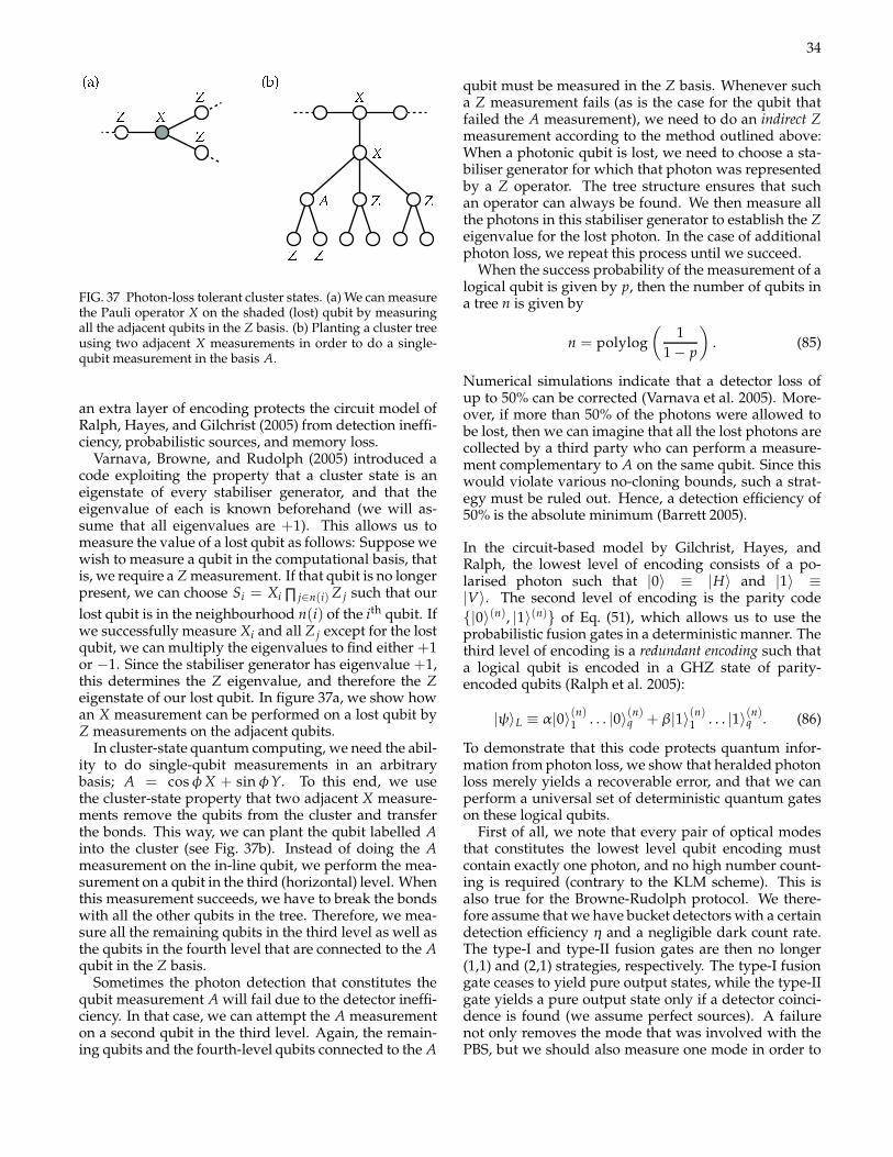
34

FIG. 37 Photon-loss tolerant cluster states. (a) We can measurethe Pauli operator X on the shaded (lost) qubit by measuringall the adjacent qubits in the Z basis. (b) Planting a cluster treeusing two adjacent X measurements in order to do a single-qubit measurement in the basis A.

an extra layer of encoding protects the circuit model ofRalph, Hayes, and Gilchrist (2005) from detection ineffi-ciency, probabilistic sources, and memory loss.

Varnava, Browne, and Rudolph (2005) introduced acode exploiting the property that a cluster state is aneigenstate of every stabiliser generator, and that theeigenvalue of each is known beforehand (we will as-sume that all eigenvalues are +1). This allows us tomeasure the value of a lost qubit as follows: Suppose wewish to measure a qubit in the computational basis, thatis, we require a Z measurement. If that qubit is no longerpresent, we can choose Si = Xi ∏ j∈n(i) Z j such that our

lost qubit is in the neighbourhood n(i) of the ith qubit. Ifwe successfully measure Xi and all Z j except for the lostqubit, we can multiply the eigenvalues to find either +1or −1. Since the stabiliser generator has eigenvalue +1,this determines the Z eigenvalue, and therefore the Zeigenstate of our lost qubit. In figure 37a, we show howan X measurement can be performed on a lost qubit byZ measurements on the adjacent qubits.

In cluster-state quantum computing, we need the abil-ity to do single-qubit measurements in an arbitrarybasis; A = cosφX + sinφY. To this end, we usethe cluster-state property that two adjacent X measure-ments remove the qubits from the cluster and transferthe bonds. This way, we can plant the qubit labelled Ainto the cluster (see Fig. 37b). Instead of doing the Ameasurement on the in-line qubit, we perform the mea-surement on a qubit in the third (horizontal) level. Whenthis measurement succeeds, we have to break the bondswith all the other qubits in the tree. Therefore, we mea-sure all the remaining qubits in the third level as well asthe qubits in the fourth level that are connected to the Aqubit in the Z basis.

Sometimes the photon detection that constitutes thequbit measurement A will fail due to the detector ineffi-ciency. In that case, we can attempt the A measurementon a second qubit in the third level. Again, the remain-ing qubits and the fourth-level qubits connected to the A

qubit must be measured in the Z basis. Whenever sucha Z measurement fails (as is the case for the qubit thatfailed the A measurement), we need to do an indirect Zmeasurement according to the method outlined above:When a photonic qubit is lost, we need to choose a sta-biliser generator for which that photon was representedby a Z operator. The tree structure ensures that suchan operator can always be found. We then measure allthe photons in this stabiliser generator to establish the Zeigenvalue for the lost photon. In the case of additionalphoton loss, we repeat this process until we succeed.

When the success probability of the measurement of alogical qubit is given by p, then the number of qubits ina tree n is given by

n = polylog

(1

1 − p

). (85)

Numerical simulations indicate that a detector loss ofup to 50% can be corrected (Varnava et al. 2005). More-over, if more than 50% of the photons were allowed tobe lost, then we can imagine that all the lost photons arecollected by a third party who can perform a measure-ment complementary to A on the same qubit. Since thiswould violate various no-cloning bounds, such a strat-egy must be ruled out. Hence, a detection efficiency of50% is the absolute minimum (Barrett 2005).

In the circuit-based model by Gilchrist, Hayes, andRalph, the lowest level of encoding consists of a po-larised photon such that |0〉 ≡ |H〉 and |1〉 ≡|V〉. The second level of encoding is the parity code

|0〉(n), |1〉(n) of Eq. (51), which allows us to use theprobabilistic fusion gates in a deterministic manner. Thethird level of encoding is a redundant encoding such thata logical qubit is encoded in a GHZ state of parity-encoded qubits (Ralph et al. 2005):

|ψ〉L ≡ α|0〉(n)1 . . . |0〉(n)

q +β|1〉(n)1 . . . |1〉(n)

q . (86)

To demonstrate that this code protects quantum infor-mation from photon loss, we show that heralded photonloss merely yields a recoverable error, and that we canperform a universal set of deterministic quantum gateson these logical qubits.

First of all, we note that every pair of optical modesthat constitutes the lowest level qubit encoding mustcontain exactly one photon, and no high number count-ing is required (contrary to the KLM scheme). This isalso true for the Browne-Rudolph protocol. We there-fore assume that we have bucket detectors with a certaindetection efficiency η and a negligible dark count rate.The type-I and type-II fusion gates are then no longer(1,1) and (2,1) strategies, respectively. The type-I fusiongate ceases to yield pure output states, while the type-IIgate yields a pure output state only if a detector coinci-dence is found (we assume perfect sources). A failurenot only removes the mode that was involved with thePBS, but we should also measure one mode in order to

35

purify the cluster. Hence, the type-II fusion gate withbucket detectors is a (2,2)-strategy, and the growth re-quirement is m > 2/p.

Suppose we wish to measure the value of the logicalqubit |ψ〉L in the computational basis (as we discuss be-low, any other measurement can be performed by firstapplying a single-qubit rotation to |ψ〉L). Since the log-ical qubit is a GHZ state, it is sufficient to measure onlyone parity qubit, e.g., the first one. Physically, this mea-surement constitutes a counting of horizontally and ver-tically polarised photons: if the number of verticallypolarised photons is even, then the value of the parity

qubit is |0〉(n)1 , and if it is odd, then its value is |1〉(n)

1 . Inorder to successfully establish the parity, we thereforeneed to detect all n photons.

When we include photon loss in this measurement,there are three possible measurement outcomes for ev-ery optical mode: “horizontal”, “vertical”, or “detectorfailure”. In the language of POVMs, this can be writtenas

E(H) = η|H〉〈H| ;

E(V) = η|V〉〈V| ;

E(0) = (1 − η) (|H〉〈H|+ |V〉〈V|) . (87)

These POVMs add up to unity in the subspace spannedby |H〉 and |V〉, as required. A particular measurementoutcome on n modes can then be written as a string ofn outcomes s = (s1, . . . , sn), where every si ∈ H, V, 0.The optical state after finding a particular measurementoutcome s is then

ρ2...q = Tr1

[E

(s)1 |ψ〉L〈ψ|

]. (88)

When all photons are detected, the qubit is projectedonto its logical value. However, when one or morequbits are lost it is no longer possible to establish theparity. Therefore, as soon as a photon is lost the nextphoton is measured in a diagonal basis, thus disentan-gling the parity qubit from the other parity qubits. Afew lines of algebra shows that the remaining q − 1 par-ity qubits are in the state

|ψ〉′L = α|0〉(n)2 . . . |0〉(n)

q +β|1〉(n)2 . . . |1〉(n)

q . (89)

In other words, the encoding has become smaller but thequantum information has not been erased. We can there-fore retry the measurement of the qubit q times.

Next, we have to show that we can perform determin-istic one- and two-qubit gates using this redundant en-coding. To this end, recall how deterministic gates wereimplemented in the parity encoding: A universal set of

gates is X(p)θ , Z(p), Z

(p)π/2

, CNOT(p). We added a super-

script (p) to indicate that these gates act on the parity

qubit. As we have seen, the gates Z(p)π/2

and CNOT(p)

cannot be implemented deterministically, and have tobe built using fusion gates.

How can these gates be used to form a universal seton the redundantly encoded (logical) qubit? First, thesingle-qubit gate Z is still implemented deterministi-

cally: Z = Z(p) = nσz. Therefore, in order to ap-ply a Z gate, a σz operation must be applied to all nphotons in one and only one parity qubit. Secondly, thegate Zπ/2 is diagonal in the computational basis, and

can therefore be implemented using one Z(p)π/2

. Thirdly,

the Xθ gate on the redundantly encoded qubit is some-what problematic, since the gate transforms separablestates of parity qubits into highly entangled GHZ states.

However, if we apply (q− 1) CNOT(p) gates, we can de-

code the qubit such that its state is (α|0〉(n)1 +β|1〉(n)

1 ) ⊗|0〉(n)

2 . . . |0〉(n)q . We can then apply the deterministic gate

X(p)θ to the first parity qubit, and use another set of

(q− 1) CNOT(p) gates to re-encode the qubit. Therefore,

the gate Xθ “costs” 2(q − 1) CNOT(p) gates. Finally, theCNOT gate on the redundantly encoded qubit can be

implemented using q CNOT(p) gates.

Since every single-qubit operation can be constructedfrom Xθ and Zπ/2, we can perform arbitrary single-qubit

measurements. We now have a universal set of gateson our logical qubit, together with computational-basisread out and an efficient encoding mechanism. Nu-merical simulations indicate that this method allows forcombined detector, source and memory efficiencies ofη > 55% (Ralph et al. 2005).

Note that there seem to be conflicting requirementsin this code: In order to execute successful fusion gates,we want n to be reasonably large. On the other hand,we want n to be as small as possible such that the prob-ability of measuring all n photons p = ηn is not toosmall. We assumed that every parity qubit is encodedwith the same number of photons n, but this is not nec-essary. In principle, this method works when differentparity qubits have different-sized encodings. However,some care should be taken to choose every ni as close tothe optimal value as possible.

B. General error correction in LOQC

As we mentioned before, photon loss is not the only er-ror in LOQC, and creating large cluster trees or a sizableredundant encoding in the circuit model will actuallyamplify other errors, such as dephasing. A truly fault-tolerant quantum computer architecture must thereforebe able to handle the actual physical noise that will bepresent. Given a certain noise model and error correct-ing codes, we can derive fault-tolerant thresholds: Theerrors must be smaller than the threshold value for con-catenated error correction to eliminate them all. Knillet al. (2000) considered a combination of photon lossand dephasing in the original KLM proposal and foundthat the accuracy threshold for the optical components

36

in that scheme was higher than 99%.Dawson, Haselgrove, and Nielsen (2006a,b) per-

formed an extensive numerical study of fault-tolerantthresholds for linear optical cluster state quantum com-puting. The computational model they adopted isNielsen’s micro-cluster approach, described in sectionIII.C, with type-I fusion gates instead of KLM-type CZgates. The physical operations in this model are Bell-state preparation, single-photon gates and memories,type-I fusion gates, and photon measurements. Thecomputation proceeds in time steps, with exactly oneoperation at each step. Furthermore, it is assumed thatany two single-photon qubits in the computation canserve as the inputs of the fusion gate. In other words,we have a direct interaction between qubits. In addition,parallel operations are allowed to speed up the com-putation and minimise the use of quantum memories.Finally, the classical computation needed to control thecluster state computing is taken to be sufficiently fast.

The noise model adopted by Dawson et al. consistsof the inherent probabilistic nature of the fusion gates,as well as photon loss and depolarisation at every timestep in the computation. The photon loss is charac-terised by a uniform loss probability γ, and the depolar-isation comes in two flavours: Single-qubit operationshave a probability ǫ/3 of undergoing a Pauli operationX, Y, or Z. After the Bell-state preparation and beforethe fusion gate input, the two photons undergo a corre-lated depolarising noise: With probability (1 −ǫ) noth-ing happens to the qubits, while with probability ǫ/15any of the remaining 15 two-qubit Pauli operators areapplied. This is a completely general model for the noisethat can affect optical cluster state quantum computing,and the resulting fault-tolerance simulation gives an ac-curacy threshold region onγ andǫ. Thresholds were ob-tained for both a seven-qubit CSS error correction codeand a 23-qubit Golay error correction code. The studyshows that scalable quantum computing with the 23-qubit code is possible for a maximum loss probability of

γ < 3 · 10−3 and a maximum depolarising probability

of ǫ < 10−4.Even though this noise model accounts for general

noise, and the fault-tolerant threshold puts a boundon its magnitude, it is clearly a simplification of thephysical noise that is expected in cluster state LOQC.It is argued that the difference between correlated two-qubit noise and independent noise does not changethe threshold much. Similarly, using one parameterto describe both photon absorption and detector effi-ciency will not have a dramatic effect on the thresh-old (Nielsen 2006). The next milestone for establishingfault-tolerance thresholds is to adopt a noise model inwhich the parameters are measurable quantities, suchas the visibility in a Hong-Ou-Mandel experiment andphoton loss probabilities.

When various parameters in a noise model differ sig-nificantly, it might be beneficial to diversify the errorcorrection codes. EC codes that correct specific errors

such as photon loss or depolarisation may be smallerthan generic EC codes, and therefore introduce lessnoise. A round of special error correction might be usedto reduce large errors, and subsequent generic error cor-rection will further reduce the errors below the fault-tolerant threshold.

In addition, certain types of errors or noise might benaturally suppressed by a suitable alteration in the ar-chitecture. For example, there is a way to create high-fidelity four-photon GHZ states with lossy bucket de-tectors and inefficient sources (Gilchrist 2005). Assumethat the Bell-pair source creates a state of the formps|0〉〈0| + (1 − ps)|Ψ−〉〈Ψ−|, where |Ψ−〉 is the two-photon polarization singlet state. This is a reasonableerror model when the source obeys selection rules thatprevent single-photon components to contribute to theoutput state (c.f., Benson et al. 2000). In order to makea three-photon GHZ state using these sources we usea type-I fusion gate and post-select on a single detectorclick. The detector click indicates that at least one sourcecreated a photon pair. However, if only one photon pairwas created, the output mode of the type-I fusion gatemust necessarily empty. By taking the output modesof two type-I fusion gates in two separate three-photonGHZ creation attempts, and leading them into a type-IIfusion gate, we can post-select on finding two detectorclicks. As a result, high-fidelity four-photon GHZ statesare produced.

Several other specialised circuits have been proposedthat either detect errors or correct them. For exam-ple, Ralph (2003) proposed a simple demonstrationcircuit that detects and corrects bit flip errors on asingle qubit using the encoded qubit state α|0〉|0〉 +β|1〉|1〉 and an ancilla qubit |0〉. However, since thisis a probabilistic protocol, this circuit cannot naivelybe inserted in a quantum computing circuit. If weassume the availability of perfectly efficient detectors(not necessarily photon-number resolving), determin-istic polarisation-flip detection for distributing entan-glement can be achieved (Kalamidas 2004). In a sim-ilar fashion, a single-qubit error correction circuit canbe constructed with polarising beam splitters, half-waveplates, and Pockels cells (Kalamidas 2005). Here, we as-sume that these passive optical elements do not induceadditional noise. A full analysis would have to take thisnoise into account.

VI. OUTLOOK: BEYOND LINEAR OPTICS

We have seen in this review that it is possible to con-struct a quantum computer with linear optics, single-photon sources, and photon detection alone. Knill,Laflamme, and Milburn (2001) overturned the conven-tional wisdom that a lack of direct photon-photon inter-actions prohibits scalability. Since KLM, several groupshave proposed modifications to building a linear opticalquantum computer with reduced resources and realistic

37

(noisy) components.

The basic principles of LOQC have all been demon-strated experimentally, predominantly using parametricdown-conversion (PDC) and bucket photon detection.Due to the small efficiency of PDC photon sources, how-ever, these techniques cannot be considered scalable ina practical sense. Currently, there is a concerted effort tobuild the necessary single-photon sources, photon de-tectors, and quantum memories for a scalable linear op-tical quantum computer. On the theoretical front, thereis an ongoing effort to design more efficient architec-tures and effective error correction codes tailored to thenoise model that is relevant to LOQC.

Nevertheless, constructing the necessary componentsand using fault-tolerant encoding is hard, and severalextensions to LOQC have been proposed. In this lastsection we sketch a few additions to the linear opticaltoolbox that can make quantum computing a little biteasier.

First, we have seen in section I.D that a cross-Kerrnonlinearity can be used to induce a photon-photon in-teraction, and how two-qubit quantum gates can be con-structed using such a nonlinearity. Unfortunately, natu-ral Kerr nonlinearities are extremely small, and this isnot a practical method for creating optical gates. How-ever, recently it was suggested that a small nonlinear-ity might still be used for quantum computing. It wasshown by Munro et al. (2005) how such nonlinearitiescan make a number-resolving QND detector, and Barrettet al. (2005) showed how a small cross-Kerr nonlinear-ity can be used to perform complete Bell measurementswithout destroying the photons. Subsequently, it wasrealized by Nemoto and Munro (2004) that this tech-nique can also be used to create a deterministic CNOTgate on photonic qubits. Recent work in electromagnet-ically induced transparencies by Lukin and Imamoglu(2000, 2001) suggests that the small-but-not-tiny nonlin-earities needed for this method are on the threshold ofbecoming practical. Alternatively, relatively large non-linearities can be obtained in photonic band-gap materi-als (Friedler et al. 2004).

Secondly, if we have high-fidelity single-photonsources and memories, it might become beneficial to en-gineer these systems such that they support coherentsingle-qubit operations. This way, we can redefine ourqubits as isolated static systems, and we have circum-vented the problem of qubit loss. When these matterqubits emit a qubit-dependent photon, they can in turnbe entangled using techniques from linear optical quan-tum computing. It was shown by Barrett and Kok (2005)that such an architecture can support scalable quantumcomputing, even with current realistic components. In-dependently, Lim et al. (2005) showed how a similarsetup can be used to implement deterministic two-qubitquantum gates. Recently, these two methods were com-bined in a fault tolerant, near-deterministic quantumcomputer architecture (Lim et al. 2005a).

Thirdly, Franson, Jacobs, and Pittman proposed the

implementation of a two-qubit√

SWAP gate using thequantum Zeno effect: Two optical fibres are fused andsplit again, such that the input modes overlap in a smallsection of the fibre. This acts as a beam splitter on themodes in the input and output fibres. At regular inter-vals inside the joint fibre we place atoms with a two-photon transition. This transition acts as a two-photonmeasurement, while single-photon wave-packets prop-agate through the fibre undisturbed. Furthermore, thesingle-photon wave-packets maintain coherence. Theeffect of this repeated two-photon measurement is tosuppress the Hong-Ou-Mandel effect via the quantumZeno effect. In this way, two single-photon qubits inthe input modes are transformed into two single-photon

qubits in the output modes and undergo a√

SWAP gate.

Finally, an alternative approach to linear optical quan-tum computing involves encoding qubits in squeezedor coherent states of light (Gottesman et al. 2001;Ralph et al. 2003). Linear elements take on a new ca-pability in these implementations. For example Bellmeasurements and fan-out gates become deterministicelements (van Enk and Hirota 2002; Jeong et al. 2001).The downside is that it is difficult to produce thesuperposition states that are required as resourcesin such schemes, although considerable theoreticaland experimental progress has been made recently(Lund et al. 2004; Wenger et al. 2004). If this problem issolved, considerable savings in resources could resultfrom adopting such implementations.

Whatever the ultimate architecture of quantum com-puters will be, there will always remain a task for (lin-ear) optical quantum information processing: In orderto distribute quantum information over a network ofquantum computers, the qubit of choice will most likelybe optical. We therefore believe that the techniques re-viewed here are an important step towards full-scaledistributed quantum computing — the Quantum Inter-net.

Acknowledgements

We would like to thank James Franson, Andrew White,Geoff Pryde, Philip Walther, and their co-workers forproviding us with the experimental data of their respec-tive CNOT gates, and Charles Santori for allowing usto reproduce his figures. PK wishes to thank Sean Bar-rett and Dan Browne for stimulating discussions, RaduIonicioiu, Michael Raymer, and Colin Williams for valu-able comments, and Michael Nielsen for extensive cor-respondence on fault-tolerance in LOQC. This work wassupported by ARO, the Australian Centre for QuantumComputer Technology, DTO, the Hearne Institute, JSPS,LSU BOR-LINK, MIC, NSA, the QIPIRC, and the EURAMBOQ Project.

38

References

[Achilles et al. 2003] D. Achilles, C. Silberhorn, C. Sliwa,K. Banaszek, and I. A. Walmsley, Opt. Lett., 28 2387, 2003.

[Adami and Cerf 1999] C. Adami and N. J. Cerf, Lect. NotesComput. Sc., 1509 391, 1999.

[Banaszek and Walmsley 2003] K. Banaszek and I. A. Walms-ley, Opt. Lett., 28 52, 2003.

[Barnett et al. 1989] S. M. Barnett, J. Jeffers, A. Gatti, andR. Loudon, Phys. Rev. A, 57 2134, 1989.

[Barreiro et al. 2005] J. T. Barreiro, N. K. Langford, N. A. Pe-ters, and P. G. Kwiat, Phys. Rev. A, 72 060310, 2005.

[Barrett and Kok 2005] S. D. Barrett and P. Kok, Phys. Rev. A,72 060310, 2005.

[Barrett et al. 2005] S. D. Barrett, P. Kok, K. Nemoto, R. G.Beausoleil, W. J. Munro, and T. P. Spiller, Phys. Rev. A,72 060302, 2005.

[Barrett 2005] S. D. Barrett, Private communication, 2005.[Benson et al. 2000] O. Benson, C. Santori, M. Pelton, and

Y. Yamamoto, Phys. Rev. Lett., 84 2513, 2000.[Bergou et al. 2000] J. A. Bergou, M. Hillery, and Y. Q. Sun, J.

Mod. Opt., 47 487, 2000.[Berry et al. 2004] D. W. Berry, S. Scheel, C. R. Meyers, B. C.

Sanders, P. L. Knight, and R. Laflamme, New J. Phys., 6 93,2004.

[Berry et al. 2005] D. W. Berry, S. Scheel, B. C. Sanders, andP. L. Knight, Phys. Rev. A, 69 031806, 2005.

[Beveratos et al. 2002] A. Beveratos, S. Kuhn, R. Brouri,T. Gacoin, J. P. Poizat, and P. Grangier, Eur. Phys. J. D,18 191, 2002.

[Biedenharn and Louck 1981] L. C. Biedenharn and J. D.Louck, Angular Momentum in Quantum Physics (Encyclope-dia of Mathematics and Its Applications 8), Addison-Wesley,1981.

[Boschi et al. 1998] D. Boschi, S. Branca, F. D. Martini,L. Hardy, and S. Popescu, Phys. Rev. Lett., 80 1121, 1998.

[Branczyk et al. 2003] A. M. Branczyk, T. J. Osborne,A. Gilchrist, and T. C. Ralph, Phys. Rev. A, 68 043821,2003.

[Braunstein and Mann 1996] S. L. Braunstein and A. Mann,Phys. Rev. A, 51 R1727, 1996.

[Braunstein and van Loock 2005] S. L. Braunstein and P. vanLoock, Rev. Mod. Phys., 77 513, 2005.

[Brokmann et al. 2004] X. Brokmann, G. Messin, P. Desbiolles,E. Giacobino, M. Dahan, and J. P. Hermier, New J. Phys., 699, 2004.

[Browne and Rudolph 2005] D. E. Browne and T. Rudolph,Phys. Rev. Lett., 95 010501, 2005.

[Brune et al. 1990] M. Brune, S. Haroche, V. Lefevre, J. Rai-mond, and N. Zagury, Phys. Rev. Lett., 65 976, 1990.

[Brune et al. 1992] M. Brune, S. Haroche, J. M. Raimond,L. Davidovich, and N. Zagury, Phys. Rev. A, 45 5193, 1992.

[Brunel et al. 1999] C. Brunel, B. Lounis, P. Tamarat, andM. Orrit, Phys. Rev. Lett., 83 2722, 1999.

[Calsamiglia 2002] J. Calsamiglia, Phys. Rev. A, 65 030301,2002.

[Cerf et al. 1998] N. J. Cerf, C. Adami, and P. G. Kwiat, Phys.Rev. A, 57 R1477, 1998.

[Chuang and Nielsen 1997] I. L. Chuang and M. A. Nielsen, J.Mod. Phys., 44 2455, 1997.

[Chuang and Yamamoto 1995] I. L. Chuang and Y. Yamamoto,Phys. Rev. A, 52 3489, 1995.

[Cinelli et al. 2005] C. Cinelli, M. Barbieri, F. D. Martini, and

P. Mataloni, Laser Phys., 15 124, 2005.[Clausen et al. 2002] J. Clausen, L. Knoll, and D. G. Welsch, J.

Opt. B, 4 155, 2002.[Clausen et al. 2003] J. Clausen, L. Knoll, and D. G. Welsch,

Phys. Rev. A, 68 043822, 2003.[Clauser and Dowling 1996] J. F. Clauser and J. P. Dowling,

Phys. Rev. A, 53 4587, 1996.[d’Ariano et al. 2000] G. M. d’Ariano, C. Macchiavello, and

L. Maccone, Fortschr. Phys., 48 573, 2000.[Dawson et al. 2006a] C. M. Dawson, H. L. Haselgrove, and

M. A. Nielsen, Phys. Rev. Lett., 96 020501, 2006.[Dawson et al. 2006b] C. M. Dawson, H. L. Haselgrove, and

M. A. Nielsen, quant-ph/0601066, 2006.[De Martini et al. 2005] F. De Martini, G. Di Giuseppe, and M.

Marrocco, Phys. Rev. Lett., 76 900, 1996.[de Riedmatten et al. 2003] H. de Riedmatten, I. Marcikic,

W. Tittel, H. Zbinden, and N. Gisin, Phys. Rev. A, 67022301, 2003.

[Deuar and Munro 2000a] P. Deuar and W. J. Munro, Phys.Rev. A, 61 010306, 2000.

[Deuar and Munro 2000b] P. Deuar and W. J. Munro, Phys.Rev. A, 62 042304, 2000.

[Dowling 1998] J. P. Dowling, IEEE Proc. Opt. Elec., 145 420,1998.

[Eisert 2005] J. Eisert, Phys. Rev. Lett., 95 040502, 2005.[Ekert 1998] A. Ekert, Phys. Scripta, T76 218, 1998.[Englert et al. 2001] B. G. Englert, C. Kurtsiefer, and H. Wein-

furter, Phys. Rev. A, 63 032303, 2001.[Fearn and Loudon 1987] H. Fearn and R. Loudon, Opt. Com-

mun., 64 485, 1987.[Fiorentino and Wong 2004] M. Fiorentino and F. N. C. Wong,

Phys. Rev. Lett., 93 070502, 2004.[Fitch et al. 2003] M. J. Fitch, B. C. Jacobs, T. B. Pittman, and

J. D. Franson, Phys. Rev. A, 68 043814, 2003.[Fleischhauer and Lukin 2002] M. Fleischhauer and M. D.

Lukin, Phys. Rev. A, 65 022314, 2002.[Franson and Pittman 1999] J. D. Franson and T. B. Pittman,

Lect. Notes Comput. Sc., 1509 383, 1999.[Franson et al. 2002] J. D. Franson, M. M. Donegan, M. J. F. B.

Jacobs, and T. B. Pittman, Phys. Rev. Lett., 89 137901, 2002.[Franson et al. 2003] J. D. Franson, B. C. Jacobs, and T. B.

Pittman, Fortschr. Phys., 51 369, 2003.[Friedler et al. 2004] I. Friedler, G. Kurizki, and D. Petrosyan,

Europhys. Lett., 68 625, 2004.[Gaebel et al. 2004] T. Gaebel, I. Popa, A. Gruber, M. Domhan,

F. Jelezko, and J. Wrachtrup, N. J. Phys., 6 98, 2004.[Gasparoni et al. 2004] S. Gasparoni, J. W. Pan, P. Walther,

T. Rudolph, and A. Zeilinger, Phys. Rev. Lett., 93 020504,2004.

[Gerard et al. 2002] J. M. Gerard, I. Robert, E. Moreau, M. Gal-lart, and I. Abram, J. Phys. IV, 12 29, 2002.

[Giacomini et al. 2003] S. Giacomini, F. Sciarrino, E. Lombardi,and F. De Martini, Phys. Rev. A, 66 030302, 2002.

[Gilchrist 2005] A. Gilchrist, private communication to Dan E.Browne.

[Gilchrist et al. 2003] A. Gilchrist, W. J. Munro, and A. G.White, Phys. Rev. A, 67 040304, 2003.

[Gilchrist et al. 2005] A. Gilchrist, A. J. F. Hayes, and T. C.Ralph, quant-ph/0505125, 2005.

[Gingrich et al. 2003] R. M. Gingrich, P. Kok, H. Lee, F. Vatan,and J. P. Dowling, Phys. Rev. Lett., 91 217901, 2003.

[Glancy et al. 2002] S. Glancy, J. M. LoSecco, H. M. Vasconce-los, and C. E. Tanner, Phys. Rev. A, 65 062317, 2002.

[Gottesman and Chuang 1999] D. Gottesman and I. L.

39

Chuang, Nature, 402 390, 1999.[Gottesman et al. 2001] D. Gottesman, A. Kitaev, and

J. Preskill, Phys. Rev. A, 64 012310, 2001.[Gottesman 1999] D. Gottesman, The Heisenberg Representation

of Quantum Computers, Group 22: Proceedings of the XXIIInternational Colloquium on Group Theoretical Methodsin Physics, Cambridge, MA, International Press, 1999.

[Grangier et al. 1998] P. Grangier, J. A. Levenson, and J. P.Poizat, Nature, 396 537, 1998.

[Greulich and Thiel 2001] K. O. Greulich and E. Thiel, SingleMol., 2 5, 2001.

[Grice et al. 2001] W. P. Grice, A. B. U’Ren, and I. A. Walmsley,Phys. Rev. A, 64 063815, 2001.

[Hayes et al. 2004] A. J. F. Hayes, A. Gilchrist, C. R. Myers, andT. C. Ralph, J. Opt. B, 6 533, 2004.

[Hein et al. 2004] M. Hein, J. Eisert, and H. J. Briegel, Phys.Rev. A, 69 062311, 2004.

[Hennrich et al. 2004] M. Hennrich, T. Legero, A. Kuhn, andG. Rempe, New J. Phys., 6 86, 2004.

[Hockney et al. 2003] G. M. Hockney, P. Kok, and J. P. Dowl-ing, Phys. Rev. A, 67 032306, 2003.

[Hofmann and Takeuchi 2002] H. F. Hofmann andS. Takeuchi, Phys. Rev. A, 66 024308, 2002.

[Hofmann et al. 2003] H. F. Hofmann, K. Kojima, S. Takeuchi,and K. Sasaki, J. Opt. B, 5 218, 2003.

[Hollars et al. 2003] C. W. Hollars, S. M. Lane, and T. Huser,Chem. Phys. Lett., 370 393, 2003.

[Hong et al. 1987] C. K. Hong, Z. Y. Ou, and L. Mandel, Phys.Rev. Lett., 59 2044, 1987.

[Hours et al. 2003] J. Hours, S. Varoutsis, M. Gallart, J. Bloch,I. Robert-Philip, A. Cavanna, I. Abram, F. Laruelle, andJ. M. Gerard, Appl. Phys. Lett., 82 2206, 2003.

[Howell and Yeazell 2000a] J. C. Howell and J. A. Yeazell,Phys. Rev. A, 62 032311, 2000.

[Howell and Yeazell 2000b] J. C. Howell and J. A. Yeazell,Phys. Rev. Lett., 85 198, 2000.

[Howell and Yeazell 2000c] J. C. Howell and J. A. Yeazell,Phys. Rev. A, 61 052303, 2000.

[Hutchinson and Milburn 2004] G. D. Hutchinson and G. J.Milburn, J. Mod. Opt., 51 1211, 2004.

[Imamoglu 2002] A. Imamoglu, Phys. Rev. Lett., 89 163602,2002.

[Imoto et al. 1985] N. Imoto, H. A. Haus, and Y. Yamamoto,Phys. Rev. A, 32 2287, 1985.

[Jacobs et al. 2002] B. C. Jacobs, T. B. Pittman, and J. D. Fran-son, Phys. Rev. A, 66 052307, 2002.

[James and Kwiat 2002] D. F. V. James and P. G. Kwiat, Phys.Rev. Lett., 89 183601, 2002.

[Jelezko et al. 2002] F. Jelezko, I. Popa, A. Gruber, C. Tietz, andJ. Wrachtrup, Appl. Phys. Lett., 81 2160, 2002.

[Jeong et al. 2001] H. Jeong, M. S. Kim, and J. Lee, Phys. Rev.A, 64 052308, 2001.

[Jex et al. 1995] I. Jex, S. Stenholm, and A. Zeilinger, Opt.Commun., 117 95, 1995.

[Johnsson and Fleischhauer 2003] M. Johnsson and M. Fleis-chhauer, Phys. Rev. A, 67 061802, 2003.

[Julsgaard et al. 2004] B. Julsgaard, J. Sherson, J. I. Cirac,J. Fiurasek, and E. S. Polzik, Nature, 432 482, 2004.

[Kalamidas 2004] D. Kalamidas, Phys. Lett. A, 321 87, 2004.[Kalamidas 2005] D. Kalamidas, Phys. Lett. A, 343 331, 2005.[Keller et al. 2004] M. Keller, B. Lange, K. Hayasaka,

W. Lange, and H. Walther, Nature, 431 1075, 2004.[Kim et al. 1999] J. Kim, S. Takeuchi, Y. Yamamoto, and H. H.

Hogue, Appl. Phys. Lett., 74 902, 1999.

[Kiraz et al. 2004] A. Kiraz, M. Atature, and A. Imamoglu,Phys. Rev. A, 69 032305, 2004.

[Knill et al. 2000] E. Knill, R. Laflamme, and G. J. Milburn,quant-ph/0006120, 2000.

[Knill et al. 2001] E. Knill, R. Laflamme, and G. J. Milburn, Na-ture, 409 46, 2001.

[Knill 2002] E. Knill, Phys. Rev. A, 66 052306, 2002.[Knill 2003] E. Knill, Phys. Rev. A, 68 064303, 2003.[Knill 2005] E. Knill, Nature, 434 39, 2005.[Koashi et al. 2001] M. Koashi, T. Yamamoto, and N. Imoto,

Phys. Rev. A, 63 030301, 2001.[Kok and Braunstein 2000a] P. Kok and S. L. Braunstein, Phys.

Rev. A, 62 064301, 2000.[Kok and Braunstein 2000b] P. Kok and S. L. Braunstein, Phys.

Rev. A, 61 042304, 2000.[Kok and Braunstein 2001] P. Kok and S. L. Braunstein, Phys.

Rev. A, 63 033812, 2001.[Kok and Braunstein 2006] P. Kok and S. L. Braunstein, In-

ternational Journal of Quantum Information (in press),quant-ph/0407259.

[Kok and Munro 2005] P. Kok and W. J. Munro, Phys. Rev.Lett., 95 048901, 2005.

[Kok et al. 2002] P. Kok, H. Lee, and J. P. Dowling, Phys. Rev.A, 66 063814, 2002.

[Kok 2003] P. Kok, IEEE: Sel. Top. Quantum Electronics, 91498, 2003.

[Kuhn et al. 2002] A. Kuhn, M. Hennrich, and G. Rempe,Phys. Rev. Lett., 89 067901, 2002.

[Kurtsiefer et al. 2000] C. Kurtsiefer, S. Mayer, P. Zarda, andH. Weinfurter, Phys. Rev. Lett., 85 290, 2000.

[Kuzmich et al. 2003] A. Kuzmich, W. P. Bowen, A. D. Boozer,A. Boca, C. W. Chou, L. M. Duan, and H. J. Kimble, Nature,423 731, 2003.

[Kwiat and Weinfurter 1998] P. G. Kwiat and H. Weinfurter,Phys. Rev. A, 58 R2623, 1998.

[Kwiat et al. 2000] P. G. Kwiat, J. R. Mitchell, P. D. D.Schwindt, and A. G. White, J. Mod. Opt., 47 257, 2000.

[Lapaire et al. 2003] G. G. Lapaire, P. Kok, J. P. Dowling, andJ. E. Sipe, Phys. Rev. A, 68 042314, 2003.

[Lee et al. 2004a] H. Lee, U. Yurtsever, P. Kok, G. M. Hockney,C. Adami, S. L. Braunstein, and J. P. Dowling, J. Mod Opt.,51 1517, 2004.

[Lee et al. 2004b] T. H. Lee, P. Kumar, A. Mehta, K. Xu, R. M.Dickson, and M. D. Barnes, Appl. Phys. Lett., 85 100, 2004.

[Leonhardt and Neumaier 2004] U. Leonhardt and A. Neu-maier, J. Opt. B, 6 L1, 2004.

[Leonhardt 2003] U. Leonhardt, Rep. Prog. Phys., 66 1207,2003.

[Leung 2004] D. W. Leung, Int. J. Quant. Inf., 2 33, 2004.[Li et al. 2005] X. Li, P. L. Voss, J. Chen, J. E. Sharping, and

P. Kumar, Opt. Lett., 30 1201, 2005.[Lim et al. 2005a] Y. L. Lim, S. D. Barrett, A. Beige, P. Kok, and

L. C. Kwek, Phys. Rev. A, 73 012304, 2006.[Lim et al. 2005b] Y. L. Lim, A. Beige, and L. C. Kwek, Phys.

Rev. Lett., 95 030505, 2005.[Lloyd 1995] S. Lloyd, Phys. Rev. Lett, 75 346, 1995.[Lombardi et al. 2002] E. Lombardi, F. Sciarrino, S. Popescu,

and F. De Martini, Phys. Rev. Lett, 88 070402, 2002.[Lounis and Moerner 2000] B. Lounis and W. E. Moerner, Na-

ture, 407 491, 2000.[Lounis and Orrit 2005] B. Lounis and M. Orrit, Rep. Prog.

Phys., 68 1129, 2005.[Lounis et al. 2000] B. Lounis, H. A. Bechtel, D. Gerion,

P. Alivisatos, and W. E. Moerner, Chem. Phys. Lett.., 329

40

399, 2000.[Lukin and Imamoglu 2000] M. D. Lukin and A. Imamoglu,

Phys. Rev. Lett., 84 1419, 2000.[Lukin and Imamoglu 2001] M. D. Lukin and A. Imamoglu,

Nature, 413 273, 2001.[Lund and Ralph 2002] A. P. Lund and T. C. Ralph, Phys. Rev.

A, 66 032307, 2002.[Lund et al. 2003] A. P. Lund, T. B. Bell, and T. C. Ralph, Phys.

Rev. A, 68 022313, 2003.[Lund et al. 2004] A. P. Lund, H. Jeong, T. C. Ralph, and

M. S. Kim, Phys. Rev. A, 70 020101, 2004.[Lutkenhaus et al. 1999] N. Lutkenhaus, J. Calsamiglia, and

K. A. Suominen, Phys. Rev. A, 59 3295, 1999.[Lvovsky and Raymer 1999] A. I. Lvovsky and M. G. Raymer,

quant-ph/0511044, 2005.[Maıtre et al. 1997] X. Maıtre, E. Hagley, G. Nogues, C. Wun-

derlich, P. Goy, M. Brune, J. M. Raimond, and S. Haroche,Phys. Rev. Lett., 79 769, 1997.

[Maurer et al. 2004] C. Maurer, C. Becher, C. Russo, J. Eschner,and R. Blatt, New J. Phys., 6 94, 2004.

[McKeefer et al. 2004] J. McKeefer, A. Boca, A. D. Boozer,R. Miller, J. R. Buck, A. Kuzmich, and H. J. Kimble, Sci-ence, 303 1992, 2004.

[Messin et al. 2001] G. Messin, J. P. Hermier, E. Giacobino,P. Desboilles, and M. Dahan, Opt. Lett., 26 1891, 2001.

[Michler et al. 2000] P. Michler, A. Kiraz, C. Becher, W. V.Schoenfeld, P. Petroff, L. D. Zhang, E. Hu, andA. Imamoglu, Science, 290 2282, 2000.

[Migdall et al. 2002] A. L. Migdall, D. Branning, and S. Castel-letto, Phys. Rev. A, 66 053805, 2002.

[Milburn 1989] G. J. Milburn, Phys. Rev. Lett., 62 2124, 1989.[Moreau et al. 2001] E. Moreau, I. Robert, L. Manin,

V. Thierry-Mieg, J. M. Gerard, and I. Abram, Phys.Rev. Lett., 87 183601, 2001.

[Munro et al. 2005] W. J. Munro, K. Nemoto, R. G. Beausoleil,and T. P. Spiller, Phys. Rev. A, 71 033819, 2005.

[Myers and Brandt 1997] J. M. Myers and H. E. Brandt, Meas.Sci, Technol., 8 1222, 1997.

[Myers and Laflamme] C. R. Myers and R. Laflamme, Lec-ture notes for the International School of Physics “EnricoFermi” on “Quantum Computers, Algorithms and Chaos”,Varenna, Italy, 2005; quant-ph/0512104.

[Nemoto and Braunstein 2002] K. Nemoto and S. L. Braun-stein, Phys. Rev. A, 66 032306, 2002.

[Nemoto and Munro 2004] K. Nemoto and W. J. Munro, Phys.Rev. Lett., 93 250502, 2004.

[Newton and Wigner 1949] T. D. Newton and E. P. Wigner,Rev. Mod. Phys., 21 400, 1949.

[Nielsen and Chuang 2000] M. A. Nielsen and I. L. Chuang,Quantum Computation and Quantum Information, Cam-bridge University Press, 2000.

[Nielsen and Dawson 2004] M. A. Nielsen and C. M. Dawson,Phys. Rev. A, 71 042323, 2004.

[Nielsen 2003] M. A. Nielsen, Phys. Lett. A, 308 96, 2003.[Nielsen 2004] M. A. Nielsen, Phys. Rev. Lett., 93 040503, 2004.[Nielsen 2005] M. A. Nielsen, quant-ph/0504097, 2005.[Nielsen 2006] M. A. Nielsen, private communication.[Nogues et al. 1999] G. Nogues, A. Rauschenbeutel, S. Os-

naghi, M. Brune, J. M. Raimond, and S. Haroche, Nature,400 239, 1999.

[O’Brien et al. 2003] J. L. O’Brien, G. J. Pryde, A. G. White,T. C. Ralph, and D. Branning, Nature, 426 264, 2003.

[O’Brien et al. 2004] J. L. O’Brien, G. J. Pryde, A. Gilchrist,D. F. V. James, N. K. Langford, T. C. Ralph, and A. G. White,

Phys. Rev. Lett., 93 080502, 2004.[O’Brien et al. 2005] J. L. O’Brien, G. J. Pryde, A. G. White, and

T. C. Ralph, Phys. Rev. A, 71 060303, 2005.[Paris et al. 2003] M. G. A. Paris, G. M. d’Ariano, P. L. Presti,

and P. Perinotti, Fortschr. Phys., 51 449, 2003.[Paris 2000] M. G. A. Paris, Phys. Rev. A, 62 033813, 2000.[Pelton et al. 2002] M. Pelton, C. Santori, J. Vuckovic, B. Y.

Zhang, G. S. Solomon, J. Plant, and Y. Yamamoto, Phys.Rev. Lett., 89 233602, 2002.

[Peres and Terno 2002] A. Peres and D. R. Terno J. Mod. Opt.,50 1165, 2003.

[Pittman and Franson 2002] T. B. Pittman and J. D. Franson,Phys. Rev. A, 66 062302, 2002.

[Pittman et al. 2002a] T. B. Pittman, B. C. Jacobs, and J. D.Franson, Phys. Rev. A, 66 052305, 2002.

[Pittman et al. 2002b] T. B. Pittman, B. C. Jacobs, and J. D.Franson, Phys. Rev. Lett., 88 257902, 2002.

[Pittman et al. 2002c] T. B. Pittman, B. C. Jacobs, and J. D.Franson, Phys. Rev. A, 66 042303, 2002.

[Pittman et al. 2003] T. B. Pittman, M. J. Fitch, B. C. Jacobs, andJ. D. Franson, Phys. Rev. A, 68 032316, 2003.

[Pittman et al. 2005] T. B. Pittman, B. C. Jacobs, and J. D. Fran-son, Phys. Rev. A, 71 052332, 2005.

[Pittmann et al. 2001] T. B. Pittmann, B. C. Jacobs, and J. D.Franson, Phys. Rev. A, 64 062311, 2001.

[Popescu 1995] S. Popescu, quant-ph/9501020, 1995.[Poyatos et al. 2001] J. F. Poyatos, J. I. Cirac, and P. Zoller,

Phys. Rev. Lett., 78 390, 1997.[Pryde et al. 2004] G. J. Pryde, J. L. O’Brien, A. G. White, S. D.

Bartlett, and T. C. Ralph, Phys. Rev. Lett., 92 190402, 2004.[Pryde et al. 2005] G. J. Pryde, J. L. O’Brien, A. G. White, S. D.

Bartlett, and T. C. Ralph, Phys. Rev. Lett., 95 048902, 2005.[Ralph et al. 2002a] T. C. Ralph, N. K. Langford, T. B. Bell, and

A. G. White, Phys. Rev. A, 65 062324, 2002.[Ralph et al. 2002b] T. C. Ralph, A. G. White, W. J. Munro, and

G. J. Milburn, Phys. Rev. A, 65 012314, 2002.[Ralph et al. 2003] T. C. Ralph, A. Gilchrist, G. Milburn,

W. Munro, and S. Glancy, Phys. Rev. A, 68 042319, 2003.[Ralph et al. 2005] T. C. Ralph, A. J. F. Hayes, and A. Gilchrist,

Phys. Rev. Lett., 95 100501, 2005.[Ralph 2003] T. C. Ralph, IEEE Sel. Top. Quantum Electronics,

9 1495, 2003.[Ralph 2004] T. C. Ralph, Phys. Rev. A, 70 012312, 2004.[Raussendorf and Briegel 2001] R. Raussendorf and H. J.

Briegel, Phys. Rev. Lett., 86 5188, 2001.[Raussendorf et al. 2003] R. Raussendorf, D. E. Browne, and

H. J. Briegel, Phys. Rev. A, 68 022312, 2003.[Raymer et al. 2005] M. G. Raymer, J. Noh, K. Banaszek, and

I. A. Walmsley, Phys. Rev. A, 72 023825, 2005.[Reck et al. 1994] M. Reck, A. Zeilinger, H. J. Bernstein, and

P. Bertani, Phys. Rev. Lett., 73 58, 1994.[Resch et al. 2002] K. J. Resch, J. S. Lundeen, and A. M. Stein-

berg, Phys. Rev. Lett., 89 037904, 2002.[Roch et al. 1997] J. F. Roch, K. Vigneron, P. Grelu, A. Sinatra,

J. P. Poizat, and P. Grangier, Phys. Rev. Lett., 78 634, 1997.[Rohde and Ralph 2005] P. P. Rohde and T. C. Ralph, Phys.

Rev. A, 71 032320, 2005.[Rohde et al. 2005] P. P. Rohde, T. C. Ralph, and M. A. Nielsen

Phys. Rev. A, 72 052332, 2005.[Rohde 2005] P. P. Rohde, J. Opt. B, 7 82, 2005.[Rosenberg et al. 2005] D. Rosenberg, A. E. Lita, A. J. Miller,

and S. W. Nam, Phys. Rev. A, 71 061803, 2005.[Rudolph and Pan 2001] T. Rudolph and J. W. Pan,

quant-ph/0108056, 2001.

41

[Sanaka et al. 2004] K. Sanaka, T. Jennewein, J. W. Pan,K. Resch, and A. Zeilinger, Phys. Rev. Lett., 92 017902,2004.

[Sanders and Rice 2000] B. C. Sanders and D. A. Rice, Phys.Rev. A, 61 013805, 2000.

[Santori et al. 2001] C. Santori, M. Pelton, G. S. Solomon,Y. Dale, and Y. Yamamoto, Phys. Rev. Lett., 86 1502, 2001.

[Santori et al. 2002a] C. Santori, D. Fattal, M. Pelton, G. S.Solomon, and Y. Yamamoto, Phys. Rev. B, 66 045308, 2002.

[Santori et al. 2002b] C. Santori, D. Fattal, J. Vuckovic, G. S.Solomon, and Y. Yamamoto, Nature, 419 594, 2002.

[Santori et al. 2004] C. Santori, D. Fattal, J. Vuckovic, G. S.Solomon, and Y. Yamamoto, New J. Phys., 6 89, 2004.

[Scheel and Audenaert 2005] S. Scheel and K. M. R. Aude-naert, New J. Phys., 7 149, 2005.

[Scheel and Lutkenhaus 2004] S. Scheel and N. Lutkenhaus,New J. Phys., 6 51, 2004.

[Scheel et al. 2003] S. Scheel, K. Nemoto, W. J. Munro, and P. L.Knight, Phys. Rev. A, 68 032310, 2003.

[Scheel et al. 2004] S. Scheel, J. Pachos, E. A. Hinds, and P. L.Knight, quant-ph/0403152, 2004.

[Scheel et al. 2005] S. Scheel, W. J. Munro, J. Eisert, K. Nemoto,and P. Kok, Phys. Rev. A, 73 034301, 2006.

[Scheel 2004] S. Scheel, quant-ph/0508189, 2005.[Scheel 2004] S. Scheel, quant-ph/0406127, 2005.[Schmidt and Imamoglu 1996] H. Schmidt and A. Imamoglu,

Opt. Lett., 21 1936, 1996.[Scully and Lamb 1969] M. O. Scully and W. E. Lamb, Phys.

Rev., 179 368, 1969.[Silva et al. 2005] M. Silva, M. Rotteler, and C. Zalka, Phys.

Rev. A, 72 032307, 2005.[Simon and Mukunda 1990] R. Simon and N. Mukunda,

Phys. Lett. A, 143 165, 1990.

[Sliwa and Banaszek 2003] C. Sliwa and K. Banaszek, Phys.Rev. A, 67 030101, 2003.

[Spedalieri et al. 2005] F. M. Spedalieri, H. Lee, and J. P. Dowl-ing, Phys. Rev. A, 73 012334, 2006.

[Spiller et al. 2005] T. P. Spiller, W. J. Munro, S. D. Barrett, andP. Kok, Cont. Phys., in press, 2005.

[Spreeuw 1998] R. J. C. Spreeuw, Found. Phys., 28 361, 1998.[Stace et al. 2003] T. M. Stace, G. J. Milburn, and C. H. W.

Barnes, Phys. Rev. B, 67 085317, 2003.[Steane 2003] A. M. Steane, Phys. Rev. A, 68 042322, 2003.[Stenholm 1996] S. Stenholm, Opt. Commun., 123 287, 1996.[Summhammer 1997] J. Summhammer, Phys. Rev. A, 56 4324,

1997.[Takeuchi et al. 1999] S. Takeuchi, J. Kim, Y. Yamamoto, and

H. H. Hogue, Appl. Phys. Lett., 74 1063, 1999.[Takeuchi 2000a] S. Takeuchi, Phys. Rev. A, 61 052302, 2000.[Takeuchi 2000b] S. Takeuchi, Phys. Rev. A, 62 032301, 2000.[Takeuchi 2001] S. Takeuchi, Electron. Comm. Jpn. 3, 84 52,

2001.[Thew et al. 2002] R. T. Thew, S. Tanzilli, W. Tittel, H. Zbinden,

and N. Gisin, Phys. Rev. A, 66 062304, 2002.[Torma and Stenholm 1996] P. Torma and S. Stenholm, Phys.

Rev. A, 54 4701, 1996.[Torma et al. 1995] P. Torma, S. Stenholm, and I. Jex, Phys.

Rev. A, 52 4853, 1995.

[Torma et al. 1996] P. Torma, I. Jex, and S. Stenholm, J. Mod.Opt., 43 245, 1996.

[Treussart et al. 2002] F. Treussart, R. Alleaume, V. L. Floc’h,L. T. Xiao, J. M. Courty, and J. F. Roch, Phys. Rev. Lett., 89093601, 2002.

[Turchette et al. 1995] Q. A. Turchette, C. J. Hood, W. Lange,H. Mabuchi, and H. J. Kimble, Phys. Rev. Lett., 75 4710,1995.

[U’Ren et al. 2003] A. B. U’Ren, K. Banaszek, and I. A. Walms-ley, Quant. Inf. Comput., 3 480, 2003.

[Vaidman and Yoran 1999] L. Vaidman and N. Yoran, Phys.Rev. A, 59 116, 1999.

[van Enk and Hirota 2002] S. J. van Enk and O. Hirota, Phys.Rev. A, 64 022313, 2002.

[van Loock and Lutkenhaus 2004] P. van Loock andN. Lutkenhaus, Phys. Rev. A, 69 012302, 2004.

[Varnava et al. 2005] M. Varnava, D. E. Browne, andT. Rudolph, quant-ph/0507036, 2005.

[Verstraete and Cirac 2004] F. Verstraete and J. I. Cirac, Phys.Rev. A, 70 060302, 2004.

[Vuckovic et al. 2003] J. Vuckovic, D. Fattal, C. Santori, andG. S. Solomon, Appl. Phys. Lett., 82 3596, 2003.

[Waks et al. 2003] E. Waks, K. Inoue, W. D. Oliver, E. Dia-manti, and Y. Yamamoto, IEEE: J. Sel. Top. Quantum Elec-tron., 9 1502, 2003.

[Walther et al. 2005] P. Walther, K. J. Resch, T. Rudolph, H. We-infurter, V. Vedral, M. Aspelmeyer, and A. Zeilinger, Na-ture, 434 169, 2005.

[Ward et al. 2005] M. B. Ward, O. Z. Karimov, D. C. Unitt, Z. L.Yuan, P. See, D. G. Gevaux, A. J. Shields, P. Atkinson, andD. A. Ritchie, Appl. Phys. Lett., 86 201111, 2005.

[Weihs et al. 1996] G. Weihs, M. Reck, H. Weinfurter, andA. Zeilinger, Opt. Lett., 21 302, 1996.

[Weinfurter 1994] H. Weinfurter, Europhysics Lett., 25 559,1994.

[Wenger et al. 2004] J. Wenger, R. Tualle-Brouri, and P. Grang-ier, Phys. Rev. Lett., 92 153601, 2004.

[Wightman 1962] A. S. Wightman, Rev. Mod. Phys., 34 845,1962.

[Yamamoto et al. 1988] Y. Yamamoto, M. Kitagawa, andK. Igeta, Proceedings of the 3rd Asia-Pacific Physics Confer-ence, World Scientific, Singapore, 1988.

[Yamamoto et al. 2003] T. Yamamoto, M. Koashi, S. Ozdemir,and N. Imoto, Nature, 421 343, 2003.

[Yoran and Reznik 2003] N. Yoran and B. Reznik, Phys. Rev.Lett., 91 037903, 2003.

[Yuan et al. 2002] Z. L. Yuan, B. E. Kardynal, R. M. Stevenson,A. J. Shields, C. J. Lobo, K. Cooper, N. S. Beattie, D. A.Ritchie, and M. Pepper, Science, 295 102, 2002.

[Zeilinger 1981] A. Zeilinger, Am. J. Phys., 49 882, 1981.[Zhao et al. 2005] Z. Zhao, A. N. Zhang, Y. A. Chen, H. Zhang,

J. F. Du, T. Yang, and J. W. Pan, Phys. Rev. Lett., 94 030501,2005.

[Zou et al. 2002] X. B. Zou, K. Pahlke, and W. Mathis, Phys.Rev. A, 65 064305, 2002.

[Zwiller et al. 2003] V. Zwiller, T. Aichele, W. Seifert, J. Pers-son, and O. Benson, Appl. Phys. Lett., 82 1509, 2003.