con - fakultät mathematik — tu dresdenganter/cl03/stumme/chapter1_2.pdf · con ten ts 1 f ormal...
TRANSCRIPT

Formal Concept Analysis: Methods and
Applications in Computer Science
Bernhard Ganter
TU Dresden
Summer 2002
Adapted and extended by:
Gerd Stumme
Otto{von{Guericke{Universit�at Magdeburg
Summer 2003

2

Contents
1 Formal Concept Analysis in a nutshell 7
1.1 Formal contexts, concepts, and concept lattices . . . . . . . . . . . . 7
1.2 Many-valued contexts and conceptual scaling . . . . . . . . . . . . . 11
I Contexts, Concepts, and Concept Lattices 15
2 Concept lattices 17
2.1 Basic notions . . . . . . . . . . . . . . . . . . . . . . . . . . . . . . . 17
2.1.1 Formal contexts and cross tables . . . . . . . . . . . . . . . . 17
2.1.2 The derivation operators . . . . . . . . . . . . . . . . . . . . . 18
2.1.3 Formal concepts, extent and intent . . . . . . . . . . . . . . . 19
2.1.4 Conceptual hierarchy . . . . . . . . . . . . . . . . . . . . . . . 19
2.2 The algebra of concepts . . . . . . . . . . . . . . . . . . . . . . . . . 20
2.2.1 Reading a concept lattice diagram . . . . . . . . . . . . . . . 20
2.2.2 Supremum and in�mum . . . . . . . . . . . . . . . . . . . . . 22
2.2.3 Complete lattices . . . . . . . . . . . . . . . . . . . . . . . . . 23
2.2.4 The Basic Theorem . . . . . . . . . . . . . . . . . . . . . . . 23
2.2.5 The duality principle . . . . . . . . . . . . . . . . . . . . . . . 26
2.3 Computing and drawing concept lattices . . . . . . . . . . . . . . . . 26
2.3.1 Computing all concepts . . . . . . . . . . . . . . . . . . . . . 26
2.3.2 Drawing concept lattices . . . . . . . . . . . . . . . . . . . . . 28
2.3.3 Clarifying and reducing a formal context . . . . . . . . . . . . 30
2.3.4 Other algorithms for computing concept lattices . . . . . . . 32
2.3.5 Computer programs for concept generation and lattice drawing 32
2.4 Additive and Nested Line Diagrams . . . . . . . . . . . . . . . . . . 32
2.4.1 Additive line diagrams . . . . . . . . . . . . . . . . . . . . . . 33
2.4.2 Nested line diagrams . . . . . . . . . . . . . . . . . . . . . . . 34
2.5 Examples . . . . . . . . . . . . . . . . . . . . . . . . . . . . . . . . . 36
2.6 Exercises . . . . . . . . . . . . . . . . . . . . . . . . . . . . . . . . . 36
3 Many{Valued Contexts and Conceptual Scaling 39
3.1 Conceptual scales . . . . . . . . . . . . . . . . . . . . . . . . . . . . . 39
3.2 Derived contexts . . . . . . . . . . . . . . . . . . . . . . . . . . . . . 39
II Closure Systems and Implications 41
4 Closure systems 43
4.1 De�nition and examples . . . . . . . . . . . . . . . . . . . . . . . . . 43
4.1.1 Closure systems . . . . . . . . . . . . . . . . . . . . . . . . . . 44
4.1.2 Closure operators . . . . . . . . . . . . . . . . . . . . . . . . . 45
3

4 CONTENTS
4.1.3 The closure systems of intents and of extents . . . . . . . . . 45
4.2 Formal contexts in Computer Science: examples . . . . . . . . . . . 46
4.2.1 Model classes and theories, equational classes and equational
theories . . . . . . . . . . . . . . . . . . . . . . . . . . . . . . 46
4.2.2 Equivalence relations . . . . . . . . . . . . . . . . . . . . . . . 47
4.2.3 Orders, order �lters, order ideals . . . . . . . . . . . . . . . . 48
4.2.4 Bracketings and permutations . . . . . . . . . . . . . . . . . . 48
4.3 The Next Closure algorithm . . . . . . . . . . . . . . . . . . . . . . . 48
4.3.1 Representing sets by bit vectors . . . . . . . . . . . . . . . . . 48
4.3.2 Closures in lectic order . . . . . . . . . . . . . . . . . . . . . . 49
4.3.3 The theorem . . . . . . . . . . . . . . . . . . . . . . . . . . . 50
4.3.4 The algorithm . . . . . . . . . . . . . . . . . . . . . . . . . . 52
4.3.5 Examples . . . . . . . . . . . . . . . . . . . . . . . . . . . . . 53
4.3.6 The number of concepts may be exponential . . . . . . . . . 53
4.3.7 Computation time per concept is polynomial . . . . . . . . . 53
4.4 Iceberg Lattices and Titanic . . . . . . . . . . . . . . . . . . . . . . . 53
4.4.1 Introduction . . . . . . . . . . . . . . . . . . . . . . . . . . . 53
4.4.2 Iceberg Concept Lattices . . . . . . . . . . . . . . . . . . . . 54
4.4.3 Computing Closure Systems: the Problem . . . . . . . . . . . 60
4.4.4 Computing Closure Systems Based on Weights . . . . . . . . 61
4.4.5 The TITANIC Algorithm . . . . . . . . . . . . . . . . . . . . 64
4.4.6 Computing (Iceberg) Concept Lattices with TITANIC . . . . 65
4.4.7 Some Typical Applications . . . . . . . . . . . . . . . . . . . 73
4.4.8 Complexity and Experimental Evaluation . . . . . . . . . . . 75
4.4.9 Conclusion . . . . . . . . . . . . . . . . . . . . . . . . . . . . 78
5 Implications 81
5.1 Implications of a formal context . . . . . . . . . . . . . . . . . . . . . 81
5.2 Semantic and syntactical implication inference . . . . . . . . . . . . 82
5.2.1 Semantic implication inference . . . . . . . . . . . . . . . . . 82
5.2.2 Syntactic implication inference . . . . . . . . . . . . . . . . . 83
5.3 Contrast: Propositional inference . . . . . . . . . . . . . . . . . . . . 85
5.3.1 Propositional formulae and their models . . . . . . . . . . . . 85
5.3.2 The context (P(M);F(M); j=) . . . . . . . . . . . . . . . . . 85
5.3.3 The operators Th and Mod . . . . . . . . . . . . . . . . . . . 85
5.3.4 Clauses . . . . . . . . . . . . . . . . . . . . . . . . . . . . . . 85
5.3.5 Inconsistencies . . . . . . . . . . . . . . . . . . . . . . . . . . 85
5.3.6 Resolution . . . . . . . . . . . . . . . . . . . . . . . . . . . . . 85
5.3.7 3-SAT is hard . . . . . . . . . . . . . . . . . . . . . . . . . . 85
5.4 Minimal Implications . . . . . . . . . . . . . . . . . . . . . . . . . . . 85
5.5 The Stem Base . . . . . . . . . . . . . . . . . . . . . . . . . . . . . . 85
5.5.1 A recursive de�nition . . . . . . . . . . . . . . . . . . . . . . 86
5.5.2 The stem base . . . . . . . . . . . . . . . . . . . . . . . . . . 86
5.5.3 Some open questions about pseudo closed sets. . . . . . . . . 87
5.5.4 Making stem base implications shorter . . . . . . . . . . . . . 87
5.6 Computing the Stem Base . . . . . . . . . . . . . . . . . . . . . . . . 88
5.6.1 Quasi closed sets form a closure system . . . . . . . . . . . . 88
5.6.2 The closure operator . . . . . . . . . . . . . . . . . . . . . . . 88
5.6.3 An algorithm for computing the stem base . . . . . . . . . . 89
5.6.4 An example . . . . . . . . . . . . . . . . . . . . . . . . . . . . 90
5.7 Database Dependencies . . . . . . . . . . . . . . . . . . . . . . . . . 90
5.7.1 Functional dependencies . . . . . . . . . . . . . . . . . . . . . 90
5.7.2 Ordinal dependencies . . . . . . . . . . . . . . . . . . . . . . 90
5.8 Association rules . . . . . . . . . . . . . . . . . . . . . . . . . . . . . 91
CONTENTS 5
5.9 Implications between Attributes . . . . . . . . . . . . . . . . . . . . . 91
5.10 Dependencies between Attributes . . . . . . . . . . . . . . . . . . . . 98
III Knowledge Acquisition 101
6 Attribute exploration 103
6.1 The exploration algorithm . . . . . . . . . . . . . . . . . . . . . . . . 103
6.1.1 The idea . . . . . . . . . . . . . . . . . . . . . . . . . . . . . . 103
6.1.2 The algorithm . . . . . . . . . . . . . . . . . . . . . . . . . . 104
6.1.3 Examples . . . . . . . . . . . . . . . . . . . . . . . . . . . . . 104
6.1.4 Re�ned queries . . . . . . . . . . . . . . . . . . . . . . . . . . 106
6.2 Examples . . . . . . . . . . . . . . . . . . . . . . . . . . . . . . . . . 107
6.3 Harmless background knowledge . . . . . . . . . . . . . . . . . . . . 107
6.3.1 What if some examples are known in the beginning? . . . . . 107
6.3.2 What if some implications are known? (Stumme) . . . . . . . 107
6.3.3 Adding examples or implications during the algorithm . . . . 107
6.3.4 Consistency . . . . . . . . . . . . . . . . . . . . . . . . . . . . 107
7 Rule exploration 109
7.1 Predicates and relational contexts . . . . . . . . . . . . . . . . . . . . 109
7.1.1 n-ary relations . . . . . . . . . . . . . . . . . . . . . . . . . . 109
7.1.2 Relational structures and relational contexts . . . . . . . . . 109
7.1.3 Power context families . . . . . . . . . . . . . . . . . . . . . . 109
7.2 Rules . . . . . . . . . . . . . . . . . . . . . . . . . . . . . . . . . . . . 109
7.2.1 Horn formulae . . . . . . . . . . . . . . . . . . . . . . . . . . 109
7.2.2 Complexity of Horn inference . . . . . . . . . . . . . . . . . . 109
7.2.3 Prolog . . . . . . . . . . . . . . . . . . . . . . . . . . . . . . . 109
7.2.4 Relational contexts as models of Horn formulae . . . . . . . . 109
7.3 Generalizing attribute exploration to Horn formulae . . . . . . . . . 109
7.3.1 Propositionalization . . . . . . . . . . . . . . . . . . . . . . . 109
7.3.2 Variable permutations induce context symmetries . . . . . . . 109
7.3.3 Rule exploration . . . . . . . . . . . . . . . . . . . . . . . . . 109
7.3.4 An example . . . . . . . . . . . . . . . . . . . . . . . . . . . . 109
7.3.5 Hammer's complexity result on Horn bases . . . . . . . . . . 109
8 Attribute Exploration with Background knowledge 111
8.1 Demand for a non-implicational background . . . . . . . . . . . . . . 111
8.1.1 The example of the drivers' exam . . . . . . . . . . . . . . . . 111
8.2 Implication inference with background clauses . . . . . . . . . . . . . 111
8.2.1 Semantic inference . . . . . . . . . . . . . . . . . . . . . . . . 111
8.2.2 Inference rules . . . . . . . . . . . . . . . . . . . . . . . . . . 111
8.2.3 Inference is hard . . . . . . . . . . . . . . . . . . . . . . . . . 111
8.3 Making inference feasible . . . . . . . . . . . . . . . . . . . . . . . . 111
8.3.1 Pseudo models . . . . . . . . . . . . . . . . . . . . . . . . . . 111
8.3.2 Cumulated clauses . . . . . . . . . . . . . . . . . . . . . . . . 111
8.3.3 The \basis" theorem . . . . . . . . . . . . . . . . . . . . . . . 111
8.3.4 Finding pseudo models . . . . . . . . . . . . . . . . . . . . . . 111
8.4 Implication inference with background clauses: Lintime theorem . . 111
8.5 Partially given examples. The attribute exploration algorithm . . . . 112
8.6 Many valued attribute exploration. Logical scaling . . . . . . . . . . 112
8.7 Merging two explored contexts . . . . . . . . . . . . . . . . . . . . . 112
6 CONTENTS
IV Advanced Topics 113
9 Outlook 115
9.1 Hypothesis generation, pattern structures, projections . . . . . . . . 115
9.2 To do: \Mix it, baby!": Many-valued rule exploration? . . . . . . . . 115
9.2.1 Example: an axiom system for ternary treelike relations . . . 115
9.3 Relational contexts in description logic and modal logics . . . . . . . 115
9.4 Derived attributes; implication inference involving derived attributes 115
9.5 Reducing a relational context . . . . . . . . . . . . . . . . . . . . . . 115
9.6 Process exploration . . . . . . . . . . . . . . . . . . . . . . . . . . . . 115
9.7 Merging ontologies. Ontology exploration . . . . . . . . . . . . . . . 115
9.8 Context and lattice constructions and decompositions . . . . . . . . 115
9.9 Relationship to other knowledge representations: CGs, DLs, ... . . . 115
10 Lost + Found 117
10.1 More about the algorithm. Browsing through convex sets . . . . . . 117
10.1.1 Closures come in lectic order . . . . . . . . . . . . . . . . . . 117
10.1.2 Extending the base set . . . . . . . . . . . . . . . . . . . . . . 117
10.1.3 Computing only large closures . . . . . . . . . . . . . . . . . 117
10.2 Symmetries . . . . . . . . . . . . . . . . . . . . . . . . . . . . . . . . 117
10.2.1 Symmetries of contexts . . . . . . . . . . . . . . . . . . . . . 117
10.2.2 Orbits on extents and intents . . . . . . . . . . . . . . . . . . 117
10.2.3 Example of a concept lattice modulo symmetry . . . . . . . . 117
10.2.4 Next Closure with symmetry . . . . . . . . . . . . . . . . . . 117
10.3 Other algorithms . . . . . . . . . . . . . . . . . . . . . . . . . . . . . 117
10.3.1 Nourine+Raynaud . . . . . . . . . . . . . . . . . . . . . . . . 117

Chapter 1
Formal Concept Analysis in
a nutshell
This section is meant to be an `appetizer'. It provides a brief overview over Formal
Concept Analysis, in order to allow for a better understanding of the overall pic-
ture. This section introduces the most basic notions of Formal Concept Analysis,
namely formal contexts, formal concepts, concept lattices, many-valued contexts
and conceptual scaling. These de�nitions are repeated and discussed in more detail
in the remainder of the book.
1.1 Formal contexts, concepts, and concept lat-
tices
Formal Concept Analysis (FCA) was introduced as a mathematical theory model-
ing the concept of `concepts' in terms of lattice theory. To allow a mathematical
description of extensions and intensions, FCA starts with a (formal) context.
De�nition 1 A (formal) context is a triple K := (G;M; I), where G is a set whose
elements are called objects, M is a set whose elements are called attributes, and I
is a binary relation between G and M (i. e. I � G�M). (g;m) 2 I is read \object
g has attribute m". �
Figure 1.1 shows a formal context where the object set G comprises all airlines of
the Star Alliance group and the attribute set M lists their destinations. The binary
relation I is given by the cross table and describes which destinations are served by
which Star Alliance member.
De�nition 2 For A � G, let
A0 := fm 2M j 8g 2 A: (g;m) 2 Igand, for B �M , let
B0 := fg 2 G j 8m 2 B: (g;m) 2 Ig :
A (formal) concept of a formal context (G;M; I) is a pair (A;B) with A � G,
B �M , A0 = B and B0 = A. The sets A and B are called the extent and the intentof the formal concept (A;B), respectively. The subconcept{superconcept relation is
formalized by
(A1; B1) � (A2; B2) :() A1 � A2 (() B1 � B2) :
7

8 CHAPTER 1. FORMAL CONCEPT ANALYSIS IN A NUTSHELL
Air CanadaAir New ZealandAll Nippon AirwaysAnsett AustraliaThe Austrian Airlines GroupBritish MidlandLufthansaMexicanaScandinavian AirlinesSingapore AirlinesThai Airways InternationalUnited AirlinesVARIG
Latin
Am
eric
aE
urop
eC
anad
aA
sia
Pac
ific
Mid
dle
Eas
tA
fric
aM
exic
oC
arib
bean
Uni
ted
Sta
tes
Figure 1.1: A formal context about the destinations of the Star Alliance members
The set of all formal concepts of a context K together with the order relation � is
always a complete lattice,1 called the concept lattice of K and denoted by B(K ). �
United StatesAsia Pacific
Canada
Europe
Africa
Middle East
Latin America
Caribbean
Mexico
Ansett Australia
British Midland
All Nippon Airways
Air New Zealand
The Austrian Airlines GroupSingapore Airlines
Mexicana
Thai Airways International
Scandinavian Airlines
VARIG
United Airlines
Air Canada
Lufthansa
Figure 1.2: The concept lattice of the context in Figure 1.1
1I. e., for each subset of concepts, there is always a unique greatest common subconcept and a
unique least common superconcept.

1.1. FORMAL CONTEXTS, CONCEPTS, AND CONCEPT LATTICES 9
Figure 1.2 shows the concept lattice of the context in Figure 1.1 by a line dia-gram. In a line diagram, each node represents a formal concept. A concept c1 is a
subconcept of a concept c2 if and only if there is a path of descending edges from
the node representing c2 to the node representing c1. The name of an object g is
always attached to the node representing the smallest concept with g in its extent;
dually, the name of an attribute m is always attached to the node representing the
largest concept with m in its intent. We can read the context relation from the
diagram because an object g has an attribute m if and only if the concept labeled
by g is a subconcept of the one labeled by m. The extent of a concept consists of all
objects whose labels are attached to subconcepts, and, dually, the intent consists
of all attributes attached to superconcepts. For example, the concept labeled by
`Middle East' has fSingapore Airlines, The Austrian Airlines Group, Lufthansa,
Air Canadag as extent, and fMiddle East, Canada, United States, Europe, Asia
Paci�cg as intent.In the top of the diagram, we �nd the destinations which are served by most
of the members: Europe, Asia Paci�c, and the United States. For instance, beside
British Midland and Ansett Australia, all airlines are serving the United States.
Those two airlines are located at the top of the diagram, as they serve the fewest
destinations | they operate only in Europe and Asia Paci�c, respectively.
The further we go down in the concept lattice, the more globally operating are
the airlines. The most destinations are served by the airlines at the bottom of the
diagram: Lufthansa (serving all destinations beside the Caribbean) and Air Canada
(serving all destinations beside Africa). Also, the further we go down in the lattice,
the fewer served are the destinations. For instance, Africa, the Middle East, and
the Caribbean are served by relatively few Star Alliance members.
Dependencies between the attributes can be described by implications. For
X;Y �M , we say that the implication X ! Y holds in the context, if each object
having all attributes in X also has all attributes in Y . For instance, the implication
fEurope, United Statesg ! fAsia Paci�cg holds in the Star Alliance context. It canbe read directly in the line diagram: the largest concept having both `Europe' and
`United States' in its intent (i. e., the concept labeled by `All Nippon Airways' and
`Air New Zealand') also has `Asia Paci�c' in its intent. Similarly, one can detect
that the destinations `Africa' and `Canada' together imply the destination `Middle
East' (and also `Europe', `Asia Paci�c', and `United States').
Concept lattices can also be visualized in nested line diagrams. For obtaining anested line diagram, one splits the set of attributes in two parts, and obtains thus
two formal contexts. For each formal context, one computes its concept lattice and
a line diagram. The nested line diagram is obtained by enlarging the nodes of the
�rst line diagram and by drawing the second diagram inside. The second lattice is
used to further di�erentiate each of the extents of the concepts of the �rst lattice.
Figure 1.3 shows a nested line diagram for the Star Alliance context. It is obtained
by splitting the attribute set as follows: M = fEurope, Asia Paci�c, Africa, Middle
East g [ fUnited States, Canada, Latin America, Mexico, Caribbean g. The orderrelation can be read by replacing each of the lines of the large diagram by eight
parallel lines linking corresponding nodes in the inner diagrams. The concept lattice
given in Figure 1.2 is embedded (as a join{semilattice) in this diagram, it consists
of the bold nodes. The concept mentioned above (labeled by `Middle East') is for
instance represented by the left-most bold node in the lower right part.
The bold concepts are referred to as `realized concepts', as, for each of them,
the set of all attributes labeled above is an intent of the formal context. The non-
realized concepts are not only displayed to indicate the structure of the inner scale,
but also because they indicate implications: Each non-realized concept indicates
that the attributes in its intent imply the attributes contained in the largest real-
ized concept below. For instance, the �rst implication discussed above is indicated

10 CHAPTER 1. FORMAL CONCEPT ANALYSIS IN A NUTSHELL
Non-American Destinations
American Destinations
EuropeAsia Pacific
Africa Middle East
United States
Canada Latin America
Mexico
Caribbean
Mexicana
Ansett AustraliaBritish Midland
Air New Zealand
All Nippon Airways
Thai Airways International
United Airlines
Air Canada
Scandinavian Airlines
VARIG
Singapore AirlinesThe Austrian Airlines Group
Lufthansa
Figure 1.3: A nested diagram of the concept lattice in Figure 1.2
by the non-realized concept having as intent `Europe' and `United States', it is rep-
resented by the empty node below the concept labeled by `British Midland'. The
1.2. MANY-VALUED CONTEXTS AND CONCEPTUAL SCALING 11
largest realized sub-concept below is the one labeled by `All Nippon Airways' and
`Air New Zealand' | which additionally has `Asia Paci�c' in its intent. Hence
the implication f Europe, United States g ! f Asia Paci�c g holds. The second
implication from above is indicated by the non-realized concept left of the concept
labeled by `Scandinavian Airlines', and the largest realized concept below, which is
the one labeled by `Singapore Airlines' and `The Austrian Airlines Group'.
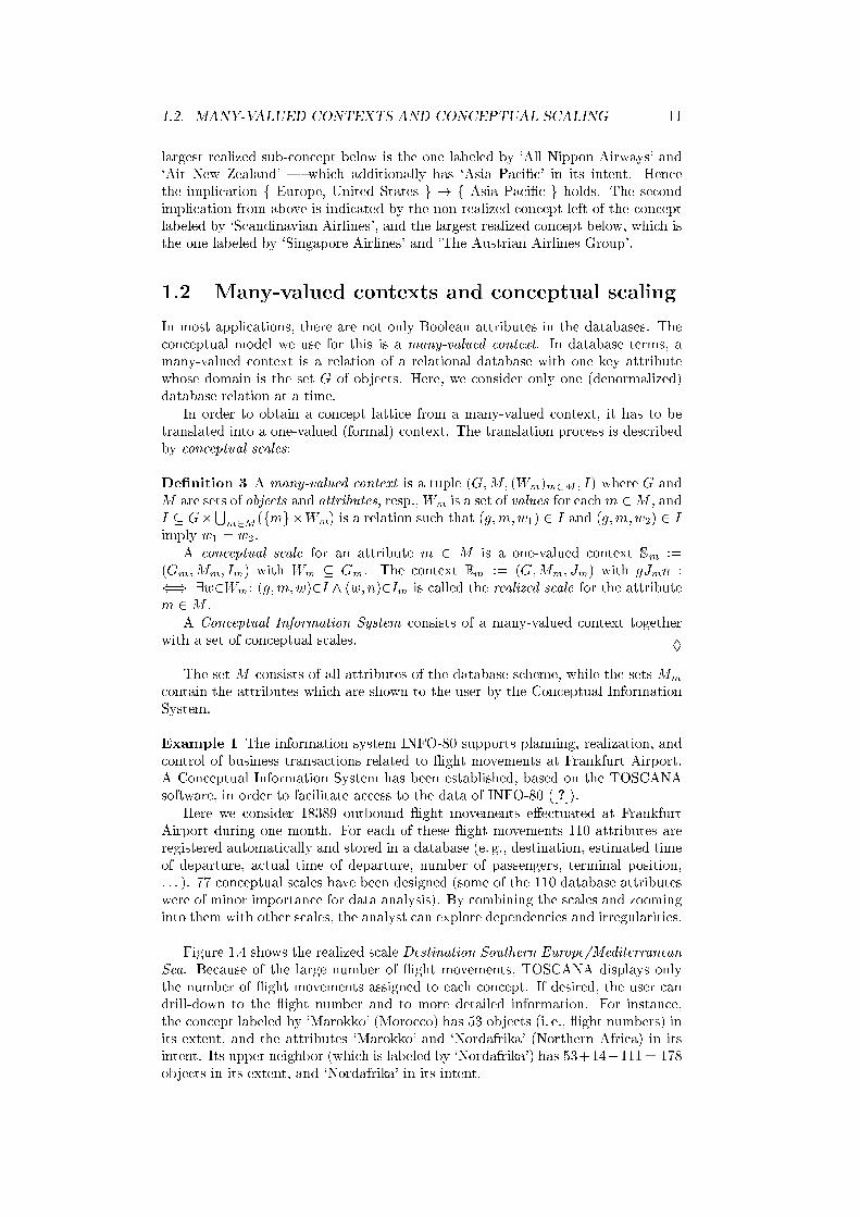
1.2 Many-valued contexts and conceptual scaling
In most applications, there are not only Boolean attributes in the databases. The
conceptual model we use for this is a many-valued context. In database terms, a
many-valued context is a relation of a relational database with one key attribute
whose domain is the set G of objects. Here, we consider only one (denormalized)
database relation at a time.
In order to obtain a concept lattice from a many-valued context, it has to be
translated into a one-valued (formal) context. The translation process is described
by conceptual scales:
De�nition 3 A many-valued context is a tuple (G;M; (Wm)m2M ; I) where G and
M are sets of objects and attributes, resp.,Wm is a set of values for eachm 2M , and
I � G�Sm2M
(fmg�Wm) is a relation such that (g;m;w1) 2 I and (g;m;w2) 2 I
imply w1 = w2.
A conceptual scale for an attribute m 2 M is a one-valued context Sm :=
(Gm;Mm; Im) with Wm � Gm. The context Rm := (G;Mm; Jm) with gJmn :
() 9w2Wm: (g;m;w)2I ^ (w; n)2Im is called the realized scale for the attribute
m 2M .
A Conceptual Information System consists of a many-valued context together
with a set of conceptual scales. �
The set M consists of all attributes of the database scheme, while the sets Mm
contain the attributes which are shown to the user by the Conceptual Information
System.
Example 1 The information system INFO-80 supports planning, realization, and
control of business transactions related to ight movements at Frankfurt Airport.
A Conceptual Information System has been established, based on the TOSCANA
software, in order to facilitate access to the data of INFO-80 ([?]).
Here we consider 18389 outbound ight movements e�ectuated at Frankfurt
Airport during one month. For each of these ight movements 110 attributes are
registered automatically and stored in a database (e. g., destination, estimated time
of departure, actual time of departure, number of passengers, terminal position,
. . . ). 77 conceptual scales have been designed (some of the 110 database attributes
were of minor importance for data analysis). By combining the scales and zooming
into them with other scales, the analyst can explore dependencies and irregularities.
Figure 1.4 shows the realized scale Destination Southern Europe/MediterraneanSea. Because of the large number of ight movements, TOSCANA displays only
the number of ight movements assigned to each concept. If desired, the user can
drill-down to the ight number and to more detailed information. For instance,
the concept labeled by `Marokko' (Morocco) has 53 objects (i. e., ight numbers) in
its extent, and the attributes `Marokko' and `Nordafrika' (Northern Africa) in its
intent. Its upper neighbor (which is labeled by `Nordafrika') has 53+14+111 = 178
objects in its extent, and `Nordafrika' in its intent.

12 CHAPTER 1. FORMAL CONCEPT ANALYSIS IN A NUTSHELL
SpanienPortugal MaltaItalien
Nordafrika
TunesienMarokko
Algerien
Nicht aus diesem Gebiet
985251 701022 11153 14 16433
Figure 1.4: Realized scale Destination Southern Europe/Mediterranean Sea
Halle A Halle B Halle C Halle Mitte Terminal 2 Vorfeld V3
sonst. Angaben
keine unbekannte
keine AngabeT1T2VWG
M
18939834514148551124
46045
2503
242578
2940
2790150
497
48116
1635
1415
4
216
5316
180
12693867
1942
177
1918
4106
10371342306124
460
45
4106
10371342306124460 45
Figure 1.5: Nested line diagram of the scales Position of Baggage Conveyor and
Position of Aircraft
For analyzing how objects are distributed over two di�erent scales, one can
combine the two conceptual scales. The result of combining the two conceptual
scales Position of Baggage Conveyor and Position of Aircraft is displayed in the
nested line diagram in Figure 1.5.
Each of the 17 lines of the outer scale represents seven parallel lines linking
corresponding concepts of the inner scale. The concept lattice we are interested in
is embedded in this direct product. The embedding is indicated by the bold circles.

1.2. MANY-VALUED CONTEXTS AND CONCEPTUAL SCALING 13
Again, each non-realized concept (i. e., the empty circles) indicates an implication.
For example, the leftmost circle in the leftmost ellipse has the attribute `Halle A'
(hall A) and `G' (general aviation, i. e., private airplanes) in its intent. These two
attributes form the premise of the implication. The conclusion of the implication
is given by the intent of the largest realized concept below. In this case, it is the
bottom concept which has all attributes in its extent. Hence hall A as position
of the baggage conveyor and the general aviation apron as position of the aircraft
implies everything else. This means that the premise is not realized by any object.
There are no general aviation aircraft with a baggage conveyor assigned at hall A.
There are concepts in the nested line diagram which are expected to be non-realized
as well. For instance, an aircraft at Terminal 1 should not have a baggage conveyor
assigned at Terminal 2. But in the diagram, we see that the concept with these
two attributes is realized. There are 180 ight movements having the attribute
`Terminal 2' of the outer scale and the attribute `T1' of the inner scale.
We can detect some more unnormal combinations. There are four aircraft that
docked at Terminal 2, while their assigned baggage conveyors are at Terminal 1. To
seven aircraft at Terminal 2 and 17 aircraft at Terminal 1, conveyors on the `Vorfeld
V3' (Apron V3) were assigned. In all these cases, one can drill down to the original
data by clicking on the number to obtain the ight movement numbers, which in
turn lead to the data sets stored in the INFO-80 system.
The knowledge that the combinations are unnormal, is not coded explicitly in
INFO-80, but is only implicitly present as expert knowledge. Since these combina-
tions happen at the airport, they cannot be forbidden by database constraints. But
once such con icts are discovered, one can implement an alarm which informs the
operator of the baggage transportation system about such cases.
If there are too many scales involved in the knowledge discovery process, then
zooming into the outer scale reduces the size of the displayed diagram. For instance,
by zooming into the concept labeled by `Terminal 2' in Fig. 1.5, we obtain the
diagram of the conceptual scale Position of Aircraft, but with the objects being
restricted to those ight movements where the assigned baggage conveyor is at
Terminal 2. Then one can continue the exploration by adding a new conceptual scale
on the inner level. This interactive human-centered knowledge discovery process is
described in detail in [?].
This section gave a short introduction to the core notions of FCA. We will discuss
them (and more advanced topics) in more detail in the remainder of this book.

14 CHAPTER 1. FORMAL CONCEPT ANALYSIS IN A NUTSHELL

Part I
Contexts, Concepts, and
Concept Lattices
15


Chapter 2
Concept lattices
Formal Concept Analysis studies how objects can be hierarchically grouped togetheraccording to their common attributes. One of the aspects of FCA thus is attributelogic, the study of possible attribute combinations. Most of the time, this will be
very elementary. Those with a background in Mathematical Logic might say that
attribute logic is just Propositional Calculus, and thus Boolean Logic, or even a
fragment of this. Historically, the name Propositional Logic is misleading: Boole
himself used the intuition of attributes (\signs") rather than of propositions. So in
fact, attribute logic goes back to Boole.
But our style is di�erent from that of logicians. Our logic is contextual, whichmeans that we are interested in the logical structure of concrete data (of the context).Of course, the general rules of mathematical logic are important for this and will
be utilized.
2.1 Basic notions
2.1.1 Formal contexts and cross tables
De�nition 4 A Formal Context (G;M; I) consists of two sets G and M and of
a binary relation I � G �M . The elements of G are called the objects, those of
M the attributes of (G;M; I). If g 2 G and m 2 M are in relation I , we write
(g;m) 2I or g I M and read this as \object g has attribute M". �
The simplest format for writing down a formal context is a cross table: we write
a rectangular table with one row for each object and one column for each attribute,
having a cross in the intersection of row g with column m i� (g;m) 2 I . The
simplest data type for computer storage is that of a bit matrix1.
Note that the de�nition of a formal context is very general. There are no restric-
tions about the nature of objects and attributes. We may consider physical objects,
or persons, numbers, processes, structures, etc., etc., virtually everything. Any-
thing that is a set in the mathematical sense may be taken as the set of objects or
of attributes of some formal context. We may interchange the role of objects and at-
tributes: if (G;M; I) is a formal context, then so is the dual context (M;G; I�1)
(with (m; g) 2I�1: () (g;m) 2I). It is also not necessary that G and M are
disjoint, they need not even be di�erent.
On the other hand, the de�nition is rather restrictive when applied to real world
phenomena. Language phrases like \all human beings" or \all chairs" do not denote
1It is not easy to say which is the most eÆcient data type for formal contexts. This depends,
of course, on the operations we want to perform with formal contexts. The most important ones
are the derivation operators, to be de�ned in the next subsection.
17
18 CHAPTER 2. CONCEPT LATTICES
sets in our sense. There is no \set of all chairs", because the decision if something is
a chair is not a matter of fact but a matter of subjective interpretation. The notion
of \formal concept" which we shall base on the de�nition of \formal context" is
much, much narrower than what is commonly understood as a concept of human
cognition. The step from \context" to \formal context" is quite an incisive one.
It is the step from \real world" to \data". Later on, when we get tired of saying
\formal concepts of a formal context", we will sometimes omit the word \formal".
But we should keep in mind that it makes a big di�erence.
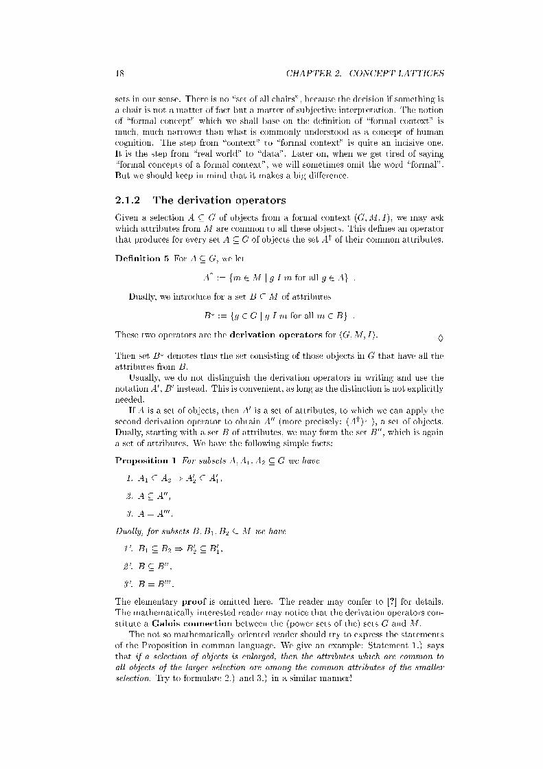
2.1.2 The derivation operators
Given a selection A � G of objects from a formal context (G;M; I), we may ask
which attributes from M are common to all these objects. This de�nes an operator
that produces for every set A � G of objects the set A" of their common attributes.
De�nition 5 For A � G, we let
A" := fm 2M j g I m for all g 2 Ag :
Dually, we introduce for a set B �M of attributes
B# := fg 2 G j g I m for all m 2 Bg :
These two operators are the derivation operators for (G;M; I). �
Then set B# denotes thus the set consisting of those objects in G that have all the
attributes from B.
Usually, we do not distinguish the derivation operators in writing and use the
notationA0, B0 instead. This is convenient, as long as the distinction is not explicitly
needed.
If A is a set of objects, then A0 is a set of attributes, to which we can apply the
second derivation operator to obtain A00 (more precisely: (A")# ), a set of objects.
Dually, starting with a set B of attributes, we may form the set B00, which is again
a set of attributes. We have the following simple facts:
Proposition 1 For subsets A;A1; A2 � G we have
1. A1 � A2 ) A02 � A0
1,
2. A � A00,
3. A = A000.
Dually, for subsets B;B1; B2 �M we have
1'. B1 � B2 ) B02 � B0
1,
2'. B � B00,
3'. B = B000.
The elementary proof is omitted here. The reader may confer to [?] for details.
The mathematically interested reader may notice that the derivation operators con-
stitute a Galois connection between the (power sets of the) sets G and M .
The not so mathematically oriented reader should try to express the statements
of the Proposition in comman language. We give an example: Statement 1.) says
that if a selection of objects is enlarged, then the attributes which are common toall objects of the larger selection are among the common attributes of the smallerselection. Try to formulate 2.) and 3.) in a similar manner!
2.1. BASIC NOTIONS 19
2.1.3 Formal concepts, extent and intent
In what follows, (G;M; I) always denotes a formal context.
De�nition 6 (A;B) is a formal concept of (G;M; I) i�
A � G; B �M; A0 = B; and A = B0:
The set A is called the extent of the formal concept (A;B), and the set B is called
its intent. �
According to this de�nition, a formal concept has two parts: its extent and its
intent. This follows an old tradition in philosophical concept logic, as expressed
in the Logic of Port Royal, 1654 [?], and in the International Standard ISO704
(translation of the German Standard DIN 2330).
The description of a concept by extent and intent is redundant, because each
of the two parts determines the other (since B = A0 and A = B0). But for many
reasons this redundant description is very convenient.
When a formal context is written as a cross table, then every formal concept
(A;B) corresponds to a (�lled) rectangular subtable, with row set A and column
set B. To make this more precise, note that in the de�nition of a formal context
there is no order on the sets G or M . Permuting the rows or the columns of a cross
table therefore does not change the formal context it represents. A rectangularsubtable may, in this sense, omit some rows or columns; it must be rectangular
after an appropriate rearrangement of the rows and the columns. It is then easy to
characterize the rectangular subtables that correspond to formal contexts: they are
full of crosses and maximal with respect to this property:
Lemma 1 (A;B) is a formal concept of (G,M,I)i� A � G, B �M , and A and Bare each maximal (with respect to set inclusion) with the property A�B � I.
A formal context may have many formal concepts. In fact, it is not diÆcult to
come up with examples where the number of formal concepts is exponential in the
size of the formal context. The set of all formal concepts of (G;M; I) is denoted
B(G;M; I):
Later on we shall discuss an algorithm to compute all formal concepts of a given
formal context.
2.1.4 Conceptual hierarchy
Formal concepts can be (partially) ordered in a natural way. Again, the de�ni-
tion is inspired by the way we usually order concepts in a subconcept{superconcepthierarchy: \Pig" is a subconcept of \mammal", because every pig is a mammal.
Transferring this to formal concepts, the natural de�nition is as follows:
De�nition 7 Let (A1; B1) and (A2; B2) be formal concepts of (G;M; I). We say
that (A1; B1) is a subconcept of (A2; B2) (and, equivalently, that (A2; B2) is a
superconcept of (A1; B1) i� A1 � A2. We use the �-sign to express this relation
and thus have
(A1; B1) � (A2; B2) :() A1 � A2:
The set of all formal concepts of (G;M; I), ordered by this relation, is denoted
B(G;M; I)
and is called the concept lattice of the formal context (G;M; I). �

20 CHAPTER 2. CONCEPT LATTICES
This de�nition is natural, but irritatingly asymmetric. What about the intents?
Well, a look at Proposition 1 shows that for concepts (A1; B1) and (A2; B2)
A1 � A2 is equivalent to B2 � B1:
Therefore
(A1; B1) � (A2; B2) :() A1 � A2 (() B2 � B1):
The concept lattice of a formal context is a partially ordered set:
De�nition 8 A partially ordered set is a pair (P;�) where P is a set, and � is a
binary relation on P (i. e.,� is a subset of P � P ) which is
1. re exive (x � x for all x 2 P ),
2. anti-symmetric (x � y ^ x 6= y ) :y � x for all x 2 P ),
3. and transitive (x � y ^ y � z ) x � z for all x; y; z 2 P ),
x � y stands for y �, and x < y for x � y with x 6= y. �
Beside concept lattices, partially ordered sets appear frequently in Mathematics
and Computer Science. We provide some examples.
Example 2 � Every tree is a partially ordered set.
� The set R of all reel numbers together with the ordinary �{relation.� On any set M , the equality = is also a (trivial) order relation.
� For a setM , the powersetP(M) with set inclusion� is also a partially ordered
set.
� The set N of all natural numbers with the divides{relation j.Observe that we do not assume a total order, which would require the additional
condition x � y or y � x for x; y 2 P . Observe also that partially ordered sets
allow for `multiple inheritance', as the two last examples show.
Concept lattices have additional properties beside being partially ordered sets,
that it why we call them `lattices'. This will be the topic of the next section.
2.2 The algebra of concepts
2.2.1 Reading a concept lattice diagram
The concept lattice of (G;M; I) is the set of all formal concepts of (G;M; I), or-
dered by the subconcept{superconcept order. Ordered sets of moderate size can
conveniently be displayed as order diagrams. We explain how to read a concept
lattice diagram by means of an example given in Figure 2.1. Later on we will discuss
how to draw such diagrams.
Figure 2.1 refers to the following situation: Think of two squares, of equal size,
that are drawn on paper. There are di�erent ways to arrange two squares: they
may be disjoint (= have no point in common), may overlap (= have a common
interior point), may share a vertex, an edge or a line segment of the boundary (of
length > 0), they may be parallel or not.
Figure 2.1 shows a concept lattice unfolding these possibilities. It consists of
twelve formal concepts, these being represented by the twelve small circles in the

2.2. THE ALGEBRA OF CONCEPTS 21
common vertexparallel
commonsegment
common edge
overlap
disjoint
Figure 2.1: A concept lattice diagram. The objects are pairs of unit squares. The
attributes describe their mutual position. See also Figure 6.6 (p. 107).
diagram. The names of the six attributes are given. Each name is attached to one
of the formal concepts and is written slightly above the respective circle. The ten
objects are represented by little pictures; each showing a pair of unit squares. Again,
each object is attached to exactly one formal concept; the picture representing the
object is drawn slightly below the circle representing the object concept.
Some of the circles are connected by edges. These express the concept order.
With the help of the edges we can read from the diagram which concepts are sub-
concepts of which other concepts, and which objects have which attributes. To do
so, one has to follow ascending paths in the diagram.
For example, consider the object . From the corresponding circle we can
reach, via ascending paths, four attributes: \common edge", \common segment",
\common vertex", and \parallel". does in fact have these properties, and
does not have the other ones: the two squares are neither \disjoint" nor do they
\overlap".
Similarly, we can �nd those objects that have a given attribute by following all
descending paths starting at the attribute concept. For example, to �nd all objects
which \overlap", we start at the attribute concept labeled \overlap" and follow the
edges downward. We can reach three objects (namely , , and , the
latter symbolizing two squares at the same position). Note that we cannot reach
, because only at concept nodes it is allows to make a turn.
With the same method, we can read the intent and the extent of every formal
concept in the diagram. For example, consider the concept circle labeled . Its
extent consists of all objects that can be reached from that circle on an descending
path. The extent therefore is f ; g. Similarly, we �nd by an inspection of
the ascending paths that the intent of this formal concept is foverlap; parallelg.The diagram contains all necessary information. We can read o� the objects,

22 CHAPTER 2. CONCEPT LATTICES
the attributes, and the incidence relation I . Thus we can perfectly reconstruct the
formal context from the diagram (\the original data").2 Moreover, for each formal
concept we can easily determine its extent and intent from the diagram.
So in a certain sense, concept lattice diagrams are perfect. But there are, of
course, limitations. Take another look at Figure 2.1. Is it correct? Is it complete?The answer is that, since a concept lattice faithfully unfolds the formal context, the
information displayed in the lattice diagram can be only as correct and complete
as the formal context is. In our speci�c example it is easy to check that the given
examples in fact do have the properties as indicated. But a more diÆcult problem
is if our selection of objects is representative. Are there possibilities to combine two
squares, that lead to an attribute combination not occurring in our sample?
We shall come back to that question later.
2.2.2 Supremum and in�mum
Can we compute with formal concepts? Yes, we can. The concept operations are
however quite di�erent from addition and multiplication of numbers. They resemble
more of the operations greatest common divisor and least common multiple, that weknow from integers.
De�nition 9 Let (M;�) be a partially ordered set, and A be a subset of M . A
lower bound of A is an element s of M with s � a, for all a 2 A. An upper
bound of A is de�ned dually. If there exists a largest element in the set of all
lower bounds of A, then it is called the in�mum (or join) of A. It is denoted
inf A orVA. The supremum (or meet) of A (sup A,
WA) is de�ned dually. For
A = fx; yg, we write also x ^ y for their in�mun, and x _ y for their supremum. �
Similarly as for arbitrary sums we use the symbolP
instead of +, we use the
large symbolsW
andV
for arbitrary suprema and in�ma.
Lemma 2 For any two formal concepts (A1; B1) and (A2; B2) of some formal con-text we obtain
� the in�mum (greatest common subconcept) of (A1; B1) and (A2; B2) as
(A1; B1) ^ (A2; B2) := (A1 \ A2; (B1 [B2)00);
� the supremum (least common superconcept) of (A1; B1) and (A2; B2) as
(A1; B1) _ (A2; B2) := ((A1 [ A2)00; B1 \ B2):
It is not diÆcult to prove (Exercise 3) that what is suggested by this de�nition
is in fact true: (A1; B1)^ (A2; B2) is in fact a formal concept (of the same context),
(A1; B1) ^ (A2; B2) is a subconcept of both (A1; B1) and (A2; B2), and any other
common subconcept of (A1; B1) and (A2; B2) is also a subconcept of (A1; B1) ^(A2; B2). Similarly, (A1; B1) _ (A2; B2) is a formal concept, it is a superconcept of
(A1; B1) and of (A2; B2), and it is a subconcept of any common superconcept of
these two formal concepts.
With some practice, one can read o� in�ma and suprema from the lattice dia-
gram. Choose any two concepts from Figure 2.1 and follow the descending paths
from the corresponding nodes in the diagram. There is always a highest point where
these paths meet, that is, a highest concept that is below both, namely, the in�-
mum. Any other concept below both can be reached from the highest one on a
2This reconstruction is assured by the Basic Theorem given below.

2.2. THE ALGEBRA OF CONCEPTS 23
descending path. Similarly, for any two formal concepts there is always a lowest
node (the supremum of the two), that can be reached from both concepts via as-
cending paths. And any common superconcept of the two is on an ascending path
from their supremum.
2.2.3 Complete lattices
The operations for computing with formal concepts, in�mum and supremum, are
not as weird as one might suspect. In fact, we obtain with each concept lattice
an algebraic structure called a \lattice", and such structures occur frequently in
mathematics and computer science. \Lattice theory" is an active �eld of research in
mathematics. A lattice is an algebraic structure with two operations (called \meet"
and \join" or \in�mum" and \supremum") that satisfy certain natural conditions:3
De�nition 10 A partially ordered set V := (V;�) is a lattice, if their exists, forevery pair of elements x; y 2 V , their in�mum x ^ y and their supremum x _ y. �
We shall not discuss the algebraic theory of lattices in this lecture. Many uni-
versities o�er courses in lattice theory, and there are excellent textbooks.4
Concept lattices have an additional nice property: they are complete lattices.
This means that the operations of in�mum and supremum do not only work for
an input consisting of two elements, but for arbitrary many. In other words: each
collection of formal concepts has a greatest common subconcept and a least com-
mon superconcept. This is even true for in�nite sets of concepts. The operations
\in�mum" and \supremum" are not necessarily binary, they work for any input
size.
De�nition 11 A partially ordered set V := (V;�) is a complete lattice, if for
every set A � V exist its in�mumVV and its supremum
WA. �
The de�nition requests the existence of in�mum and supremum for every set A,
hence also for the empty set A := ;. Following the de�nition, we obtain thatV ;
has to be the (unique) largest element of the lattice. It is denoted by 1V. Dually,W ; has to be the smallest element of the lattice; it is denoted by 0V.
The arbitrary arity of in�mum and supremum is very useful, but will make
essentially no di�erence for our considerations, because we shall mainly be concerned
with �nite formal contexts and �nite concept lattices. Well, this is not completely
true. In fact, although the concept lattice in Figure 2.1 is �nite, its ten objects are
representatives for all possibilities to combine two unit squares. Of course, there
are in�nitely many such possibilities. It is true that we shall consider �nite concept
lattices, but our examples may be taken from an in�nite reservoir.
2.2.4 The Basic Theorem
We give now a mathematically precise formulation of the algebraic properties of
concept lattices. The theorem below is not diÆcult, but basic for many other
results. Its formulation contains some technical terms that we have not mentioned
so far.
To understand the notion of a \supremum-dense" set, think of the positive
integers with the least common multiple (LCM) in the role of the supremum op-
eration. Some numbers can be written as a LCM of other integers. For example,
3Unfortunately, the word \lattice" is used with di�erent meanings in mathematics. It also
refers to generalized grids.4An introduction to lattices and order by B. Davey and H. Priestley is particularly popular
among CS students.

24 CHAPTER 2. CONCEPT LATTICES
12 = LCMf3; 4g. Therefore, 12 is called LCM-reducible. Prime numbers cannot
be written as an LCM of other numbers. Therefore, prime numbers are LCM-
irreducible. But prime numbers are not the only LCM-irreducible numbers. For
example, 25 is not the least common multiple of other numbers, and thus is LCM-
irreducible. It is easy to see that the LCM-irreducible integers are precisely the
prime powers5. The set of prime powers is LCM-dense, which means that every
positive integer can be written as a LCM of prime powers. Any larger set, that is,
any set containing all prime powers, is also LCM-dense, of course.
There are no GCD-irreducible numbers. Every positive integer can be written
as the GCD of other numbers. But there are GCD-dense sets of numbers. For
example, the set of all integers greater than 1000 is GCD-dense.
In a complete lattice, an element is called supremum-irreducible if it cannot
be written as an supremum of other elements, and in�mum-irreducible if it can
not be expressed as an in�mum of other elements. It is very easy to locate the
irreducible elements in a diagram of a �nite lattice: the supremum-irreducible el-
ements are precisely those from which there is exactly one edge going downward.
An element is in�mum-irreducible if and only if it is the start of exactly one up-
ward edge. In Figure 2.1 there are precisely nine supremum-irreducible concepts
and precisely �ve in�mum-irreducible concepts. Exactly four concepts have both
properties, they are doubly irreducible.
A set of elements of a complete lattice is called supremum-dense, if every
lattice element is a supremum of elements from this set. Dually, a set is called
in�mum-dense, if the in�ma that can be computed from this set exhaust all
lattice elements.
De�nition 12 Two complete lattices V and W are isomorphic (V �= W ), if there
exists a bijective mapping ':V ! W with x � y () '(x) � '(y). The mapping
' is then called lattice isomorphism between V and W . �
Example 3 The lattice (f1; 2; 3; 5; 6; 10; 12; 15; 30g; j) is isomorphic to the powerset
(P(f2; 3; 5g);�) with the isomorphism ': f1; 2; 3; 5; 6; 10; 12; 15; 30g ! P(f2; 3; 5g)with '(x) := fy 2 f2; 3; 5g j y divides xg.
Now we have de�ned all the terminology necessary for stating the main theorem
of Formal Concept Analysis.
Theorem 1 (The basic theorem of Formal Concept Analysis.) The conceptlattice of any formal context (G;M; I) is a complete lattice. For an arbitrary setf(Ai; Bi) j i 2 Ig � B(G;M; I) of formal concepts, the supremum is given by
_i2I
(Ai; Bi) =
([i2I
Ai)00;\i2I
Bi
!
and the in�mum is given by
^i2I
(Ai; Bi) =
\i2I
Ai; ([i2I
Bi)00
!:
A complete lattice L is isomorphic to B(G;M; I) i� there are mappings ~ : G! L
and ~� : M ! L such that ~ (G) is supremum-dense and ~�(M) is in�mum-dense inL, and
g I m () ~ (g) � ~�(m):
In particular, L �= B(L;L;�):5The number 1 requires special treatment. We shall not go into this.

2.2. THE ALGEBRA OF CONCEPTS 25
The theorem is less complicated as it �rst may seem. We give some explanations
below. Readers in a hurry may skip these and continue with the next section.
The �rst part of the theorem gives the precise formulation for in�mum and
supremum of arbitrary sets of formal concepts. The second part of the theorem
gives (among other information) an answer to the question if concept lattices have
any special properties. The answer is \no": every complete lattice is (isomorphic
to) a concept lattice. This means that for every complete lattice we must be able
to �nd a set G of objects, a set M of attributes and a suitable relation I , such that
the given lattice is isomorphic to B(G;M; I). The theorem does not only say how
this can be done, it describes in fact all possibilities to achieve this.
In Figure 2.1, every object is attached to a unique concept, the corresponding
object concept. Similarly for each attribute there corresponds an attribute concept.These can be de�ned as follows:
De�nition 13 Let (G;M; I) be some formal context. Then
� for each object g 2 G the corresponding object concept is
g := (fgg00; fgg0);
� and for each attribute m 2M the attribute concept is given by
�m := (fmg0; fmg00):
The set of all object concepts of (G;M; I) is denoted G, the set of all attribute
concepts is �M . �
Using De�nition 6 and Proposition 1 it is easy to check that these expressions in
fact de�ne formal concepts of (G;M; I).
We have that g � (A;B) () g 2 A. A look at the �rst part of the Basic
Theorem shows that each formal concept is the supremum of all the object concepts
below it (Exercise 4). Therefore, the set G of all object concepts is supremum-
dense. Dually, the attribute concepts form am in�mum dense set in B(G;M; I).
The Basic Theorem says that, conversely, any supremum-dense set in a complete
lattice L can be taken as the set of objects and any in�mum-dense set be taken as
a set of attributes for a formal context with concept lattice isomorphic to L.
We conclude with a simple observation that often helps to �nd errors in con-
cept lattice diagrams. The fact that the object concepts form an supremum-dense
set implies that every supremum-irreducible concept must be an object concept
(the converse is not true). Dually, every in�mum-irreducible concept must be an
attribute concept. This yields the following rule for concept lattice diagrams:
Proposition 2 Given a formal context (G;M; I) and a �nite order diagram, labeledby the objects from G and the attributes from M . For g 2 G let ~ (g) denote theelement of the diagram that is labeled with g, and let ~�(m) denote the element labeledwith m. Then the given diagram is a correctly labeled diagram of B(G;M; I) if andonly if it ful�lls the following conditions:
1. The diagram is a correct lattice diagram,
2. every supremum-irreducible element is labeled by some object,
3. every in�mum-irreducible element is labeled by some attribute,
4. g I m () ~ (g) � ~�(m).

26 CHAPTER 2. CONCEPT LATTICES
2.2.5 The duality principle
The de�nitions of lattices and complete lattices are self-dual: If (V;�) is a (com-
plete) lattice, then (V;�)d := (V;�) is also a (complete) lattice. If a theorem holds
for a (complete) lattice, then the `dual theorem' also holds, i. e., the theorem where
all occurences of �;_;^;W;V;0V;1V etc. are replaced by �;^;_;V;W;1V;0V,resp.
For concept lattices, their dual can be obtained by \permuting" the formal
context:
Lemma 3 Let (G;M; I) be a formal context. Then (B((G;M; I)))d �= B(M;G; I�1),where I�1 := f(m; g) 2M �G j (g:m) 2 Ig.
2.3 Computing and drawing concept lattices
2.3.1 Computing all concepts
There are several algorithms that help drawing concept lattices. We shall discuss
some of them below. But we �nd it instructive to start by some small examples
that can be drawn by hand. For computing concept lattices, we will investigate a
fast algorithm later. We start with a naive method, and proceed then to a method
which is suitable for manual computation.
In principle, it is not diÆcult to �nd all the concepts of a formal context. The
following proposition summarizes the naive possibilities of generating all concepts:
Lemma 4 Each concept of a context (G;M; I) has the form (X 00; X 0) for somesubset X � G and the form (Y 0; Y 00) for some subset Y �M . Conversely, all suchpairs are concepts.
Every extent is the intersection of attribute extents and every intent is the in-tersection of object intents.
The �rst part of the lemma suggests the following, �rst algorithm for computing
all concepts:
1. B(G;M; I) := ;;
2. For all subsets X of G, add (X 00; X 0) to B(G;M; I);
However, this is rather ineÆcient, and not practicable even for relatively small
contexts. The second part of the proposition at least yields the possibility to cal-
culate the concepts of a small context by hand.
The following method is more eÆcient, and is recommended for computations
by hand. It is based on the following observations:
1. It suÆces to determine all concept extents [or all concept intents] of (G;M; I),
since we can always determine the other part of a formal concept with the help of the
derivation operators.
2. The intersection of arbitrary many extents is an extent [and the intersection
of arbitrary intents is an intent].
This follows easily from the formulae given in the Basic Theorem. By the way: a convention
that may seem absurd on the �rst glance allows to include in \arbitrary many" also the
case \zero". The convention says that the intersection of zero intents equals M and the
intersection of zero extents equals G.
2.3. COMPUTING AND DRAWING CONCEPT LATTICES 27
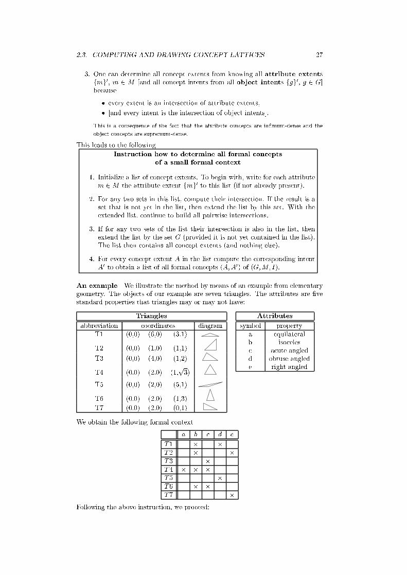
3. One can determine all concept extents from knowing all attribute extents
fmg0, m 2 M [and all concept intents from all object intents fgg0, g 2 G]
because
� every extent is an intersection of attribute extents,
� [and every intent is the intersection of object intents].
This is a consequence of the fact that the attribute concepts are in�mum-dense and the
object concepts are supremum-dense.
This leads to the following
Instruction how to determine all formal concepts
of a small formal context
1. Initialize a list of concept extents. To begin with, write for each attribute
m 2M the attribute extent fmg0 to this list (if not already present).
2. For any two sets in this list, compute their intersection. If the result is a
set that is not yet in the list, then extend the list by this set. With the
extended list, continue to build all pairwise intersections.
3. If for any two sets of the list their intersection is also in the list, then
extend the list by the set G (provided it is not yet contained in the list).
The list then contains all concept extents (and nothing else).
4. For every concept extent A in the list compute the corresponding intent
A0 to obtain a list of all formal concepts (A;A0) of (G;M; I).
An example We illustrate the method by means of an example from elementary
geometry. The objects of our example are seven triangles. The attributes are �ve
standard properties that triangles may or may not have:
Triangles
abbreviation coordinates diagram
T1 (0,0) (6,0) (3,1)
T2 (0,0) (1,0) (1,1)
T3 (0,0) (4,0) (1,2)
T4 (0,0) (2,0) (1,p3)
T5 (0,0) (2,0) (5,1)
T6 (0,0) (2,0) (1,3)
T7 (0,0) (2,0) (0,1)
Attributes
symbol property
a equilateral
b isoceles
c acute angled
d obtuse angled
e right angled
We obtain the following formal context
a b c d e
T1 � �T2 � �T3 �T4 � � �T5 �T6 � �T7 �
Following the above instruction, we proceed:

28 CHAPTER 2. CONCEPT LATTICES
1. Write the attribute extents to a list.
No. extent found as
e1 := fT4g fag0e2 := fT1; T2; T4; T6g fbg0e3 := fT3; T4; T6g fcg0e4 := fT1; T5g fdg0e5 := fT2; T7g feg0
2. Compute all pairwise intersections, and
3. add GNo. extent found as
e1 := fT4g fag0e2 := fT1; T2; T4; T6g fbg0e3 := fT3; T4; T6g fcg0e4 := fT1; T5g fdg0e5 := fT2; T7g feg0e6 := � e1 \ e4e7 := fT4; T6g e2 \ e3e8 := fT1g e2 \ e4e9 := fT2g e2 \ e5e10 := fT1; T2; T3; T4; T5; T6; T7g step 3
4. Compute the intents
Concept No. (extent ; intent)
1 (fT4g ; fa; b; cg)2 (fT1; T2; T4; T6g ; fbg)3 (fT3; T4; T6g ; fcg)4 (fT1; T5g ; fdg)5 (fT2; T7g ; feg)6 (� ; fa; b; c; d; eg)7 (fT4; T6g ; fb; cg)8 (fT1g ; fb; dg)9 (fT2g ; fb; eg)10 (fT1; T2; T3; T4; T5; T6; T7g ; �)
We have now computed all ten formal concepts of the triangles{context. The last
step can be skipped if we are not interested in an explicit list of all concepts, but
just in computing a line diagram.
2.3.2 Drawing concept lattices
Based on one of the lists 3. or 4., we can start to draw a diagram. Before doing so,
we give two simple de�nitions.
De�nition 14 Let (A1; B1) and (A2; B2) be formal concepts of (G;M; I).
We say that (A1; B1) is a proper subconcept of (A2; B2), if (A1; B1) �(A2; B2) and, in addition, (A1; B1) 6= (A2; B2) holds. As an abbreviation, we write
(A1; B1) < (A2; B2).
We say that (A1; B1) is a lower neighbour of (A2; B2), if (A1; B1) < (A2; B2),
but no formal concept (A;B) of (G;M; I) exists with (A1; B1) < (A;B) < (A2; B2).
The abbreviation for this is (A1; B1) � (A2; B2). �

2.3. COMPUTING AND DRAWING CONCEPT LATTICES 29
Instruction how to draw a line diagram of a small concept lattice
5. Take a sheet of paper and draw a small circle for every formal concept, in
the following manner: a circle for a concept is always positioned higher
than the all circles for its proper subconcepts.
6. Connect each circle with the circles of its lower neighbors.
7. Label with attribute names: attach the attribute m to the circle repre-
senting the concept (fmg0; fmg00).8. Label with object names: attach each object g to the circle representing
the concept (fgg00; fgg0).We follow these instructions.
5. Draw a circle for each of the formal concepts:
6
1
9 8 7
5 2 4 3
10
6. Connect circles with their lower neighbours:
7. Add the attribute names:

30 CHAPTER 2. CONCEPT LATTICES
a
b cde
8. Determine the object concepts
Object g object intent fgg0 No. of concept
T1 fb; dg 8
T2 fb; eg 9
T3 fcg 3
T4 fa; b; cg 1
T5 fdg 4
T6 fb; cg 7
T7 feg 5
and add the object names to the diagram:
a
b cde
T1T2
T3
T4
T5
T6
T7
Ready! Usually it takes some tries before a nice, readable diagram is achieved.
Finally we can make the e�ort to avoid abbreviations and to increase the readability.
The result is shown in Figure 2.2.
2.3.3 Clarifying and reducing a formal context
There are context manipulations that simplify a formal context without changing
the diagram, except for the labellig. It is usually advisable to do these manipulations
�rst, before starting computations.
The simplest operation is clari�cation, which refers to indentifying \equal
rows" of a formal context, and \equal columns" as well. What is meant is that

2.3. COMPUTING AND DRAWING CONCEPT LATTICES 31
equilateral
isoceles
acute angled
obtuse angled
right angled
Figure 2.2: A diagram of the concept lattice of the triangle context.
if a context contains objects g1; g2; : : : with fgig0 = fgjg0 for all i; j, that is, objectswhich have exactly the same attributes, then these can be replaced by a single ob-
ject, the name of which is just the list of names of these objects. The same can be
done for attributes with identical attribute extent.
De�nition 15 We say that a formal context is clari�ed if no two of its object
intents are equal and no two of its attribute extents are equal. �
A stronger operation is reduction, which refers to omitting attributes that are
equivalent to combinations of other attributes (and dually for objects). For de�ning
reduction it is convenient to work with a clari�ed context.
De�nition 16 An attribute m of a clari�ed context is called reducible if there is
a set S � M of attributes with fmg0 = S0, otherwise it is irreducible. Reduced
objects are de�ned dually. A formal context is called reduced, if all objects and
all attribues are irreducible. �
fmg0 = S0 means that an object g has the attribute m if and only if it has all the
attributes from S. If we delete the column m from our cross table, no essential
information is lost because we can reconstruct this column from the data contained
in other columns (those of S). Moreover, deleting that column does not change the
number of concepts, nor the concept hierarchy, because fmg0 = S0 implies that m
is in the intent of a concept if and only if S is contained in that intent. The same
is true for reducible objects and concept extents. Deleting a reducible object from
a formal context does not change the structure of the concept lattice.
It is even possible to remove several reducible objects and attributes simultane-
ously from a formal context without any e�ect on the lattice structure, as long as
the number of removed elements is �nite.
De�nition 17 Let (G;M; I) be a �nite context, and let Girr be the set of irre-
ducible objects and Mirr be the set of irreducible attributes of (G;M; I). The
context (Girr ;Mirr; I \ Girr � Mirr) is the reduced context corresponding to
(G;M; I).
For a �nite lattice L let J(L) denote the set of its supremum-irreducible el-
ements and let M(L) denote the set of its in�mum-irreducible elements. Then
(J(L);M(L);�) is the standard context for the lattice L. �

32 CHAPTER 2. CONCEPT LATTICES
Proposition 3 A �nite context and its reduced context have isomorphic conceptlattices. For every �nite lattice L there is (up to isomorphism) exactly one reducedcontext, the concept lattice of which is isomorphic to L, namely its standard context.
2.3.4 Other algorithms for computing concept lattices
The algorithm which we shall use in what follows to generate all formal concepts of a
given formal context can be formulated without referring to concept lattices. It will
be an algorithm to generate all closed sets of a closure system, calledNextclosure.
It can be applied to concept lattices because for each formal context (G;M; I), the
set Ext(G;M; I) of all concept extents is a closure system, as well as the set
Int(G;M; I) of all the concept intents of (G;M; I).
||{(to be written)||{
� Titanic
� Nourine
� . . .
2.3.5 Computer programs for concept generation and lattice
drawing
There are several free or conditionally free programs available for concept lat-
tice generation and/or drawing. A well known one, old fashioned but reliable, is
CONIMP (for DOS), available under www.mathematik.tu-darmstadt.de. S. Yev-
tushenko provides the Concept Explorer, which allows for editing formal contexts
and computing their concept lattices. It can be downloaded from http://sourceforge.
net/projects/conexp/. A rather advanced package, invented for applications in
data analysis, is theNavicon Decision Suite byNaviconGmbH. A demo version
is available under www.navicon.de.
2.4 Additive and Nested Line Diagrams
In this section, we discuss possibilities to generate line diagrams both automatically
or by hand. A list of some dozens of concepts may already be quite diÆcult to
survey, and it requires practice to draw good line diagrams of concept lattices with
more than 20 elements.
The best and most versatile form of representation for a concept lattice is a
well drawn line diagram. It is however tedious to draw such a diagram by hand
and one would wish an automatic generation by means of a computer. We know
quite a few algorithms to do this, but none which provides a general satisfactory
solution. It is by no means clear which qualities make up a good diagram. It should
be transparent, easily readable and should facilitate the interpretation of the data
represented. How this can be achieved in each individual case depends however on
the aim of the interpretation and on the structure of the lattice. Simple optimization
criteria (minimization of the number of edge crossings, drawing in layers, etc.) often
bring about results that are unsatisfactory. Nevertheless, automatically generated
diagrams are a great help: they can serve as the starting point for drawing by
hand. Therefore, we will describe simple methods of generating and manipulating
line diagrams by means of a computer.

2.4. ADDITIVE AND NESTED LINE DIAGRAMS 33
2.4.1 Additive line diagrams
We will now explain a method where a computer generates a diagram and o�ers the
possibility of improving it interactively. Programming details are irrelevant in this
context. We will therefore only give a positioning rule which assigns points in
the plane to the elements of a given ordered set (P;�). If a and b are elements of P
with a < b, the point assigned to a must be lower than the point assigned to b (i.e.,
it must have a smaller y-coordinate). This is guaranteed by our method. We will
leave the computation of the edges and the checking for undesired coincidences of
vertices and edges to the program. We do not even guarantee that our positioning
is injective (which of course is necessary for a correct line diagram). This must also
be checked if necessary.
De�nition 18 A set representation of an ordered set (P;�) is an order embed-
ding of (P;�) in the power-set of a set X , i.e., a map
rep : P ! P(X)
with the property
x � y () repx � rep y:
�
An example of a set representation for an arbitrary ordered set (P;�) is the
assignment
X := P; a 7! (a]:
In the case of a concept lattice,
X := G; (A;B) 7! A
is a set representation.
X :=M; (A;B) 7!M nBis another set representation, and both can be combined to
X := G _[M; (A;B) 7! A [ (M nB):
It is suÆcient to limit oneself to the irreducible objects and attributes.
For an additive line diagram of an ordered set (P;�) we need a set represen-
tation rep : P ! P(X) as well as a grid projection
vec : X ! R2 ;
assigning a real vector with a positive y-coordinate to each element of X . By
pos p := n+X
x2repp
vecx
we obtain positioning of the elements of P in the plane. Here, n is a vector which
can be chosen arbitrarily in order to shift the entire diagram. By only allowing
positive y-coordinates for the grid projection we make sure that no element p is
positioned below an element q with q < p.
Every �nite line diagram can be interpreted as an additive diagram with respect
to an appropriate set representation. For concept lattices we usually use the rep-
resentation by means of the irreducible objects and/or attributes. The resulting
diagrams are characterized by a great number of parallel edges, which improves
their readability. Experience shows that the set representation by means of the

34 CHAPTER 2. CONCEPT LATTICES
irreducible attributes is most likely to result in an easily interpretable diagram.
Figure 2.2 for instance was obtaining by selecting the irreducible attributes for the
set representation.
It is particularly easy to manipulate these diagrams: If we change {the set
representation being �xed{ the grid projection for an element x 2 X , this means
that all images of the order �lter fp 2 P j x 2 rep pg are shifted by the same
distance and that all other points remain in the same position. In the case of the set
representation by means of the irreducibles these order �lters are precisely principal
�lters or complements of principal ideals, respectively. This means that we can
manipulate the diagram by shifting principal �lters or principal ideals, respectively,
and leaving all other elements in position.
Even carefully constructed line diagrams loose their readability from a certain
size up, as a rule from around 50 elements up. One gets considerably further with
nested line diagrams which will be introduced next. However, these diagrams do
not only serve to represent larger concept lattices. They o�er the possibility to
visualize how the concept lattice changes if we add further attributes.
2.4.2 Nested line diagrams
Nested line diagrams permit a satisfactory graphical representation of somewhat
larger concept lattices. The basic idea of the nested line diagram consists of clus-
tering parts of an ordinary diagram and replacing bundles of parallel lines between
these parts by one line each. Thus, a nested line diagram consists of ovals, which
contain clusters of the ordinary line diagram and which are connected by lines.
In the simplest case two ovals which are connected by a simple line are congru-
ent. Here, the line indicates that corresponding circles within the ovals are direct
neighbors, resp.
Furthermore, we allow that two ovals connected by a single line do not neces-
sarily have to be congruent, but they may each contain a part of two congruent
�gures. In this case, the two congruent �gures are drawn in the ovals as a \back-
ground structure", and the elements are drawn as bold circles if they are part of the
respective substructures. The line connecting the two boxes then indicates that the
respective pairs of elements of the background shall be connected with each other.
An example is given in Figure 2.3. It is a screenshot of a library information sys-
tem which was set up for the library of the Center on Interdisciplinary Technology
Research of Darmstadt University of Technology.
Nested line diagrams originate from partitions of the set of attributes. The basis
is the following theorem:
Theorem 2 Let (G;M; I) be a context and M =M1 [M2. The map
(A;B) 7! (((B \M1)0; B \M1) ; ((B \M2)
0; B \M2))
is aW-preserving order embedding of B(G;M; I) in the direct product of B(G;M1; I\
G�M1) and B(G;M2; I \G�M2). The component maps
(A;B) 7! ((B \Mi)0; B \Mi)
are surjective on B(G;Mi; I \G�Mi).
Proof If (A;B) is a concept of (G;M; I), then B \Mi is the set of all attributes
common to the objects of A in the context (G;Mi; I \G�Mi), i.e., it is an intent
of this context. Hence the above-mentioned assignment is really a map into the
product. The union of the intents B \M1 and B \M2 again yields B, i.e., the
map is injective. The fact that it is furthermoreW-preserving (and thus an order-
embedding) can again be seen from the concept intents. It remains to be shown

2.4. ADDITIVE AND NESTED LINE DIAGRAMS 35
GeographieDeutschland
America
G e r m a n yImportant Industrial Countries
Europe
Federal Republic*
GDR*
G e r m a n y *Eastern Germany*
834
106
9
9 2
321
4
71
32 2
27
251
56
Forschen für die Zukunft : Wissenschaft Jahrbuch Arbeit und Technik 1991 : Schwe
3
8
145
64
20
36
1
John von Neumann and Norbert Wiener : Fr33
1
68
15
Figure 2.3: Nested line diagram of a library information system
that the component maps are surjective. Let C be an intent of (G;Mi; I \G�Mi).
Then B := CII is an intent of (G;M; I) with B \Mi = C, i.e., the image of the
concept (B0; B) of (G;M; I) under the ith component map is the concept with the
intent C. �
In order to sketch a nested line diagram, we proceed as follows: First of all we
split up the attribute set: M = M1 [M2. This splitting up does not have to be
disjoint. More important for interpretation purposes is the idea that the sets Mi
bear meaning. Now, we draw line diagrams of the subcontexts K i := (G;Mi; I \G�Mi), i 2 f1; 2g and label them with the names of the objects and attributes, as
usual. Then we sketch a nested diagram of the product of the concept latticesB(K i )
as an auxiliary structure. For this purpose we draw a large copy of the diagram
of B(K 1 ), representing the lattice elements not by small circles but by congruent
ovals, which contain each a diagram of B(K 2 ).
By Theorem 2 the concept lattice B(G;M; I) is embedded in this product as aW-semilattice. If a list of the elements of B(G;M; I) is available, we can enter them

36 CHAPTER 2. CONCEPT LATTICES
into the product according to their intents. If not, we enter the object concepts the
intents of which can be read o� directly from the context, and form all suprema.
This at the same time provides us with a further, quite practicable method of
determining a concept lattice by hand: split up the attribute set as appropriate,
determine the (small) concept lattices of the subcontexts, draw their product in form
of a nested line diagram, enter the object concepts and close it against suprema.
This method is particularly advisable in order to arrive at a useful diagram quickly.
2.5 Examples
||{(to be written)||{
2.6 Exercises
1. Give the formal context for the concept lattice shown in Figure 2.1.
2. Give a proof of Proposition 1.
3. Let (A1; B1) and (A2; B2) be formal concepts of a formal context (G;M; I).
Show that the expression `greatest common subconcept' in Lemma 2 is justi-
�ed by showing
(a) (A1; B1) ^ (A2; B2) is a formal concept (of the same context).
(b) (A1; B1) ^ (A2; B2) is a subconcept of both (A1; B1) and (A2; B2).
(c) Any other common subconcept of (A1; B1) and (A2; B2) is also a sub-
concept of (A1; B1) ^ (A2; B2).
4. Show that, in a concept lattice, the set of all object concepts is supremum-
dense. Hint: Show that each formal concept is the supremum of the set of all
its subconcepts which are also object concepts.
5. Let (V;�) be a partially ordered set where every subset A of V has an in�mum.
Show that (V;�) is a complete lattice.
6. Show that every non-empty �nite lattice is a complete lattice.
7. Show that in every lattice the following equivalences hold:
x � y () x ^ y = x () x _ y = y
Remark: From the knowledge about in�ma and suprema of a lattice, we are
thus able to reconstruct its order relation.
8. Prove Lemma 3: For any formal context (G;M; I), the concept lattices (B((G;M; I)))d
and B(M;G; I�1) are isomorphic.
9. Let V and V be two complete lattices, and ':V ! W be a bijective mapping.
Show that ' is an isomorphism of complete lattices if and only if, for all
subsets X of V ,
'�_
X�=_f'(x) j x 2 Xg
and
'�^
X�=^f'(x) j x 2 Xg :