1

Condition based maintenance optimization for wind power generation

systems under continuous monitoring

Zhigang Tiana,

, Tongdan Jinb, Bairong Wu

a, Fangfang Ding

a

a Concordia Institute for Information Systems Engineering, Concordia University, Canada

b Ingram School of Engineering, Texas State University, USA

Abstract

By utilizing condition monitoring information collected from wind turbine components,

condition based maintenance (CBM) strategy can be used to reduce the operation and

maintenance costs of wind power generation systems. The existing CBM methods for wind

power generation systems deal with wind turbine components separately, that is, maintenance

decisions are made on individual components, rather than the whole system. However, a wind

farm generally consists of multiple wind turbines, and each wind turbine has multiple

components including main bearing, gearbox, generator, etc. There are economic dependencies

among wind turbines and their components. That is, once a maintenance team is sent to the wind

farm, it may be more economical to take the opportunity to maintain multiple turbines, and when

a turbine is stopped for maintenance, it may be more cost-effective to simultaneously replace

multiple components which show relatively high risks. In this paper, we develop an optimal

CBM solution to the above-mentioned issues. The proposed maintenance policy is defined by

two failure probability threshold values at the wind turbine level. Based on the condition

monitoring and prognostics information, the failure probability values at the component and the

turbine levels can be calculated, and the optimal CBM decisions can be made accordingly. A

simulation method is developed to evaluate the cost of the CBM policy. A numerical example is

Corresponding author. 1515 Ste-Catherine Street West EV-7.637, Montreal, H3G 2W1, Canada. Tel.: 1-514-848-

2424 ext. 7918; Fax: 1-514-848-3171. Email address: tian@ciise.concordia.ca.

2

provided to illustrate the proposed CBM approach. A comparative study based on commonly

used constant-interval maintenance policy demonstrates the advantage of the proposed CBM

approach in reducing the maintenance cost.

Keywords: condition based maintenance; wind turbine; optimization; simulation; preventive

maintenance; artificial neural network.

1. Introduction

Maintenance management for wind power generation systems aims at reducing the overall

maintenance cost and improving the availability of the systems. Since the operation and

maintenance costs represent a substantial portion of the total life cycle costs of wind power

generation systems [1], reliability and maintenance management of wind turbines have drawn

increasing interests for the reduction of these costs [2-5]. The existing maintenance methods for

wind energy systems can be classified into corrective maintenance, preventive maintenance (PM)

and condition based maintenance (CBM) [6]. PM can be further divided into time-based and

usage-based maintenance depending on the trigger mechanism. In time-based maintenance, the

maintenance activities are routinely carried out based on the predetermined time interval or the

age of the components. If the wind turbine lifetime is measured by usages such as the amount of

energy produced, the maintenance action is triggered once the system has generated a specified

amount of electricity. In many studies, though, the usage-based maintenance can be treated as a

special case of the time-based maintenance in which the time is measured by the usage. Two

challenging issues are always involved in PM: under-maintenance and over-maintenance. The

former occurs when the system performance is not appropriately monitored, resulting in

unexpected failures. For the over-maintenance, we tend to schedule excessive maintenance

activities to prevent the unexpected down events, resulting in the waste of resources.

CBM is an advanced maintenance strategy that is based on performance and/or parameter

monitoring and subsequent actions [7]. Maintenance decision is reached based on condition

monitoring data, such as vibration data, acoustic emission data, oil analysis data and power

3

voltage and current data, which are collected from wind turbine components[8-9] . In [10-12],

Fourier transforms are used as a major signal processing technique for monitoring the wind

turbine health conditions, which turns out to be very promising in dealing with stationary

degradation signals. In reality, signals from wind turbines are often non-stationary as large wind

turbines often operate at variable speeds. The wavelet transform seems more appropriate in

handling non-stationary signals [13]. In [14], a life cycle cost approach is adopted to evaluate the

financial benefit using condition monitoring system, a tool for implementing CBM policy. In

[15] a multi-state Markov decision process is used to estimate the wind turbine degradation

process based on which the optimal maintenance scheme is devised.

By leveraging condition monitoring information, CBM is expected to reduce the operation and

maintenance costs of wind power generation systems. Existing CBM methods for wind power

generation systems deal with wind turbine components separately, that is, maintenance decisions

are made on individual components, rather than the whole system [16]. However, wind farms are

often located in remote areas or off-shore sites. Each wind farm consists of multiple wind

turbines, and each wind turbine has multiple components including main bearing, gearbox,

generator, shafts, etc. Obviously, there are economic dependencies among wind turbines and

their components. That is, once a maintenance team is sent to the wind farm, it may be more

economical to take the opportunity to maintain multiple turbines. If a turbine is stopped for

maintenance, it may be more economical to replace or repair multiple components which have

shown high risks of failures.

In this paper, a CBM policy is developed to address the above-mentioned issues. The proposed

policy is defined by two failure probability thresholds at the wind turbine level. Based on the

condition monitoring information, decisions can be made on whether a maintenance team should

be sent to the wind farm, which turbines should be maintained and which components should be

maintained. A simulation method will be presented for evaluating the cost of the proposed CBM

policy. Numerical examples will be used to illustrate the proposed approach, and comparisons to

commonly used PM policies will be provided to demonstrate the advantage of the proposed

CBM approach.

4

Abbreviations:

PM: preventive maintenance,

CBM: condition based maintenance,

ANN: artificial neural network.

Nomenclature:

tP Life percentage obtained using artificial neural network (ANN);

p Mean of the ANN life percentage prediction error;

p Standard deviation of the ANN life percentage prediction error;

pT The predicted failure time;

N The number of wind turbines in a wind farm;

M The number of critical components considered in a wind turbine;

Pr Failure probability;

mn,Pr The failure probability of component m in wind turbine n;

nPr The failure probability of wind turbine n;

t The age of a general component at the current inspection point;

L The maintenance lead time;

𝑑1 Level 1 failure probability threshold value;

𝑑2 Level 2 failure probability threshold value;

EC The total expected maintenance cost per unit time;

mp , Mean value of the ANN life percentage prediction error for component m;

mp , Standard deviation of the ANN life percentage prediction error for

component m;

𝛼𝑚 Weibull distribution scale parameter for component m;

𝛽𝑚 Weibull distribution shape parameter for component m;

𝑇Max The maximum simulation time;

5

𝑇𝐼 The inspection interval;

𝑐𝑓,𝑚 The failure replacement cost for component m;

𝑐𝑝,𝑚 The variable preventive replacement cost for component m;

𝑐𝑝,𝑇 The fixed cost of maintaining a wind turbine;

𝑐𝐹𝑎𝑟𝑚 The fixed cost of sending a maintenance team to the wind farm;

𝐶𝑇 The total maintenance cost;

𝑡𝐴𝐵𝑆 The current time in the simulation;

𝑇𝐿𝑛,𝑚 The real failure time for component m in turbine n;

𝑡𝑛,𝑚 The current age of component m in turbine n;

𝑇𝑃𝑛,𝑚 The predicted failure time for component m in turbine n using ANN;

𝐼𝐹𝑛,𝑚 Indicating whether a failure replacement being performed on component m

in turbine n;

𝐼𝑃𝑛,𝑚 Indicating whether a preventive replacement being performed on component

m in turbine n;

𝐼𝑇𝑛 Indicating whether a preventive replacement being performed on turbine n;

𝐼𝐹𝑎𝑟𝑚 Indicating whether a maintenance team being sent to the wind farm;

𝑡𝐶𝐼 The maintenance interval in the constant-interval maintenance policy;

CI

mpC , The total cost of a failure replacement for component m in the constant-

interval maintenance policy;

CI

mfC , The total cost of a preventive replacement for component m in the constant-

interval maintenance policy;

CIm tH The expected number of failures for component m in interval

CIt,0 .

2. Component health condition prognostics

The objective of health condition prognostics is to predict the equipment future health conditions

as well as the remaining useful life. At each inspection point, the condition monitoring

measurements are collected, and the health condition prognostics methods can be used to

estimate the failure time value or the remaining useful life. Some prognostics methods are also

6

capable of estimating the associated prediction uncertainties. The health condition prediction

methods can be divided into model-based methods and data-driven methods. The model-based

methods, also known as the physics-of-failure methods, perform reliability prognostics using

equipment physical models and damage propagation models. Model-based prognostics methods

have been reported for analyzing component reliability such as bearings (Marble et al [17]) and

gearboxes (Kacprzynski et al [18], Li and Lee [19]). The key limitation of the model-based

methods is that for some components or systems, authentic physics-of-failure models are very

difficult to build because equipment damage propagation processes and dynamic responses are

very complex. Data-driven methods directly utilize the collected condition monitoring data for

health condition prediction, and do not require physics-of-failure models. Examples of the data-

driven methods include the proportional hazards model developed by Banjevic et al [20], the

Bayesian prognostics methods [21], and the ANN based prognostics methods [22-23].

Outputs of the prognostics methods are the predicted failure time and the associated uncertainty.

That is, at a certain inspection point, the predicted failure time distribution can be obtained for

the component being monitored. Among various data-driven methods, ANN based methods have

been shown very effective and flexible for prognosing component health condition. In this work,

we use the ANN prediction approach developed in [23]. The ANN model used in this approach

is shown in Fig. 1, which is a feedforward neural network model with one input layer, two

hidden layers and one output layer. The inputs of the ANN are the component age values and the

condition monitoring measurements at the current and previous inspection points. The number of

condition monitoring measurements used in the ANN model depends on the specific problem. In

the example of the ANN model shown in Fig. 1, there are two condition monitoring

measurements. Specifically, it is the age of the component at the current inspection point i , and

1it is the age at the previous inspection point 1i . 1

iz and 1

1iz are values of measurement 1 at the

current and previous inspection points, and 2

iz and 2

1iz are values of measurement 2 at the

current and previous inspection points. The output of the ANN model is the life percentage at

current inspection time, denoted by iP . For example, if the failure time of a component is 850

days and the age of the component at the current inspection point is 500 days, the life percentage

value would be %82.58%100850/500 iP .

7

Fig. 1. Structure of the ANN model for component health condition prediction [23]

The ANN model utilizes failure histories as well as suspension histories. A failure history of a

unit refers to the period from the beginning of the component life to the end of its life, a failure,

and the inspection data collected during this period. In a suspension history, though, the unit is

taken out of service before the failure occurs. Once trained, the ANN prediction model can be

used to predict the remaining life based on the component age and the condition monitoring

measurements. As mentioned above, the output of the ANN model is life percentage, based on

which the predicted failure time can be calculated. For example, at a certain inspection point, if

the age of the component is 400 days and the life percentage predicted using ANN is 80%, the

predicted failure time would be 400/80% = 500 days.

To obtain the predicted failure time distribution, reference [25] developed a method to calculate

the standard deviation of the predicted failure time. The basic idea is that the ANN life

percentage prediction errors can be obtained during the ANN training and testing processes,

based on which the mean, p , and standard deviation,

p , of the ANN life percentage

prediction error can be estimated. These values can be used to build the predicted failure time

distribution at a certain inspection point. Suppose the component age is t and the ANN life

Output

Layer

Input

Layer

Hidden

Layers

1it

it

1

1iz

1

iz

2

1iz

2

iz

iP

8

percentage output is tP , then the predicted failure time will be ptPt , and the standard

deviation of the predicted failure time will be ptp Pt . That is, the predicted failure time

pT at the current inspection point follows the normal distribution as [25]:

ptpptp PtPtNT ,~ . (1)

It is assumed that the ANN life percentage prediction errors follow normal distribution, and due

to this assumption, the predicted failure time at a certain inspection point also follows normal

distribution. It is also assumed in [25] that the standard deviation of the ANN life percentage

prediction errors is constant and does not change over time.

3. The proposed CBM approach for wind power generation systems

In this section, a CBM policy for wind power generation systems is proposed, and a simulation

method for the cost evaluation of the proposed CBM policy is developed. Without loss of

generality, suppose there are N wind turbines in the wind farm, and each turbine has M critical

components. In this work, it is assumed that all the wind turbines under consideration are

identical. We also assume that the degradation process of one wind turbine component does not

affect those of other components and other wind turbines.

3.1 Failure probability estimation at the component and turbine levels

At the turbine component level, condition monitoring data, such as vibration data and acoustic

emission data, can be collected, and failure time distribution can be predicted for each

component using the prognostics methods presented in Section 2. It is assumed that the predicted

failure time follows the normal distribution, as discussed in Section 2. The failure probabilities

for the wind turbine components, which will be defined later, can be calculated based on the

predicted failure time distributions. Therefore the CBM decisions will be made based on the

failure probabilities. The failure probability for a general component is defined as follows [25]:

9

dxe

dxe

t

tx

Lt

t

tx

p

p

2

2

2

1

2

1

2

1

2

1

Pr

(2)

where, L is the maintenance lead time, which is defined as the interval between the time

maintenance decision is made and the time when the maintenance is performed. Notice that t is

the age of the component at the current inspection point, pt is the predicted failure time using

ANN, and is the standard deviation of the predicted failure time distribution. The failure

probability for component m in turbine n is denoted by mn,Pr . Based on the discussions in Section

2, we can obtain the following relationships:

ptp Ptt ,

ptp Pt . (3)

The lead time, L, consists of the time required to assemble the maintenance team, order the spare

parts, prepare the repair equipment, and travel to the wind farm, etc. Thus, the maintenance

decisions made at the current inspection point can affect the wind turbines only when the lead

time has passed, and we have no influence on the failures during the lead time. So, it is

reasonable to decide an optimal maintenance based on the probabilities of failures occurring

during the lead time in order to reduce the failure risks. To reasonably simplify the problem, we

assume L is the same for all maintenance actions in this study.

If the critical turbine components are considered, the wind turbine can be treated as a series

system connected by rotor, main bearing, gearbox, generator, etc. That is, a failure of any

component will lead to the system malfunction. Thus, the failure probability for wind turbine n

during the lead time L can be expressed as follows:

M

m

mnn

1

,Pr11Pr (4)

3.2 The proposed CBM policy

For the purpose of simplifying the descriptions, we use replacement to refer to a maintenance

action, such as the replacement of the main bearing, or the replacement of a faulty gear within

10

the gearbox. Suppose wind turbine components are continuously monitored. Maintenance

decisions are made based on the failure probabilities of the components and the wind turbines,

which can be calculated based on the component health condition data and prognostics

information.

The proposed CBM policy for the wind power generation systems is summarized as follows:

(1). Perform failure replacement if a component fails. The maintenance equipment and

replacement parts will be scheduled, and the maintenance team will be sent to the wind

farm.

(2). Send a maintenance team to the wind farm and perform preventive replacements if any

wind turbine in the wind farm is determined to be maintained.

(3). Perform preventive replacements on components in wind turbine n if 𝑃𝑟𝑛 > 𝑑1, where

𝑃𝑟𝑛 is the failure probability of the wind turbine n, and 𝑑1 is the pre-specified level 1

failure probability threshold value.

(4). If turbine n is to be performed preventive replacement on, perform preventive

replacement on its components in order to bring the turbine failure probability below 𝑑2,

and 𝑑2 is called the level 2 failure probability threshold.

As can be seen, once the two failure probability threshold values, 𝑑1 and 𝑑2, are specified, the

CBM policy is determined.

3.3 CBM optimization model and solution method

Based on the above CBM policy, the CBM optimization model can be simply formulated as

follows:

10

s.t.

, min

12

21

dd

ddCE

(5)

where 𝐶𝐸 is the total expected maintenance cost per unit time under a certain CBM policy

defined by the two failure probability threshold values 𝑑1 and 𝑑2. These thresholds take real

values between 0 and 1, and 𝑑2 < 𝑑1. The objective of the CBM optimization is to find the

optimal 𝑑1 and 𝑑2 such that the total maintenance cost is minimized.

11

Before performing the search of the optimization, we need to calculate the cost value 𝐶𝐸 given

two failure probability threshold values 𝑑1 and 𝑑2. Due to the complexity of the problem, it is

very difficult to develop a numerical algorithm to evaluate the cost of the CBM policy for the

wind power generation systems. In this paper, we present a simulation method for the cost

evaluation. The flow chart for the procedure of the simulation method is presented in Fig. 2, and

detailed explanations of the procedure are given in the following paragraphs.

Fig. 2. Flow chart for the proposed simulation method for cost evaluation

Step 1: Building the ANN prediction model. For each type of wind turbine component,

determine the life time distribution based on the available failure and suspension data. Weibull

distributions are assumed to be appropriate for components lifetime, and the distribution

N

Step 3: Component health

condition prognostics and

failure probability calculation

Step 1: Building the ANN

prediction model

Step 2: Simulation initialization

Step 4: CBM decision making,

cost update, and component age

and real failure time values update

𝑡𝐴𝐵𝑆 < 𝑇Max?

Step 5: Calculating the total

expected replacement cost CE

Y

12

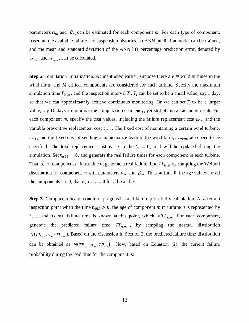
parameters 𝛼𝑚 and 𝛽𝑚 can be estimated for each component m. For each type of component,

based on the available failure and suspension histories, an ANN prediction model can be trained,

and the mean and standard deviation of the ANN life percentage prediction error, denoted by

mp , and mp , , can be calculated.

Step 2: Simulation initialization. As mentioned earlier, suppose there are N wind turbines in the

wind farm, and M critical components are considered for each turbine. Specify the maximum

simulation time 𝑇Max, and the inspection interval 𝑇𝐼. 𝑇𝐼 can be set to be a small value, say 1 day,

so that we can approximately achieve continuous monitoring. Or we can set 𝑇𝐼 to be a larger

value, say 10 days, to improve the computation efficiency, yet still obtain an accurate result. For

each component m, specify the cost values, including the failure replacement cost 𝑐𝑓,𝑚 and the

variable preventive replacement cost 𝑐𝑝,𝑚. The fixed cost of maintaining a certain wind turbine,

𝑐𝑝,𝑇, and the fixed cost of sending a maintenance team to the wind farm, 𝑐𝐹𝑎𝑟𝑚, also need to be

specified. The total replacement cost is set to be 𝐶𝑇 = 0 , and will be updated during the

simulation. Set tABS = 0, and generate the real failure times for each component in each turbine.

That is, for component m in turbine n, generate a real failure time 𝑇𝐿𝑛,𝑚 by sampling the Weibull

distribution for component m with parameters 𝛼𝑚 and 𝛽𝑚. Thus, at time 0, the age values for all

the components are 0, that is, 𝑡𝑛,𝑚 = 0 for all n and m.

Step 3: Component health condition prognostics and failure probability calculation. At a certain

inspection point when the time 𝑡𝐴𝐵𝑆 > 0, the age of component m in turbine n is represented by

𝑡𝑛,𝑚 , and its real failure time is known at this point, which is 𝑇𝐿𝑛,𝑚 . For each component,

generate the predicted failure time, 𝑇𝑃𝑛,𝑚 , by sampling the normal distribution

mnpmn TLTLN ,, , . Based on the discussion in Section 2, the predicted failure time distribution

can be obtained as mnpmn TPTPN ,, , . Now, based on Equation (2), the current failure

probability during the lead time for the component is:

13

dxeTP

dxeTP

mn

mnp

mn

mn

mn

mnp

mn

t

TP

TPx

mnp

Lt

t

TP

TPx

mnp

mn

,

2

,

,

,

,

2

,

,

2

1

,

2

1

,

,

2

1

2

1

Pr

(6)

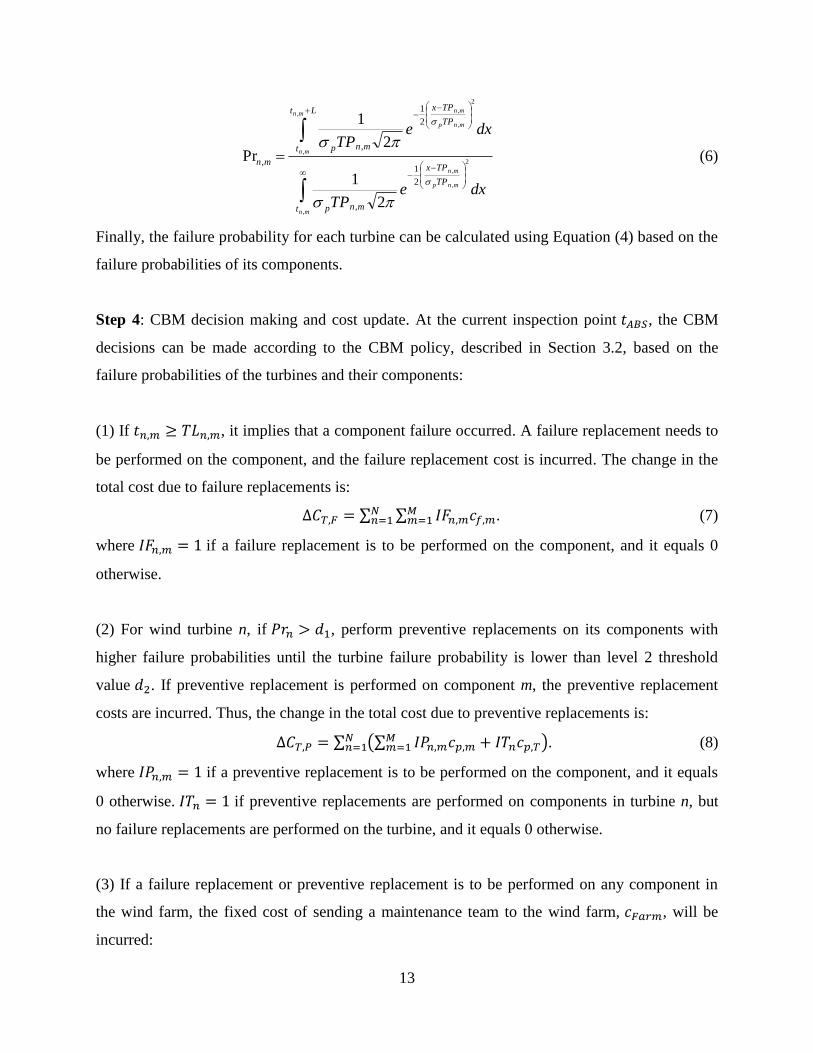
Finally, the failure probability for each turbine can be calculated using Equation (4) based on the

failure probabilities of its components.

Step 4: CBM decision making and cost update. At the current inspection point 𝑡𝐴𝐵𝑆, the CBM

decisions can be made according to the CBM policy, described in Section 3.2, based on the

failure probabilities of the turbines and their components:

(1) If 𝑡𝑛,𝑚 ≥ 𝑇𝐿𝑛,𝑚, it implies that a component failure occurred. A failure replacement needs to

be performed on the component, and the failure replacement cost is incurred. The change in the

total cost due to failure replacements is:

∆𝐶𝑇,𝐹 = ∑ ∑ 𝐼𝐹𝑛,𝑚𝑐𝑓,𝑚𝑀𝑚=1

𝑁𝑛=1 . (7)

where 𝐼𝐹𝑛,𝑚 = 1 if a failure replacement is to be performed on the component, and it equals 0

otherwise.

(2) For wind turbine n, if 𝑃𝑟𝑛 > 𝑑1, perform preventive replacements on its components with

higher failure probabilities until the turbine failure probability is lower than level 2 threshold

value 𝑑2. If preventive replacement is performed on component m, the preventive replacement

costs are incurred. Thus, the change in the total cost due to preventive replacements is:

∆𝐶𝑇,𝑃 = ∑ (∑ 𝐼𝑃𝑛,𝑚𝑐𝑝,𝑚𝑀𝑚=1 + 𝐼𝑇𝑛𝑐𝑝,𝑇)𝑁

𝑛=1 . (8)

where 𝐼𝑃𝑛,𝑚 = 1 if a preventive replacement is to be performed on the component, and it equals

0 otherwise. 𝐼𝑇𝑛 = 1 if preventive replacements are performed on components in turbine n, but

no failure replacements are performed on the turbine, and it equals 0 otherwise.

(3) If a failure replacement or preventive replacement is to be performed on any component in

the wind farm, the fixed cost of sending a maintenance team to the wind farm, 𝑐𝐹𝑎𝑟𝑚, will be

incurred:

14

∆𝐶𝑇,𝐹𝑎𝑟𝑚 = 𝐼𝐹𝑎𝑟𝑚𝑐𝐹𝑎𝑟𝑚. (9)

where 𝐼𝐹𝑎𝑟𝑚 = 1 if 𝑐𝐹𝑎𝑟𝑚 is incurred, and otherwise it equals 0. Thus, the change in the total

replacement cost at the current inspection point is:

∆𝐶𝑇 = ∆𝐶𝑇,𝐹 + ∆𝐶𝑇,𝑃 + ∆𝐶𝑇,𝐹𝑎𝑟𝑚 (10)

(4) At the current inspection point, if any replacement is to be performed, the time will be moved

to the point when the maintenance lead time has passed, i.e.,

𝑡𝐴𝐵𝑆 = 𝑡𝐴𝐵𝑆 + 𝐿. (11)

Otherwise, we will move the next inspection point:

𝑡𝐴𝐵𝑆 = 𝑡𝐴𝐵𝑆 + 𝑇𝐼. (12)

At the new inspection point, if a failure replacement or preventive replacement has been decided

to be performed on component m in turbine n, generate a new real failure time 𝑇𝐿𝑛,𝑚 by

sampling the Weibull distribution for component m with parameters 𝛼𝑚 and 𝛽𝑚. If the current

time 𝑡𝐴𝐵𝑆 has not exceeded the maximum simulation time 𝑇Max, repeat Step 3 and Step 4.

Step 5: Total replacement cost calculation. When the maximum simulation time is reached, that

is, 𝑡𝐴𝐵𝑆 = 𝑇Max, the simulation process is completed. The total replacement cost for the wind

farm can be calculated as:

𝐶𝐸 = 𝐶𝑇/𝑇Max. (13)

And the total replacement cost for each turbine is:

𝐶𝐸𝑇 =𝐶𝑇

𝑁∙𝑇Max. (14)

It should be noted that the cost measure of the maintenance policy is cost per unit of time, that is,

$/day or $/year. This cost measure corresponds to annual cost in engineering economics. If we

are interested in other discounting related measures, such as the net present value (NPV), for a

certain period of time, they can be calculated based on the annual value [24].

15

4. An example

4.1. Maintenance optimization using the proposed CBM approach

In this section, an example is used to demonstrate the proposed CBM approach for wind power

generation systems. Consider a group of 5 wind turbines, produced and maintained by a certain

manufacturer, in a wind farm at a remote site. To simplify our discussion, in this example, we

study 4 key components in each wind turbine: the rotor (including the blades), the main bearing,

the gearbox and the generator, as shown in Fig. 3 [26].

Fig. 3. Key wind turbine components considered in the example [26]

Table 1: Weibull failure time distribution parameters for major components

Component Scale parameter 𝛼

(days) Shape parameter 𝛽

Rotor 3,000 3.0

Main bearing 3,750 2.0

Gearbox 2,400 3.0

Generator 3,300 2

16

Assume the Weibull distributions are appropriate to describe the component failure times, and

the Weibull parameters are given in Table 1. The component lifetime distribution parameters are

specified based on the data given in Ref. [27] and [28]. The cost data are given in Table 2,

including the failure replacement costs for the components, the fixed and variable preventive

replacement costs and the cost of sending a maintenance team to the wind farm. The cost data are

specified based on the cost related data given in Ref. [1] and [29]. The ANN prediction method

is used to predict the failure time distributions of the wind turbine components, and suppose the

standard deviations of the ANN life percentage prediction errors are 0.12, 0.10, 0.10, and 0.12,

respectively, as shown in Table 3. The standard deviation values are selected by referring to that

estimated using the bearing degradation data in Ref [25] and [30]. The maintenance lead time is

assumed to be 30 days, and the inspection interval is set at 10 days.

Table 2: Failure replacement and preventive maintenance costs for major components

Component

Failure

replacement cost

($1000)

Variable preventive

maintenance cost

($1000)

Fixed preventive

maintenance cost

($1000)

Fixed cost to

the wind farm

($1000)

Rotor 112 28

50

Main bearing 60 15

25

Gearbox 152 38

Generator 100 25

Table 3: ANN life percentage prediction error standard deviation values for major components

Component Standard deviation

Rotor 0.12

Main bearing 0.10

Gearbox 0.12

Generator 0.10

17

The total maintenance cost can be evaluated using the proposed simulation method presented in

Section 3.3. The cost versus failure probability threshold values plot is given in Fig. 4, where the

failure probability threshold values are given in the logarithm scale. It is found that the total

maintenance cost is affected by the two failure probability threshold values, and the optimal

CBM policy exists which corresponds to the lowest cost. Optimization is performed, and the

optimal CBM policy with respect to the lowest total maintenance cost can be obtained. The

obtained optimal threshold failure probability values are: 𝑑1 = 0.1585, 𝑑2 = 3.4145 × 10−6,

and the optimal expected maintenance cost per unit of time is 577.08 $/day. Fig. 5 shows the cost

versus 𝑑1 plot while 𝑑2 is kept at 3.4145 × 10−6, and the cost versus 𝑑2 plot while 𝑑1 is kept at

0.1585 is presented in Fig. 6. These two figures can more clearly show the change in the

maintenance cost with respect to one of the failure probability threshold value around the optimal

point.

Fig. 4. Cost versus failure probability threshold values in the logarithm scale

4.2 Comparative study with the time-based maintenance policies

There are mainly two types of time-based maintenance policies: the constant-interval

maintenance policy and the age-based maintenance policy. The former is also called block

replacement policy. Under constant-interval maintenance, if a component fails, a failure

replacement will be performed right away. Preventive replacements will be performed on

-4-3

-2-1

0

-30

-20

-10

0400

600

800

1000

1200

Log(d1)Log(d

2)

Co

st (

$/d

ay)

18

Fig. 5. Cost versus threshold d1 in the logarithm scale (𝑑2 = 3.4145 × 10−6)

Fig. 6. Cost versus threshold d2 in the logarithm scale (𝑑1 = 0.1585)

components at constant intervals, say every 3 months. In age-based maintenance, a failure

replacement will also be performed right away if a component fails, and a preventive

replacement is performed once the age of the component reaches a pre-specified age value. The

age of the component is reset to 0 once a replacement is performed. For the wind power

generation systems, there are significant fixed maintenance costs on the wind farm level and on

the wind turbine level. Thus, the age-based maintenance policy is not suitable for the wind power

generation systems because these fixed maintenance costs will be incurred whenever a

preventive replacement is performed on a component when the preventive replacement age is

reached. Currently, the constant-interval maintenance policy is the maintenance policy that is

adopted the most in wind power industry [1]. So, we only investigate the constant-interval

maintenance policy in this comparative study.

-4 -3 -2 -1 0400

600

800

1000

1200

Log(d1)

Co

st (

$/d

ay)

-25 -20 -15 -10 -5 0500

600

700

800

900

Log(d2)

Co

st (

$/d

ay)

19

In the constant-interval maintenance policy, 𝑡𝐶𝐼 is used to denote the maintenance interval. The

objective of the maintenance optimization is to find the optimal 𝑡𝐶𝐼 value to minimize the

expected maintenance cost. Based on the discussion of the constant-interval maintenance policy

in Ref. [6], we can extend the method in [6] and use the following equation to calculate the total

expected maintenance cost:

CI

M

m

CIm

CI

mf

CI

mp

CIt

tHCC

NtC

1

,, )(

)( (15)

where CI

mpC , is the total cost of a failure replacement for component m, and CI

mfC , is the total cost of

a preventive replacement for component m. CIm tH denotes the expected number of failures for

component m in interval CIt,0 , which can be evaluated using a recursive procedure [6].

To ensure a fair comparison, for the constant-interval maintenance policy, we use the same

lifetime distributions for the components, as given in Table 1. We also try to use the same cost

data in Table 2. Since the fixed cost on the farm level, 𝑐𝐹𝑎𝑟𝑚, is incurred whenever a failure

replacement is performed, the failure replacement cost in Equation (15) is equal to 𝑐𝐹𝑎𝑟𝑚 plus

the failure replacement cost in Table 2, as shown in Table 4. As to the preventive replacement

cost, the turbine level fixed cost in Table 2 is shared by all the turbine components, and the wind

farm level fixed cost is shared by all the components in the wind farm. That is, the preventive

replacement cost for component m can be calculated as:

𝐶𝑓,𝑚𝐶𝐼 = 𝑐𝑝,𝑚 + 𝑐𝑝,𝑇 𝑀⁄ + 𝑐𝐹𝑎𝑟𝑚 𝑁𝑀⁄ . (16)

The calculated preventive replacement cost data using Equation (16) are also shown in Table 4.

Using Equation (15), the expected maintenance cost )( CItC can be calculated. The plot of the

cost versus the preventive maintenance interval CIt is shown in Fig. 7. As can be seen, an

optimal preventive maintenance interval with respect to the lowest cost exists. The optimal

constant-interval maintenance policy can be found using a simple optimization procedure. The

optimal preventive replacement interval is found to be 1,460 days, and the corresponding optimal

maintenance cost is 833.41 $/day. As presented in Section 4.1, using the proposed CBM

20

approach, the optimal expected maintenance cost is 577.08 $/day. Thus, a cost saving of 44.42%

can be achieved using the proposed CBM approach. The comparative study demonstrates that the

proposed CBM approach is more cost-effective comparing to the widely used constant-interval

maintenance policy.

Table 4: Cost data for the constant-interval maintenance policy

Component

Failure replacement

cost ($1000)

Preventive replacement

cost ($1000)

Rotor 162 36.75

Main bearing 110 23.75

Gearbox 202 46.75

Generator 150 33.75

Fig. 7. Cost plot for the constant-interval based preventive maintenance policy

5. Conclusions

In this paper, we proposed an optimal CBM policy to address the maintenance of wind farms

where multiple wind turbine generators are installed. The proposed maintenance policy is

0 500 1000 1500 2000 2500800

1000

1200

1400

1600

1800

2000

Preventive maintenance interval (days)

Co

st (

$/d

ay)

21

defined by two failure probability thresholds at the wind turbine level. Leveraging the condition

monitoring data, prognostics tools are devised to predict the distribution of component failure

times. Given the failure probabilities for components and the system, optimal CBM decisions

can be made on: 1) the maintenance schedule; 2) target wind turbines to be maintained; and 3)

key components to be inspected and fixed. A simulation method has been developed to evaluate

the cost of the proposed CBM policy. Numerical examples and comparative studies are presented

to illustrate and examine the effectiveness of the proposed approach. Our future efforts will

concentrate on systems where dependent failures are involved or wind farms employing

heterogeneous turbines.

Acknowledgments

This research is supported by the Natural Sciences and Engineering Research Council of Canada

(NSERC) and Le Fonds québécois de la recherche sur la nature et les technologies (FQRNT).

References

[1]. Hau E. Wind turbines: fundamentals, technologies, application, economics, Springer; 2006.

[2]. Tavner PJ, Xiang J, Spinato F. Reliability analysis for wind turbines. Wind Energy 2007;

10: 1-18.

[3]. Krokoszinski HJ. Efficiency and effectiveness of wind farms - keys to cost optimized

operation and maintenance. Renewable Energy 2003; 28(14): 2165-2178.

[4]. Sen Z. Statistical investigation of wind energy reliability and its application. Renewable

Energy 1997; 10(1): 71-79.

[5]. Martinez E, Sanz F, Pellegrini S. Life cycle assessment of a multi-megawatt wind turbine.

Renewable Energy 2009; 34(3): 667-673.

[6]. Jardine AKS, Tsang AH. Maintenance, Replacement, and Reliability Theory and

Applications, CRC Press, Taylor & Francis Group; 2006.

22

[7]. Jin T, Mechehoul M. Minimize production loss in device testing via condition based

equipment maintenance. IEEE Transactions on Automation Science & Engineering 2010;

accepted.

[8]. Liu WY, Tang BP, Jiang YH. Status and problems of wind turbine structural health

monitoring techniques in China. Renewable Energy 2010; 35(7): 1414-1418.

[9]. Hameed Z, Ahn SH, Cho YM. Practical aspects of a condition monitoring system for a

wind turbine with emphasis on its design, system architecture, testing and installation.

Renewable Energy 2010; 35(5): 879-894.

[10]. Hameed Z, Hong YS, Cho YM, Ahn SH, Song CK. Condition monitoring and fault

detection of wind turbines and related algorithms: a review. Renewable and Sustainable

Energy Reviews 2007; 13(1) 1-39.

[11]. Caselitz P, Giebhardt J. Rotor condition monitoring for improved operational safety of

offshore wind energy converters. ASME Trans. Journal of Solar Energy Engineering 2005;

127(2): 253–261.

[12]. Jeffries WQ, Chambers JA, Infield DG. Experience with bicoherence of electrical power

for condition monitoring of wind turbine blades. IEE proceedings. Vision, image and signal

processing 1998; 45(3): 141–148.

[13]. Yang W, Tavner PJ, Wilkinson MR. Condition monitoring and fault diagnosis of a wind

turbine synchronous generator drive train. Renewable Power Generation, IET 2009; 3(1) 1-

11.

[14]. Nilsson J, Bertling L. Maintenance management of wind power systems using condition

monitoring systems—life cycle cost analysis for two case studies. IEEE Transactions on

Energy Conversion 2007; 22(1) 223-229.

[15]. Byon E, Ding Y. Season-dependent condition based maintenance for a wind turbine using a

partially observed Markov decision process. IEEE Transactions on Power Systems 2010;

accepted.

[16]. Sorensen JD. Framework for Risk-based Planning of Operation and Maintenance for

Offshore Wind Turbines. Wind Energy 2009; 12: 493-506.

[17]. Marble S, Morton BP. Predicting the remaining life of propulsion system bearings. In:

Proceedings of the 2006 IEEE Aerospace Conference, Big Sky, MT, USA; 2006.

23

[18]. Kacprzynski GJ, Roemer MJ, Modgil G, Palladino A, Maynard K. Enhancement of

physics-of-failure prognostic models with system level features. In: Proceedings of the

2002 IEEE Aerospace Conference, Big Sky, MT, USA; 2002.

[19]. Li CJ, Lee H. Gear fatigue crack prognosis using embedded model, gear dynamic model

and fracture mechanics. Mechanical Systems and Signal Processing 2005; 19: 836-846.

[20]. Banjevic D, Jardine AKS, Makis V, Ennis M. A control-Limit ploicy and software for

condition based maintenance optimization. INFOR 2001; 39: 32-50.

[21]. Gebraeel N, Lawley M, Li R, Ryan JK. Life Distributions from Component Degradation

Signals: A Bayesian Approach. IIE Transactions on Quality and Reliability Engineering

2005; 37(6): 543-557.

[22]. Tian Z. An artificial neural network method for remaining useful life prediction of

equipment subject to condition monitoring. Journal of Intelligent Manufacturing 2009;

accepted. doi: 10.1007/s10845-009-0356-9.

[23]. Tian Z, Wong L, Safaei N. A neural network approach for remaining useful life prediction

utilizing both failure and suspension histories. Mechanical Systems and Signal Processing

2009; accepted. doi:10.1016/j.ymssp.2009.11.005.

[24]. Newnan DG, Whittaker J, Eschenbach TG, Lavelle JP. Engineering Economic Analysis

(Canadian Edition), Oxford University Press; 2006.

[25]. Wu B, Tian Z, Chen M. Condition based maintenance optimization using neural network

based health condition prediction. IEEE Transactions on Systems, Man, and Cybernetics--

Part A: Systems and Humans 2010; Under review.

[26]. National instruments products for wind turbine condition monitoring.

http://zone.ni.com/devzone/cda/tut/p/id/7676. 2010.

[27]. 2008-2009, “WindStats Newsletter,” 21(4)-22(3), Denmark.

[28]. Guo HT, Watson S, Tavner P. Reliability analysis for wind turbines with incomplete failure

data collected from after the date of initial installation, Reliability Engineering and System

Safety 2009; 94(6): 1057-1063.

[29]. Fingersh L, Hand M, Laxson A. Wind turbine design cost and scaling model, National

Renewable Energy Laboratory technical report; 2006.

[30]. B. Stevens, “EXAKT reduces failures at Canadian Kraft Mill,” www.modec.com; 2006.