•

•

/

Confidence Intervals on the Join Point

in Segmented Regression

By WALTER W. PIEGORSCH

Biometrics Unit, Cornell university, Ithaca, NY, USA

SUMMARY

A modified maximum likelihood estimator of the join point abscissa

in a two-phase, continuous, segmented regression model is developed.

Its sampling distribution is considered, including its moments and

variance. With the estimator, construction of confidence intervals

is undertaken, using an approximate method based on a stable variance

estimate and an exact method utilizing the join estimator's distri-

bution function. Comparisons are made to a previously derived

method based on Fieller's theorem, using a simulated and an observed

data set.

Keywords: TWO-PHASE REGRESSION; PIECEWISE REGRESSION; CONFIDENCE

t_ INTERVAL ESTIMATION; JOIN POINT

1. INTRODUCTION

IN many experimental situations, the regression relationship under consideration

is a two-phase segmented model. When the segments are constrained to intersect

at some join point, J, this model is known as a bilinear spline. The problem

of estimating J has been considered in great detail (Blischke, 1961; Hinkley,

1971), including extensions to more complicated segmentations (Hudson, 1966;

Esterby and El-Shaarawi, 1981). The results have shown that the nonlinear

nature of the problem leads to very complicated equations, some of which can

• only be solved iteratively. To ease these problems same recent works have

-2-

~ approached the problem from a decision-theoretic viewpoint (Smith and Cook,

l98o; Chin Choy and Bremeling, l98o), although the current trend has been to

~

~

suggest algorithms and alternatives which help speed the estimation process

(Ginsberg et al., l98o; Lerman, l98o; Tishler and Zang, l98la, b).

One topic of interest which has not seen much exposure is confidence

region construction; only a few papers considering it have appeared (Kasten-

baum, l959; Dathe and MUller, l98o). In general, the nonlinear nature of the

problem makes these constructions difficult, and care must be taken in develop-

ing such. We will present procedures based on a modified maximum likelihood

estimator (MLE), and consider comparisons with some previously derived procedures.

2. MODIFIED ESTJMATOR

We model the relationship from pairs of observations (x.,Y.), where xis ~ ~

an independent, fixed variable, as

(i=l,···,'t') (2.l)

(i = 't'+l, • • • ,n)

I_

(The x. 's are assumed ordered such that there is some j < -r and k> -r + l with ~

xj < x't' < x't'+l < ~ . ) The random variation in Yi is described in terms of €i'

(2.2)

For such a model, Blischke (l96l) derived the MLE by critically distinguishing

the case of 't' known. He showed that the estimator is simply the intersection

of the two sample regressions, a ratio of the form

, (2.3)

where al and 3l are the intercePt and slope MLEis, respectively, for the

•

•

•

-3-

A A

f'irst -r data pairs, and a 2 and t32 are those f'or the next n- -r data pairs. When A

J f'alls outside of' the interval Ex..-, x-r+l ], the endpoint which maximizes the

likelihood fUnction is taken as the join abscissa. [In the case -r unknown one

can either apply the procedure over all -r and choose that J(-r) which maximizes A

the likelihood as JMLE' or simply estimate -r f'irst (e.g. as in Ferreira, 1975) A

and then calculate J .] We consider, throughout, the simpler (though not

unusually restrictive) case of' -r known.

Because the MLE has no closed-f'orm expression, its sampling distribution

is dif'f'icult to derive. However, by modifying it slightly, the results become A

more tractible. Our suggestion is to simply truncate J at the endpoints of'

-the known interval and def'ine the new estimator, J, by

A

f if' J< X ... ...

"'"' A A

(2.4) J = J if' x ~J~x 1 ... '!"+ A

\..x-r+l if' J> x-r+l

Development of' the sampling behavior of' J f'ollows quickly f'rom that of' J . The

ldtter is a ratio of' correlated Normal variables, the distribution function of'

which has been developed by D.V. Hinkley (1969). In this setting it becomes

FJ(t) A (al-a2-(t32-t3l)t t31-t32 v2t-vJ?

= P[J ~ t] = L ' ; v1v2a ) v1v2a v2

(t32-t3l)t-al+a2 t32-t3l v2t-vJ? + L( ' v2 ' v1v2a ) ' v1v2a

(2.5)

where

' (2.6)

' (2.7)

•

•

•

p =

'T L = ~ X. /T ,

.L • 1 J. J.=

'T cl = ~ (x. -X.. )2 ,

. 1 J. .l J.=

-4-

n ~= ~ x./(n-T),

i='T+l J.

n c2 = ~ (x. - x2)2 ,

. 1 J. J.='!+

and L is the standard bivariate Normal integral, defined as

From (2.4) and (2.5), one can show that t_

(0 if' t< X 'T

. ,..,. l FJ(x-r) if' t=x FJ(t) = P(JS t] =~

'T

I FJ(t) if' x'T < t< x-r+l \ \1 \;:: if' t ~ x'T+l

-

(2.8)

(2.9)

(2.10)

(2.11)

The moments of' J are also as attainable. Integration by parts can be em-

ployed to show

•

•

•

-5-

x-r=l. E(J) = x-r+l. - J FJ(t)dt ' (2.1.2)

and x-r

var(J) (2.1.3) X --

't'

Again, since FJ depends upon L, values of the integrands in (2.1.2) and (2.1.3)

can be calculated, and the expressions then evaluated using a numerical quadra-

ture procedure. Simulations were carried out to examine the sampling behavior

of J, and they suggested that this modified estimator performed adequately.

Values of E(J) were commonly close to the true value of J, and the values of

var(J) were particularly smal.l. (Piegorsch, 1.982). Specific exemplifications

of the use of these equations will be presented in Section 4.

3. CONFIDENCE INTERVALS ON J

With an available, closed-form distribution fUnction in (2.1.1), we can con-

sider construction of confidence intervals on J • Mood, Graybill, and Boes

(1.974, Ch. 8) present a procedure for confidence interval construction which I_

they call 'The Statistical Method'. It involves calculating two functions of

an unknown parameter, e, from the distribution function of some estimator of

e - call it T - then solving for the confidence limits by using the observed

value of the estimator. Specifically, if the estimator produces an estimate

of t 0 then the lower limit is found by solving for e in

to

p1 = J fT(tle)dt

-=

and the upper l.imi t is found by solving for a in

p2 = J fT(tle)at

to

' (3.1.)

(3.2)

-6-

• The resulting interval will have a confidence coefficient of l- p1 - p2 (note

that pi> 0, i = 1,2, and p1 +p2 < l) •

•

•

In our setting this will be rather tricky. We do not have a simple one-

parameter distribution :function. Instead, a pair of parameters, ~l =a1 - a2

and ~2 = 132 - e1 , which contribute to the parameter of interest, J, are involved.

To get around this we will make probability statements about each parameter,

then use the Bonferroni inequality (actually just a simplified version:

P[An B] ~ P[A] + P[B]- l) to simultaneously combine the statements into one

interval (as exemplified in Lieberman et al., 1967). We will use the fact

that ~2 -N(I-12,1), then combine confidence statements based on this with state­

ments on 1-11 derived using The Statistical Method • In each case we will need

statements with probability 1- (a/2) so as to combine them into one statement

with confidence coefficient l- a . The result will be limits, ct and cu' such

that P[ c t < J < cu] ;;;:: l -a . We will need to break things up into three cases:

X < J < X l' J = X , and J = X l • T T+ T T+

(3.3)

so

(3.4)

where, for notation's sake,

and (3.5)

The Statistical Method suggests that we can solve for 1-11 in

and (3.6)

• -7-

and then take

The simultaneous combination of (3.4) and (3.7) gives us a (minimum) l-a:

interval on J, but it must be performed carefully:

(i) If ~i ~ o then [J< ~i/~2 n l/~2 < u0 ] ==> J < ~iu0 •

Now, if~~ ~o then [J>~~;~2 nl/~2 >.t0 J ==> J>1-1~.t0 • But, if

~~ < 0 then [J> ~~~~2 n l/~2< uo] ::> J> ~~uo

(ii) If ~~<0 then [J<~~/~2 nl/~2 >.t0 J ==> J<~~t0 ·

(3-7)

Also, since ~~ > ~~ by construction, ~~ < 0 so [J> ~~~~2 n l/~2 < uo]

==> J> ~~uo

-CASE II: J=x 'r

Obviously here c.~, = x-r, and we only need consider

derivation of cu' i.e., our only interest is in the value of ~i combined

• simultaneously with a bound on ~2 • The former value satisfies F;J(x-r) = l- (cx/4)

while the latter will follow from Normal distribution theory. Again, the

•

simultaneous combination can be tricky:

'- (i) ~~ ~0. Since P(~2 >G2 -v2~-l[l- (a:/2)]} = l- (a:/2), combination

with P[x-r<J<I.l.~/1.!2 ] = l-(a:/2) produces cu=~~/(~2 -v2~-l[l-(a:/2)]}. (ii) ~~ < 0 . Similar to the above, P[~2 < ~2 - v2~-1(a:/2)] = l- (a:/2),

so we get cu = 1.1i/E~2 - v2~ -l(a:/2)] . Note that ~ -l(a:/2) = -~ -l[l-(a/2)] •

"" CASE III: J=x • -r+l In this case c = x 1 and our interest is in values

u 'r+

of 1.1~ such that F:J(x-r+l) = l- (a:/4) in simultaneity with a lower or upper bonnd

on ~2 .

(i)

(ii)

The results are similar to those in Case II:

b 0 . ~l < gJ.ves

b 0 . 1.11 ~ gJ.ves

All of these results are summarized in Table l. Note that we have taken cr2 as

•

•

•

-8-

known. If this were not the case, and there were no previously establish esti-

mate to use instead, the simultaneous combination could be extended to the 3

parameters, ~l' ~2, and a2 •

-8HOW TABLE 1 :HERE-

The number of calculations involved here is formidable, and one would

probably need to turn to the computer. A question that naturally arises is

whether or not a computationally simpler procedure could be developed, at the

expense of some fixed level of confidence. Perhaps some approximate procedure,

with less computational involvement, could be formulated? We considered inter-

vals of the form (c1,c~), where

,.._ A ,_

c 1 = max[x , J- k/var(J)] t T

(3 .8)

and

c 1 = mincJ' + k/v~r(J), x 1 ] U T+ ' (3.9)

and found that var(J) was very neatly estimated by simply replacing the parame­

ters with their ML estimates in the expression for F;J(t) in (2.5). This pro-t_ A

duced an estimate, F;J, which could then replace its theoretical counterpart in

(-2.13), i.e. simply use

X X X A "' T+l J+l T+l 2

var(J) = 2xT+l I FJ(t)dt- 2 tF;r(t)dt- (I FJ(t)dt)

X T

X T

(3.10)

In considering a value for k, we found that k ~ 2 proved empirically

stable. Average interval lengths were not so large as to effectively dupli-

ca te the lmown information - i • e., an interval with c 1 = x and c 1 = x t T U T+l

imparts little additional knowledge -while the empirical confidence coeffi-

cients worked out to about 0.9 (Piegorsch, 1982). The amount of necessary,

•

•

-9-

on-line computing was also reduced. However, we reiterate the fact that these

intervals are of an ad hoc nature and can only approximately provide the ex:peri-

menter with a pre-set confidence level.

4. EXAMPLES

We exemplifY these procedures using both a simulated and an observed set

of data. Comparisons are made to a procedure suggested by M.A. Kastenbaum

(1959), which involves applying Fieller's Theorem to the ratio in (2.3). This

method re~uires solving a ~uadratic e~uation in J to calculate the lower and

upper limits. The unfortunate possibility exists, therefore, of finding two

complex roots, at which points the lower and upper limits should strictly be

set to -oo and oo, respectively. However, if such an occurrence were to happen,

in this setting, we would simply set the lower limit to x , and the upper T

limit to x-r+l • We will, for comparison's sake, use a confidence level of

y = • 90 •

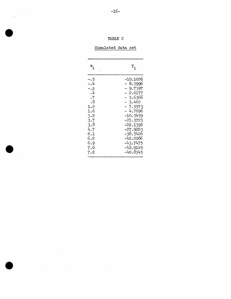
Simulated Data

1 Data were artificially produced from the model

{7. 9 + 4. 5x. + E.

~ ~

8. 9 - 7. 5x. +E. ~ ~

i = 1, ... '7

i=8,···,17 (4.1)

and E. -iid N(0,4) • The data set is presented in Table 2. Note that the true ~

join occurs at x=1.4 •

-SHOW TABLE 2 HERE-

- -To find E(J) and var(J) we need to evaluate the integrals in (2.12) and

(2.13). As mentioned earlier, the availability of specified val~es for F(t),

and therefore tF(t), makes numerical ~uadrature relatively easy. Applying the

• data values in Table 2 to (2.6), (2. 7), and (2.8) yields vf = 4.1659, 1 = 1.6542,

•

•

•

-10-

and p = 0. 3989 • Using these in (2. 5) shows

F(t) = L(4.5712t-6.3997, 9 . 3301 ; 0.4899t-0.3101) a(t) a(t)

+ L(6.3997-4.5712t, _9 _3301; o.4899t-0.310l) ,

a(t) a(t)

(4.2)

with a(t) =I (0.24-t-2 - 0. 3039t + 0.6045), f'rom (2. 9).

For a series of' values of t e [1.2,1.6], F(t), and tF(t) were calculated.

The quadrature procedure known as Simpson's Rule (Forsythe et al., 1977) was

applied over a (constant) sub-interval length of' h. = t .+1 - t. = 0.00025 • This J J J

produced approximate values with errors so small (on the order of' h4 , or about

4 X 10-15 , per sub-interval; this is a total error on the order of 10-12 ) that

the results will be considered exact. Specifically, it was fonnd that

1.6 I F(t)dt = 0.19757

1.2

and 1.6 I tF(t)dt = 0.28523

1.2

The resulting expectations were thus E(J') = 1.40243 and var(:J') = 0.02273 . As

a comparison, the asymptotic variance of theMLE (Hinkley, 1971) was calculated

f'~gm the formula

(4.3)

This produced a value of' 0.03109, almost 150% larger than var(J) •

The estimation process yielded a value of' J = 1. 2403 . Simpson's rule was

again applied to estimate the variance using (3.10), and the resulting value

A -was var(J) = 0.02lll •

The resulting 90"/o confidence intervals f'rom The Statistical Method, and

f'rom Kastenbaum's Fieller-based procedure were both f'ound to reiterate the

known information, i.e. (1.2,1.6) • The ad hoc procedure did slightly better,

•

•

-ll-

giving an interval of (l.2,l.5309) .

Liver Secretion Example

Chicken livers secrete lipids and proteins as a response to dietary flue-

tuations. For example, after imposing a change in cholesterol intake, tri-

glyceride production over time follows an increasing trend which levels off

sharply after some time period, t =J (Behr, 1982). Model (2.1) is assumed to

estimate this swi tchover time using the data in Table 3. From previous experi-

ence it is suggested that the variance about the regression model here is

well-approximated by the value cr2 = 2. 5 • The join is expected to occur between

four and six hours so that T = 3 .

-SHOW TABLE 3 HERE-

The estimation procedures in Sections 2 and 3 produce the estimates - A _,

J = 4. 7387 and var(J) = 0.1734 . Confidence intervals can be calculated using

the various methods of Section 3· They produce the following results, again at

"( = 0.9: Statistical method

Kastenbaum method

ad hoc procedure

(4.0 ,4.807 ) ,

(4.1008,5.4996) ;

(4.0 , 5. 5715)

The liver secretion results are quite pleasing, but with the simulated

data we can see that the intervals produced are not adding any sufficiently

new information to the experimental situation. One of the major reasons for

this is that the known interval lengths are small relative to the measures of -variation (e.g., vf or var(J)) involved. Since these variances are critically

dependent upon the choices of xT, xT+l' and the other design points, some ele­

ment of care must be taken when selecting the values of the x. 's • Unfortu-J.

• nately, only a few papers have appeared which consider experiment designs for

•

•

•

-12-

segmented models. Extensions of works such as Agarwal and Studden (1978), or

Park (1978) would most certainly add a great deal to the development of an

overall strategy for the statistical analysis, including interval estimation,

of segmented regressions.

5. EXTENSIONS TO UNKNOWN TAU

One critical distinction we have made is to intersect the derived confi-

dence interval with the intervlU. of known information, [x , x 1 ] . When -r 'r 'r+

is unknown, the situation becomes more complicated. Of the methods considered,·

the Kastenbaum procedure is still available, although the problem of infinite

endpoints is still of concern.

As an alternative, Hinkley (1971) has suggested approximate approaches,

based on likelihood ratios and the asymptotic Normality of MLE' s • His inter-

vals' small-sample behaviors seem empirically acceptable under the constraint

(32 = o, but when the constraint is removed, increases in variability are

observed. Further, the computations involved grow as numerous as those in

the statistical method.

What is needed is perhaps a conditional approach, first estimating -r with

some associated level of confidence, and then applying the statistical method

(or some other procedure). The opportnni ties for such improvement in join

point estimation seem endless and although burdened by very complicated models

and equations, the development of improved approaches in the estimation, test-

ing, and design of segmented models is certainly within reach.

ACKNOWLEIXIEMENTS

This research is based on the author's M.S. thesis at Cornell University,

Ithaca, NY, and was supported in part by a gran~ from Sigma Xi, The Scien-

tific Research Society. The author wishes to thank Dr. George Casella for his

many suggestions and gracious assistance, and Dr. D.S. Robson for a number of

helpful comments.

• -l3-

REFERENCES

AGARWAL, G. F. and STUDDEN, w. J. (l978). Asymptotic design and estimation

using linear splines. Commun. Statist., ~ 309-3l9.

BEHR, s. R. (l982). Personal communication.

BLISCHKE, w. R. (l96l). Least squares estimators of two intersecting lines.

Paper No. BU-l35-M in the Biometrics Unit Mimeo Series, Cornell Univers-

ity, Ithaca, NY.

CHIN CHOY, J. H. and BROEMELING, L. (l98o). Some Bayesian inferences for a

changing linear model. Technometrics, 22, 7l-78. -DATHE, E. M. and MtiLLER, P. (l980). A contribution to spline-regression.

Biometrical J., 22, 259-270. ~

ESTERBY, S. R. and EL-SHAARAWI, A. H. (l981). Inference about the point of

change in a regression model. Appl. Statist., 30, 277-285. -• FERREIRRA, P. E. (l975). A Bayesian analysis of a switching regression model:

•

Known number of regimes. J. Amer. Statist. Assoc., 70, 370-374. -FORSYTHE, G. E., MALCOIM, M. A., and MOLER, C. B. (l977). Computer Methods

for Mathematical Computations. Englewood Cliffs, NJ: Prentice-Hall.

GINSBERG, v., TISHLER, A., and ZANG, I. (l980). Alternative estimation methods

for two-regime models. Europ. Econ. Rev., 13, 207-228. ,...,... HINKLEY, D. V. (l969). On the ratio of two correlated normal random vari-

ables. Biometrika, 56, 635-639. -HINKLEY, D. V. (l97l). Inference in two-phase regression. J. Amer. Statist.

Assoc., 66, 736-743. -HUDSON, D. J. (l966). Fitting segmented curves whose join points have to be

estimated. J. Amer. Statist. Assoc., 6l, l097-ll29. -KASTENBAu.:t, M. A. (l959). A confidence interval on the point of intersection

of two fitted linear regressions. Biometrics, l5, 323-324. -

-14-

• LEIMAN, P.M. (l98o). Fitting segmented regression models by grid search.

•

•

Appl. Statist., 29, 77-84. -LIEBERMAN, G. J., MILLER, R. G., and HAMILTON, M. A. (1967). Unlimited

simultaneous discrimination intervals in regression. Biometrika, 54, ...-133-145.

MOOD, A. M., GRAYBILL, F. A., and BOES, D. C. (1974). Introduction to the

Theory o-r Statistics. New York: McGraw-Hill.

NATIONAL BUREAU OF STANDARDS (1959). Tables of the Bivariate Normal Distri-

bution Function and Related Functions. Washington, D.C.: U.S. Govern-

ment Printing Office.

PARK, S. H. (1978). Experiment designs for fitting segmented polynomial

regression models. Technometrics, 20, l5l-l54. -PIEGORSCH, w. w. (1982). A modification of the least squares join point

estimator in bilinear segmented regression. M.S. Thesis, Cornell Univers-

ity, Ithaca, NY.

SMITH, A. F. M. and COOK, D. G. (1980). Straight lines with a change point:

A Bayesian analysis of some renal transplant data. Appl. Statist., 29, -180-189.

TISHLER, A. and ZANG, I. (l98la). A maximum likelihood method for piecewise

regression models with a continuous dependent variable. Appl. Statist.,

30, 116-124. -TISHLER, A. and ZANG, I. ( l98lb). A new maximum likelihood algorithm for

piecewise regression. J. Amer. Statist. Assoc., 76, 980-987. _...

• • • TABLE 1

Statistical method confidence 1imi ts; P[ c t < J < cu J :<:: 1 -a

Case ~ satisfies ~ satisfies ll: < 0 ll: :2:: 0 IJ.~ < 0 u.f :<::0 ct c u

a - a ...... b I "' -1 a) a I "' -1 a I ~ = Fj(J) 1-~=FJ(J) X X ~ [!Ja -v2 !1? (1-~] u.1 [u.a +v2 i (1-~)]

a - a ...... b I "' -1 a ~~[~ -v:a!l?-1(1-~)] I ~ = Fj(J) 1- ~ = FJ(J) X X Ill[~ -v:a!l? (1-4)]

a ,..,. a """ b I "' -1 a a I "' -1 a I 4 = Fj(J) 1- ~= F;r(J) X X ~ [u.a +v2~ (1-4)] ~ [u.a - Va ~ (1- 4) J

II FJ(x-r) =~ a I "' -1 a - X x-r Ill [ll:a-va\1! (2)] I ...... \Jl

a I "' -1( a I

II F"'(X ) =~ X X IJ.l [!Ja-va~ 1-2)] - 1" J 1"

a ~I[~ - V:a!!? -1( 1 - ~)] III - 1- 4 - F-"(x ) X XH1 J 1"+1

a b I "' -1 a) III - 1- ~ = F"'(X ) X ~ [lla -v2\l? (2] x-r+1 J 1"+1

-l6-

• TABLE 2

Simulated data set

X. Y. l. l.

-.5 -lO.l026 -.4 - 8.5996 - ·2 - 9-73W

.4 - 2.6l77 -7 - 3.6366 .8 - 3.462

l.2 - 7. 5573 l.6 - 4.7696 3.2 -l0.5459 3·7 -2l.3723 3.8 -22.l392 4.7 -27-9223 6.l -38.5426 6.2 -42.2086 6.9 -43.7475 • 7.0 -42.9l45 7.2 -40.8345

•

-17-

• TABLE 3

Liver secretion data

Hours X. Triglyceride level yi ~

0 22.825 1 29.625 2 39.3 3 43.8 4 51.7 6 55.425 7 57-9 8 59.1 9 58.8

10 60.85 11 61.025 12 59-9625 13 6o.o625 14 58.6

• 15 61.425 16 6o.6

•