confidence is the bridge between multi-stage decisions · 2018-10-25 · article confidence is the...
TRANSCRIPT
Article
Confidence Is the Bridge between Multi-stageDecisions
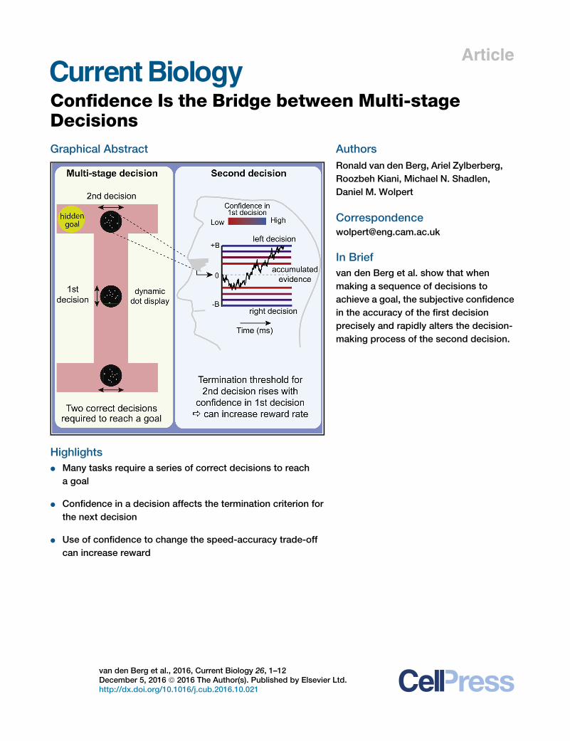
Graphical Abstract
Highlightsd Many tasks require a series of correct decisions to reach
a goal
d Confidence in a decision affects the termination criterion for
the next decision
d Use of confidence to change the speed-accuracy trade-off
can increase reward
Authors
Ronald van den Berg, Ariel Zylberberg,
Roozbeh Kiani, Michael N. Shadlen,
Daniel M. Wolpert
In Briefvan den Berg et al. show that when
making a sequence of decisions to
achieve a goal, the subjective confidence
in the accuracy of the first decision
precisely and rapidly alters the decision-
making process of the second decision.
van den Berg et al., 2016, Current Biology 26, 1–12December 5, 2016 ª 2016 The Author(s). Published by Elsevier Ltd.http://dx.doi.org/10.1016/j.cub.2016.10.021
Current Biology
Article
Confidence Is the Bridgebetween Multi-stage DecisionsRonald van den Berg,1,4 Ariel Zylberberg,2 ,4 Roozbeh Kiani,3 Michael N. Shadlen,2 and Daniel M. Wolpert1,5 ,*1Computational and Biological Learning Laboratory, Department of Engineering, Cambridge University, Cambridge CB2 1PZ, UK2Department of Neuroscience, Zuckerman Mind Brain Behavior Institute, Kavli Institute of Brain Science, and Howard Hughes MedicalInstitute, Columbia University, New York, NY 10032, USA3Center for Neural Science, New York University, New York, NY 10003, USA4Co-first author5Lead Contact*Correspondence: [email protected]://dx.doi.org/10.1016/j.cub.2016.10.021
SUMMARY
Demanding tasks often require a series of decisionsto reach a goal. Recent progress in perceptual deci-sion-making has served to unite decision accuracy,speed, and confidence in a common framework ofbounded evidence accumulation, furnishing a plat-form for the study of such multi-stage decisions. Inmany instances, the strategy applied to each deci-sion, such as the speed-accuracy trade-off, oughtto depend on the accuracy of the previous decisions.However, as the accuracy of each decision is oftenunknown to the decision maker, we hypothesizedthat subjects may carry forward a level of confidencein previous decisions to affect subsequent decisions.Subjects made two perceptual decisions sequen-tially and were rewarded only if they made bothcorrectly. The speed and accuracy of individual deci-sions were explained by noisy evidence accumula-tion to a terminating bound. We found that subjectsadjusted their speed-accuracy setting by elevatingthe termination bound on the second decision in pro-portion to their confidence in the first. The findingsreveal a novel role for confidence and a degree offlexibility, hitherto unknown, in the brain’s ability torapidly and precisely modify the mechanisms thatcontrol the termination of a decision.
INTRODUCTION
Difficult decisions arise through a process of deliberationinvolving the accumulation of evidence acquired over time.They thus invite a trade-off between speed and accuracy, instan-tiated as a rule for terminating the decision and committing to achoice [1, 2]. The speed-accuracy trade-off established throughthis rule is influenced by the cost of time weighed againstthe reward for an accurate decision and the penalty for an error[3–5]. In many instances, the regime is established throughinstruction, expertise, or some broad optimization goal, suchas maximizing reward over time. In less certain environments,
however, decision policy may benefit from adjustment on ashorter timescale [6–8]. For example, when a decision makermust complete two (or more) choices to achieve a goal, the pol-icy applied on the second choicemight be adjusted based on theprediction about the success of the first decision. These types ofmulti-stage decisions arise in foraging, exploration, and struc-tured reasoning (e.g., [9, 10]).Recent studies of single-stage perceptual decisions have
served to unite decision accuracy, speed, and confidence ina common framework of bounded evidence accumulation[11–14]. The quantitative features of this model system providea framework for studyingmulti-stage decisions. In a well-studiedmotion discrimination task, the decision itself (e.g., up or down) isgoverned by the accumulation of noisy samples of evidencefrom the visual stimulus and transduced by sensory neurons[15, 16]. The accumulation is represented by neurons in theassociation cortex such that their firing rate is proportional tothe accumulated evidence for one choice versus the other.This representation, termed a decision variable, is compared toa threshold (i.e., bound), which terminates the decision process,thereby establishing both the choice and decision time. Thelatter corresponds to the measured reaction time, but there areprocessing delays that separate these events by enough timeto allow for a dissociation between the state of accumulatedevidence used to terminate the decision and the evidenceused to support subsequent behaviors, including a change ofmind [17–19].Confidence is informed by an implicit mapping between the
state of the neural representation of accumulated evidenceused to make the decision and the likelihood that it would sup-port a correct choice [11, 20]. Since confidence can also un-dergo revision after commitment [13, 21, 22], it is possible for asubject to make a decision and believe that she made an error.Confidence thus conforms to an internal prediction about thesuccess or failure of one’s decisions. Often when a sequenceof multiple decisions are required to achieve a single goal, thesuccess of each decision is not known until the goal is reached,if ever. Therefore, as accuracy is not known, confidence is likelyto play an important role in situations that require a sequence ofdecisions to reach a goal.Here we test the hypothesis that confidence is carried forward
from a decision to control the speed-accuracy trade-off of asecond decision. Subjects made a multi-stage decision that
Current Biology 26, 1–12, December 5, 2016 ª 2016 The Author(s). Published by Elsevier Ltd. 1This is an open access article under the CC BY license (http://creativecommons.org/licenses/by/4.0/).
Please cite this article in press as: van den Berg et al., Confidence Is the Bridge between Multi-stage Decisions, Current Biology (2016), http://dx.doi.org/10.1016/j.cub.2016.10.021
involved two perceptual decisions separated briefly in time, andsuccess required both decisions to be correct. We measuredchoice and reaction time of both, and we extracted an estimateof confidence in the first decision. Subjects elevated their termi-nation criterion on the second decision in proportion to their con-fidence in the first decision. Therefore, when they were moreconfident in their first decision, they took more time and weremore accurate on their second decision, choosing a more con-servative termination criterion when building on a successfulfoundation. We show that this strategy is rational if the time tomake a decision is costly. Our results therefore point to a moregeneral capacity to adjust decision-making on a fast timescale,based on the confidence one has in a previous decision.
RESULTS
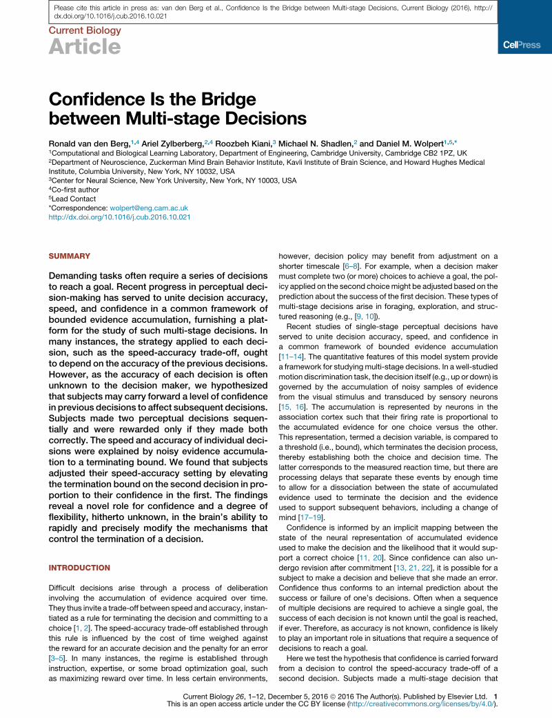
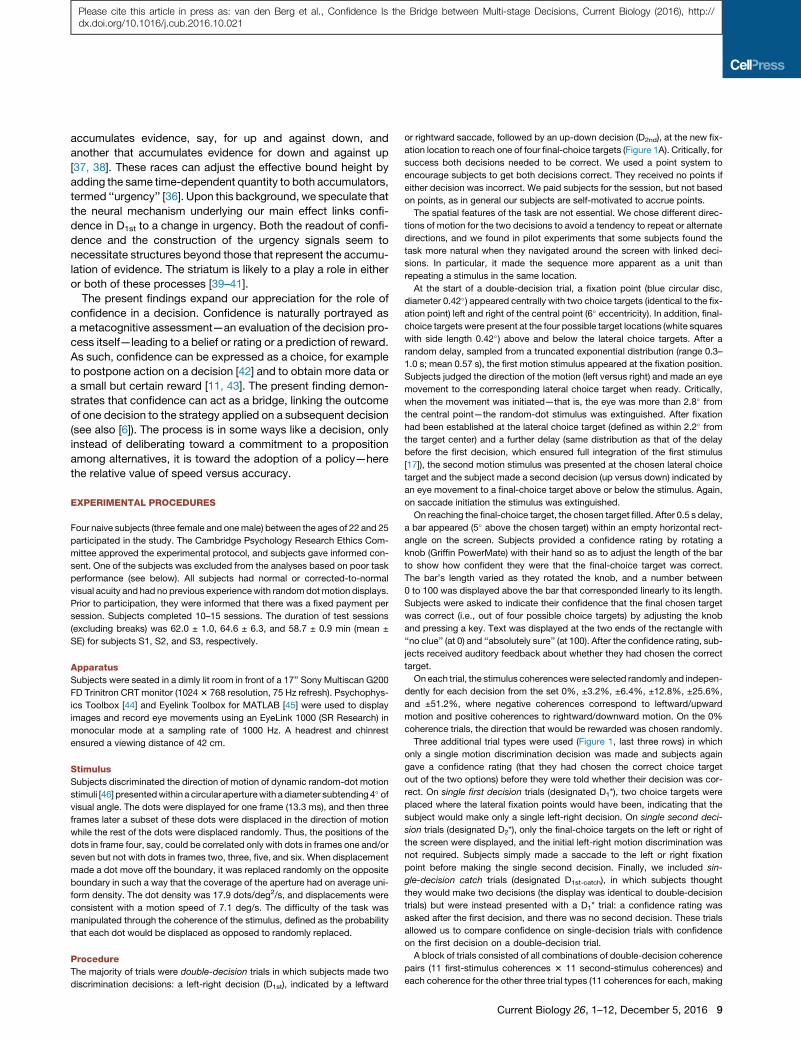
Three naive subjects were asked to decide about the net direc-tion of motion in a dynamic random-dot display (Figure 1). Boththe direction (e.g., left or right) and the strength of motion wererandom from trial to trial, and the subjects indicated their deci-sion by making an eye movement to one or the other choicetarget, whenever ready, thereby providing a measure of reactiontime. The random dot display was extinguished once the eyemovement was initiated. On most trials (Figure 1 top row), thefirst decision (D1st) led to the display of a new random dotdisplay, centered at the location of the first chosen target. Thesubject was then required to make a second decision (D2nd)about the direction of motion (up or down), again indicatedby an eye movement, when ready. The direction and motionstrength of D1st and D2nd were both random and independentlychosen. Feedback was provided only after both decisionswere made. If either choice was an error, the entire sequencewas designated as such. In other words, both decisions were
required to be correct for success on the trial (see ExperimentalProcedures). These double-decision trials (D1st then D2nd)constituted 79% of the trials. The others comprised a variety ofsingle decisions (Figure 1), most of which were explicitly cuedas such. Subjects thus knew that success on these trials restedon just one correct decision. Subjects performed a fixed numberof trials each session.All three subjects made faster and more accurate decisions
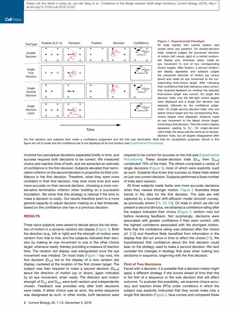
when they viewed stronger motion. Figure 2 illustrates thesetrends in the data for the first decision. The data are wellcaptured by a bounded drift-diffusion model (smooth curves),as previously shown [15, 23, 24]. On trials in which we did notpresent a second stimulus, we obtained a confidence rating afterthe subject indicated their choice (Figure 2, bottom row) butbefore receiving feedback. Not surprisingly, decisions wereassociated with greater confidence if they were correct, withthe highest confidence associated with the strongest motion.Note that the confidence rating was obtained after the choice(cf. [12]) and therefore likely benefited from information in thedisplay that did not arrive in time to affect the choice [13]. Wehypothesized that confidence about the first decision couldbear on the strategy used to make a second decision. We nextconsider the changes in strategy that arise when making twodecisions in sequence, beginning with the first decision.
First of Two DecisionsFaced with a decision, it is possible that a decision maker mightapply a different strategy if she knows ahead of time that thisis the first of a sequence or the sole decision that will affectoutcome. To evaluate this possibility, we examine choice accu-racy and reaction times (RTs) under conditions in which thesubject was explicitly instructed that they would make only asingle first decision (Figure 2, blue curves) and compared these
Fixation (0.3-1s) Decision DecisionFixation
noclue absolutely
sure
38
D1st
D1*
D2*
D2nd
Time
DoubleDecision
SingleFirst
Decision
SingleSecond
Decision
Trial Type
noclue absolutely
sure
38
noclue absolutely
sure
38
D1st-catch
SingleDecision
Catch
noclue absolutely
sure
38
Figure 1. Experimental ParadigmAll trials started with central fixation (red
circles show eye position). On double-decision
trials, subjects judged the perceived direction
of motion (left versus right) of a central random-
dot display and, whenever ready, made an
eye movement to one of two corresponding
choice targets. After fixation, a second random-
dot display appeared, and subjects judged
the perceived direction of motion (up versus
down) and made an eye movement to the cor-
responding final-choice target. After indicating
their confidence that both decisions were correct,
they received feedback on whether the selected
final-choice target was correct. On single first
decision trials, only the left-right choice targets
were displayed and a single first decision was
required, followed by the confidence judge-
ment. On single second decision trials, only one
lateral choice target and the corresponding final-
choice targets were displayed. Subjects made
an eye movement to the lateral choice target,
mimicking a first decision. Then the motion display
appeared, leading to D2*. On single-decision
catch trials, the setup was the same as on double-
decision trials, but all targets disappeared after
the first decision and subjects then made a confidence judgement and the trial was terminated. Note that for visualization purposes, stimuli in this
figure are not to scale and the confidence bar is not displayed at its true location (see Experimental Procedures).
2 Current Biology 26, 1–12, December 5, 2016
Please cite this article in press as: van den Berg et al., Confidence Is the Bridge between Multi-stage Decisions, Current Biology (2016), http://dx.doi.org/10.1016/j.cub.2016.10.021
to performance when the subject believed that the decision wasthe first of two (Figure 2, red curves). We observed only subtledifferences in decision accuracy, which were not statisticallyreliable (p > 0.36). Two subjects exhibited shorter RTs on thesingle-decision trials (reduction of S2: 90 ms; p < 0.001; reduc-tion of S3: 60 ms; p = 0.025 ANOVA). The drift-diffusion modelattributes this to a small change in k and non-decision time(Table S1). Note that this difference is not explained by a changein the termination criteria, that is, the bound height, which wouldlead to larger differences in the RTs at the lower coherences—apattern that will be apparent in the next section.From this analysis, we are unable to draw strong conclusions
about a change in decision policy induced by the need tomake two decisions in sequence. The data do not rule out thispotential strategy, but it was not exercised to great effect inthis experiment. The observation is mainly interesting whencontrasted with the subjects’ adjustments to their decisioncriteria in the second of two decisions. It will also prove conve-nient when we exploit confidence ratings from the single firstdecisions later on.
Second of Two DecisionsBoth the accuracy and RT of the second decision depended onthe experience of the first decision (Figure 3). For example, if thefirst decision resulted in an error, subjects were faster and lessaccurate on their second decision (Figure 3A, red traces) thanthey were if the first decision was correct (blue traces). Thebreakdown of the second decision by whether the first was cor-rect or an error implies that aspects of the first decision mayaffect the second decision. However, as subjects did not receivefeedback until completion of the two decisions, they could notknow if they were correct or not when they entered the seconddecision. We hypothesized that they carried forward their confi-dence after the first decision—an internal prediction or belief thatthey were correct [6, 11, 25]—to adjust criteria applied to makethe second decision.Before evaluating this hypothesis in detail, it is important to
consider plausible alternatives. Specifically, slow fluctuationsin attention or any other factors that affect the speed-accuracytrade-off on both the first and second decisions could producean association between the accuracy of the first decision and
Figure 2. Accuracy, Reaction Time, and Confidence for First DecisionsThe top andmiddle rows show the proportion of correct decisions and reaction times as a function of motion strength on single first decisions (blue: D1* trials) and
on first decisions on trials in which subjects made (or thought they would make) two decisions (red: D1st and D1st-catch trials). Solid lines are fits of a drift-diffusion
model to each dataset. The bottom row shows the confidence ratings on correct (filled) and error (open) trials for both single first decision (blue: D1*) and single-
decision catch trials (red: D1st-catch). Note that 0% trials have been designated as correct for plotting. Columns S1–S3 correspond to individual subjects. Error bars
show SEM. See also Figure S1 and Table S1.
Current Biology 26, 1–12, December 5, 2016 3
Please cite this article in press as: van den Berg et al., Confidence Is the Bridge between Multi-stage Decisions, Current Biology (2016), http://dx.doi.org/10.1016/j.cub.2016.10.021

performance on the second. We know that such fluctuationsexist in our data (Figures S1 and S2). Therefore, by selecting er-ror trials, we might have also selected trials in which the seconddecision tended to be faster and less accurate due to a commoncause (fluctuations in the decision-making process across thetwo decisions). However, co-fluctuations cannot explain threeadditional observations. First, the difficulty (motion strength) ofD1st affected both the accuracy (p < 0.01 for all subjects) andreaction times on D2nd (Figure 3B top; p < 0.0001 for all sub-jects). The difficulty is independent of any such co-fluctuationsbecause the motion strength of D1st and D2nd were uncorrelated.
Second, subjects performed single decisions similarly to thesecond of two decisions preceded by the easiest motionstrength. We examined a set of trials in which subjects madejust one decision using the identical task geometry as the secondof a sequence of decisions (labeled D2* in Figure 1). As these de-cisions are not selected based on the performance on a previous
decision, the effect of fluctuations should produce RTs repre-sented by a mixture of the D2nd RTs accompanying errors andcorrect D1st choices. The black traces in Figure 3A should there-fore lie between the redandblue traces, but thiswasnot the case.In fact, for all subjects, RTs were longest on these single deci-sions (p < 0.001 for all subjects). The force of this observationrests on the assumption that the processes underlying D2* andD2nd decisions are similar, as they appear to be. Separate fits ofthe drift-diffusionmodel to D2* and D2nd trials show no significantdifference in the signal-to-noise and non-decision time parame-ters (p > 0.3 for all subjects and parameters). In fact, the RTson D2* resemble the RTs on D2nd when the latter were precededby the strongest motion on D1st (Figure 3B bottom; p > 0.41 allsubjects). Intuitively, this is because a D2* decision, in which thesubject only needed to get this decision correct for a reward, issimilar to a D2nd decision where the subject would be certainthat the first decision was correct (e.g., highest coherence).
Figure 3. Accuracy and Reaction Time for Second Decisions(A) Data plotted against motion strength onD2nd. Trials are split bywhether the first decision was correct (blue) or an error (red). The black data points are for single
second decisions (D2*). Columns S1–S3 correspond to individual subjects, and solid lines are fits of a drift-diffusion model to each dataset.
(B) Reaction time plotted as a function of the motion strength of the first decision (D1st) for all trials (top) and split (bottom) by whether the D1st decision was correct
(blue) or an error (red). The final black data points are for trials with a single second decision (D2*).
Error bars show SEM. See also Figures S2, S3, and S5.
4 Current Biology 26, 1–12, December 5, 2016
Please cite this article in press as: van den Berg et al., Confidence Is the Bridge between Multi-stage Decisions, Current Biology (2016), http://dx.doi.org/10.1016/j.cub.2016.10.021
Third, these sequential effects were only present when the twodecisions were part of a single multi-stage decision, rather thanjust temporally adjacent. We performed the same analysis as inFigure 3B (top) but examined sequential decisions occurringacross trials (Figure S3). This showed that the RT on the firstdecision of one trial is not significantly affected by the coherenceof the decision that preceded it, that is, the last decision of theprevious trial (p > 0.19 for all subjects). This analysis providesreassurance that the effect we report depends on the groupingof the two decisions as part of the same two-stage decision pro-cess leading to a reward only if both decisions are correct. Fromtheses analyses (Figures 3B and S3), we conclude that theobserved changes in the second of two decisions are not ex-plained by factors common to both decisions or by sequentialeffects unrelated to performing the multi-stage decision task.Instead, it is an aspect of the experience of the first decisionthat affects the way the subjects approach the second. Wenext evaluate our hypothesis that the critical aspect of the firstdecision is the prediction that the first decision was correct.Figure 4 shows the confidence ratings obtained after ‘‘single
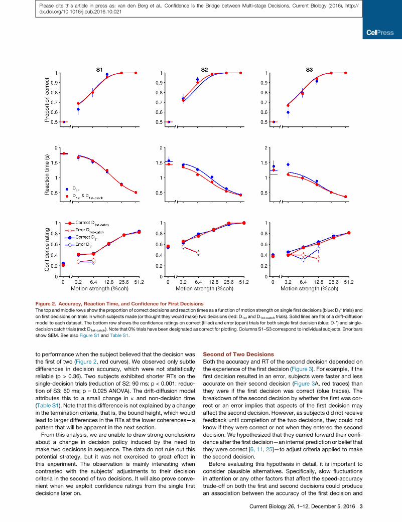
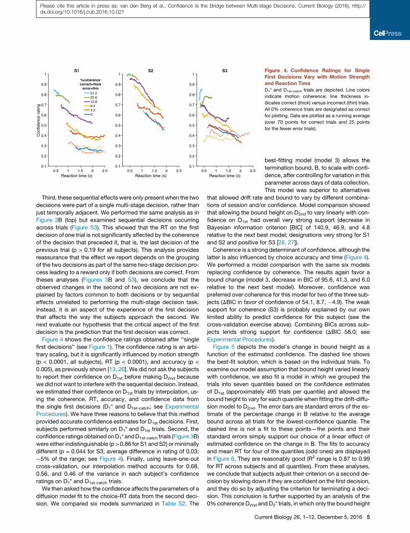
first decisions’’ (see Figure 1). The confidence rating is an arbi-trary scaling, but it is significantly influenced by motion strength(p < 0.0001, all subjects), RT (p < 0.0001), and accuracy (p <0.005), as previously shown [13, 20]. We did not ask the subjectsto report their confidence on D1st before making D2nd becausewe did not want to interfere with the sequential decision. Instead,we estimated their confidence on D1st trials by interpolation, us-ing the coherence, RT, accuracy, and confidence data fromthe single first decisions (D1* and D1st-catch; see ExperimentalProcedures). We have three reasons to believe that this methodprovided accurate confidence estimates for D1st decisions. First,subjects performed similarly on D1* and D1st trials. Second, theconfidence ratings obtained onD1* andD1st-catch trials (Figure 3B)were either indistinguishable (p > 0.86 for S1 and S2) orminimallydifferent (p = 0.044 for S3; average difference in rating of 0.03;!5% of the range; see Figure 4). Finally, using leave-one-outcross-validation, our interpolation method accounts for 0.68,0.56, and 0.46 of the variance in each subject’s confidenceratings on D1* and D1st-catch trials.We then asked how the confidence affects the parameters of a
diffusion model fit to the choice-RT data from the second deci-sion. We compared six models summarized in Table S2. The
0.5 1 1.5 2 2.5Reaction time (s)
0.1
0.2
0.3
0.4
0.5
0.6
0.7
0.8
0.9
1
Con
fiden
ce r
atin
g
S1
51.225.612.86.43.20
%coherencecorrect=thick
error=thin
0.5 1 1.5 2 2.5Reaction time (s)
0.1
0.2
0.3
0.4
0.5
0.6
0.7
0.8
0.9
1S2
0.5 1 1.5 2 2.5Reaction time (s)
0.1
0.2
0.3
0.4
0.5
0.6
0.7
0.8
0.9
1S3 Figure 4. Confidence Ratings for Single
First Decisions Vary with Motion Strengthand Reaction TimeD1* and D1st-catch trials are depicted. Line colors
indicate motion coherence; line thickness in-
dicates correct (thick) versus incorrect (thin) trials.
All 0% coherence trials are designated as correct
for plotting. Data are plotted as a running average
(over 70 points for correct trials and 25 points
for the fewer error trials).
best-fitting model (model 3) allows thetermination bound, B, to scale with confi-dence, after controlling for variation in thisparameter across days of data collection.This model was superior to alternatives
that allowed drift rate and bound to vary by different combina-tions of session and/or confidence. Model comparison showedthat allowing the bound height on D2nd to vary linearly with con-fidence on D1st had overall very strong support (decrease inBayesian information criterion [BIC] of 140.9, 46.9, and 4.8relative to the next best model; designations very strong for S1and S2 and positive for S3 [26, 27]).Coherence is a strong determinant of confidence, although the
latter is also influenced by choice accuracy and time (Figure 4).We performed a model comparison with the same six modelsreplacing confidence by coherence. The results again favor abound change (model 3, decrease in BIC of 95.6, 41.3, and 6.0relative to the next best model). Moreover, confidence waspreferred over coherence for this model for two of the three sub-jects (DBIC in favor of confidence of 54.1, 8.7, "4.9). The weaksupport for coherence (S3) is probably explained by our ownlimited ability to predict confidence for this subject (see thecross-validation exercise above). Combining BICs across sub-jects lends strong support for confidence (DBIC 58.0; seeExperimental Procedures).Figure 5 depicts the model’s change in bound height as a
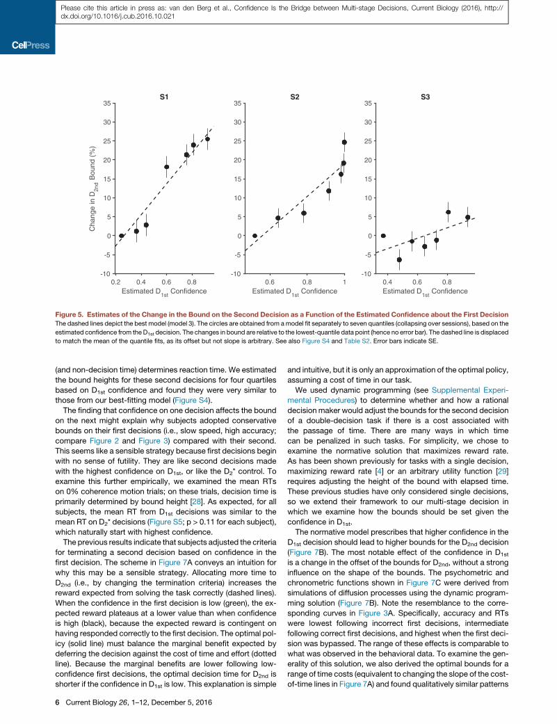
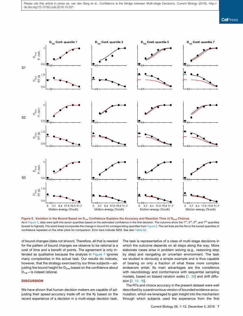
function of the estimated confidence. The dashed line showsthe best-fit solution, which is based on the individual trials. Toexamine our model assumption that bound height varied linearlywith confidence, we also fit a model in which we grouped thetrials into seven quantiles based on the confidence estimatesof D1st (approximately 495 trials per quantile) and allowed thebound height to vary for each quantile when fitting the drift-diffu-sion model to D2nd. The error bars are standard errors of the es-timate of the percentage change in B relative to the averagebound across all trials for the lowest-confidence quantile. Thedashed line is not a fit to these points—the points and theirstandard errors simply support our choice of a linear effect ofestimated confidence on the change in B. The fits to accuracyand mean RT for four of the quantiles (odd ones) are displayedin Figure 6. They are reasonably good (R2 range is 0.87 to 0.99for RT across subjects and all quantiles). From these analyses,we conclude that subjects adjust their criterion on a second de-cision by slowing down if they are confident on the first decision,and they do so by adjusting the criterion for terminating a deci-sion. This conclusion is further supported by an analysis of the0%coherence D2nd and D2* trials, in which only the bound height
Current Biology 26, 1–12, December 5, 2016 5
Please cite this article in press as: van den Berg et al., Confidence Is the Bridge between Multi-stage Decisions, Current Biology (2016), http://dx.doi.org/10.1016/j.cub.2016.10.021
(and non-decision time) determines reaction time. We estimatedthe bound heights for these second decisions for four quartilesbased on D1st confidence and found they were very similar tothose from our best-fitting model (Figure S4).
The finding that confidence on one decision affects the boundon the next might explain why subjects adopted conservativebounds on their first decisions (i.e., slow speed, high accuracy;compare Figure 2 and Figure 3) compared with their second.This seems like a sensible strategy because first decisions beginwith no sense of futility. They are like second decisions madewith the highest confidence on D1st, or like the D2* control. Toexamine this further empirically, we examined the mean RTson 0% coherence motion trials; on these trials, decision time isprimarily determined by bound height [28]. As expected, for allsubjects, the mean RT from D1st decisions was similar to themean RT on D2* decisions (Figure S5; p > 0.11 for each subject),which naturally start with highest confidence.
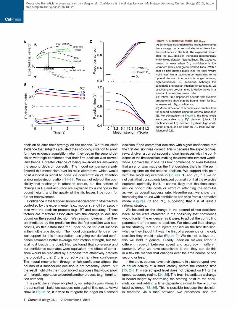
The previous results indicate that subjects adjusted the criteriafor terminating a second decision based on confidence in thefirst decision. The scheme in Figure 7A conveys an intuition forwhy this may be a sensible strategy. Allocating more time toD2nd (i.e., by changing the termination criteria) increases thereward expected from solving the task correctly (dashed lines).When the confidence in the first decision is low (green), the ex-pected reward plateaus at a lower value than when confidenceis high (black), because the expected reward is contingent onhaving responded correctly to the first decision. The optimal pol-icy (solid line) must balance the marginal benefit expected bydeferring the decision against the cost of time and effort (dottedline). Because the marginal benefits are lower following low-confidence first decisions, the optimal decision time for D2nd isshorter if the confidence in D1st is low. This explanation is simple
and intuitive, but it is only an approximation of the optimal policy,assuming a cost of time in our task.We used dynamic programming (see Supplemental Experi-
mental Procedures) to determine whether and how a rationaldecision maker would adjust the bounds for the second decisionof a double-decision task if there is a cost associated withthe passage of time. There are many ways in which timecan be penalized in such tasks. For simplicity, we chose toexamine the normative solution that maximizes reward rate.As has been shown previously for tasks with a single decision,maximizing reward rate [4] or an arbitrary utility function [29]requires adjusting the height of the bound with elapsed time.These previous studies have only considered single decisions,so we extend their framework to our multi-stage decision inwhich we examine how the bounds should be set given theconfidence in D1st.The normative model prescribes that higher confidence in the
D1st decision should lead to higher bounds for the D2nd decision(Figure 7B). The most notable effect of the confidence in D1st
is a change in the offset of the bounds for D2nd, without a stronginfluence on the shape of the bounds. The psychometric andchronometric functions shown in Figure 7C were derived fromsimulations of diffusion processes using the dynamic program-ming solution (Figure 7B). Note the resemblance to the corre-sponding curves in Figure 3A. Specifically, accuracy and RTswere lowest following incorrect first decisions, intermediatefollowing correct first decisions, and highest when the first deci-sion was bypassed. The range of these effects is comparable towhat was observed in the behavioral data. To examine the gen-erality of this solution, we also derived the optimal bounds for arange of time costs (equivalent to changing the slope of the cost-of-time lines in Figure 7A) and found qualitatively similar patterns
0.2 0.4 0.6 0.8Estimated D
1st Confidence
-10
-5
0
5
10
15
20
25
30
35
Cha
nge
in D
2nd B
ound
(%
)S1
0.6 0.8 1Estimated D
1st Confidence
-10
-5
0
5
10
15
20
25
30
35S2
0.4 0.6 0.8Estimated D
1st Confidence
-10
-5
0
5
10
15
20
25
30
35S3
Figure 5. Estimates of the Change in the Bound on the Second Decision as a Function of the Estimated Confidence about the First DecisionThe dashed lines depict the best model (model 3). The circles are obtained from amodel fit separately to seven quantiles (collapsing over sessions), based on the
estimated confidence from the D1st decision. The changes in bound are relative to the lowest-quantile data point (hence no error bar). The dashed line is displaced
to match the mean of the quantile fits, as its offset but not slope is arbitrary. See also Figure S4 and Table S2. Error bars indicate SE.
6 Current Biology 26, 1–12, December 5, 2016
Please cite this article in press as: van den Berg et al., Confidence Is the Bridge between Multi-stage Decisions, Current Biology (2016), http://dx.doi.org/10.1016/j.cub.2016.10.021
of bound changes (data not shown). Therefore, all that is neededfor the pattern of bound changes we observe to be rational is acost of time and a benefit of points. The agreement is only in-tended as qualitative because the analysis in Figure 7 ignoresmany complexities in the actual task. Our results do indicate,however, that the strategy exercised by our three subjects—ad-justing the bound height for D2nd based on the confidence aboutD1st—is indeed rational.
DISCUSSION
We have shown that human decision makers are capable of ad-justing their speed-accuracy trade-off on the fly based on therecent experience of a decision in a multi-stage decision task.
The task is representative of a class of multi-stage decisions inwhich the outcome depends on all steps along the way. Moreelaborate cases arise in problem solving (e.g., reasoning stepby step) and navigating an uncertain environment. The taskwe studied is obviously a simple example and is thus capableof bearing on only a fraction of what these more complexendeavors entail. Its main advantages are the consiliencewith neurobiology and conformance with sequential samplingmodels, based on biased random walks [1, 30] and drift diffu-sion [2, 15, 16].The RTs and choice accuracy in the present dataset were well
described by a parsimonious version of bounded evidence accu-mulation, which we leveraged to gain insight into the mechanismthrough which subjects used the experience from the first
Figure 6. Variation in the Bound Based on D1st Confidence Explains the Accuracy and Reaction Time of D2nd ChoicesAs in Figure 5, data were split into seven quantiles based on the estimated confidence in the first decision. The columns show the 1st, 3rd, 5th, and 7th quantiles
(lowest to highest). Fits (solid lines) incorporate the change in bound for corresponding quantiles from Figure 5. The red lines are the fits to the lowest quantiles of
confidence repeated on the other plots for comparison. Error bars indicate SEM. See also Table S2.
Current Biology 26, 1–12, December 5, 2016 7
Please cite this article in press as: van den Berg et al., Confidence Is the Bridge between Multi-stage Decisions, Current Biology (2016), http://dx.doi.org/10.1016/j.cub.2016.10.021
decision to alter their strategy on the second. We found clearevidence that subjects adjusted their stopping criterion to allowfor more evidence acquisition when they began the second de-cision with high confidence that their first decision was correct(and hence a greater chance of being rewarded for answeringthe second decision correctly). The model comparison clearlyfavored this mechanism over its main alternative, which wouldposit a boost in signal to noise via concentration of attentionand/or noise decorrelation [31–33]. We cannot rule out the pos-sibility that a change in attention occurs, but the pattern ofchanges in RT and accuracy are explained by a change in thebound height, and the quality of the fits leaves little room forfurther improvement.
Confidence in the first decision is associatedwith other factorscontrolled by the experimenter (e.g., motion strength) or associ-ated with the decision process (e.g., RT and accuracy). Thesefactors are therefore associated with the change in decisionbound on the second decision. We reason, however, that theyare mediated by the prediction that the first decision was suc-cessful, as this establishes the upper bound for joint successin the multi-stage decision. The model comparison lends empir-ical support for this interpretation, assigning our derived confi-dence estimates better leverage than motion strength, but thatis almost beside the point. Had we found that coherence andour confidence estimates were equivalent, the effect of coher-ence would be mediated by a process that effectively predictsthe probability that D1st is correct—that is, infers confidence.The neural mechanism through which confidence affects thebounds of a subsequent decision is not presently known, butthe result highlights the importance of a process that would allowan inferential operation to control another process (e.g., termina-tion criterion).
The particular strategy adopted by our subjects was rational inthe sense that it balances success rate against time costs. As weshow in Figure 7A, it is wise to integrate for longer on a second
decision if one enters that decision with higher confidence thatthe first decision was correct. This is because the expected finalreward, given a correct second choice, increases with the confi-dence of the first decision, making the extra time invested worth-while. Conversely, if one has low confidence or even believesthat an error was made on the first decision, there is little pointspending time on the second decision. We support this pointwith the modeling exercise in Figures 7B and 7C, but we donot claim that our subjects behaved optimally or that the exercisecaptures optimality itself. It seems likely that the time costsinclude opportunity costs or effort of attending the stimulusas well as overall success rate. Nevertheless, we show thatincreasing the boundwith confidence can arise from a normativemodel (Figures 7B and 7C), suggesting that it is at least arational strategy.We focused on the change in the second of two decisions
because we were interested in the possibility that confidencewould furnish the evidence, as it were, to adjust the controllingparameters of the second decision. We observed little changein the strategy that our subjects applied on the first decision,whether they thought it was the first of a sequence or the onlydecision they would make (Figure 2). We do not believe thatthis will hold in general. Clearly, decision makers adopt adifferent trade-off between speed and accuracy in differentcontexts. What we have established is that they can do thisin a flexible manner that changes over the time course of onesecond or less.In the brain, bounds have their signature in a stereotyped level
of neural activity at a short latency before the reaction time[15, 24]. This stereotyped level does not depend on RT or thespeed-accuracy regime [34, 35]. The brain instantiates a changein bound height by controlling the starting point of the accu-mulation and adding a time-dependent signal to the accumu-lated evidence [35, 36]. This is possible because the decisionis rendered via a race between two processes, one that
Pro
port
ion
corr
ect
0.4
0.6
0.8
1
Time (s)0 1 2 3
Dec
isio
n va
riabl
e
-1
-0.5
0
0.5
1
Motion strength (%coh)0 3.2 6.4 12.8 25.6 51.2
Rea
ctio
n tim
e (s
)
0.4
0.6
0.8
1
1.2
C
Errors D1st
Correct D1st
D2*
B
A
Exp
ecte
d tr
ial r
ewar
d
optimum
High conf. D1st
Low conf. D1st
1.00.80.6
0
cost-freeworld
totalreward
cost of time
D2nd decision time
D1stconf.
Figure 7. Normative Model for D2nd
(A) Schematic illustration of the impetus to change
the strategy on a second decision, based on
the confidence in the first. The expected reward
after the D1st decision increases monotonically
with viewing duration (dashed lines). The expected
reward is lower when D1st confidence is low
(compare black and green dashed lines). With a
cost on time (dotted black line), the total reward
(solid lines) has a maximum corresponding to the
optimal decision time, which is longer following
high-confidence D1st decisions. Although this
schematic provides an intuition for our results, we
used dynamic programming to derive the optimal
solution to maximize reward rate.
(B) Optimal time-dependent bounds from dynamic
programming show that the bound height for D2nd
increases with D1st confidence.
(C) Model simulation of accuracy and reaction time
for second decisions using the optimal bounds in
(B). For comparison to Figure 3, the three levels
are comparable to a D2* decision (black: full
confidence of 1.0), correct D1st (blue: high confi-
dence of 0.8), and an error on D1st (red: low con-
fidence of 0.6).
8 Current Biology 26, 1–12, December 5, 2016
Please cite this article in press as: van den Berg et al., Confidence Is the Bridge between Multi-stage Decisions, Current Biology (2016), http://dx.doi.org/10.1016/j.cub.2016.10.021
accumulates evidence, say, for up and against down, andanother that accumulates evidence for down and against up[37, 38]. These races can adjust the effective bound height byadding the same time-dependent quantity to both accumulators,termed ‘‘urgency’’ [36]. Upon this background, we speculate thatthe neural mechanism underlying our main effect links confi-dence in D1st to a change in urgency. Both the readout of confi-dence and the construction of the urgency signals seem tonecessitate structures beyond those that represent the accumu-lation of evidence. The striatum is likely to a play a role in eitheror both of these processes [39–41].The present findings expand our appreciation for the role of
confidence in a decision. Confidence is naturally portrayed asa metacognitive assessment—an evaluation of the decision pro-cess itself—leading to a belief or rating or a prediction of reward.As such, confidence can be expressed as a choice, for exampleto postpone action on a decision [42] and to obtain more data ora small but certain reward [11, 43]. The present finding demon-strates that confidence can act as a bridge, linking the outcomeof one decision to the strategy applied on a subsequent decision(see also [6]). The process is in some ways like a decision, onlyinstead of deliberating toward a commitment to a propositionamong alternatives, it is toward the adoption of a policy—herethe relative value of speed versus accuracy.
EXPERIMENTAL PROCEDURES
Four naive subjects (three female and onemale) between the ages of 22 and 25
participated in the study. The Cambridge Psychology Research Ethics Com-
mittee approved the experimental protocol, and subjects gave informed con-
sent. One of the subjects was excluded from the analyses based on poor task
performance (see below). All subjects had normal or corrected-to-normal
visual acuity and had no previous experiencewith randomdotmotion displays.
Prior to participation, they were informed that there was a fixed payment per
session. Subjects completed 10–15 sessions. The duration of test sessions
(excluding breaks) was 62.0 ± 1.0, 64.6 ± 6.3, and 58.7 ± 0.9 min (mean ±
SE) for subjects S1, S2, and S3, respectively.
ApparatusSubjects were seated in a dimly lit room in front of a 17’’ Sony Multiscan G200
FD Trinitron CRT monitor (10243 768 resolution, 75 Hz refresh). Psychophys-
ics Toolbox [44] and Eyelink Toolbox for MATLAB [45] were used to display
images and record eye movements using an EyeLink 1000 (SR Research) in
monocular mode at a sampling rate of 1000 Hz. A headrest and chinrest
ensured a viewing distance of 42 cm.
StimulusSubjects discriminated the direction of motion of dynamic random-dot motion
stimuli [46] presentedwithin a circular aperturewith adiameter subtending4# of
visual angle. The dots were displayed for one frame (13.3 ms), and then three
frames later a subset of these dots were displaced in the direction of motion
while the rest of the dots were displaced randomly. Thus, the positions of the
dots in frame four, say, could be correlated only with dots in frames one and/or
seven but not with dots in frames two, three, five, and six. When displacement
made a dot move off the boundary, it was replaced randomly on the opposite
boundary in such a way that the coverage of the aperture had on average uni-
form density. The dot density was 17.9 dots/deg2/s, and displacements were
consistent with a motion speed of 7.1 deg/s. The difficulty of the task was
manipulated through the coherence of the stimulus, defined as the probability
that each dot would be displaced as opposed to randomly replaced.
ProcedureThe majority of trials were double-decision trials in which subjects made two
discrimination decisions: a left-right decision (D1st), indicated by a leftward
or rightward saccade, followed by an up-down decision (D2nd), at the new fix-
ation location to reach one of four final-choice targets (Figure 1A). Critically, for
success both decisions needed to be correct. We used a point system to
encourage subjects to get both decisions correct. They received no points if
either decision was incorrect. We paid subjects for the session, but not based
on points, as in general our subjects are self-motivated to accrue points.
The spatial features of the task are not essential. We chose different direc-
tions of motion for the two decisions to avoid a tendency to repeat or alternate
directions, and we found in pilot experiments that some subjects found the
task more natural when they navigated around the screen with linked deci-
sions. In particular, it made the sequence more apparent as a unit than
repeating a stimulus in the same location.
At the start of a double-decision trial, a fixation point (blue circular disc,
diameter 0.42#) appeared centrally with two choice targets (identical to the fix-
ation point) left and right of the central point (6# eccentricity). In addition, final-
choice targets were present at the four possible target locations (white squares
with side length 0.42#) above and below the lateral choice targets. After a
random delay, sampled from a truncated exponential distribution (range 0.3–
1.0 s; mean 0.57 s), the first motion stimulus appeared at the fixation position.
Subjects judged the direction of the motion (left versus right) and made an eye
movement to the corresponding lateral choice target when ready. Critically,
when the movement was initiated—that is, the eye was more than 2.8# from
the central point—the random-dot stimulus was extinguished. After fixation
had been established at the lateral choice target (defined as within 2.2# from
the target center) and a further delay (same distribution as that of the delay
before the first decision, which ensured full integration of the first stimulus
[17]), the second motion stimulus was presented at the chosen lateral choice
target and the subject made a second decision (up versus down) indicated by
an eye movement to a final-choice target above or below the stimulus. Again,
on saccade initiation the stimulus was extinguished.
On reaching the final-choice target, the chosen target filled. After 0.5 s delay,
a bar appeared (5# above the chosen target) within an empty horizontal rect-
angle on the screen. Subjects provided a confidence rating by rotating a
knob (Griffin PowerMate) with their hand so as to adjust the length of the bar
to show how confident they were that the final-choice target was correct.
The bar’s length varied as they rotated the knob, and a number between
0 to 100 was displayed above the bar that corresponded linearly to its length.
Subjects were asked to indicate their confidence that the final chosen target
was correct (i.e., out of four possible choice targets) by adjusting the knob
and pressing a key. Text was displayed at the two ends of the rectangle with
‘‘no clue’’ (at 0) and ‘‘absolutely sure’’ (at 100). After the confidence rating, sub-
jects received auditory feedback about whether they had chosen the correct
target.
On each trial, the stimulus coherenceswere selected randomly and indepen-
dently for each decision from the set 0%, ±3.2%, ±6.4%, ±12.8%, ±25.6%,
and ±51.2%, where negative coherences correspond to leftward/upward
motion and positive coherences to rightward/downward motion. On the 0%
coherence trials, the direction that would be rewarded was chosen randomly.
Three additional trial types were used (Figure 1, last three rows) in which
only a single motion discrimination decision was made and subjects again
gave a confidence rating (that they had chosen the correct choice target
out of the two options) before they were told whether their decision was cor-
rect. On single first decision trials (designated D1*), two choice targets were
placed where the lateral fixation points would have been, indicating that the
subject would make only a single left-right decision. On single second deci-
sion trials (designated D2*), only the final-choice targets on the left or right of
the screen were displayed, and the initial left-right motion discrimination was
not required. Subjects simply made a saccade to the left or right fixation
point before making the single second decision. Finally, we included sin-
gle-decision catch trials (designated D1st-catch), in which subjects thought
they would make two decisions (the display was identical to double-decision
trials) but were instead presented with a D1* trial: a confidence rating was
asked after the first decision, and there was no second decision. These trials
allowed us to compare confidence on single-decision trials with confidence
on the first decision on a double-decision trial.
A block of trials consisted of all combinations of double-decision coherence
pairs (11 first-stimulus coherences 3 11 second-stimulus coherences) and
each coherence for the other three trial types (11 coherences for each, making
Current Biology 26, 1–12, December 5, 2016 9
Please cite this article in press as: van den Berg et al., Confidence Is the Bridge between Multi-stage Decisions, Current Biology (2016), http://dx.doi.org/10.1016/j.cub.2016.10.021
33 trials), making 154 trials in total. Subjects completed nine sessions (on
separate days) and performed four blocks in each session. Stimuli in the first
block of a session were all unique. Stimuli in the second block were mirrored
versions (horizontally or vertically as appropriate) of the stimuli in the first
block. The third and fourth blocks were identical to the first two blocks. The
order in which trials were presented was randomized in all blocks. To motivate
subjects after each block, their percentage performance over the last block
was displayed.
All subjects received extensive training over a number of days on the motion
task, in three phases: (1) D1* trials with computer-controlled variable-duration
viewing and no confidence ratings (864 trials completed in a single session), (2)
D1* and D2* trials without confidence ratings (864 trials per session until choice
and reaction times appeared stable; three sessions for subjects S1 and S2,
and five sessions for S3), and (3) double-decision trials (99 trials without
confidence ratings followed by 154 with confidence ratings). All training was
completed before the nine experimental sessions were run.
We required subjects to have sufficient perceptual skills and motivation
to perform the task. One subject became unmotivated as the sessions pro-
ceeded (failing to turn up for sessions), and an analysis of his first three ses-
sions showed that he also had very strong response bias (e.g., 90% upward
responses at 0% coherence trials), so he did not continue in the experiment
and we excluded his data from analysis.
AnalysisFor each trial, we recorded the choice and reaction time (RT; time tomovement
initiation from start of motion stimulus) for each decision as well as the final
confidence rating (which we divided by 100 so as to be on a 0–1 scale).
We refer to the two decisions of the double decision as D1st and D2nd to
distinguish them from single first and single second decisions (D1* and D2*,
respectively) and the decision made on a single-decision catch trial D1st-catch.
To examine whether accuracy on D2nd is affected by the coherence on D1st,
we performed logistic regression on D2nd choices as a function of coherence
on D2nd,
PrightðD2ndÞ= ½1+ expð " ðk1 + k2 coh2 + k3 coh2jcoh1 j ÞÞ'"1;
with the null hypothesis that k3 = 0.
To examine whether accuracy on D2nd is affected by accuracy on D1st, we
used a chi-square test with Yates correction. To compare reaction times be-
tween conditions, we performed ANOVAs on individual subjects with reaction
time (individual trials) as a function of condition and absolute coherence (as a
categorical variable).
To examine whether the confidence rating on a first decision depended
on whether subjects expected to make second decision, we performed
ANOVAs of confidence rating with factors of trial type (D1* versus D1st-catch),
motion strength (six levels), and accuracy of D1st (correct versus error). To
examine whether the individual confidence rating on a first decision depended
on the trial’s coherence, RT, and accuracy, we performed an ANOVA on the
confidence ratings with categorical factors of unsigned coherence and accu-
racy, and linear factor RT.
By design, our task does not introduce an interruption between the first and
second decision (D1st and D2nd). Thus, we did not solicit confidence reports for
D1st and instead estimated these ratings using the D1* and D1st-catch trials. For
each D1st decision, we selected a fixed number (k) of D1* and D1st-catch trials for
the same coherence and accuracy (error versus correct) that were closest to
the D1st RT and averaged the corresponding confidence ratings (k-nearest
neighbor interpolation). We chose k = 30 for correct trials and k = 15 for error
trials because errors were less frequent than correct responses. This allowed
us to generate estimates of confidence for all D1st trials to examine how the
confidence affected D2nd on the same trial.
Naturally, confidence can vary even for trials with the same motion strength,
choice, and reaction time. We therefore examined the predictive power of our
approach with leave-one-out cross-validation on D1* and D1st-catch trials. For
each D1* and D1st-catch trial, we used the data with the same coherence and
accuracy (error versus correct) to predict the confidence on that trial (leaving
that trial out of the dataset for the k-nearest neighbor). We repeated this for
all of the trials so that we have a leave-one-out prediction of confidence for
each trial as well as the actual confidence rating on that trial. We report the
fraction of variance explained from these trials.
ModelWe used a variant of the drift-diffusion model [23, 47] to explain the proportion
of choices and reaction times. The model posits that evidence accumulates
from zero until it reaches an upper or lower bound (±B), which determines
the initial choice and decision time. The increments of evidence are idealized
as normally distributed random variables with unit variance per second and
mean k(C+C0), where C is signed motion strength (specified as the proportion
of dots moving in net motion direction, positive = rightward/downward and
negative = leftward/upward motion); k, B and C0 are free parameters. The
parameters B and k explain the trade-off between speed and accuracy of
the initial choices; C0 is a coherence offset, which explains bias (if any) for
one of the choices (starting point bias versus drift bias; see Supplemental
Experimental Procedures). The RT incorporates additional latencies, termed
the non-decision time (tnd), from stimulus onset to the beginning of the
bounded accumulation process and from the termination of the process to
the beginning of the motor response.
To fit the accuracy and reaction time of the D2nd and D2* choices, we mini-
mized the negative log likelihood, using Bernoulli distributions for the choices
and Gaussian distributions for the RTs. For analytic simplicity (see below), we
used a flat bound (i.e., stationary rather than collapsing), which does not cap-
ture the shape of the RT distributions and themean RT on error trials [4]. There-
fore, for the RT component of the response likelihood for each trial, we used
only the model’s predicted mean RT and used the associated standard devi-
ation from the data for correct trials for the same coherence. Absent bias, cor-
rect choices would be rightward choices for positive coherences, leftward
choices for negative coherences, and all choices for 0%coherence. In general,
these are the direction of the more numerous choices at each coherence,
including 0. In practice, we identified the correct trials, when fitting RT, by
finding the point of subjective equality in a simple logistic fit to choice and se-
lecting rightward choice trials when pright > 0.5 and leftward choice trials for
pright < 0.5. We did not use the logistic fit to estimate C0. We optimized using
the MATLAB function fmincon using analytic gradients.
We used this parsimonious version of the bounded evidence accumulation
model, which employs stationary (i.e., flat) bounds. We recognize that the
normative prescription for terminating bounds in our experiment incorporates
non-stationary (collapsing) bounds [4]. We did not incorporate this degree of
complexity in our main model fits in order to reduce complexity and to focus
on a single bound parameter (i.e., bound height). This strategy also allowed
derivation of model gradients and Hessians allowing efficient and reliable
fitting of our models. This practice provides stable estimates of the key param-
eters (B, k, tnd).
We examined the stability of the model parameters over the nine sessions
and discovered significant variation in the bound parameter (B) and more sub-
tle variation in the other parameters. Furthermore, the values of B covaried for
D1st and D2nd (Figure S1). The likelihoods associated with reaction times were
calculated using the sample standard deviation separately for each session,
subject, and coherence.
To examine how confidence in D1st affected the parameters of the drift-
diffusion process accounting for D2nd and D2* (for which confidence was
set to 1), we compared six models (Table S2). We allowed some parameters
(B and k) to vary for each session, whereas other parameters such as C0
and tnd were shared across all sessions. Table S2 lists the parameters
that vary. Here we provide a more intuitive guide. Across the six models,
the bound (B) and the signal-to-noise term (k) can vary, and they can
do so in three ways: fixed, by session, and linearly as a function of D1st con-
fidence. Models 1 and 2 are the simplest: either B or k varies with session,
but neither depends on D1st confidence. Models 3 and 4 parallel models 1
and 2, but with an additional variation of B or k linearly with D1st confidence.
Finally, models 5 and 6 allow variation in one parameter, by session, and in
the other parameter linearly with D1st confidence. We used the Bayesian in-
formation criterion (BIC) to compare the models by controlling for their
differing number of free parameters (Table S2). To compute an overall
BIC across subjects, we summed the degrees of freedom, number of trials,
and log likelihoods for each model.
We also fit a model in which we allowed the bound on D2nd to vary with the
session and also to have an additional offset for each of seven quantiles of D1st
confidence. This was used not for model comparison but for display purposes,
to confirm that our linearity assumption in model 3 (the preferred model) was
10 Current Biology 26, 1–12, December 5, 2016
Please cite this article in press as: van den Berg et al., Confidence Is the Bridge between Multi-stage Decisions, Current Biology (2016), http://dx.doi.org/10.1016/j.cub.2016.10.021
reasonable. We were able to use an analytic Hessian to obtain confidence
limits on parameters (displayed in Figure 5 and Table S1).
Model RecoveryTo validate our selection of model 3 as the preferred model, we examined
whether this classification could have arisen if the data had been generated
by each of the other five non-preferred models. For each subject, we gener-
ated 100 synthetic datasets for each of the five non-preferred models using
each subject’s best-fit parameters for that model. We generated a synthetic
dataset for each model, as follows. For each trial in the experiment with a sec-
ond decision, we used the subject’s estimated D1st confidence and themotion
coherence of the stimulus for the second decision, together with the fitted pa-
rameters of the model, to generate a synthetic choice (up/down) and RT. The
variability in the 100 synthetic datasets for each subject and model arises from
the stochastic nature of the drift-diffusion process. We then fit each of the six
models to these synthetic datasets. This validation shows that very few of
these synthetic datasets had a BIC that was lower than the preferred model
type (model 3): 0.8%, 4.8%, and 1.8% for the three subjects. This suggests
that had the data come from one of the other models, it is unlikely that we
would have misclassified them as model 3.
SUPPLEMENTAL INFORMATION
Supplemental Information includes five figures, two tables, and Supplemental
Experimental Procedures and can be found with this article online at http://dx.
doi.org/10.1016/j.cub.2016.10.021.
AUTHOR CONTRIBUTIONS
R.v.d.B., A.Z., R.K., M.N.S., and D.M.W.: conception and design, analysis and
interpretation of data, drafting or revising the article; R.v.d.B.: acquisition
of data.
ACKNOWLEDGMENTS
We thank theWellcome Trust, the Human Frontier Science Program, the Royal
Society (Noreen Murray Professorship in Neurobiology to D.M.W.), Howard
Hughes Medical Institute, National Eye Institute grant EY11378 to M.N.S., a
Sloan Research Fellowship to R.K., and Simons Collaboration on the Global
Brain grant 323439 to R.K. We thank James Ingram for technical support;
NaYoung So, Natalie Steinemann, Danique Jeurissen, and Shushruth for com-
ments on the manuscript; and Mariano Sigman for helpful discussions.
Received: August 3, 2016
Revised: September 18, 2016
Accepted: October 12, 2016
Published: November 17, 2016
REFERENCES
1. Link, S.W. (1975). The relative judgment theory of two choice response
time. J. Math. Psychol. 12, 114–135.
2. Ratcliff, R., and Rouder, J.N. (1998). Modeling response times for two-
choice decisions. Psychol. Sci. 9, 347–356.
3. Thura, D., Beauregard-Racine, J., Fradet, C.W., and Cisek, P. (2012).
Decision making by urgency gating: theory and experimental support.
J. Neurophysiol. 108, 2912–2930.
4. Drugowitsch, J., Moreno-Bote, R., Churchland, A.K., Shadlen, M.N., and
Pouget, A. (2012). The cost of accumulating evidence in perceptual deci-
sion making. J. Neurosci. 32, 3612–3628.
5. Drugowitsch, J., DeAngelis, G.C., Angelaki, D.E., and Pouget, A. (2015).
Tuning the speed-accuracy trade-off to maximize reward rate in multisen-
sory decision-making. eLife 4, e06678.
6. Purcell, B.A., and Kiani, R. (2016). Neural mechanisms of post-error ad-
justments of decision policy in parietal cortex. Neuron 89, 658–671.
7. Laming, D. (1979). Choice reaction performance following an error. Acta
Psychol. (Amst.) 43, 199–224.
8. Heitz, R.P., and Schall, J.D. (2012). Neural mechanisms of speed-accu-
racy tradeoff. Neuron 76, 616–628.
9. Kolling, N., Behrens, T.E., Mars, R.B., and Rushworth, M.F. (2012). Neural
mechanisms of foraging. Science 336, 95–98.
10. Averbeck, B.B. (2015). Theory of choice in bandit, information sampling
and foraging tasks. PLoS Comp. Biol. 11, e1004164.
11. Kiani, R., and Shadlen, M.N. (2009). Representation of confidence associ-
ated with a decision by neurons in the parietal cortex. Science 324,
759–764.
12. Kiani, R., Corthell, L., and Shadlen, M.N. (2014). Choice certainty is
informed by both evidence and decision time. Neuron 84, 1329–1342.
13. van den Berg, R., Anandalingam, K., Zylberberg, A., Kiani, R., Shadlen,
M.N., andWolpert, D.M. (2016). A commonmechanism underlies changes
of mind about decisions and confidence. eLife 5, e12192.
14. Brunton, B.W., Botvinick, M.M., and Brody, C.D. (2013). Rats and humans
can optimally accumulate evidence for decision-making. Science 340,
95–98.
15. Gold, J.I., and Shadlen, M.N. (2007). The neural basis of decision making.
Annu. Rev. Neurosci. 30, 535–574.
16. Shadlen, M.N., and Kiani, R. (2013). Decision making as a window on
cognition. Neuron 80, 791–806.
17. Resulaj, A., Kiani, R., Wolpert, D.M., and Shadlen, M.N. (2009). Changes of
mind in decision-making. Nature 461, 263–266.
18. Burk, D., Ingram, J.N., Franklin, D.W., Shadlen, M.N., and Wolpert, D.M.
(2014). Motor effort alters changes of mind in sensorimotor decision mak-
ing. PLoS ONE 9, e92681.
19. Moher, J., and Song, J.H. (2014). Perceptual decision processes flexibly
adapt to avoid change-of-mind motor costs. J. Vis. 14, 1–13.
20. Fetsch, C.R., Kiani, R., Newsome, W.T., and Shadlen, M.N. (2014). Effects
of cortical microstimulation on confidence in a perceptual decision.
Neuron 83, 797–804.
21. Yu, S., Pleskac, T.J., and Zeigenfuse, M.D. (2015). Dynamics of postdeci-
sional processing of confidence. J. Exp. Psychol. Gen. 144, 489–510.
22. Pleskac, T.J., and Busemeyer, J.R. (2010). Two-stage dynamic signal
detection: a theory of choice, decision time, and confidence. Psychol.
Rev. 117, 864–901.
23. Palmer, J., Huk, A.C., and Shadlen, M.N. (2005). The effect of stimulus
strength on the speed and accuracy of a perceptual decision. J. Vis. 5,
376–404.
24. Smith, P.L., and Ratcliff, R. (2004). Psychology and neurobiology of simple
decisions. Trends Neurosci. 27, 161–168.
25. Pouget, A., Drugowitsch, J., and Kepecs, A. (2016). Confidence and cer-
tainty: distinct probabilistic quantities for different goals. Nat. Neurosci.
19, 366–374.
26. Kass, R.E., and Raftery, A.E. (1995). Bayes factors. J. Am. Stat. Assoc. 90,
773–795.
27. Jeffreys, H. (1961). Theory of Probability (Oxford University Press).
28. Shadlen, M.N., Hanks, T.D., Churchland, A.K., Kiani, R., and Yang, T.
(2006). Bayesian Brain: Probabilistic Approaches to Neural Coding, K.
Doya, S. Ishii, A. Pouget, and R.P.N. Rao, eds. (MIT Press), pp. 209–237.
29. Huang, Y., Hanks, T., Shadlen, M., Friesen, A.L., and Rao, R.P. (2012).
How prior probability influences decision making: a unifying probabilistic
model. In Advances in Neural Information Processing Systems 25 (NIPS
2012), P. Bartlett, F.C.N. Pereira, C.J.C. Burges, L. Bottou, and K.Q.
Weinberger, eds. (Neural Information Processing Systems Foundation),
pp. 1268–1276.
30. Laming, D. (1968). Information Theory of Choice Reaction Time (Academic
Press).
31. Cohen, M.R., and Newsome, W.T. (2008). Context-dependent changes in
functional circuitry in visual area MT. Neuron 60, 162–173.
Current Biology 26, 1–12, December 5, 2016 11
Please cite this article in press as: van den Berg et al., Confidence Is the Bridge between Multi-stage Decisions, Current Biology (2016), http://dx.doi.org/10.1016/j.cub.2016.10.021
32. Mitchell, J.F., Sundberg, K.A., and Reynolds, J.H. (2009). Spatial attention
decorrelates intrinsic activity fluctuations in macaque area V4. Neuron 63,
879–888.
33. Cohen, M.R., and Maunsell, J.H. (2009). Attention improves performance
primarily by reducing interneuronal correlations. Nat. Neurosci. 12, 1594–
1600.
34. Roitman, J.D., and Shadlen, M.N. (2002). Response of neurons in the
lateral intraparietal area during a combined visual discrimination reaction
time task. J. Neurosci. 22, 9475–9489.
35. Hanks, T., Kiani, R., and Shadlen, M.N. (2014). A neural mechanism of
speed-accuracy tradeoff in macaque area LIP. eLife 3, 02260.
36. Churchland, A.K., Kiani, R., and Shadlen, M.N. (2008). Decision-making
with multiple alternatives. Nat. Neurosci. 11, 693–702.
37. Mazurek, M.E., Roitman, J.D., Ditterich, J., and Shadlen, M.N. (2003). A
role for neural integrators in perceptual decision making. Cereb. Cortex
13, 1257–1269.
38. Usher, M., and McClelland, J.L. (2001). The time course of perceptual
choice: the leaky, competing accumulator model. Psychol. Rev. 108,
550–592.
39. Lo, C.C., and Wang, X.J. (2006). Cortico-basal ganglia circuit mechanism
for a decision threshold in reaction time tasks. Nat. Neurosci. 9, 956–963.
40. Ding, L., and Gold, J.I. (2012). Separate, causal roles of the caudate
in saccadic choice and execution in a perceptual decision task. Neuron
75, 865–874.
41. Ding, L., and Gold, J.I. (2013). The basal ganglia’s contributions to percep-
tual decision making. Neuron 79, 640–649.
42. Kepecs, A., Uchida, N., Zariwala, H.A., and Mainen, Z.F. (2008). Neural
correlates, computation and behavioural impact of decision confidence.
Nature 455, 227–231.
43. Hampton, R.R. (2001). Rhesusmonkeys knowwhen they remember. Proc.
Natl. Acad. Sci. USA 98, 5359–5362.
44. Brainard, D.H. (1997). The Psychophysics Toolbox. Spat. Vis. 10,
433–436.
45. Cornelissen, F.W., Peters, E.M., and Palmer, J. (2002). The Eyelink
Toolbox: eye tracking with MATLAB and the Psychophysics Toolbox.
Behav. Res. Methods Instrum. Comput. 34, 613–617.
46. Shadlen, M.N., and Newsome, W.T. (2001). Neural basis of a perceptual
decision in the parietal cortex (area LIP) of the rhesus monkey.
J. Neurophysiol. 86, 1916–1936.
47. Ratcliff, R. (1978). A theory of memory retrieval. Psychol. Rev. 85, 59–108.
12 Current Biology 26, 1–12, December 5, 2016
Please cite this article in press as: van den Berg et al., Confidence Is the Bridge between Multi-stage Decisions, Current Biology (2016), http://dx.doi.org/10.1016/j.cub.2016.10.021

Current Biology, Volume 26
Supplemental Information
Confidence Is the Bridge
between Multi-stage Decisions
Ronald van den Berg, Ariel Zylberberg, Roozbeh Kiani, Michael N. Shadlen, and Daniel M.Wolpert
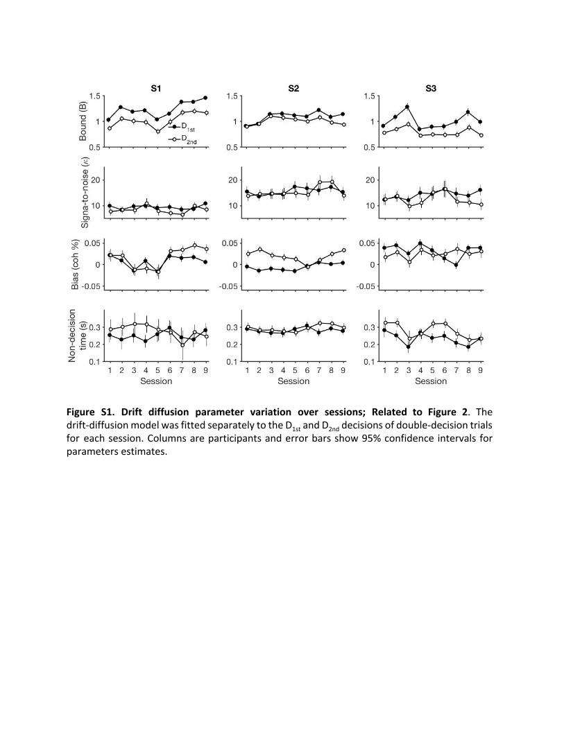
Figure S1. Drift diffusion parameter variation over sessions; Related to Figure 2. The drift-diffusion model was fitted separately to the D 1st and D 2nd decisions of double-decision trials for each session. Columns are participants and error bars show 95% confidence intervals for parameters estimates.

Figure S2. Correlation between reactions times on D 1st and D 2nd; Related to Figure 3. Reaction times were z-scored within each coherence and session. Also shown are 2-sd principal component ellipses. The correlations are significant for S1 (p<0.001) and S3 (p<0.001) but not for S2 (p=0.68).

Figure S3 Within vs. across trial effects of coherence on previous decision vs. reaction time on current decision; Related to Figure 3. The black data reproduces Figure 3B (top), showing RT on D 2nd and a function of coherence on D 1st . The blue data show across-trial effects, showing reaction time on first decision of a trial against the coherence of the last decision on the previous trial. Coherence of the preceding trial decision does not affect the RT of the current decision (p>0.19 for all three subjects). Error bars show s.e.m.
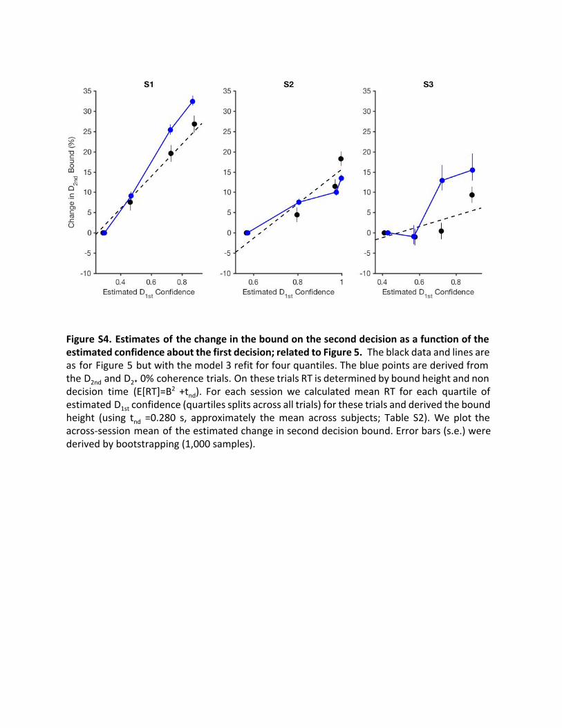
Figure S4. Estimates of the change in the bound on the second decision as a function of the estimated confidence about the first decision; related to Figure 5. The black data and lines are as for Figure 5 but with the model 3 refit for four quantiles. The blue points are derived from the D 2nd and D 2* 0% coherence trials. On these trials RT is determined by bound height and non decision time (E[RT]=B 2 +t nd ). For each session we calculated mean RT for each quartile of estimated D 1st confidence (quartiles splits across all trials) for these trials and derived the bound height (using tnd =0.280 s, approximately the mean across subjects; Table S2). We plot the across-session mean of the estimated change in second decision bound. Error bars (s.e.) were derived by bootstrapping (1,000 samples).
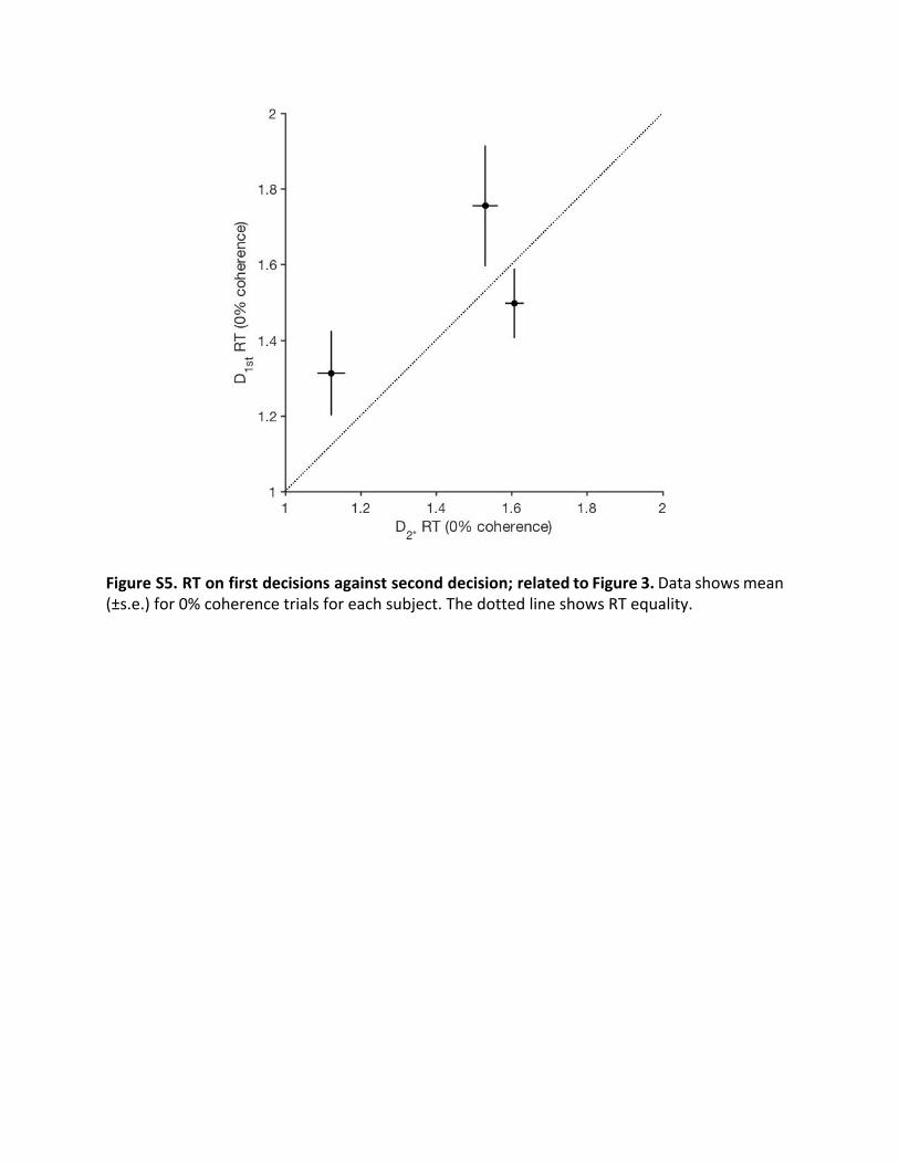
Figure S5. RT on first decisions against second decision; related to Figure 3. Data shows mean (±s.e.) for 0% coherence trials for each subject. The dotted line shows RT equality.

Table S1. Fitted parameters of the drift-diffusion model; related to Figure 2. The model was fit to single first decisions (D 1* ) and to the first of two decisions (D 1st including D 1st-catch trials). Parameter means are shown ±s.e. For simplicity bias (C 0) was set to zero.
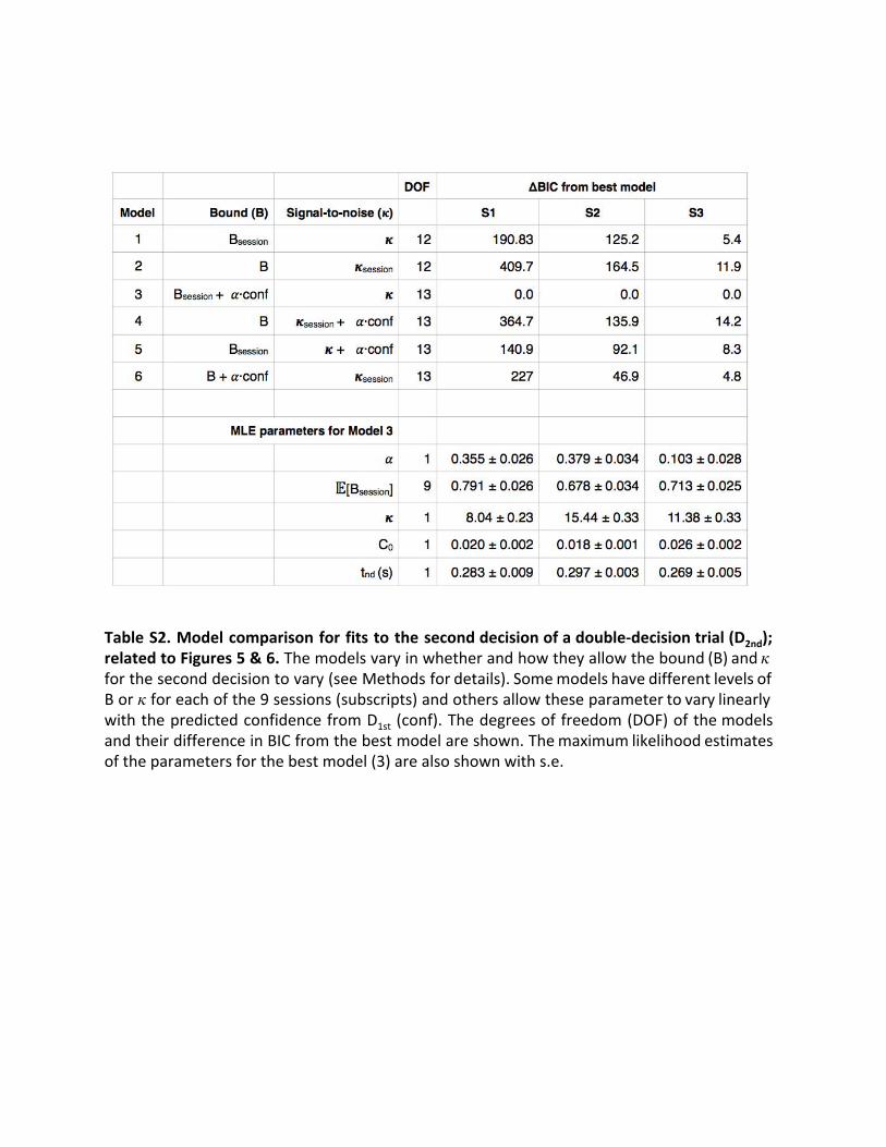
Table S2. Model comparison for fits to the second decision of a double-decision trial (D 2nd); related to Figures 5 & 6. The models vary in whether and how they allow the bound (B) and 𝜅 for the second decision to vary (see Methods for details). Some models have different levels of B or 𝜅 for each of the 9 sessions (subscripts) and others allow these parameter to vary linearly with the predicted confidence from D 1st (conf). The degrees of freedom (DOF) of the models and their difference in BIC from the best model are shown. The maximum likelihood estimates of the parameters for the best model (3) are also shown with s.e.
Supplemental Experimental Procedures Starting point vs. drift bias We accounted for possible biases by including a bias on drift in the model (the C 0 parameter).
However, there is some evidence suggesting that the locus of bias is instead in bound
asymmetries (Refs S1, S2) , (but see S3) which is equivalent to a starting point bias in our model.
We compared these alternatives by fitting all first choices that were part of a double decision
(D 1st ), with either a C 0 (coherence bias) term or y0 (offset bias) term. For all three subjects, the
model with C 0 bias was strongly preferred over the model with y0 (∆BIC is 21.8, 21.1, and 183.0
for subjects 1-3, respectively; same as deviance as d.f. are same), which justifies the assumption
in our main model. Note that S3 is the most informative subject as bias is small for S1 and S2.
We chose to fit with only C0 to reduce the number of parameters.
Normative model We used dynamic programming to determine the optimal decision policy for D 2nd as a function
of the confidence in D 1st . By optimal we refer to the decision policy that maximizes reward rate
(i.e., maximizing the number of points obtained per unit of time). The goal of this exercise is not
to establish that our participants were maximizing reward rate, but to justify their strategy as
sensible given a cost of time per trial.
The random dot motion discrimination task can be considered an instance of a class of
problems referred to as partially-observable Markov Decision Process (POMDP). The partial
observability derives from the fact that (motion) observations provide only ambiguous evidence
about the true underlying task state. Following the usual approach, we solve the POMDP
casting it as a fully observable Markov decision process (MDP) over the belief states of the
agent. We then use dynamic programming to find the policy that maximizes average reward.
Formally, an MDP can be described as a tuple given by (S4) :
(i) a non-empty state space ,S
(ii) an initial state ,S0
(iii) a goal state ,SG
(iv) a set of actions applicable in state ,(s)A s
(v) positive and negative rewards for doing action in state ,(a, )r s a s

(vi) transition probabilities indexing the probability of transitioning to state after (s |s)Pa ′ s′
doing action in state .a s
For simplicity, we derive the optimal policy for the second decision assuming that D 2nd is
informed by the confidence in D 1st , without explicitly modeling the decision process for the first
decision. Next, we describe how to cast the motion discrimination task as an MDP.
The state was defined as a tuple , where is the amount of accumulated motion s x, , ⟩⟨ t c1 x
evidence for one direction and against the other (the decision variable). It is positive when the
evidence supports one motion direction (say upwards), and negative when it supports the
opposite direction. is the elapsed decision time since the onset of motion for the second t
decision. is the probability that the first decision was correct. We assume that takes a c1 c1
value from the set , which corresponds respectively to the average confidence 0.6, .8, ]C1 = [ 0 1
for incorrect, correct and bypassed first decisions. This is a simplification because correct and
incorrect decisions are associated with a distribution of confidence values. However, we note
that our conclusions do not depend on this simplification as long as the average confidence
about D 1st is higher for correct than for error trials, which is indeed what was observed in our
data ( Figure 2 and 4). Further, we assume that the probability of eliciting each of the values in
was given by . Again, our conclusions are robust to changes in theseC1 0.3, .5, .2]pC1= [ 0 0
values. The decision process starts with (i.e., no accumulated evidence favoring either of the x = 0
alternatives), and . The distribution over was implemented with an initial state t = 0 ∈ Cc1 1 c1
that has transition probabilities to the three states .s0 pc1x , , ∈C ⟩⟨ = 0 t = 0 c1 1
Three actions were applicable in each state. The decision maker could either terminate the trial
by selecting one of the targets (two possible actions), or maintain fixation (the third ‘action’) to
gather additional motion evidence. Defining a deterministic policy entails specifying which
action to select in each state.
Transition probabilities indicate the probability of transitioning to after performing (s |s)Pa ′ s′
action in state . State transitions are not deterministic because they depend on the a s
momentary motion evidence, which is stochastic even if the motion coherence were known. As
in the bounded accumulation model, we assume that the momentary motion evidence follows
a normal distribution with a mean that depends linearly on motion coherence, such that over
one second of stimulus viewing the evidence accumulated is, on average, 𝜅. coh and the
variance of the momentary is equal to . For the analyses shown in Figure 7 we set 𝜅=10.1
For a given motion coherence, the probability of transitioning from state to state ⟨x, , ⟩s = t c1
is given by: ⟨x , t t, c ⟩s′ = ′ + δ 1
(1)
where is the normal p.d.f. with mean and standard deviation .(·|μ, )N σ μ σ
Because the decision-maker does not know the motion coherence with certainty, obtaining the
transition probability requires marginalizing over coherences: (s | s)pfix ′
(2)
This marginalization requires knowledge of , the probability that the underlying motion (coh|s)p
coherence is given that state was reached (S5) :ohc s
(3)
where the coherences are the discrete set of signed coherences used in the experiment, ohc
and is the normalization constant which assures that the sum of over all Z (coh|⟨x, , ⟩)p t c1
motion coherences adds to one. As in the experiment, is distributed uniformly over the (coh)p
discrete set of motion coherences.
We assume that the optimal decision-maker maximizes the reward per unit of time. To find the
optimal policy, we used value iteration to solve Bellman’s equation. For problems that have a
recurrent state—which includes decision-making tasks that are organized as a sequence of
trials—the problem of maximizing average reward can be recast as a stochastic shortest path
problem (or Goal MDP) through the inclusion of an artificial cost-free and absorbing goal state
(S4) . The intuition behind this simplification is that if we consider a sequence of generated

trajectories in state space, we can divide it into a series of visits to the recurrent state, which is
equivalent to the corresponding Goal MDP where the recurrent state is the goal state (S4) .
For our task, the Bellman equation takes the form:
(4)
where are states and is the average non-decision time. The time is the average , ss ′ tnd tother
time gap between a response to D 2nd and the onset of motion for the following D 2nd ; it includes
the time spent on fixations, reporting confidence, responding to the first decision, receiving
feedback, etc. For the analyses of Figure 7, we chose and . is the .3 stnd = 0 stother = 5 Rc
reward obtained after a correct response, and is the reward obtained after an incorrect Rnc
response. As in the experiment, and . Reward rate is the reward obtained per Rc = 1 Rnc = 0 ρ
unit of time.
is the probability of being correct after doing action in state . For the double decision(s)pc|a a s
trials, being correct means solving both decisions correctly. Therefore, is the probability (s)pc|a
that the first decision was correct ( ) , multiplied by the probability that D 2nd was solved c1
correctly. The latter can be obtained summing over the coherences for which the action is a
the appropriate action. For instance, the action ‘up’ is the appropriate action for all positive and
for half of the 0% coherence trials. Therefore
(5)
Our depiction of Bellman’s equation implicitly assumes that choosing a terminal action leads to
an absorbing cost-free state. The expectation in is an expectation over all future states (s, ix)Q f
that result from being in and gathering evidence for an additional time step :s′ s tδ
(6)
Because time flows in a single direction, Bellman’s equation can be solved by backwards
induction in a single pass. However, since we want to maximize the reward rate, which depends
on the policy itself, we perform multiple backwards passes to find the value of through ρ
root-finding, bracketing within a sequence of diminishing intervals until the value of the ρ
initial state is approximately zero (S4, S6) .(S )V 0
Supplemental References
S1. White, C. N., and Poldrack, R. A. (2014) Decomposing bias in different types of simple
decisions. J. Exp. Psychol. Learn. Mem. Cogn. 40, 385–398
S2. van Ravenzwaaij, D., Mulder, M. J., Tuerlinckx, F., and Wagenmakers, E.-J. (2012) Do the
dynamics of prior information depend on task context? An analysis of optimal
performance and an empirical test. Front. Psychol. 3, 132
S3. Moran, R. (2015) Optimal decision making in heterogeneous and biased environments.
Psychon. Bull. Rev. 22, 38–53
S4. Bertsekas, D. P. (1995) Dynamic programming and optimal control (Athena Scientific,
Belmont, MA)
S5. Moreno-Bote, R. (2010) Decision confidence and uncertainty in diffusion models with
partially correlated neuronal integrators. Neural Comput. 22, 1786–1811
S6. Drugowitsch, J., Moreno-Bote, R., Churchland, A. K., Shadlen, M. N., and Pouget, A. (2012)
The cost of accumulating evidence in perceptual decision making. J. Neurosci. 32,
3612–3628
Current Biology, Volume 26
Supplemental Information
Confidence Is the Bridge
between Multi-stage Decisions
Ronald van den Berg, Ariel Zylberberg, Roozbeh Kiani, Michael N. Shadlen, and Daniel M.Wolpert

Figure S1. Drift diffusion parameter variation over sessions; Related to Figure 2. The drift-diffusion model was fitted separately to the D 1st and D 2nd decisions of double-decision trials for each session. Columns are participants and error bars show 95% confidence intervals for parameters estimates.
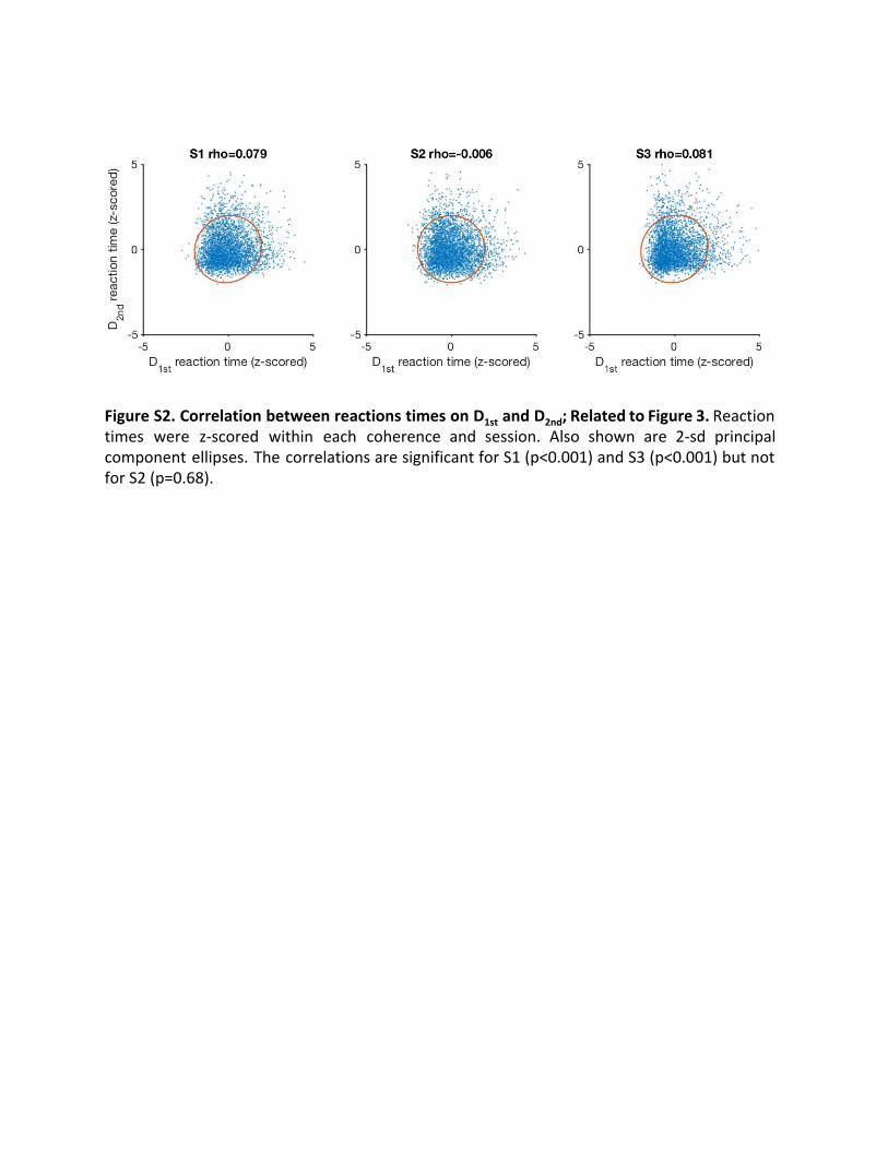
Figure S2. Correlation between reactions times on D 1st and D 2nd; Related to Figure 3. Reaction times were z-scored within each coherence and session. Also shown are 2-sd principal component ellipses. The correlations are significant for S1 (p<0.001) and S3 (p<0.001) but not for S2 (p=0.68).
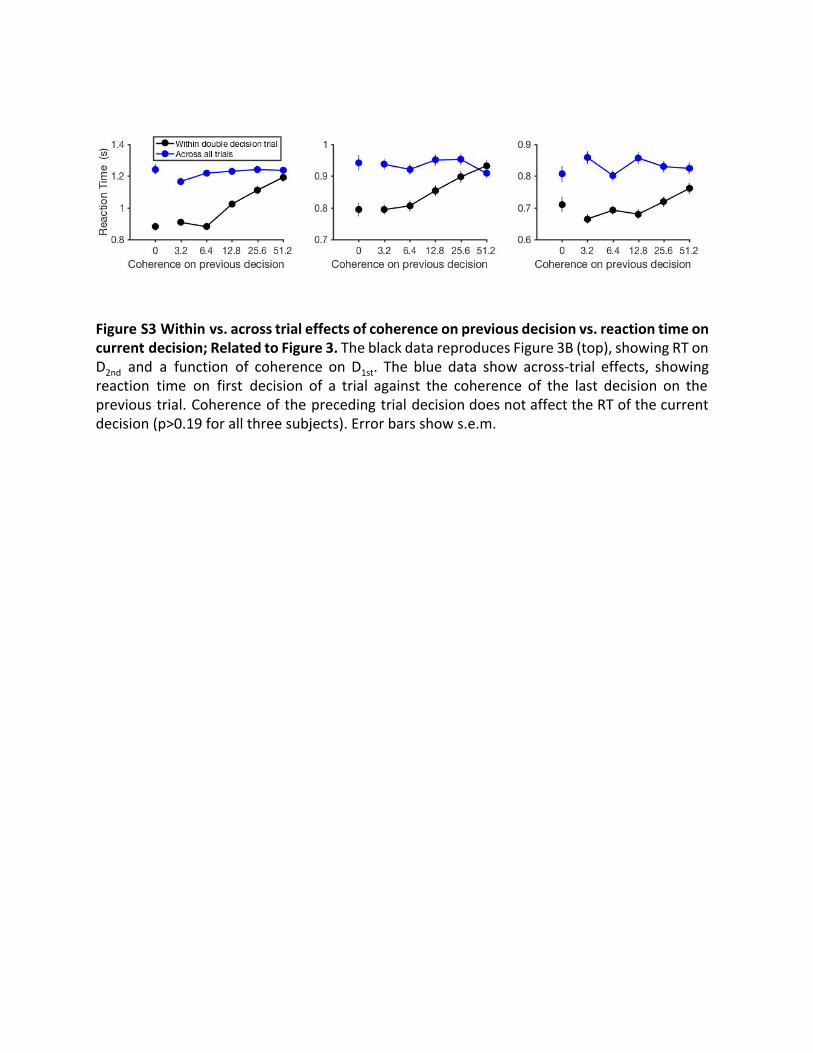
Figure S3 Within vs. across trial effects of coherence on previous decision vs. reaction time on current decision; Related to Figure 3. The black data reproduces Figure 3B (top), showing RT on D 2nd and a function of coherence on D 1st . The blue data show across-trial effects, showing reaction time on first decision of a trial against the coherence of the last decision on the previous trial. Coherence of the preceding trial decision does not affect the RT of the current decision (p>0.19 for all three subjects). Error bars show s.e.m.

Figure S4. Estimates of the change in the bound on the second decision as a function of the estimated confidence about the first decision; related to Figure 5. The black data and lines are as for Figure 5 but with the model 3 refit for four quantiles. The blue points are derived from the D 2nd and D 2* 0% coherence trials. On these trials RT is determined by bound height and non decision time (E[RT]=B 2 +t nd ). For each session we calculated mean RT for each quartile of estimated D 1st confidence (quartiles splits across all trials) for these trials and derived the bound height (using tnd =0.280 s, approximately the mean across subjects; Table S2). We plot the across-session mean of the estimated change in second decision bound. Error bars (s.e.) were derived by bootstrapping (1,000 samples).

Figure S5. RT on first decisions against second decision; related to Figure 3. Data shows mean (±s.e.) for 0% coherence trials for each subject. The dotted line shows RT equality.
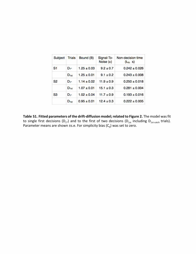
Table S1. Fitted parameters of the drift-diffusion model; related to Figure 2. The model was fit to single first decisions (D 1* ) and to the first of two decisions (D 1st including D 1st-catch trials). Parameter means are shown ±s.e. For simplicity bias (C 0) was set to zero.

Table S2. Model comparison for fits to the second decision of a double-decision trial (D 2nd); related to Figures 5 & 6. The models vary in whether and how they allow the bound (B) and 𝜅 for the second decision to vary (see Methods for details). Some models have different levels of B or 𝜅 for each of the 9 sessions (subscripts) and others allow these parameter to vary linearly with the predicted confidence from D 1st (conf). The degrees of freedom (DOF) of the models and their difference in BIC from the best model are shown. The maximum likelihood estimates of the parameters for the best model (3) are also shown with s.e.

Supplemental Experimental Procedures Starting point vs. drift bias We accounted for possible biases by including a bias on drift in the model (the C 0 parameter).
However, there is some evidence suggesting that the locus of bias is instead in bound
asymmetries (Refs S1, S2) , (but see S3) which is equivalent to a starting point bias in our model.
We compared these alternatives by fitting all first choices that were part of a double decision
(D 1st ), with either a C 0 (coherence bias) term or y0 (offset bias) term. For all three subjects, the
model with C 0 bias was strongly preferred over the model with y0 (∆BIC is 21.8, 21.1, and 183.0
for subjects 1-3, respectively; same as deviance as d.f. are same), which justifies the assumption
in our main model. Note that S3 is the most informative subject as bias is small for S1 and S2.
We chose to fit with only C0 to reduce the number of parameters.
Normative model We used dynamic programming to determine the optimal decision policy for D 2nd as a function
of the confidence in D 1st . By optimal we refer to the decision policy that maximizes reward rate
(i.e., maximizing the number of points obtained per unit of time). The goal of this exercise is not
to establish that our participants were maximizing reward rate, but to justify their strategy as
sensible given a cost of time per trial.
The random dot motion discrimination task can be considered an instance of a class of
problems referred to as partially-observable Markov Decision Process (POMDP). The partial
observability derives from the fact that (motion) observations provide only ambiguous evidence
about the true underlying task state. Following the usual approach, we solve the POMDP
casting it as a fully observable Markov decision process (MDP) over the belief states of the
agent. We then use dynamic programming to find the policy that maximizes average reward.
Formally, an MDP can be described as a tuple given by (S4) :
(i) a non-empty state space ,S
(ii) an initial state ,S0
(iii) a goal state ,SG
(iv) a set of actions applicable in state ,(s)A s
(v) positive and negative rewards for doing action in state ,(a, )r s a s
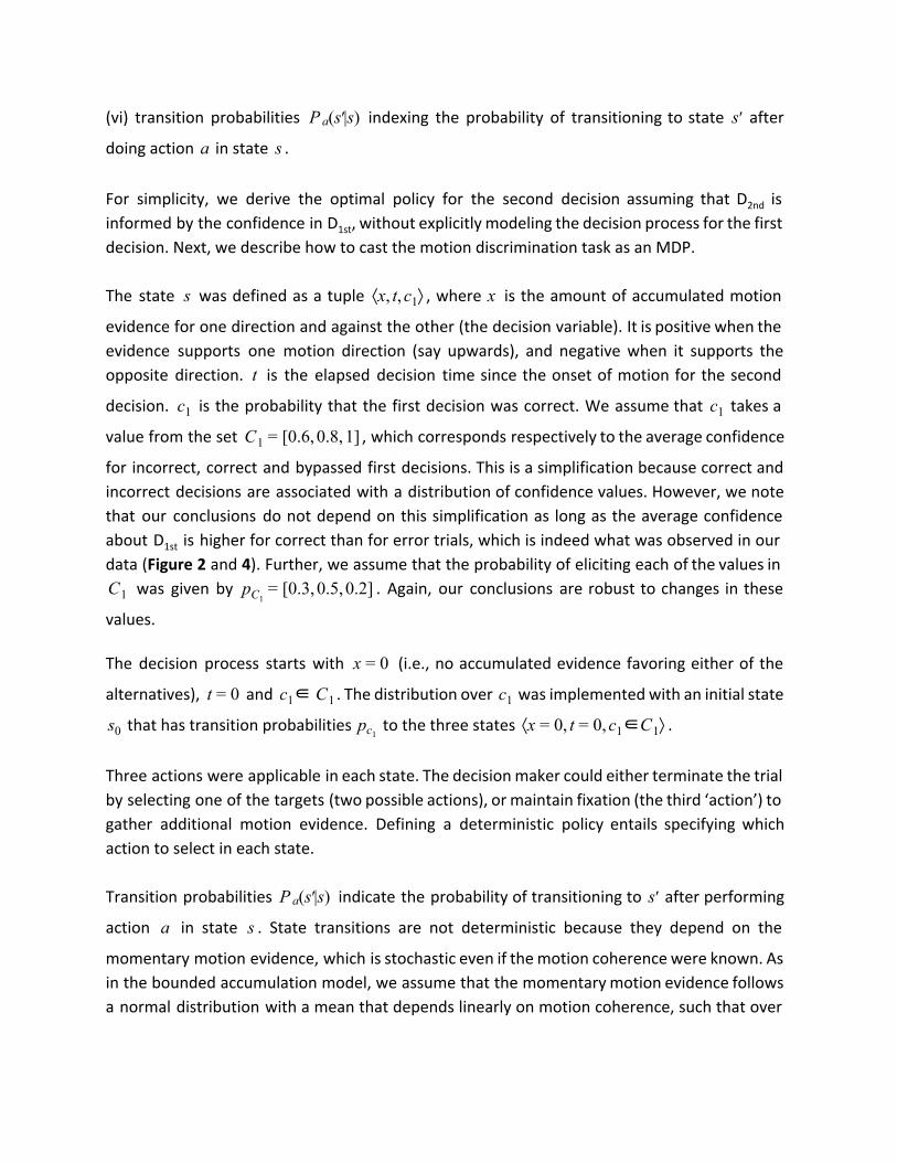
(vi) transition probabilities indexing the probability of transitioning to state after (s |s)Pa ′ s′
doing action in state .a s
For simplicity, we derive the optimal policy for the second decision assuming that D 2nd is
informed by the confidence in D 1st , without explicitly modeling the decision process for the first
decision. Next, we describe how to cast the motion discrimination task as an MDP.
The state was defined as a tuple , where is the amount of accumulated motion s x, , ⟩⟨ t c1 x
evidence for one direction and against the other (the decision variable). It is positive when the
evidence supports one motion direction (say upwards), and negative when it supports the
opposite direction. is the elapsed decision time since the onset of motion for the second t
decision. is the probability that the first decision was correct. We assume that takes a c1 c1
value from the set , which corresponds respectively to the average confidence 0.6, .8, ]C1 = [ 0 1
for incorrect, correct and bypassed first decisions. This is a simplification because correct and
incorrect decisions are associated with a distribution of confidence values. However, we note
that our conclusions do not depend on this simplification as long as the average confidence
about D 1st is higher for correct than for error trials, which is indeed what was observed in our
data ( Figure 2 and 4). Further, we assume that the probability of eliciting each of the values in
was given by . Again, our conclusions are robust to changes in theseC1 0.3, .5, .2]pC1= [ 0 0
values. The decision process starts with (i.e., no accumulated evidence favoring either of the x = 0
alternatives), and . The distribution over was implemented with an initial state t = 0 ∈ Cc1 1 c1
that has transition probabilities to the three states .s0 pc1x , , ∈C ⟩⟨ = 0 t = 0 c1 1
Three actions were applicable in each state. The decision maker could either terminate the trial
by selecting one of the targets (two possible actions), or maintain fixation (the third ‘action’) to
gather additional motion evidence. Defining a deterministic policy entails specifying which
action to select in each state.
Transition probabilities indicate the probability of transitioning to after performing (s |s)Pa ′ s′
action in state . State transitions are not deterministic because they depend on the a s
momentary motion evidence, which is stochastic even if the motion coherence were known. As
in the bounded accumulation model, we assume that the momentary motion evidence follows
a normal distribution with a mean that depends linearly on motion coherence, such that over

one second of stimulus viewing the evidence accumulated is, on average, 𝜅. coh and the
variance of the momentary is equal to . For the analyses shown in Figure 7 we set 𝜅=10.1
For a given motion coherence, the probability of transitioning from state to state ⟨x, , ⟩s = t c1
is given by: ⟨x , t t, c ⟩s′ = ′ + δ 1
(1)
where is the normal p.d.f. with mean and standard deviation .(·|μ, )N σ μ σ
Because the decision-maker does not know the motion coherence with certainty, obtaining the
transition probability requires marginalizing over coherences: (s | s)pfix ′
(2)
This marginalization requires knowledge of , the probability that the underlying motion (coh|s)p
coherence is given that state was reached (S5) :ohc s
(3)
where the coherences are the discrete set of signed coherences used in the experiment, ohc
and is the normalization constant which assures that the sum of over all Z (coh|⟨x, , ⟩)p t c1
motion coherences adds to one. As in the experiment, is distributed uniformly over the (coh)p
discrete set of motion coherences.
We assume that the optimal decision-maker maximizes the reward per unit of time. To find the
optimal policy, we used value iteration to solve Bellman’s equation. For problems that have a
recurrent state—which includes decision-making tasks that are organized as a sequence of
trials—the problem of maximizing average reward can be recast as a stochastic shortest path
problem (or Goal MDP) through the inclusion of an artificial cost-free and absorbing goal state
(S4) . The intuition behind this simplification is that if we consider a sequence of generated
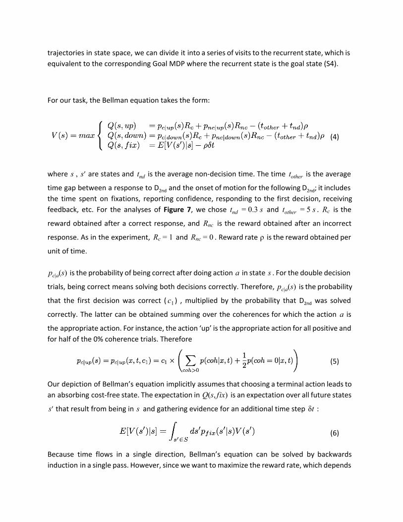
trajectories in state space, we can divide it into a series of visits to the recurrent state, which is
equivalent to the corresponding Goal MDP where the recurrent state is the goal state (S4) .
For our task, the Bellman equation takes the form:
(4)
where are states and is the average non-decision time. The time is the average , ss ′ tnd tother
time gap between a response to D 2nd and the onset of motion for the following D 2nd ; it includes
the time spent on fixations, reporting confidence, responding to the first decision, receiving
feedback, etc. For the analyses of Figure 7, we chose and . is the .3 stnd = 0 stother = 5 Rc
reward obtained after a correct response, and is the reward obtained after an incorrect Rnc
response. As in the experiment, and . Reward rate is the reward obtained per Rc = 1 Rnc = 0 ρ
unit of time.
is the probability of being correct after doing action in state . For the double decision(s)pc|a a s
trials, being correct means solving both decisions correctly. Therefore, is the probability (s)pc|a
that the first decision was correct ( ) , multiplied by the probability that D 2nd was solved c1
correctly. The latter can be obtained summing over the coherences for which the action is a
the appropriate action. For instance, the action ‘up’ is the appropriate action for all positive and
for half of the 0% coherence trials. Therefore
(5)
Our depiction of Bellman’s equation implicitly assumes that choosing a terminal action leads to
an absorbing cost-free state. The expectation in is an expectation over all future states (s, ix)Q f
that result from being in and gathering evidence for an additional time step :s′ s tδ
(6)
Because time flows in a single direction, Bellman’s equation can be solved by backwards
induction in a single pass. However, since we want to maximize the reward rate, which depends

on the policy itself, we perform multiple backwards passes to find the value of through ρ
root-finding, bracketing within a sequence of diminishing intervals until the value of the ρ
initial state is approximately zero (S4, S6) .(S )V 0
Supplemental References
S1. White, C. N., and Poldrack, R. A. (2014) Decomposing bias in different types of simple
decisions. J. Exp. Psychol. Learn. Mem. Cogn. 40, 385–398
S2. van Ravenzwaaij, D., Mulder, M. J., Tuerlinckx, F., and Wagenmakers, E.-J. (2012) Do the
dynamics of prior information depend on task context? An analysis of optimal
performance and an empirical test. Front. Psychol. 3, 132
S3. Moran, R. (2015) Optimal decision making in heterogeneous and biased environments.
Psychon. Bull. Rev. 22, 38–53
S4. Bertsekas, D. P. (1995) Dynamic programming and optimal control (Athena Scientific,
Belmont, MA)
S5. Moreno-Bote, R. (2010) Decision confidence and uncertainty in diffusion models with
partially correlated neuronal integrators. Neural Comput. 22, 1786–1811
S6. Drugowitsch, J., Moreno-Bote, R., Churchland, A. K., Shadlen, M. N., and Pouget, A. (2012)
The cost of accumulating evidence in perceptual decision making. J. Neurosci. 32,
3612–3628