confronting theory with observations workshop, nbia, copenhagen, august 18, 20101 analysing the cmb...

Confronting theory with observations workshop, NBIA, Copenhagen, August 18, 2010 1

Analysing the CMBin a model-independent

manner

Analysing the CMBin a model-independent

manner

Syksy Räsänen

University of Helsinki

Syksy Räsänen

University of Helsinki

JCAP08(2010)023, arXiv:1003.0810(M. Vonlanthen, SR and R. Durrer)

JCAP08(2010)023, arXiv:1003.0810(M. Vonlanthen, SR and R. Durrer)


Model-dependenceModel-dependence Usually in CMB analysis, a specific model is assumed for

both the early and the late universe, and their physics is not disentangled.

Limits on early parameters such as ωm and ns have an unquantified dependence on the late universe model.

On the other hand, constraints are quoted on parameters such as spatial curvature or H0, to which the CMB has no direct sensitivity.

Usually in CMB analysis, a specific model is assumed for both the early and the late universe, and their physics is not disentangled.

Limits on early parameters such as ωm and ns have an unquantified dependence on the late universe model.

On the other hand, constraints are quoted on parameters such as spatial curvature or H0, to which the CMB has no direct sensitivity.


Physics probed by the CMBPhysics probed by the CMB The observed CMB anisotropies depend on

1) The pattern set at decoupling and 2) The processing between decoupling and today.

The initial pattern is given by well understood atomic and gravitational physics at last scattering (and the seeds of structure).

Late evolution involves reionisation, as well as poorly understood physics of late universe (dark energy, modified gravity, non-linearities).

We keep 1) fixed, and remain agnostic about 2).

The observed CMB anisotropies depend on 1) The pattern set at decoupling and 2) The processing between decoupling and today.

The initial pattern is given by well understood atomic and gravitational physics at last scattering (and the seeds of structure).

Late evolution involves reionisation, as well as poorly understood physics of late universe (dark energy, modified gravity, non-linearities).

We keep 1) fixed, and remain agnostic about 2).


The CMB parametersThe CMB parameters Keeping general relativity, atomic physics and CDM fixed,

the decoupling pattern is set by 1) the baryon density ωb,

2) the CDM density ωc and, 3) the primordial spectral index ns and amplitude A.

Late evolution changes 1) the overall amplitude, 2) the angular size, and 3) the subhorizon pattern

Keeping general relativity, atomic physics and CDM fixed, the decoupling pattern is set by 1) the baryon density ωb,

2) the CDM density ωc and, 3) the primordial spectral index ns and amplitude A.

Late evolution changes 1) the overall amplitude, 2) the angular size, and 3) the subhorizon pattern

⇒ Marginalise ⇒ Parametrise

⇒ Cut

⇒ Marginalise ⇒ Parametrise

⇒ Cut


Angular sizeAngular size

The angular size is given by DA = L/θ.

In the flat sky approximation, this reduces to .

Taking the Einstein-de Sitter model as comparison,we have , where .

The angular size is given by DA = L/θ.

In the flat sky approximation, this reduces to .

Taking the Einstein-de Sitter model as comparison,we have , where .

€

C(θ) ≡ ΔT(n1)ΔT(n2) =1

4π(2l +1)

l∑ Cl Pl (cosθ) =

1

4π(2l +1)

l∑ ′ C l Pl (cos ′ θ )

€

Cl =1

4π

(2 ′ l +1)

2(2 ′ l +1)

′ l ∑ ′ C ′ l sin

0

π

∫ θdθP ′ l cos θDA

′ D A

⎛

⎝ ⎜

⎞

⎠ ⎟

⎡

⎣ ⎢

⎤

⎦ ⎥ Pl (cosθ)

€

C(r) =1

2πdll

0

∞

∫ J0(rl )Cl

€

Cl =′ D A

DA

⎛

⎝ ⎜

⎞

⎠ ⎟

2

′ C ′ D ADA

′ l ⇒

⇒

€

Cl = S−2CS −1 ′ l

EdS

€

S ≡DA

DAEdS


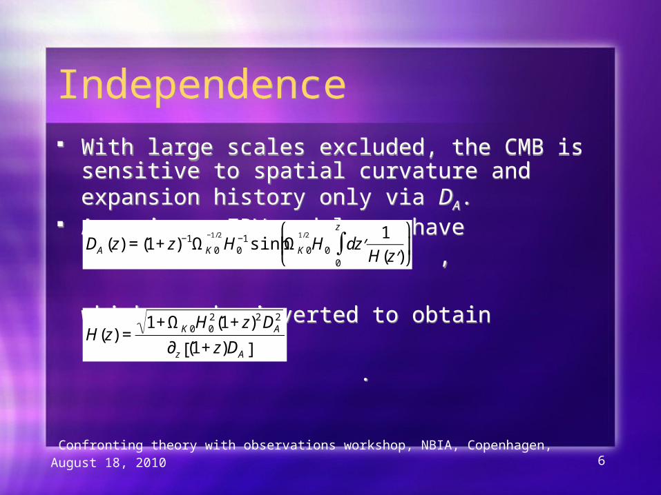
IndependenceIndependence With large scales excluded, the CMB is sensitive to spatial

curvature and expansion history only via DA. Assuming a FRW model, we have

,

which can be inverted to obtain

.

With large scales excluded, the CMB is sensitive to spatial curvature and expansion history only via DA.

Assuming a FRW model, we have ,

which can be inverted to obtain

.€

DA (z) = (1+ z)−1ΩK 0

−1/2

H0−1 sinh ΩK 0

1/2

H0 d ′ z 1

H( ′ z )0

z

∫ ⎛

⎝ ⎜

⎞

⎠ ⎟

€

H(z) =1+ ΩK 0H0

2(1+ z)2 DA2

∂z (1+ z)DA[ ]


Cutting large scalesCutting large scales Causal physics can change the correlation properties on

subhorizon scales. The effects (ISW, RS, SZ, lensing, ...) are model-

dependent. The physics at late times is unknown, so we drop low

multipoles. From FRW+linear models of reionisation and the ISW

effect, we know that we should cut to at least l =20-40. We do not take into account gravity waves, vectors or

neutrino masses.

Causal physics can change the correlation properties on subhorizon scales.

The effects (ISW, RS, SZ, lensing, ...) are model-dependent.

The physics at late times is unknown, so we drop low multipoles.

From FRW+linear models of reionisation and the ISW effect, we know that we should cut to at least l =20-40.

We do not take into account gravity waves, vectors or neutrino masses.


Varying the cutVarying the cut Fitting ΛCDM to ACBAR and WMAP5, we get (τ = 0)

From lmin= 2 to lmin= 40, the errors on ωb and ωc grow by 28% and on ns by 57%, while the means shift by 1%, 4% and 1%.

Fitting ΛCDM to ACBAR and WMAP5, we get (τ = 0)

From lmin= 2 to lmin= 40, the errors on ωb and ωc grow by 28% and on ns by 57%, while the means shift by 1%, 4% and 1%.


A systematic shiftA systematic shift

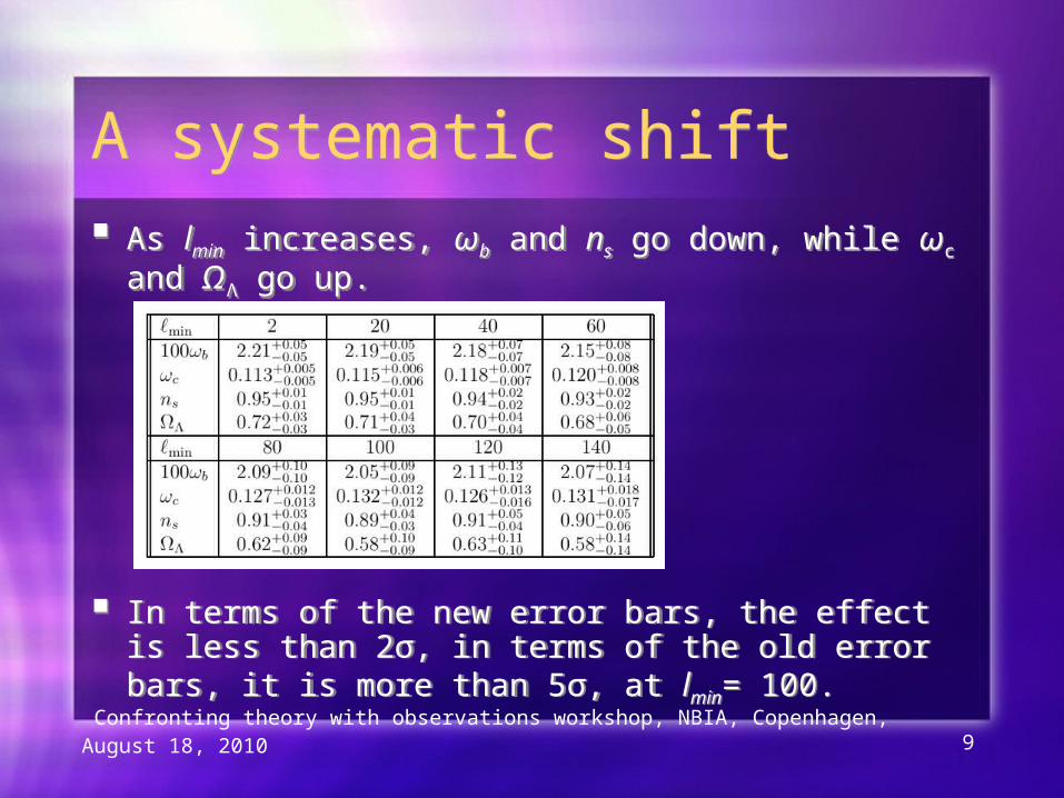
As lmin increases, ωb and ns go down, while ωc and ΩΛ go up.

In terms of the new error bars, the effect is less than 2σ, in terms of the old error bars, it is more than 5σ, at lmin= 100.

As lmin increases, ωb and ns go down, while ωc and ΩΛ go up.

In terms of the new error bars, the effect is less than 2σ, in terms of the old error bars, it is more than 5σ, at lmin= 100.


Large angle amplitudeLarge angle amplitude The shift corresponds to increasing low multipole power: The shift corresponds to increasing low multipole power:


Shifted resultsShifted results

We fix the cut at lmin= 40, corresponding to z ≾60. The mean values change more than the error bars. The angle θA = rs/DA is stable and determined to 0.3%.

We fix the cut at lmin= 40, corresponding to z ≾60. The mean values change more than the error bars. The angle θA = rs/DA is stable and determined to 0.3%.


SummarySummary

The values of ωb, ωc, ns and θA are determined by the CMB to a precision of 3%, 6%, 2% and 0.3%.

However, a systematic shift affects all parameters except θA.

The small-angle CMB sky prefers different values of ωb, ωc, ns than the full dataset.

It would be interesting to analyse BAO in the same model-independent spirit.

The values of ωb, ωc, ns and θA are determined by the CMB to a precision of 3%, 6%, 2% and 0.3%.

However, a systematic shift affects all parameters except θA.

The small-angle CMB sky prefers different values of ωb, ωc, ns than the full dataset.

It would be interesting to analyse BAO in the same model-independent spirit.

confronting theory with observations workshop, nbia, copenhagen, august 18, 20101 analysing the cmb...

Documents