connecting machine learning with shallow neural networks · 2018-05-19 · the deep learning...

Charu C. Aggarwal

IBM T J Watson Research Center

Yorktown Heights, NY

Connecting Machine Learning with Shallow

Neural Networks

Neural Networks and Deep Learning, Springer, 2018

Chapter 2, Section 2.1

Neural Networks and Machine Learning

• Neural networks are optimization-based learning models.

• Many classical machine learning models use continuous op-

timization:

– SVMs, Linear Regression, and Logistic Regression

– Singular Value Decomposition

– (Incomplete) Matrix factorization for Recommender Sys-

tems

• All these models can be represented as special cases of shal-

low neural networks!

The Continuum Between Machine Learning and Deep

Learning

ACCU

RACY

AMOUNT OF DATA

DEEP LEARNING

CONVENTIONALMACHINE LEARNING

• Classical machine learning models reach their learning capac-

ity early because they are simple neural networks.

• When we have more data, we can add more computational

units to improve performance.

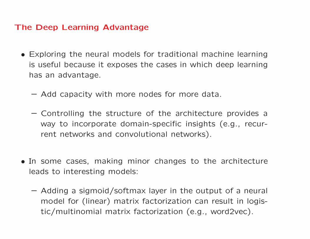
The Deep Learning Advantage

• Exploring the neural models for traditional machine learning

is useful because it exposes the cases in which deep learning

has an advantage.

– Add capacity with more nodes for more data.

– Controlling the structure of the architecture provides a

way to incorporate domain-specific insights (e.g., recur-

rent networks and convolutional networks).

• In some cases, making minor changes to the architecture

leads to interesting models:

– Adding a sigmoid/softmax layer in the output of a neural

model for (linear) matrix factorization can result in logis-

tic/multinomial matrix factorization (e.g., word2vec).

Recap: Perceptron versus Linear Support Vector Machine

∑ OUTPUT NODE

y LOSS = MAX(0,-y[W X])

LINEAR ACTIVATION

PERCEPTRON CRITERION (SMOOTH SURROGATE)

X

INPUT NODES W

∑ OUTPUT NODE

y LOSS = MAX(0,-y[W X]+1)

LINEAR ACTIVATION

HINGE LOSS

X

INPUT NODES W

(a) Perceptron (b) SVMLoss = max{0,−y(W ·X)} Loss = max{0,1− y(W ·X)}

• The Perceptron criterion is a minor variation of hinge loss

with identical update of W ⇐ W + αyX in both cases.

• We update only for misclassified instances in perceptron, but

update also for “marginally correct” instances in SVM.

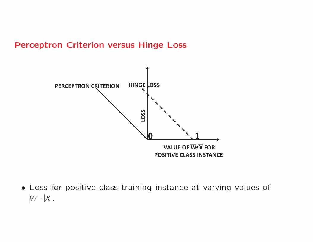
Perceptron Criterion versus Hinge Loss

LOSS

PERCEPTRON CRITERION HINGE LOSS

10VALUE OF W X FOR

POSITIVE CLASS INSTANCE

• Loss for positive class training instance at varying values of

W ·X.

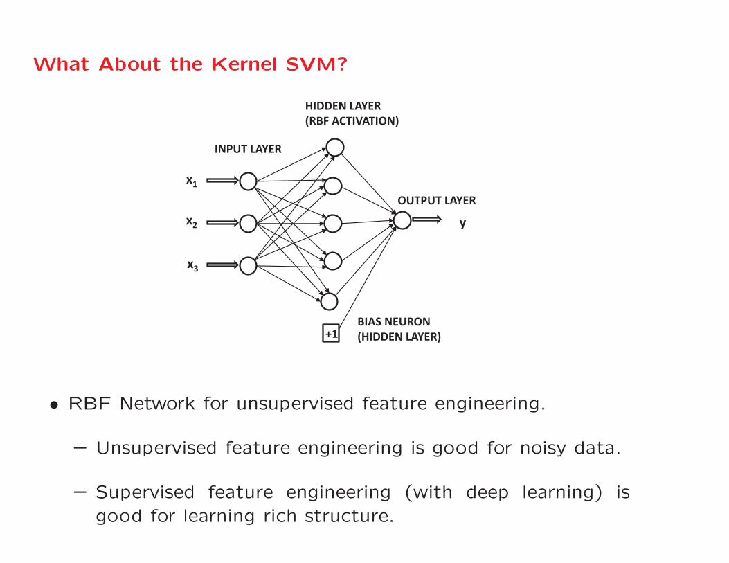
What About the Kernel SVM?

INPUT LAYER

HIDDEN LAYER (RBF ACTIVATION)

OUTPUT LAYER

y

x3

x2

x1

+1BIAS NEURON(HIDDEN LAYER)

• RBF Network for unsupervised feature engineering.

– Unsupervised feature engineering is good for noisy data.

– Supervised feature engineering (with deep learning) isgood for learning rich structure.

Much of Machine Learning is a Shallow Neural Model

• By minor changes to the architecture of perceptron we canget:

– Linear regression, Fisher discriminant, and Widrow-Hofflearning ⇒ Linear activation in output node

– Logistic regression ⇒ Sigmoid activation in output node

• Multinomial logistic regression ⇒ Softmax Activation in FinalLayer

• Singular value decomposition ⇒ Linear autoencoder

• Incomplete matrix factorization for Recommender Systems⇒ Autoencoder-like architecture with single hidden layer(also used in word2vec)

Why do We Care about Connections?

• Connections tell us about the cases that it makes sense to

use conventional machine learning:

– If you have less data with noise, you want to use conven-

tional machine learning.

– If you have a lot of data with rich structure, you want to

use neural networks.

– Structure is often learned by using deep neural architec-

tures.

• Architectures like convolutional neural networks can use

domain-specific insights.

Charu C. Aggarwal



Neural Models for Linear Regression,

Classification, and the Fisher Discriminant

[Connections with Widrow-Hoff Learning]



Widrow-Hoff Rule: The Neural Avatar of LinearRegression

• The perceptron (1958) was historically followed by Widrow-Hoff Learning (1960).

• Identical to linear regression when applied to numerical tar-gets.

– Originally proposed by Widrow and Hoff for binary targets(not natural for regression).

• The Widrow-Hoff method, when applied to mean-centeredfeatures and mean-centered binary class encoding, learns theFisher discriminant.

• We first discuss linear regression for numeric classes and thenvisit the case of binary classes.

Linear Regression: An Introduction

• In linear regression, we have training pairs (Xi, yi) for i ∈{1 . . . n}, so that Xi contains d-dimensional features and yicontains a numerical target.

• We use a linear parameterized function to predict yi = W ·Xi.

• Goal is to learn W , so that the sum-of-squared differencesbetween observed yi and predicted yi is minimized over theentire training data.

• Solution exists in closed form, but requires the inversion ofa potentially large matrix.

• Gradient-descent is typically used anyway.

Linear Regression with Numerical Targets:Neural Model

∑ OUTPUT NODE

y

LINEAR ACTIVATION

SQUARED LOSS

LOSS = (y-[W X])2 X

INPUT NODES W

• Predicted output is yi = W ·Xi and loss is Li = (yi − yi)2.

• Gradient-descent update is W ⇐ W−α∂Li∂W

= W+α(yi−yi)Xi.

Widrow-Hoff: Linear Regression with Binary Targets

• For yi ∈ {−1,+1}, we use same loss of (yi− yi)2, and update

of W ⇐ W + α (yi − yi)︸︷︷︸delta

Xi.

– When applied to binary targets, it is referred to as deltarule.

– Perceptron uses the same update with yi = sign{W ·Xi},whereas Widrow-Hoff uses yi = W ·Xi.

• Potential drawback: Retrogressive treatment of well-separated points caused by the pretension that binary targetsare real-valued.

– If yi = +1, and W · Xi = 106, the point will be heavilypenalized for strongly correct classification!

– Does not happen in perceptron.

Comparison of Widrow-Hoff with Perceptron and SVM

• Convert the binary loss functions and updates to a form more

easily comparable to perceptron using y2i = 1:

• Loss of (Xi, yi) is (yi −W ·Xi)2 = (1− yi[W ·Xi])

2

Update: W ⇐ W + αyi(1− yi[W ·Xi])Xi

Perceptron L1-Loss SVMLoss max{−yi(W ·Xi),0} max{1− yi(W ·Xi),0}

Update W ⇐ W + αyiI(−yi[W ·Xi] > 0)Xi W ⇐ W + αyiI(1− yi[W ·Xi] > 0)Xi

Widrow-Hoff Hinton’s L2-Loss SVMLoss (1− yi(W ·Xi))2 max{1− yi(W ·Xi),0}2

Update W ⇐ W + αyi(1− yi[W ·Xi])Xi W ⇐ W + αyimax{(1− yi[W ·Xi]),0}Xi

Some Interesting Historical Facts

• Hinton proposed the SVM L2-loss three years before Cortes

and Vapnik’s paper on SVMs.

– G. Hinton. Connectionist learning procedures. Artificial

Intelligence, 40(1–3), pp. 185–234, 1989.

– Hinton’s L2-loss was proposed to address some of the

weaknesses of loss functions like linear regression on binary

targets.

– When used with L2-regularization, it behaves identically to

an L2-SVM, but the connection with SVM was overlooked.

• The Widrow-Hoff rule is also referred to as ADALINE, LMS

(least mean-square method), delta rule, and least-squares

classification.

Connections with Fisher Discriminant

• Consider a binary classification problem with training in-

stances (Xi, yi) and yi ∈ {−1,+1}.

– Mean-center each feature vector as Xi − μ.

– Mean-center the binary class by subtracting∑n

i=1 yi/n

from each yi.

• Use the delta rule W ⇐ W + α (yi − yi)︸︷︷︸delta

Xi for learning.

• Learned vector is the Fisher discriminant!

– Proof in Christopher Bishop’s book on machine learning.

Charu C. Aggarwal



Neural Models for Logistic Regression



Logistic Regression: A Probabilistic Model

• Consider the training pair (Xi, yi) with d-dimensional featurevariables in Xi and class variable yi ∈ {−1,+1}.

• In logistic regression, the sigmoid function is applied to W ·Xi,which predicts the probability that yi is +1.

yi = P(yi = 1) =1

1+ exp(−W ·Xi)

• We want to maximize yi for positive class instances and 1− yifor negative class instances.

– Same as minimizing −log(yi) for positive class instancesand −log(1− yi) for negative instances.

– Same as minimizing loss Li = −log(|yi/2− 0.5 + yi|).

– Alternative form of loss Li = log(1+ exp[−yi(W ·Xi)])

Maximum-Likelihood Objective Functions

• Why did we use the negative logarithms?

• Logistic regression is an example of a maximum-likelihood

objective function.

• Our goal is to maximize the product of the probabilities of

correct classification over all training instances.

– Same as minimizing the sum of the negative log probabil-

ities.

– Loss functions are always additive over training instances.

– So we are really minimizing∑

i−log(|yi/2−0.5+ yi|) which

can be shown to be∑

i log(1 + exp[−yi(W ·Xi)]).

Logistic Regression: Neural Model

∑ yLOSS = -LOG(|y/2 - 0.5 + ŷ|)

SIGMOID ACTIVATION

LOG LIKELIHOOD

ŷ = PROBABILITY OF +1y = OBSERVED VALUE

(+1 OR -1)

ŷ

OUTPUT NODE

X

INPUT NODESW

• Predicted output is yi = 1/(1 + exp(−W · Xi)) and loss is

Li = −log(|yi/2− 0.5+ yi|) = log(1 + exp[−yi(W ·Xi)]).

– Gradient-descent update is W ⇐ W − α∂Li∂W

.

W ⇐ W + αyiXi

1+ exp[yi(W ·Xi)]

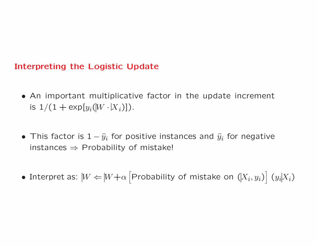
Interpreting the Logistic Update

• An important multiplicative factor in the update increment

is 1/(1 + exp[yi(W ·Xi)]).

• This factor is 1− yi for positive instances and yi for negative

instances ⇒ Probability of mistake!

• Interpret as: W ⇐ W+α[Probability of mistake on (Xi, yi)

](yiXi)

Comparing Updates of Different Models

• The unregularized updates of the perceptron, SVM, Widrow-Hoff, and logistic regression can all be written in the followingform:

W ⇐ W + αyiδ(Xi, yi)Xi

• The quantity δ(Xi, yi) is a mistake function, which is:

– Raw mistake value (1− yi(W ·Xi)) for Widrow-Hoff

– Mistake indicator whether (0− yi(W ·Xi)) > 0 for percep-tron.

– Margin/mistake indicator whether (1− yi(W ·Xi)) > 0 forSVM.

– Probability of mistake on (Xi, yi) for logistic regression.

Comparing Loss Functions of Different Models

−3 −2 −1 0 1 2 3−1

−0.5

0

0.5

1

1.5

2

2.5

3

3.5

4

PREDICTION= W.X FOR X IN POSITIVE CLASS

PE

NA

LTY

PERCEPTRON (SURROGATE)

WIDROW−HOFF/FISHER

SVM HINGE

LOGISTIC

DECISIONBOUNDARY

INCORRECTPREDICTIONS

CORRECTPREDICTIONS

• Loss functions are similar (note Widrow-Hoff retrogression).

Other Comments on Logistic Regression

• Many classical neural models use repeated computational

units with logistic and tanh activation functions in hidden

layers.

• One can view these methods as feature engineering models

that stack multiple logistic regression models.

• The stacking of multiple models creates inherently more pow-

erful models than their individual components.

Charu C. Aggarwal



The Softmax Activation Function and

Multinomial Logistic Regression



Binary Classes versus Multiple Classes

• All the models discussed so far discuss only the binary class

setting in which the class label is drawn from {−1,+1}.

• Many natural applications contain multiple classes without a

natural ordering among them:

– Predicting the category of an image (e.g., truck, carrot).

– Language models: Predict the next word in a sentence.

• Models like logistic regression are naturally designed to pre-

dict two classes.

Generalizing Logistic Regression

• Logistic regression produces probabilities of the two out-comes of a binary class.

• Multinomial logistic regression produces probabilities of mul-tiple outcomes.

– In order to produce probabilities of multiple classes, weneed an activation function with a vector output of prob-abilities.

– The softmax activation function is a vector-based gener-alization of the sigmoid activation used in logistic regres-sion.

• Multinomial logistic regression is also referred to as softmaxclassifier.

The Softmax Activation Function

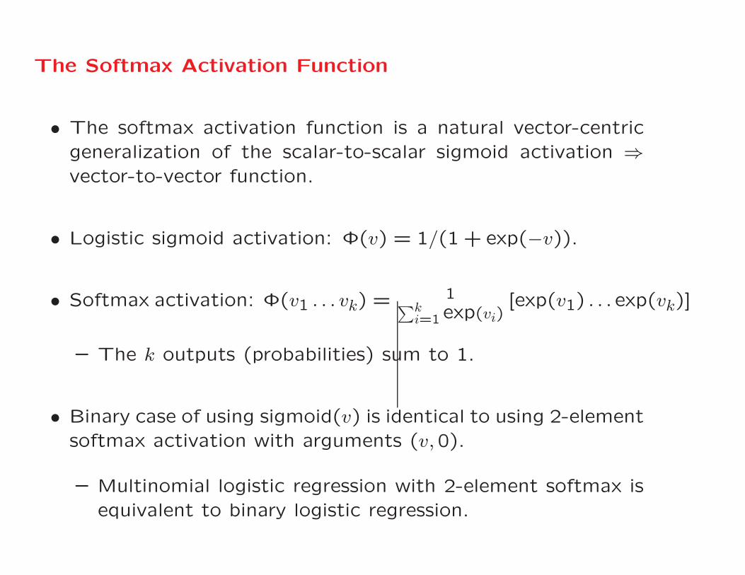
• The softmax activation function is a natural vector-centricgeneralization of the scalar-to-scalar sigmoid activation ⇒vector-to-vector function.

• Logistic sigmoid activation: Φ(v) = 1/(1 + exp(−v)).

• Softmax activation: Φ(v1 . . . vk) = 1∑ki=1exp(vi)

[exp(v1) . . . exp(vk)]

– The k outputs (probabilities) sum to 1.

• Binary case of using sigmoid(v) is identical to using 2-elementsoftmax activation with arguments (v,0).

– Multinomial logistic regression with 2-element softmax isequivalent to binary logistic regression.

Loss Functions for Softmax

• Recall that we use the negative logarithm of the probability

of observed class in binary logistic regression.

– Natural generalization to multiple classes.

– Cross-entropy loss: Negative logarithm of the probability

of correct class.

– Probability distribution among incorrect classes has no ef-

fect.

• Softmax activation is used almost exclusively in output layer

and (almost) always paired with cross-entropy loss.

Cross-Entropy Loss of Softmax

• Like the binary logistic case, the loss L is a negative log

probability.

Softmax Probability Vector ⇒ [y1, y2, . . . yk]

[y1 . . . yk] =1∑k

i=1 exp(vi)[exp(v1) . . . exp(vk)]

• The loss is −log(yc), where c ∈ {1 . . . k} is the correct class

of that training instance.

• Cross entropy loss is −vc) + log[∑k

j=1 exp(vj)]

Loss Derivative of Softmax

• Since softmax is almost always paired with cross-entropy loss

L, we can directly estimate ∂L∂vr

for each pre-activation value

from v1 . . . vk.

• Differentiate loss value of −vc + log[∑k

j=1 exp(vj)]

• Like the sigmoid derivative, the result is best expressed in

terms of the post-activation values y1 . . . yk.

• The loss derivative of the softmax is as follows:

∂L

∂vr=

⎧⎨⎩yr − 1 If r is correct class

yr If r is not correct class

Multinomial Logistic Regression

LOSS = -LOG(- ŷ2)

X

vi =

v1

∑

∑

∑

v2

v3 W3

W2

W1

Wi X

TRUE CLASS

ŷ2 = exp(v2)/[∑exp(vi)]



SOFTMAX LAYER

• The ith training instance is (Xi, c(i)), where c(i) ∈ {1 . . . k}is class index ⇒ Learn k parameter vectors W1 . . .Wk.

– Define real-valued score vr = Wr ·Xi for rth class.

– Convert scores to probabilities y1 . . . yk with softmax acti-vation on v1 . . . vk ⇒ Hard or soft prediction

Computing the Derivative of the Loss

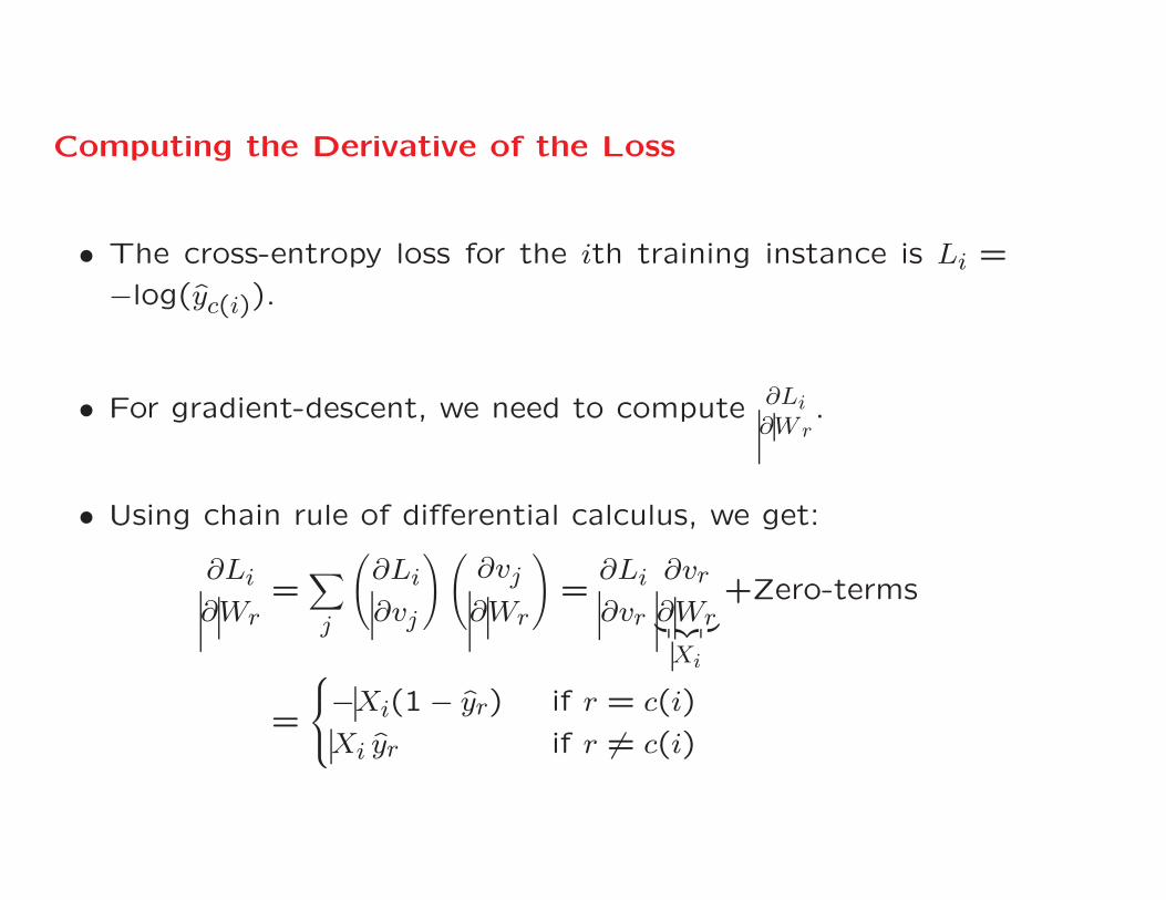
• The cross-entropy loss for the ith training instance is Li =

−log(yc(i)).

• For gradient-descent, we need to compute ∂Li∂Wr

.

• Using chain rule of differential calculus, we get:

∂Li

∂Wr=∑j

(∂Li

∂vj

)(∂vj

∂Wr

)=

∂Li

∂vr

∂vr

∂Wr︸︷︷︸Xi

+Zero-terms

=

⎧⎨⎩−Xi(1− yr) if r = c(i)

Xi yr if r �= c(i)

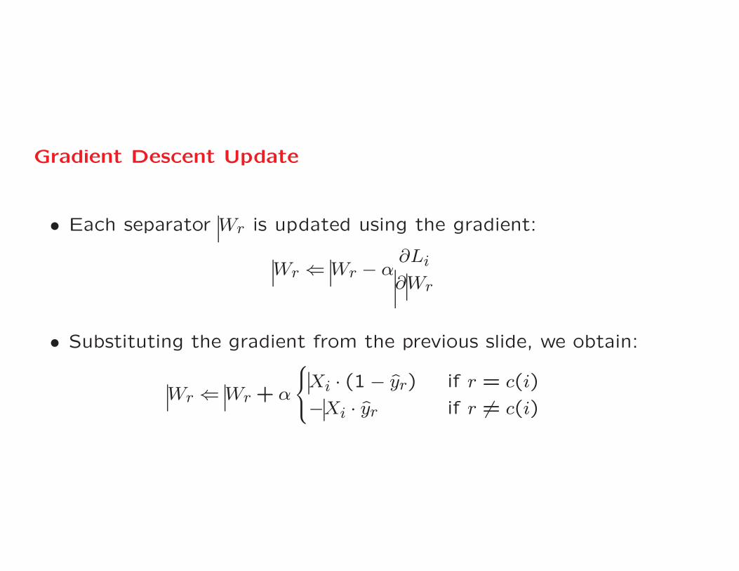
Gradient Descent Update

• Each separator Wr is updated using the gradient:

Wr ⇐ Wr − α∂Li

∂Wr

• Substituting the gradient from the previous slide, we obtain:

Wr ⇐ Wr + α

⎧⎨⎩Xi · (1− yr) if r = c(i)

−Xi · yr if r �= c(i)

Summary

• The book also contains details of the multiclass Perceptronand Weston-Watkins SVM.

• Multinomial logistic regression is a direct generalization oflogistic regression.

• If we apply the softmax classifier with two classes, we willobtain W1 = −W2 to be the same separator as obtained inlogistic regression.

• Cross-entropy loss and softmax are almost always paired inoutput layer (for all types of architectures).

– Many of the calculus derivations in previous slides are re-peatedly used in different settings.

Charu C. Aggarwal



The Autoencoder for Unsupervised

Representation Learning



Unsupervised Learning

• The models we have discussed so far use training pairs of

the form (X, y) in which the feature variables X and target

y are clearly separated.

– The target variable y provides the supervision for the learn-

ing process.

• What happens when we do not have a target variable?

– We want to capture a model of the training data without

the guidance of the target.

– This is an unsupervised learning problem.

Example

• Consider a 2-dimensional data set in which all points aredistributed on the circumference of an origin-centered circle.

• All points in the first and third quadrant belong to class +1and remaining points are −1.

– The class variable provides focus to the learning processof the supervised model.

– An unsupervised model needs to recognize the circularmanifold without being told up front.

– The unsupervised model can represent the data in only 1dimension (angular position).

• Best way of modeling is data-set dependent ⇒ Lack of su-pervision causes problems

Unsupervised Models and Compression

• Unsupervised models are closely related to compression be-

cause compression captures a model of regularities in the

data.

– Generative models represent the data in terms of a com-

pressed parameter set.

– Clustering models represent the data in terms of cluster

statistics.

– Matrix factorization represents data in terms of low-rank

approximations (compressed matrices).

• An autoencoder also provides a compressed representation

of the data.

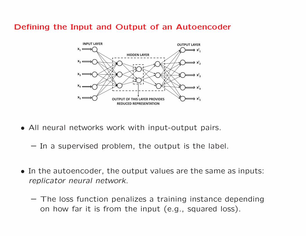
Defining the Input and Output of an Autoencoder

INPUT LAYER

HIDDEN LAYER

OUTPUT LAYER

xI4

xI3

xI2

xI1

xI5

OUTPUT OF THIS LAYER PROVIDES REDUCED REPRESENTATION

x4

x3

x2

x1

x5

• All neural networks work with input-output pairs.

– In a supervised problem, the output is the label.

• In the autoencoder, the output values are the same as inputs:replicator neural network.

– The loss function penalizes a training instance dependingon how far it is from the input (e.g., squared loss).

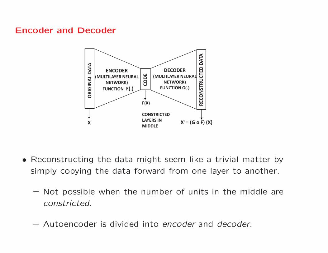
Encoder and Decoder

ORIGINAL

DATA

RECO

NSTRU

CTED

DATA

CODE

ENCODER(MULTILAYER NEURAL

NETWORK)FUNCTION F(.)

DECODER(MULTILAYER NEURAL

NETWORK)FUNCTION G(.)

X XI = (G o F) (X)

F(X)

CONSTRICTEDLAYERS INMIDDLE

• Reconstructing the data might seem like a trivial matter by

simply copying the data forward from one layer to another.

– Not possible when the number of units in the middle are

constricted.

– Autoencoder is divided into encoder and decoder.

Basic Structure of Autoencoder

• It is common (but not necessary) for an M-layer autoen-

coder to have a symmetric architecture between the input

and output.

– The number of units in the kth layer is the same as that

in the (M − k +1)th layer.

• The value of M is often odd, as a result of which the (M +

1)/2th layer is often the most constricted layer.

– We are counting the (non-computational) input layer as

the first layer.

– The minimum number of layers in an autoencoder would

be three, corresponding to the input layer, constricted

layer, and the output layer.

Undercomplete Autoencoders and Dimensionality

Reduction

• The number of units in each middle layer is typically fewer

than that in the input (or output).

– These units hold a reduced representation of the data, and

the final layer can no longer reconstruct the data exactly.

• This type of reconstruction is inherently lossy.

• The activations of hidden layers provide an alternative to

linear and nonlinear dimensionality reduction techniques.

Overcomplete Autoencoders and Representation Learning

• What happens if the number of units in hidden layer is equal

to or larger than input/output layers?

– There are infinitely many hidden representations with zero

error.

– The middle layers often do not learn the identity function.

– We can enforce specific properties on the redundant repre-

sentations by adding constraints/regularization to hidden

layer.

∗ Training with stochastic gradient descent is itself a form

of regularization.

∗ One can learn sparse features by adding sparsity con-

straints to hidden layer.

Applications

• Dimensionality reduction ⇒ Use activations of constrictedhidden layer

• Sparse feature learning ⇒ Use activations of con-strained/regularized hidden layer

• Outlier detection: Find data points with larger reconstructionerror

– Related to denoising applications

• Generative models with probabilistic hidden layers (varia-tional autoencoders)

• Representation learning ⇒ Pretraining

Charu C. Aggarwal



Singular Value Decomposition with

Autoencoders



Singular Value Decomposition

• Truncated SVD is the approximate decomposition of an n×d

matrix D into D ≈ QΣPT , where Q, Σ, and P are n×k, k×k,

and d× k matrices, respectively.

– Orthonormal columns of each of P , Q, and nonnegative

diagonal matrix Σ.

– Minimize the squared sum of residual entries in D−QΣPT .

– The value of k is typically much smaller than min{n, d}.

– Setting k to min{n, d} results in a zero-error decomposi-

tion.

Relaxed and Unnormalized Definition of SVD

• Two-way Decomposition: Find and n × k matrix U , and

d× k matrix V so that ||D − UV T ||2 is minimized.

– Property: At least one optimal pair U and V will have

mutually orthogonal columns (but non-orthogonal alter-

natives will exist).

– The orthogonal solution can be converted into the 3-way

factorization of SVD.

– Exercise: Given U and V with orthogonal columns, find

Q, Σ and P .

• In the event that U and V have non-orthogonal columns at

optimality, these columns will span the same subspace as the

orthogonal solution at optimality.

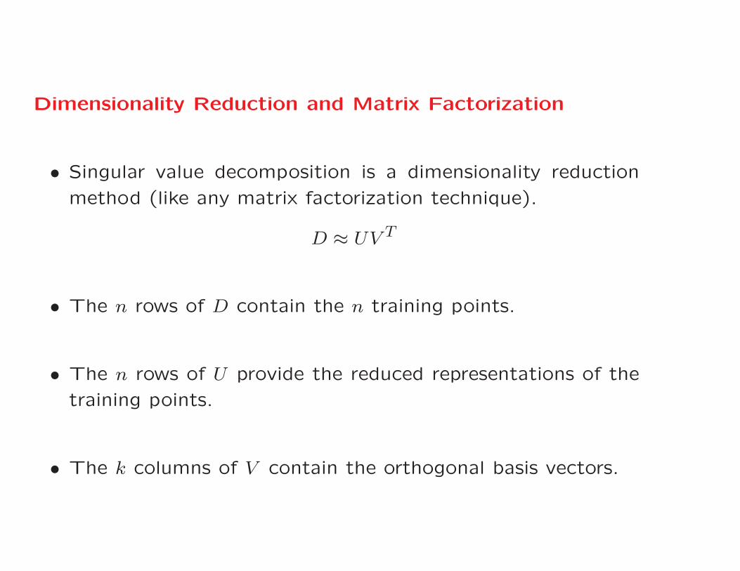
Dimensionality Reduction and Matrix Factorization

• Singular value decomposition is a dimensionality reduction

method (like any matrix factorization technique).

D ≈ UV T

• The n rows of D contain the n training points.

• The n rows of U provide the reduced representations of the

training points.

• The k columns of V contain the orthogonal basis vectors.

The Autoencoder Architecture for SVD

INPUT LAYER

OUTPUT OF THIS LAYER PROVIDES REDUCED REPRESENTATION

x4

x3

x2

x1

x5

WT

OUTPUT LAYER

xI4

xI3

xI2

xI1

xI5

VT

• The rows of the matrix D are input to encoder.

• The activations of hidden layer are rows of U and the weightsof the decoder contain V .

• The reconstructed data contain the rows of UV T .

Why is this SVD?

• If we use the mean-squared error as the loss function, we are

optimizing ||D − UV T ||2 over the entire training data.

– This is the same objective function as SVD!

• It is possible for gradient-descent to arrive at an optimal

solution in which the columns of each of U and V might not

be mutually orthogonal.

• Nevertheless, the subspace spanned by the columns of each

of U and V will always be the same as that found by the

optimal solution of SVD.

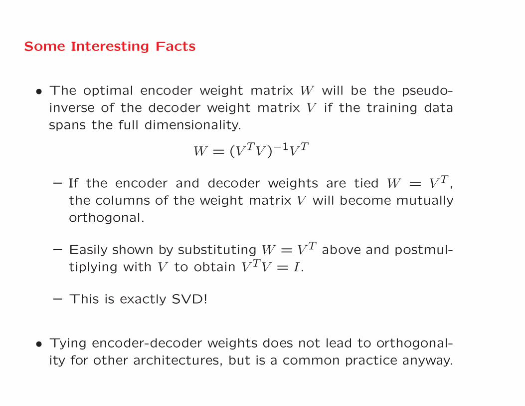
Some Interesting Facts

• The optimal encoder weight matrix W will be the pseudo-inverse of the decoder weight matrix V if the training dataspans the full dimensionality.

W = (V TV )−1V T

– If the encoder and decoder weights are tied W = V T ,the columns of the weight matrix V will become mutuallyorthogonal.

– Easily shown by substituting W = V T above and postmul-tiplying with V to obtain V TV = I.

– This is exactly SVD!

• Tying encoder-decoder weights does not lead to orthogonal-ity for other architectures, but is a common practice anyway.

Deep Autoencoders

−1

−0.5

0

0.5

1

−1

−0.5

0

0.5

1

1.5−0.2

0

0.2

0.4

0.6

0.8

1

1.2

POINT A

POINT C

POINT B

−5

0

5

−0.6−0.4

−0.20

0.20.4

0.6

−0.6

−0.4

−0.2

0

0.2

0.4

0.6

POINT A

POINT B POINT C

• Better reductions are obtained by using increased depth and

nonlinearity.

• Crucial to use nonlinear activations with deep autoencoders.

Charu C. Aggarwal



Row-Index to Row-Value Autoencoders:

Incomplete Matrix Factorization for

Recommender Systems



Recommender Systems

• Recap of SVD: Factorizes D ≈ UV T so that the sum-of-

squares of residuals ||D − UV T ||2 is minimized.

– Helpful to watch previous lecture on SVD

• In recommender systems (RS), we have an n×d ratings matrix

D with n users and d items.

– Most of the entries in the matrix are unobserved

– Want to minimize ||D − UV T ||2 only over the observed

entries

– Can reconstruct the entire ratings matrix using UV T ⇒Most popular method in traditional machine learning.

Difficulties with Autoencoder

• If some of the inputs are missing, then using an autoencoder

architecture will implicitly assume default values for some

inputs (like zero).

– This is a solution used in some recent methods like Au-

toRec.

– Does not exactly simulate classical MF used in recom-

mender systems because it implicitly makes assumptions

about unobserved entries.

• None of the proposed architectures for recommender systems

in the deep learning literature exactly map to the classical

factorization method of recommender systems.

Row-Index-to-Row-Value Autoencoder

• Autoencoders map row values to row values.

– Discuss an autoencoder architecture to map the one-hot

encoded row index to the row values.

– Not standard definition of autoencoder.

– Can handle incomplete values but cannot handle out-of-

sample data.

– Also useful for representation learning (e.g., node repre-

sentation of graph adjacency matrix).

• The row-index-to-row-value architecture is not recognized

as a separate class of architectures for MF (but used often

enough to deserve recognition as a class of MF methods).

Row-Index-to-Row-Value Autoencoder for RS

0

1

0

0

5

MISSING

4

ALICE

BOB

SAYANI

JOHN

ONE-HOT ENCODED INPUT

SHREK

E.T.

NIXON

GANDHI

NERO

MISSING

MISSING

U VT

USERS ITEMS

• Encoder and decoder weight matrices are U and V T .

– Input is one-hot encoded row index (only in-sample)

– Number of nodes in hidden layer is factorization rank.

– Outputs contain the ratings for that row index.

How to Handle Incompletely Specified Entries?

0

1

0

0

5

4 ALICE

BOB

SAYANI

JOHN

SHREK

E.T.

OBSERVED RATINGS (SAYANI): E.T., SHREK

0

0

1

0

5

ALICE

BOB

SAYANI

JOHN

E.T.

NIXON

GANDHI

NERO

4

3

2

OBSERVED RATINGS (BOB): E.T., NIXON, GANDHI, NERO

• Each user has his/her own neural architecture with missing

outputs.

• Weights across different user architectures are shared.

Equivalence to Classical Matrix Factorization for RS

• Since the two weight matrices are U and V T , the one-hot

input encoding will pull out the relevant row from UV T .

• Since the outputs only contain the observed values, we are

optimizing the sum-of-square errors over observed values.

• Objective functions in the two cases are equivalent!

Training Equivalence

• For k hidden nodes, there are k paths between each user and

each item identifier.

• Backpropagation updates weights along all k paths from each

observed item rating to the user identifier.

– Backpropagation in a later lecture.

• These k updates can be shown to be identical to classical ma-

trix factorization updates with stochastic gradient descent.

• Backpropagation on neural architecture is identical to classi-

cal MF stochastic gradient descent.

Advantage of Neural View over Classical MF View

• The neural view provides natural ways to add power to thearchitecture with nonlinearity and depth.

– Much like a child playing with a LEGO toy.

– You are shielded from the ugly details of training by aninherent modularity in neural architectures.

– The name of this magical modularity is backpropagation.

• If you have binary data, you can add logistic outputs forlogistic matrix factorization.

• Word2vec belongs to this class of architectures (but directrelationship to nonlinear matrix factorization is not recog-nized).

Importance of Row-Index-to-Row-Value Autoencoders

• Several MF methods in machine learning can be expressed

as row-index-to-row-value autoencoders (but not widely

recognized–RS matrix factorization a notable example).

• Several row-index-to-row-value architectures in NN literature

are also not fully recognized as matrix factorization methods.

– The full relationship of word2vec to matrix factorization

is often not recognized.

– Indirect relationship to linear PPMI matrix factorization

was shown by Levy and Goldberg.

– In a later lecture, we show that word2vec is directly a form

of nonlinear matrix factorization because of its row-index-

to-row-value architecture and nonlinear activation.

Charu C. Aggarwal



Word2vec: The Skipgram Model



Word2Vec: An Overview

• Word2vec computes embeddings of words using sequential

proximity in sentences.

– If Paris is closely related to France, then Paris and France

must occur together in small windows of sentences.

∗ Their embeddings should also be somewhat similar.

– Continuous bag-of-words predicts central word from con-

text window.

– Skipgram model predicts context window from central

word.

Words and Context

• A window of size t on either side is predicted using a word.

• This model tries to predict the context wi−twi−t+1 . . . wi−1

wi+1 . . . wi+t−1wi+t around word wi, given the ith word in

the sentence, denoted by wi.

• The total number of words in the context window is m = 2t.

• One can also create a d × d word-context matrix C with

frequencies cij.

• We want to find an embedding of each word.

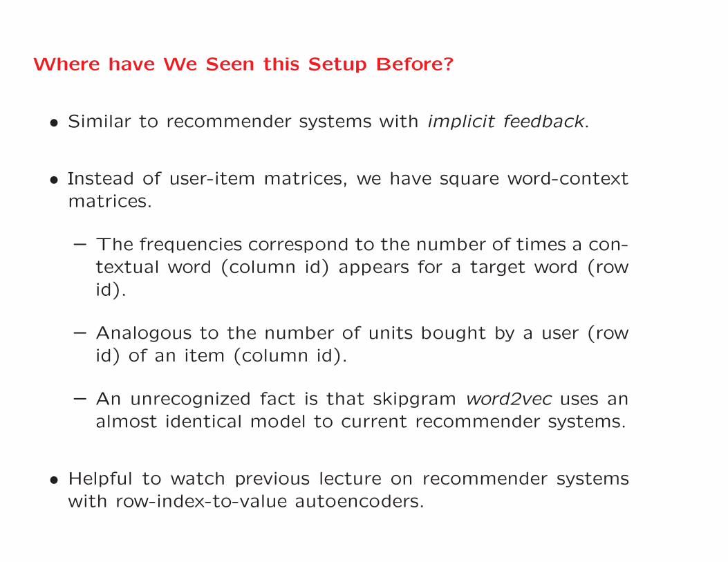
Where have We Seen this Setup Before?

• Similar to recommender systems with implicit feedback.

• Instead of user-item matrices, we have square word-contextmatrices.

– The frequencies correspond to the number of times a con-textual word (column id) appears for a target word (rowid).

– Analogous to the number of units bought by a user (rowid) of an item (column id).

– An unrecognized fact is that skipgram word2vec uses analmost identical model to current recommender systems.

• Helpful to watch previous lecture on recommender systemswith row-index-to-value autoencoders.

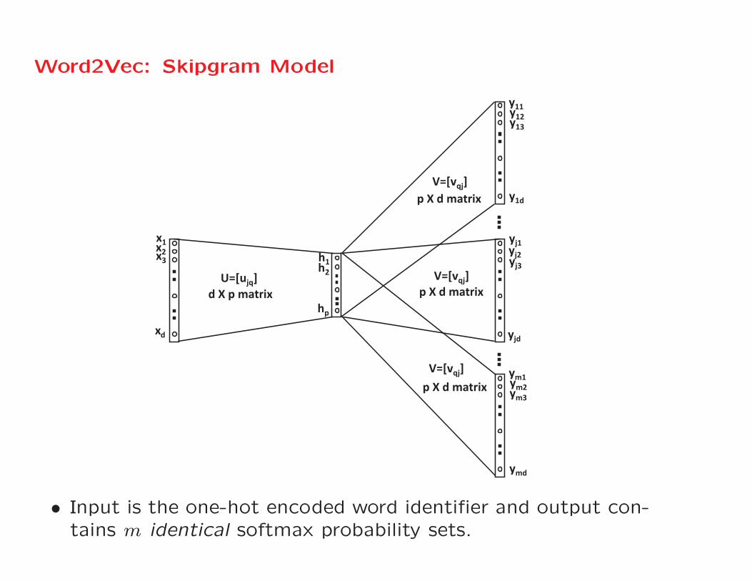
Word2Vec: Skipgram Model

x1x2x3

xd

h1h2

hp

y11y12y13

y1d

yj1yj2yj3

yjd

ym1ym2ym3

ymd

U=[ujq]

V=[vqj]

V=[vqj]

V=[vqj]

d X p matrix

p X d matrix

p X d matrix

p X d matrix

• Input is the one-hot encoded word identifier and output con-tains m identical softmax probability sets.

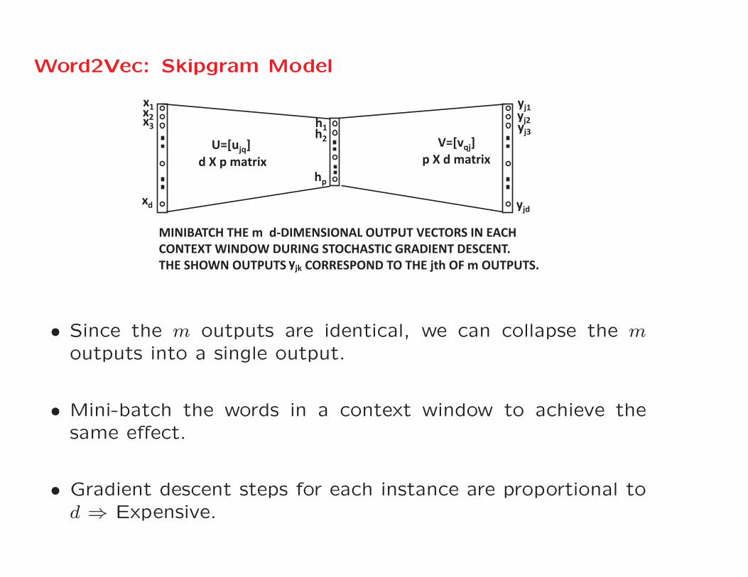
Word2Vec: Skipgram Model

x1x2x3

xd

h1h2

hp

yj1yj2yj3

yjd

U=[ujq] V=[vqj]d X p matrix p X d matrix

MINIBATCH THE m d-DIMENSIONAL OUTPUT VECTORS IN EACH CONTEXT WINDOW DURING STOCHASTIC GRADIENT DESCENT. THE SHOWN OUTPUTS CORRESPOND TO THE jth OF m OUTPUTS.yjk

• Since the m outputs are identical, we can collapse the moutputs into a single output.

• Mini-batch the words in a context window to achieve thesame effect.

• Gradient descent steps for each instance are proportional tod ⇒ Expensive.

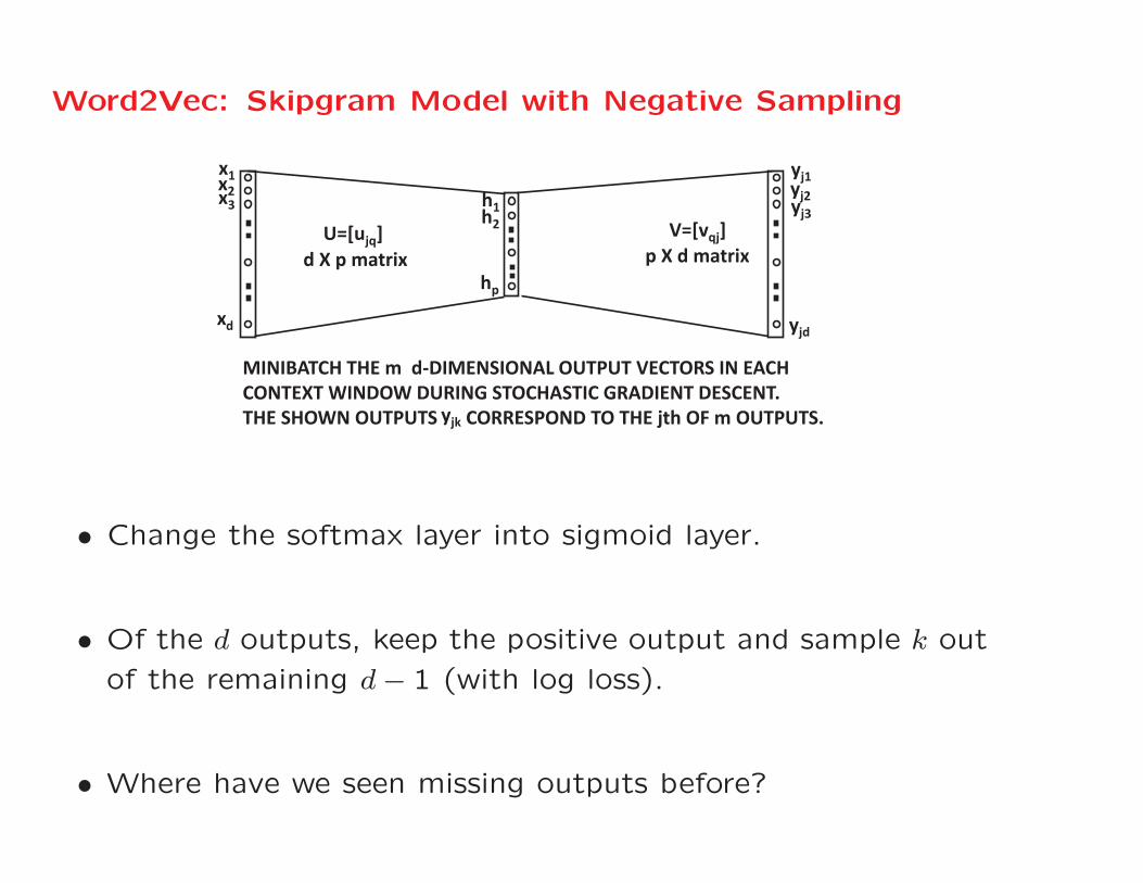
Word2Vec: Skipgram Model with Negative Sampling

x1x2x3

xd

h1h2

hp

yj1yj2yj3

yjd


MINIBATCH THE m d-DIMENSIONAL OUTPUT VECTORS IN EACH CONTEXT WINDOW DURING STOCHASTIC GRADIENT DESCENT. THE SHOWN OUTPUTS CORRESPOND TO THE jth OF m OUTPUTS.yjk

• Change the softmax layer into sigmoid layer.

• Of the d outputs, keep the positive output and sample k out

of the remaining d− 1 (with log loss).

• Where have we seen missing outputs before?

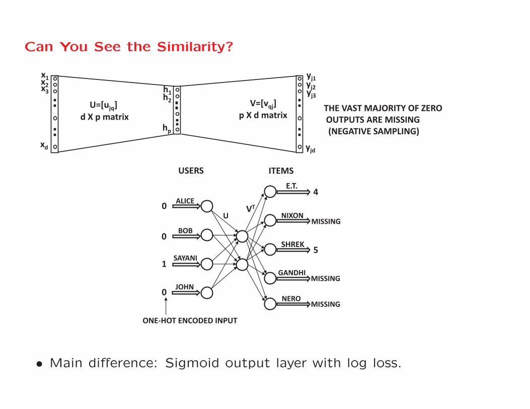
Can You See the Similarity?

x1x2x3

xd

h1h2

hp

yj1yj2yj3

yjd


THE VAST MAJORITY OF ZEROOUTPUTS ARE MISSING(NEGATIVE SAMPLING)

0

1

0

0

5

MISSING

4

ALICE

BOB

SAYANI

JOHN

ONE-HOT ENCODED INPUT

SHREK

E.T.

NIXON

GANDHI

NERO

MISSING

MISSING

U VT

USERS ITEMS

• Main difference: Sigmoid output layer with log loss.

Word2Vec is Nonlinear Matrix Factorization

• Levy and Goldberg showed an indirect relationship between

word2vec SGNS and PPMI matrix factorization.

• We provide a much more direct result in the book.

– Word2vec is (weighted) logistic matrix factorization.

– Not surprising because of the similarity with the recom-

mender architecture.

– Logistic matrix factorization is already used in recom-

mender systems!

– Neither the word2vec authors nor the community have

pointed out this direct connection.

Other Extensions

• We can apply a row-index-to-value autoencoder to any type

of matrix to learn embeddings of either rows or columns.

• Applying to graph adjacency matrix leads to node embed-

dings.

– Idea has been used by DeepWalk and node2vec after (in-

directly) enhancing the matrix entries with random-walk

methods.

– Details of graph embedding methods in book.

connecting machine learning with shallow neural networks · 2018-05-19 · the deep learning...

Documents