Consensus New KeynesianConsensus New Keynesian DSGE Model

Lawrence Christiano

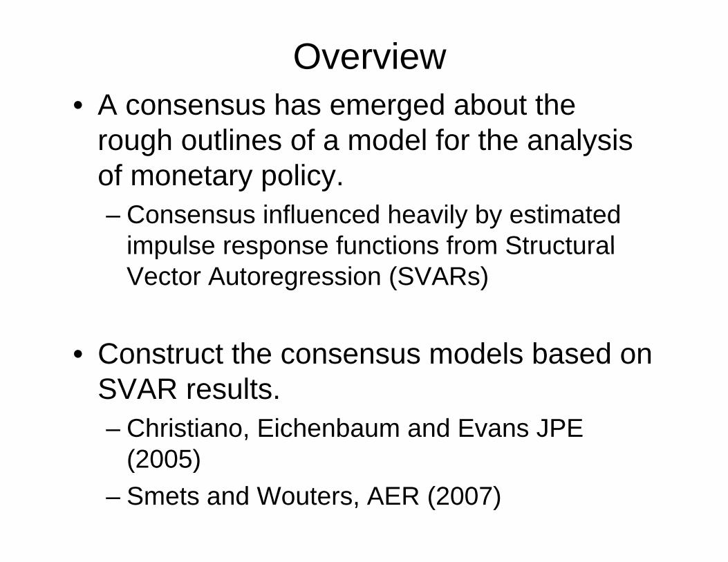
Overview• A consensus has emerged about the• A consensus has emerged about the

rough outlines of a model for the analysis of monetary policyof monetary policy.– Consensus influenced heavily by estimated

impulse response functions from Structuralimpulse response functions from Structural Vector Autoregression (SVARs)

• Construct the consensus models based on SVAR resultsSVAR results.– Christiano, Eichenbaum and Evans JPE

(2005)(2005)– Smets and Wouters, AER (2007)

• Very brief review of SVARs.

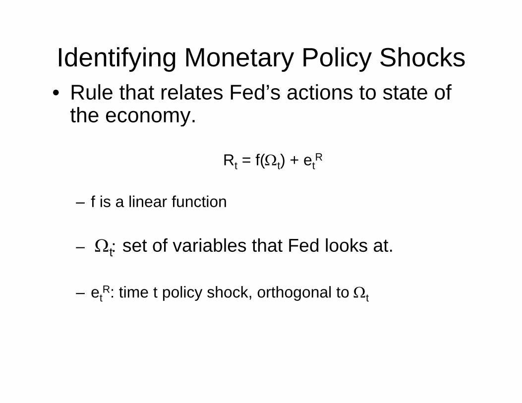
Identifying Monetary Policy Shocks• Rule that relates Fed’s actions to state of

the economy.y

Rt = f(Ωt) + etR

– f is a linear function

– Ωt: set of variables that Fed looks at.

– etR: time t policy shock, orthogonal to Ωt

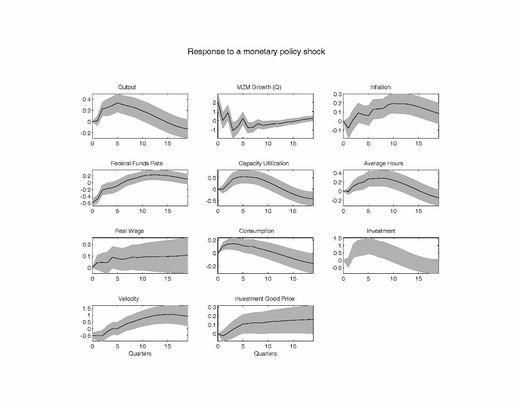
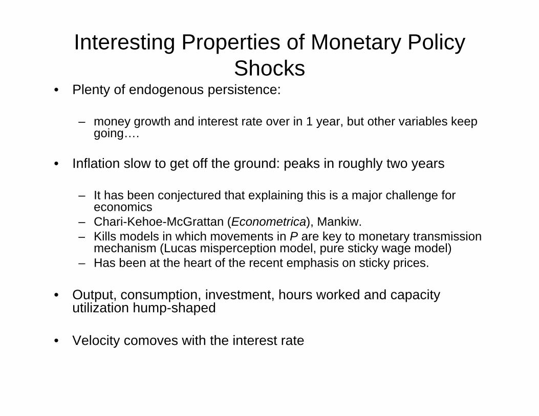
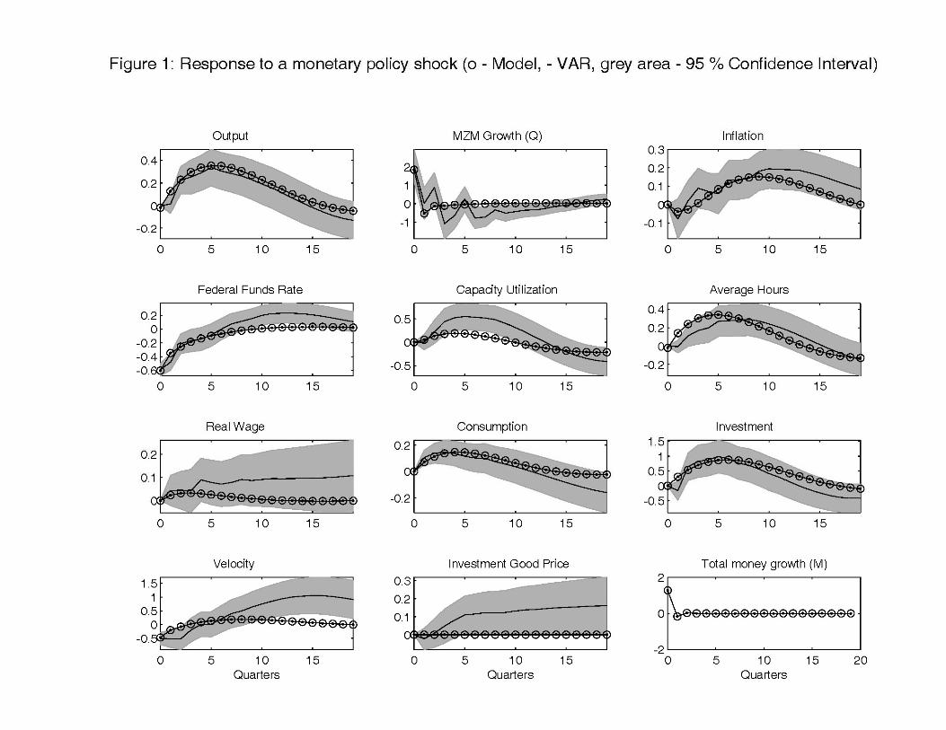
Interesting Properties of Monetary Policy Shocks

• Plenty of endogenous persistence:

– money growth and interest rate over in 1 year, but other variables keep igoing….

• Inflation slow to get off the ground: peaks in roughly two years

– It has been conjectured that explaining this is a major challenge for economics

– Chari-Kehoe-McGrattan (Econometrica), Mankiw.Kills models in which movements in P are key to monetary transmission– Kills models in which movements in P are key to monetary transmission mechanism (Lucas misperception model, pure sticky wage model)

– Has been at the heart of the recent emphasis on sticky prices.

• Output, consumption, investment, hours worked and capacity utilization hump-shaped

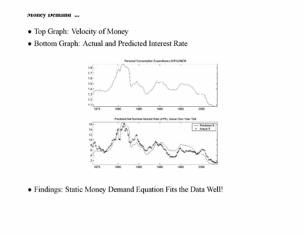
• Velocity comoves with the interest rate• Velocity comoves with the interest rate

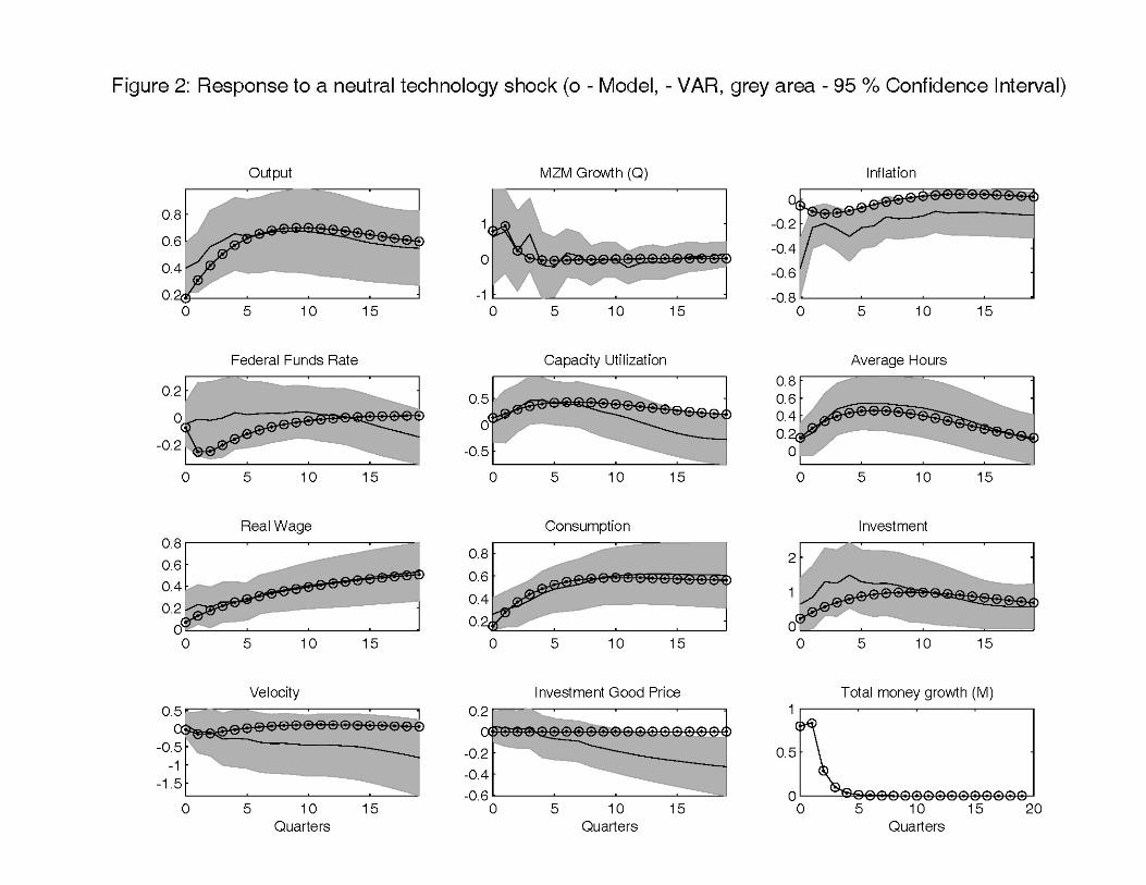
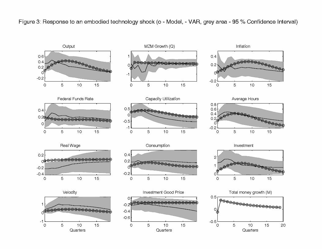
Identification of Technology ShocksShocks

• Two technology shocks:• Two technology shocks:– One perturbs price of investment goods– One perturbs total factor productivityp p y

• Identification assumptions:p– They are the only two shocks that affect labor

productivity in the long run

– Only the shock to investment good prices have an impact on investment good prices in the longan impact on investment good prices in the long run.

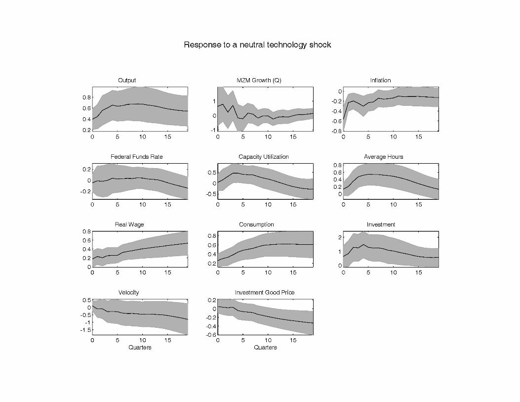
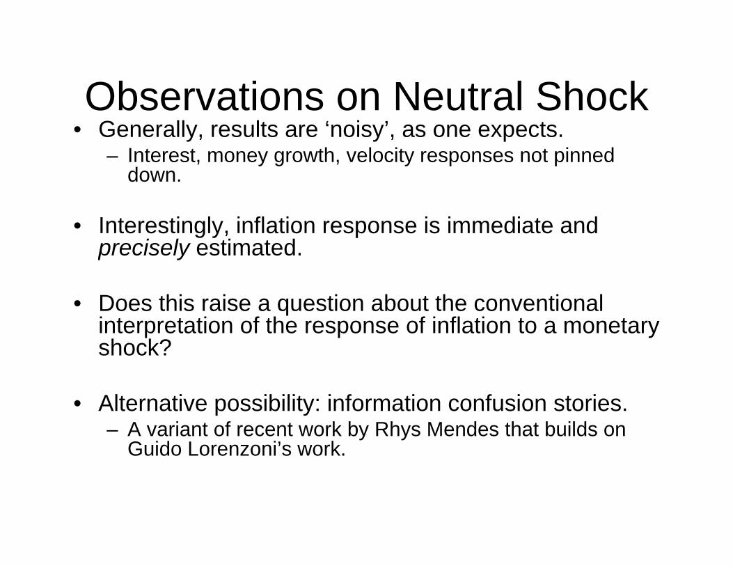
Observations on Neutral ShockObservations on Neutral Shock• Generally, results are ‘noisy’, as one expects.

– Interest, money growth, velocity responses not pinned downdown.

• Interestingly, inflation response is immediate and precisely estimatedprecisely estimated.

• Does this raise a question about the conventional i t t ti f th f i fl ti t tinterpretation of the response of inflation to a monetary shock?

• Alternative possibility: information confusion stories.– A variant of recent work by Rhys Mendes that builds on

Guido Lorenzoni’s work.

Importance of Three ShocksImportance of Three Shocks

A di t VAR l i th t• According to VAR analysis, they account for a large part of economic fluctuations.

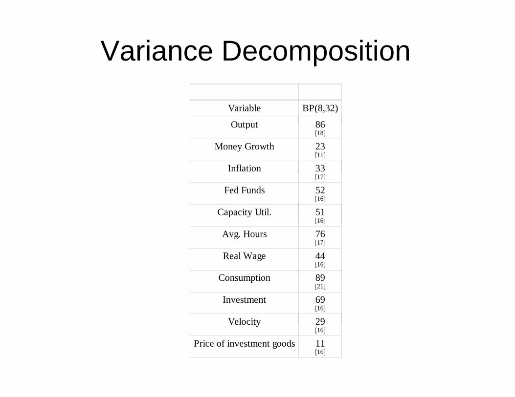
Variance Decomposition

Variable BP(8,32)

Output 86Output1886

Money Growth1123

Inflation 3317

Fed Funds1652

Capacity Util.1651

Avg. Hours1776

Real Wage1644

Consumption2189

Investment1669

Velocity 29Velocity1629

Price of investment goods1611

NextU I l R t E ti t DSGE M d l• Use Impulse Responses to Estimate a DSGE Model

– Motivate the Basic Model Features. Model Estimation– Model Estimation.

• Determine if there is a conflict regarding price behavior between micro and macro data.between micro and macro data.

– Macro Evidence:• Inflation responds slowly to monetary shock

Si l ti ti t f l f Philli d ll• Single equation estimates of slope of Phillips curve produce small slope coefficients.

– Micro Evidence:Bil Kl N k St i t id f f• Bils-Klenow, Nakamura-Steinsson report evidence on frequency of price change at micro level: 5-11 months.

• Finding: no micro macro puzzle, as long as we th t it l d b fi i ‘fi ifi ’suppose that capital used by firms is ‘firm-specific’.

Outline• Model

• Econometric Estimation of Model• Econometric Estimation of Model– Fitting Model to Impulse Response Functions

• Model Estimation Results (is there a micro/macro puzzle?)

Description of ModelDescription of Model• Timing Assumptionsg p

• Firms

• Households

• Monetary Authority

• Goods Market Clearing and Equilibrium

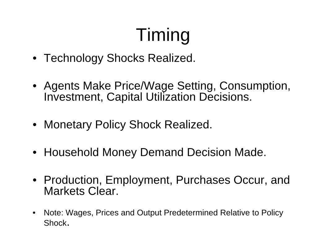
Timing• Technology Shocks Realized.

• Agents Make Price/Wage Setting, Consumption, Investment, Capital Utilization Decisions.

• Monetary Policy Shock Realized.

• Household Money Demand Decision Made.

• Production, Employment, Purchases Occur, and Markets Clear.

• Note: Wages, Prices and Output Predetermined Relative to Policy Shock.

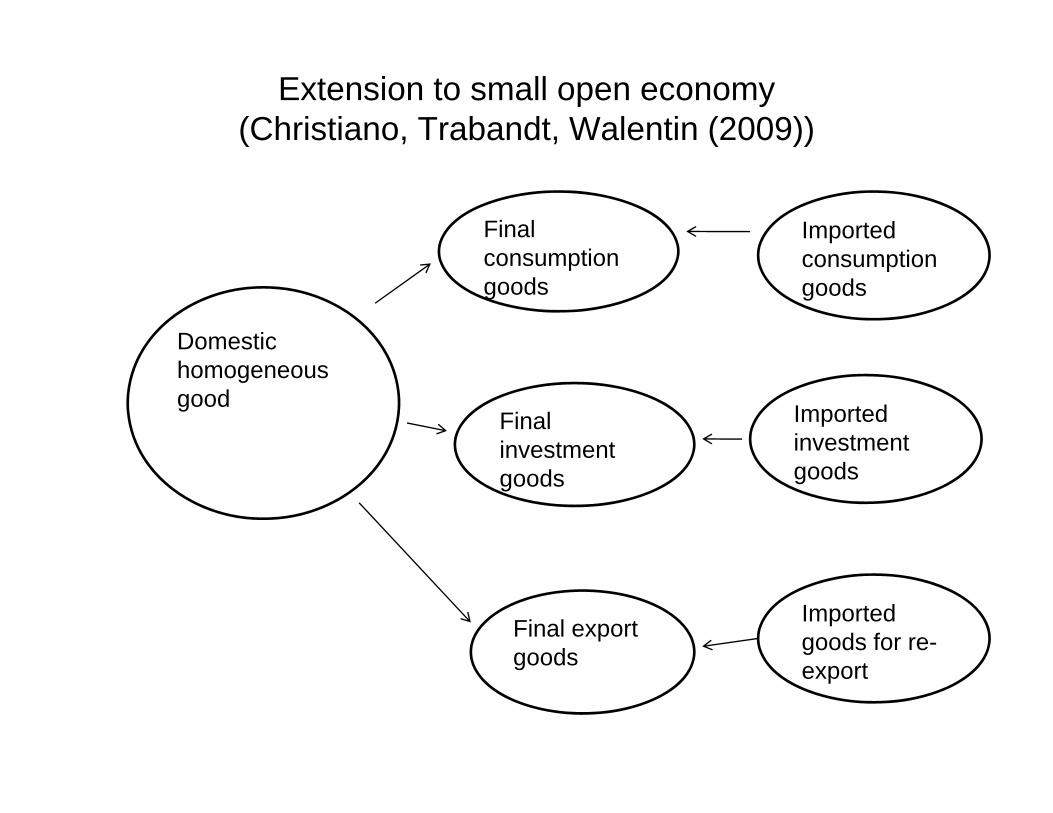
Extension to small open economy(Christiano, Trabandt, Walentin (2009))

Final ti

Imported ti

Domestic

consumption goods

consumption goods

homogeneous good

Final investment

Imported investment es e

goods goods

Final export goods

Imported goods for re-

tgoods export

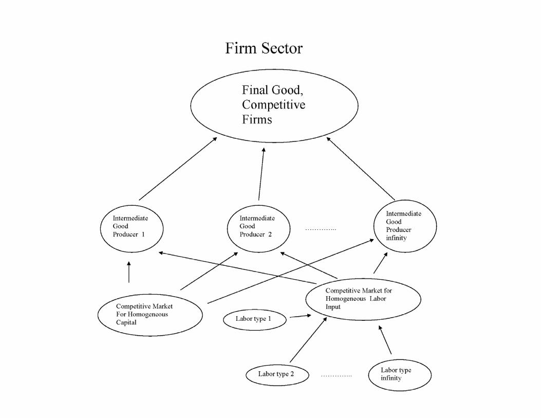
Firms• Final good firms

Technology:– Technology:

Yt 0

1 yit

1 f di

f

, 1 ≤ f

– Objective:

0yit f

1maxYt,yit,0≤i≤1 PtYt − 01 Pityitdi

– Foncs and prices:

Pt

f 1 yit P 1 P

11− f

1− fPtPit

f−1 yitYt

, Pt 0Pit

f

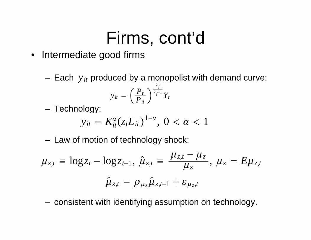
Firms, cont’d,• Intermediate good firms

E h d d b li t ith d d– Each produced by a monopolist with demand curve:yit

yit PtPit

f f−1 Yt

– Technology:yit Kit

ztLit1−, 0 1– Law of motion of technology shock:

z,t ≡ logzt − logzt−1, z,t ≡z,t − z , z Ez,t , g g t , , z

, ,

z,t zz,t−1 z,t

– consistent with identifying assumption on technology.

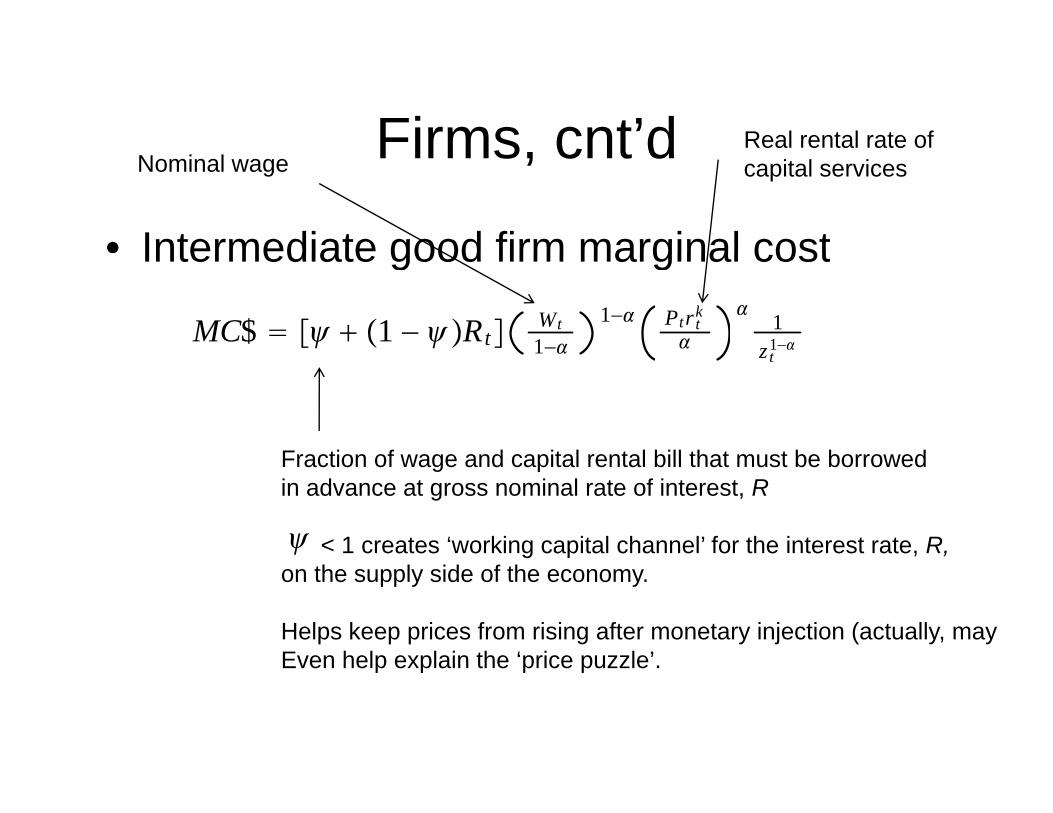
Firms cnt’d Real rental rate ofFirms, cnt d

• Intermediate good firm marginal cost

Nominal wage capital services

Intermediate good firm marginal cost

MC$ 1 − Rt Wt1−

1− Ptrtk

1

zt1−

Fraction of wage and capital rental bill that must be borrowed

zt

Fraction of wage and capital rental bill that must be borrowedin advance at gross nominal rate of interest, R

< 1 creates ‘working capital channel’ for the interest rate, R,on the supply side of the economy.

Helps keep prices from rising after monetary injection (actually, mayEven help explain the ‘price puzzle’Even help explain the price puzzle .

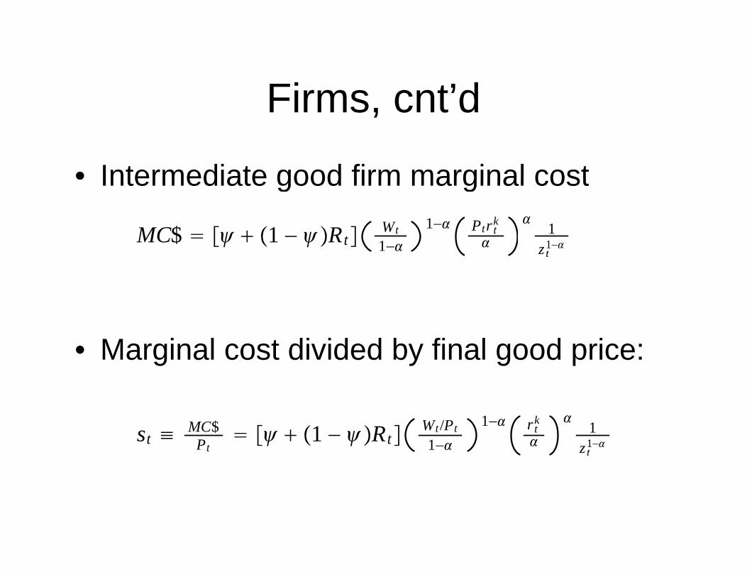
Firms cnt’dFirms, cnt d

• Intermediate good firm marginal costIntermediate good firm marginal cost

MC$ 1 − Rt Wt1−

1− Ptrtk

1

zt1−zt

• Marginal cost divided by final good price:

st ≡ MC$Pt

1 − Rt Wt/Pt1−

1− rtk

1

zt1−

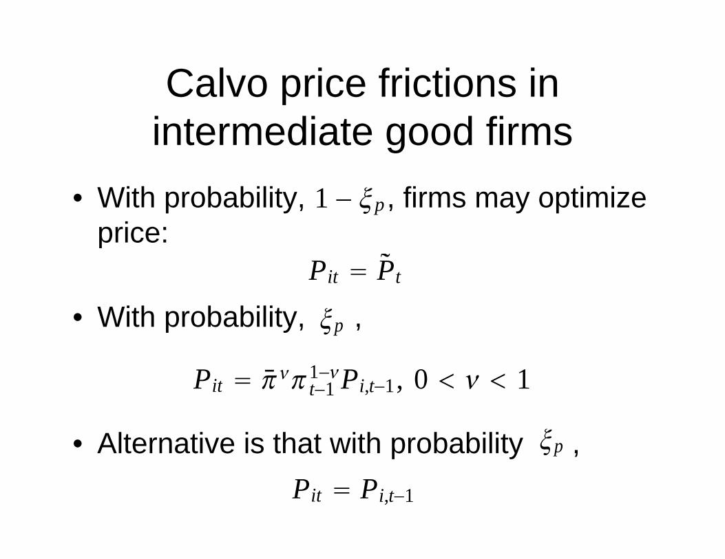
Calvo price frictions in pintermediate good firms

• With probability, , firms may optimize price:

1 − pp

• With probabilityPit Pt

• With probability, , p

Pit t 11−Pi t 1 0 1

• Alternative is that with probability ,

Pit t−1 Pi,t−1, 0 1

pp y ,p

Pit Pi,t−1

Evidence from Midrigan, ‘Menu Costs, Multi-Product Firms, and Aggregate Fluctuations’

Lot’s ofsmallchanges

Hi t f l (P /P ) diti l i dj t t f t d t tHistograms of log(Pt/Pt-1), conditional on price adjustment, for two data setspooled across all goods/stores/months in sample.

0

1 1

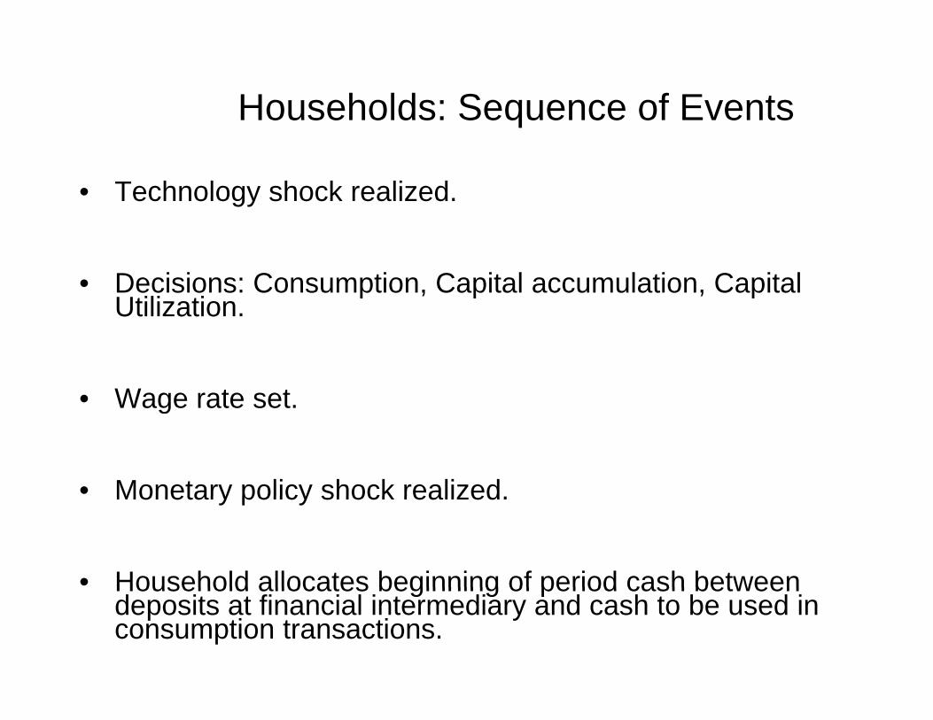
Households: Sequence of Events

• Technology shock realized.

• Decisions: Consumption, Capital accumulation, Capital Utilization.Utilization.

• Wage rate set.Wage rate set.

• Monetary policy shock realizedMonetary policy shock realized.

• Household allocates beginning of period cash betweenHousehold allocates beginning of period cash between deposits at financial intermediary and cash to be used in consumption transactions.

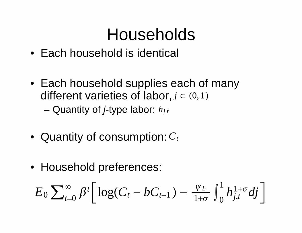
Households• Each household is identical

• Each household supplies each of many different varieties of labor, j ∈ 0,1– Quantity of j-type labor: hj,t

• Quantity of consumption: Ct

• Household preferences:

E ∑ t l C bC L 1 h1djE0∑t0 t logCt − bCt−1 −

L1 0 hj,t

1dj

Household and Labor MarketErceg Henderson Levin ModelErceg-Henderson-Levin Model

• Each type of labor, j, in the household joins a yp , j, junion of all j-type labor from all other households.

• The union for j-type labor behaves as a monopolist on behalf of its members, settingmonopolist on behalf of its members, setting the wage subject to a demand curve for j-type labor.

Wj,t

• With probability the union may not reoptimize the wage and with probability

w

1 − reoptimize the wage, and with probability it may reoptimize.

1 w

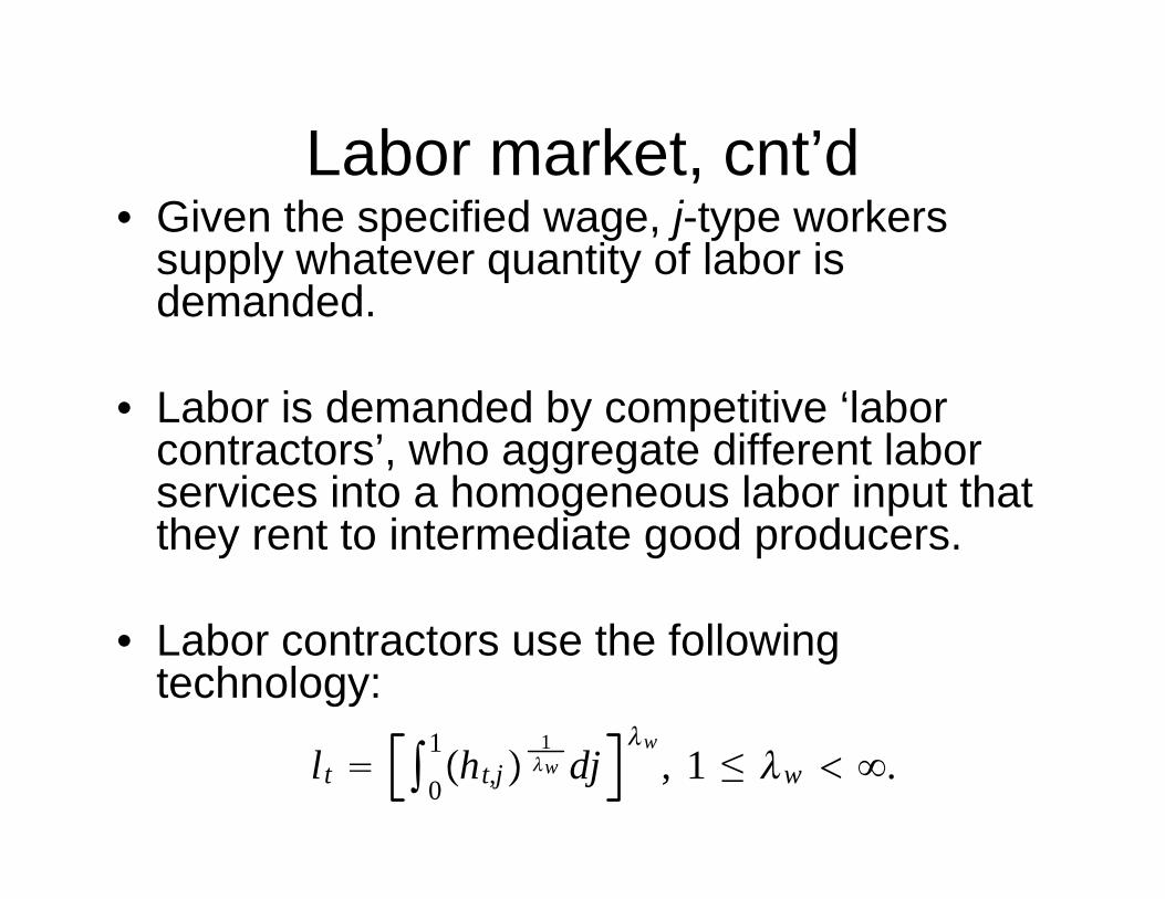
Labor market cnt’dLabor market, cnt d• Given the specified wage, j-type workers

supply whatever quantity of labor is pp y q ydemanded.

L b i d d d b titi ‘l b• Labor is demanded by competitive ‘labor contractors’, who aggregate different labor services into a homogeneous labor input thatservices into a homogeneous labor input that they rent to intermediate good producers.

• Labor contractors use the following technology:

1 lt

0

1ht,j

1w dj

w, 1 ≤ w .

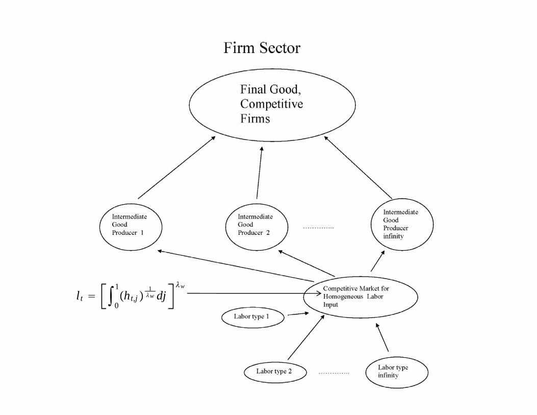
1 w

lt 0

1ht,j

1w dj

w

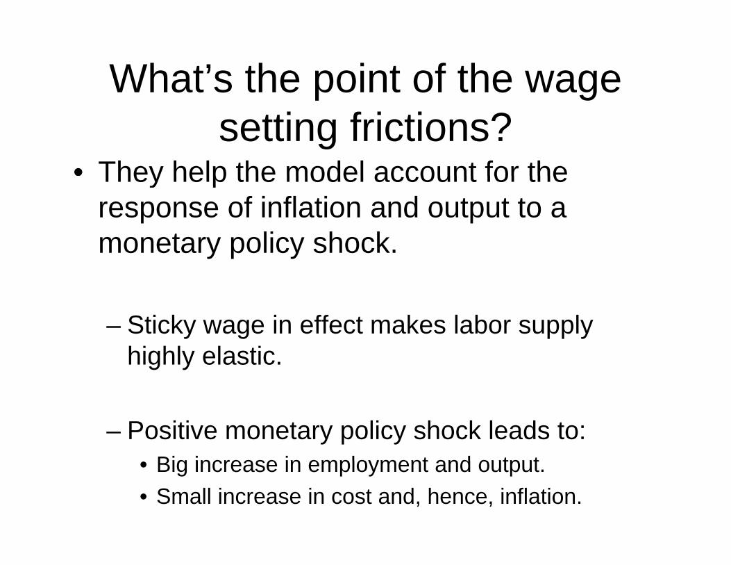
What’s the point of the wage setting frictions?

• They help the model account for theThey help the model account for the response of inflation and output to a monetary policy shockmonetary policy shock.

Sti k i ff t k l b l– Sticky wage in effect makes labor supply highly elastic.

– Positive monetary policy shock leads to:Big increase in employment and output• Big increase in employment and output.

• Small increase in cost and, hence, inflation.

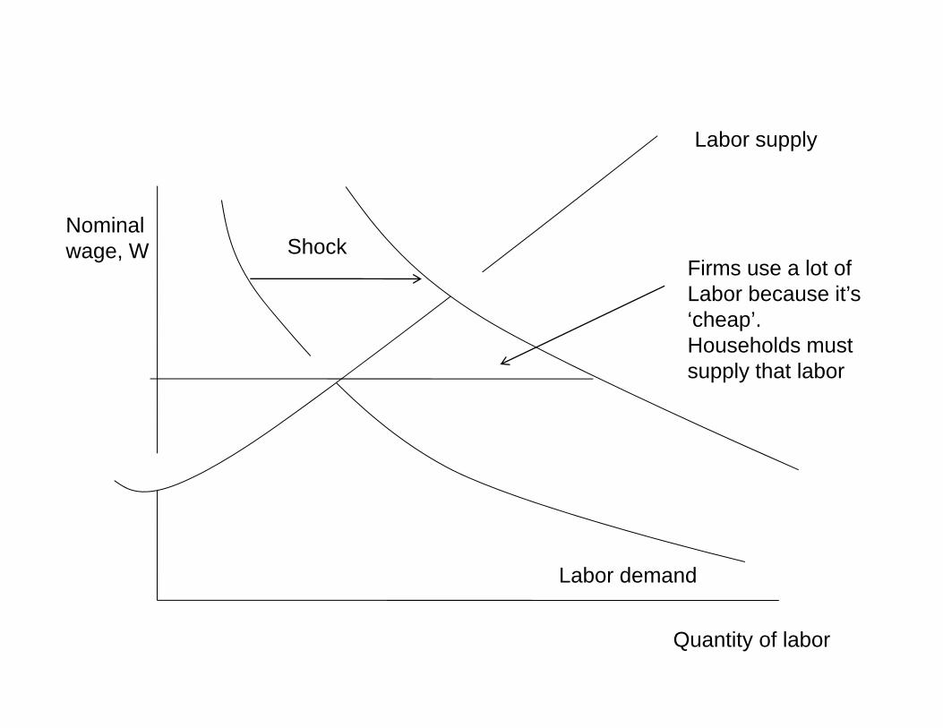
L b l

Nominal

Labor supply

Nominalwage, W Shock

Firms use a lot of Labor because it’s ‘cheap’cheap . Households mustsupply that labor

Labor demand

Quantity of labor

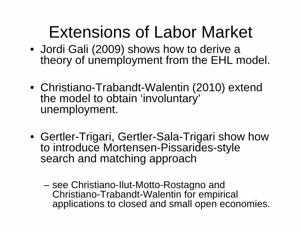
Extensions of Labor Market• Jordi Gali (2009) shows how to derive a

theory of unemployment from the EHL model.

• Christiano-Trabandt-Walentin (2010) extend the model to obtain ‘involuntary’the model to obtain involuntary unemployment.

• Gertler-Trigari, Gertler-Sala-Trigari show how to introduce Mortensen-Pissarides-style search and matching approachsearch and matching approach

– see Christiano-Ilut-Motto-Rostagno and gChristiano-Trabandt-Walentin for empirical applications to closed and small open economies.

Why Habit Persistence in Preferences?

• They help resolve the ‘consumption• They help resolve the consumption puzzle’ in monetary economics…..

• With standard preferences, hard to understand the way consumption responds to monetary policy shock.

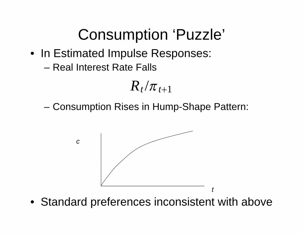
Consumption ‘Puzzle’• In Estimated Impulse Responses:

– Real Interest Rate Falls

Rt /t1

– Consumption Rises in Hump-Shape Pattern:

c

t

• Standard preferences inconsistent with abovet

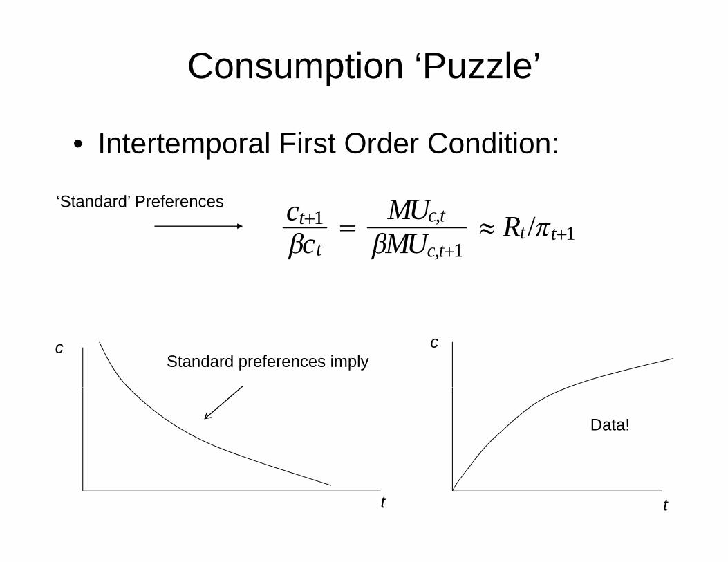
Consumption ‘Puzzle’

• Intertemporal First Order Condition:

ct1ct

MUc,tMU 1

≈ Rt/t1

‘Standard’ Preferences

ct MUc,t1

c cStandard preferences imply

Data!

t t

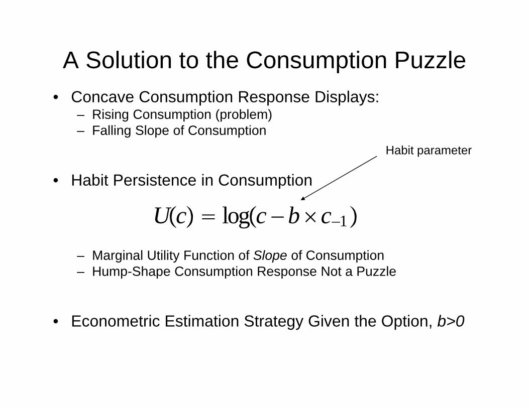
A Solution to the Consumption Puzzle• Concave Consumption Response Displays:

– Rising Consumption (problem)F lli Sl f C ti– Falling Slope of Consumption

• Habit Persistence in Consumption

Habit parameter

• Habit Persistence in Consumption

Uc logc − b c−1– Marginal Utility Function of Slope of Consumption– Hump-Shape Consumption Response Not a Puzzle

• Econometric Estimation Strategy Given the Option, b>0

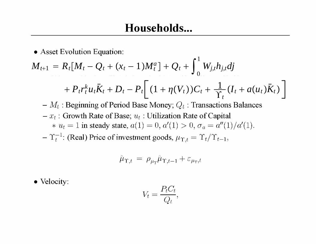
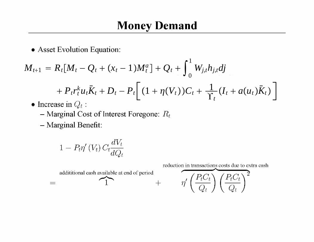
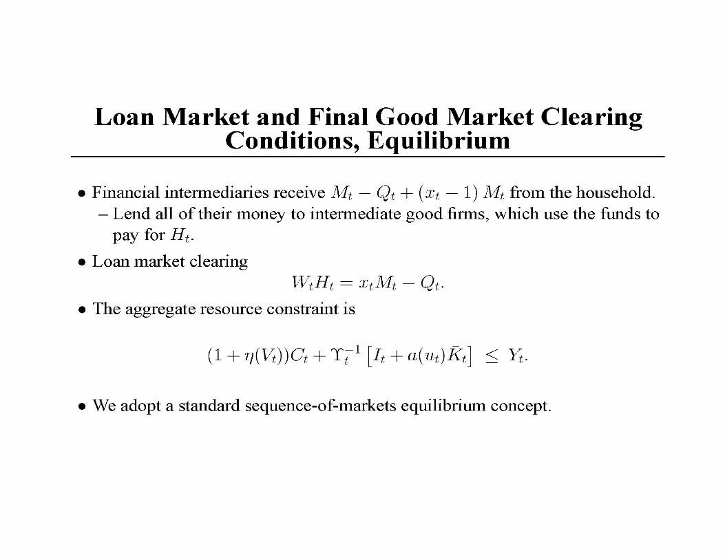
Mt1 RtMt − Qt xt − 1Mta Qt

0

1Wj,thj,tdj

0

PtrtkutKt Dt − Pt 1 VtCt 1

tIt autKt

Mt1 RtMt − Qt xt − 1Mta Qt

0

1Wj,thj,tdj

0

PtrtkutKt Dt − Pt 1 VtCt 1

tIt autKt

Dynamic Response of Investment to Monetary Policy Shock

• In Estimated Impulse Responses:

– Investment Rises in Hump-Shaped Pattern:

I

t

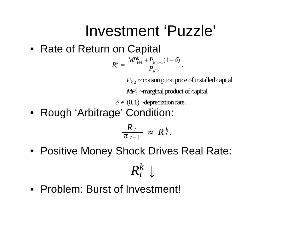
Investment ‘Puzzle’• Rate of Return on Capital

Rtk

MPt1k Pk′,t11−

Pk′,t,

k ,t

Pk′,t ~ consumption price of installed capitalMPt

k ~marginal product of capital ∈ 0 1 depreciation rate

• Rough ‘Arbitrage’ Condition: ∈ 0,1~depreciation rate.

R t R k

• Positive Money Shock Drives Real Rate:

t t1

≈ R tk .

• Problem: Burst of Investment!

Rtk ↓

• Problem: Burst of Investment!

Investment Puzzle: a failed approachAdj t t C t i I t t• Adjustment Costs in Investment– Standard Model (Lucas-Prescott)

– Problem: k′ 1− k F I

k I.

• Hump-Shape Response Creates Anticipated Capital Gains

Pk ′ t1 1I I

k ,t1Pk ′,t

1

Data!Optimal Under Standard Specification

t t

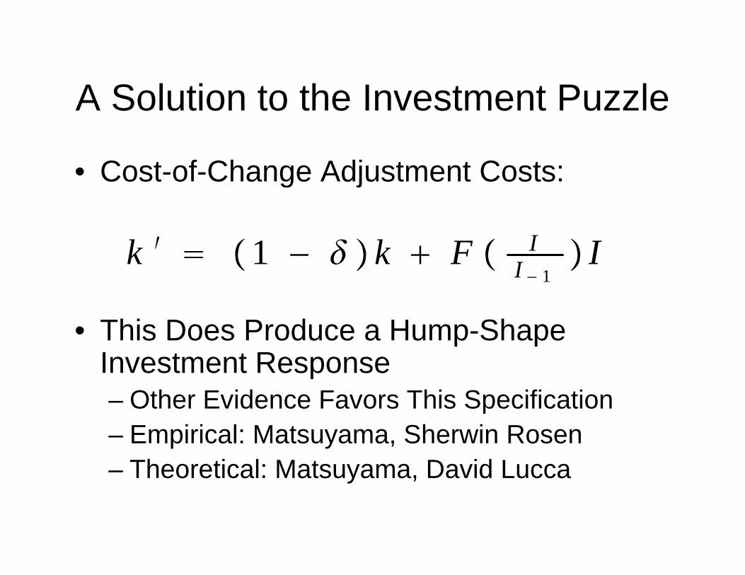
A Solution to the Investment PuzzleA Solution to the Investment Puzzle

• Cost-of-Change Adjustment Costs:Cost of Change Adjustment Costs:

k ′ 1 k F I I

Thi D P d H Sh

k 1 − k F I − 1 I

• This Does Produce a Hump-Shape Investment Response

Other Evidence Favors This Specification– Other Evidence Favors This Specification– Empirical: Matsuyama, Sherwin Rosen

Theoretical: Matsuyama David Lucca– Theoretical: Matsuyama, David Lucca

We estimate , the slope of, pthe Phillips curve, rather than

.p

1

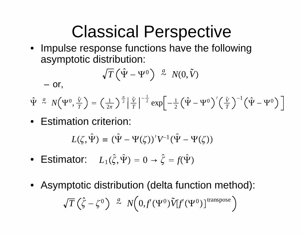
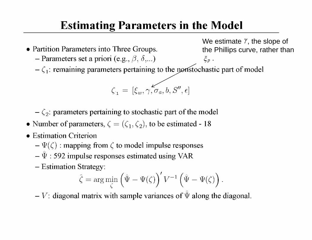
Classical Perspective• Impulse response functions have the following

asymptotic distribution:T 0 a N0 V

– or,T − 0 ~ N0,V

a N 0 V 1n2 V − 1

2 exp 1 0 ′ V −1 0

• Estimation criterion:

~ N 0, T 22

T exp − 2 − 0T − 0

• Estimator:

L, ≡ − ′V−1 −

L1 0 → fEstimator:

• Asymptotic distribution (delta function method):

L1, 0 → f

T − 0 a~ N 0, f ′0Vf ′0 transpose

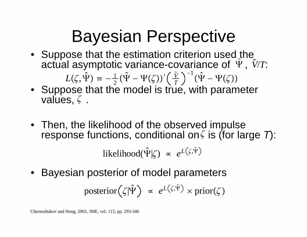
Bayesian Perspectivey p• Suppose that the estimation criterion used the

actual asymptotic variance-covariance of , : V/T 1 V −1

• Suppose that the model is true, with parameter values, .

L, ≡ − 12 −

′ VT

1 −

,

• Then, the likelihood of the observed impulse response functions conditional on is (for large T):response functions, conditional on is (for large T):

likelihood(|) eL ,

• Bayesian posterior of model parameters

posterior | eL , prior

Chernozhukov and Hong, 2003, JME, vol. 115, pp. 293-346

posterior | e prior

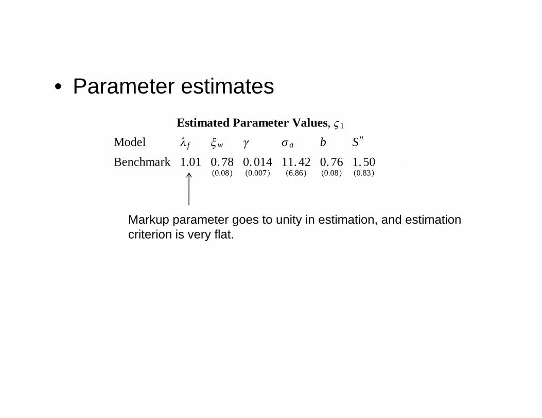
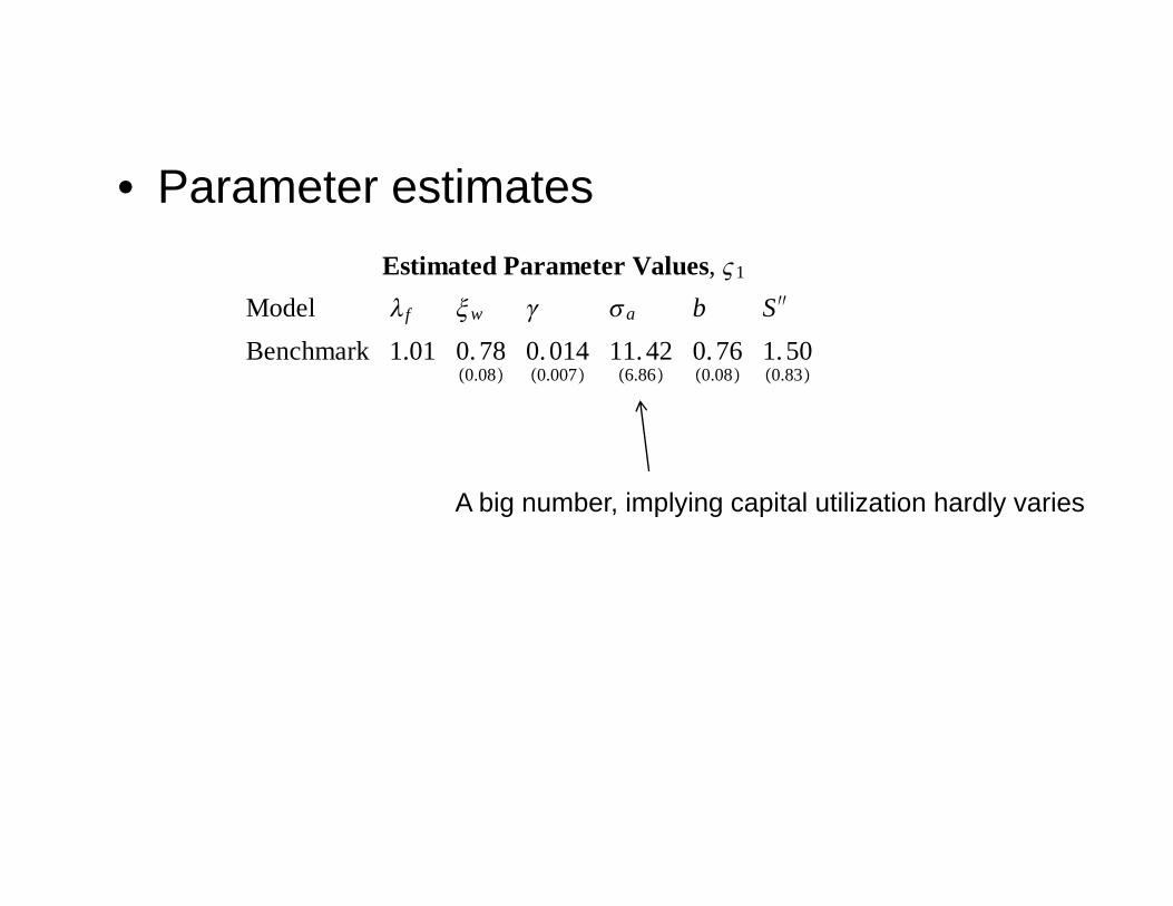
• Parameter estimatesEstimated Parameter Values, 1

Model f w a b S ′′

Benchmark 1.010.080.78

0.0070.014

6.8611.42

0.080.76

0.831.50

0.230.61

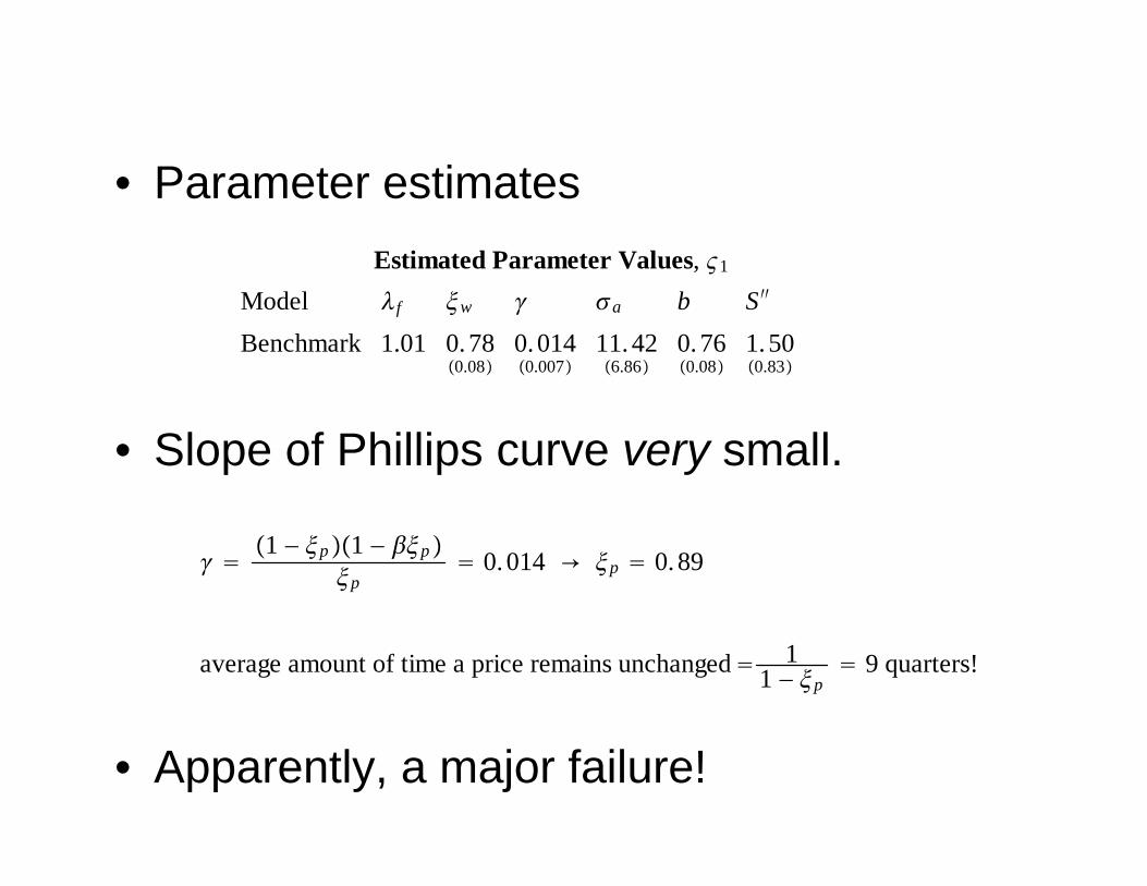
• Slope of Phillips curve very small.Markup parameter goes to unity in estimation, and estimationcriterion is very flat

1 − p1 − p

p 0.014 → p 0.89

criterion is very flat.

average amount of time a price remains unchanged 11 − p

9 quarters!

• Apparently, a major failure!

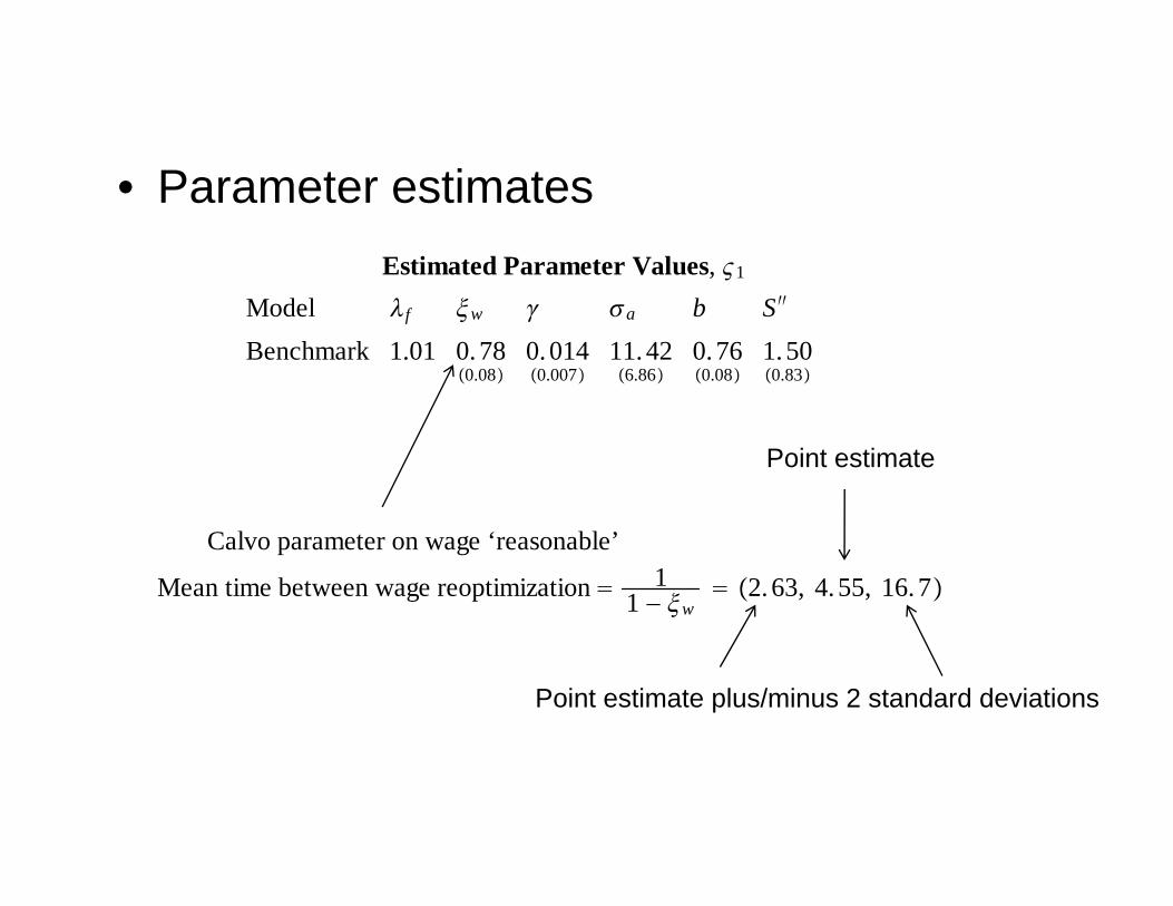
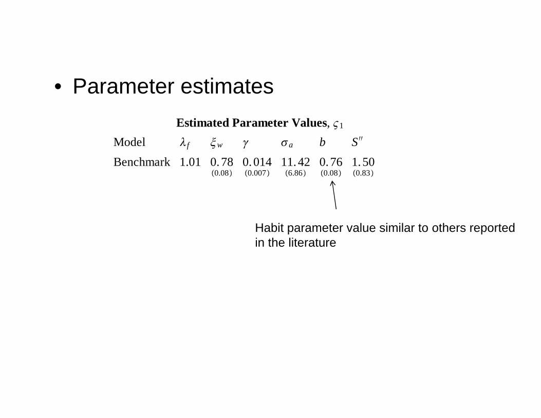
• Parameter estimatesEstimated Parameter Values, 1

Model f w a b S ′′

Benchmark 1.010.080.78

0.0070.014

6.8611.42

0.080.76

0.831.50

0.230.61

• Slope of Phillips curve very small.Point estimate

1 − p1 − p

p 0.014 → p 0.89

Calvo parameter on wage ‘reasonable’

Mean time between wage reoptimization 11 − w

2.63, 4.55, 16.7

average amount of time a price remains unchanged 11 − p

9 quarters!Point estimate plus/minus 2 standard deviations

• Apparently, a major failure!

• Parameter estimatesEstimated Parameter Values, 1

Model f w a b S ′′

Benchmark 1.010.080.78

0.0070.014

6.8611.42

0.080.76

0.831.50

0.230.61

• Slope of Phillips curve very small.A big number, implying capital utilization hardly varies

1 − p1 − p

p 0.014 → p 0.89

A big number, implying capital utilization hardly varies

average amount of time a price remains unchanged 11 − p

9 quarters!

• Apparently, a major failure!

• Parameter estimatesEstimated Parameter Values, 1

Model f w a b S ′′

Benchmark 1.010.080.78

0.0070.014

6.8611.42

0.080.76

0.831.50

0.230.61

• Slope of Phillips curve very small.Habit parameter value similar to others reported

1 − p1 − p

p 0.014 → p 0.89

in the literature

average amount of time a price remains unchanged 11 − p

9 quarters!

• Apparently, a major failure!

• Parameter estimatesEstimated Parameter Values, 1

Model f w a b S ′′

Benchmark 1.010.080.78

0.0070.014

6.8611.42

0.080.76

0.831.50

0.230.61

• Slope of Phillips curve very small.

1 − p1 − p

p 0.014 → p 0.89

average amount of time a price remains unchanged 11 − p

9 quarters!

• Apparently, a major failure!

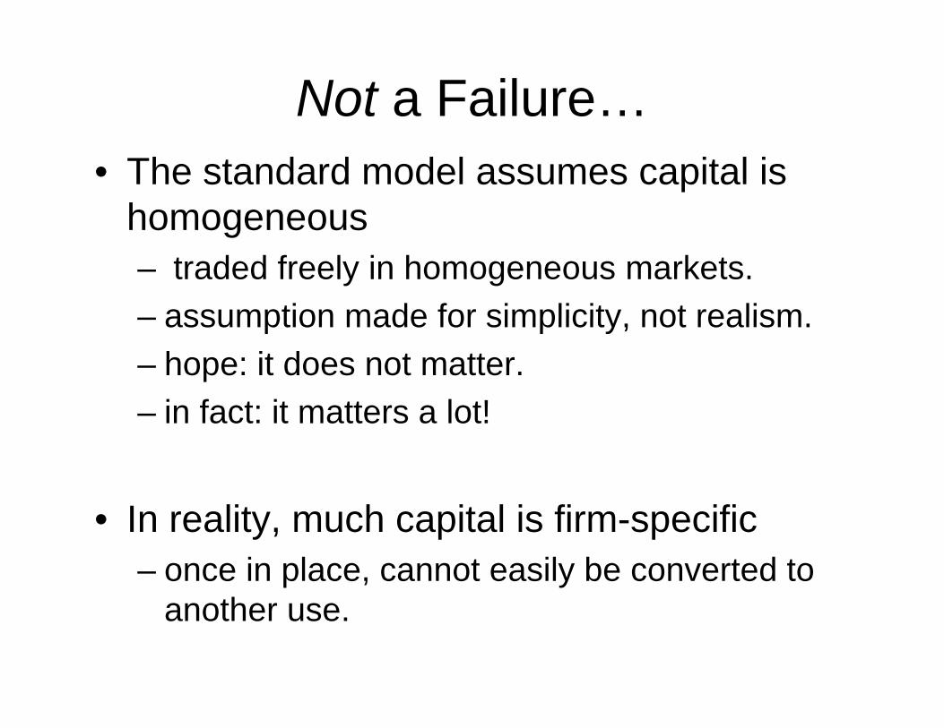
Not a Failure…• The standard model assumes capital is

homogeneoushomogeneous– traded freely in homogeneous markets.– assumption made for simplicity not realism– assumption made for simplicity, not realism.– hope: it does not matter.

in fact: it matters a lot!– in fact: it matters a lot!

• In reality, much capital is firm-specific– once in place, cannot easily be converted to

another use.

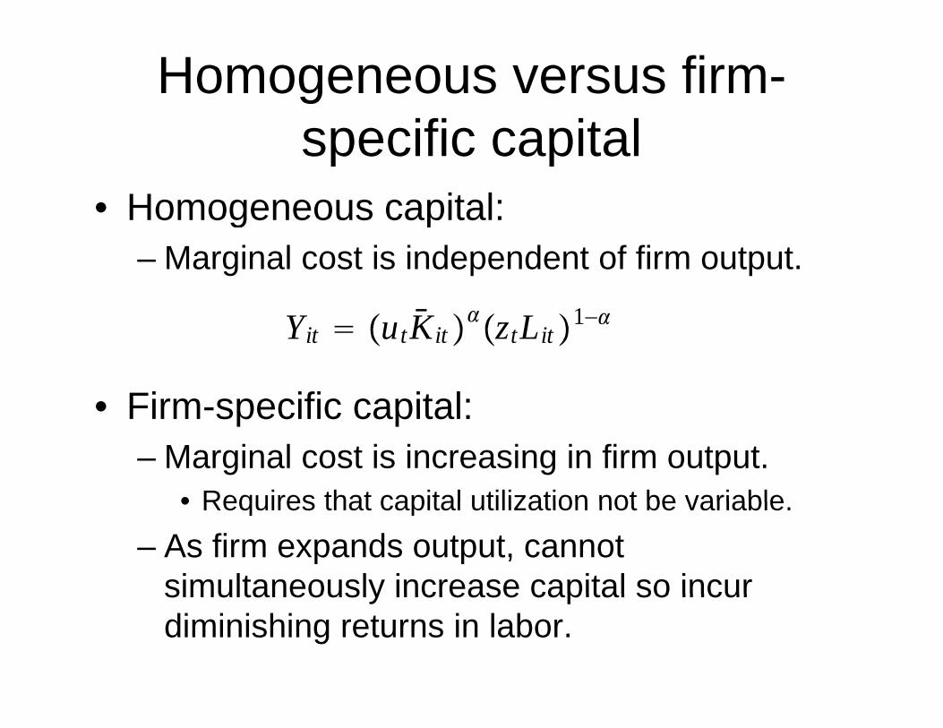
Homogeneous versus firm-specific capitalspecific capital

• Homogeneous capital:g p– Marginal cost is independent of firm output.

Y K L 1−

• Firm-specific capital:

Yit utKit ztLit 1−

• Firm-specific capital:– Marginal cost is increasing in firm output.

• Requires that capital utilization not be variable• Requires that capital utilization not be variable.– As firm expands output, cannot

simultaneously increase capital so incursimultaneously increase capital so incur diminishing returns in labor.

Homogeneous versus firm-specific capital, cnt’d…

Wh fi h i i i l t• When firms have rising marginal cost, a given shock to marginal cost has smaller i t iimpact on price.

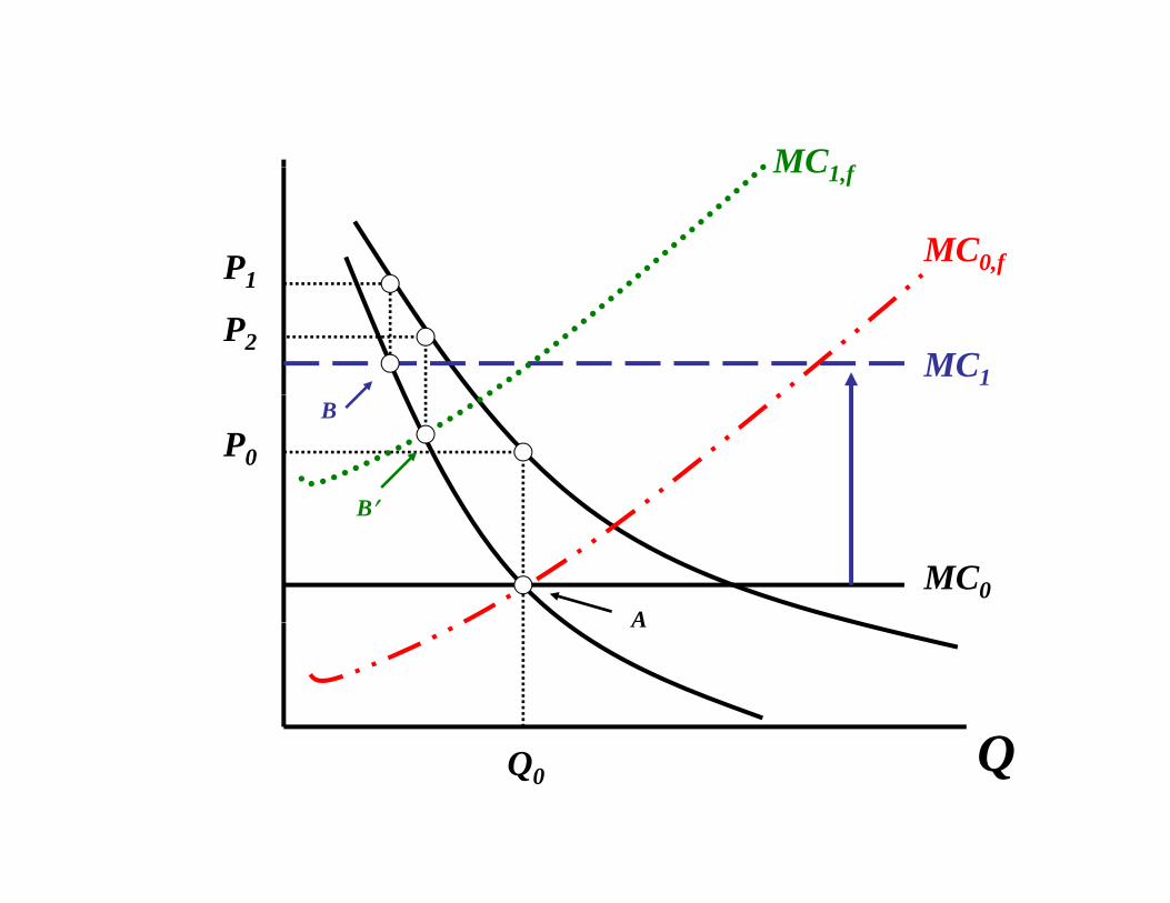
MC1 f

P1MC0,f

MC1,f

1

P2MC1

P0

B

B′

MC0A

B

Q

A

QQ0

More Intuition: Rising Marginal C d I i R i P iCost and Incentive to Raise Price

• A Firm Contemplates Raising Pricep g

– This Implies Output Falls– Marginal Cost Falls– Incentive to Raise Price Falls

• Effect Quantitatively Important When:

– Marginal Cost Steep (capital firm-specific; no variable utilization, large)a

– Demand Elastic (elasticity of demand, ) f

f − 1

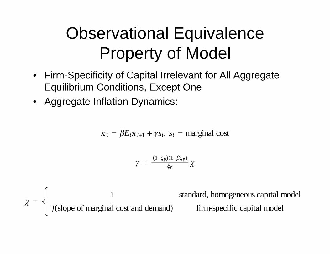
Observational Equivalence P f M d lProperty of Model

• Firm-Specificity of Capital Irrelevant for All Aggregate p y p gg gEquilibrium Conditions, Except One

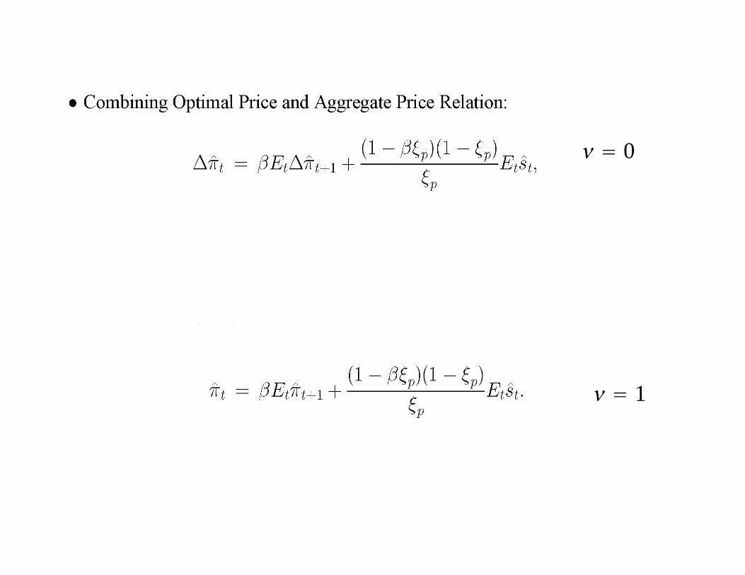
• Aggregate Inflation Dynamics:

t Ett1 st, st marginal cost

1−p1−p

p

1 standard, homogeneous capital model

fslope of marginal cost and demand firm specific capital modelfslope of marginal cost and demand firm-specific capital model

Degree of Price Stickiness in Model with Firm-specific Capital

IMPLIED AVERAGE TIME (Quarters) BETWEEN REOPTIMIZATION1

1−Pelasticity of demand, f

f−1

Model Firm-Specific Capital Model Homogeneous Capital Model demand: Yit Pit

f f−1

constantBenchmark (f 1.01) 1.8 9.4 101f 1.05 3.2 9.1 21f 1.10 4.0 8.8 11f 1.20 4.9 8.3 6

Plausible degree of price stickiness with assumption that capital is firm-specificconsistent with the flat slope of the Phillips curve.

Full assessment requires an estimate of firm-level demand elasticityFull assessment requires an estimate of firm level demand elasticity.

But, is the model consistent with evidence that inflation doesn’t respond much to a monetary policy shock?

Conclusion of Analysis of Standard Model

• Simple model with various frictions isSimple model with various frictions is capable of accounting well for key features of economic responses to monetary andof economic responses to monetary and technology shocks.

• But, model is missing financial frictions, d t b d t dd fand so cannot be used to address many of

the policy questions arising from the fi i l i ifinancial crisis.