Frictions in DSGE Models:

Revisiting New Keynesian vs New Classical Results

Renato FacciniQueen Mary, University of London and Centre for Macroeconomics (LSE)�

Eran YashivTel Aviv University, Centre for Macroeconomics (LSE), and CEPRy

May 8, 2015z

Abstract

We study the interactions of convex hiring and investment frictions and price frictions in a

DSGE model. These turn out to produce major changes in outcomes of all key macroeconomic

variables, shedding new light on New Keynesian vs New Classical results.

We examine technology and monetary shocks under alternative speci�cations of the two

kinds of frictions. While we reproduce the well-known �nding whereby introducing only price

frictions breaks money neutrality and turns the response of employment to technology shocks

from positive to negative, when we add hiring and investment frictions we �nd, inter alia, that:

(i) Introducing even a moderate amount of hiring frictions in the New-Keynesian model

o¤sets the e¤ects of price frictions, making a monetary expansion at least neutral. However this

is not the result of full �exibility but rather of a con�uence of frictions.

(ii) With the cited frictions there is a positive response of employment to technology shocks.

(iii ) A version of the New-Keynesian model, whereby hiring frictions re�ect conservative

estimates of training costs, produces impulse responses to monetary and technology shocks that

are virtually identical to those obtained in the new classical model with the same hiring frictions.

(iv) Interacting price frictions with hiring or investment frictions generates endogenous wage

rigidity by smoothing the response of the marginal rate of substitution between consumption

and labor to shocks.

Keywords: New classical model, New-Keynesian model; hiring and investment frictions, price

frictions; DSGE; business cycles; endogenous wage rigidity

JEL codes: E22, E24, E32, E52

�Email: r.faccini@qmul.ac.ukyEmail: yashiv@post.tau.ac.ilzWe are grateful to seminar participants at the University of Southampton for valuable comments and suggestions

and to Tanya Baron for assistance. Any errors are our own. The graphs in this paper are best viewed in color.

1 Introduction

This paper studies the interaction of convex hiring and investment frictions and price frictions in a

DSGE model. This examination turns out to produce major changes in outcomes of all key macro-

economic variables. Speci�cally, we examine technology and monetary shocks under alternative

speci�cations of the two sets of frictions.

Special cases include the New Classical benchmark with no frictions, and the New-Keynesian

model with only price frictions.

These two dimensions of frictions have been underlying three major strands of literature: price

frictions are the bedrock of New-Keynesian models, which embedded them in DSGE frameworks,

as surveyed by Woodford (2003), Gali (2008) and Christiano, Trabandt and Walentin (2010); labor

frictions lie at the foundations of the search model of Diamond, Mortensen and Pissarides (DMP;

see Pissarides (2000) and Rogerson and Shimer (2011) for surveys); capital frictions underlie the

Tobin�s q literature (see Chirinko (1993) and Smith (2008) for surveys). We model convex price

adjustment frictions following Rotemberg (1982) and labor and capital frictions as convex hiring

and investment costs, following Merz and Yashiv (2007) and Yashiv (2014).

We reproduce the well-known �nding whereby introducing only price frictions breaks money

neutrality and turns the response of employment to technology shocks from positive to negative.

But when we add hiring and investment frictions we �nd that:

(i) Introducing even a moderate amount of hiring frictions in the New-Keynesian benchmark

o¤sets the e¤ects of price frictions, making money at least neutral. However this is not the result

of full �exibility but rather of a con�uence of frictions.

(ii) In this case there is a positive response of employment to technology.

(iii ) A version of the New-Keynesian model, where hiring frictions are calibrated to re�ect

conservative estimates of training costs, produces impulse responses to monetary and technology

shocks that are virtually identical to those obtained in the New Classical model. Investment frictions

also contribute to dampen the mechanism at work in the New-Keynesian model, but for reasonable

parameterizations their impact is not strong enough to restore the classical dichotomy.

(iv) Interacting price frictions with hiring or investment frictions generates endogenous wage

rigidity by smoothing the response of the marginal rate of substitution between consumption and

labor to shocks.

These results are consistent with VAR evidence by Uhlig (2005) who, based on an agnostic

identi�cation scheme, concludes that a monetary stimulus is as likely to increase output as to

decrease it. Moreover, for the same parameter values, the model generates countercyclical marginal

costs conditional on monetary shocks, which is in line with recent evidence by Nekarda and Ramey

(2013) and in contrast with standard predictions obtained in the textbook New-Keynesian model

with a frictionless labor market. Similar analysis on the e¤ects of investment frictions suggests

that these costs also dampen the mechanism at work in the baseline New-Keynesian model, but, as

1

noted, to a lesser extent.

The mechanism governing the interaction between price frictions and hiring and investment

frictions works in two ways:

First, price frictions a¤ect the reaction of hiring and investment to changes in the value of jobs

and capital via the marginal cost. This channel is absent in real models of the labor market, such

as the canonical DMP model, and in Tobin�s Q models, where there is no role for marginal costs.

Second, hiring and investment frictions a¤ect the reaction of hiring and investment to changes

in the marginal cost. This channel is absent in standard New Keynesian models with frictionless

labor and capital markets and o¤sets the mechanism at work in this class of models.

It is worth emphasizing that hiring and investment frictions do not operate trivially by smoothing

the response of hiring and investment. So the results do not follow from the assumption that frictions

in labor and capital markets are large, so quantities cannot respond. Rather, the relative price e¤ect

on capital and job values produces non-trivial dynamics, whereby hiring (and investment) increase

with labor (and capital) frictions. Finally, we show that interacting price frictions with hiring or

investment frictions generates endogenous wage rigidity by smoothing the response of the marginal

rate of substitution between consumption and labor to shocks.

It is also important to emphasize that the results are not a comeback to the New Classical/RBC

approach with a stress on supply and technology shocks, as opposed to demand shocks. First,

the mechanisms in question involve a con�uence of frictions, not �exibility. Second, recent papers

have shown that technology shocks may be the result of demand shocks (see Bai, R¬os-Rull, and

Storesletten (2012)).

The paper is organized as follows. Section 2 presents the model, Section 3 discusses the calibra-

tion and shows impulse responses. Section 4 introduces our examination of the role of each type

of frictions. Section 5 explores the interaction between price frictions and hiring frictions, while

Section 6 investigates the interactions between price frictions and investment frictions. Section 7

concludes.

2 The Model

2.1 The Set-Up

We propose a DSGE model with both hiring and investment frictions, as in Merz and Yashiv

(2007) and Yashiv (2014), and price frictions, as in New-Keynesian models with capital. The

model features three sources of frictions: price adjustment costs, costs of hiring workers and costs

of installing capital. Absent all frictions, the model boils down to the benchmark New Classical

model. Introducing price frictions into the otherwise frictionless model yields the New-Keynesian

benchmark, and introducing hiring or investment frictions over the New-Keynesian benchmark

allows us to analyze how the interplay between these frictions a¤ects the propagation of technology

2

and monetary shocks. In the spirit of simplicity, our modeling strategy deliberately abstracts from

all other frictions and features that are quite prevalent in DSGE models and which are typically

introduced to enhance propagation and improve statistical �t: namely, habits in consumption,

variable capacity utilization, wage rigidities etc.

In what follows we look in detail at households, two types of �rms, the monetary authority and

the aggregate economy.

2.2 Households

The representative household comprises a unit measure of workers searching for jobs in a frictional

labor market. At the end of each time period workers can be either employed or unemployed; we

therefore abstract from participation decisions and from variation of hours worked on the intensive

margin.1 The household enjoys utility from the aggregate consumption index Ct and disutility from

employment, Nt. Employed workers earn the nominal wage Wt and hold nominal bonds denoted

by Bt. Both variables are expressed in units of consumption, which is the numeraire. The budget

constraint is:

PtCt +Bt+1Rt

=WtNt +Bt +�t; (1)

where Rt = (1 + it) is the gross nominal interest rate, Pt is the price of the consumption good

and �t is a lump sum component of income which includes dividends from ownership of �rms and

government transfers.

The labor market is frictional and workers who are unemployed at the beginning of each period

t are denoted by U0t . It is assumed that these unemployed workers can start working in the same

period if they �nd a job with probability xt = HtU0t, where Ht denotes the total number of matches.

It follows that the workers who remain unemployed for the rest of the period, denoted by Ut, is

Ut = (1� xt)U0t . Consequently, the evolution of aggregate employment Nt is:

Nt = (1� �N )Nt�1 + xtU0t ; (2)

where �N is the separation rate.

The intertemporal problem of the households is to maximize the discounted present value of

current and future utility:

maxCt+j

Et

1Xj=0

�j�lnCt+j �

�

1 + 'N1+'t+j

�;

subject to the budget constraint (1) and the law of motion of employment (2). The parameter

� 2 (0; 1) denotes the discount factor, ' is the inverse Frisch elasticity of labor supply and � is a1As shown in Rogerson and Shimer (2011), most of the �uctuations in US total hours worked at business cycle

frequencies are driven by the extensive margin, so our model deliberately abstracts from other margins of variation.

3

scale parameter governing the disutility of work.

Denoting by �t the Lagrange multiplier associated with the budget constraint, the �rst order

necessary conditions and co-states are:

�t =1

PtCt; (3)

1

Rt= �Et

PtCtPt+1Ct+1

; (4)

V Nt =Wt

Pt� �N'

t Ct �xt

1� xtV Nt + � (1� �N )Et

CtCt+1

V Nt+1; (5)

where equation (4) is the standard Euler equation and equation (5) is the marginal value of a job to

the household net of the value of search. This term is equal to the real wage, net of the opportunity

cost of work, �N't Ct, and the �ow value of search for unemployed workers, plus a continuation value.

It is worth noting that relative to the DMP model, where the opportunity cost of work is assumed

to be constant, deriving the net value of employment from a standard problem of the household

implies that this opportunity cost equals the marginal rate of substitution between consumption

and leisure. As we show later in the text, this feature of the model is key in generating endogenous

real wage rigidity in the presence of hiring or investment frictions. It is also worth noting that

in a model with no hiring frictions, where employment generates no rents and thus V Nt = 0, the

marginal rate of substitution equals the real wage: Wt

PCt= �N'

t Ct, which determines labor supply.

2.3 Firms

We assume two types of �rms: intermediate producers and �nal good producers. Intermediate

producers hire labor and invest in capital to produce a homogeneous product, which is then sold

to �nal producers in perfect competition. Final producers transform each unit of the homogeneous

product into a unit of a di¤erentiated product facing price rigidities à la Rotemberg (1982). This

separation between intermediate and �nal goods �rms is often assumed to get around the di¢ culties

that arise whenever the bargaining problem and the price setting decisions are concentrated in the

same �rm. It is assumed that the same bundle of �nal goods is used for consumption and investment

purposes. So output, consumption and investment have the same price, which is denoted by Pt.

Under the common Dixit-Stigliz aggregator of di¤erentiated goods, the expenditure minimizing

price index associated with the output index is

Pt =

0@ 1Z0

Pt (i)1�� di

1A1=(1��)

;

where Pt (i) is the price of a variety i and � denotes the elasticity of substitution.

Intermediate Goods Producers

4

A unit measure of intermediate goods producers sell homogeneous goods to �nal producers

in perfect competition. Intermediate �rms combine physical capital, K, and labor, N , in order

to produce intermediate output goods, Z. The constant returns to scale production function is

f(At; Nt;Kt�1) = AtN�t K

1��t�1 , where At is a standard TFP shock that follows the stochastic process

lnAt+1 = �a lnAt + eat , with e

at � N(0; �a). Following a convention in DSGE modelling, we have

assumed that newly installed capital becomes e¤ective only with a one (quarter) period lag.

It is assumed that hiring and investment are costly activities. We postulate a frictions costs

function g; capturing the di¤erent frictions in the hiring and investment processes. Speci�cally,

we think of hiring costs as the disruption in economic activity associated with worker recruitment.

These costs re�ect training costs, and other costs that are incurred after a worker is hired, and are

not sunk by the time the match is formed. Typically, labor frictions are modelled as vacancy posting

costs, which are sunk at the time of bargaining. As reported in Silva and Toledo (2009) and discussed

in more detail below, training costs are considerably larger than the costs of advertising a vacancy,

and include the time spent by managers and team-workers to instruct new hires, which is a drag

on their ability to produce. Investment involves implementation costs, �nancial premia on certain

projects, capital installation costs, learning the use of new equipment, etc. Both activities may

involve, in addition to production disruption, the implementation of new organizational structures

within the �rm and new production techniques; see Alexopoulos (2011) and Alexopoulos and Tombe

(2012). In sum g is meant to capture all the frictions involved in getting newly employed workers

to work and capital to operate in production, and not, say, just capital adjustment costs or vacancy

costs. All these activities are captured by the friction cost function g(It;Kt�1;Ht; Nt), where I

denotes investment, and H denotes hires.2

These costs are thought of as forgone output. Following Merz and Yashiv (2007) we assume that

the friction cost function is constant returns to scale and is increasing in each of the �rm�s decision

variables.

g(It;Kt�1;Ht; Nt) =

"e12

�ItKt�1

�2+e22

�HtNt

�2#AtN

�t K

1��t�1 : (6)

We assume quadratic costs in line with estimates by Yashiv (2014).3 As shown in Section (3.1), this

convexity implies that large swings in the hiring rates do not imply large deviations of the marginal

hiring cost relative to its steady-state value.

The net output of a representative �rm at time t is:

Zt = f(At; Nt;Kt�1)� g(It;Kt�1;Ht; Nt):2This formulation of frictions/costs is consistent with the Stole and Zweibel (1996) and Cahuc, Marque and Wasmer

(2008) frameworks of intra-�rm bargaining that we use (see in particular the discussion on pages 376-378 and 384-387in the former).

3A rationale for the use of such functional forms, emphasizing consistency of aggregate employment and capitaldynamics with hiring and investment decisions at plant level is provided by King and Thomas (2006) and Khan andThomas (2008), respectively.

5

In every period t, the existing capital stock depreciates at the rate �K and is augmented by new

investment:

Kt = (1� �K)Kt�1 + It; 0 < �K < 1: (7)

Similarly, the number of a �rm�s employees decreases at the rate �N and it is augmented by new

hires Ht. The law of motion for employment reads:

Nt = (1� �N )Nt�1 +Ht; 0 < �N < 1; (8)

which implies that new hires are immediately productive.

At the beginning of each period, �rms hire new workers and invest in capital. Next, wages are

negotiated following standard Nash bargaining. When maximizing its market value, de�ned as the

present discounted value of future cash �ows, the representative producer anticipates the impact of

its hiring and investment policy on the bargained wage. The intertemporal maximization problem

of the �rm reads as follows:

maxEt

1Xj=0

�t;t+j fmct+j [f(At+j ; Nt+j;Kt+j�1)� g(It+j ;Kt+j�1;Ht+j ; Nt+j)]

�Wt+j(It+j ;Kt+j�1;Ht+j ; Nt+j)

Pt+jNt+j � It+j

�;

subject to the laws of motion for capital (7) and labor (8), where �t;t+j = �j CtCt+j

is the real discount

factor of the households who own the �rms andmct � PZt =Pt is the relative price of the intermediate�rm�s good. This relative price equals the real marginal cost for a �nal goods producer since, as

discussed later, producers transform one unit of intermediate good into one unit of �nal good.

The �rst-order conditions for dynamic optimality are:

QKt = Et�t;t+1

��mct+1(fK;t+1 � gK;t+1)�

WK;t+1

Pt+1Nt+1

�+ (1� �K)QKt+1

�; (9)

QKt = mctgI;t +WI;t

PtNt + 1; (10)

QNt = mct (fN;t � gN;t)�Wt

Pt� WN;t

PtNt + (1� �N )Et�t;t+1QNt+1; (11)

QNt = mctgH;t +WH;t

PtNt; (12)

where QKt and QNt are the Lagrange multipliers associated with the capital and the employment

laws of motion, respectively. One can label QKt as Tobin�s Q for capital or the value of capital

and QNt as Tobin�s Q for labor or the value of labor. For an extensive discussion of their economic

signi�cance, see Yashiv (2014).

6

Substituting for QKt and QNt , the four equations above can be rewritten:

mctgI;t +WI;t

PCtNt + 1 = Et�t;t+1

�mct+1(fK;t+1 � gK;t+1)�

WK;t+1

Pt+1Nt+1

+(1� �K)(mct+1gI;t+1 +WI;t+1

Pt+1Nt+1 + 1)

�; (13)

mctgH;t +WH;t

PtNt = mct (fN;t � gN;t)�

Wt

Pt� WN;t

PtNt

+(1� �N )Et�t;t+1�mct+1gH;t+1 +

WH;t+1

Pt+1Nt+1

�; (14)

which o¤er two dynamic equations for the �nal goods producers�real marginal cost.

In a DSGE model with no frictions and no bargaining, equation (14) implies that the marginal

rate of substitution equals the marginal revenue product of employment:

Wt=PCt = mctfN;t

while equation (13) implies that the user cost of capital equals the marginal revenue product of

capital:

EtRt=�t+1 = Et [mct+1fK;t+1 + (1� �K)] :

Final good producers

There is a unit measure of monopolistically competitive �nal good �rms indexed by i 2 [0; 1].Each �rm i transforms Z(i) units of the intermediate good into Y (i) units of a di¤erentiated good,

where Z(i) denotes the amount of intermediate input used in the production of good i. Monopolistic

competition implies that each �nal �rm i faces the following demand for its own product:

Yt(i) =

�Pt(i)

Pt

���Yt; (15)

where Yt denotes aggregate demand from the retailers.

We assume price stickiness à la Rotemberg (1982), meaning �rms maximize current and expected

discounted pro�ts subject to quadratic price adjustment costs.

Final good �rms maximize the following expression:

maxEt

1Xs=0

�t;t+sPtPt+s

"(Pt+s(i)� Pt+smct+s)Yt+s(i)�

�

2

�Pt+s(i)

Pt+s�1(i)� 1�2Pt+sYt+s

#;

subject to the demand function (15). The �rst order conditions with respect to Pt(i) and Yt(i) read

7

as follows:

Yt(i)� ��Pt(i)

Pt�1(i)� 1�

1

Pt�1(i)PtYt = �t"

YtPt

�Pt(i)

Pt

��"�1�Et

��t;t+1

PtPt+1

�

�Pt+1(i)

Pt(i)2

��Pt+1(i)

Pt(i)� 1�Pt+1Yt+1;

�(16)

and

�t = Pt(i)� Pt �mct; (17)

where �t is the Lagrange multiplier associated with eq. (15).

Since all �rms set the same price and therefore produce the same output in equilibrium, equations

(16) and (17) can be combined to obtain the following law of motion for in�ation:

�t(1 + �t) =1� "�

+"

�mct + Et

1

1 + rt(1 + �t+1)�t+1

Yt+1Yt

; (18)

where we have used Et�t;t+1 = 1(1+it)=(1+�t+1)

= 11+rt

, with it and rt denoting the net nominal and

real interest rates, respectively. Equation (18) speci�es that in�ation depends on marginal costs as

well as expected future in�ation. Solving forward equation (18), it is possible to show that in�ation

depends on current and expected future real marginal costs.

2.4 Hiring and Investment Frictions and Marginal Costs

In order to understand the forces driving marginal costs in this model, it is worth solving the FOCs

for capital and employment in equations (9) and (11) formct and Etmct+1, respectively. Rearranging

the dynamic optimality condition for employment in (11), we get the following expression:

mct =

Wt

PCt

fN;t � gN;t+

WN;t

PCtNt

fN;t � gN;t+QNt � (1� �N )Et�t;t+1QNt+1

fN;t � gN;t: (19)

The �rst term in the above equation is the wage component of marginal costs, expressed as

the ratio of real wages to the net marginal product of labor. Because the production function

is Cobb-Douglas, in a no friction model, where gN;t = 0, the wage component is proportional to

the labor share of income WtNt=PtYt. The second term relates to intra-�rm bargaining. Since

the marginal product of labor is decreasing with the size of the �rm, the marginal worker will

decrease the marginal product of labor and the wage bargained by all the intra-marginal workers.

Correctly anticipating the e¤ect of hiring policies on the negotiated wage bill generates an incentive

to increase hiring. In our model, this intra�rm bargaining e¤ect has an impact on the marginal

cost: the marginal cost of expanding output by raising employment, decreases with the negative

e¤ect of �rm size on the negotiated wage bill.

The third term shows that with frictions in the labor market, marginal costs depend on expected

changes in the value of employment, a point already made by Krause, Lopez-Salido and Lubik (2008).

8

Introducing hiring frictions in a standard New Keynesian model implies that the cost of hiring a

marginal worker no longer coincides with the real wage. On top of the wage there are additional

costs re�ecting the disruption of economic activity that is generated by training new hires for their

jobs. Because �rms expand employment up to the point where the present value of a marginal hire

QNt equals the marginal hiring cost, the term that enters the marginal cost equation in (19) equals

the expected change in the marginal hiring cost. So, for instance, an expected increase in marginal

hiring costs translates into lower current marginal costs, re�ecting the savings of future recruitment

costs that can be achieved by recruiting in the current period.

In our model marginal costs are also related to the dynamics of capital. Rearranging equation

(9) to solve for expected real marginal cost next period, one gets the following expression:

Etmct+1 = Et

WK;t+1

Pt+1Nt+1

At+1fK;t+1 � gK;t+1+

1

�t;t+1EtQKt � �t;t+1(1� �K)QKt+1At+1fK;t+1 � gK;t+1

: (20)

The �rst term in equation (20) is a term re�ecting intra�rm bargaining. A higher capital stock

makes workers more productive, thereby increasing the expected marginal product of labor and

the bargained wage. In equation (9), the presence of this term re�ects a typical hold-up problem:

because workers appropriate parts of the rents generated by employment, the capital e¤ect on wages

decreases the value of capital, leading to under-investment. By rearranging equation (9) to solve

for the expected marginal cost, we can look at the e¤ect of capital on wages as a determinant of

real marginal costs: the marginal cost of expanding production by increasing capital rises with the

positive e¤ect of capital on wages.

The second term shows that expected changes in Tobin�s Q for capital (QK) also a¤ect real

marginal costs: the marginal cost of expanding output by increasing capital is netted out of the

expected gains in the value of capital. In analogy with the case of hiring discussed above, the

term QKt re�ects both the marginal value of a unit of capital and the marginal cost of investment.

Hence, the term QKt � �t;t+1(1 � �K)QKt+1 can be interpreted as the expected change in marginalinvestment costs, which is always zero in a model with no investment frictions. Friction costs will

give rise to richer dynamics in the value of capital, which will be driven, as dictated by equation

(10), by changes in marginal investment costs, evaluated in units of forgone output, and by changes

in the impact of investment on the negotiated wage bill.

It is worth noting that hiring and investment frictions interact in general equilibrium. Replacing

(12) into (10) we get:

QKt =QNt �

WH;t

PCtNt

gH;tgI;t +

WI;t

PCtNt + 1;

9

while substituting (10) into (12) we obtain:

QNt =QKt �

WI;t

PCtNt � 1

gI;tgH;t +

WH;t

PCtNt:

Quite clearly, the marginal cost of investing and hiring, which re�ect the existence of frictions as

per equations (10) and (12), directly a¤ect each other.

2.5 Wage Bargaining

Wages are assumed to maximize a geometric average of the household�s and the �rm�s surplus

weighted by the parameter , which denotes the bargaining power of the households:

Wt = argmaxn�V Nt

� �QNt

�1� o; (21)

The �rst order condition to this problem leads to the Nash sharing rule:

(1� )V Nt = QNt : (22)

Substituting (5) and (11) into the above equation and using the sharing rule (22) to eliminate the

terms in QNt+1 and VNt+1 one gets the following expression for the real wage:

Wt

Pt= mct (fN;t � gN;t)�

WN;t

PtNt + (1� )

��CtN

'it +

xt1� xt

1� QNt

�: (23)

Assuming a Cobb-Douglas production function and the frictions cost function in (6), the solution

to the di¤erential equation in (23) reads as follows:

Wt

Pt= mctA

�t K

1��t�1

��

�1� e1

�1

�ItKt�1

��1�A1N

��1t +

�1� �

�2

�e2H

�2t A2N

��1��2t

�

+(1� )��CtN

'it +

xt1� xt

1�

�mctgH;t +

WH;t

PCtNt

��; (24)

where A1 and A2 are parameters, which are reported in the Appendix A together with the full

derivation.

Notice that in the special case in which workers have no bargaining power, i.e., = 0, the real

wage equals the marginal rate of substitution between consumption and leisure, as in the standard

New-Keynesian model with a frictionless labor market.

10

2.6 Aggregation and Equilibrium Conditions

Aggregating output demand implies the following relationship between consumption and investment

demand, and aggregate supply of the �nal good:

Ct + It = Yt =

0@ 1Z0

Yt(i)(��1)=�di

1A�=(��1)

: (25)

Aggregating on the supply side of the economy implies the following relationship between �nal

goods and intermediate inputs:

Zt = f(At; Nt;Kt�1)� g(It;Kt�1;Ht; Nt) = Yt1Z0

�Pt(i)

Pt

���di = Yt; (26)

where

1Z0

�Pt(i)Pt

���di = 1 since with Rotemberg pricing there is no price dispersion in equilibrium.

Combining the expressions in (25) and (26) implies that:

Ct + It = f(At; Nt;Kt�1)� g(It;Kt�1;Ht; Nt): (27)

2.7 The Monetary Authority

The monetary authority sets the nominal interest rate following the Taylor rule:

RtR�

=

�Rt�1R�

��r �� 1 + �t1 + ��

�r� � YtY �

�ry�1��r�t; (28)

where �t measures the rate of in�ation of the numeraire good, and an asterisk superscript denotes the

steady-state values of the associated variables. When linearizing the model around the stationary

equilibrium we will assume that �� = 0. The parameter �r represents interest rate smoothing, and

ry and r� govern the response of the monetary authority to deviations of output and in�ation from

their steady-state values. The term �t captures a monetary policy shock, which is assumed to follow

the process ln�t = ��ln�t�1 + e�t , with e

�t � N(0; ��).

3 Impulse Responses in the Full Model

We start this section by calibrating the full model with price rigidities and with frictions in both

labor and capital markets. This will provide a benchmark for the analysis to follow, namely the

full DSGE model with all frictions. We then compare how the impulse responses of real variables

such as the hiring rate, the investment rate, real wages and net output change when we shut down

11

price frictions and/or frictions in capital and labor markets. In what follows we will look at both

technology and monetary shocks.

We linearize the model around the non-stochastic steady state and solve for the policy functions,

which express the control variables as a function of the states and the shocks. We then shock the

stationary equilibrium of the model with a technological or a monetary innovation, and iterate on

the policy functions and on the laws of motion for the state variables to trace the expected behaviour

of the endogenous variables, i.e., we produce impulse responses.

3.1 Calibration

We calibrate the parameters that a¤ect the stationary equilibrium of the model using two sources

of information: some parameters are either normalized or set using a priori information, while the

remaining ones are selected so as to match U.S. data.

Table 1

The discount factor � equals 0:99 implying a quarterly interest rate of 4%. The quarterly job

separation rate �N is set 0:133 as in the data and measures separations from employment into

either unemployment or inactivity (see Appendix B in Yashiv (2014) for details), while the capital

depreciation rate �K is set to 0:02 to match the US investment to capital ratio. The inverse Frisch

elasticity ' is set equal to 3, in line with the range of estimates by Domeji and Floden (2006) and

in between the value of 5 used in Gali (2010) and the more standard value of 1 as in Christiano

Eichenbaum and Trabant (2013) among many others. The elasticity of substitution in demand

� is set to the conventional value of 11, implying a steady-state markup of 10%, consistent with

estimates presented in Burnside (1996)and Basu and Fernald (1997). Finally, the scale parameter

� in the utility function is normalized to equal one.

This leaves us with four parameters to calibrate: the elasticity of output to the labor input

�, the bargaining power and the two scale parameters in the friction costs function, e1 and e2.

These four parameters are calibrated to match: i) a labor share of 2/3;4 ii) a ratio of marginal

hiring friction costs to the average product of labor, gH=(f=N), equal to 0.20, which corresponds to

nearly one month of wages; iii) a ratio of marginal investment friction costs to the average product

of capital, gI= (f=K), equal to 0.80; iv) total friction costs around 2% of output. Our calibration

of costs is conservative in the sense that the target values for total and marginal frictions costs lie

at the low part of the spectrum of estimates reported in the literature; we discuss this below. The

unemployment rate implied by the calibration is approximately 12%. This value is in line with the

average of the time series for unemployment rates produced by the BLS designed to account for

4 In this model the elasticity of output to the labor income does not correspond exactly to the labor share of income,but these two values are close at the calibrated stationary equilibrium.

12

workers who are marginally attached to the labor force (U-6), consistently with our measure of the

separation rate.5

Our calibration of labor frictions merits discussion. The papers of Krause, Lopez-Salido and

Lubik (2008) and Gali (2010) assume that average hiring costs equal nearly 5% of quarterly wages,

following empirical evidence by Silva and Toledo (2009) on vacancy advertisement costs. Our

functional form for friction costs �discussed extensively in Yashiv (2014) �allows for hiring costs

to be interpreted in terms of training costs as well as all other sources of forgone output associated

with hiring and discussed in Section 2.3. As reported by Silva and Toledo (2009), average training

costs are about 55% of quarterly wages, a �gure that is nearly ten times as large as that of vacancy

posting costs. In our calibration we follow the estimates in Yashiv (2014) and prefer to err on the

conservative side: the calibration target for marginal hiring friction costs in point (ii) above implies

a ratio of gH= (W=P ) around 30%, nearly one month of wages. Note that the hiring rate Ht=Nt in

the data is in the interval [0:114; 0:161] in the period 1976Q1-2011Q4. Hence the ratio of marginal

hiring costs over steady state wages gHW=P ; using our calibration values, ranges between 26% and

37% of quarterly wages. This represents relatively little variation and an upper bound that is well

below the average training cost reported by Silva and Toledo (2009).6 The Rotemberg parameter

governing price stickiness is set to 120, to match a slope of the Phillips curve of 0.1, as implied by

Gali�s (2010) calibration.7 As for the technology shocks, we assume an autocorrelation coe¢ cient

�a = 0:95, while monetary shocks are assumed to be i.i.d.

3.2 Impulse Responses

Technology Shocks

Figure 1 plots the impulse responses to a positive technology shock in the following four versions

of the model: (i) the model with all the frictions � the New-Keynesian model embodying price

frictions together with hiring and investment frictions (discussed in the calibration above); (ii) the

New Classical model with both capital and labor frictions; this is obtained by setting a very low

level of price frictions, i.e. � ' 0, while maintaining hiring and investment frictions as in the baselinecalibration; (iii) the standard New Keynesian model obtained by maintaining a high degree of price

rigidities, i.e. � = 120, but setting capital and labor frictions close to zero, i.e. e1 ' 0 and. e2 ' 0;(iv) the standard New Classical model with no frictions obtained by setting � ' 0, e1 ' 0 and

e2 ' 0.5BLS series can be downloaded at: http://data.bls.gov/pdq/SurveyOutputServlet6The ratio gH

W=Pimplied by the functional form in (6) is computed as e2

�HN

� �KN

�1��= (W=P ), for di¤erent values

of H=N assuming WPand K

Nremain constant at their steady state values.

7Our value for � is obtained by matching the same slope of the Phillips Curve as in Gali: �"=(1��p)(1���p)

�p,

where �p is the Calvo parameter. Notice that for given " and �, this equation implies a unique mapping between �pand �. While Gali (2010) assumes Calvo pricing frictions, with �p = 0:75, we adopt Rotember pricing frictions, whichimplies that in our speci�cation prices are e¤ectively reset every quarter.

13

Figure 1

The �gure shows that the impulse responses of hiring, employment, investment, capital and

output are virtually identical in the two models with hiring and investment frictions (models i

and ii above; the green and blue lines in the �gure); this implies that in the presence of hiring

and investment frictions, the response of these real variables is independent of the level of price

rigidities.

Upon impact of the technology shock, the response of hiring, employment and output in the

standard New-Keynesian benchmark (model iii, the red line) is markedly di¤erent with respect to

all other models. Employment contracts substantially in this model, which attenuates materially

the response of output. Because the job separation rate is very high at quarterly frequencies, the

impact of the technology shock on employment is quickly reabsorbed after the �rst period, implying

that the dynamics of the responses beyond the �rst quarter are broadly similar across models.

Interestingly, adding hiring and investment frictions onto the New Keynesian benchmark generates

a smoother reaction in real wages, meaning that frictions generate endogenous wage rigidity.

In the New Classical model with no or little frictions (model iv, the black line) the impulse

responses are the usual RBC responses with employment, capital and output increasing following a

positive technological innovation.

Monetary Shocks

Figure 2 plots impulse responses to an i.i.d. expansionary monetary shock in the same four

versions of the model discussed above.

Figure 2

The results show that in the absence of price rigidities, money is neutral, independently of the

presence of frictions in labor and capital markets. In the New-Keynesian benchmark (model iii)

instead, the monetary shock has real e¤ects, but these e¤ects do not last for long, as the model

lacks propagation.

Most importantly, real variables respond very di¤erently in the New-Keynesian model with

(model i) and without (model iii) hiring and investment frictions: introducing these frictions virtu-

ally eliminates all real e¤ects of monetary shocks, so that the response of the New-Keynesian model

with hiring and investment frictions is virtually indistinguishable from the response of the New

Classical benchmark. The ine¤ectiveness of monetary policy to stimulate output is consistent with

VAR evidence by Uhlig (2005) who, under agnostic identi�cation assumptions, �nds that following

a monetary stimulus, output is just as likely to increase as to decrease.

The results above imply that either hiring or investment frictions or their coexistence, neutralize

the impact of price frictions on the propagation of technological and monetary shocks. In what

follows we elucidate the role of both frictions in the propagation of shocks.

14

4 Exploring Price Frictions vs. Hiring and Investment Frictions

We aim to study the role of price frictions, such as those underlying New Keynesian models, vs. the

role of labor frictions, such as those underlying search models, and capital frictions, such as those

underlying Tobin�q investment models. We thus take the New Classical model (NC) as a friction-

less benchmark. We then ask what is the e¤ect of introducing price frictions and of introducing

labor or capital frictions into the model. We do so by :

(i) Varying the value of the parameter governing price adjustment costs, �; and looking at the

e¤ect of shocks upon impact on the hiring (HtNt ) and investment (It

Kt�1) rates, on real wages (Wt

PCt),

and on net output (ft � gt). We denote the resulting e¤ect by New Keynesian �NK.�(ii) Varying the value of the parameter governing labor frictions, e2; and looking at the e¤ect

of shocks upon impact on the same variables. We denote the resulting e¤ect by �L frictions.�

(iii) Varying the value of the parameter governing capital frictions, e1; and looking at the e¤ect

of shocks upon impact on the same variables. We denote the resulting e¤ect by �K frictions.�

(iv) Varying the value of both �; and e1 or e2 together and looking at the e¤ect of shocks upon

impact. We denote the resulting e¤ect by �NK+ L frictions�or �NK+ K frictions.�

Using 3D graphs with the relevant parameters variation on two axes and the a¤ected variable

on the third axis, we attempt to explain the mechanisms underlying the results.

In the next two sections, we analyze the response of cited variables to technology and to monetary

shocks, under these model variations. One aspect of the analysis to note is that we present graphs

featuring reasonable ranges of parameter values. The reader can choose a region in the 3D space

conforming to his/her own priors to gauge the results. Thus, while we indicate four points in this

space, corresponding to the models under review, these are just reference points and the graphs

o¤er a �bigger picture.�

In general, before going into the speci�c analyses, we note the following: price frictions introduce

a key role for marginal costs, which serve as a relative price here mct � PZt =PCt ; they engender

responses of real variables � hiring, investment and the real wage � given the �rm�s inability to

fully and freely adjust prices. Labor (capital) frictions operate to modify the responses of hiring

(investment) rates through convex costs functions.

Considering both sets of frictions together, we �nd that the labor and capital frictions o¤set

price frictions, bringing the total e¤ects closer to the frictionless benchmark. This works in two

ways:

(i) The existence of price frictions (the role of mct) alters the response of �rms� hiring and

investment to the value of jobs (QNt ) and of capital (QKt ).

(ii) Concurrently, the presence of labor and capital frictions a¤ects the response of hiring and

investment to changes in the relative price (changes in mct).

Note that hiring and investment frictions do not operate trivially by smoothing the response of

hiring and investment. The results do not follow from the assumption that frictions in labor and

15

capital markets are large, so quantities cannot respond. Rather, the relative price e¤ect on capital

and job values produces non-trivial dynamics, whereby hiring (and investment) increase with labor

(and capital) frictions.

These mechanisms generate non-trivial outcomes such as: (i) �New Classical outcomes� even

with price rigidities; (ii) endogenous wage rigidity (by smoothing the response of the marginal

rate of substitution between consumption and labor to shocks; (iii) much smaller real e¤ects for

monetary policy (due to dampening mechanisms). These are not the result of full �exibility but

rather of a con�uence of frictions.

The following two sections go into the details of these interactions between the two types of

frictions.

5 Interactions Between Hiring Frictions and Price Frictions

This section explores the mechanism underlying the interaction between hiring frictions and price

frictions. For this purpose we consider a version of the model that restricts investment frictions to

be close to zero, i.e., we set e1 ' 0, and examine how the impulse responses change on the impactof technology and monetary shocks for di¤erent parameterizations of price frictions � and hiring

frictions e2. All other parameter values remain �xed at the calibrated values reported in Table 1.

We then illustrate the mechanics of the model by referring to key equations.

We plot impulse responses (see �gures 4 and 6 below) to technology and monetary shocks for

four variables: hiring rates, investment rates, real wages and output. For each variable, we look at

how the response on impact changes as we change the parameters governing price frictions, �, and

hiring frictions, e2. The area colored in blue (red) denotes the pairs of (�; e2) for which the impulse

response is positive (negative). Each point in the �gure marks four benchmark calibrations: the

New Keynesian benchmark with hiring frictions, featuring high price frictions and moderate hiring

frictions, i.e. � = 120 and e2 = 1:5; the New Classical benchmark with hiring frictions, featuring

no price frictions, � ' 0, and moderate hiring frictions, e2 = 1:5, implying that marginal hiring

costs are equivalent to about one month of wages; the New-Keynesian benchmark, featuring high

price frictions and no hiring frictions, i.e. � = 120 and e2 ' 0; and the New Classical benchmark,obtained by restricting price and hiring frictions to values close to zero, i.e. � ' 0 and e2 ' 0. Inthe �gures, colored points are used to emphasize these four benchmark parameterizations.

To understand the transmission of both technology and monetary shocks in the presence of

hiring frictions only, it is crucial to understand what drives the hiring decision. For this purpose it

is useful to rewrite equation (12), solving for the e¤ective job value expressed in units of intermediate

goods: gQNtmct

= gH;t (29)

where

16

gQNt � QNt � WH;t

PCtNt;

= mct (fN;t � gN;t)�Wt

Pt� WN;t

PtNt + (1� �N )Et�t;t+1QNt+1 �

WH;t

PtNt,

and the last equality follows by replacing QNt using equation (11). Substituting this expression forgQNt into (29) we get:mct (fN;t � gN;t)� Wt

Pt� WN;t

PtNt � WH;t

PtNt + (1� �N )Et�t;t+1QNt+1

mct= gH;t: (30)

The LHS are current �ow pro�ts (mct (fN;t � gN;t) � WtPt� WN;t

PtNt � WH;t

PtNt) and the expected

present value of future pro�ts ((1 � �N )Et�t;t+1QNt+1). These are divided by the relative price

mct: The RHS are marginal hiring friction costs. Note that because the marginal hiring cost on the

RHS is linearly increasing in the hiring rate, an increase or decrease in the LHS will translate into

a similar response in the hiring rate. We shall use this representation in what follows.

5.1 E¤ects of Technology Shocks

Before we turn to the analysis of the four speci�c cases discussed above, it is worth looking at how

the response of marginal costs on impact changes with price and hiring frictions (Figure 3).

Figure 3

With a positive technology shock marginal costs mct =PZtPCt

fall as the net marginal product of

labor increases (see equation 19). Only in the special case where prices are fully �exible relative

prices don�t move. The higher are price frictions the stronger is the fall in marginal costs, while

labor frictions have a negligible impact. The role of price frictions is thus expressed strongly through

changes in the marginal costs, which are relative prices.

Figure 4

The New Classical Benchmark

The e¤ective job value (LHS of equation (30)) goes up because mct does not change, and gQNt(the numerator) goes up, driven by higher current and future fN;t: Hence the hiring rate goes up.

The response of the investment rate is positive as fK;t+1 rises with little changes in other variables

in equation (9). Output rises as productivity and employment rise and �nally, real wages go up

as the marginal product of labor, fN;t, and the marginal rate of substitution, �tCtN't , go up (see

equation 23).

The New Classical Model with Labor Frictions

17

This is a very similar case to the preceding one, but higher labor frictions now generate a slightly

weaker response of hiring. Employment increases by less, dampening the response of real wages via

the marginal rate of substitution �tCtN't , and the response of investment via the marginal product

of capital, due to complementarities in the production function. A slightly smaller increase in hiring

and employment implies that also output increase a little less. The lower rise in investment does

not contribute to the explanation why output rises by less on impact since output depends only on

the previous period stock of capital.

The New Keynesian Benchmark

The e¤ect of technological shocks on hiring is the result of two contradictory forces: the direct

(positive) e¤ect of At on productivity and the present value of the jobgQNt , and the indirect (negative)e¤ect that goes through the response of marginal costs. It turns out that the latter dominates and

hiring declines.

To understand the partial e¤ect of technology on hiring that goes through the endogenous

response of marginal costs, it is worth focusing on the product of the elasticities: the total elasticity

of marginal costs with respect to technology shocks �mct;eat , and the partial elasticity of the hiring

rate with respect to marginal costs �HtNt;mct

. Because the former is virtually independent of e2 (see

Figure 3), we can get the intuition for the result by focusing on the latter.

Substituting for gH;t using the functional form in equation (6), we can rewrite equation (30) as

follows:HtNt

=mctBt � Ct

mct

1

e2At (Kt�1=Nt)1�� ;

where Bt � fN;t � gN;t and Ct � WtPt+

WN;t

PtNt � (1� �N )Et�t;t+1QNt+1 +

WH;t

PtNt. We can then use

the above equation to work out the partial derivative of hiring rates with respect to marginal costs,

@HtNt@mct

=mct (fN;t � gN;t)�gQNt

mc2t

1

e2At (Kt�1=Nt)1�� ; (31)

where we have used gQNt � mctBt � Ct. Note that the associated elasticity is �HtNt;mct

=@HtNt

@mct� mctHt

Nt

:

Because the value of a job, gQNt approaches zero as labor frictions decrease, i.e. as e2 ! 0,

and because fN;t � gN;t > 0, the elasticity �HtNt;mct

is positive. Given that marginal costs fall with

positive technology shocks, the partial e¤ect of technology on hiring that goes through marginal cost

is negative. This is the standard mechanism at work in New Keynesian models: because output is

demand driven with price rigidities, an increase in productivity implies that less input is needed to

meet demand, so employment must fall. The fall in hiring needed to meet demand is proportional

to the marginal revenue product. When e2 ' 0 this e¤ect is stronger than the direct e¤ect of

technology on the marginal product of labor, which tends to increase the present value of the job.

Hence the response of both hiring and employment is negative.

18

We now turn to discuss the response of the other real variables reported in Figure 4. Real wages

go down as mct and �tCtN't fall; investment rises, but by much less as employment falls, so by

the complementarities in the production function the marginal product of capital increases by less;

output rises but not by much as in the New Classical benchmark because hiring (and therefore

employment) falls.

New Keynesian model with labor frictions and price frictions

As hiring frictions increase, the rent associated with a �lled job increases, hencegQNt in equation(31) rises, decreasing the elasticity of hiring to marginal costs �Ht

Nt;mct

. This e¤ect derives from

interacting price and hiring frictions, and re�ects the impact of relative prices (mct) on the value

of a job in units of intermediate goods (the LHS of (29)). Whether this e¤ect will be su¢ cient to

overturn the sign of the response of hiring is a numerical question. It turns out that at the calibrated

equilibrium, for parameterizations of labor market frictions that re�ect conservative estimates of

training costs, the response of hiring turns positive on the impact of technology shocks.

The increase in employment implies that wages fall by less than in the New Keynesian model

with a frictionless labor market; the e¤ect of employment on the marginal rate of substitution

endogenously dampens the reaction of real wages. It is also worth noting that for values of �

around 60, which map into a Calvo price stickiness of 2 � 212quarters,8 increasing e2 can turn the

response of real wages to technology shocks from negative to positive, that is, it reproduces the

qualitative response that we observe in a New Classical benchmark. Investment rises substantially;

as hiring rates increase with higher labor market frictions e2; the marginal productivity of capital

rises. Finally output rises substantially as productivity and employment rise.

In summary, as Figure 4 shows, adding labor (hiring) frictions to price frictions brings the New

Keynesian model closer to the results of the New Classical model with labor frictions, i.e., o¤sets

to a signi�cant extent the e¤ects of price frictions.

5.2 E¤ects of Monetary Shocks

With a monetary expansion mct =PZtPCt

rises as the labor share increases. The mechanism is as

follows: a fall in the nominal rate engenders a fall in the real rate that stimulates consumption and

investment. In order to meet the increase in output demand, the demand for labor rises, so the real

wage increases, and in turn this increases the real marginal costs through the rise in labor share.

Before we start discussing the four benchmark cases it is worth inspecting how the impact

elasticity of marginal costs to monetary shocks changes with price frictions and hiring frictions.

Figure 5

Figure 5 shows that only in the special case where prices are fully �exible marginal costs do not

respond. The response of marginal costs increases with price frictions � and is virtually independent8See footnote 6.

19

of hiring frictions e2.

Figure 6

The New Classical Benchmark

The present value of the job does not change as basically nothing moves in the hiring equation

(30). Likewise, real wages, investment and output do not change. This is an expression of money

neutrality.

The New Classical Model with Labor Frictions

Because marginal costs do not respond to monetary shocks, money is still neutral.

The New-Keynesian Benchmark

The e¤ective job value rises and the e¤ect on hiring rates is quantitatively substantial. This is

so as marginal costs respond to monetary shocks and the elasticity of hiring rates to marginal costs

�HtNt;mct

is positive when employment relationships generate no rent (the numerator in the RHS of

equation (31) is positive asgQNt approaches zero for e2 ! 0). The response of the other real variables

follows: real wages rise as mct and �tCtN'it rise; the response of the investment rate is positive as

the marginal cost rises and the marginal product of capital increases with employment; output rises

when hiring rates and employment rise.

The New-Keynesian Model with Labor Frictions

As e2 rises, the value of a jobgQNt increases and the elasticity of hiring to marginal costs �HtNt;mct

falls (see equation (31)). At the calibrated equilibrium, for reasonable parameterizations of hiring

frictions, the elasticity of hiring rates to marginal costs switches from positive to negative, implying

that monetary stimuli could even be contractionary. Under the assumption of hiring frictions equal

to roughly one month of wages, hiring is neutral, i.e., does not respond to monetary policy. Note

that this is not the result of �exibility but rather of a con�uence of frictions. As a consequence,

the real wage response is muted relative to the benchmark New Keynesian model, as the marginal

rate of substitution does not respond as much. Thus labor frictions generate endogenous real wage

rigidity by containing movements in the marginal rate of substitution. Because employment does

not respond with moderate hiring frictions, the productivity of capital remains unchanged, hence

investment does not respond. Output also remains unchanged and money is neutral.

Typically, as noted above, New Keynesian models with search frictions calibrate hiring frictions

to match vacancy posting costs (see Krause, Lopez-Salido and Lubik (2008) and Gali (2010)). These

costs are very small, equivalent to about one week of wages.

Figure 6 recovers Gali�s (2010) result that the performance of the New Keynesian model is

virtually independent of hiring frictions, but this conclusion holds true only in the special case

where the labor market is nearly frictionless. Importantly, what Figure 6 also shows is that for

tiny parameterizations of hiring frictions, the elasticity of hiring rates to marginal costs is very

20

sensitive to the precise level of frictions. Calibrating hiring frictions to match training costs, which

are an order of magnitude higher than vacancy posting costs, would imply selecting values for e2that are larger than 1.5. In this region of the parameter space, a monetary stimulus reduces both

employment and capital as well as output. As a result, marginal costs, conditional on monetary

shocks, become countercyclical, in line with empirical evidence by Nekarda and Ramey (2013), and

in contrast to the predictions of the baseline New Keynesian model with a frictionless, or nearly

frictionless, labor market.

6 Interactions Between Investment Frictions and Price Frictions

This section explores the mechanism underlying the interaction between investment frictions and

price frictions. For this purpose we consider a version of the model that restricts hiring frictions to

be close to zero, i.e. we set e2 ' 0, and examine how the impulse responses change on the impact oftechnology and monetary shocks for di¤erent parameterizations of price frictions � and investment

frictions e1. All other parameter values remain �xed at the calibrated values reported in Table 1.

In Figures 8 and 10 we plot impulse responses to technology and monetary shocks for the same

four variables as before, marking again the same four benchmark parameterizations: the New Key-

nesian benchmark with investment frictions, featuring high price frictions and moderate investment

frictions, i.e. � = 120 and e1 = 40; the New Classical benchmark with investment frictions, featuring

no price frictions, � ' 0, and moderate investment frictions, e1 = 40, implying the same ratio of

marginal investment costs to the marginal product of capital as in the calibration discussed in Sec-

tion 3.1; the New-Keynesian benchmark, featuring high price frictions and no investment frictions,

i.e. � = 120 and e1 ' 0; and the New Classical benchmark, obtained by setting investment and

price frictions close to zero, i.e., � ' 0 and e1 ' 0:To understand the investment decision, rearrange equation (10) to solve for the relevant capital

value expressed in units of intermediate goods

gQKtmct

= gI;t; (32)

where gQKt can be expressed as follows by making use of equation (9):

gQKt = QKt � WI;t

PtNt � 1

= Et�t;t+1

��mct+1(fK;t+1 � gK;t+1)�

WK;t+1

Pt+1Nt+1

�+ (1� �K)QKt+1

�� WI;t

PtNt � 1:

21

Replacing the above expression into equation (32) yields:

Et�t;t+1

h�mct+1(fK;t+1 � gK;t+1)� WK;t+1

Pt+1Nt+1

�+ (1� �K)QKt+1

i� WI;t

PCtNt � 1

mct= gI;t: (33)

We shall use this equation in what follows.

6.1 E¤ects of Technology Shocks

Figure 7 shows that the total elasticity of marginal cost to technology shocks �mct;eat is negative

and increasing (in absolute value) with price frictions �. Only in the special case where prices are

fully �exible does the marginal cost not respond. Also, for relatively high values of price rigidities,

investment frictions reduce the elasticity of marginal cost.

The New Classical Benchmark

The present value of investment (LHS of equation (33)) goes up because marginal costs are

una¤ected, andgQKt (the numerator) goes up, due to higher current and future fK;t: Hence a positivetechnology shock, raises investment: the RHS of equation (33), gI;t, increases linearly with It

KtThe

response of the hiring rate is positive as fN;t+1 rises with the technology neutral shock. Real wages

go up as fN;t and �tCtN'it (the MRS term) go up. Output rises as hiring rates and employment

rise.

The New Classical Model with Capital Frictions

Basically this case is similar to the preceding one with some mitigation of the investment response

due to frictions.

The New Keynesian Benchmark

The response of the investment rate depends on two contradictory forces: the direct (positive)

impact of technology that goes through the marginal product of capital, as described above, and

the indirect (negative) e¤ect that goes through the response of marginal costs. To understand this

second e¤ect, it is convenient to solve equation (33) for the investment rate, after replacing gI;t with

the functional form given by equation (6):

ItKt�1

=Et�t;t+1

h�mct+1(fK;t+1 � gK;t+1)� WK;t+1

Pt+1Nt+1

�+ (1� �K)QKt+1

i� WI;t

PtNt � 1

mct

1

e1AtN�t K

��t�1

The mechanism by which shocks a¤ect investment rates via the response of marginal costs can be

broken down into (i) the e¤ect of investment rates on the change in current marginal costs mct;

and (ii) the response of investment rates to expected marginal costs next period, Etmct+1:

@ ItKt�1

@Etmct+1=Et�t;t+1(fK;t+1 � gK;t+1)

mc21

e1AtN�t K

��t�1

> 0 (34)

22

@ ItKt�1

@mct=�gQKtmc2

1

e1AtN�t K

��t�1; (35)

The expression in equation (34) captures the standard mechanism at work in New Keynesian

models: because output is demand driven when prices are sticky, lower levels of factors of production

are required to meet the demand, hence investment rates fall with (future expected) marginal costs.

The expression in equation (35), instead captures the interaction of investment frictions with

price frictions. Note that it is zero when e1 ' 0 and thus gQKt ' 0; for the current case.Coming back to the two e¤ects together, when e1 ' 0 the direct impact of technology on

investment through the marginal product of capital is quantitatively stronger than the indirect

e¤ect that goes through the response of marginal costs. As a result, investment increases.

The response of the hiring rate is negative because with the labor market being frictionless,

the numerator in equation (31) is positive, so hiring rates and marginal costs move in the same

direction. Finally, real wages go down as mct and �tCtN'it fall and output rises but not by much as

hiring (and therefore employment) falls.

The New Keynesian Model with Capital Frictions

Investment rises, as in the New Keynesian baseline case just described, driven by the increase in

the marginal product of capital. Indeed, investment rises by more, relative to the New Keynesian

model with frictionless capital markets, because higher investment frictions (a higher gQKt ) o¤setthe negative impact of technology on investment that goes through (next period) marginal costs

(compare equations 34 and 35); this is a relative price e¤ect on the value of capital produced by the

interaction between price and investment frictions. So this mechanism tends to o¤set the baseline

mechanism at work in New-Keynesian models.

The e¤ective present value of the job declines, just as in the baseline New Keynesian case, so

the hiring rate falls. However, the fall is less marked because investment rates rise by more, which

increases fN;t. Finally, real wages decline; frictions make the response of employment muted; in

this case employment decreases by less than in the New Keynesian model with frictionless capital

markets, hence real wages fall by less (through the MRS term). Output rises, as in the New

Keynesian model with a frictionless capital market, but by more, as the fall in hiring and hence

employment is less pronounced.

To sum up, the qualitative response of the four real variables above is the same in the New

Keynesian model with and without investment frictions. Quantitatively, the responses in the New

Keynesian model get closer to the ones in the New Classical benchmark as investment frictions rise,

but only by a limited amount.

6.2 E¤ects of Monetary Shocks

The New Classical Benchmark with or without Capital Frictions: the marginal cost does not re-

spond, so money is neutral.

23

The New Keynesian Benchmark : Marginal costs increase with price frictions. The e¤ective

present value of the job and capital value rise, and the e¤ect on both hiring rates and investment

rates is positive and quantitatively substantial. This is so as the elasticity of both hiring rates and

investment rates to marginal costs is positive and strong when employment and capital generate no

rent. Real wages increase as both the marginal cost and the marginal rate of substitution increase.

Output increases re�ecting the increase in hiring and employment.

The New Keynesian Model with Capital Frictions: Investment frictions decrease the elasticity

of investment rates to marginal costs � ItKt�1

;mct(see equation (35)), so investment increases by less.

As a result the value of the job increases by less, implying lower hiring and employment relative to

the case without investment frictions. A relatively lower level of employment implies a relatively

lower increase in the marginal rate of substitution and in real wages. For the same reason, also

output increases by less.

To sum up, investment frictions reduce the e¤ectiveness of a monetary stimulus, but not enough

to make it totally ine¤ective or to reverse the impact it has in the frictionless benchmark.

7 Conclusions

We have shown that the transmission mechanism of technology and monetary shocks in DSGE

models critically hinges upon hiring frictions and, to a lesser extent, on investment frictions. Most

of the empirical research in this �eld has focused on measuring price rigidities, under the common

belief that this is a necessary statistic to gauge the strength of the New-Keynesian mechanism. Our

results indicate that if hiring frictions are strong enough, the precise degree of price rigidity is less

relevant, if not irrelevant, in the propagation of shocks. Therefore, a correct assessment of hiring

costs is key in the calibration of DSGE models.

This paper suggests that for reasonable parameterizations of the model, expansionary monetary

policy is neutral if not contractionary. This raises the question whether the mechanism at work

in New Keynesian models is not e¤ective, and possibly money matters through other channels or

re�nements of the baseline mechanism, or whether money is in fact neutral and, as Uhlig (2005)

posits, identifying assumptions on VARs are selected so as to con�rm our priors on the e¤ectiveness

of monetary stimuli.

The focus of this paper is on understanding how hiring and investment frictions a¤ect the

propagation of shocks to real variables in DSGE models with price rigidities. The next obvious

question to address is what are the implications of these frictions for in�ation dynamics. We

tackle this issue in separate work, where we also take the model to the data and carry out model

comparisons to see what speci�cation of the model is most likely to have produced the data, given

a common set of priors on parameter values.

24

References

[1] Alexopoulos, M. (2011). �Read All About It! What Happens Following a Technology Shock,�

American Economic Review 101, 1144-1179.

[2] Alexopoulos, M. and T.Tombe (2012). �Management Matters,�Journal of Monetary Eco-nomics 59, 269-285.

[3] Bai, Y. , J.V. R¬os-Rull, and K. Storesletten (2012). �Demand Shocks as Productivity Shocks.�

Working Paper, available at http://www.econ.umn.edu/~vr0j/papers/brs_Sept_27_2012.pdf

[4] Basu, S. and J. Fernald, (1997). �Returns to scale in US production: estimates and implica-

tions,�Journal of Political Economy, 105(2), pp.249-83.

[5] Burnside, C. (1996). �Production Function Regressions, Returns to Scale, and Externalities,�

Journal of Monetary Economics, 37, 177-201.

[6] Cahuc, P., F. Marque, and E. Wasmer (2008). �A Theory Of Wages And Labor Demand With

Intra-Firm Bargaining And Matching Frictions,� International Economic Review, 49(3),pages 943-72.

[7] Chetty, R., A. Guren, D. Manoli, and A. Weber (2013), �Does Indivisible Labor Explain

the Di¤erence between Micro and Macro Elasticities? A Meta-Analysis of Extensive Margin

Elasticities�, NBER Macroeconomics Annual 2012, Volume 27: 1-56, 2013.

[8] Chirinko, R.S. (1993). �Business Fixed Investment Spending: Modeling Strategies, Empirical

Results, and Policy Implications,�Journal of Economic Literature XXXI:1875-1911.

[9] Christiano, L. J., M.S. Eichenbaum, and M. Trabandt (2013). �Unemployment and Business

Cycles," NBER Working Papers 19265, National Bureau of Economic Research.

[10] Christiano, L. J., M.S. Eichenbaum, and K. Walentin (2010). � DSGE Models for Monetary

Policy Analysis,�Chapter 7 in Benjamin M. Friedman and Michael Woodford (eds.) Hand-book of Monetary Economics Vol 3A, 285-367, Elsevier, Amsterdam.

[11] Domeij, D., and M. Floden (2006). �The labor-supply elasticity and borrowing constraints:

why estimates are biased�, Review of Economic Dynamics 9, 242�262.

[12] Gali, J. (2008).Monetary Policy, In�ation and the Business Cycle: An Introductionto the New Keynesian Framework. Princeton University Press, Princeton.

[13] Gali, J. (2010). �Monetary policy and unemployment�in Benjamin M. Friedman and Michael

Woodford (eds.) Handbook of Monetary Economics Vol. 3A, 487-546, Elsevier, Amster-dam.

25

[14] Krause, M.U., D. Lopez-Salido and T.A. Lubik (2008). �In�ation dynamics with search fric-

tions: A structural econometric analysis,�Journal of Monetary Economics 55, 892�916.

[15] Kydland, , F.E. and E.C. Prescott (1982). �Time to Build and Aggregate Fluctuations,�

Econometrica, 50, pp.1345-70.

[16] Long, J.B. and C.I. Plosser (1983). �Real Business Cycles,�Journal of Political Economy91: 39-69.

[17] Merz, M. and E. Yashiv (2007). �Labor and the market value of the �rm,�American Eco-nomic Review, 97, 1,419-31.

[18] Nekarda, C. and V. Ramey (2013). �The Cyclical Behavior of the Price-Cost Markup�, NBER

Working Papers 19099.

[19] Rogerson, R. and R. Shimer (2011). �Search in Macroeconomic Models of the Labor Market,�

in O.Ashenfelter and D.Card (eds.) Handbook of Labor Economics Vol 4A, Amsterdam,Elsevier �North Holland.

[20] Rotemberg, J. (1982). �Monopolistic price adjustment and aggregate output�, Review ofEconomic Studies 49, 517-31.

[21] Sargent, T.J. and N. Wallace (1975). ��Rational�Expectations, the Optimal Monetary Instru-

ment, and the Optimal Money Supply Rule,�Journal of Political Economy, 83, pp.241-254.

[22] Silva, J., and M. Toledo (2009). �Labor Turnover Costs and the Cyclical Behavior of Vacancies

and Unemployment,�Macroeconomic Dynamics 13 (S1), 76-96.

[23] Smith, G. (2008). �Tobin�s q �in Steven N. Durlauf and Lawrence E. Blume (eds.) The NewPalgrave Dictionary of Economics Second Edition, Palgrave Macmillan.

[24] Stole, L. A. and J. Zwiebel (1996). �Intra-�rm Bargaining under Non-binding Contracts,�

Review of Economic Studies 63(3), 375-410.

[25] Thomas, J., and A. Khan (2008). �Idiosyncratic Shocks and the Role of Nonconvexities in

Plant and Aggregate Investment Dynamics,�Econometrica 76, 2, 395-436.

[26] Thomas, J., and R. G. King (2006). �Partial Adjustment Without Apology,� InternationalEconomic Review, 47, 3, 779-809.

[27] Uhlig, H. (2005). �What are the E¤ects of Monetary Policy on Output? Results from an

Agnostic Procedure,�Journal of Monetary Economics 52 pp. 381-419.

[28] Woodford, M. (2003). Interest and Prices: Foundations of a Theory of MonetaryPolicy. Princeton University Press, Princeton.

26

[29] Yashiv, E. (2014). �Capital Values, Job Values and the Joint Behavior of Hiring and Invest-

ment,�working paper

27

Appendix ASolving for the Wage with Intra�rm Bargaining

We rewrite below for convenience the wage sharing rule consistent with Nash bargaining as

derived in equation (22):

(1� )V Nit = QNjt1� � ; (36)

where we make use of subscripts i and j to denote a particular household i and �rm j bargaining

over the wage Wjt:

Substituting (5) and (11) into the above equation one gets:

(�mcjt (fN;jt � gN;jt)�

Wjt

Pt� WN;jt

PtNjt

�+ �(1� �N )Et

CtCt+1

QNjt+11� �

)=

(1� )�Wjt

Pt� �N'

itCt �xt

1� xtV Nt + � (1� �N )Et

CtCt+1

V Nit+1

�:

Using the sharing rule in (36) to cancel out the terms in QNjt+1 and VNit+1 we obtain the following

expression for the real wage:

Wjt

Pt= mcjt (fN;jt � gN;jt)�

WN;jt

PtNjt + (1� )

��CtN

'it +

xt1� xt

1� QNt1� �

�: (37)

Ignoring the term in square brackets, which is independent of Njt, and dropping all subscripts

from now onward with no risk of ambiguity, we can rewrite the above equation as follows:

WN +1

NW � Pmc

�fNN� gNN

�= 0 (38)

The solution of the homogeneous equation:

WN +1

NW = 0; (39)

is

W (N) = CN� 1 ; (40)

where C is a constant of integration of the homogeneous equation. Assuming that C is a function

of N and deriving (40) w.r.t. N , yields:

WN = CNN� 1 � 1

CN

�1� 1 : (41)

28

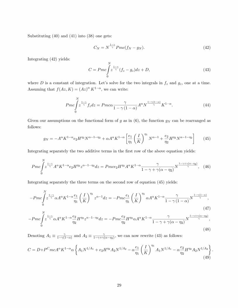
Substituting (40) and (41) into (38) one gets:

CN = N1� Pmc(fN � gN ): (42)

Integrating (42) yields:

C = Pmc

NZ0

z1� (fz � gz)dz +D; (43)

where D is a constant of integration. Let�s solve for the two integrals in fz and gz, one at a time.

Assuming that f(Az;K) = (Az)�K1��, we can write:

Pmc

NZ0

z1� fzdz = Pmc�

1� (1� �)A�N

1� (1��) K1��: (44)

Given our assumptions on the functional form of g as in (6), the function gN can be rearranged as

follows:

gN = �A�K1��e2H�2N��1��2 + �A�K1��

�e1�1

�I

K

��1N��1 +

e2�2H�2N��1��2

�(45)

Integrating separately the two additive terms in the �rst row of the above equation yields:

Pmc

NZ0

z1� A�K1��e2H

�2z��1��2dz = Pmce2H�2A�K1��

1� + (�� �2)N

1� + (���2) ; (46)

Integrating separately the three terms on the second row of equation (45) yields:

�PmcNZ0

z1� �A�K1�� e1

�1

�I

K

��1z��1dz = �Pmce1

�1

�I

K

��1�A�K1��

1� (1� �)N1� (1��)

;

(47)

�PmcNZ0

z1� �A�K1�� e2

�2H�2z��1��2dz = �Pmce2

�2H�2�A�K1��

1� + (�� �2)N

1� + (���2) ;

(48)

Denoting A1 � 1� (1��) and A2 �

1� + (���2) , we can now rewrite (43) as follows:

C = D+PCmcA�K1���

�A1N

1=A1 + e2H�2A2N

1=A2 � �e1�1

�I

K

��1A1N

1=A1 � �e2�2H�2A2N

1=A2

�:

(49)

29

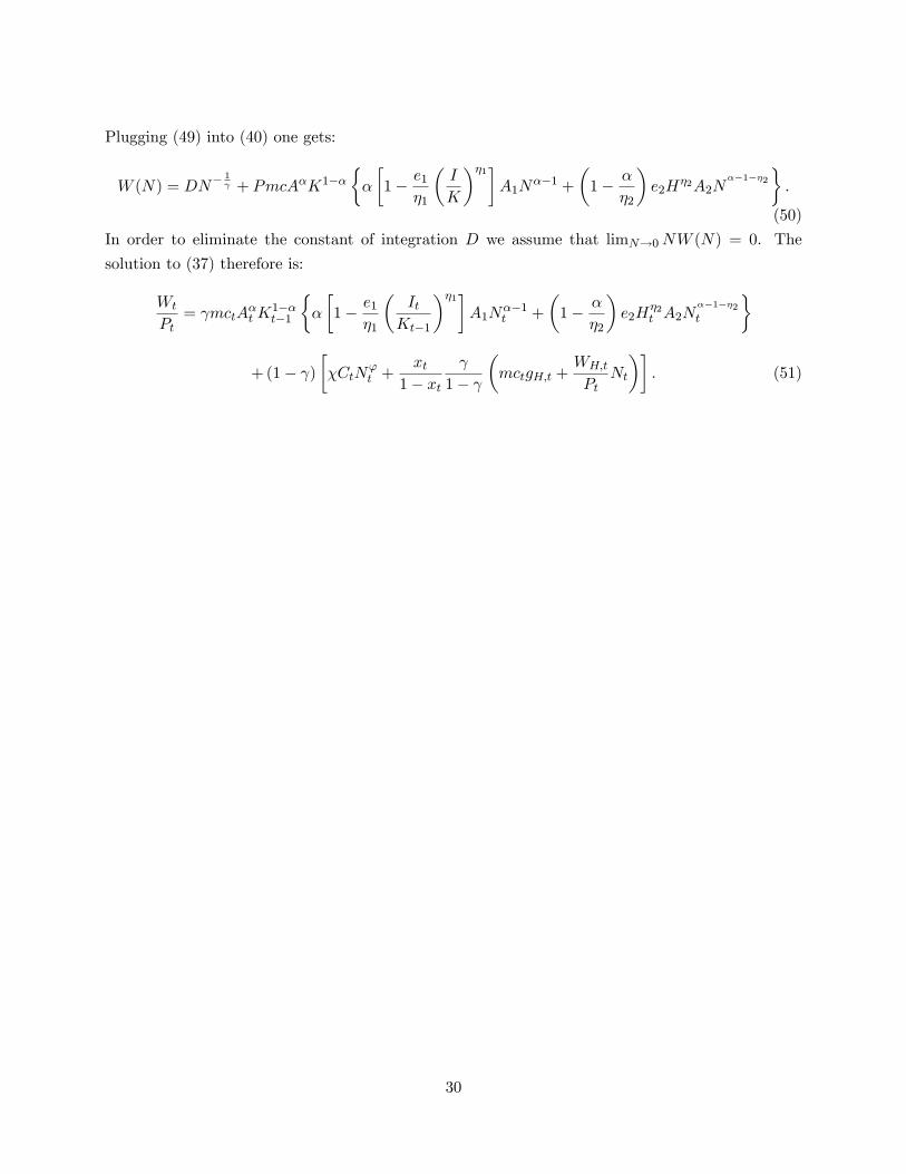
Plugging (49) into (40) one gets:

W (N) = DN� 1 + PmcA�K1��

��

�1� e1

�1

�I

K

��1�A1N

��1 +

�1� �

�2

�e2H

�2A2N��1��2

�:

(50)

In order to eliminate the constant of integration D we assume that limN!0NW (N) = 0. The

solution to (37) therefore is:

Wt

Pt= mctA

�t K

1��t�1

��

�1� e1

�1

�ItKt�1

��1�A1N

��1t +

�1� �

�2

�e2H

�2t A2N

��1��2t

�

+(1� )��CtN

't +

xt1� xt

1�

�mctgH;t +

WH;t

PtNt

��: (51)

30

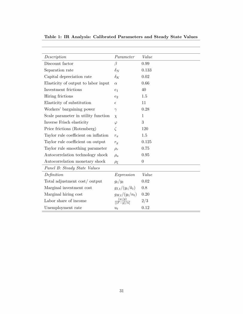
Table 1: IR Analysis: Calibrated Parameters and Steady State Values

Description Parameter Value

Discount factor � 0:99

Separation rate �N 0:133

Capital depreciation rate �K 0:02

Elasticity of output to labor input � 0:66

Investment frictions e1 40

Hiring frictions e2 1:5

Elasticity of substitution � 11

Workers�bargaining power 0:28

Scale parameter in utility function � 1

Inverse Frisch elasticity ' 3

Price frictions (Rotemberg) � 120

Taylor rule coe¢ cient on in�ation r� 1:5

Taylor rule coe¢ cient on output ry 0:125

Taylor rule smoothing parameter �r 0:75

Autocorrelation technology shock �a 0:95

Autocorrelation monetary shock �� 0

Panel B: Steady State Values

De�nition Expression Value

Total adjustment cost/ output gt=yt 0:02

Marginal investment cost gI;t=(yt=kt) 0:8

Marginal hiring cost gH;t=(yt=nt) 0:20

Labor share of income (w=p)[(F�g)=n] 2=3

Unemployment rate ut 0:12

31

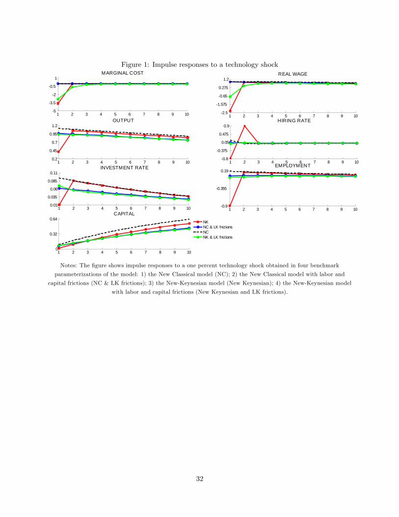
Figure 1: Impulse responses to a technology shock

1 2 3 4 5 6 7 8 9 10­5

­3.5

­2

­0.5

1MARGINAL COST

1 2 3 4 5 6 7 8 9 10­2.5

­1.575

­0.65

0.275

1.2REAL WAGE

1 2 3 4 5 6 7 8 9 100.2

0.45

0.7

0.95

1.2OUTPUT

1 2 3 4 5 6 7 8 9 10­0.8

­0.375

0.05

0.475

0.9HIRING RATE

1 2 3 4 5 6 7 8 9 100.01

0.035

0.06

0.085

0.11INVESTMENT RATE

1 2 3 4 5 6 7 8 9 10­0.9

­0.355

0.19EMPLOYMENT

1 2 3 4 5 6 7 8 9 100

0.32

0.64CAPITAL

NKNC & LK frictionsNCNK & LK frictions

Notes: The �gure shows impulse responses to a one percent technology shock obtained in four benchmark

parameterizations of the model: 1) the New Classical model (NC); 2) the New Classical model with labor and

capital frictions (NC & LK frictions); 3) the New-Keynesian model (New Keynesian); 4) the New-Keynesian model

with labor and capital frictions (New Keynesian and LK frictions).

32

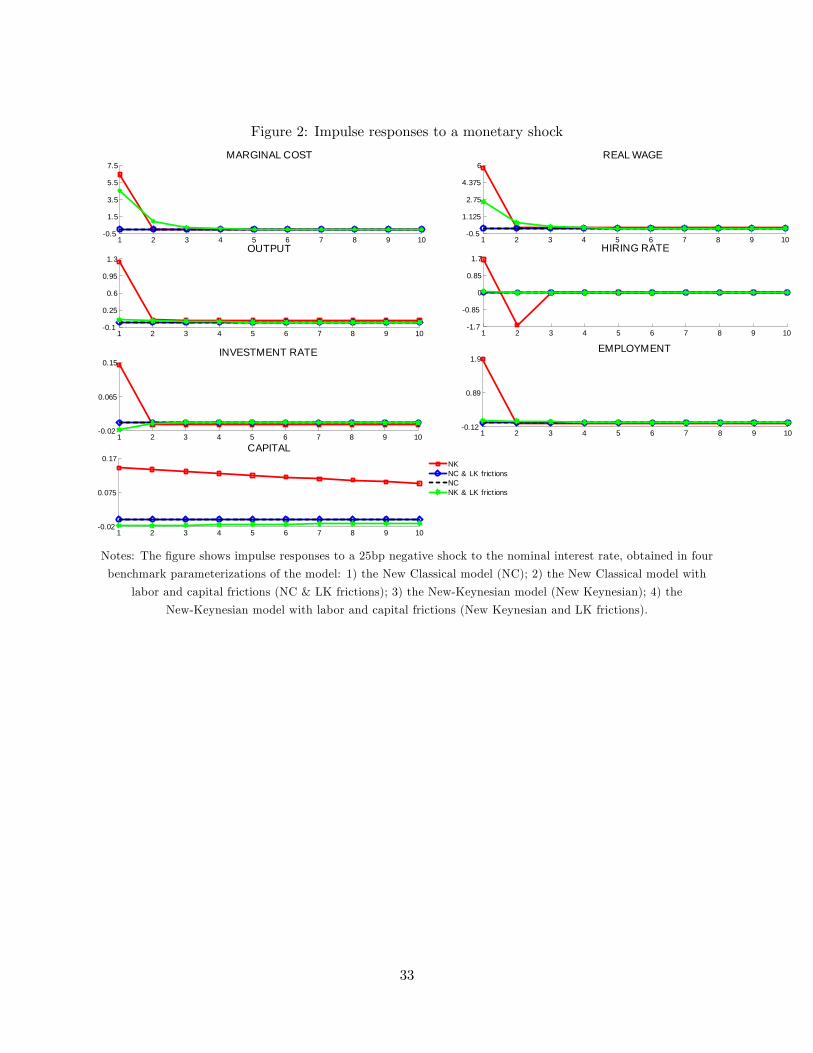
Figure 2: Impulse responses to a monetary shock

1 2 3 4 5 6 7 8 9 10­0.5

1.5

3.5

5.5

7.5MARGINAL COST

1 2 3 4 5 6 7 8 9 10­0.5

1.125

2.75

4.375

6REAL WAGE

1 2 3 4 5 6 7 8 9 10­0.1

0.25

0.6

0.95

1.3OUTPUT

1 2 3 4 5 6 7 8 9 10­1.7

­0.85

0

0.85

1.7HIRING RATE

1 2 3 4 5 6 7 8 9 10­0.02

0.065

0.15INVESTMENT RATE

1 2 3 4 5 6 7 8 9 10­0.12

0.89

1.9EMPLOYMENT

1 2 3 4 5 6 7 8 9 10­0.02

0.075

0.17CAPITAL

NKNC & LK frictionsNCNK & LK frictions

Notes: The �gure shows impulse responses to a 25bp negative shock to the nominal interest rate, obtained in four

benchmark parameterizations of the model: 1) the New Classical model (NC); 2) the New Classical model with

labor and capital frictions (NC & LK frictions); 3) the New-Keynesian model (New Keynesian); 4) the

New-Keynesian model with labor and capital frictions (New Keynesian and LK frictions).

33

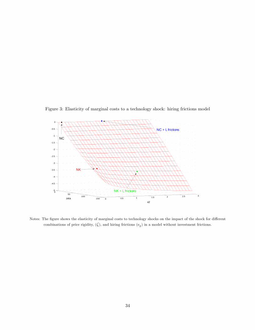
Figure 3: Elasticity of marginal costs to a technology shock: hiring frictions model

050

100150 0 0.5 1 1.5 2 2.5 3

­5

­4.5

­4

­3.5

­3

­2.5

­2

­1.5

­1

­0.5

0

zetae2

NC

NC + L frictions

NK

NK + L frictions

Notes: The �gure shows the elasticity of marginal costs to technology shocks on the impact of the shock for di¤erent

combinations of price rigidity, (�), and hiring frictions (e2) in a model without investment frictions.

34

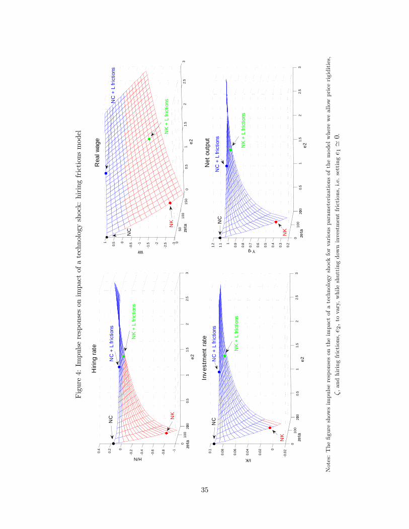
Figure4:Impulseresponsesonimpactofatechnologyshock:hiringfrictionsmodel

010

020

00

0.5

11.

52

2.5

3

­1

­0.8

­0.6

­0.4

­0.20

0.2

0.4

Hiri

ng r

ate

H/N

050

100

150

00.

51

1.5

22.

53

­3

­2.5­2

­1.5­1

­0.50

0.51

Rea

l wag

e

Wr

010

020

000.

51

1.5

22.

53

­0.0

20

0.02

0.04

0.06

0.080.

1In

ves

tmen

t ra

te

I/K

010

020

000.

51

1.5

22.

53

0.2

0.3

0.4

0.5

0.6

0.7

0.8

0.91

1.1

1.2

Net

 out

put

Y­g

e2e2

e2e2

zeta

zeta

zeta

zeta

NC

NC

 + L

 fric

tions

NK

NK

 + L

 fric

tions

NC

NK

NC

 + L

 fric

tions

NK

 + L

 fric

tions

NC

NC

 + L

 fric

tions

NK

 + L

 fric

tions

NK

NC

NC

 + L

 fric

tions

NK

NK

 + L

 fric

tions

Notes:The�gureshowsimpulseresponsesontheimpactofatechnologyshockforvariousparameterizationsofthemodelwhereweallowpricerigidities,

�,andhiringfrictions,e 2,tovary,whileshuttingdowninvestmentfrictions,i.e.settinge 1'0.

35

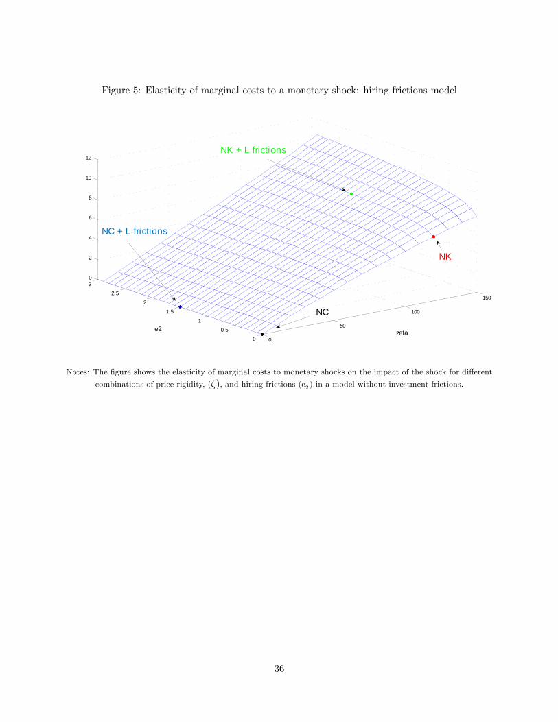
Figure 5: Elasticity of marginal costs to a monetary shock: hiring frictions model

0

50

100

150

0

0.5

1

1.5

2

2.5

30

2

4

6

8

10

12

zetae2

NC + L frictions

NK + L frictions

NC

NK

Notes: The �gure shows the elasticity of marginal costs to monetary shocks on the impact of the shock for di¤erent

combinations of price rigidity, (�), and hiring frictions (e2) in a model without investment frictions.

36

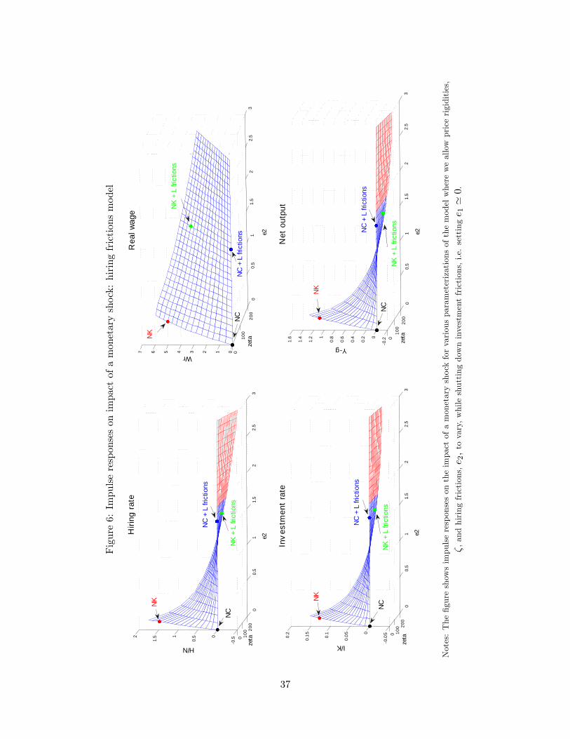
Figure6:Impulseresponsesonimpactofamonetaryshock:hiringfrictionsmodel

0 100

200

00

.51

1.5

22

.53

­0.50

0.51

1.52

Hiri

ng r

ate

e2

H/N

0

100

200

00

.51

1.5

22

.53

01234567

Rea

l wag

e

e2

Wr

0 100

200

00

.51

1.5

22

.53

­0.0

50

0.0

5

0.1

0.1

5

0.2

Inv

estm

ent 

rate

e2

I/K

01

002

000

0.5

11

.52

2.5

3

­0.20

0.2

0.4

0.6

0.81

1.2

1.4

1.6

Net

 out

put

e2

Y­gzeta ze

taze

ta

zeta

NC

NC

NC

NC

NK

NK

NK

NK

 + L

 fric

tions

NK

 + L

 fric

tions

NK

 + L

 fric

tions

NK

 + L

 fric

tions

NC

 + L

 fric

tions

NC

 + L

 fric

tions

NC

 + L

 fric

tions

NK

NC

 + L

 fric

tions

Notes:The�gureshowsimpulseresponsesontheimpactofamonetaryshockforvariousparameterizationsofthemodelwhereweallowpricerigidities,

�,andhiringfrictions,e 2,tovary,whileshuttingdowninvestmentfrictions,i.e.settinge 1'0.

37

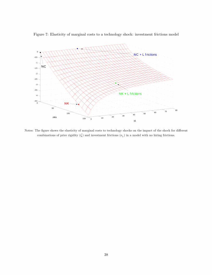
Figure 7: Elasticity of marginal costs to a technology shock: investment frictions model

0

50

100

150 0 10 20 30 40 5060 70

80

­4.5

­4

­3.5

­3

­2.5

­2

­1.5

­1

­0.5

0

e1

zeta

NC

NK

NK + L f rictions

NC + L f rictions

Notes: The �gure shows the elasticity of marginal costs to technology shocks on the impact of the shock for di¤erent

combinations of price rigidity (�) and investment frictions (e1) in a model with no hiring frictions.

38

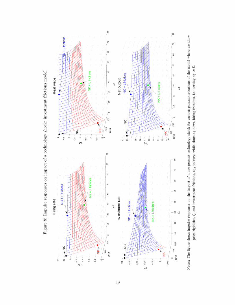
Figure8:Impulseresponsesonimpactofatechnologyshock:investmentfrictionsmodel

010

020

00

1020

3040

5060

7080

­1

­0.8

­0.6

­0.4

­0.20

0.2

0.4

Hiri

ng r

ate

e1

H/N

010

020

00

1020

3040

5060

7080

­3

­2.5­2

­1.5­1

­0.50

0.51

Rea

l wag

e

e1

Wr

010

020

0010

2030

4050

6070

80

­0.0

20

0.02

0.04

0.06

0.080.

1In

ves

tmen

t ra

te

e1

I/K

010

020

00

1020

3040

5060

7080

0.2

0.3

0.4

0.5

0.6

0.7

0.8

0.91

1.1

1.2

Net

 out

put

e1

Y­g

zeta

NC

NC

NK

NK

NK

 + L

 fric

tions

NK

 + L

 fric

tions

NK

 + L

 fric

tions

zeta

zeta

zeta

NC

NC

 + L

 fric

tions

NC

 + L

 fric

tions

NC

 + L

 fric

tions

NK

NK

 + L

 fric

tions

NK

NC

NC

 + L

 fric

tions

Notes:The�gureshowsimpulseresponsesontheimpactofaonepercenttechnologyshockforvariousparameterizationsofthemodelwhereweallow

pricerigidities,�,andinvestmentfrictions,e 1,tovary,whileshuttingdownhiringfrictions,i.e.settinge 2'0.

39

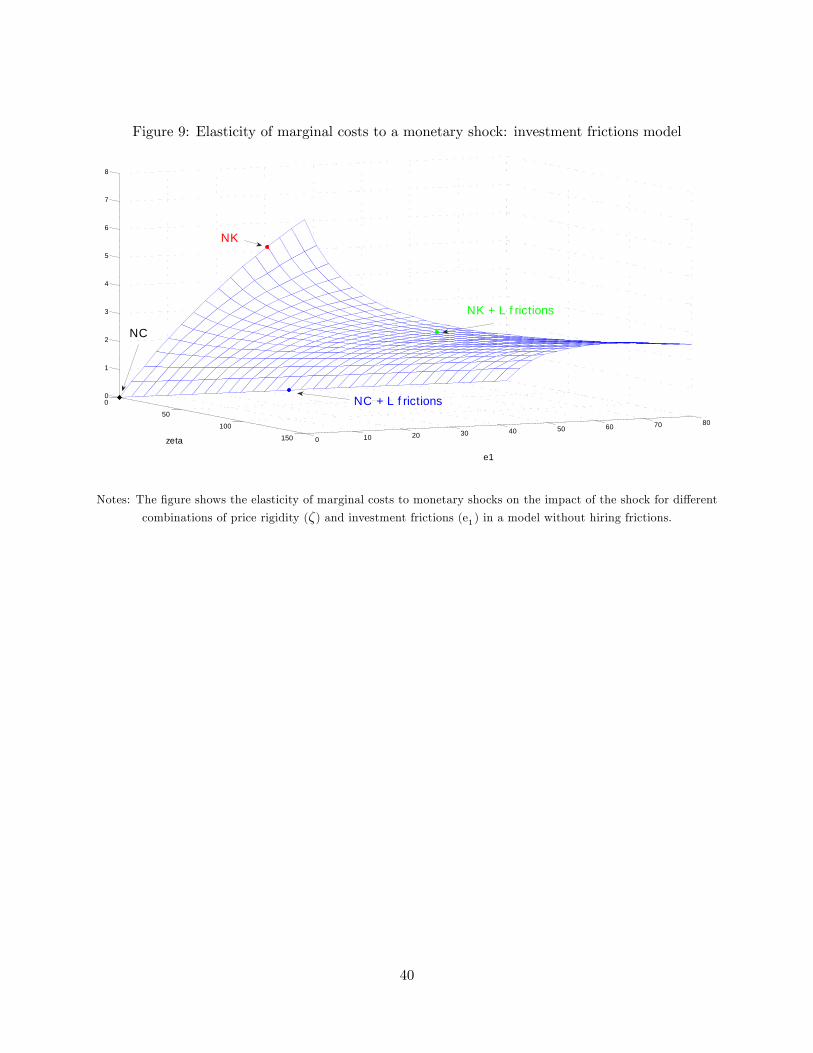
Figure 9: Elasticity of marginal costs to a monetary shock: investment frictions model

0

50

100

150 0 10 20 30 40 50 60 70 80

0

1

2

3

4

5

6

7

8

e1

zeta

NC

NK

NK + L f rictions

NC + L f rictions

Notes: The �gure shows the elasticity of marginal costs to monetary shocks on the impact of the shock for di¤erent

combinations of price rigidity (�) and investment frictions (e1) in a model without hiring frictions.

40

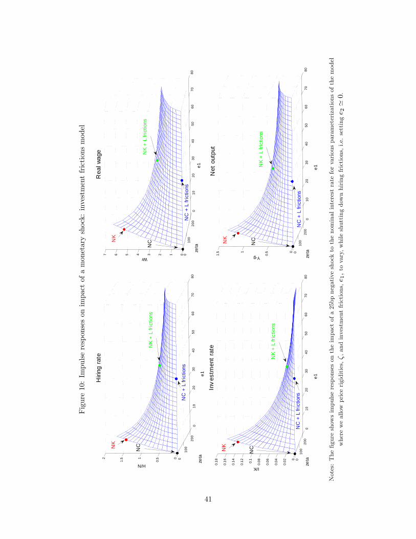
Figure10:Impulseresponsesonimpactofamonetaryshock:investmentfrictionsmodel

0

100

200

010

2030

4050

6070

80

0

0.51

1.52

Hiri

ng r

ate

e1

H/N

010

020

00

1020

3040

5060

7080

01234567

Rea

l wag

e

Wr

010

020

00

1020

3040

5060

7080

0

0.02

0.04

0.06

0.080.

1

0.12

0.14

0.16

0.18

Inv

estm

ent 

rate

e1

I/K

010

020

00

1020

3040

5060

7080

0

0.51

1.5

Net

 out

put

e1

Y­g

zeta

zeta

zeta

zeta

e1

NC NC

NCNC

NK

NK

NK

NK

NK

 + L

 fric

tions

NK

 + L

 fric

tions

NK

 + L

 fric

tions

NK

 + L

 fric

tions

NC

 + L

 fric

tions

NC

 + L

 fric

tions

NC

 + L

 fric

tions

NC

 + L

 fric

tions

Notes:The�gureshowsimpulseresponsesontheimpactofa25bpnegativeshocktothenominalinterestrateforvariousparameterizationsofthemodel

whereweallowpricerigidities,�,andinvestmentfrictions,e 1,tovary,whileshuttingdownhiringfrictions,i.e.settinge 2'0.

41