consequencesofburstystar formationon galaxy observablesat ... · consequencesofburstystar...

arX

iv:1

408.

5788

v2 [

astr

o-ph

.GA

] 1

5 M

ay 2

015

Mon. Not. R. Astron. Soc. 000, 1–12 (2013) Printed 12 November 2018 (MN LATEX style file v2.2)

Consequences of bursty star formation on galaxy

observables at high redshifts

Alberto Domınguez1,2⋆, Brian Siana1, Alyson M. Brooks3, Charlotte R. Christensen4

Gustavo Bruzual5, Daniel P. Stark6 and Anahita Alavi11Department of Physics & Astronomy, University of California Riverside, Riverside, CA 92521, USA2Department of Physics & Astronomy, Clemson University, Clemson, SC 29634, USA3Department of Physics & Astronomy, Rutgers, The State University of New Jersey, Piscataway, NJ 08854, USA4Grinnell College Physics Department, Noyce Science Center, Grinnell, IA 50112, USA5Centro de Radioastronomıa y Astrofısica, UNAM, Campus Morelia, Michoacan, 58089, Mexico6Steward Observatory, University of Arizona, 933 N Cherry Ave, Tucson, AZ 85721, USA

12 November 2018

ABSTRACT

The star formation histories (SFHs) of dwarf galaxies are thought to be bursty, withlarge – order of magnitude – changes in the star formation rate on timescales similar toO-star lifetimes. As a result, the standard interpretations of many galaxy observables(which assume a slowly varying SFH) are often incorrect. Here, we use the SFHsfrom hydro-dynamical simulations to investigate the effects of bursty SFHs on sampleselection and interpretation of observables and make predictions to confirm such SFHsin future surveys. First, because dwarf galaxies’ star formation rates change rapidly,the mass-to-light ratio is also changing rapidly in both the ionizing continuum and,to a lesser extent, the non-ionizing UV continuum. Therefore, flux limited surveys arehighly biased toward selecting galaxies in the burst phase and very deep observationsare required to detect all dwarf galaxies at a given stellar mass. Second, we show thata log10[νLν(1500A)/LHα] > 2.5 implies a very recent quenching of star formation andcan be used as evidence of stellar feedback regulating star formation. Third, we showthat the ionizing continuum can be significantly higher than when assuming a constantSFH, which can affect the interpretation of nebular emission line equivalent widthsand direct ionizing continuum detections. Finally, we show that a star formation rateestimate based on continuum measurements only (and not on nebular tracers such asthe hydrogen Balmer lines) will not trace the rapid changes in star formation and willgive the false impression of a star-forming main sequence with low dispersion.

Key words: galaxies: evolution – galaxies: high-redshift – galaxies: starburst

1 INTRODUCTION

One of the most important results derived from deep galaxysurveys is that star formation in the more massive galax-ies (galaxies with stellar masses larger than approximately109 M⊙) is regulated by gradual processes such as gas ex-haustion (e.g., Noeske et al. 2007a). This fact implies thatthe star formation history (SFH) of these galaxies can bedescribed by slowly varying functions of time (on timescaleslarger than approximately 100 Myr). However, stochasticprocesses are expected to dominate in dwarf galaxies (galax-ies with stellar masses lower than approximately 109 M⊙).Specifically, the star formation in dwarf galaxies occurs inonly a small number of regions and in a small volume. In

⋆ E-mail: [email protected]

such systems, feedback from supernovae can heat and ex-pel gas from a volume comparable to the entire volumeof the cold gas region, resulting in a temporary quench-ing of star formation. Therefore, the SFHs of dwarf galax-ies are characterized by frequent bursts of star formationand subsequent quenching (on timescales of the order of afew Myr; e.g., Shen et al. 2013; Hopkins et al. 2013). Thisburstiness may be caused mainly by supernovae feedback(e.g., Governato et al. 2012; Teyssier et al. 2013). BurstySFHs complicate our interpretation of observable properties,and oversimplification of these SFHs may lead to significantbiases in determinations of fundamental galaxy properties(e.g., Boquien, Buat & Perret 2014).

Recent studies are showing that low mass galaxiesat high redshift are contributing significantly to the to-tal star formation rate density (Alavi et al. 2014). Under-

c© 2013 RAS

http://arxiv.org/abs/1408.5788v2

2 A. Domınguez et al.

standing these low mass galaxies, especially at z ∼ 2–3when the star formation rate (SFR) of the Universe peaked(Reddy & Steidel 2009), is essential for explaining a numberof phenomena in the early Universe.

First, it is thought that dwarf galaxies reionized theintergalactic medium at z > 7 and provided a signifi-cant fraction of the ionizing background at 2 < z <7 (Haardt & Madau 2012; Becker & Bolton 2013). Manyinvestigations of escaping Lyman continuum from galax-ies are necessarily conducted at redshifts of 2 < z <3.5 (Vanzella et al. 2010; Nestor et al. 2013; Mostardi et al.2013), as the IGM becomes more opaque at higher red-shift (Prochaska, Worseck & O’Meara 2009). In these stud-ies, one typically assumes an intrinsic Lyman continuumflux based on the non-ionizing UV flux at approximately1500 A (Siana et al. 2007). However, this conversion usuallyassumes constant star formation for a long duration (longerthan 100 Myr). The bursty SFHs of dwarf galaxies will sig-nificantly affect the level of Lyman continuum flux, the se-lection of the galaxies, and our interpretation of the globalescape fraction of Lyman continuum photons. Furthermore,the bursty star formation also has important implicationsfor interpreting the byproducts of the Lyman continuum(i.e., nebular emission lines) in dwarf galaxies.

Second, among more massive galaxies, there is atight correlation between star formation and stellarmass. This correlation, called the star-forming mainsequence, may exist from the local Universe up toz ∼ 6 (e.g., Brinchmann et al. 2004; Noeske et al. 2007b;Pannella et al. 2009; Whitaker et al. 2012; Speagle et al.2014). These observations lead to the interpretation, men-tioned above, that star formation in these galaxies ispredominantly regulated by gradual processes. Whetherthis tight relation remains at lower masses is still un-clear, although very recently progress has been made byWhitaker et al. (2014) in measuring the average main se-quence in lower mass galaxies. Bursty star formation shouldincrease the dispersion in this relation. Unfortunately, thestar formation indicators that we typically use, namely ul-traviolet (UV) and infrared (IR) fluxes, vary on much largertime scales than the star formation in dwarf galaxies. It istherefore possible that we are not able to detect an increasedscatter in the SFR at low mass with these traditional indi-cators.

In this paper, we analyze how bursty SFHs produced byhydro-dynamical simulations affect our current knowledgeof the two issues stated above: the ionizing photon produc-tion and its subsequent effect on observables (e.g., nebularline strengths, searches for escaping Lyman continuum), andthe appearance of a tight star-forming main sequence. Themethodology is based on using a stellar population synthe-sis code to model the spectral energy distributions (SEDs)of these bursty galaxies, which cover the stellar mass rangefrom 107 M⊙ to 1010 M⊙ at z ∼ 2. Physical galaxy proper-ties such as stellar masses and star-formation rates are alsoderived by using SED fitting, which are compared with theirknown values from the model galaxies (e.g., Pacifici et al.2012).

This paper is organized as follows. In §2, we briefly de-scribe our hydro-dynamical simulations. Then, §3 gives de-tails on the extraction of the galaxy SEDs from the results ofthe simulations. Later, §4 shows the results from our analy-

sis in terms of the ionizing photon production and discussesthem. Then, §5 analyzes the star-forming main sequence. In§6, we compare physical galaxy properties from the modelSEDs and the SED fitting. Finally, we summarize in §7 themain conclusions of our analysis. Throughout the paper,we use the same cosmology assumed by the simulations,this is, a ΛCDM cosmology with H0 = 73 km s−1 Mpc−1,Ωm = 0.24, and ΩΛ = 0.76 (according to data from thethird release of the Wilkinson Microwave Anisotropy Probe,WMAP 3, Spergel et al. 2007).

2 GALAXY SIMULATIONS

The bursty in-situ SFHs used in our analysis, defined as thestar formation that occurs within the most massive progeni-tor of the main halo, are extracted from the hydro-dynamicalsimulations that are described in this section.

2.1 Details of the simulations

The high-resolution simulations used in this work were runusing the volume re-normalization technique (or zoom-in

technique) with the N-body plus smoothed-particle hydro-dynamics code GASOLINE (Wadsley et al. 2004). The galax-ies were selected to span a range of merger histories. All11 of the galaxies in this work have been published anddiscussed more extensively in previous papers. Importantlyfor this work, earlier papers using these simulated galax-ies have shown that they have realistic rotation curves(Christensen et al. 2014), that they match the z = 0 stellarmass to halo mass relation derived from abundance match-ing techniques (Munshi et al. 2013), and that the bursty starformation history in the seven lowest mass galaxies leads tothe creation of dark matter cores in their central density pro-files (Governato et al. 2012). These simulations also matchthe observed mass–metallicity relation (Brooks et al. 2007),the sizes of galaxy disks (Brooks et al. 2011), and result in arealistic population of satellites in Milky Way-mass galaxies(Zolotov et al. 2012; Brooks & Zolotov 2014). These simu-lated galaxies are among the highest resolution achieved incosmological simulations to date. The high resolution allowsus to resolve the high density gas clouds where stars form.With this scheme, we have successfully matched a largerange of observed galaxy properties, as mentioned above.An extensive discussion of the star formation and feedbackscheme in these simulations is found in Christensen et al.(2012). Below, we summarize the salient information aboutthe simulations.

The spline force softening in these simulations rangesfrom 65 pc (h2003) to 87 pc (h516 and h799) to 174 pc(all others). High resolution dark matter particles havemasses of 6661 M⊙ (1.3×105 M⊙), while gas particles startwith 1407 M⊙ (2.7×104 M⊙) for the lowest (largest) massgalaxies. Star particles are born with 30% of the massof their parent gas particle and lose mass through super-nova (both Ia and II) and stellar winds. Each of thesegalaxies has between one to five million dark matter par-ticles within the virial radius at z = 0. The simulationsnot only include metal line cooling and metal diffusion(Shen et al. 2010), but a prescription for the formation

c© 2013 RAS, MNRAS 000, 1–12

Consequences of bursty star formation 3

Simulation log10(M∗/M⊙)

z = 2 z = 0

h2003.grp1 6.97 7.05h799.grp1 7.07 7.64h516.grp1 7.70 8.05

h986.grp3 8.29 –h603.grp1 8.35 9.45h986.grp2 8.41 –h986.grp1 8.51 9.29h239.grp1 9.09 10.25h285.grp1 9.33 10.29h258.grp1 9.43 10.22h277.grp1 9.94 10.33

Table 1. The first column lists the simulation name. The secondand third columns show the stellar masses at z = 2 and z = 0(respectively; see text for details) from the in-situ SFHs outputby the GALAXEV code. The galaxies are sorted increasingly fromtop to bottom by their stellar mass at z = 2. The h986.grp2 andh986.grp3 merge with the most massive progenitor h986.grp1 byz = 0.

(both gas-phase and on dust grains) and destruction (pri-marily photo-dissociation by Lyman-Werner radiation fromnearby stellar populations) of H2 (Christensen et al. 2012).Star formation is tied directly to the presence of H2, asobserved (Leroy et al. 2008; Bigiel et al. 2008; Blanc et al.2009; Bigiel et al. 2010; Schruba et al. 2011). These simula-tions also include a uniform UV background that turns onat z = 9, mimicking cosmic reionization following a modifiedversion of Haardt & Madau (2001).

Critically for this work, the force resolution of theseruns (65–174 pc) allows high density regions where starsform to be resolved (ρ & 100 amu/cm3, comparable to theaverage density in giant molecular clouds). Star formation inthe simulations is done in 1 Myr increments. That is, every1 Myr we identify the gas that is cold and dense enough toform stars. For all gas particles that meet this criterion, thereis a 10%×fH2 chance (where fH2 is the molecular fraction ofthat gas particle) that they will spawn a star particle. Thehigh resolutions allow for a physically motivated stellar andsupernova feedback scheme that injects energy locally backinto the interstellar medium (ISM, following Stinson et al.2006) rather than the adoption of an analytic prescriptionto model feedback globally. This local injection of energycan heat the surrounding gas such that star formation iscompletely shut down for a brief period (Stinson et al. 2007).In low mass dwarfs, this leads to a bursty SFH.

We follow each galaxy back to high z, identifying ateach output timestep the halo progenitor that containsmost of the stellar mass at lower z. We identify halos atall steps using the Amiga Halo Finder (Gill et al. 2004;Knollmann & Knebe 2009). Two of the halos (h986.grp2 andh986.grp3) merge with h986.grp1 at z < 1, and no longerexist as independent galaxies at z = 0.

There are other authors who simulate galaxies us-ing different ISM/feedback recipes but still obtain burstySFHs similar to ours (Shen et al. 2013; Hopkins et al. 2013;Ceverino et al. 2014; Trujillo-Gomez et al. 2014). Relevantto this paper is the fact that, as galaxy stellar mass de-creases, the dispersion in star formation rate increases, es-

0.0

0.1

0.2

0.3

SFR[M

⊙yr

−1 ]

h2003.grp1 In-situEx-situ

0

2

4

SFR[M

⊙yr

−1 ]

h986.grp1

1 2 3 4 5Age of the Universe [Gyr]

0

10

20

30

40

50

SFR[M

⊙yr

−1 ]

h277.grp1

Figure 1. The star formation history of three of our simu-lated galaxies. Galaxies are shown, from top to bottom, in or-der of increasing stellar mass at z = 2. These stellar masses arelog10(M∗/M⊙) = 6.97, 8.51, and 9.94. The blue line is the in-situstar formation, whereas the red line shows the ex-situ star forma-tion that becomes part of the galaxy by z ∼ 2. The shaded regionshows the time range where the galaxy SEDs are extracted, whenthe Universe is between 2.5 and 3.5 Gyr old. Given our cosmol-ogy, these ages correspond to z = 2.74 and z = 1.97, respectively.The lower mass galaxies have more dramatic changes in SF onshort timescales, whereas the more massive galaxies have smaller

fractional variations, and on longer timescales

pecially on short time scales (< 100 Myr). We have calcu-lated the dispersion of SFRs for our simulated galaxies ondifferent time scales and find that the trend is similar to thevalues shown in Figure 12 of Hopkins et al. (2013). There-fore, the conclusions in our paper should broadly be true inother simulations as well.

2.2 Simulated star formation rate histories

Figure 1 shows the in-situ SFH of three of our 11 simulatedgalaxies. The SFHs of the lower mass galaxies are character-ized by complicated functions of time featuring short burstsof star formation. These bursts can reach an order of mag-nitude larger star formation rate than a rather quiescentstate in timescales of a few Myr or even less. Figure 1 alsoshows the ex-situ SFHs of the stars that are in the galaxiesat z ∼ 2. These are stars formed outside the main halo thatthrough mergers become part of the main galaxy by z ∼ 2.We stress that, as seen in Figure 1, the ex-situ contribution

c© 2013 RAS, MNRAS 000, 1–12


2.4 2.6 2.8 3.0 3.2 3.4 3.6Age of the Universe [Gyr]

0.5

1.0

1.5

2.0

2.5

3.0

3.5

log 1

0[L

ν(1500A

)/Lν(900A)]

h2003.grp1 h986.grp1 h277.grp1

Figure 2. The ratio between the continuum luminositieslog10[Lν(1500A)/Lν(900A)] as a function of age for three galax-ies of significantly different stellar mass. These galaxies are ourlowest mass galaxy h2003.grp1 (log10(M∗/M⊙) = 6.97), theintermediate mass galaxy h986.grp1 (log10(M∗/M⊙) = 8.51),and our largest mass galaxy h277.grp1 (log10(M∗/M⊙) = 9.94).The horizontal line marks the commonly assumed ratio oflog10[Lν(1500A)/Lν(900A)] = 0.84 (Siana et al. 2007). The re-peated quenching of star formation in low mass galaxies causesthe 900 A continuum luminosity to drop dramatically, resultingin large variations in the ratio.

is rather low compared to the in-situ star formation, partic-ularly in the lower mass galaxies that are the main targets ofthis study. Observational results from other authors such asBehroozi, Wechsler, & Conroy (2013) also suggest that thevast majority of all stars in low mass halos (by z ∼ 2) areformed in situ.

3 MODELING OF THE GALAXY SPECTRAL

ENERGY DISTRIBUTIONS

We use the stellar population synthesis code GALAXEV byBruzual & Charlot (2003, hereafter BC03) to determine thegalaxy SEDs and stellar masses from the simulated SFHs.We note that BC03 accurately traces the mass loss fromsupernovae. The BC03 stellar masses of our galaxies are re-ported in Table 1 for z = 2 and z = 0. These galaxies spanthe mass range from roughly 107–1010 M⊙ at z ∼ 2. Ourmodel SEDs are extracted at times when the Universe isfrom 2.5 Gyr to 3.5 Gyr old in steps of 5 Myr (a total of 201SEDs for each simulated SFH). These ages correspond toredshifts from z = 2.74 to z = 1.97 according to the cosmol-ogy of the simulations. Though we only output the SEDs at5 Myr intervals, it is important to note that we are usingSFHs with 1 Myr resolution. This is necessary for capturingstar formation changes on short time scales. The initial massfunction (IMF) is assumed to be given by Chabrier (2003)and the metallicity is fixed to Z = 0.2Z⊙, where Z⊙ is so-lar metallicity. This metallicity is roughly consistent withthe sub-solar metallicities measured in log10(M∗/M⊙) < 8at z ∼ 2 (Belli et al. 2013; Henry et al. 2013; Sanders et al.2014). No dust extinction is included. We neglect secondaryeffects of metallicity and dust to isolate the effects of burstystar formation on observable quantities.

From the model SEDs, we derive the UV luminosity

0.5 1.0 1.5 2.0 2.5 3.0 3.5log10 [Lν(1500A)/Lν(900A)]

0.05

0.10

0.15

0.20

0.25

0.30

#

M∗ > 109M⊙

108M⊙ ≤ M∗ ≤ 109M⊙

M∗ < 108M⊙

Figure 3. The normalized Lν(1500A)/Lν (900A) distributionsin three stellar mass bins. The vertical line marks the com-monly assumed ratio of log10[Lν(1500A)/Lν(900A)] = 0.84(Siana et al. 2007). Low mass galaxies have a larger distributionof Lν(1500A)/Lν (900A), with larger ratios shortly after star for-mation quenching and lower ratios immediately after a new burstof star formation.

in the continuum at two different wavelengths: the ionizingcontinuum at 900 A (also known as Lyman continuum, orLyC) and the non-ionizing continuum at 1500 A, where mostobservational studies easily detect high redshift galaxies.

The BC03 code outputs the number of ionizing photonsper second (N), which is used to estimate the Hβ emission-line luminosity (LHβ, in erg/s) as,

LHβ = 4.757 × 10−13N (1)

(see Krueger et al. 1995). This luminosity is necessary asa reference from which to derive other emission-line lumi-nosities. In our case, we consider Lyα and Hα, whose ratiosare LLyα/LHβ = 22.20 and LHα/LHβ = 2.87 (case B re-combination; Osterbrock & Ferland 2006). We assume thatall of the ionizing photons are absorbed by hydrogen in theISM of galaxies - that is, that the LyC escape fraction isnear zero. Although this choice may not be realistic for asubset of galaxies (e.g., Nestor et al. 2013; Mostardi et al.2013), only very large escape fractions (i.e., larger than ap-proximately 0.5) would significantly affect our results. Therest-frame Lyα and Hα equivalent widths (EWs) are calcu-lated from the model SEDs as the ratio between the lumi-nosity of the line and the continuum luminosity per unit ofwavelength at the central wavelength of the line. We do notapply any correction to account for stellar absorption in Hα.However, this choice will not substantially affect our resultssince Hα in absorption is typically small in young galaxies(e.g., Domınguez et al. 2013).

As we mentioned in §2, a small fraction of the stel-lar mass is formed ex-situ and becomes part of the galaxythrough mergers. Importantly for the subsequent analysis,the stellar mass produced ex-situ will not contribute to theLyC or UV photon emission since the star formation oc-curred long enough before coalescence.

c© 2013 RAS, MNRAS 000, 1–12


Stellar Mass Range [M⊙]

Standard deviation 6 108 108 − 109 > 109

log10 [Lν(1500A)/Lν(900A)] 0.74 0.23 0.09log10 (Lyα EW/A) 0.53 0.18 0.07log10 (Hα EW/A) 0.97 0.39 0.20log10 (SFR/M⊙ yr−1) >0.65 >0.47 0.26log10 [Lν(900A)/erg s−1 Hz−1] 1.03 0.45 0.22log10 (LHα/erg s−1) 1.03 0.45 0.22log10 [Lν(1500A)/erg s−1 Hz−1] 0.43 0.28 0.16log10 [Lν(5500A)/erg s−1 Hz−1] 0.15 0.11 0.06log10 [Lν(1.2µm)/erg s−1 Hz−1] 0.10 0.08 0.05

Table 2. The standard deviation of the quantities listed in col-umn 1 in three different stellar mass bins after removing the stellarmass trend. We are reporting only lower limits for the two lowerbins of the SFR because the values for SFR = 0 are not includedin the standard deviation calculation.

4 STUDY OF THE IONIZING PHOTON

PRODUCTION

The UV and Hα luminosities are directly related to starformation. The former, Lν(1500A) or LUV , is dominatedby light coming from young and massive O and B stars(& 3 M⊙). This indicator is sensitive to the recent SFR giventhe lifetime of the massive stars that produce it (. 100 Myr).The latter, LHα, is produced by ionizing radiation com-ing from nebular regions heated by extremely massive stars(& 20 M⊙). This indicator is sensitive to the instantaneousSFR since it is dominated by stars with very short life-time (. 5 Myr). According to BC03 models, after an in-stantaneous burst of star formation, it takes only 5 Myrfor Lν(900A) to decrease an order of magnitude, whereas ittakes 30 Myr for Lν(1500A). Results of our analysis in termsof the production of ionizing radiation and nebular emissionlines are discussed in this section.

4.1 Ionizing photon production

The SFRs of dwarf galaxies are expected to change on time-scales similar to lifetimes of the ionizing O-stars. Therefore,we might expect wide variations in the ionizing photon pro-duction rate in these systems.

The ratio between the continuum luminositiesLν(1500A)/Lν(900A) is typically used to derive therelative escape fraction of ionizing photons and also to con-vert from observed UV luminosity functions to LyC photonproduction rates (e.g., Steidel et al. 2001; Siana et al. 2007,2010). This flux ratio is usually assumed as a constant ratioof approximately 7 (or 0.84 in log10). This value is reachedwhen the equilibrium state is produced under continuousstar formation when the number of stars producing LyC and1500 A flux is constant (or about 200 Myr after the burst).The log10[Lν(1500A)/Lν(900A)] is shown in Figure 2 as afunction of time for three different galaxies. We see thatthe scatter of log10[Lν(1500A)/Lν(900A)] is significantlylarger in the low mass galaxies, varying by nearly an orderof magnitude on short time scales but only around 0.1 dexfor the larger mass galaxies.

In Figure 3, we show the normalized distribution oflog10[Lν(1500A)/Lν(900A)] for three different stellar massbins that include all evolutionary stages. From the anal-

0.5 1.0 1.5 2.0 2.5 3.0 3.5log10 [Lν(1500A)/Lν(900A)]

0.5

1.0

1.5

2.0

2.5

log 1

0(Lyα

intEW/A

)

Lyαint EW > 60 A

Lyαint EW < 60 A

h2003.grp1h986.grp1h277.grp1

Figure 4. The intrinsic Lyα EW versus Lν(1500A)/Lν (900A)for three galaxies of significantly different stellar mass at dif-ferent evolutionary stages. These galaxies are our lowest massgalaxy h2003.grp1 (log10(M∗/M⊙) = 6.97), the intermediatemass galaxy h986.grp1 (log10(M∗/M⊙) = 8.51), and our largestmass galaxy h277.grp1 (log10(M∗/M⊙) = 9.94). The evolution-ary stages above the horizontal line are considered typical Lyαemitters. In general, non-Lyα emitter are significantly faint inthe LyC. Though many LyC searches of high redshift galaxies arenot targeting low mass galaxies with low Lyα EW, those galaxieslikely do not have strong Lyman continuum luminosities anyway,as the star formation may have recently been quenched. For in-stance, our galaxy of lowest mass is a Lyα emitter for 57% of thetime.

ysis of our simulations, it is clear that the assumption oflog10[Lν(1500A)/Lν(900A)] ∼ 0.84 is valid for the largermass galaxies but not for the lower mass galaxies due tosignificantly large scatter. The scatter is quantified as thestandard deviation of the distribution in three stellar massbins in Table 2.

This scatter in Lν(1500A)/Lν(900A) in low mass galax-ies will require particular care in interpreting studies of es-caping LyC. First, there are some galaxies, caught just whena burst begins, that have large LyC luminosities relative tothe non-ionizing 1500 A luminosities. This will make themeasier to detect in direct LyC searches. These same galaxieswill have very high intrinsic (unextinguished by dust) LyαEW (see Figure 4). Therefore, galaxies selected for high LyαEW (e.g., Nestor et al. 2011; Mostardi et al. 2013) will havea higher likelihood of LyC detection than galaxies with lowerLyα EW, even if the LyC escape fractions are similar. Sec-ond, low mass galaxies that have recently turned off theirstar formation will still be reasonably luminous at 1500 A,but will not be producing significant LyC photons. In Fig-ure 3, we can see that 38% of low mass (M∗ < 108 M⊙)galaxies have log10[Lν(1500A)/Lν(900A)] > 1.3 (or above20 in linear terms). These galaxies would often result innon-detections in direct LyC surveys, even if the LyC es-cape fractions of these galaxies were high. Ultimately, theburstiness of star formation as a function of mass will needto be better determined and incorporated into any analysisof LyC observations. We note that in larger mass galax-ies (M∗ > 109M⊙), it is reasonable to assume a constantLν(1500A)/Lν(900A) because the star formation does nottypically change much on short time scales.

Nestor et al. (2011, 2013) find a high ionizing emissiv-

c© 2013 RAS, MNRAS 000, 1–12


ity from Lyα emitters at z = 3.09, possibly explaining theentire ionizing background at that redshift. This findingis initially surprising because only a subset of UV-brightgalaxies (Lyα emitters) is enough to explain, at least, asignificant fraction of the ionizing background. However, itmay be possible that Lyα-emitting galaxies are the onlyones producing significantly strong LyC. Indeed, this isshown in Figure 4, where we plot Lyα EW as a functionof log10[Lν(1500A)/Lν(900A)]. The horizontal line shownin Figure 4 defines typical Lyα emitters as intrinsic LyαEW larger than 60 A if we assume a Lyα escape fractionof 50%. (Typically Lyα emitters are selected at Lyα EWlarger than 30 A and have Lyα escape fractions of 30–60%,Gronwall et al. 2007; Ouchi et al. 2008; Nilsson et al. 2009.)As we see in the figure, in general, galaxies that are not Lyαemitters are by definition faint in the LyC. We stress herethat all of these Lyα EW predictions are intrinsic measuresbefore scattering by Hi and absorption by dust. Of course,most of the more massive, dusty galaxies, will not be Lyαemitters. Therefore, galaxies selected as Lyα emitters maybe primarily composed of lower mass galaxies (with lowercolumns of neutral hydrogen and dust) in a burst phase. De-termining exactly when each galaxy will be a Lyα-emitterrequires more detailed dust modeling and ray tracing, whichis beyond the scope of this paper. Nonetheless, we stress thatlow mass galaxies may not produce significant LyC abouthalf of the time and selection on high Lyα EW will missthese galaxies. Thus, it may not be surprising that a largefraction of the known ionizing background at high redshiftis caused by low mass galaxies selected as Lyα-emitters.

A potential problem in our calculations is the fact thatLyα photons significantly scatter with neutral hydrogenwithin the galaxy before escaping. This effect may producea delay in the escape of the photons from the galaxy, whichcould smooth the Lyα luminosity time variation. However,given the size of a typical dwarf galaxy at z ∼ 2 (of theorder of a kpc) any delay due to a large number of scattersshould be significantly smaller than the 1 Myr resolution ofour simulations.

4.2 Nebular emission-line equivalent width

Recently, very young galaxies have been found at z > 1 byidentifying galaxies with large EW nebular emission lines(van der Wel et al. 2011; Atek et al. 2011; Atek et al. 2014;Stark et al. 2014). In particular, the Hα EW is a proxy ofthe specific star-formation rate of a galaxy (i.e., the star-formation per unit of stellar mass). The rest-frame intrinsicLyα and Hα EWs are plotted in Figure 5 as a functionof stellar mass. Both EWs have a similar behaviour. Theirscatter increases in the low mass galaxies as a consequenceof the burstiness of the SFHs.

Table 2 quantifies the dispersion of the Lyα and HαEWs distribution as the standard deviation in three stellarmass bins. We note that the dispersion of the Hα EW islarger than the dispersion of Lyα EW at all masses. Thereason is that when the LyC is high (during a burst of starformation), both Lyα and Hα emission-line luminosities in-crease by the same factor. However, the rest-UV continuumat 1216 A also increase strongly at the same time, whereasthe continuum near 6563 A does not change as much as the

−1

0

1

2

3

log 1

0(Lyα

intEW/A

)

h2003.grp1h799.grp1h516.grp1h986.grp3h603.grp1h986.grp2

h986.grp1h239.grp1h285.grp1h258.grp1h277.grp1

7.0 7.5 8.0 8.5 9.0 9.5 10.0log10 (M∗/M⊙)

−1

0

1

2

3

log 1

0(H

αEW/A

)

Figure 5. The intrinsic Lyα (upper panel) and Hα EW (lowerpanel) versus stellar mass for our sample of 11 galaxies. Eachgalaxy is represented by a different color. A circle is plotted every5 Myr from times of 2.5 to 3.5 Gyr, which makes it a total of201 data points for each galaxy. We note that the range of they-axis is the same for both panels. The simulations predict a largepopulation of low mass galaxies with Hα EW lower than 30 A.

rest-UV continuum. Therefore, the Hα EW change is moredramatic.

The equivalent widths increase immediately following anew burst of star formation, as the ionizing photon produc-tion rate reacts immediately, but the continuum flux takesa longer time to increase. Conversely, a few Myr after thestar formation turns off, the LyC disappears but the 1500 Aflux fades much more slowly. Thus, the EWs quickly go tozero in recently quenched systems. We note that the plottedLyα EWs are maximum values because it is expected thata significant fraction of Lyα photons will be absorbed bydust as it scatters through the interstellar and circumgalac-tic media.

Two of the most common star formation rate indicatorsat high redshift are the UV and Hα luminosities. However, asseen above, the ionizing continuum responsible for producingHα can change on very short time scales but the UV contin-uum takes longer to react. Therefore, we expect that the UVand Hα-derived SFRs may differ significantly depending onwhen the galaxy is observed (e.g., Glazebrook et al. 1999).Figure 6 shows the log10[νLν(1500A)/LHα] as a function ofstellar mass. The log10[νLν(1500A)/LHα] tends to a valueof 2.05 for the larger mass galaxies. This value correspondsto luminosities from a galaxy with constant SFR when theequilibrium in the number of O-stars to UV-emitting starsis reached. We can see in Figure 6 that dwarf galaxies withbursty SFHs are characterized by log10[νLν(1500A)/LHα] >2.5 shortly after star formation has been quenched. Both

c© 2013 RAS, MNRAS 000, 1–12


−4

−3

−2

−1

0

1

2

log 1

0(SFR/M

⊙yr

−1)

h2003.grp1, σ > 0.58

h799.grp1, σ > 0.48

h516.grp1, σ > 0.65

h986.grp3, σ > 0.47

h603.grp1, σ > 0.37

h986.grp2, σ > 0.46

h986.grp1, σ > 0.50

h239.grp1, σ = 0.30

h285.grp1, σ = 0.26

h258.grp1, σ = 0.18

h277.grp1, σ = 0.20

7.0 7.5 8.0 8.5 9.0 9.5 10.0log10 (M∗/M⊙)

23

24

25

26

27

28

29

30

log 1

0[L

ν(1500A

)/ergs−

1Hz−

1]

GOODS F435W Flux Limit @ z = 2

HUDF F435W Flux Limit @ z = 2

h2003.grp1, σ = 0.25

h799.grp1, σ = 0.19

h516.grp1, σ = 0.39

h986.grp3, σ = 0.24

h603.grp1, σ = 0.22

h986.grp2, σ = 0.24

h986.grp1, σ = 0.28

h239.grp1, σ = 0.22

h285.grp1, σ = 0.14

h258.grp1, σ = 0.08

h277.grp1, σ = 0.11

37

38

39

40

41

42

43

log 1

0(L

Hα/erg

s−1)

3DHST/WISP Flux limit @ z = 1.4

h2003.grp1, σ = 1.00

h799.grp1, σ = 0.50

h516.grp1, σ = 0.98

h986.grp3, σ = 0.42

h603.grp1, σ = 0.35

h986.grp2, σ = 0.50

h986.grp1, σ = 0.42

h239.grp1, σ = 0.30

h285.grp1, σ = 0.23

h258.grp1, σ = 0.12

h277.grp1, σ = 0.15

7.0 7.5 8.0 8.5 9.0 9.5 10.0log10 (M∗/M⊙)

23

24

25

26

27

28

29

30

log 1

0[L

ν(5500A

)/ergs−

1Hz−

1]

h2003.grp1, σ = 0.06

h799.grp1, σ = 0.05

h516.grp1, σ = 0.14

h986.grp3, σ = 0.08

h603.grp1, σ = 0.09

h986.grp2, σ = 0.06

h986.grp1, σ = 0.09

h239.grp1, σ = 0.07

h285.grp1, σ = 0.05

h258.grp1, σ = 0.02

h277.grp1, σ = 0.04

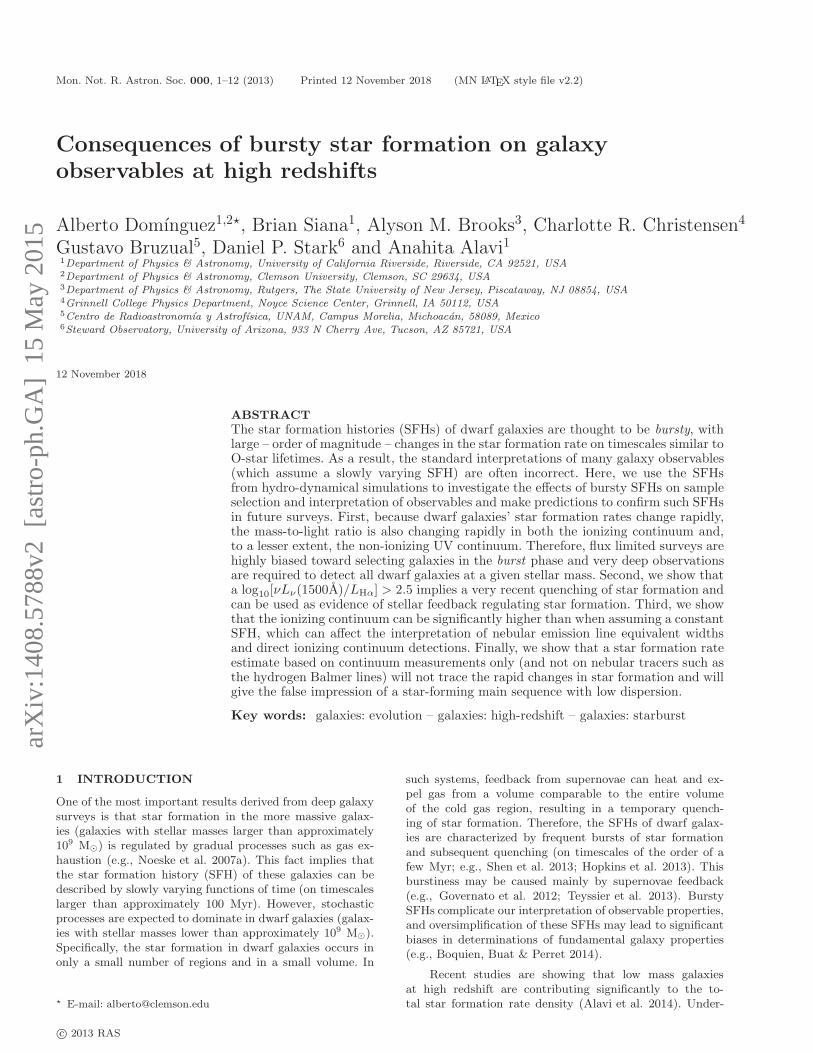
Figure 7. (Top left panel) The star formation rate from our simulations versus stellar mass. The best-fit straight line for the modelgalaxies (dotted line) is given by log10(SFR/M⊙ yr−1) = (1.05± 0.35)× log10(M∗/M⊙)− (9.25± 2.91). The scatter of the distributions(after removing the stellar mass trend) are given in the legends. Note that the evolutionary stages when the star formation rate of thegalaxy, given by the simulations, is zero cannot be plotted. The stars are average values calculated as explained in the text. Note thatall the panels show a range of 7 orders of magnitude in the y-axis. (Top right panel) The Hα luminosities versus stellar mass. The bestfit straight line for the model galaxies (dotted line) is given by log10(LHα/erg s−1) = (1.12 ± 0.35) × log10(M∗/M⊙) + (31.52 ± 2.90).The flux limit at z = 1.4 from the WISP/3DHST galaxy survey (Atek et al. 2010; Brammer et al. 2012) is shown with a dashed line.(Bottom left panel) The UV luminosities versus stellar mass. The best-fit straight line for the model galaxies (dotted line) is given bylog10(LUV /erg s−1 Hz−1) = (1.11± 0.35)× log10(M∗/M⊙) + (18.40± 2.90). The flux limits at z = 2 from the GOODS (B = 27.80, 5σ,0.2” radius, Giavalisco et al. 2004) and HUDF (B = 29.70, 5σ, 0.2” radius, Beckwith et al. 2006) galaxy surveys are shown with dashedlines. (Bottom right panel) The optical luminosities versus stellar mass. The best-fit straight line for the model galaxies (dotted line) isgiven by log10[L(5500 A)/erg s−1 Hz−1] = (1.03 ± 0.35) × log10(M∗/M⊙) + (19.25 ± 2.90). The slope of these relations are compatible

with 1. Because the Hα responds on short timescales, it accurately traces the rapidly varying SFR and has a similar scatter to thestar-forming main sequence. The dispersion in LUV also increases at lower mass, but not with the same amplitude of the SFR. Finally,the Lν(5500A) luminosity does not vary at all on the short time scales of the SFR variations.

Lν(1500A) and LHα are typically observed by deep galaxysurveys. Therefore, this figure provides a reliable test forbursty SFHs in star-forming galaxies based on large ratiosof the UV continuum at 1500 A and the Hα emission lumi-nosity. The effect of periodic bursty SFHs on the ratio of UVand Hα luminosity is studied in low redshift dwarf galax-ies by some authors such as Iglesias-Paramo et al. (2004),Boselli et al. (2009), Meurer et al. (2009) and Weisz et al.(2012). These authors use analytical models to explore theamplitude, duty cycle, and duration of bursts of star forma-tion by fitting the observed distribution of UV to Hα ra-tios. In our analysis, we take an alternative approach usingSFHs motivated by results from hydro-dynamical cosmolog-ical simulations.

4.3 Populating the IMF stochastically

At low SFRs, additional analysis uncertainties may arise dueto poor sampling of the high mass end of the IMF. Individ-ual bursts may also have different IMFs. Stochastic effectson the IMF have been studied by other authors such asFumagalli et al. (2011), Forero-Romero & Dijkstra (2013),and da Silva, Fumagalli, & Krumholz (2014) using the codeStochastically Lighting Up Galaxies by da Silva et al.(2012). According to Forero-Romero & Dijkstra (2013, seetheir Figure 1 and Figure 2) this effect becomes importantat star formation rates lower than 0.01 M⊙yr−1. From theexamples shown in our Figure 1, we note that the stellarmass involved in the bursts considered is sufficiently highthat individual bursts fairly sample the underlying IMF.

c© 2013 RAS, MNRAS 000, 1–12


7.0 7.5 8.0 8.5 9.0 9.5 10.0log10 (M∗/M⊙)

1.5

2.0

2.5

3.0

3.5

4.0

4.5

5.0

log 1

0[νLν(1500A

)/LHα]



Figure 6. The log10[νLν(1500A)/LHα] versus stellar mass forour galaxies. The dashed line shows that ratio at 2.05 for a con-stant SFH after a steady state is reached. The bursty SFHs ofthe numerical simulations predict that a population exists withlog10[νLν(1500A)/LHα] > 2.5 at log10(M∗/M⊙) < 8.5, a clearindicator of rapid quenching of star formation.

This implies that this stochasticity effect should not be toolarge in our sample. Though we expect this to be a minoreffect, it will result in a slight decrease in the distribution ofLyα and Hα EWs at the low mass end in Figure 5. However,all the main observational conclusions of this paper will notbe affected.

5 THE STAR-FORMING MAIN SEQUENCE

Typically, when evaluating trends in SFHs, the SFR is plot-ted as a function of stellar mass to show the star-formingmain sequence. Our theoretical work complements other ob-servational analyses of the main sequence. Here, we chooseto analyze directly the luminosities instead of the SFRs toavoid any uncertainties from their conversion.

In Figure 7, we plot the SFR versus stellar mass. Inaddition, three other observables are plotted in Figure 7,Hα luminosity, UV luminosity density, and optical luminos-ity density versus stellar mass. One can see that the largevariation in SFR in low mass galaxies is traced very well byHα as it reacts quickly to the changing SFR. The UV varia-tions are not as large as the SFR variations, and the opticalluminosity is essentially unaffected by the SFR variations.

Table 2 lists the standard deviation of these observablesin three mass bins. At large mass, the dispersion in SFR issmall, and both Hα and UV reasonably trace the SFR vari-ations (though Hα is certainly better). However, at lowermasses (M∗ < 109 M⊙), as the SFR variations increase, theUV dramatically under-predicts the SFR variation. There-fore, our results show that, for low mass galaxies, a tightcorrelation of LUV with stellar mass does not necessarilymean a smooth star formation history. Rather, it just meansthat a significant amount of the variance in star formationis on time scales shorter than it takes for the UV-emittingstars to react. As we study fainter galaxies, we must seek touse star formation indicators that trace shorter times scalessuch as Hα and other nebular emission lines.

We also emphasize that observationally a flux limitedsurvey will be strongly biased towards galaxies in the burst

phase. This is especially true when the selection is madeon emission lines because the luminosities change dramat-ically. For example, Figure 7 shows that the Hα selectionof recent HST WFC3/IR grism surveys (WISP, Atek et al.2010; 3DHST, Brammer et al. 2012) can detect galaxies atz ∼ 1.4 in a recent burst at stellar masses larger than108 M⊙, but will miss the vast majority of the galaxies ataround 108 M⊙. When the selection is made in the UV con-tinuum the bias will be less severe since the UV scatter islower but still significant. Figure 7 shows that the HUDFdepths (Beckwith et al. 2006) can detect galaxies currentlyin a burst at 107 M⊙ but the depths need to be an order ofmagnitude lower to detect all galaxies of that mass. Indeed,UV selection of dwarf galaxies at these redshifts (Alavi et al.2014) is still finding mostly galaxies which appear to be in astrong and recent burst of star formation (Stark et al. 2014).

Finally, we note that in Figure 7, we calculate theaverage of the SFR and each observable for each galaxyby adding all of the individual values at each time stepand dividing by the number of time steps (that is, to geta mean, rather than a geometric mean). The values areplotted with the large star symbols, and are analogous towhat observers would obtain when stacking large samplesof galaxies in bins of stellar mass. The slope of the aver-

age SFR versus M∗ relation is near one, consistent withthe slope measured by Whitaker et al. (2014) in galaxieswith 9.3 < log10(M∗/M⊙) < 10.2 at these high redshifts.However, other authors such as Henry et al. (2013) finda shallower slope of 0.31 ± 0.08 in galaxies with 8.2 <log10(M∗/M⊙) < 9.8. We believe this is a natural conse-quence of a bias toward galaxies in a burst phase when se-lecting via emission lines. As a result, the lowest mass galax-ies detected in that survey are those with the largest SFRs.Such a bias will naturally lead to perceiving a shallower mainsequence.

6 COMPARISON WITH PHYSICAL

PROPERTIES FROM SED FITTING

In this section, we explore how well SED fitting to broad-band photometry can determine the physical properties ofbursty galaxies. In particular, we examine the effects of theincorrect parameterization of the SFH on determining thegalaxies SFRs and stellar masses.

The code Fitting and Assessment of Synthetic Tem-plates (FAST, see the appendix in Kriek et al. 2009 for de-tails) is used to find the best fitting SED template froma grid of BC03 models. This fitting procedure is appliedto the model galaxies simulating the following photom-etry: the UV/optical channel (UVIS) of the Wide-fieldCamera 3 (WFC3) on board the Hubble Space Telescope(HST), the Advance Camera Survey (ACS)/WFC (F475W,F625W, F775W and F850LP) and the near-infrared (IR)with WFC3/IR (F125W and F160W). This is the same pho-tometry used by Alavi et al. (2014) and it spans the rest-UV to rest-optical across the Balmer/4000A break. Nebu-lar emission lines are not included in the photometry, norare they considered in the SED templates. Therefore, weare isolating the effects of the bursty SFHs independent ofcomplications due to emission line contributions to broad-band photometry. A signal-to-noise of 20 is assumed for each

c© 2013 RAS, MNRAS 000, 1–12


2.6 2.8 3.0 3.2 3.4Age of the Universe [Gyr]

−2.5

−2.0

−1.5

−1.0

−0.5

0.0

0.5

1.0

log 1

0(SFR/M

⊙yr

−1)

h986.grp1Simulated

Binned Simulated

SED fitting

Figure 8. The galaxy SFR versus time (when the Universe isbetween 2.5 Gyr and 3.5 Gyr old). The light blue line shows thesimulated SFR with a resolution of 1 Myr, the dark blue line plotsthe simulated SFR averaged every 5 Myr. The red line shows theSFR estimated from the SED fitting every 5 Myr. At z = 2, thisgalaxy has a stellar mass of log10(M∗/M⊙) = 8.51. Though theSED fitting reflects the average SFR, it can not recover the shorttimescale variations.

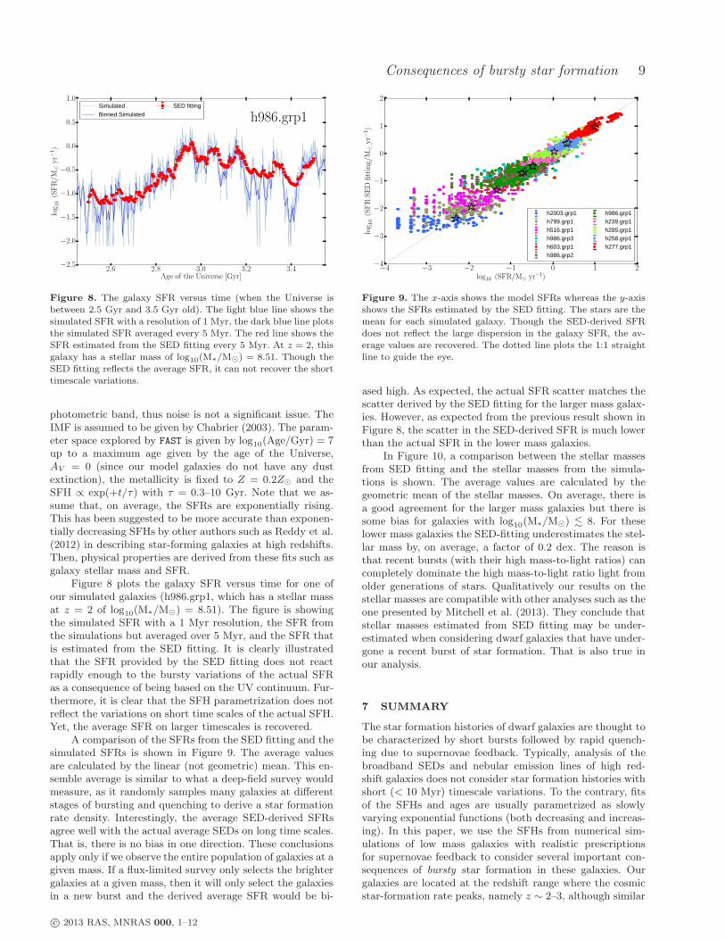
photometric band, thus noise is not a significant issue. TheIMF is assumed to be given by Chabrier (2003). The param-eter space explored by FAST is given by log10(Age/Gyr) = 7up to a maximum age given by the age of the Universe,AV = 0 (since our model galaxies do not have any dustextinction), the metallicity is fixed to Z = 0.2Z⊙ and theSFH ∝ exp(+t/τ ) with τ = 0.3–10 Gyr. Note that we as-sume that, on average, the SFRs are exponentially rising.This has been suggested to be more accurate than exponen-tially decreasing SFHs by other authors such as Reddy et al.(2012) in describing star-forming galaxies at high redshifts.Then, physical properties are derived from these fits such asgalaxy stellar mass and SFR.

Figure 8 plots the galaxy SFR versus time for one ofour simulated galaxies (h986.grp1, which has a stellar massat z = 2 of log10(M∗/M⊙) = 8.51). The figure is showingthe simulated SFR with a 1 Myr resolution, the SFR fromthe simulations but averaged over 5 Myr, and the SFR thatis estimated from the SED fitting. It is clearly illustratedthat the SFR provided by the SED fitting does not reactrapidly enough to the bursty variations of the actual SFRas a consequence of being based on the UV continuum. Fur-thermore, it is clear that the SFH parametrization does notreflect the variations on short time scales of the actual SFH.Yet, the average SFR on larger timescales is recovered.

A comparison of the SFRs from the SED fitting and thesimulated SFRs is shown in Figure 9. The average valuesare calculated by the linear (not geometric) mean. This en-semble average is similar to what a deep-field survey wouldmeasure, as it randomly samples many galaxies at differentstages of bursting and quenching to derive a star formationrate density. Interestingly, the average SED-derived SFRsagree well with the actual average SEDs on long time scales.That is, there is no bias in one direction. These conclusionsapply only if we observe the entire population of galaxies at agiven mass. If a flux-limited survey only selects the brightergalaxies at a given mass, then it will only select the galaxiesin a new burst and the derived average SFR would be bi-

−4 −3 −2 −1 0 1 2log10 (SFR/M⊙ yr−1)

−4

−3

−2

−1

0

1

2

log 1

0(SFRSEDfitting/M

⊙yr

−1)



Figure 9. The x-axis shows the model SFRs whereas the y-axisshows the SFRs estimated by the SED fitting. The stars are themean for each simulated galaxy. Though the SED-derived SFRdoes not reflect the large dispersion in the galaxy SFR, the av-erage values are recovered. The dotted line plots the 1:1 straightline to guide the eye.

ased high. As expected, the actual SFR scatter matches thescatter derived by the SED fitting for the larger mass galax-ies. However, as expected from the previous result shown inFigure 8, the scatter in the SED-derived SFR is much lowerthan the actual SFR in the lower mass galaxies.

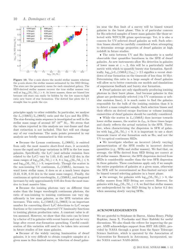
In Figure 10, a comparison between the stellar massesfrom SED fitting and the stellar masses from the simula-tions is shown. The average values are calculated by thegeometric mean of the stellar masses. On average, there isa good agreement for the larger mass galaxies but there issome bias for galaxies with log10(M∗/M⊙) . 8. For theselower mass galaxies the SED-fitting underestimates the stel-lar mass by, on average, a factor of 0.2 dex. The reason isthat recent bursts (with their high mass-to-light ratios) cancompletely dominate the high mass-to-light ratio light fromolder generations of stars. Qualitatively our results on thestellar masses are compatible with other analyses such as theone presented by Mitchell et al. (2013). They conclude thatstellar masses estimated from SED fitting may be under-estimated when considering dwarf galaxies that have under-gone a recent burst of star formation. That is also true inour analysis.

7 SUMMARY

The star formation histories of dwarf galaxies are thought tobe characterized by short bursts followed by rapid quench-ing due to supernovae feedback. Typically, analysis of thebroadband SEDs and nebular emission lines of high red-shift galaxies does not consider star formation histories withshort (< 10 Myr) timescale variations. To the contrary, fitsof the SFHs and ages are usually parametrized as slowlyvarying exponential functions (both decreasing and increas-ing). In this paper, we use the SFHs from numerical sim-ulations of low mass galaxies with realistic prescriptionsfor supernovae feedback to consider several important con-sequences of bursty star formation in these galaxies. Ourgalaxies are located at the redshift range where the cosmicstar-formation rate peaks, namely z ∼ 2–3, although similar

c© 2013 RAS, MNRAS 000, 1–12


6.5 7.0 7.5 8.0 8.5 9.0 9.5 10.0log10 (M∗/M⊙)

6.5

7.0

7.5

8.0

8.5

9.0

9.5

10.0

log 1

0(M

∗SEDfitting/M

⊙)



Figure 10. The x-axis shows the model stellar masses whereasthe y-axis shows the stellar masses estimated by the SED fitting.The stars are the geometric mean for each simulated galaxy. TheSED-derived stellar masses recover the true stellar masses verywell at log10(M∗/M⊙) > 8. At lower masses, these are biased lowbecause old stars can easily be hidden by the low mass-to-lightratio new burst of star formation. The dotted line plots the 1:1straight line to guide the eye.

principles apply to other redshifts. In particular, we analysethe Lν(1500A)/Lν(900A) ratio and the Lyα and Hα EWs.The star-forming main sequence is investigated as well in thestellar mass range of around 107–1010 M⊙. We stress thatthe values reported in this analysis are rest-frame and thatdust extinction is not included. This fact will not changeany of our conclusions. The main points presented in ouranalysis are briefly summarized in this section.

• Because the Lyman continuum, Lν(900A), is emittedfrom only the most massive short-lived stars, it accuratelytraces the rapid and large variations in SFR in the low massgalaxies. Specifically, the LyC (and nebular emission linesrelated to the LyC) vary by 1.03, 0.45, and 0.22 dex in themass ranges of log10(M∗/M⊙) < 8, 8 6 log10(M∗/M⊙) 6 9,and log10(M∗/M⊙) > 9, respectively. Though the scatter inthe non-ionizing UV continuum, Lν(1500A), increases to-ward lower stellar mass, it does so at a much lower degree(0.43, 0.28, 0.16 dex in the same mass ranges). Finally, thecontinuum at optical wavelengths, Lν(5500A), and longwardincreases by only approximately 0.05 dex from the most mas-sive to least massive bins.

• Because the ionizing photons vary on different timescales than the longer wavelength continuum photons, theratio of non-ionizing to ionizing continuum can vary sig-nificantly in low mass galaxies, as the SFR variation alsoincreases. This ratio, Lν(1500A)/Lν(900A) is an importantnumber for converting direct LyC detections to LyC escapefractions or for converting observed UV luminosity functionsto ionizing photon production rates. A constant value is of-ten assumed. However, we show that this ratio can be lowerby a factor of 2 in galaxies with recent bursts and can be verylarge after recent star-formation quenching. Careful consid-eration of this variation will need to be taken into accountin future studies of low mass galaxies.

• Because of the widely varying luminosities of dwarfgalaxies, it is very difficult to obtain complete samples at agiven mass in flux-limited surveys. Selection of dwarf galax-

ies near the flux limit of a survey will be biased towardgalaxies in the burst phase. This is of particular concernfor Hα-selected samples of lower mass galaxies like those se-lected with WFC3/IR grism spectroscopy. Yet, it is also aconcern for UV-selected dwarf galaxies as well. Such selec-tion biases should be carefully considered when attemptingto determine average properties of dwarf galaxies at highredshift in future studies.

• The ratio between UV and Hα luminosity is a usefulobservable that quantifies burstiness in the SFH of dwarfgalaxies. As new instruments allow Hα detection in galaxiesof lower mass at z ∼ 2, this will be a particularly usefulmetric with which to quantify bursty star formation. Specif-ically, log10[νLν(1500A)/LHα] > 2.5 signifies a recent shut-down of star formation on the timescale of less than 10 Myr.Determining this ratio in a large sample of dwarf galaxieswill allow us to better constrain our models and simulationsof supernovae feedback and bursty star formation.

• Dwarf galaxies are only significantly producing ionizingphotons in their burst phase. And because galaxies in thisphase are preferentially selected (via UV continuum or neb-ular emission lines), it is much easier to find the galaxiesresponsible for the bulk of the ionizing emission than it isto detect a mass complete sample. Such selection biases andtheir effects on derived escape fractions or volume ionizingemissivities of dwarf galaxies should be carefully considered.

• While the scatter in Lν(1500A) does increase towardslower stellar masses, the scatter in LHα is three times largerand closely reflects the actual variation in the SFR. There-fore, when characterizing the dispersion in SFR of galax-ies with log10(M∗/M⊙) < 9, it is important to use a shorttimescale tracer of star formation such as Hα, and not theUV-to-optical continuum SEDs.

• We investigate whether an incorrect (slowly varying)parametrization of the SFH results in incorrect derivedquantities (e.g., SFRs and stellar masses). We find that, onaverage, the SFRs derived from SED fitting are correct atall stellar masses. However, the SFR dispersion derived fromSEDs is considerably smaller than the true SFR dispersionin these galaxies. These conclusions apply only if we samplethe entire population of galaxies at a given mass, otherwisethe SFR will be overestimated as flux-limited surveys willbe biased toward selecting galaxies in a burst phase.

• On average, for galaxies with log10(M∗/M⊙) > 8, thestellar masses from SED fitting are correct. However, forgalaxies with log10(M∗/M⊙) < 8, we find that stellar massesare underpredicted by the SED fitting by a factor 0.2 dexwhen assuming slowly varying SFHs.

ACKNOWLEDGEMENTS

We are grateful to Stephane de Barros, Alaina Henry, PhilipHopkins, Jason X. Prochaska and Marc Rafelski for usefuldiscussions. We also thank the referee for improving the pa-per. AMB acknowledges support from HST AR-12631, pro-vided by NASA through a grant from the Space TelescopeScience Institute, which is operated by the Association ofUniversities for Research in Astronomy, Incorporated, un-der NASA contract NAS5-26555.

c© 2013 RAS, MNRAS 000, 1–12


REFERENCES

Alavi A. et al., 2014, ApJ, 780, 143Atek H., et al., 2010, ApJ, 723, 104Atek H. et al., 2011, ApJ, 743, 121Atek H., et al., 2014, ApJ, 789, 96Becker G. D., Bolton J. S., 2013, MNRAS, 436, 1023Beckwith S. V. W., et al., 2006, AJ, 132, 1729Behroozi P. S., Wechsler R. H., Conroy C., 2013, ApJ, 770,57

Belli S., Jones T., Ellis R. S., Richard J., 2013, ApJ, 772,141

Bigiel F., Leroy A., Walter F., Blitz L., Brinks E., de BlokW. J. G., Madore B., 2010, AJ, 140, 1194

Bigiel F., Leroy A., Walter F., Brinks E., de Blok W. J. G.,Madore B., Thornley M. D., 2008, AJ, 136, 2846

Blanc G. A., Heiderman A., Gebhardt K., Evans II N. J.,Adams J., 2009, ApJ, 704, 842

Boquien M., Buat V., Perret V., 2014, A&A, 571, A72Boselli A., Boissier S., Cortese L., Buat V., Hughes T. M.,Gavazzi G., 2009, ApJ, 706, 1527

Brammer G. B., et al., 2012, ApJS, 200, 13Brinchmann J., Charlot S., White S. D. M., Tremonti C.,Kauffmann G., Heckman T., Brinkmann J., 2004, MN-RAS, 351, 1151

Brooks A. M., Governato F., Booth C. M., Willman B.,Gardner J. P., Wadsley J., Stinson G., Quinn T., 2007,ApJ, 655, L17

Brooks A. M., et al., 2011, ApJ, 728, 51Brooks A. M., Zolotov A., 2014, ApJ, 786, 87Bruzual G., Charlot S., 2003, MNRAS, 344, 1000 (BC03)Ceverino D., Klypin A., Klimek E. S., Trujillo-Gomez S.,Churchill C. W., Primack J., Dekel A., 2014, MNRAS,442, 1545

Chabrier G., 2003, ApJL, 586, L133Christensen C., Quinn T., Governato F., Stilp A., Shen S.,Wadsley J., 2012, MNRAS, 425, 3058

Christensen C., Governato F., Quinn T., Brooks A. M.,Fisher D. B., Shen S., McCleary J., Wadsley J., 2014,MNRAS, 440, 2843

da Silva R. L., Fumagalli M., Krumholz M., 2012, ApJ,745, 145

da Silva R. L., Fumagalli M., Krumholz M. R., 2014, MN-RAS, 444, 3275

Domınguez A., et al., 2013, ApJ, 763, 145Forero-Romero J. E., Dijkstra M., 2013, MNRAS, 428, 2163Fumagalli M., da Silva R. L., Krumholz M. R., 2011, ApJL,741, L26

Giavalisco M., et al., 2004, ApJ, 600, L93Gill S. P. D., Knebe A., Gibson B. K., 2004, MNRAS, 351,399

Glazebrook K., Blake C., Economou F., Lilly S., CollessM., 1999, MNRAS, 306, 843

Governato F. et al., 2012, MNRAS, 422, 1231Gronwall C. et al., 2007, ApJ, 667, 79Haardt F., Madau P., 2001, in Neumann D. M., TranJ. T. V., eds, Clusters of Galaxies and the High RedshiftUniverse Observed in X-rays. , arXiv:astro-ph/0106018

Haardt F., Madau P., 2012, ApJ, 746, 125Henry A., et al., 2013, ApJ, 776, L27Hopkins P. F., Keres D., Onorbe J., Faucher-Giguere C.-A., Quataert E., Murray N., Bullock J. S., 2014, MNRAS,

445, 581Iglesias-Paramo J., Boselli A., Gavazzi G., Zaccardo A.,2004, A&A, 421, 887

Knollmann S. R., Knebe A., 2009, ApJS, 182, 608Kriek M., van Dokkum P. G., Labbe I., Franx M., Illing-worth G. D., Marchesini D., Quadri R. F., 2009, ApJ, 700,221

Krueger H., Fritze-v. Alvensleben U., Loose H.-H., 1995,A&A, 303, 41

Leroy A. K., Walter F., Brinks E., Bigiel F., de BlokW. J. G., Madore B., Thornley M. D., 2008, AJ, 136,2782

Meurer G. R. et al., 2009, ApJ, 695, 765Mitchell P. D., Lacey C. G., Baugh C. M., Cole S., 2013,MNRAS, 435, 87

Mostardi R. E., Shapley A. E., Nestor D. B., Steidel C. C.,Reddy N. A., Trainor R. F., 2013, ApJ, 779, 65

Munshi F. et al., 2013, ApJ, 766, 56Nestor D. B., Shapley A. E., Kornei K. A., Steidel C. C.,Siana B., 2013, ApJ, 765, 47

Nestor D. B., Shapley A. E., Steidel C. C., Siana B., 2011,ApJ, 736, 18

Nilsson K. K., Tapken C., Møller P., Freudling W., FynboJ. P. U., Meisenheimer K., Laursen P., Ostlin G., 2009,A&A, 498, 13

Noeske K. G. et al., 2007a, ApJL, 660, L47Noeske K. G. et al., 2007b, ApJL, 660, L43Osterbrock D. E., Ferland G. J., 2006, Astrophysics ofgaseous nebulae and active galactic nuclei

Ouchi M. et al., 2008, ApJS, 176, 301Pacifici C., Charlot S., Blaizot J., Brinchmann J., 2012,MNRAS, 421, 2002

Pannella M. et al., 2009, ApJL, 698, L116Prochaska J. X., Worseck G., O’Meara J. M., 2009, ApJ,705, L113

Reddy N. A., Steidel C. C., 2009, ApJ, 692, 778Reddy N. A., Pettini M., Steidel C. C., Shapley A. E., ErbD. K., Law D. R., 2012, ApJ, 754, 25

Sanders R. L., et al., 2015, ApJ, 799, 138Schruba A. et al., 2011, AJ, 142, 37Shen S., Wadsley J., Stinson G., 2010, MNRAS, 407, 1581Shen S., Madau P., Conroy C., Governato F., Mayer L.,2014, ApJ, 792, 99

Siana B. et al., 2007, ApJ, 668, 62Siana B. et al., 2010, ApJ, 723, 241Speagle J. S., Steinhardt C. L., Capak P. L., SilvermanJ. D., 2014, ApJS, 214, 15

Spergel D. N. et al., 2007, ApJS, 170, 377Stark D. et al., 2014, MNRAS, 445, 3200Steidel C. C., Pettini M., Adelberger K. L., 2001, ApJ, 546,665

Stinson G., Seth A., Katz N., Wadsley J., Governato F.,Quinn T., 2006, MNRAS, 373, 1074

Stinson G. S., Dalcanton J. J., Quinn T., Kaufmann T.,Wadsley J., 2007, ApJ, 667, 170

Teyssier R., Pontzen A., Dubois Y., Read J. I., 2013, MN-RAS, 429, 3068

Trujillo-Gomez S., et al., MNRAS, 446, 1140van der Wel A. et al., 2011, ApJ, 742, 111Vanzella E., et al., 2010, ApJ, 725, 1011Wadsley J. W., Stadel J., Quinn T., 2004, New Astronomy,9, 137

c© 2013 RAS, MNRAS 000, 1–12

http://arxiv.org/abs/astro-ph/0106018


Weisz D. R. et al., 2012, ApJ, 744, 44Whitaker K. E., van Dokkum P. G., Brammer G., FranxM., 2012, ApJL, 754, L29

Whitaker K. E., et al., 2014, ApJ, 795, 104Zolotov A. et al., 2012, ApJ, 761, 71

c© 2013 RAS, MNRAS 000, 1–12

consequencesofburstystar formationon galaxy observablesat ... · consequencesofburstystar...

Documents