consistent specification tests for ordered discrete …

1

CONSISTENT SPECIFICATION TESTS FOR ORDERED DISCRETE CHOICE MODELS*

Juan Mora and Ana I. Moro-Egido**

WP-AD 2006-17

Correspondence to: Juan Mora. Departamento de Fundamentos del Análisis Económico, Universidad de Alicante, Apartado de Correos 99, 03080 Alicante, Spain. E-mail address: [email protected]. Editor: Instituto Valenciano de Investigaciones Económicas, S.A. Primera Edición Julio 2006 Depósito Legal: V-3367-2006 IVIE working papers offer in advance the results of economic research under way in order to encourage a discussion process before sending them to scientific journals for their final publication.

* We are grateful to M.D. Collado, C. Muller and F. Peñaranda for helpful comments. Financial support from Spanish MEC (SEJ2005-02829/ECON) and Ivie is gratefully acknowledged. **J. Mora: Universidad de Alicante. A.I. Moro-Egido: Universidad de Granada.

CONSISTENT SPECIFICATION TESTS FOR ORDERED DISCRETE CHOICE MODELS

Juan Mora and Ana I. Moro-Egido

ABSTRACT

We discuss how to test consistently the specification of an ordered discrete

choice model. Two approaches are considered: tests based on conditional moment

restrictions and tests based on comparisons between parametric and

nonparametric estimations. Following these approaches, various statistics are

proposed and their asymptotic properties are discussed. The performance of the

statistics is compared by means of simulations. A variant of the standard

conditional moment statistic and a generalization of Horowitz-Spokoiny’s statistic

perform best.

Codes JEL: C25, C52, C15.

Keywords: Specification Tests, Ordered Discrete Choice Models; Statistical Simulation.

1. INTRODUCTION

Ordered discrete choice variables often appear in Statistics and Econometrics

as a dependent variable. The outcomes of an ordered discrete choice variable

Y are usually labelled as 0, 1, ..., J . Given certain explanatory variables X =

(X1, ...,Xk)0, the researcher is usually interested in analysing whether one (or

some) of the proposed explanatory variables is significant or not, and/or providing

accurate estimates of the conditional probabilities Pr(Y = j | X = x), which

may be interesting by themselves or required in a first stage to derive a two-stage

estimator. Examples of ordered discrete choice dependent variables that have been

used in applied work include: education level attained by individuals (Jiménez and

Kugler 1987); female labour participation: work full-time, work part-time, not to

work (Gustaffson and Stafford 1992); level of demand for a new product or service

(Klein and Sherman 1997); and number of children in a family (Calhoun 1989).

The parametric model that is most frequently used for an ordered discrete choice

variable arises when one assumes the existence of a latent continuous dependent

variable Y ∗ for which a linear regression model Y ∗ = X 0β0 + u holds; the non-

observed variable Y ∗ and the observed variable Y are assumed to be related as

follows:

Y = j if µ0,j−1 ≤ Y ∗ < µ0j, for j = 0, 1, ..., J, (1)

where µ0,−1 ≡ −∞, µ0,J ≡ +∞ and µ00, µ01, ..., µ0,J−1 are threshold parameters

such that µ00 ≤ µ01 ≤ ... ≤ µ0,J−1. Assuming independence between u and X, the

relationship (1) induces the following specification for Y :

Pr(Y = j | X) = F (µ0j −X 0β0)− F (µ0,j−1 −X 0β0), for j = 0, 1, ..., J, (2)

where F (·) is the distribution function of u, usually referred to as the “link func-

1

tion”. In a parametric framework, for the sake of identification of the model it

is usually assumed that the first threshold parameter µ00 is zero; additionally

it is assumed that F (·) is entirely known, the most typical choices being the

standard normal distribution (“ordered probit model”) and the logistic distrib-

ution (“ordered logit model”). With these assumptions we obtain a full para-

meterization of the conditional distribution Y | X = x, with parameter vector

θ0 = (β00, µ

00)0 ∈ Θ ⊂ Rk+J−1.

The key assumptions in a parametric ordered discrete choice model are the

linearity in the latent regression model, the form of the link function F (·) (specif-

ically, its symmetry and its behaviour at the tails) and the independence between

u and X in the latent regression model (which, in turn, implies that it is ho-

moskedastic). Parameter estimates and predicted probabilities based on ordered

discrete choice models are inconsistent if any of these key assumptions is not met

(note that in contrast to standard regression models, heteroskedasticity or mis-

specification of the distribution function of u provoke inconsistencies). On the

other hand, there exist semiparametric methods (Klein and Sherman 2002) and

even nonparametric methods (Matzkin 1992) that allow for consistent estimation

of the conditional probabilities Pr(Y = j | X = x) under much weaker assump-

tions; these methods have not been much used in empirical applications due their

technical complexity, but they provide a reasonable alternative to purely para-

metric methods. Therefore, it is especially important to test the specification of

a parametric ordered discrete choice model, since misspecification errors lead to

inconsistent estimation, and it is possible to use alternative consistent techniques.

In recent years, various statistics have been proposed to test one (or some) of

the assumptions of a parametric ordered discrete choice model. However, most

2

of these statistics are constructed to detect only specific departures from the null

hypothesis; for example, Weiss (1997) proposes to test the null of a homoskedastic

u versus some parametric heteroskedastic alternatives; Glewwe (1997) proposes

to test the null that u is normal versus the alternative that it is a member of

the Pearson family; Murphy (1996) proposes to test the null that F (·) is logistic

versus various alternatives; and Santos Silva (2001) proposes a test statistic to face

two non-nested parametric specifications. By contrast, we focus here on consistent

specification test statistics, i.e. test statistics that allow us to detect any deviation

from the null hypothesis “the proposed parametric specification is correct”.

Roughly speaking, two main approaches may be followed in our context to de-

rive consistent specification statistics: tests based on conditional moment (CM)

restrictions, which can be constructed following the general methodology described

in Newey (1985), Tauchen (1985) and Andrews (1988); and tests based on compar-

isons between parametric and nonparametric estimations, such as those proposed

by Andrews (1997), Stute (1997) and Horowitz and Spokoiny (2001), among oth-

ers. The objective of this article is to examine how these two approaches can

be applied to test the specification of an ordered discrete choice model, and to

compare the performance of the resulting statistics by means of simulations.

Our results highlight the importance of covariance matrix estimation in CM

tests. Specifically, standard CM statistics, computed with covariance matrix es-

timators based on actual derivatives, usually perform worse than statistics based

on comparisons between parametric and nonparametric estimations. However, ex-

ploiting the information about conditional expectations contained in the model,

here we derive variants of standard CM statistics that perform much better than

standard CM statistics; additionally, these variants are easy to compute, since

3

they can be obtained using artificial regressions. On the other hand, our results

suggest that the methodology proposed in Horowitz and Spokoiny (2001) can be

extended successfully to the context of ordered discrete choice models, and the

resulting statistic outperforms other statistics that are based on comparisons be-

tween parametric and nonparametric methods. However, when we compare the

performace of the generalization of Horowitz-Spokoiny’s statistic with the variant

of the standard CM statistic that we propose to use, there is no clear-cut answer

to the question of which one performs better: the latter outperforms the former in

some cases (e.g. with heteroskedastic alternatives) and is computationally much

less demanding, but the additional power that is obtained when using the former

in some other cases (e.g. with non-normal alternatives) may well justify the extra

computing effort.

The rest of the paper is organized as follows. In Sections 2 and 3 we describe

the test statistics considered here. In Section 4 we report the results of various

Monte Carlo experiments. In Section 5 we present two empirical applications. In

Section 6 we conclude. Some technical details are relegated to an Appendix.

2. STATISTICS BASED ON CONDITIONAL MOMENT

RESTRICTIONS

We assume that independent and identically distributed (i.i.d.) observations

(Yi, X0i)0 are available, where, hereafter, i = 1, ..., n. Additionally, the following

notation will be used: Dji ≡ I(Yi = j), for j = 0, 1, ..., J , where I(·) is the

indicator function; and, given θ ≡ (β0, µ0)0 ∈ Θ ⊂ Rk+J−1, p0i(θ) ≡ F (−X 0iβ);

pJi(θ) ≡ 1− F (µJ−1 −X 0iβ); if J ≥ 2, p1i(θ) ≡ F (µ1 −X 0

iβ)− F (−X 0iβ); and if

J ≥ 3, pji(θ) ≡ F (µj −X 0iβ)− F (µj−1 −X 0

iβ), for j = 2, ..., J − 1.

4

Let us consider mji(θ) ≡ Dji − pji(θ). Then, it follows from (2) that

E{mji(θ0) | Xi} = 0, for j = 0, 1, ..., J. (3)

This yields J + 1 conditional moment restrictions that must be satisfied. In

fact, since the sum of all probabilities adds to one, only J moment conditions

are relevant to construct a test statistic. Specifically, we disregard the moment

condition for j = 0 and consider the random vectorPn

i=1mi(bθ), where mi(θ) is

the J × 1 column vector whose j-th component is mji(θ) and bθ is a well-behavedestimator of θ0. To derive an asymptotically valid test statistic, we must analyze

the asymptotic behaviour ofPn

i=1mi(bθ). First of all note that using a first-orderTaylor expansion of mji(bθ)−mji(θ0), it follows that

n−1/2nXi=1

mi(bθ) = n−1/2nXi=1

mi(θ0) +B0 × n1/2(bθ − θ0) + op(1), (4)

whereB0 ≡ E{Bi(θ0)} andBi(θ) denotes the J×(k+J−1)matrix whose j-th row

is ∂mji(θ)/∂θ0. Thus, the asymptotic behaviour of n−1/2

Pni=1mi(bθ) depends on

the asymptotic behaviour of n1/2(bθ−θ0). In our context, since our null hypothesisspecifies the conditional distribution Yi | Xi = x, the natural way to estimate θ0

is maximum likelihood (ML). The log-likelihood of the model can be written as

lnL(θ) =nXi=1

JXj=0

Dji ln pji(θ).

We assume that the regularity conditions that ensure that the ML estimator is

asymptotically normal are met (see e.g. Amemiya 1985, Chapter 9). In this case,

this amounts to saying that the ML estimator bθ satisfiesn1/2(bθ − θ0) = A

−10 × n−1/2

nXi=1

gi (θ0) + op(1), (5)

5

where gi(θ) ≡PJ

j=1Dji∂ ln pji(θ)/∂θ is the derivative with respect to θ of the i-th

term in lnL(θ), and A0 is the limiting information matrix, i.e. A0 = E{Ai(θ0)},

for Ai(θ) ≡ −∂gi(θ)/∂θ0. From (4) and (5) it follows that:

n−1/2nXi=1

mi(bθ) = [IJ : B0A−10 ]⎡⎢⎣ n−1/2

Pni=1mi(θ0)

n−1/2Pn

i=1 gi (θ0)

⎤⎥⎦+ op(1),

where IJ is the J × J identity matrix. Hence,

n−1/2nXi=1

mi(bθ) d−→ N (0,V0) , (6)

where

V0 ≡ [IJ : B0A−10 ]Q0[IJ : B0A−10 ]

0, (7)

Q0 ≡ E{Qi(θ0)} and Qi(θ) ≡ (mi(θ)0,gi(θ)

0)0(mi(θ)0,gi(θ)

0). Finally, to derive

a test statistic, a consistent estimator of V0 must be proposed. It is worthwhile

discussing in detail how V0 can be estimated, since it is well-known that the

finite-sample performance of statistics based on conditional moment restrictions

crucially depends on this.

According to (7), the natural candidate for estimating V0 is Vn,1 ≡ [IJ :

BnA−1n ]Qn [IJ : BnA

−1n ]

0, where Qn ≡ n−1Pn

i=1Qi(bθ), Bn ≡ n−1Pn

i=1Bi(bθ)and An ≡ n−1

Pni=1Ai(bθ). However, following the literature on artificial re-

gressions (see e.g. MacKinnon 1992), it is possible to propose an alternative

estimator of V0 that leads to a computationally simpler statistic. To derive

it, note that E{mli(θ)gi(θ)0} = E{pli∂ ln pli(θ)/∂θ0} = E{−∂mli(θ)/∂θ

0}; hence

E{mi(θ0)gi(θ0)0} = −B0. Moreover, the information matrix equality ensures that

E{gi(θ0)gi(θ0)0} = A0. Using these equalities, it follows that V0 equals

E{mi(θ0)mi(θ0)0}−E{mi(θ0)gi(θ0)

0}E{gi(θ0)gi(θ0)0}−1E{gi(θ0)mi(θ0)0}. (8)

6

This leads us to consider

Vn,2 ≡ n−1[nXi=1

mi(bθ)mi(bθ)0 − nXi=1

mi(bθ)gi(bθ)0{ nXi=1

gi(bθ)gi(bθ)0}−1 nXi=1

gi(bθ)mi(bθ)0].Vn,1 and Vn,2 are the standard choices for estimating V0. Both are obtained

by simply replacing population moments by sample moments. However, in our

context we can do better than that. Observe that our null hypothesis yields the

specification of the conditional distribution Y | X = x. This means that we can

compute the conditional expectation with respect to the independent variables

and then, by the law of iterated expectations, the sample analog of this condi-

tional expectation is a consistent estimator of the the population moment; e.g.

E{mi(θ0)mi(θ0)0} can be consistently estimated with n−1

Pni=1EX{mi(bθ)mi(bθ)0}.

Following this approach, expression (8) for V0 suggests that we can estimate this

matrix with Vn,3 ≡ n−1Pn

i=1Vi,3(bθ), whereVi,3(θ) ≡ EX{mi(θ)mi(θ)

0}−EX{mi(θ)gi(θ)0}EX{gi(θ)gi(θ)0}−1EX{gi(θ)mi(θ)

0}.

Observe that the analytical expressions of these conditional expectations are easy

to derive. On the other hand, this approach could also be followed using expression

(7) rather than (8) as a starting point; but the estimator that is obtained in this

way proves to be again Vn,3.

To sum up, we can consider three possible consistent estimates for V0 and,

thus, we can derive three possible test statistics

C(M)n,l ≡ n−1{

nXi=1

mi(bθ)0}{Vn,l}−1{nXi=1

mi(bθ)},for l = 1, 2, 3. From (6), it follows that if specification (2) is correct then C(M)

n,l

d−→

χ2J ; hence, given a significance level α, an asymptotically valid critical region is

7

{C(M)n,l > χ21−α;J}, where χ21−α;J is the 1 − α quantile of a χ2J distribution. To

facilitate the computation of these three statistics, in Appendix A1 we derive the

specific analytical expressions forVn,1,Vn,2 andVn,3 that are obtained here. As is

well-known in the relevant literature, note that C(M)n,2 can also be computed using

an artificial regression because, sincePn

i=1 gi(bθ) = (∂ lnL/∂θ)|θ=bθ = 0, the statis-

tic C(M)n,2 proves to be the explained sum of squares in the artificial regression of a

vector of ones on mi(bθ)0 and gi(bθ). On the other hand, using a Cholesky decom-position of EX{mi(θ)mi(θ)

0}, it is also possible to derive an artificial regression

whose explained sum of squares coincides with C(M)n,3 (see Appendix A2).

Still within the framework of tests based on conditional moment restrictions,

more statistics can be derived following the methodology described in Andrews

(1988), who proposes increasing the degrees of freedom of the statistic by parti-

tioning the support of the regressors. Specifically, let us assume that the support

of Xi is partitioned into G subsets A1, ..., AG. Then we can define mjgi(θ) ≡

mji(θ)I(Xi ∈ Ag) for j = 1, ..., J and g = 1, ..., G, and thus consider the JG

conditional moment restrictions

E{mji(θ0) | Xi} = 0, for j = 1, ..., J, and g = 1, ..., G.

To derive a test statistic, we consider now the random vectorPn

i=1m(P )i (bθ), where

m(P )i (θ) ≡mi(θ)⊗Pi, and Pi is the G× 1 matrix whose g-th row is I(Xi ∈ Ag).

As before, it follows that

n−1/2nXi=1

m(P )i (bθ) d−→ N(0,V

(P )0 ), (9)

where V(P )0 ≡ [IJG : B(P )0 A−10 ]Q

(P )0 [IJG : B

(P )0 A−10 ]

0, B(P )0 ≡ E{B(P )i (θ0)}, Q(P )

0 ≡

E{Q(P )i (θ0)}, B(P )i (θ) ≡ Bi(θ) ⊗ Pi and Q

(P )i (θ) ≡ (m

(P )i (θ)0,gi(θ)

0)0(m(P )i (θ)0,

8

gi(θ)0). Now, the natural candidate for estimatingV(P )

0 isV(P )n,1 ≡ [IJG : B

(P )n A−1n ]Q

(P )n

[IJG : B(P )n A−1n ]

0, where B(P )n ≡ n−1Pn

i=1B(P )i (bθ) and Q(P )

n ≡ n−1Pn

i=1Q(P )i (bθ).

With the same reasoning as before, two other consistent estimators of V(P )0 can be

proposed: V(P )n,2 and V

(P )n,3 , defined in the same way as Vn,2 and Vn,3, respectively,

but replacingmi(bθ) bym(P )i (bθ) (see Appendix A1). In this fashion we again obtain

three different test statistics

C(MP )n,l ≡ n−1{

nXi=1

m(P )i (bθ)0}{V(P )

n,l }−1{nXi=1

m(P )i (bθ)},

for l = 1, 2, 3. From (9), it follows that if specification (2) is correct thenC(MP )n,l

d−→

χ2JG; hence, C(MP )n,l can also be used as a test statistic. Additionally, both C

(MP )n,2

and C(MP )n,3 can be computed using an artificial regression. Specifically, C(MP )

n,2

coincides with the explained sum of squares in the artificial regression of a vector

of ones on m(P )i (bθ) and gi(bθ), whereas the artificial regression which allows us to

compute C(MP )n,3 is described in Appendix A2.

Finally, when J ≥ 2 and k ≥ 2, Butler and Chatterjee (1997) propose using a

test of overidentifying restrictions. Observe that (3) implies that the following Jk

moment conditions hold:

E{Xlimji(θ0)} = 0, for l = 1, ..., k, j = 1, ..., J,

where Xli denotes the l-th component of Xi. Since the number of parameters is

k + J − 1, a test of overidentifying restrictions is possible if Jk > k + J − 1, and

this condition holds if and only if J ≥ 2 and k ≥ 2. Adapting the general results

of the generalized method of moments tests to our framework (see e.g. Hamilton

1994, Chapter 14), it follows that now the test of overidentifying restrictions can

be computed as follows: i) obtain an initial estimate of θ0, say θ, by minimizing

9

sn(θ)0sn(θ), where sn(θ) ≡ n−1

Pni=1mi(θ)⊗Xi; ii) compute Sn(θ), where

Sn(θ) ≡

⎡⎢⎢⎢⎢⎢⎣S11,n(θ) ... S1J,n(θ)

... ... ...

SJ1,n(θ) ... SJJ,n(θ)

⎤⎥⎥⎥⎥⎥⎦ ,Sjj,n(θ) = n−1

Pni=1XiX

0ipji(1− pji) and Sjl,n(θ) = −n−1

Pni=1XiX

0ipjipli for j 6=

l; iii) obtain a final estimate of θ0, say eθ, by minimizing sn(θ)0Sn(θ)−1sn(θ); andiv) compute the test statistic

C(BC)n = nsn(eθ)0Sn(θ)−1sn(eθ).

If specification (2) is correct then C(BC)n

d−→ χ2Jk−(k+J−1); thus, C(BC)n can also be

used as a statistic to perform an asymptotically valid specification test.

3. STATISTICS BASED ON COMPARISONS BETWEEN

PARAMETRIC AND NONPARAMETRIC ESTIMATIONS

Many specification tests have recently been developed using comparisons be-

tween parametric and nonparametric estimations. In this paper we consider three

of them: one based on the comparison of joint empirical distribution functions

(Andrews 1997), and two others based on comparisons between regression esti-

mations, either non-smoothed (Stute 1997) or smoothed (Horowitz and Spokoiny

2001). In fact, as we discuss below, only the first of these statistics applies directly

to our framework, but the other two can be conveniently modified to cover our

problem. We focus on these three statistics because they have the advantage that

their performance does not depend on the choice of a bandwidth value1. Note as1The test statistics proposed by Andrews (1997) and Stute (1997) do not use any bandwidth.

Horowitz and Spokoiny (2001) propose using as a test statistic a maximum from among statistics

computed with different bandwidths; hence the influence of bandwidth selection is ruled out.

10

well that these three statistics require the use of a root-n-consistent estimator of

θ0; as in the previous section, the ML estimator is the natural choice.

Andrews (1997) suggests testing a parametric specification of the conditional

distribution Y | X = x by comparing the joint empirical distribution function of

(Y,X 0)0 and an estimate of the joint distribution function based on the parametric

specification. Specifically, if F (· | x, θ0) is the assumed parametric conditional

distribution function of Y | X = x and we denote

Hn(x, y) ≡ n−1{nXi=1

I(Yi ≤ y,Xi ≤ x)−nXi=1

F (y | Xi,bθ)I (Xi ≤ x)},

where bθ is a root-n-consistent estimator of θ0, Andrews (1997) proposes using theKolmogorov-Smirnov-type test statistic:

C(AN)n ≡ max

1≤j≤n

¯n1/2Hn(Xj, Yj)

¯.

The asymptotic null distribution of C(AN)n cannot be tabulated but, given a sig-

nificance level α, an asymptotically valid critical region is {C(AN)n > c

(AN)α,n }, where

c(AN)α,n is a bootstrap critical value. This bootstrap critical value can be obtained

as the 1 − α quantile of {C(AN)∗n,b , b = 1, ..., B}, where C(AN)∗

n,b is a bootstrap sta-

tistic constructed in the same way as C(AN)n , but using as sample data the b-th

bootstrap sample {(Y ∗ib, X∗0ib )

0}ni=1, which, in turn, is obtained as follows: X∗ib = Xi

and Y ∗ib is generated with distribution function F (· | Xi,bθ).Stute (1997) suggests testing the specification of a regression model by compar-

ing parametric and nonparametric estimations of the regression function. Specif-

ically, if m(·, θ0) is the specified parametric regression function and

Rn(x) ≡ n−1[nXi=1

{Yi −m(Xi,bθ)}I(Xi ≤ x)],

11

where bθ is a root-n-consistent estimator of θ0, then he proposes using the Cramér-von Mises-type statistic Tn ≡

Pnl=1Rn(Xl)

2. This statistic cannot be directly

applied to our problem since the specification that we consider is not a regression

model if J > 1. However, observe that (2) holds if and only if

E(Dji | Xi) = pji(θ0) for j = 1, ..., J, (10)

that is, our specification is equivalent to the the specification of J regression

models. Hence, we can derive a test statistic for our problem following Stute’s

methodology as follows: first, we consider Stute’s statistic for the j-th regression

model in (10), which proves to be

C(ST )j,n ≡ n−2

nXl=1

"nXi=1

{Dji − pji(bθ)}I(Xi ≤ Xl)

#2;

and then we consider the overall statistic

C(ST )n ≡

JXj=1

C(ST )j,n .

This way of defining an overall statistic ensures that any deviation in any of the

J regression models considered in (10) will be detected; but other definitions of

the overall statistic would also ensure this, e.g. max1≤j≤nC(ST )j,n or

PJj=1{C

(ST )j,n }2.

The asymptotic null distribution of C(ST )n is not known either, but approximate

critical values can be derived using the bootstrap procedure described above. The

asymptotic validity of this bootstrap procedure in this context can be proved using

arguments similar to those in Stute et al. (1998).

Horowitz and Spokoiny (2001) propose testing the specification of a regression

model comparing smoothed nonparametric and parametric estimations of the re-

gression function with various bandwidths. Specifically, denote

Rn,h(x) ≡nXi=1

{Yi −m(Xi,bθ)}wi,h(x),

12

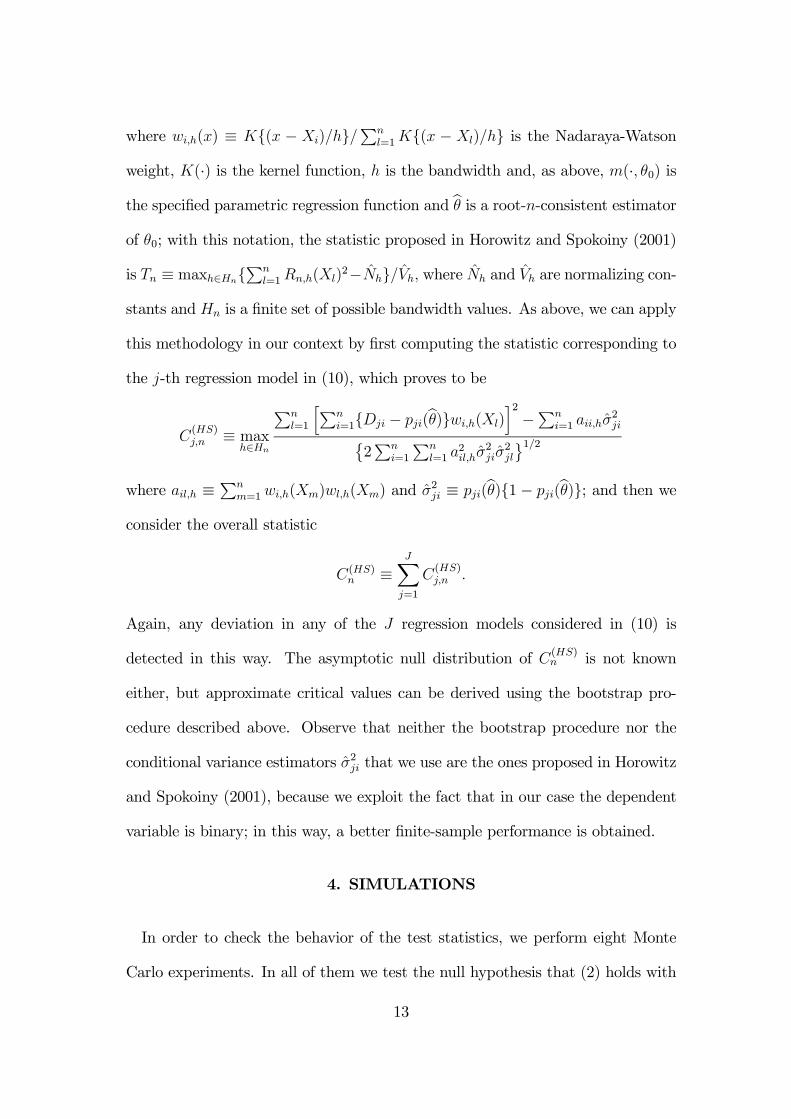
where wi,h(x) ≡ K{(x − Xi)/h}/Pn

l=1K{(x − Xl)/h} is the Nadaraya-Watson

weight, K(·) is the kernel function, h is the bandwidth and, as above, m(·, θ0) is

the specified parametric regression function and bθ is a root-n-consistent estimatorof θ0; with this notation, the statistic proposed in Horowitz and Spokoiny (2001)

is Tn ≡ maxh∈Hn{Pn

l=1Rn,h(Xl)2−Nh}/Vh, where Nh and Vh are normalizing con-

stants and Hn is a finite set of possible bandwidth values. As above, we can apply

this methodology in our context by first computing the statistic corresponding to

the j-th regression model in (10), which proves to be

C(HS)j,n ≡ max

h∈Hn

Pnl=1

hPni=1{Dji − pji(bθ)}wi,h(Xl)

i2−Pn

i=1 aii,hσ2ji©

2Pn

i=1

Pnl=1 a

2il,hσ

2jiσ

2jl

ª1/2where ail,h ≡

Pnm=1wi,h(Xm)wl,h(Xm) and σ2ji ≡ pji(bθ){1 − pji(bθ)}; and then we

consider the overall statistic

C(HS)n ≡

JXj=1

C(HS)j,n .

Again, any deviation in any of the J regression models considered in (10) is

detected in this way. The asymptotic null distribution of C(HS)n is not known

either, but approximate critical values can be derived using the bootstrap pro-

cedure described above. Observe that neither the bootstrap procedure nor the

conditional variance estimators σ2ji that we use are the ones proposed in Horowitz

and Spokoiny (2001), because we exploit the fact that in our case the dependent

variable is binary; in this way, a better finite-sample performance is obtained.

4. SIMULATIONS

In order to check the behavior of the test statistics, we perform eight Monte

Carlo experiments. In all of them we test the null hypothesis that (2) holds with

13

the standard normal distribution as F (·). With these experiments we seek to

examine whether the empirical size of the statistics is accurate, and also whether

the statistics detect misspecification in the latent regression model due to non-

linearities (Models 1-4), heteroskedasticity (Models 5-6) and non-normality in the

distribution function F (·) (Models 7-8). In four experiments (Models 1, 3, 5, 7)

the dependent variable Y only has two possible values (i.e. J = 1); in the other

four Y has three possible values (i.e. J = 2). In six experiments (Models 1-2 and

5-8) only two regressors are included: a constant variable and a normal one; in

the other two, an additional regressor is included in order to examine the extent

to which results change if the number of regressors increases.

The specific models that we consider are as follows:

• Model 1 : We generate n i.i.d. random vectors {(X2i, ui)0}ni=1, where X2i and

ui are independent with standard normal distribution; then Y ∗i = X0iβ0 +

c(X22i − 1) + ui, where Xi = (1,X2i)

0, β0 = (0, 1)0 and the value of c varies;

finally Yi = 0 if Y ∗i < 0, or 1 if Y ∗i ≥ 0.

• Model 2 : {(X2i, ui)0}ni=1 are generated as in Model 1; then Y ∗i = X

0iβ0 +

c(X22i − 1) + ui, where Xi = (1,X2i)

0, β0 = (1, 1)0 and the value of c varies;

finally Yi = 0 if Y ∗i < 0, or 1 if 0 ≤ Y ∗i < µ0, or 2 if Y∗i ≥ µ0, where µ0 = 2.

• Model 3 : We generate n i.i.d. random vectors {(X2i, X3i, ui)0}ni=1 all indepen-

dent with standard normal distribution; then Y ∗i = X0iβ0+ c(X2

1i−1)(X22i−

1) + ui, where Xi = (1, X2i,X3i)0, β0 = (0, 1, 1)

0 and the value of c varies;

finally Yi = 0 if Y ∗i < 0, or 1 if Y ∗i ≥ 0.

• Model 4 : {(X2i, X3i, ui)0}ni=1 are generated as in Model 3; then Y ∗i = X

0iβ0+

c(X21i − 1)(X2

2i − 1) + ui, where Xi = (1,X2i,X3i)0, β0 = (1, 1, 1)

0 and the

14

value of c varies; finally Yi = 0 if Y ∗i < 0, or 1 if 0 ≤ Y ∗i < µ0, or 2 if

Y ∗i ≥ µ0, where µ0 = 2.

• Model 5 : Data are generated as in Model 1 with c = 0, but now the condi-

tional distribution of ui givenX2i = x is normal with zero mean and variance

exp(dX2i − d2/2) for various d; hence, the unconditional distribution of ui

has zero mean and unit variance.

• Model 6 : Data are generated as in Model 2 with c = 0, but now ui is

generated as in Model 5.

• Model 7 : Data are generated as in Model 1 with c = 0, but now ui =

|d|1/2 εi− |d|−1/2 if d > 0, or ui = − |d|1/2 εi+ |d|−1/2 if d < 0, and εi follows a

gamma distribution with density function fε(x) = x(1/|d|)−1 exp(−x)/Γ(1/ |d|)

for various d; hence ui has zero mean and unit variance. The limit distrib-

ution of ui as d approaches 0 is the standard normal one, but if |d| is large

the distribution of ui is highly skewed (for d = 0, we generate ui from a

standard normal distribution).

• Model 8 : Data are generated as in Model 2 with c = 0, but now ui is

generated as in Model 7.

In all cases parameters are estimated by maximum likelihood assuming that

the null hypothesis holds. Note that in Models 1-4 H0 is true if and only if

c = 0, whereas in Models 5-8 H0 is true if and only if d = 0. In Tables 1-8 we

report the proportions of rejections of H0 at the 5% significance level for two

different sample sizes: n = 100 and n = 500. When a bootstrap procedure is

required we use B = 100 bootstrap replications. All results are based on 1000

15

simulation runs, performed using GAUSS programmes that are available from

the authors on request. When computing C(MP )n,l we consider various possible

partitions of the support, but we only report the results for the statistic that

yields the best performance, namely, C(MP )n,3 with G = 2 and A1 = R×(−∞, 0)

in Models 1-2 and 5-8; and C(MP )n,3 with G = 4 and A1 = R×(−∞, 0)× (−∞, 0),

A2 = R×(−∞, 0) × [0,∞), A3 = R×[0,∞) × (−∞, 0) in Models 3-4. When

computing C(HS)n we use a Gaussian kernel and, after some preliminary results,

we decide to choose Hn = { i2 , for i = 1, ..., 5} when n = 100 and Hn = { 3i10 , for

i = 1, ..., 5} when n = 500.

First we discuss the results that we obtain for the statistics based on conditional

moment restrictions. In all cases, the empirical size of the tests based on C(M)n,2

is much higher than the nominal level; this overrejection problem is especially

severe when n = 100, and leads us to disregard C(M)n,2 as a test statistic. When

we use C(M)n,1 the null hypothesis is also rejected too often; additionally, under the

alternative the power of C(M)n,1 is much lower than that obtained with the other

statistics. Therefore, the most reasonable moment-based statistic proves to be

C(M)n,3 , that is, it is crucial to take into account the specific nature of discrete choice

models when estimating the covariance matrix V0. Also observe that increasing

the degrees of freedom by partitioning the support of the independent variables

does not usually produce an increase in the power of the tests; the only exception

to this is when detecting non-normality (compare C(M)n,3 and C

(MP )n,3 in Table 8). On

the other hand, the test of overidentifying restrictions C(BC)n yields worse results

than the others, except again when detecting non-normal errors; in this case its

performance is comparable to (or even better than) that of the others.

As regards the statistics based on the comparison between parametric and non-

16

parametric estimations, all three behave reasonably well in terms of size. When

comparing power performance, statistic C(HS)n yields the best results in almost all

cases. This is not a surprise in Models 1, 3, 5, 7, since they are all regression mod-

els, and Horowitz and Spokoiny (2001) derive the optimality of their statistic in

this context; our results suggest that this optimality property also holds when it is

applied in general ordered discrete choice models. The only exception to this rule

is Model 8, where the generalization of Stute’s statistic yields somewhat better

results than C(HS)n . Comparing C(AN)

n and C(ST )n , the latter performs better when

testing the specification of a binary choice models, but when J ≥ 2 our results are

not so conclusive: Andrew’s statistic performs better than the generalization of

Stute’s statistic to detect non-linearities, but it performs worse with non-normal

errors.

Finally, if we compare the two statistics that perform best from each approach,

namely C(M)n,3 and C

(HS)n , there is no clear-cut answer to the question of which of

them performs better: the former performs better in detecting heteroskedasticity

in the latent regression model, whereas the latter performs better in detecting

non-normality or when the number of regressors is greater than one. Taking into

account the huge difference in computation time between them, one might be

tempted to say that C(M)n,3 should be preferred, but if computation time considera-

tions are disregarded, then our results show that the gain in power that is obtained

with the generalization of Horowitz-Spokoiny’s statistic is enough reward for the

additional programming effort.

17

5. EMPIRICAL APPLICATIONS

As an empirical illustration, we apply all the test statistics in two different

contexts. First, we consider the well-known data on extramarital affairs described

in Fair (1978). This is a famous data set that has become a milestone for models

with qualitative dependent variable. The data come from a survey published in

1969 in Psychology Today, with questions about characteristics of the individual

and the number of extramarital affairs (NEA) during the past year. The size

of the sample is 601. As a dependent variable we consider: Y = 0 if NEA=

0, Y = 1 if NEA= 1, 2, 3, or Y = 2 if NEA≥ 4. First we analyse whether

an ordered probit specification is adequate for the conditional distribution of Y

given as explanatory variables a constant variable, number of years married and

sex (0 for female, 1 for male). Then we repeat the analysis using all possible

explanatory variables, i.e. the three previous ones plus religiousness, education,

whether there are children or not, age and self rating of marriage. In Table

9 we report the results of the ML estimation and in Table 10 we report the

specification test statistics that are obtained. The statistic C(MP )n,3 is computed

with G = 2 and partitioning the support of the regressors according to sex; on

the other hand, the kernel weights required to obtain C(HS)n are computed using

a Gaussian kernel, regressors previously standardized to have unit variance, and

the family of bandwidths Hn = { 3i10, for i = 1, ..., 5}. In all cases the bootstrap

p-values are obtained with B = 1000 bootstrap replications. The results reported

in Table 10 suggest that the ordered probit specification might not be adequate

for Y | X when X only includes a constant variable, number of years married and

sex (the specification is rejected at the 10% level with most test statistics), but

18

there is no evidence against it when X includes all possible explanatory variables.

As a second example, we consider the determinants of women’s labour market

participation and the type of participation (work full-time or part-time). Liter-

ature has broadly dealt with this topic and its influence on fertility and divorce

rate, among other variables. We use data from the PSID (Wave 2001) to ex-

plain whether a woman does not work, works part-time or works full time. Our

sample contains 2866 observations; this sample has been obtained considering

only those women whose age is between 20 and 45, and whose marital status is

other than “never married”. Using information from the variable “Total hours

of work (wife)”, we define our dependent variable as follows: 0 if the woman re-

ports 0 hours, 1 if she reports a positive number of hours, but less than a certain

level φ, and 2 if the hours reported are greater than φ (specifically, we choose

φ = 1440 hours per year). We consider the following variables as determinants of

this employment status: age (as a proxy for experience), age square (to reflect the

non-linear influence of experience on employment status), whether the household

contains children or not, education and the husband’s labour income. In Table 10

we report the results of the ML estimation and the specification test statistics that

are obtained. The statistic C(MP )n,3 is computed with G = 2 and partitioning the

support of the regressors according to education (higher or lower than the mean

level), and C(HS)n is computed as in the previous application. Bootstrap p-values

are again obtained with B = 1000 bootstrap replications. The results reported in

Table 10 show that the ordered probit specification is rejected at the usual signif-

icance levels with almost all test statistics. However, if we consider a distribution

function F (·) with fatter tails (specifically, a Student’s t cdf with 5 degrees of

freedom, re-scaled to have unit variance), results change dramatically: this spec-

19

ification is not rejected at the 5% level with most test statistics. Moreover, an

adequate choice of F (·) is also crucial in analysing the influence of regressors on

employment status: note that estimations with a Student’s t cdf suggest that age,

rather than husband’s income, is the most significant explanatory variable.

6. CONCLUDING REMARKS

We discuss in this paper how to test the specification of ordered discrete choice

models. Two main approaches can be followed: tests based on conditional moment

restrictions and tests based on comparisons between parametric and nonparamet-

ric estimations. Our contribution in this paper is threefold: first, we propose a

variant of the usual conditional moment statistics that exploits all the information

in the model and is easy to compute (it is based on an artificial regression); sec-

ond, we propose generalizations of the test statistics proposed in Stute (1997) and

Horowitz and Spokoiny (2001), and describe how bootstrap critical values can be

obtained for them in our context; and third, we compare the performance of these

statistics (and some others) using various models that allow us to examine the em-

pirical size of the tests and their ability to detect deviations from the assumptions

that are usually made in applications: linearity, homoskedasticity and normality

in the latent regression model. Our simulation results show that the behaviour

of conditional moment tests crucially depends on how the covariance matrix is

estimated; furthermore, if this estimator is adequately chosen, the resulting test

statistic outperforms almost all other statistics considered here. On the other

hand, our simulation results suggest that the optimality property of Horowitz-

Spokoiny’s statistic in regression models may also hold for the generalization of

the statistic that we propose. Finally, the results of the empirical applications that

20

we include to illustrate the performance of the statistics highlight the importance

of selecting an accurate test statistic.

APPENDIX

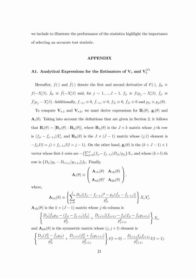
A1. Analytical Expressions for the Estimators of V0 and V(P )0

Hereafter, f(·) and f(·) denote the first and second derivative of F (·), f0i ≡

f(−X 0iβ), f0i ≡ f(−X 0

iβ) and, for j = 1, ..., J − 1, fji ≡ f(µj − X 0iβ), fji ≡

f(µj −X 0iβ). Additionally, f−1,i ≡ 0, f−1,i ≡ 0, fJi ≡ 0, fJi ≡ 0 and pji ≡ pji(θ).

To compute Vn,1 and Vn,2, we must derive expressions for Bi(θ), gi(θ) and

Ai(θ). Taking into account the definitions that are given in Section 2, it follows

that Bi(θ) = [B1i(θ) : B2i(θ)], where B1i(θ) is the J × k matrix whose j-th row

is (fji − fj−1,i)X0i, and B2i(θ) is the J × (J − 1) matrix whose (j, l) element is

−fjiI(l = j) + fj−1,iI(l = j − 1). On the other hand, gi(θ) is the (k + J − 1)× 1

vector whose first k rows are −{PJ

j=0(fji−fj−1,i)Dji/pji}Xi, and whose (k+ l)-th

row is {Dli/pli −Dl+1,i/pl+1,i}fli. Finally,

Ai(θ) ≡

⎛⎜⎝ A11i(θ) A12i(θ)

A12i(θ)0 A22i(θ)

⎞⎟⎠ ,

where,

A11i(θ) ≡(

JXj=0

Dji[(fji − fj−1,i)2 − pji(fji − fj−1,i)]

p2ji

)XiX

0i,

A12i(θ) is the k × (J − 1) matrix whose j-th column is(Dji[fjipji − (fji − fj−1,i)fji]

p2ji+

Dj+1,i[(fj+1,i − fji)fji − fjipj+1,i]

p2j+1,i

)Xi,

and A22i(θ) is the symmetric matrix whose (j, j + l) element is(Dji(f

2ji − fjipji)

p2ji+

Dj+1,i(f2ji + fjipj+1,i)

p2j+1,i

)I(l = 0)− Dj+1,ifjifj+1,i

p2j+1,iI(l = 1).

21

To compute Vn,3, we must derive expressions for EX{mi(θ)mi(θ)0}, EX{mi(θ)

gi(θ)0} and EX{gi(θ)gi(θ)0}. In this case EX{mi(θ)mi(θ)

0} is the J×J symmetric

matrix whose (j, j) element is pji(1 − pji) and whose (j, l) element, for l > j, is

−pjipli. On the other hand, EX{mi(θ)gi(θ)0} = −Bi(θ). Finally,

EX{gi(θ)gi(θ)0} ≡

⎛⎜⎝ A∗11i(θ) A∗12i(θ)

A∗12i(θ)0 A∗22i(θ)

⎞⎟⎠ ,

where A∗11i(θ) ≡ {PJ

j=0 (fji − fj−1,i)2 /pji}XiX

0i, A

∗12i(θ) is the k× (J −1) matrix

whose j-th column is {(fj+1,i− fji)/pj+1,i− (fji− fj−1,i)/pji}fjiXi, and A∗22i(θ) is

the symmetric matrix whose (j, l) element, for l ≥ j, is (1/pji + 1/pj+1,i)f2jiI(l =

j)− (fjifj+1,i/pj+1,i)I(l = j + 1).

As for the estimators of V(P )0 , note that V(P )

n,1 and V(P )n,2 can be computed using

the above expressions. To compute V(P )n,3 , observe that EX{m(P )

i (θ)m(P )i (θ)0} =

EX{mi(θ)mi(θ)0}⊗ (PiP

0i) and EX{m(P )

i (θ)gi(θ)0} = −B(P )i (θ).

A2. Artificial Regressions to Compute C(M)n,3 and C(MP )

n,3

Taking into account the expression for Vn,3, in order to derive an artificial

regression whose explained sum of squares is C(M)n,3 , first we use a Cholesky de-

composition of n−1Pn

i=1EX{mi(bθ)mi(bθ)0} to derive the first set of explanatoryvariables in the artificial regression, and then we define the remaining explanatory

variables and the dependent variable accordingly. Here we describe the artificial

regression that is obtained in this way.

Denote bpji ≡ pji(bθ) and bδji ≡ 1 − F (bµj − X 0ibβ) + F (−X 0

ibβ) and consider the

22

J × 1 vectors cji, dji, ei,, fji, whose l-th components are defined by:

cji,l ≡ {bpjiI(l < j) + bδj−1,iI(l = j)}/(bpjibδjibδj−1,i)1/2,dji,l ≡ bp1/2li [−bpjiI(l < j) + bδjiI(l = j)]/(bδlibδl−1,i)1/2,ei,l ≡ f(bµl −X 0

ibβ)− f(bµl−1 −X 0

ibβ),

fji,l ≡ f(bµj −X 0ibβ){I(l = j + 1)− I(l = j)}.

If we define Z ≡ [z01, ..., z0n]0, where zi is the J × 1 vector whose j-th element is

c0jimi, andW =[W(1) :W(2) :W(3)], whereW(l) ≡ [w(l)01 , ...,w

(l)0n ]0 for l = 1, 2, 3,

w(1)i is the J ×J matrix whose j-th column is dji, w

(2)i is the J × k matrix whose

j-th row is c0jieiX0i and w

(3)i is the J × (J − 1) matrix whose (j, l) element is c0jifli,

then it follows that Z0W(1) =Pn

i=1mi(bθ)0, Z0W∗= −Pn

i=1 gi(bθ)= 0, whereW∗ ≡

[W(2) :W(3)], andW(1)0W(1) −W(1)0W∗(W0∗W∗)

−1W0

∗W(1) =nVn,3. Therefore

C(M)n,3 coincides with the explained sum of squares in the artificial regression with

vector of dependent observations Z and matrix of observations W. Similarly,

C(MP )n,3 coincides with the explained sum of squares in the artificial regression with

vector of dependent observations Z(P ) ≡ [z(P )01 , ..., z(P )0n ]0 andmatrix of observations

W(P ) ≡ [W(P1) :W(P2) :W(P3)], where z(P )i ≡ zi ⊗Pi,W(Pl)=[w(Pl)01 , ...,w

(Pl)0n ]0

for l = 1, 2, 3, w(P1)i ≡ w(1)

i ⊗ (PiP0i), w

(P2)i ≡ w(2)

i ⊗Pi and w(P3)i ≡ w(3)

i ⊗Pi.

23

REFERENCES

Amemiya, T. (1985). Advanced Econometrics, Harvard University Press, Cam-

bridge.

Andrews, D. W. (1988). “Chi-Square Diagnostic Tests for Econometric Models”,

Journal of Econometrics, Vol. 37, pp. 135-156.

Andrews, D. W. (1997). “A Conditional Kolmogorov Test”, Econometrica, Vol.

65, pp. 1097-1128.

Butler, J. S. and Chatterjee, P. (1997). “Tests of the specification of univariate

and bivariate ordered probit”, Review of Economics and Statistics, Vol. 79, pp.

343-347.

Calhoun, C. A. (1989). “Estimating the Distribution of Desired Family Size and

Excess Fertility”, Journal of Human Resources, Vol. 24, pp. 709-724.

Glewwe, P. (1997). “A Test of the Normality Assumption in the Ordered Probit

Model”. Econometric Reviews, Vol. 16, pp. 1-19

Gustaffson, S. and Stafford, F. (1992). “Child Care Subsidies and Labor Supply

in Sweden”, Journal of Human Resources, Vol. 27, pp. 204-230.

Hamilton, J. (1994), Time Series Analysis, Princeton University Press, Princeton.

Horowitz, J. L. and Spokoiny, V. G. (2001). “An Adaptive, Rate-Optimal Test

of a Parametric Mean-Regression Model against a Nonparametric Alternative”,

Econometrica, Vol. 69, pp. 599-631.

24

Jiménez, E. and Kugler, B. (1987). “The Earnings Impact of Training Duration in

a Developing Country: An Ordered Probit Selection Model of Colombia’s Servicio

Nacional de Aprendizaje”, Journal of Human Resources, Vol. 22, pp. 228-247.

Klein, R.W. and Sherman, R.P. (1997). “Estimating New Product Demand from

Biased Survey Data”, Journal of Econometrics, Vol. 76, pp. 53-76.

Klein, R.W. and Sherman, R.P. (2002). “Shift Restrictions and Semiparametric

Estimation in Ordered Response Models”, Econometrica, Vol. 70, pp. 663-691.

MacKinnon, J. G. (1992). “Model Specification Tests and Artificial Regressions”,

Journal of Economic Literature, Vol. 30, pp. 102-146.

Matzkin, R. (1992). “Nonparametric and Distribution-Free Estimation of the

Binary Choice and the Threshold-Crossing Models”, Econometrica, Vol. 60, pp.

239-270.

Murphy, A. (1996). “Simple LM Tests of Mis-Specification for Ordered Logit

Models”, Economics Letters, Vol. 52, pp. 137-141.

Newey, W. K. (1985). “Maximum Likelihood Specification Testing and Condi-

tional Moment Tests”, Econometrica, Vol. 53, pp. 1047-1070.

Santos Silva, J. M. C. (2001). “A Score Test for Non-Nested Hypotheses with

Applications to Discrete Data Models”, Journal of Applied Econometrics, Vol.

16, pp. 577-597.

Stute, W. (1997). “Nonparametric Model Checks for Regression”, Annals of Sta-

tistics, Vol. 25, pp. 613-641.

25

Stute, W., González-Manteiga, W. and Presedo-Quindimil, M. (1998). “Boot-

strap Approximations in Model Checks for Regression”, Journal of the American

Statistical Association, Vol. 93, pp. 141-149.

Tauchen, G. E. (1985). “Diagnostic Testing and Evaluation of Maximum Likeli-

hood Models”, Journal of Econometrics, Vol. 30, pp. 415-443.

Weiss, A. A. (1997). “Specification Tests in Ordered Logit and Probit Models”,

Econometric Reviews, Vol. 16, pp. 361-391.

26

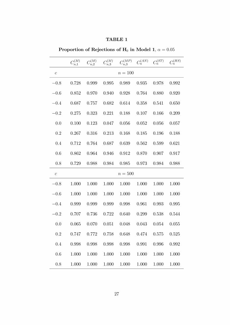
TABLE 1

Proportion of Rejections of H0 in Model 1, α = 0.05

C(M)n,1 C

(M)n,2 C

(M)n,3 C

(MP )n,3 C

(AN)n C

(ST )n C

(HS)n

c n = 100

−0.8 0.728 0.999 0.995 0.989 0.935 0.978 0.992

−0.6 0.852 0.970 0.940 0.928 0.764 0.880 0.920

−0.4 0.687 0.757 0.682 0.614 0.358 0.541 0.650

−0.2 0.275 0.323 0.221 0.188 0.107 0.166 0.209

0.0 0.100 0.123 0.047 0.056 0.052 0.056 0.057

0.2 0.267 0.316 0.213 0.168 0.185 0.196 0.188

0.4 0.712 0.764 0.687 0.639 0.562 0.599 0.621

0.6 0.862 0.964 0.946 0.912 0.870 0.907 0.917

0.8 0.729 0.988 0.984 0.985 0.973 0.984 0.988

c n = 500

−0.8 1.000 1.000 1.000 1.000 1.000 1.000 1.000

−0.6 1.000 1.000 1.000 1.000 1.000 1.000 1.000

−0.4 0.999 0.999 0.999 0.998 0.961 0.993 0.995

−0.2 0.707 0.736 0.722 0.640 0.299 0.538 0.544

0.0 0.065 0.070 0.051 0.048 0.043 0.054 0.055

0.2 0.747 0.772 0.758 0.648 0.474 0.575 0.525

0.4 0.998 0.998 0.998 0.998 0.991 0.996 0.992

0.6 1.000 1.000 1.000 1.000 1.000 1.000 1.000

0.8 1.000 1.000 1.000 1.000 1.000 1.000 1.000

27

TABLE 2


C(M)n,1 C

(M)n,2 C

(M)n,3 C

(MP )n,3 C

(BC)n C

(AN)n C

(ST )n C

(HS)n

c n = 100

−0.8 0.290 0.994 0.987 0.996 0.580 0.970 0.741 0.980

−0.6 0.321 0.935 0.933 0.939 0.637 0.907 0.671 0.917

−0.4 0.253 0.735 0.721 0.704 0.555 0.663 0.542 0.721

−0.2 0.118 0.330 0.272 0.253 0.217 0.238 0.226 0.293

0.0 0.067 0.120 0.048 0.044 0.072 0.069 0.049 0.060

0.2 0.097 0.302 0.252 0.233 0.340 0.207 0.189 0.240

0.4 0.242 0.737 0.729 0.725 0.696 0.621 0.440 0.702

0.6 0.297 0.935 0.935 0.950 0.754 0.896 0.716 0.918

0.8 0.252 0.990 0.986 0.995 0.674 0.983 0.871 0.986

c n = 500

−0.8 0.999 1.000 1.000 1.000 0.999 1.000 1.000 1.000

−0.6 0.998 1.000 1.000 1.000 1.000 1.000 1.000 1.000

−0.4 0.976 0.996 0.997 1.000 1.000 1.000 0.997 1.000

−0.2 0.703 0.860 0.858 0.874 0.831 0.784 0.729 0.843

0.0 0.064 0.079 0.050 0.053 0.052 0.045 0.060 0.052

0.2 0.718 0.856 0.875 0.893 0.859 0.745 0.621 0.811

0.4 0.989 0.999 1.000 1.000 0.999 0.999 0.998 1.000

0.6 1.000 1.000 1.000 1.000 1.000 1.000 1.000 1.000

0.8 1.000 1.000 1.000 1.000 0.998 1.000 1.000 1.000

28

TABLE 3


C(M)n,1 C

(M)n,2 C

(M)n,3 C

(MP )n,3 C

(AN)n C

(ST )n C

(HS)n

c n = 100

−0.8 0.533 0.606 0.561 0.561 0.467 0.640 0.852

−0.6 0.480 0.558 0.497 0.468 0.330 0.428 0.656

−0.4 0.324 0.441 0.307 0.272 0.188 0.217 0.358

−0.2 0.185 0.261 0.126 0.093 0.085 0.079 0.144

0.0 0.109 0.170 0.052 0.054 0.057 0.061 0.066

0.2 0.170 0.247 0.105 0.099 0.087 0.103 0.168

0.4 0.338 0.453 0.322 0.285 0.107 0.154 0.402

0.6 0.476 0.550 0.469 0.454 0.179 0.276 0.661

0.8 0.500 0.569 0.536 0.539 0.248 0.402 0.856

c n = 500

−0.8 0.505 0.615 0.832 0.981 0.995 1.000 1.000

−0.6 0.430 0.519 0.752 0.941 0.958 0.992 1.000

−0.4 0.476 0.496 0.617 0.743 0.693 0.800 0.960

−0.2 0.324 0.366 0.340 0.263 0.197 0.206 0.394

0.0 0.062 0.072 0.050 0.048 0.067 0.059 0.072

0.2 0.298 0.329 0.291 0.239 0.116 0.156 0.390

0.4 0.457 0.475 0.598 0.720 0.394 0.560 0.953

0.6 0.426 0.482 0.726 0.927 0.751 0.948 1.000

0.8 0.498 0.590 0.815 0.978 0.950 0.998 1.000

29

TABLE 4


C(M)n,1 C

(M)n,2 C

(M)n,3 C

(MP )n,3 C

(BC)n C

(AN)n C

(ST )n C

(HS)n

c n = 100

−0.8 0.280 0.526 0.393 0.373 0.350 0.510 0.334 0.739

−0.6 0.251 0.505 0.388 0.303 0.400 0.374 0.257 0.551

−0.4 0.216 0.437 0.311 0.248 0.350 0.218 0.157 0.302

−0.2 0.137 0.284 0.154 0.123 0.215 0.110 0.092 0.107

0.0 0.109 0.214 0.054 0.053 0.102 0.050 0.065 0.047

0.2 0.142 0.288 0.156 0.143 0.113 0.082 0.104 0.212

0.4 0.215 0.434 0.302 0.231 0.171 0.147 0.185 0.496

0.6 0.252 0.522 0.387 0.318 0.234 0.180 0.251 0.670

0.8 0.269 0.531 0.428 0.401 0.204 0.241 0.246 0.766

c n = 500

−0.8 0.606 0.812 0.862 0.962 0.906 1.000 0.999 1.000

−0.6 0.569 0.699 0.819 0.883 0.920 0.997 0.981 0.999

−0.4 0.520 0.601 0.732 0.703 0.858 0.847 0.764 0.973

−0.2 0.319 0.422 0.437 0.302 0.451 0.299 0.252 0.384

0.0 0.081 0.098 0.047 0.055 0.050 0.062 0.051 0.060

0.2 0.308 0.407 0.422 0.286 0.283 0.196 0.230 0.676

0.4 0.543 0.622 0.743 0.697 0.734 0.582 0.630 0.995

0.6 0.547 0.675 0.820 0.864 0.855 0.835 0.803 1.000

0.8 0.585 0.763 0.844 0.951 0.830 0.957 0.871 1.000

30

TABLE 5


C(M)n,1 C

(M)n,2 C

(M)n,3 C

(MP )n,3 C

(AN)n C

(ST )n C

(HS)n

d n = 100

−0.8 0.564 0.613 0.479 0.383 0.356 0.395 0.406

−0.6 0.382 0.438 0.318 0.251 0.231 0.243 0.252

−0.4 0.223 0.266 0.165 0.135 0.138 0.147 0.155

−0.2 0.143 0.169 0.083 0.075 0.080 0.074 0.074

0.0 0.100 0.123 0.047 0.056 0.052 0.056 0.057

0.2 0.124 0.163 0.065 0.057 0.066 0.074 0.083

0.4 0.240 0.285 0.181 0.130 0.087 0.145 0.158

0.6 0.397 0.443 0.315 0.253 0.130 0.225 0.275

0.8 0.535 0.597 0.460 0.371 0.204 0.355 0.424

d n = 500

−0.8 0.988 0.990 0.988 0.975 0.918 0.957 0.942

−0.6 0.930 0.936 0.924 0.868 0.711 0.815 0.756

−0.4 0.663 0.686 0.657 0.539 0.371 0.486 0.413

−0.2 0.251 0.266 0.227 0.182 0.127 0.151 0.133

0.0 0.065 0.070 0.051 0.048 0.043 0.054 0.055

0.2 0.231 0.248 0.217 0.154 0.086 0.156 0.149

0.4 0.649 0.666 0.652 0.530 0.238 0.455 0.438

0.6 0.917 0.926 0.913 0.865 0.508 0.768 0.763

0.8 0.988 0.993 0.988 0.980 0.775 0.945 0.954

31

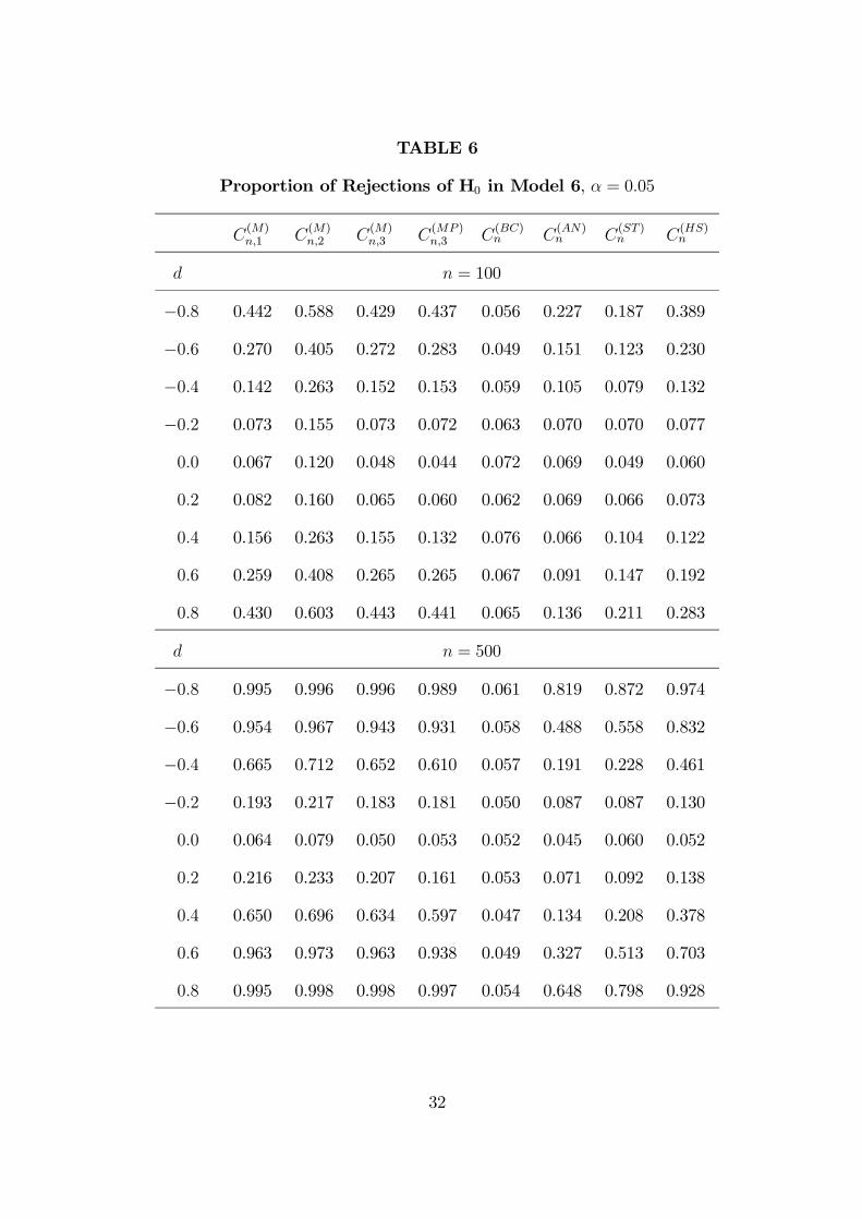
TABLE 6


C(M)n,1 C

(M)n,2 C

(M)n,3 C

(MP )n,3 C

(BC)n C

(AN)n C

(ST )n C

(HS)n

d n = 100

−0.8 0.442 0.588 0.429 0.437 0.056 0.227 0.187 0.389

−0.6 0.270 0.405 0.272 0.283 0.049 0.151 0.123 0.230

−0.4 0.142 0.263 0.152 0.153 0.059 0.105 0.079 0.132

−0.2 0.073 0.155 0.073 0.072 0.063 0.070 0.070 0.077

0.0 0.067 0.120 0.048 0.044 0.072 0.069 0.049 0.060

0.2 0.082 0.160 0.065 0.060 0.062 0.069 0.066 0.073

0.4 0.156 0.263 0.155 0.132 0.076 0.066 0.104 0.122

0.6 0.259 0.408 0.265 0.265 0.067 0.091 0.147 0.192

0.8 0.430 0.603 0.443 0.441 0.065 0.136 0.211 0.283

d n = 500

−0.8 0.995 0.996 0.996 0.989 0.061 0.819 0.872 0.974

−0.6 0.954 0.967 0.943 0.931 0.058 0.488 0.558 0.832

−0.4 0.665 0.712 0.652 0.610 0.057 0.191 0.228 0.461

−0.2 0.193 0.217 0.183 0.181 0.050 0.087 0.087 0.130

0.0 0.064 0.079 0.050 0.053 0.052 0.045 0.060 0.052

0.2 0.216 0.233 0.207 0.161 0.053 0.071 0.092 0.138

0.4 0.650 0.696 0.634 0.597 0.047 0.134 0.208 0.378

0.6 0.963 0.973 0.963 0.938 0.049 0.327 0.513 0.703

0.8 0.995 0.998 0.998 0.997 0.054 0.648 0.798 0.928

32

TABLE 7


C(M)n,1 C

(M)n,2 C

(M)n,3 C

(MP )n,3 C

(AN)n C

(ST )n C

(HS)n

d n = 100

−0.8 0.486 0.550 0.308 0.254 0.142 0.287 0.342

−0.6 0.400 0.450 0.244 0.187 0.103 0.207 0.232

−0.4 0.273 0.337 0.185 0.118 0.086 0.164 0.181

−0.2 0.182 0.218 0.097 0.090 0.064 0.104 0.114

0.0 0.100 0.123 0.047 0.056 0.052 0.056 0.057

0.2 0.175 0.209 0.085 0.088 0.094 0.094 0.100

0.4 0.287 0.335 0.166 0.125 0.148 0.166 0.161

0.6 0.397 0.469 0.210 0.184 0.231 0.246 0.263

0.8 0.503 0.564 0.324 0.217 0.273 0.299 0.310

d n = 500

−0.8 0.985 0.991 0.970 0.950 0.682 0.943 0.930

−0.6 0.948 0.953 0.899 0.834 0.508 0.820 0.796

−0.4 0.831 0.850 0.768 0.658 0.345 0.605 0.555

−0.2 0.495 0.513 0.420 0.347 0.163 0.333 0.294

0.0 0.065 0.070 0.051 0.048 0.043 0.054 0.055

0.2 0.488 0.515 0.418 0.335 0.251 0.347 0.303

0.4 0.799 0.820 0.726 0.648 0.495 0.616 0.567

0.6 0.961 0.968 0.925 0.837 0.732 0.836 0.799

0.8 0.985 0.990 0.966 0.947 0.880 0.939 0.928

33

TABLE 8


C(M)n,1 C

(M)n,2 C

(M)n,3 C

(MP )n,3 C

(BC)n C

(AN)n C

(ST )n C

(HS)n

d n = 100

−0.8 0.350 0.601 0.393 0.492 0.515 0.388 0.668 0.589

−0.6 0.256 0.444 0.274 0.395 0.488 0.307 0.534 0.478

−0.4 0.198 0.354 0.233 0.256 0.359 0.196 0.412 0.316

−0.2 0.096 0.218 0.104 0.159 0.218 0.129 0.266 0.208

0.0 0.067 0.120 0.048 0.044 0.062 0.069 0.049 0.060

0.2 0.109 0.210 0.111 0.137 0.120 0.147 0.230 0.200

0.4 0.172 0.332 0.175 0.274 0.251 0.266 0.393 0.351

0.6 0.258 0.483 0.280 0.408 0.331 0.361 0.546 0.494

0.8 0.346 0.597 0.390 0.505 0.369 0.459 0.646 0.576

d n = 500

−0.8 0.899 0.974 0.964 1.000 0.984 0.993 1.000 0.999

−0.6 0.777 0.886 0.870 0.994 0.960 0.962 0.998 0.996

−0.4 0.589 0.739 0.710 0.945 0.900 0.808 0.946 0.937

−0.2 0.292 0.374 0.313 0.655 0.638 0.483 0.815 0.617

0.0 0.064 0.079 0.050 0.053 0.052 0.045 0.060 0.052

0.2 0.321 0.399 0.358 0.634 0.572 0.489 0.754 0.580

0.4 0.592 0.722 0.686 0.944 0.826 0.869 0.978 0.920

0.6 0.786 0.914 0.891 0.997 0.936 0.971 0.998 0.989

0.8 0.903 0.969 0.958 1.000 0.980 0.999 1.000 0.998

34

TABLE 9: Extramarital Affairs Data

Ordered Probit Model for Y | X

X = (X1, X2, X3) X = (X1, ...,X8)

Estimates (with t-statistics)

Constant −1.060(−9.077)

0.720(1.466)

Years of Marr. 0.040(3.976)

0.062(3.397)

Sex 0.096(0.883)

0.133(1.068)

Religiousness −0.202(−4.045)

Education 0.021(0.813)

Child./No Child. 0.149(0.942)

Age −0.235(−2.342)

S.R.M. −0.276(−5.426)

P-values of test statistics

C(M)n,1 0.307 0.421

C(M)n,2 0.063 0.372

C(M)n,3 0.076 0.365

C(MP )n,3 0.074 0.361

C(BC)n 0.082 0.134

C(AN)n 0.188 0.109

C(ST )n 0.115 0.348

C(HS)n 0.154 0.435

35

TABLE 10: Female Labour Participation Data

Ordered Discrete Choice Model for Y | X

Normal cdf Student’s t5 cdf

Estimates (with t-statistics)

Constant −0.553(−0.839)

−0.751(−1.163)

Age 0.054(1.253)

0.067(1.715)

Age2 −0.004(−0.586)

−0.008(−11.642)

Child./No Child. −0.226(−8.176)

−0.181(−8.780)

Education 0.074(6.515)

0.059(6.707)

Husband’s Income −0.009(−10.103)

−0.001(−1.140)

P-values of test statistics

C(M)n,1 0.002 0.227

C(M)n,2 0.001 0.215

C(M)n,3 0.001 0.173

C(MP )n,3 0.003 0.268

C(BC)n 0.002 0.010

C(AN)n 0.002 0.009

C(ST )n 0.125 0.121

C(HS)n 0.013 0.148

36

consistent specification tests for ordered discrete …

Documents