constrained efficiency in the neoclassical growth model with
TRANSCRIPT
Submitted to Econometrica
CONSTRAINED EFFICIENCY IN THE NEOCLASSICAL GROWTHMODEL WITH UNINSURABLE IDIOSYNCRATIC SHOCKS1
Julio Davila, Jay H. Hong, Per Krusell2,3 and Jose-Vıctor
Rıos-Rull4
We investigate the welfare properties of the one-sector neoclassical growth modelwith uninsurable idiosyncratic shocks. We focus on the notion of constrained effi-ciency used in the general equilibrium literature. Our characterization of constrainedefficiency uses the first-order condition of a constrained planner’s problem. This con-dition highlights the margins of relevance for whether capital is too high or too low:the factor composition of income of the (consumption-)poor. Using three calibrationscommonly considered in the literature, we illustrate that there can be either over-or underaccumulation of capital in steady state and that the constrained optimummay or may not be consistent with a nondegenerate long-run distribution of wealth.For the calibration that roughly matches the income and wealth distribution, theconstrained inefficiency of the market outcome is rather striking: it has much too lowa steady-state capital stock.
Keywords: Constrained Efficiency, Uninsurable Shocks.
1. INTRODUCTION
In this paper we investigate the welfare properties of the one-sector neoclassicalgrowth model with uninsurable idiosyncratic shocks but precautionary savings.This kind of model was originally developed and analyzed by Bewley (1986),Imrohoroglu (1989), Huggett (1993), and Aiyagari (1994), and it has becomea standard workhorse for quantitatively based theoretical analysis of macroeco-nomics and inequality. The framework is mostly used for positive analysis, but inthis paper we focus on some of its normative properties. In particular, we studythe constrained efficiency of the market allocations. We define this concept fol-lowing Diamond (1967), who in a similar context was interested in a notion ofefficiency that did not allow the planner to directly overcome the friction im-plied by missing markets. Constrained inefficiency is sometimes also thought ofin terms of a “pecuniary externality”: the incomplete market structure itself in-duces outcomes that could be improved on, in the Pareto sense, if consumers
Davila: Center for Operations Research and Econometrics, Universite c. de Louvain, Bel-gium and Paris School of Economics, Centre d’Economie de la Sorbonne-CNRS, [email protected]
Hong: University of Rochester. [email protected]: IIES, CAERP, CEPR, [email protected]ıos-Rull: University of Minnesota, Federal Reserve Bank of Minneapolis, CAERP, CEPR,
NBER. [email protected] thank Tim Kehoe, Michael Magill, Ivan Werning, and Martine Quinzii, as well as the
editor and three anonymous referees, for very helpful comments.2Corresponding author.3Krusell thanks the National Science Foundation.4Rıos-Rull thanks the National Science Foundation and the University of Pennsylvania
Research Foundation for support. The views expressed herein are those of the authors and notnecessarily those of the Federal Reserve Bank of Minneapolis or the Federal Reserve System.
1

2 DAVILA ET AL.
merely acted differently, i.e., if they used the same set of markets but departedfrom purely self-interested optimization.We find that the laissez-faire equilibrium generally is not constrained efficient
in our economy. In the baseline model, the key decision consumers make is howmuch to save, and the amount of savings influences equilibrium prices: the returnto capital and the wage. Furthermore, prices influence how the market incom-pleteness affects consumers. With shocks to individual wages or employment, alower wage and a higher rental rate make the uninsurable part of income smaller,suggesting that lower economy-wide saving may be welfare improving. Indeed, fora two-period economy we show that the laissez-faire equilibrium unambiguouslyhas too much savings: if consumers just saved a little less, they would all face lessuninsurable risk and all be better off. However, we also show that in economieswith longer lives, an effect appears that works in the opposite direction. Id-iosyncratic wage shocks generate wealth inequality, which propagates over time.Thus, since higher aggregate savings lower the return to wealth, an increase insavings can improve consumer welfare by reducing the wealth inequality inducedby missing insurance markets.A central part of the paper involves characterizing the precise conditions under
which there is oversaving and undersaving. We pay particular attention to theinfinite horizon version of our economy. We study the properties of constrained-optimal steady states and compare them to the laissez-faire outcomes. The anal-ysis is based on a functional first-order condition that is a necessary condition ofthe constrained-efficiency planning problem. This first-order condition is, to ourknowledge, new, and it is one of the key analytical tools put forth in this paper.Our central finding is that whether there is over- or underaccumulation of
capital depends very importantly on the factor composition of the income of thepoor agents. A key factor behind whether the constrained optimum should havehigher or lower capital than the laissez-faire equilibrium is the factor incomeof the (consumption-)poor, since these agents have a high weight due to theincompleteness of consumption insurance. One can show that the comparisonbetween their relative labor income and their relative asset income guides howthey are affected: if the poorest do better relative to the average for labor incomethan for asset income, then they are helped with a larger aggregate capitalstock. If instead the consumption-poor agents have an income composition thatis relatively stronger for assets than for labor income, the reverse result holds.In conclusion, in economies where the unlucky consumers do relatively better interms of their labor income, there is too little aggregate capital accumulation.We illustrate these properties quantitatively using a numerical model solu-
tion, where transition dynamics is taken into account. We study three cases:three commonly used versions of the standard model, each with a standard cal-ibration. The first case we look at—the “unemployment economy”—is based onunemployment shocks, as in the version of Krusell and Smith (1998) with homo-geneous preferences. For this economy, which has limited wealth dispersion, wefind a modest amount of capital overaccumulation, as in the simplest version of

CONSTRAINED EFFICIENCY 3
the two-period model we study.
The second and third calibrations feature underaccumulation of capital. Oneof them uses a calibration like that in Castaneda, Dıaz-Gimenez, and Rıos-Rull(1998). This setup has realistic wealth dispersion due to large and persistent,though strongly mean-reverting, labor income shocks. Here, the consumption-poor are mainly wealth-poor, and hence the planner should increase the capitalstock. Moreover, the discrepancy between the laissez-faire equilibrium and theconstrained optimum is large. In the third calibration, the calibration used inAiyagari (1994), the constrained-efficient steady state is only asymptotic: it in-volves ever-increasing wealth inequality, i.e., the underaccumulation is mainlycounteracted by making the rich save more and more.
Diamond (1967) first raised the possibility of constrained inefficiency in a one-period, one-good stock market economy with multiplicative uncertainty concern-ing production, but he actually found constrained efficiency for the particulareconomy under study. However, examples of constrained inefficiency of com-petitive equilibria were soon provided in Hart (1975), Diamond (1980), Stiglitz(1982), Loong and Zeckhauser (1982), Newbery and Stiglitz (1984), and Green-wald and Stiglitz (1986). In particular, Stiglitz (1982) established that the con-strained efficiency result shown in Diamond (1967) depended on his one-goodassumption; with more goods, a reallocation of investments and portfolios wouldin general influence relative prices and, given the incompleteness of markets,could also improve consumer welfare. Geanakoplos, Magill, Quinzii, and Dreze(1990) later established generic (in terms of initial endowments) constrained in-efficiency of competitive equilibria of a two-period stock market economy withmany goods.1 In contrast with the general equilibrium literature, we address theconstrained inefficiency issue in the infinite-horizon workhorse macroeconomicmodel with uninsurable idiosyncratic shocks.2 In our context, generic constrainedinefficiency also comes through relative prices, though across production inputsrather than across consumption goods. Our examples moreover demonstrate thatthe inefficiency can be quite drastic quantitatively (for plausible model calibra-tions) as well as, we think, intuitively easily understood.
Section 2 describes the two-period model and analyzes constrained efficiencyin this economy. It describes two cases: one without initial wealth heterogeneity,i.e., in the first period all consumers are identical, and one with initial wealthheterogeneity. The second of these cases is our way of illustrating how multi-period models, where wealth heterogeneity would be endogenous, would allownot only capital overaccumulation but also capital underaccumulation. Section 3describes the model with an infinite horizon and describes laissez-faire equilib-ria. The associated constrained-efficiency planning problem is then described inSection 4 and the central first-order condition is derived. Section 5 carries out
1In Geanakoplos and Polemarchakis (1986) this result is established for an exchange econ-omy. In that case the result is generic in initial endowments and utility functions.
2 For a study of uninsurable idiosyncratic shocks from an incomplete markets, general equi-librium perspective, see Carvajal and Polemarchakis (2011).
4 DAVILA ET AL.
the quantitative analysis for our different example calibrations of the infinite-horizon model. Before concluding in Section 7, Section 6 looks at two relevantextensions: a model with a labor-leisure choice and a model with “expenditureshocks” that do not involve relative prices. We discuss implementation, throughexplicit tax-transfer schemes, of the constrained optimum throughout the paper:in our two-period model, in Section 4.2, and in the quantitative section.
2. THE MECHANISMS: ILLUSTRATION USING A TWO-PERIOD MODEL
In the present section, we consider a two-period general equilibrium model ofprecautionary savings—a two-period version of Aiyagari (1994)—and use it tointroduce and illustrate the notion of constrained inefficiency. With the simplemodel we are able to establish some useful qualitative results and to discusssome features of the model that will later be of quantitative importance in ournumerically computed economies. We begin with an economy where consumersare identical in the first period (Section 2.1) and then consider initial wealthinequality (Section 2.2). Initial wealth heterogeneity is relevant since it will ariseendogenously in a multiperiod setting, where the nature of inequality—whetherit primarily reflects inequality in capital or labor income—turns out to be crucialfor the qualitative as well as quantitative results. Much later in the paper (Section6), we then revisit the two-period model for a brief discussion of two relevantextensions.
2.1. Ex ante identical consumers
Consider an economy with a continuum (measure 1) of two-period-lived, exante identical consumers. The consumers have time-additive, von Neumann-Morgenstern utility functions with a twice continuously differentiable, strictlyincreasing, and strictly concave period utility function u satisfying INADA con-ditions and a discount factor β. In the first period, period 1, each agent is en-dowed with ω units of output, which can be either consumed, c, or invested inan asset, a: capital. In period 2, consumers receive income from the capital theysaved in period 1 and from working. The labor income of any given individualis random. In particular, the labor endowment can be either high or low, and itis independent across agents. We denote the period 2 labor endowments e1 ande2, with 0 < e1 < e2; the probability that any agent’s labor endowment is e1 isπ. Due to the independence of shocks across consumers, a law of large numbersoperates so that also the fraction of agents with ei is πi; we sometimes use π todenote π1. That is, there is no uncertainty about the period 2 labor endowment:the supply of labor is constant at L = πe1 + (1− π)e2.In the second period, output comes from production using capital and labor
and a constant returns to scale (CRS) neoclassical production function f . Sinceall agents face the same maximization problem, and since this is a problem with astrictly concave objective and a linear constraint set, they will all make identical
CONSTRAINED EFFICIENCY 5
choices. Let the implied equilibrium choice of capital be K (per consumer, andin the aggregate, so that a = K). Then the output in period 2 is known to bef(K,L). Output is produced by perfectly competitive firms in our equilibrium:they sell the output to consumers and rent the capital and the labor servicesfrom the same consumers at rates r and w, respectively. In equilibrium, thus,r and w will be set to equal the marginal products of the inputs; in particular,they will be deterministic. This means that in period 1, each consumer will seehis capital income in period 2 as deterministic and equal to rK, whereas hislabor income is random and equal to we.It is a maintained assumption in our analysis that consumers can only save
using capital; in particular, there is no pure insurance instrument available forreducing the idiosyncratic risk, so the only way of influencing the risk is through“precautionary savings.”Given the above, we have
Definition 1. A competitive equilibrium is a vector (K, r,w) such that (i) Ksolves
maxa∈[−we1/r,ω]
u(ω − a) + β (πu(ra+ we1) + (1− π)u(ra+ we2))
and (ii) r = fk(K,L) and w = fl(K,L), with L = πe1 + (1− π)e2.
It is straightforward to show that an equilibrium with K ∈ (0, ω) exists undersuitable conditions on u and f .3
Can the market allocation be improved upon? The notion of constrained effi-ciency. In this economy, agents really make only one choice: the saving choice.Following the incomplete markets, general equilibrium literature, we discuss theefficiency properties of the equilibrium in terms of whether this one choice couldbe made in a better way: can it be made so as to improve on equilibrium util-ity? Formally, we call the equilibrium constrained efficient if there is no level ofsaving K such that, given competitive pricing of inputs in period 2, the utilityof the consumer is higher than under the competitive equilibrium. That is, theequilibrium (K, r,w) we consider is efficient if there is no K ∈ [0, ω] such that
u(ω−K)+β(πu(fk(K, L)K + fl(K, L)e1) + (1− π)u(fk(K, L)K + fl(K, L)e2)
)>
u(ω−K)+β (πu(fk(K,L)K + fl(K,L)e1) + (1− π)u(fk(K,L)K + fl(K,L)e2)) .
The question, thus, is whether a fictitious planner can improve on the al-location by simply commanding a different savings level for the representativeconsumer, while respecting all budget constraints of agents and letting firms op-erate freely under perfect competition. In particular, the fictitious planner is not
3In this section, we do not restrict borrowing unnecessarily; the consumer is allowed toborrow any amount as long as the debt can be paid back in all states of the world. Given thatthe utility function satisfies the INADA condition, we omit these issues in the present section.

6 DAVILA ET AL.
allowed to “complete the markets” or in any way transfer goods between luckyand unlucky consumers: the only insurance asset is still capital. Thus, at leastqualitatively, constrained inefficiency is a rather drastic form of market failure.The market outcome is constrained inefficient: the formal argument. In this
economy, whether or not it is possible to improve on the market allocation can beseen by considering the impact of a small variation dK of the aggregate capital.Differentiating the indirect utility, one obtains
dU = −u′(ω−K)dK+β (πu′(rK + we1)dC1 + (1− π)u′(rK + we2)dC2) ,
where dCi = rdK +Kdr + eidw, i ∈ 1, 2.The individual’s first-order condition for savings reads
u′(ω −K) = β (πu′(rK + we1) + (1− π)u′(rK + we2)) r.
This condition can be used to simplify the above expression, and it will leadmany of the effects of increasing capital to vanish. We thus obtain
dU = β
((πu′(rK + we1) + (1− π)u′(rK + we2))Kdr
+ (πu′(rK + we1)e1 + (1− π)u′(rK + we2)e2) dw
),
so that we see that any effect of a marginal change of savings away from thecompetitive equilibrium has to operate through its effect on factor prices. Thecancelations, of course, are just a result of the envelope theorem. As for howfactor prices are affected by capital, we note that dr = fKK(K,L)dK and dw =fKL(K,L)dK so that
dU = β
(πu′(rK + we1)(KfKK(K,L) + e1fKL(K,L))
+(1− π)u′(rK + we2)(KfKK(K,L) + e2fKL(K,L))
)dK.
Now note that because f is homogeneous of degree 1,KfKK(K,L)+LfKL(K,L) =0 and therefore
dU = β
(πu′(rK+we1)
(1− e1
L
)+(1−π)u′(rK+we2)
(1− e2
L
))fKKKdK.
Letting
χ ≡ u′(fk(K,L)k + fl(K,L)e1)
u′(fk(K,L)k + fl(K,L)2)> 1,
this can be rewritten as
dU = βu′(fk(K,L)k + fl(K,L)e2)π(χ− 1)(1− 1
L
)fkk(K,L)KdK.

CONSTRAINED EFFICIENCY 7
Thus, since fkk < 0, equilibrium utility increases if dK < 0. We conclude, moregenerally, that the equilibrium is constrained inefficient . As is clear from theanalysis, the key assumptions behind the result are that u is strictly concaveand that f has a strictly decreasing marginal product of capital.Specifically, as noted, the level of capital in the laissez-faire equilibrium is too
high: a higher utility is obtained if all consumers save a little less in period 1. Theintuitive reason for the overaccumulation of capital is as follows. More capitalsavings raises wages and lowers rental rates. The only source of market failure inthis economy is the incomplete insurance. A small decrease in K from the equi-librium level thus lowers w and raises r, thereby scaling down the part of theconsumer’s income that is stochastic and scaling up the part that is determin-istic: the amount of risk the consumer is exposed to is now smaller. Given thatthere is no direct insurance for this risk, this amounts to an improvement. The“distortion” on the agents’ savings by moving savings away from the competitiveequilibrium level for given prices is of a second-order magnitude, and thus themanipulation of prices so as to lower the de facto risk dominates.Market incompleteness is of course key to our finding of constrained ineffi-
ciency: unlike in the complete markets case, prices are not optimally set hereand agents’ influence on prices should therefore be taken into account whenmaking individual choices. An improvement on the competitive outcome thusrequires taking an aggregate, “planning” perspective.
2.2. The two-period model with initial wealth heterogeneity
We now let ω differ across individuals as the economy starts; let its distributionbe Γ. We will discuss the effects of altering total capital accumulation away fromthe laissez-faire level on consumers with different initial wealth holdings and thenpoint to how the two-period model with initial wealth heterogeneity can be usedto organize some of the findings for the quantitative infinite-horizon economystudied in the remainder of the paper.Equilibrium and effects of altering aggregate saving. For the new setting, we
have
Definition 2. A competitive equilibrium is a vector (a(ω),K, r, w) such that(i) a(ω) solves
maxa∈[0,ω]
u(ω − a) + β (πu(ra+ we1) + (1− π)u(ra+ we2)) ;
(ii) K =∫ωa(ω)Γ(dω); and (iii) r = fk(K,L) and w = fl(K,L), with L =
πe1 + (1− π)e2.
Does a decrease in capital accumulation—engineered, say, by making all agentssave ϵ > 0 less—increase utility here as well? Again, the key question is howthe resulting price change (an increase in r and a decrease in w) would affectconsumers’ utility. Here, unlike in the case where consumers are equal ex ante,

8 DAVILA ET AL.
this question does not have an unambiguous answer: different consumers havedifferent income compositions, and in particular those who are poor initially willrely more on labor income and therefore can be made worse off by a fall inw. It is straightforward to show that a(ω) is increasing, i.e., that higher initialwealth translates to higher capital income in the second period. An agent withnet wealth ω, and second-period capital a(ω), will experience an effect on utility,dU(ω)dK , equal to
β2∑
i=1
πiu′(fk(K,L)a(ω) + fl(K,L)ei)
(a(ω)
K− ei
L
)fkk(K,L)K.
To sign this expression, rewrite it as
βu′(fk(K,L)a(ω) + fl(K,L)e2)[π(χ(ω)− 1)
(a(ω)
K− e1
L
)+
a(ω)
K− 1
]fkk(K,L)K,
where χ(ω) is defined analogously with χ above, i.e., as the ratio of utilities inthe bad and good earnings states, a number greater than one. We see that thisformula generalizes the one with ex ante homogeneous agents; the old term from
the homogeneous case is changed slightly—1− e1L is replaced by a(ω)
K − 1
L—and
a term a(ω)K − 1 is added. The old term has the same sign as before, unless a(ω)
is sufficiently below average saving K; the new term has the same sign as theold term if and only if a(ω) > K. Thus, we conclude that agents who start outwith sufficiently below average wealth would prefer total saving to increase, notdecrease, whereas the remainder of the population prefer lower aggregate saving.Constrained efficiency and connections to the infinite-horizon model The anal-
ysis above shows that only with a very tight distribution of initial wealth wouldthere be unanimity for a decrease in K relative to the laissez-faire equilibrium.Thus, with sufficient dispersion in initial wealth, it would not be possible to finda Pareto improvement by altering aggregate saving. However, the main point ofconsidering initial wealth inequality here is that it provides a useful link to theanalysis of the infinite-horizon model studied in the sections to follow. There,initial (as of time 0) wealth is identical across agents, but as a result of unin-surable earnings shocks, wealth levels will diverge over time; in a laissez-fairesteady state, there is a non trivial joint distribution over asset levels and em-ployment status. Thus, in that setting, as in the model studied in the previoussection, there is a natural planner objective, namely, ex ante expected utility—which will be equal for all agents, though realized utility of course differs acrossconsumers. Since ex ante expected utility amounts to a probability-weighted av-erage, it can be thought of as a utilitarian objective: the planner is “behind theveil of ignorance.” This means that an ex post desire for redistribution from theconsumption-rich to the consumption-poor reflects the ex ante insurance aim.
CONSTRAINED EFFICIENCY 9
Now turning back to our two-period model, based on the previous discussion wecan think of it as the last two periods of a long-horizon model, which then meansthat the appropriate planner objective is the utilitarian one. Thus, whether moreor less aggregate saving is called for in the second-to-last period is more readilyanswered: we only need to sum the effects on welfare across all consumers. Thus,we obtain a net effect, labeled ∆ to be used later,
(1) ∆ ≡ βfkk(K,L)K∫ω
2∑i=1
πiu′(fk(K,L)a(ω) + fl(K,L)ei)
[a(ω)
K− ei
L
]Γ(dω).
This is simply a marginal utility weighted average of the individual effects of anincrease in capital, which amounts to placing a higher weight on the low-wealthconsumers. Now consider the case when the earnings shocks are small relativeto wealth heterogeneity; for illustration, set e1 = e2 = L. Then the expressionbecomes
βfkk(K,L)K
∫ω
u′(fk(K,L)a(ω) + fl(K,L)L)
[a(ω)
K− 1
]Γ(dω),
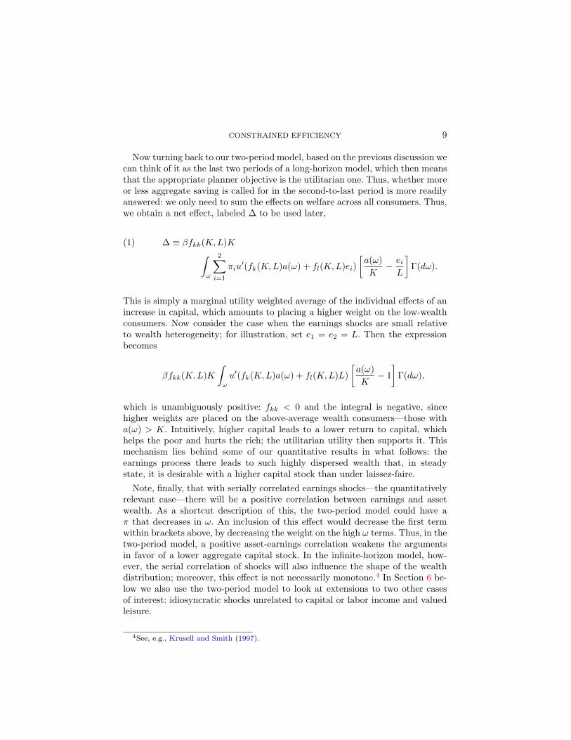
which is unambiguously positive: fkk < 0 and the integral is negative, sincehigher weights are placed on the above-average wealth consumers—those witha(ω) > K. Intuitively, higher capital leads to a lower return to capital, whichhelps the poor and hurts the rich; the utilitarian utility then supports it. Thismechanism lies behind some of our quantitative results in what follows: theearnings process there leads to such highly dispersed wealth that, in steadystate, it is desirable with a higher capital stock than under laissez-faire.
Note, finally, that with serially correlated earnings shocks—the quantitativelyrelevant case—there will be a positive correlation between earnings and assetwealth. As a shortcut description of this, the two-period model could have aπ that decreases in ω. An inclusion of this effect would decrease the first termwithin brackets above, by decreasing the weight on the high ω terms. Thus, in thetwo-period model, a positive asset-earnings correlation weakens the argumentsin favor of a lower aggregate capital stock. In the infinite-horizon model, how-ever, the serial correlation of shocks will also influence the shape of the wealthdistribution; moreover, this effect is not necessarily monotone.4 In Section 6 be-low we also use the two-period model to look at extensions to two other casesof interest: idiosyncratic shocks unrelated to capital or labor income and valuedleisure.
4See, e.g., Krusell and Smith (1997).

10 DAVILA ET AL.
2.3. The constrained optimum and implementation
On the basis of the above discussion, we define the constrained optimum bythe solution to
maxa(ω)
∫ω
[u(ω − a(ω)) + β
2∑i=1
πiu(fk(K,L)a(ω) + fl(K,L)ei)
]Γ(dω),
where K =∫ωa(ω)Γ(dω) and L = πe1 + (1 − π)e2. Here, thus, the planner
chooses a function a(ω), i.e., saving for all consumers, in order to maximize autilitarian objective. Again, the utilitarian objective may seem unmotivated inthe two-period model, but the idea, elaborated on above, is that this two-periodmodel represents the last two periods of a longer-horizon problem of which attime zero all consumers were equal.5
Given our INADA conditions on utility, we obtain interior solutions and atypical first-order condition then reads
u′(c(ω)) = β (πu′(c1(ω)) + (1− π)u′(c2(ω))) fk(K,L) + ∆,
where c(ω) ≡ ω − a(ω) and ci(ω) ≡ fk(K,L)a(ω) + fl(K,L)ei, i = 1, 2, and ∆equals the expression in (1). Notice here that ∆ does not depend on ω: the addedbenefit (if ∆ > 0), or cost (if ∆ < 0), of saving is the same for all consumers.The constrained optimum can be interpreted as attained through a direct
mandate for each consumer, issued by the planner, how to save. It can also beobtained through explicit tax incentives. The key feature of the tax system is toallow the first-order condition above to be satisfied for all consumers. This willbe accomplished by a tax wedge on the saving decision, which we can define asproportional capital income, accompanied by a lump-sum transfer so that thenet transfer to the agent is zero. The tax wedge will need to depend on individualhistories, here represented by individual beginning of period wealth: τ(ω) willappear in the Euler equation as
u′(c(ω)) ≡ β (πu′(c1(ω)) + (1− π)u′(c2(ω))) fk(K,L)(1− τ(ω)),
so that, now again rewriting using χ(ω) to denote the ratio of marginal utilitiesacross states 1 and 2 (a number greater than 1), we obtain by also imposing theconstrained-optimal first-order condition that
(2) τ(ω) = −fkk(K,L)K
fk(K,L)∫ω
u′(c2(ω))
u′(c2(ω))
π(χ(ω)− 1)(
a(ω)K − e1
L
)+ a(ω)
K − 1
π(χ(ω)− 1) + 1Γ(dω).
5Formally, one could specify an ex ante stage where all consumers would be identical and alottery mechanism that would deliver the ω distribution as an outcome. Such a model wouldformally justify the above objective but not add anything of essence.

CONSTRAINED EFFICIENCY 11
The lump-sum transfer must equal τ(ω)a(ω)fk(K,L).6
It is instructive to revisit our special cases here. First, if there is no wealthheterogeneity, we obtain
τ = −fkk(K,L)K
fk(K,L)
π(χ− 1)(1− e1
L
)π(χ− 1) + 1
> 0,
and, second, if there is wealth heterogeneity but there are no income shocks,
τ(ω) = −fkk(K,L)K
fk(K,L)
∫ω
u′(c2(ω))
u′(c2(ω))
(a(ω)
K− 1
)Γ(dω) < 0.
Thus, the optimum in the first case is attained with a proportional tax on capitalincome. In the second case, the optimum demands a subsidy, which moreoveris higher for consumers with high initial wealth. Richer consumers necessitate ahigher subsidy (and lump-sum tax) because the societal payoff ∆ from increasingsaving beyond what would be in the self-interest of the consumer, as notedabove, does not depend on this consumer’s wealth, and thus it is larger for richerconsumers, since their private marginal utility is lower. The second exampleillustrates that, in general, “simple” uniform (across types) policies do not sufficefor achieving the constrained optimum.
3. THE INFINITE-HORIZON ECONOMY
We now study the infinite-horizon version of the above model. As above, welook at a continuum of agents subject to idiosyncratic shocks ei ∈ E, whereE ≡ e1, · · · , ei, · · · , eI, that are i.i.d. across agents and that follow a Markovprocess with transition matrix πi,j . Agents have standard preferences: an ex-pected discounted sum of a strictly increasing and strictly concave utility func-tion, i.e., IE0
∑t βt u(ct). Agents do not have access to state-contingent
contracts but can only accumulate assets in the form of real capital; we denoteit a. There is a lower bound on asset holding: a.7 As in the previous section,these assets are rented by competitive firms each period and used for produc-tion purposes according to a CRS neoclassical production function f that usescapital and efficient units of labor. Capital accumulation is assumed to follow ageometric structure: a fraction δ of the capital stock depreciates from one periodto the next.8
The nature of the budget constraint that agents face is thus c + a′ = a(1 +r) + ew, where we use primes to denote the next period’s values. Individual
6Of course, the timing of the transfer is immaterial when there are no borrowing constraints;only the present value matters.
7This lower bound may arise from the existence of a solvency constraint that requires thatagents are always able to pay back their debt or from an explicit borrowing constraint.
8Note that the assumptions in the previous section can be thought of as assuming 100%depreciation, or that alternatively f was defined to include undepreciated capital.

12 DAVILA ET AL.
agents are indexed by the pair e, a that describes their labor endowment andwealth, respectively. The state of the economy can be summarized by probabilitymeasure x over the Borel sets of compact set S = E×A. In this context, aggregateamounts of factors of production and their rental prices are K =
∫Sadx, L =∫
Sedx, r = fK(K,L) − δ, and w = fL(K,L), respectively. We use the notation
r(x) and w(x), though on occasion we use r(K) and w(K), since L is constantdue to the law of large numbers.In this economy the aggregate state variable is the distribution of agents over
labor earnings and wealth, x, which agents have to know in order to computeprices.9 We write x′ = H(x) to describe the law of motion of the distribution.Then, the agent’s problem is
v(x, e, a) = maxc≥0
a′∈A
u (c) + β∑e′
πe,e′ v(x′, e′, a′) s.t.(3)
c+ a′ = a [1 + r (x)] + e w (x) and x′ = H(x),(4)with solution a′ = h(x, e, a). An important feature of this problem is the require-ment that the agent’s assets lie in compact set A.We now turn to the construction of an aggregate law of motion of the econ-
omy. Using decision rule h and transition matrix π, we construct an individualtransition process. Let B ∈ S be a Borel set. Define Q by
(5) Q(x, e, a,B;h) =∑
e′∈Be
πee′ χh(x,e,a)∈Ba,
where χ is the indicator function. It is easy to see that Q is indeed a transitionfunction. We now define the updating operator T (x,Q) that yields tomorrow’sdistribution given today’s:
(6) x′(B) = T (x,Q)(B) =
∫S
Q(x, e, a,B;h) dx.
An equilibrium requires that agents’ expectations are correct. Formally,
Definition 3. A recursive competitive equilibrium is a pair of functions h andH such that h solves problem (3) given H and that H(x) = T (x,Q(.;h)).
A steady state for this economy is a distribution x such that x = T (x, Q).Steady states have the property that the interest rate is lower than the rate oftime preference, or that the aggregate capital stock is higher than that of aneconomy with perfect markets or no shocks (for a discussion and a proof of thisresult, see Huggett (1997)). The interpretation of this result is one of precau-tionary saving : savings play dual roles here, by allowing not just intertemporalsmoothing but also some (limited) amount of smoothing across states.
9While prices today can be known just from today’s aggregate capital, future prices cannotbe known from today’s aggregate capital because decision rules are not linear. Hence, thedistribution is the appropriate state variable. See Krusell and Smith (1997), Krusell and Smith(1998), or Rıos-Rull (1998) for more elaborate discussions.

CONSTRAINED EFFICIENCY 13
3.1. Characterization: first-order conditions and steady-state capital
The consumer’s first-order condition for savings is the recursive functionalequation
u′ (x, e, a, h(x, e, a)) ≥ β[1 + r(H(x))]∑e′
πe,e′u′ (H(x), e′, h(x, e, a), h[H(x), e′, h(x, e, a)]) ,
with equality if a′ > a, which can be rewritten compactly as u′(c) ≥ β[1 +r(H(x))]
∑e′ πe,e′u
′(c).
Steady states can be readily found as a fixed point of an aggregate steady-state capital demand function, which depends on the interest rate which in turnis given by the marginal productivity of capital (see below). Let hm(e, a; r) bethe decision rule implied by a constant interest rate r (and associated wage w).It solves
(7) u′ [a(1 + r) + ew − hm(e, a; r)] ≥
β∑e′
πe,e′u′ [hm(e, a; r) (1 + r) + ew − hm[e′, hm(e, a; r); r]] ,
with equality if hm > a.
Let the stationary aggregate capital implied by hm(., .; r) be K(r), a contin-uous function of r (Rıos-Rull (1998)). A steady state is therefore characterizedby a K and a rate of return r such that given r, aggregate capital is K, i.e.,K = K(r), and r is the marginal productivity of capital implied by K, i.e.,r = fk(K, L).10
4. CONSTRAINED-OPTIMAL ALLOCATIONS IN THE INFINITE-HORIZON
ECONOMY
Our quantitative focus will be on the characterization of constrained-optimalsteady states (Section 4.3 below), i.e., long-run outcomes of a well-defined infinite-horizon planning problem. The initial condition in this planning problem is oneof complete equality across consumers—the first period of our two-period modelabove. This initial condition implies that the objective function of the plan-ner here is “utilitarian,” i.e., weighs all consumers’ utils equally. One could, ofcourse, consider arbitrary weighting schemes; our choice of equal weights is mo-tivated by our focus on insurance, as opposed to redistribution. Also as before,the planner is constrained to only consider allocations with zero net transfersacross consumers.
10In a steady state, where the discount rate exceeds the interest rate, there is an upperbound to the assets that agents hold (see Huggett (1997)).
14 DAVILA ET AL.
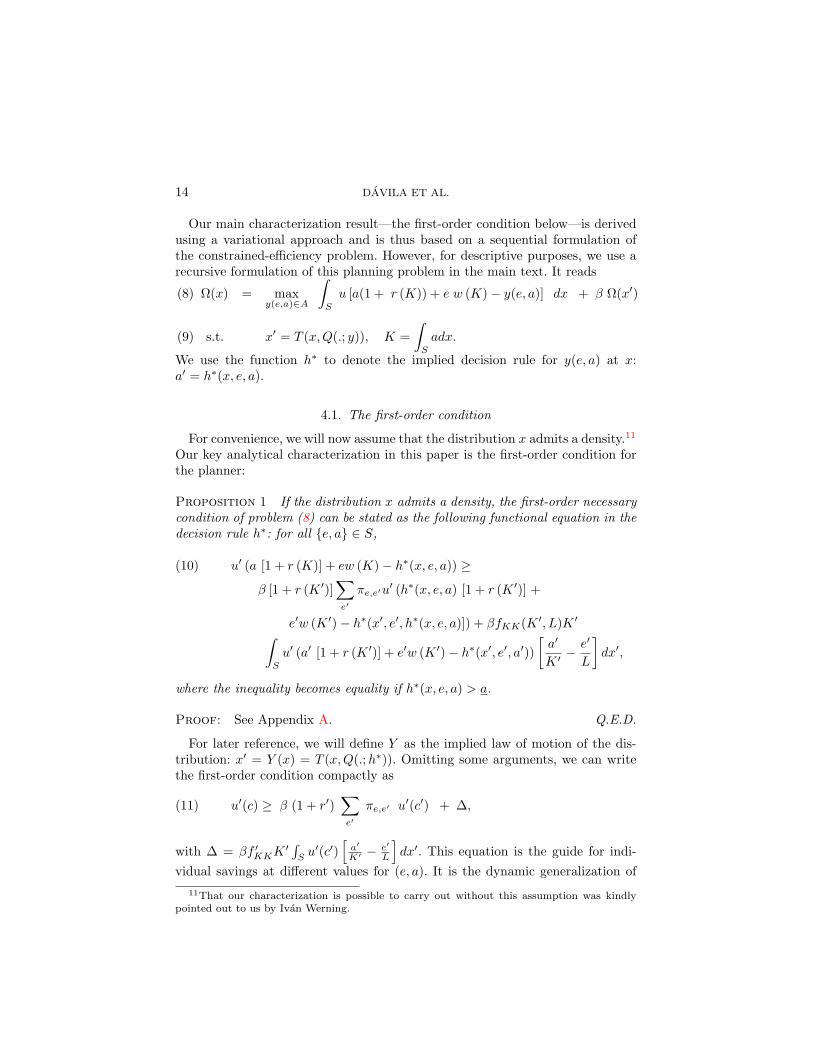
Our main characterization result—the first-order condition below—is derivedusing a variational approach and is thus based on a sequential formulation ofthe constrained-efficiency problem. However, for descriptive purposes, we use arecursive formulation of this planning problem in the main text. It reads
Ω(x) = maxy(e,a)∈A
∫S
u [a(1 + r (K)) + e w (K)− y(e, a)] dx + β Ω(x′)(8)
s.t. x′ = T (x,Q(.; y)), K =
∫S
adx.(9)
We use the function h∗ to denote the implied decision rule for y(e, a) at x:a′ = h∗(x, e, a).
4.1. The first-order condition
For convenience, we will now assume that the distribution x admits a density.11
Our key analytical characterization in this paper is the first-order condition forthe planner:
Proposition 1 If the distribution x admits a density, the first-order necessarycondition of problem (8) can be stated as the following functional equation in thedecision rule h∗: for all e, a ∈ S,
(10) u′ (a [1 + r (K)] + ew (K)− h∗(x, e, a)) ≥
β [1 + r (K ′)]∑e′
πe,e′u′ (h∗(x, e, a) [1 + r (K ′)] +
e′w (K ′)− h∗(x′, e′, h∗(x, e, a)]) + βfKK(K ′, L)K ′∫S
u′ (a′ [1 + r (K ′)] + e′w (K ′)− h∗(x′, e′, a′))
[a′
K ′ −e′
L
]dx′,
where the inequality becomes equality if h∗(x, e, a) > a.
Proof: See Appendix A. Q.E.D.
For later reference, we will define Y as the implied law of motion of the dis-tribution: x′ = Y (x) = T (x,Q(.;h∗)). Omitting some arguments, we can writethe first-order condition compactly as
(11) u′(c) ≥ β (1 + r′)∑e′
πe,e′ u′(c′) + ∆,
with ∆ = βf ′KKK ′ ∫
Su′(c′)
[a′
K′ − e′
L
]dx′. This equation is the guide for indi-
vidual savings at different values for (e, a). It is the dynamic generalization of
11That our characterization is possible to carry out without this assumption was kindlypointed out to us by Ivan Werning.

CONSTRAINED EFFICIENCY 15
the formula from our two-period model: equation (1) in particular displays thetwo-period version of the extra term, ∆, in the Euler equation. The ∆ in thetwo-period case and the one here are only different in the following two ways:(i) the probability weighting here (implicit in the dx′ expression) involves morevalues (if earnings risk is serially correlated), since the probabilities of differentoutcomes next period depend on the earnings states last period; and (ii) thejoint distribution over assets and earnings, over which the integral is defined, isdetermined more nontrivially: it depends on the entire history of shocks.Clearly, the sign of the extra term, and its magnitude, depend on the distri-
bution of agents across assets and earnings, in addition to primitives such as thecurvature of the utility function. To evaluate these, we focus on a steady-stateversion of this equation and thereafter use a calibrated version of it in orderto compare how different the long-run outcomes are between the laissez-faireallocation and the constrained optimum.
4.2. Implementation of the constrained optimum
The constrained planning allocation can be implemented with tax-transferschemes. In the two-period model, sufficient instruments involve savings wedges,along with lump-sum transfers, that depend on initial wealth, as shown in equa-tion (2). In models with more periods, the same kind of instrument can be used,the only difference being that the savings wedges (and the lump-sum transfers)now need to be history dependent.To this aim, consider the first-order condition for the constrained optimum,
i.e., condition (10). Using et to denote the complete history of productivity re-alizations for an agent, we can define the tax wedge τ(et), a tax on the grossreturn from saving decided on in period t. Using the consumer’s Euler equationfor this decision then reads
(12) u′ (c∗(x, e, a)) = β [1 + r (K ′)][1− τ(et)
]∑e′
πe,e′u′ (c∗(x′, e′, h∗(x, e, a))) ,
where we have used c∗ to denote the consumption function associated with thesavings function h∗.12 This equation awkwardly mixes recursive and sequentialnotation, but it does so for a reason. Using (10), this equation can be used tosolve out directly for taxes, state by state and period by period, as a function ofoptimal consumption-savings plans, as determined by the constrained planningproblem (where (10) is a key condition). Thus, (12) shows that the optimal taxwedge will inherit a recursive structure. In particular, one can use this equationto see that the tax rate will depend on (x, e, a): this quantity summarizes allthe necessary information in et.13 In the quantitative section below, looking at
12For cases where (10) holds with inequality there is, of course, a range of tax rates thatcould be used.
13Of course, using this dependence explicitly in the formulation of the consumer’s problemwould not be possible without somehow making clear that these tax rates are given, and notpossible to influence by the saving choice.

16 DAVILA ET AL.
steady states, we will illustrate numerically how the tax wedges computed bythe above formula depend on e and a.
4.3. The constrained-efficient steady state
A steady state for the planner is a decision rule h∗ and an associated distribu-tion x∗ such that x∗ = Y (x∗) and h∗(e, a) = h∗(x∗, e, a). With K∗ ≡
∫S
a dx∗,a steady state satisfies
(13) u′ (a [1 + r(K∗)]+ ew
(K∗)− h∗ (e, a)
)≥ β[1 + r(K∗)]∑
e′
πe,e′u′ (h∗(e, a)
[1 + r
(K∗)]+ e′w
(K∗)− h∗(e′, h∗(e, a))
)+∆,
where
∆ = Kfkk
∫S
u′ (a′ [1 + r(K∗)]+ e′w (K∗)− h∗(e′, a′)
) [ a′
K∗ − e′
L
]dx∗.
This is a functional equation that can be solved using standard numerical meth-ods. Note in this context that if ∆ is positive, there is no guarantee that thereexists an upper bound to individual asset holdings. However, an upper boundcan be imposed, and in the numerical simulations one would then verify whetheror not it is violated.The object of study in our steady-state analysis is a “modified Golden Rule,”
i.e., a long-run outcome that is optimal from the perspective of taking discountinginto account. In other words, our constrained-optimal steady state is not derivedsimply from maximizing steady-state utility without regard to initial conditionsand the costs or benefits of reaching that steady state. Instead, it answers thequestion: if the allocation that is ex ante constrained optimal has the propertythat there is convergence to a steady state, what are the properties of the impliedsteady-state distribution? Next, we answer this question quantitatively, and wealso show what kind of tax system would implement the allocation.
5. QUANTITATIVE ANALYSIS BASED ON CALIBRATIONS TO U.S. DATA
In an economy calibrated to actual data, is capital accumulation too high or toolow from a constrained-efficiency perspective? In this section we show that theanswer is sensitive to the calibration entertained, and we explain the intuitivereasons for these differences. We consider three calibrations, all of which are“standard” calibrations in the literature, emphasizing different kinds of wage-income risk. The first one is an economy where labor income is a two-stateprocess, interpretable as employment/unemployment. This economy turns outto have the property of the simplest of the two-period models in Section 2: it hastoo much capital. The second economy emphasizes asymmetric wage risk of thesort that generates a realistic (i.e., very high) wealth dispersion. In this economy,

CONSTRAINED EFFICIENCY 17
capital accumulation is much too low. In the third economy—an economy withindividual wage risk calibrated to be symmetric, as in Aiyagari (1994), thusgenerating much less wealth dispersion—capital accumulation is also too low.However, this economy has a new feature: the constrained-efficient steady stateis only asymptotic, i.e., there is ever-increasing wealth dispersion. Thus, standardcalibrations can give rise to a constrained-efficient policy that implies (i) thatcapital accumulation should be counteracted or promoted and (ii) that wealthinequality should be contained or made to grow without bound.
We display our results in Sections 5.1–5.3. We then explain and compare theseoutcomes in Section 5.4 in terms of the properties of ∆, the key ingredient inthe constrained planner’s first-order condition and other features of the differenteconomies.
5.1. The market economy has too much capital: the unemployment economy
In this economy, preferences are of the constant relative risk aversion (CRRA)
form,∑
t βt c1−σ
t −1
1−σ , with the period set to be one year. Production occurs
through a standard neoclassical production function F (Kt, Lt) = Kθt L1−θ
t . Cal-ibration of the above parameters and the rate of capital depreciation is ratherstandard: the steady state of the laissez-faire economy is targeted to a real in-terest rate of 4%, a capital-output ratio of slightly below 3, and a labor share of0.64, which is accomplished assuming that β = 0.887, δ = 0.08, and θ = 0.36,and the intertemporal elasticity of substitution is set to 0.5.
In the unemployment economy, the idiosyncratic shock captures unemploy-ment risk rather than wage risk: it can take only two values, with a very low valueof unemployment, as in Krusell and Smith (1998) or Castaneda, Dıaz-Gimenez,and Rıos-Rull (1998). This calibration interprets all the earnings volatility anddispersion as coming from shocks. We set the unemployment rate to 5% and theaverage duration of unemployment to as high as 2.6 years, thus targeting “long-term unemployment,” which exhibits long duration and is also viewed as highlycyclical. By construction, our calibration thus makes unemployment a relativelysevere shock, indeed more severe in terms of income losses than what it appearsto be for the average unemployed. The parameters involved are e = [0.01 1.00]for the labor endowment (unemployed, employed) and Π1,· = [0.62 0.38] andΠ2,· = [0.02 0.98] for the transition matrix. Table I displays the results.
As can be seen in Table I, the constrained optimum requires a lower long-run level of capital than what is generated in the laissez-faire economy. Thus,the prescription here is to move toward the first-best level of capital. Note alsothat the implied effect of constrained-optimal policy on inequality is minor. Thissupports the notion that the key determinant is the factor composition of theincome of the poor. In this model economy, the poor are unemployed and theirlabor income is essentially zero. This makes the model economy de facto capitalintensive.

18 DAVILA ET AL.
5.2. The market economy has much too little capital: high wealth dispersion
It is not immediate how to generate equilibrium wealth dispersion of a magni-tude similar to that in the data. The literature offers several possibilities; here,we follow the approach in Diaz, Pijoan-Mas, and Rıos-Rull (2003), which is asimplified version of that in Castaneda, Dıaz-Gimenez, and Rıos-Rull (2003).The general idea is (i) to include very large wage outcomes and that (ii) fromthe very high wage outcomes there is a significant risk of a large fall in the wage.The combination of these features makes the highest earners have a significantdemand for precautionary saving.14 Thus, a properly chosen three-state Markovchain allows us to generate a laissez-faire steady state with inequality measuresfor earnings and wealth quite close to those in the U.S. data. Let the three lev-els of earnings be 1.00, 5.29, 46.55; let there be no direct transitions betweenthe highest and lowest state; let the probability of staying be 0.992, 0.98, and0.917 in the low, middle, and high states, respectively, and let the transitionprobability from middle to low be 0.009. Then the stationary distribution isπ⋆ = 0.498, 0.443, 0.059. This process has an earnings Gini index of 0.60, thereis strong persistence, and there is a nontrivial risk of dropping from the higheststate to the middle state. The results for the economy calibrated in the mannerjust described are shown in Table II.
The first notable finding is that the market economy has large precautionarysavings in steady state: aggregate wealth is 2.33 times larger than in the economywithout shocks. As a result of the additional capital, output is 35.5% higher. Wealso see that the wealth Gini index of the market economy is quite large, 0.861,slightly larger than the 0.803 of the U.S. economy whereas the share of wealthheld by the richest 5% is 54.55 while in the data it is 57.80%.
Second, the constrained optimum requires an even higher level of capital inthe long run: it is as much as 8.5 times that in the deterministic economy andeven 3.65 times that in the laissez-faire allocation. These differences are verylarge. The wealth distribution in the market and the constrained-optimal allo-cations are very similar. This fact ultimately derives from the constraint on theplanner, which is precisely that no direct redistribution be made across agents:all redistributions occur through price changes.
To summarize, the constrained-efficient steady state of the model economy hasmuch more capital than does the laissez-faire steady state (which itself has muchmore capital than does the first-best steady state, due to precautionary savings).At the same time, the distribution of wealth as measured by the shares owned bythe various groups is very similar. Thus, the laissez-faire precautionary savingseconomy is associated withmuch too little capital: the pecuniary externality fromsavings in this economy is not only positive but also large.
14Wealth heterogeneity can also, for example, result from discount factor heterogeneity,as modeled in Krusell and Smith (1998). Such an assumption embodies the idea that “thewealth-poor are poor because they chose to become poor”; in the present calibration, thepoorest consumers have simply been unlucky with their earnings realizations.

CONSTRAINED EFFICIENCY 19
For this economy, we also illustrate the tax implementation discussed in Sec-tion 4.2. Figure 1 plots different subsidy wedges (net-of-tax returns), all positivehere since there is capital underaccumulation, for different individuals. Luckierconsumers, as measured either by wealth or by current labor productivity, ob-tain larger wedges, and the wedges are over 14 percentage points for the luckiestconsumers. The pre-subsidy real interest rate, which is indicated by the dottedline in Figure 1, is negative here—a little below -2%—and some of the least luckyconsumers apparently indeed do not obtain much more even after the subsidy.
5.3. Ever-increasing wealth dispersion: the original Aiyagari (1994) calibration
Using an AR(1) process in the logarithm of labor income with normally dis-tributed (symmetric) shocks, Aiyagari (1994) selects the persistence and volatil-ity parameters based on Kydland (1984), who uses the Panel Study of IncomeDynamics (PSID), and on Abowd and Card (1987) and Abowd and Card (1989),who use both PSID and National Longitudinal Surveys (NLS) data. Aiyagarithen approximates this process using a seven-state Markov chain following theprocedures described in Tauchen (1986). We follow the same procedure, althoughwe reduce the Markov chain to three states. We take our benchmark to have anautocorrelation of 0.6 and a coefficient of variation of 0.2.15 We specify the otherparameters so that the economy with complete markets (the standard neoclassi-cal growth model) satisfies standard properties. The interest rate is set to 4.167%:β is 0.96. Our only departure from Aiyagari (1994) is to set the intertemporalelasticity of substitution, 1
σ , to be equal to 0.5.16 The capital share is equal to0.36 and the capital-output ratio is set to slightly under 3.17
The asymptotic steady state of the market outcome in the Aiyagari economyhas 2.03% more assets and 0.70% more assets than its full insurance counterpart,with an interest rate of 4.011% instead of 4.167%. The implied coefficient ofvariation of wealth is 0.718 and its Gini index of wealth is 0.388, far below thedispersion observed in the data.The interesting feature of this economy, however, is that the constrained-
efficient allocation has ever-increasing wealth inequality. For this economy, first,it is possible to verify numerically that no exact steady state exists.18 Second,
15The specific parameters for the three-state process are given by e ∈ e1, e2, e3 =0.78, 1.00, 1.27, πe′|e1 = 0.66, 0.27, 0.07, πe′|e1 = 0.28, 0.44, 0.28, and πe′|e1 =0.07, 0.27, 0.66. The resulting stationary distribution is π⋆ = 0.337, 0.326, 0.337.
16Aiyagari (1994) considers the values 1, 0.33, and 0.2. Though we do not report theseresults, we have found that our Aiyagari economy does not change its qualitative features ifone changed the intertemporal elasticity of substitution to 1 or 3.
17It is set to 2.959 so that the depreciation rate of capital, δ, equals 0.08.18As for the previous economies, a steady state is computed by (i) guessing on a value
for aggregate capital and on a value for ∆, (ii) solving the constrained-efficient first-ordercondition, (iii) simulating an individual’s history long enough that the distribution acrossassets and earnings is obtained, and (iv) computing the implied aggregate capital stock and ∆.To verify that a steady state does not exist, one can search exhaustively for values of capitaland ∆.

20 DAVILA ET AL.
to solve for a constrained-efficient outcome, i.e., for the transition toward anasymptotic steady state from some given initial distribution of assets and earn-ings, we use techniques similar to those developed in Krusell and Smith (1997)and Krusell and Smith (1998); for details, see the Appendix B. For simplicity, weconsider as the initial condition the steady-state income-wealth distribution ofthe market allocation. We see from Figure 2, which describes how different mo-ments of the distribution of capital evolve, that the constrained-efficient outcomefeatures increasing wealth concentration over time, with otherwise well-behavedaggregates.19
5.4. Comparisons
The previous sections illustrate that it is nontrivial to predict the nature ofthe inefficiency in this class of models. The key object is the nature of ∆: theaverage of a/K − e/L in the population, weighted by marginal utilities. Themarginal utilities are declining in consumption, thus giving higher weight to theconsumption unlucky. The effect ∆ is fundamentally endogenous, and it turnsout that it is negative for the unemployment economy but positive for the twoother economies. Hence, given that a higher ∆ in the constrained-efficient Eulerequation means a stronger incentive to save, the unemployment economy hastoo much and the other economies too little capital. Why is ∆ smaller in theunemployment economy? The determinants of ∆ were discussed in Section 2;the sign of a/K− e/L for the agents with the lowest consumption is particularlyimportant, since those agents receive the highest weight. In the unemploymenteconomy, the wealth distribution is rather tight and the poorest agents are wagepoor more than wealth poor—a/K − e/L is positive for them, and ∆ < 0.
In the economy with a realistic wealth distribution, a/K − e/L is negative forthe consumption poorest, since this economy has a very skewed wealth distribu-tion (the wage dispersion is high but is less skewed). Moreover, due to the highlyunequal wealth distribution, ∆ is quantitatively large, leading to a large discrep-ancy between the constrained optimum and the laissez-faire outcome. As we sawin Table II, capital is in fact so high in the constrained optimum that the realinterest rate is negative. In contrast, the Aiyagari (1994) economy, which alsohas ∆ > 0, has only a modest discrepancy between the savings in the constrainedoptimum and the laissez-faire; in particular, the constrained-efficient real inter-est rate here is positive. Now compare these two economies from the perspectiveof the “lucky” high-asset consumers; how can they be induced to save more, soas to raise aggregate saving beyond the laissez-faire level? In an economy witha negative real interest rate, assets must not be kept too high, since then thereis a net loss to the agent in the period budget constraint. In fact, assets mustclearly be bounded in our calibrated economy with large wealth inequality—theycannot exceed −w/r times the highest individual productivity level, which is fi-
19Appendix B illustrates transition paths for an economy with a steady state.

CONSTRAINED EFFICIENCY 21
nite. Thus, the long-run wealth distribution will necessarily keep a finite support.When the interest rate is positive, however, one can see how the support mayneed to be infinite, and wealth dispersion may need to expand indefinitely. TheEuler equation of the consumer has an additional term on the right-hand side,a term that induces more asset accumulation. That term will be more and moreimportant relative to consumption the higher is consumption, and hence an ele-ment of “increasing returns to asset accumulation” has been introduced on thelevel of the individual. It follows that marginal propensities to save can becomeincreasing in wealth. Whether this effect is strong or not depends on ∆ and on theinterest rate. A higher interest rate will make at+1 − at = wet − ct + rat greater;it will also be increasing in asset holdings, unless the marginal propensity to con-sume out of asset holdings is above the interest rate, an undesirable feature fromthe perspective of consumption insurance. Thus, ever-increasing wealth for theluckiest is an outcome that is consistent with achieving constrained efficiency.The economy that delivers a more realistic wealth distribution—with high
dispersion—features saving rates that are, relative to the other economies stud-ied, higher for the rich and lower for the poor. Overall, however, in steadystate saving remains too low. This raises two questions. One is how the higher,constrained-optimum level of capital is raised—by making all the consumers savemore or by differentiated saving responses among the rich and the poor? Inter-estingly, the answer is that the constrained optimum dictates that the rich aremade to save even more but that the poor are made to lower their saving. Thisresult is apparent from comparing the steady-state decision rules in laissez-faireto those in the constrained optimum and can be understood from looking atthe Euler equations of the poor and the rich. Here, the added marginal utilitybenefit from saving, ∆, has a larger effect on the rich, as the other terms of theirEuler equation are small, i.e., their marginal utilities are low. Wealth dispersion,however, barely changes because even though the rich save more, the returns tobeing lucky fall considerably with the higher capital stock. The second questionthat arises as a result is whether the underlying reason for the dispersion insaving rates among the rich and the poor matters for our undersaving result. Itmay indeed matter, and we discuss this issue briefly in the concluding section ofthe paper.
6. EXTENSIONS
In this section, we very briefly look at two extensions of relevance. The first ofthese is one with valued leisure, a setting commonly used in the recent literature;the second looks at other kinds of shocks. The two-period model is used forillustration, and we abstract from initial wealth heterogeneity.Suppose consumers have period utility u(c, 1− l), where l is labor supplied to
the market. For simplicity, let labor supply be a choice variable only in the secondperiod; in the first period, it is fixed at some exogenous value l. This economy thusincorporates another “insurance channel” through the hours choice: in response

22 DAVILA ET AL.
to the income shock, the consumer can choose to work more.20 An equilibriumhere is defined as follows:
Definition 4. A competitive equilibrium is a vector (K, r,w, L1, L2) such that(i) (K,L1, L2) solves
maxa,l1,l2
u(ω−a, 1− l)+β (πu(ra+ we1l1, 1− l1) + (1− π)u(ra+ we2l2, 1− l2))
and (ii) r = fk(K,L) and w = fl(K,L), with L = πe1L1 + (1− π)e2L2.
Similarly, along the above lines, we can derive the first-order condition for theconstrained optimum. For capital, we obtain
(14) u′(c∗, 1− l) = β (πu′(c∗1, 1− l∗1) + (1− π)u′(c∗2, 1− l∗2)) + ∆k,
where
∆k = βu′(c∗2, 1− l∗2)π(χ− 1)
(1− e1l
∗1
L
)fkk(k
∗, l∗)k∗,
with c∗ = ω − k∗, ci = fk(k∗, l∗)k∗ + fl(k
∗, l∗)ei, i ∈ 1, 2, and χ = u′(c∗1, 1 −l∗1)/u
′(c∗2, 1− l∗2). For labor, we obtain, for i ∈ 1, 2,
(15) u1−l(c∗i , 1− l∗i ) = u′(c∗i , 1− l∗i )fl(k
∗, l∗)ei +∆l,
with
∆l = u′(c∗2, 1− l∗2)π(χ− 1)
(e1l
∗1
L− 1
)fll(k
∗, l∗)l∗.
Here, clearly, ∆k and ∆l represent deviations from the laissez-faire first-orderconditions. Somewhat more stringent conditions are needed to sign these termsthan in the case without valued leisure, but standard calibrations would imply(i) that u′(c∗1, 1 − l∗1) > u′(c∗2, 1 − l∗2) (recall that e2 > e1), so that χ > 1, and(ii) that e1l1 < e2l2. Thus, we would have, as before, that ∆k < 0, whereas∆l > 0: in the absence of wealth heterogeneity, capital is still overaccumulatedin equilibrium, and moreover consumers work too little. Additional work effortwould lower wages, which would reduce the risky part of consumers’ income. Forspecific parametric examples, with a constant elasticity of substitution betweenc and 1 − l or the case where there are no wealth effects on labor supply, it iseasy to show that these properties are met.Turning to the second and last extension, consider shocks that do not influence
either labor or capital income. First, consider a “health expenditure shock” thatappears as a negative income shock: second-period income is now ra+w−e, wheree is either high or low. In the absence of other shocks, the laissez-faire equilibrium
20For an analysis of this kind of mechanism, see, e.g., Domeij and Floden (2006), Pijoan-Mas(2006), or Heathcote, Storesletten, and Violante (2009).

CONSTRAINED EFFICIENCY 23
is now constrained efficient. A change in savings away from equilibrium wouldchange r and w as before, but ∆ = 0 would result, since the sum of capitaland labor income would not be influenced by the price changes on the margin.With more than two periods, however, health expenditure shocks would lead toa constrained-inefficient equilibrium: now savings would be too low, since healthshocks do generate capital income dispersion in periods after the second period,and the risk implied by this dispersion would be counteracted by higher aggregatesaving (through a reduction in r). Second, consider multiplicative taste shocks:period 2 utility is now u(c)e, where e is again either high or low. As for healthexpenditure shocks, the laissez-faire equilibrium would be constrained efficientin the two-period model: price changes induced by altered aggregate savingswould not influence consumers’ income on the margin. In longer-horizon models,there would be non trivial effects, since the taste shocks—which can now also beinterpreted as shocks to discounting—would induce differences in saving. Thus,changes in aggregate saving, again through prices, will have different impactson different consumers and will be a valuable instrument for the planner. Itwould be interesting to study this case, as well as the interaction of shocks, in along-horizon model in much more detail.
7. CONCLUSION
In this paper, we have argued that the laissez-faire competitive equilibriumof the one-sector neoclassical growth model with uninsurable idiosyncratic wageshocks, which plays a prominent role in the recent macroeconomic literature, mayoffer significant scope for welfare improvements. Obviously, welfare improvementscould be achieved by simply adding insurance markets—or, equivalently, by usingtax-transfer schemes that effectively distribute from the lucky to the unlucky—but what we argue here is that improvements can be made without alteringthe market structure, and without forcing any transfers between consumers.That is, we argue that the equilibrium is constrained inefficient, in the sense ofDiamond (1967): if consumers merely departed somewhat from their individualoptimization, equilibrium prices would be altered and everybody’s welfare wouldrise. The reason is that this model has a “pecuniary externality”: with incompletemarkets, the price mechanism does not fully work. In particular, the uninsurablerisk agents face can be made more or less hurtful by altering prices.In the standard setting we look at, the risk appears through prices. The direct
risk in the model is wage risk, but the insurability of this risk also induces wealthdifferences, and the propagation of this wealth inequality critically depends onthe interest rate. Therefore, whether it is beneficial to raise wages or interestrates depends on the details of the model calibration. We derive the constrainedplanner’s first-order condition, and it reveals whether savings should be increasedor decreased relative to laissez-faire. The key here is whether the consumption-poor consumers—who define the “unlucky” in this economy—have lower laborearnings or asset holdings relative to the average consumer. We illustrate with

24 DAVILA ET AL.
three standard calibrations from the literature and show that these calibrationsgive rise to very different qualitative as well as quantitative results. For the cali-bration that arguably best fits the data on inequality, the constrained optimumcalls for a rather large increase in overall savings relative to the laissez-faireoutcome.It is important to relate our study to existing tax policy analyses using similar
models. Given that our focus is on individual uninsurable risks, there is no directconnection to representative agent treatments such as the classic zero-capital taxresult in Chamley (1986). The most closely related studies are arguably Aiya-gari (1995) and Aiyagari and McGrattan (1998). Aiyagari (1995) argues for a taxon capital using a model where consumer utility also depends on endogenouslychosen government expenditures. Since an Euler equation has to hold for govern-ment expenditures, and there is no aggregate uncertainty, the government hasno precautionary savings motive, and hence it is optimal to tax savings so as tobring the economy to the first-best level of aggregate capital: the interest rate hasto equal the time discount rate. Aiyagari’s tax policy, unlike ours, also involvesnet transfers across consumers. the study of Aiyagari and McGrattan (1998) isalso different from our study in that it does not insist on zero net transfers acrossconsumers; moreover, it has government expenditures, though modeled to be aconstant percentage of output. Debt has a variety of effects; among others, itlowers the capital stock, and it requires financing, which under the lump-sumtax scheme considered by the authors hurts the poor disproportionately. Over-all, the authors find debt to have a small effect on welfare compared to actualU.S. debt policy. Other related studies include those on unemployment insur-ance (see, e.g., the recent overview in Mukoyama (2010)), progressive taxation,social security, and so on. In all these studies, the precise restrictions placed ongovernment policy are crucial and dictate what constitutes optimal policy. Ourrestriction—that no net transfers be made across consumers and only the exist-ing market structure be used—is different in that it focuses more narrowly onthe question of what “pecuniary externalitities” operate in the missing-marketseconomy. In any applied studies of the effect of tax-transfer changes, one of thechannels is the one we focus sharply and uniquely on here, though other channelswill typically be present in those studies as well.Our findings raise several questions worthy of further research. One regards
the source of idiosyncratic risks. The standard model under study here looks atwage/unemployment shocks, but consumers are subject to other risks as well.In Section 6 we briefly consider “expenditure shocks,” which do not operatethrough prices, and find constrained efficiency. Relatedly, it would be valuable togo beyond the consumption-saving choice and look at other decisions such as thelabor-leisure choice and the education choice, both of which might be associatedwith constrained inefficiency. We look at the labor-leisure choice in the context ofthe two-period model (in Section 6) and find that consumers “underwork”: takingthe effect of wages on the de facto wage risk into account, everybody’s utilitywould increase with slightly higher work effort than in a laissez-faire equilibrium.

CONSTRAINED EFFICIENCY 25
Our analysis here just scratches the surface of an interesting problem; a moreambitious analysis of this issue is under way by Athreya, Tam, and Young.Another interesting possibility is that idiosyncratic, uninsurable income may leadto constrained inefficiency even in the absence of capital accumulation. A veryrecent paper, Farinha Luz and Werquin (2011), shows that the Huggett model(Huggett (1993), which does not have capital accumulation) can be constrainedinefficient too: utility can go up for all agents if a stricter borrowing constraintis “self-imposed.”
An equally important issue concerns the calibration. Our calibration wherewealth dispersion is as large as in the data follows Castaneda, Dıaz-Gimenez,and Rıos-Rull (2003), which relies on risks of large (but infrequent) hikes anddrops in earnings. There are alternative ways of explaining the wide dispersionin wealth that we observe in most economies, and it would be interesting toconsider constrained efficiency in such settings as well. One involves preferenceheterogeneity, where wealth inequality derives chiefly from persistent shocks topatience. A complementary assumption is that poor agents receive larger trans-fers, such as those implied by unemployment insurance or food stamp programs,leading them to save less.21 A model might give results that are quite differentfrom those we obtain here, since they suggest that wealth inequality is not alla result of incomplete risk sharing. In other words, the planner would be morewilling to let those who choose to become poor (rich) stay poor (rich).
Similarly, other forms of heterogeneity in preferences (such as risk aversion)or in individuals’ abilities or opportunities (e.g., possibly making it harder forsome to participate in asset markets than it is for others) would also be valuableto examine from the perspective of constrained efficiency. The hope is that ulti-mately, microeconomic studies allow us to better distinguish which elements ofindividual heterogeneity are key and which are not.
Finally, it is interesting to examine constrained efficiency in contexts wherethere are explicit reasons for market incompleteness, such as private informa-tion. This feature has several applications already, two of which are particularlynoteworthy. One is the work of Golosov and Tsyvinski (2007), which finds, aswe do, that there can be over- or underaccumulation of capital relative to theconstrained-efficient outcome depending on the details of the calibration (in theircase, the nature of the unobservable skill process). In contrast, in the contextof the Diamond-Dybvig model of banking, Farhi, Golosov, and Tsyvinski (2009)find interest rates in the “shadow market”—where depositors can trade amongthem without being observed by banks—to always be too high (this model, how-ever, does not have capital). Doubtlessly, many interesting applications are yetto appear in this new literature.
21These two assumptions are key in Krusell and Smith (1997) and Krusell and Smith (1998).

26 DAVILA ET AL.
REFERENCES
Abowd, J. M., and D. Card (1987): “Intertemporal Labor Supply and Long Term Employ-ment Contracts,” American Economic Review, 77, 50–68.
(1989): “On the Covariance Structure of Earnings and Hours Changes,” Econometrica,57, 411–445.
Aiyagari, S. R. (1994): “Uninsured Idiosyncratic Risk and Aggregate Saving,” QuarterlyJournal of Economics, 109, 659–684.
(1995): “Optimal Capital Income Taxation with Incomplete Markets, Borrowing Con-straints, and Constant Discounting,” Journal of Political Economy, 103, 1158–1175.
Aiyagari, S. R., and E. R. McGrattan (1998): “The optimum quantity of debt,” Journalof Monetary Economics, 42, 447–469.
Bewley, T. (1986): “Stationary Monetary Equilibrium with a Continuum of IndependentlyFluctuating Consumers,” in Contributions to Mathematical Economics in Honor of GerardDebreu, ed. by W. Hildenbrand, and A. Mas-Colell. North Holland, Amsterdam.
Carvajal, A., and H. M. Polemarchakis (2011): “Idiosyncratic Risk and Financial Policy,”Journal of Economic Theory, 146, 1569–1597.
Castaneda, A., J. Dıaz-Gimenez, and J.-V. Rıos-Rull (1998): “Exploring the Income Dis-tribution Business Cycle Dynamics,” Journal of Monetary Economics, 42, 90–130.
Castaneda, A., J. Dıaz-Gimenez, and J. V. Rıos-Rull (2003): “Accounting for the U.S.Earnings and Wealth Inequality,” Journal of Political Economy, 111, 818–857.
Chamley, C. (1986): “Optimal Taxation of Capital Income in General Equilibrium with Infi-nite Lives,” Econometrica, 54, 607–622.
Diamond, P. (1980): “Efficiency with Uncertain Supply,” The Review of Economic Studies,47, 645–651.
Diamond, P. A. (1967): “The Role of a Stock Market in a General Equilibrium Model withTechnological Uncertainty,” American Economic Review, 57, 759–776.
Diaz, A., J. Pijoan-Mas, and J.-V. Rıos-Rull (2003): “Precautionary Savings and WealthDistribution under Habit Formation Preferences,” Journal of Monetary Economics, 50,1257–1291.
Domeij, D., and M. Floden (2006): “The Labor-Supply Elasticity and Borrowing Con-straints: Why Estimates Are Biased,” Review of Economic Dynamics, 9, 242–262.
Farhi, E., M. Golosov, and A. Tsyvinski (2009): “A Theory of Liquidity and Regulationof Financial Intermediation,” Review of Economic Studies, 76, 973–992.
Farinha Luz, V., and N. Werquin (2011): “Constrained Inefficiency in a Huggett Model,”Working Paper, Yale University.
Geanakoplos, J., M. Magill, M. Quinzii, and J. Dreze (1990): “Generic Inefficiency ofStock Market Equilibrium When Markets Are Incomplete,” Journal of Mathematical Eco-nomics, 19, 113–151.
Geanakoplos, J., and H. M. Polemarchakis (1986): “Existence, Regularity, and Con-strained Suboptimality of Competitive Allocations when the Asset Market is Incomplete,” inEssays in Honor of Kenneth Arrow Vol. 3 Uncertainty, Information, and Communication,ed. by W. Heller, R. Starr, and D. Starrett, pp. 65–95. Cambridge: Cambridge UniversityPress.
Golosov, M., and A. Tsyvinski (2007): “Optimal Taxation with Endogenous InsuranceMarkets,” Quarterly Journal of Economics, 122, 487–534.
Greenwald, B. C., and J. E. Stiglitz (1986): “Externalities in Economies with ImperfectInformation and Incomplete Markets,” Quarterly Journal of Economics, 101, 229–264.
Hart, O. D. (1975): “On the Optimality of Equilibrium When the Market Structure is Incom-plete,” Journal of Economic Theory, 11, 418–443.
Heathcote, J., K. Storesletten, and G. L. Violante (2009): “Consumption and LaborSupply with Partial Insurance: An Analytical Framework,” Working Paper 15257, NationalBureau of Economic Research.
Huggett, M. (1993): “The Risk-Free Rate in Heterogeneous-Agent, Incomplete-InsuranceEconomies,” Journal of Economic Dynamics and Control, 17, 953–970.

CONSTRAINED EFFICIENCY 27
(1997): “The One-Sector Growth Model with Idiosyncratic Shocks: Steady States andDynamics,” Journal of Monetary Economics, 39, 385–403.
Imrohoroglu, A. (1989): “Cost of Business Cycles with Indivisibilities and Liquidity Con-straints,” Journal of Political Economy, 97, 1364–1383.
Krusell, P., and A. A. Smith (1997): “Income and Wealth Heterogeneity, Portfolio Choice,and Equilibrium Asset Returns,” Macroeconomic Dynamics, 1, 387–422.
(1998): “Income and Wealth Heterogeneity in the Macroeconomy,” Journal of PoliticalEconomy, 106, 867–896.
Kydland, F. E. (1984): “Labor-Force Heterogeneity and the Business Cycle,” Carnegie-Rochester Conference Series on Public Policy, 21, 173–209.
Loong, L. H., and R. Zeckhauser (1982): “Pecuniary Externalities Do Matter When Con-tingent Claims Markets Are Incomplete,” Quarterly Journal of Economics, 97, 171–179.
Mukoyama, T. (2010): “Understanding the Welfare Effects of Unemployment Insurance Policyin General Equilibrium,” Working Paper, University of Virginia.
Newbery, D. M. G., and J. E. Stiglitz (1984): “Pareto Inferior Trade,” Review of EconomicStudies, 51, 1–12.
Pijoan-Mas, J. (2006): “Precautionary Savings or Working Longer Hours?,” Review of Eco-nomic Dynamics, 9, 326–352
Rıos-Rull, J.-V. (1998): “Computation of Equilibria in Heterogeneous-Agent Models,” inComputational Methods for the Study of Dynamic Economies, ed. by R. Marimon, andA. Scott, chap. 9. New York: Oxford University Press.
Stiglitz, J. E. (1982): “The Inefficiency of the Stock Market Equilibrium,” Review of Eco-nomic Studies, 49, 241–261.
Tauchen, G. (1986): “Finite State Markov-Chain Approximations to Univariate and VectorAutoregressions,” Economics Letters, 20, 177–181.

28 DAVILA ET AL.
TABLE I
Steady states for the unemployment economy
First Best Market Outcome Constrained Optimum
Aggregate assets 2.959 3.359 3.279Output 1.000 1.047 1.038Capital-output ratio 2.959 3.209 3.160Interest rate 4.167% 3.219% 3.392%Coeff. of variation of wealth 0.0 0.203 0.200Gini index for wealth 0.0 0.108 0.105
TABLE II
Steady states for the high wealth dispersion economy
First Best Market Outcome Constrained Optimum
Aggregate assets 1.736 4.017 15.668Output 1.000 1.353 2.208Capital-output ratio 1.736 2.970 7.096Real interest rate 12.740% 4.123% -2.927%Coeff. of variation of wealth 0.0 2.562 2.501Gini index for wealth 0.0 0.861 0.864Percentage of wealth of the top 5% 0.0 54.55 51.26

CONSTRAINED EFFICIENCY 29
−4 −3 −2 −1 0 1 2 3 4 5 6−6
−4
−2
0
2
4
6
8
10
12
14
log(Asset)
inte
rest
rate
(%)
lowmiddlehigh
Figure 1.— Net-of-tax returns to savings as a function of e and a.

30 DAVILA ET AL.
020
040
060
080
010
004681012
1st m
omen
t
020
040
060
080
010
000
2000
4000
6000
8000
2nd m
omen
t
020
040
060
080
010
000123456x 1
063rd
mom
ent
time
020
040
060
080
010
000123456x 1
094th
mom
ent
time
Figure 2.— Transition from the market steady state to the constrained op-timum.
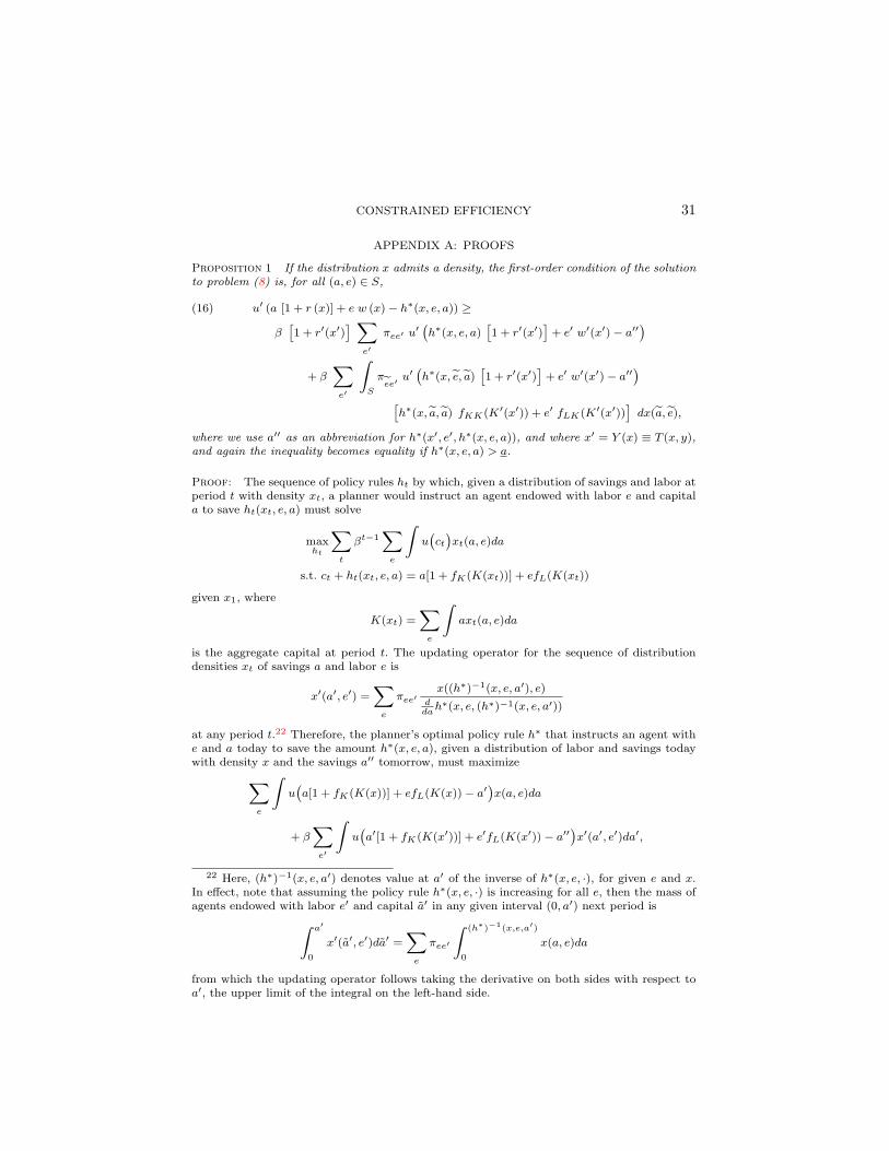
CONSTRAINED EFFICIENCY 31
APPENDIX A: PROOFS
Proposition 1 If the distribution x admits a density, the first-order condition of the solutionto problem (8) is, for all (a, e) ∈ S,
(16) u′ (a [1 + r (x)] + e w (x)− h∗(x, e, a)) ≥
β[1 + r′(x′)
] ∑e′
πee′ u′(h∗(x, e, a)
[1 + r′(x′)
]+ e′ w′(x′)− a′′
)+ β
∑e′
∫S
πee′
u′(h∗(x, e, a)
[1 + r′(x′)
]+ e′ w′(x′)− a′′
)[h∗(x, a, a) fKK(K′(x′)) + e′ fLK(K′(x′))
]dx(a, e),
where we use a′′ as an abbreviation for h∗(x′, e′, h∗(x, e, a)), and where x′ = Y (x) ≡ T (x, y),and again the inequality becomes equality if h∗(x, e, a) > a.
Proof: The sequence of policy rules ht by which, given a distribution of savings and labor atperiod t with density xt, a planner would instruct an agent endowed with labor e and capitala to save ht(xt, e, a) must solve
maxht
∑t
βt−1∑e
∫u(ct)xt(a, e)da
s.t. ct + ht(xt, e, a) = a[1 + fK(K(xt))] + efL(K(xt))
given x1, where
K(xt) =∑e
∫axt(a, e)da
is the aggregate capital at period t. The updating operator for the sequence of distributiondensities xt of savings a and labor e is
x′(a′, e′) =∑e
πee′x((h∗)−1(x, e, a′), e)
ddah∗(x, e, (h∗)−1(x, e, a′))
at any period t.22 Therefore, the planner’s optimal policy rule h∗ that instructs an agent withe and a today to save the amount h∗(x, e, a), given a distribution of labor and savings todaywith density x and the savings a′′ tomorrow, must maximize∑
e
∫u(a[1 + fK(K(x))] + efL(K(x))− a′
)x(a, e)da
+ β∑e′
∫u(a′[1 + fK(K(x′))] + e′fL(K(x′))− a′′
)x′(a′, e′)da′,
22 Here, (h∗)−1(x, e, a′) denotes value at a′ of the inverse of h∗(x, e, ·), for given e and x.In effect, note that assuming the policy rule h∗(x, e, ·) is increasing for all e, then the mass ofagents endowed with labor e′ and capital a′ in any given interval (0, a′) next period is∫ a′
0
x′(a′, e′)da′ =∑e
πee′
∫ (h∗)−1(x,e,a′)
0
x(a, e)da
from which the updating operator follows taking the derivative on both sides with respect toa′, the upper limit of the integral on the left-hand side.
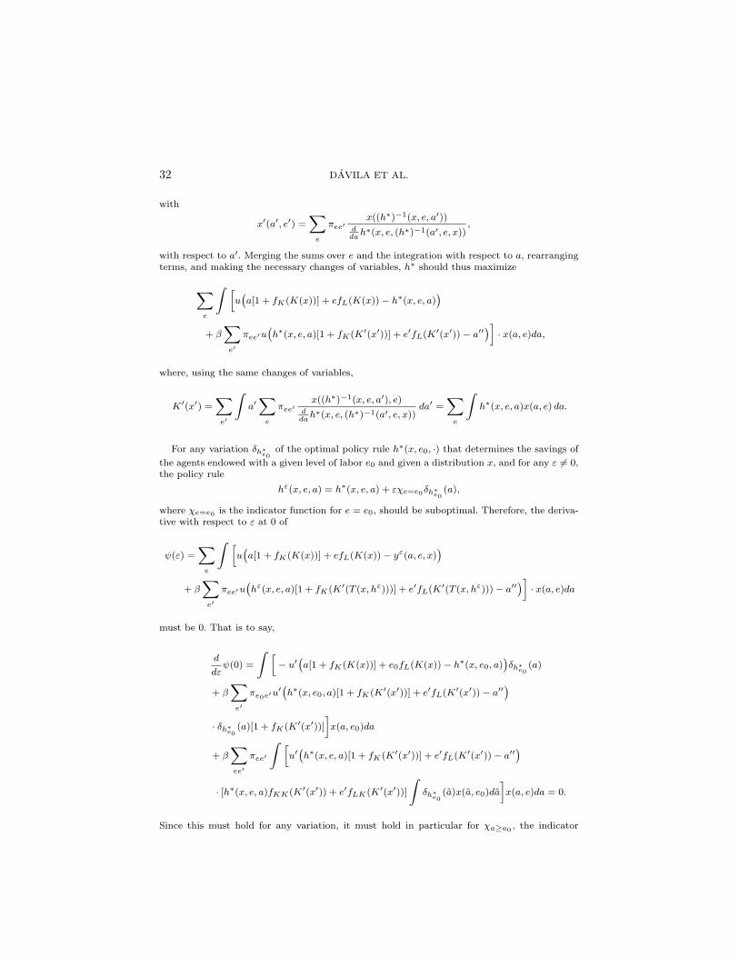
32 DAVILA ET AL.
with
x′(a′, e′) =∑e
πee′x((h∗)−1(x, e, a′))
ddah∗(x, e, (h∗)−1(a′, e, x))
,
with respect to a′. Merging the sums over e and the integration with respect to a, rearrangingterms, and making the necessary changes of variables, h∗ should thus maximize
∑e
∫ [u(a[1 + fK(K(x))] + efL(K(x))− h∗(x, e, a)
)+ β
∑e′
πee′u(h∗(x, e, a)[1 + fK(K′(x′))] + e′fL(K
′(x′))− a′′)]
· x(a, e)da,
where, using the same changes of variables,
K′(x′) =∑e′
∫a′∑e
πee′x((h∗)−1(x, e, a′), e)
ddah∗(x, e, (h∗)−1(a′, e, x))
da′ =∑e
∫h∗(x, e, a)x(a, e) da.
For any variation δh∗e0
of the optimal policy rule h∗(x, e0, ·) that determines the savings of
the agents endowed with a given level of labor e0 and given a distribution x, and for any ε = 0,the policy rule
hε(x, e, a) = h∗(x, e, a) + εχe=e0δh∗e0
(a),
where χe=e0 is the indicator function for e = e0, should be suboptimal. Therefore, the deriva-tive with respect to ε at 0 of
ψ(ε) =∑e
∫ [u(a[1 + fK(K(x))] + efL(K(x))− yε(a, e, x)
)+ β
∑e′
πee′u(hε(x, e, a)[1 + fK(K′(T (x, hε)))] + e′fL(K
′(T (x, hε)))− a′′)]
· x(a, e)da
must be 0. That is to say,
d
dεψ(0) =
∫ [− u′
(a[1 + fK(K(x))] + e0fL(K(x))− h∗(x, e0, a)
)δh∗
e0(a)
+ β∑e′
πe0e′u′(h∗(x, e0, a)[1 + fK(K′(x′))] + e′fL(K
′(x′))− a′′)
· δh∗e0
(a)[1 + fK(K′(x′))]
]x(a, e0)da
+ β∑ee′
πee′
∫ [u′(h∗(x, e, a)[1 + fK(K′(x′))] + e′fL(K
′(x′))− a′′)
· [h∗(x, e, a)fKK(K′(x′)) + e′fLK(K′(x′))]
∫δh∗
e0(a)x(a, e0)da
]x(a, e)da = 0.
Since this must hold for any variation, it must hold in particular for χa≥a0, the indicator

CONSTRAINED EFFICIENCY 33
function of a ≥ a0, for any a0. Therefore, rearranging terms and substituting χa≥a0for δh∗
e0,∫ +∞
a0
[− u′
(a[1 + fK(K(x))] + e0fL(K(x))− h∗(x, e0, a)
)+ β
∑e′
πe0e′u′(h∗(x, e0, a)[1 + fK(K′(x′))] + e′fL(K
′(x′))− a′′)
· [1 + fK(K′(x′))]
]x(a, e0)da
+ β∑ee′
πee′
∫ [u′(h∗(x, e, a)[1 + fK(K′(x′))] + e′fL(K
′(x′))− a′′)
· [h∗(x, e, a)fKK(K′(x′)) + e′fLK(K′(x′))]
∫ +∞
a0
x(a, e0)da
]x(a, e)da = 0.
The right-hand side of the last expression is therefore a constant function of a0 equal to 0. Asa consequence, its derivative with respect to a0 must be 0, i.e., for all a0 and all e0,
− u′(a0[1 + fK(K(x))] + e0fL(K(x))− h∗(x, e0, a0)
)+ β
∑e′
πe0e′u′(h∗(x, e0, a0)[1 + fK(K′(x′))] + e′fL(K
′(x′))− a′′)· [1 + fK(K′(x′))]
+ β∑ee′
πee′
∫u′(h∗(x, e, a)fK(K′(x′)) + e′fL(K
′(x′))− a′′)
· [h∗(x, e, a)fKK(K′(x′)) + e′fLK(K′(x′))]x(a, e)da = 0,
i.e., for all (a, e)
u′(a[1 + r(x)] + ew(x)− h∗(x, e, a)
)=
β[1 + r′(x′)]∑e′
πee′u′(h∗(x, e, a)[1 + r′(x′)] + e′w′(x′)− a′′
)+ β
∑ee′
πee′
∫u′(h∗(x, e, a)[1 + r′(x′)] + e′w′(x′)− a′′
)· [h∗(x, e, a)fKK(K′(x′)) + e′fLK(K′(x′))]x(a, e)da.
Q.E.D. Q.E.D.
APPENDIX B: APPROXIMATION METHODS
We now briefly describe how we solve the problem of the planner outside the steady state.Given V (m) for m ∈ IRnm and x, we can solve the following problem:
maxy(e,a)
∫u(a[1 + r(K)] + e w(K)− y(e, a)) dx+ β V (m′)(17)
subject to m′ = φ(x, y).(18)We select a set of momentsm ∈ IRnm of the distribution x; the moments are defined bymi =∫
Sai dx, and typically we simply choose the first three moments. We then approximate the
function V as a quadratic function of the logarithms of the chosen moments of the distribution,with some coefficient restrictions. A typical functional form that we have chosen is
V (m) = α0 + α1 log(m1) + α2 log(m
2) + α3 log(m3) + α4 log
2(m1).
To solve the planning problem and to obtain the coefficients α, we proceed as follows:

34 DAVILA ET AL.
1. Make an initial guess on V , labeled V 0. That is, guess an α0 ∈ IRnα .
2. Choose an initial distribution x0 and calculate its moments m0. Then generate a samplefor 10,000 individuals.
3. Construct a time series of distributions, xt+1, decision rules, yt, moments, mt+1, andcurrent returns, Rt, with the following iterative procedure for T periods (we chooseT = 3, 000). Given xt and its moments mt,
(a) solve problem (17) to obtain decision rules yt:
i. choose the grid points for asset holdings (here it is important to assign morepoints on the lower asset range to better approximate decisions of agentswith lower asset holdings),
ii. with problem (17) taking the form
maxyt(e,a)
∫St
u(a[1 + rt(m
1t )] + e wt(m
1t )− yt(e, a)
)dxt + β V 0(mt+1)
subject to mit+1 =
∫St
yit dxt,
iii. and find yt(e, a) satisfying the associated first-order condition for all e, a ∈S, i.e.,
u′(a[1 + rt(m
1t )] + e wt(m
1t )− yt(e, a)
)≥ β
nm∑i=1
V 0i (mt+1) i [yt(e, a)]
i−1;
(b) update the distribution and calculate its moments xt+1 and mt+1:
xt+1 = T (xt, Q(., yt))
mit+1 =
∫St
yit dxt;
(c) and, finally, use the obtained distribution and decision to compute current returnsRt using
Rt =
∫St
u [a(1 + r (xt)) + e w (xt)− yt(e, a)] dxt,
going back to 3a until t = T .
4. Use current returns and moments as well as V 0 to calculate a new set of values for allt, using
V ′t ≡ Rt + βV 0(mt).
5. Define V 1(m) by running a regression of the set of values V ′t on the moments mt
to obtain the new coefficients α1.
6. Compare V 0 with V 1. If these functions are not sufficiently similar, update V 0 usingV 1 and go back to 2; otherwise, stop.23
We follow this procedure for various combinations of the first three moments of x. All ofthese imply ever-increasing inequality, with the first moment remaining stationary. Table IIIshows time series data for aggregate assets and for the coefficient of variation of assets overtime, for various specifications of function V . The top panel illustrates that the first momentsettles down and becomes stationary after a few hundred periods, whereas the bottom panelshows that inequality keeps increasing over time.
23The accuracy of the obtained solution can be judged by the errors in the regression, oncea fixed point in coefficients is found.

CONSTRAINED EFFICIENCY 35
TABLE III
Time Series: Simulated Data for the Aggregate Economy
time 0 200 400 600 800 1000 1200 1400 1600 1800 2000
Aggregate Asset
A 5.59 9.59 9.97 10.08 10.13 10.18 10.24 10.27 10.30 10.31 10.28
B 5.59 9.71 10.06 10.16 10.22 10.26 10.31 10.34 10.37 10.39 10.35
C 5.59 9.07 9.72 9.95 10.04 10.11 10.20 10.25 10.29 10.32 10.30
D 5.59 6.77 9.28 9.76 9.97 10.10 10.21 10.26 10.31 10.33 10.31
Coeff. of Variation
A 0.72 4.12 5.10 5.74 6.33 6.88 7.36 7.87 8.37 8.87 9.39
B 0.72 4.86 6.26 7.37 8.35 9.25 10.13 10.96 11.70 12.35 12.93
C 0.72 3.27 4.39 5.20 5.91 6.66 7.40 8.12 8.77 9.31 9.84
D 0.72 2.10 3.75 4.85 5.79 6.70 7.51 8.19 8.81 9.39 10.00
Specifications for V :A : α0 + α1 log(m
1) + α2 log(m2) + α3 log(m
3) + α4 log2(m1)
B : α0 + α1 log(m1) + α2 log(m
2) + α3 log2(m1)
C : α0 + α1 log(m1) + α2 log(m
2) + α3 log2(m1) + α4 log
2(m2)
D : α0 + α1 log(m1) + α2 log(m
2) + α3 log2(m1) + α4 log(m
1) log(m2)
We also applied this procedure to the economies that admit steady states, and here we dofind convergence to the steady states of the planner economy: all four moments settle downrelatively quickly, starting from an initial condition given by the steady state of the laissez-faireeconomy. Figure 3 illustrates.

36 DAVILA ET AL.
010
020
030
040
050
0510152025
1st m
omen
t
010
020
030
040
050
00
1000
2000
3000
4000
2nd m
omen
t
010
020
030
040
050
002468x 1
053rd
mom
ent
time
010
020
030
040
050
000.511.52x 1
084th
mom
ent
time
Figure 3.— Transition from the market-economy steady state to the con-strained optimum: high wealth dispersion model.