CONSTRUCTION OF REGIONAL HOUSE PRICE INDEXES – THE CASE OF SWEDEN

Lars-Erik Eriksson (Valueguard) Han-Suck Song (KTH)

Jakob Winstrand (Valueguard)Mats Wilhelmsson (KTH and Uppsala University)

Motivation-Objective

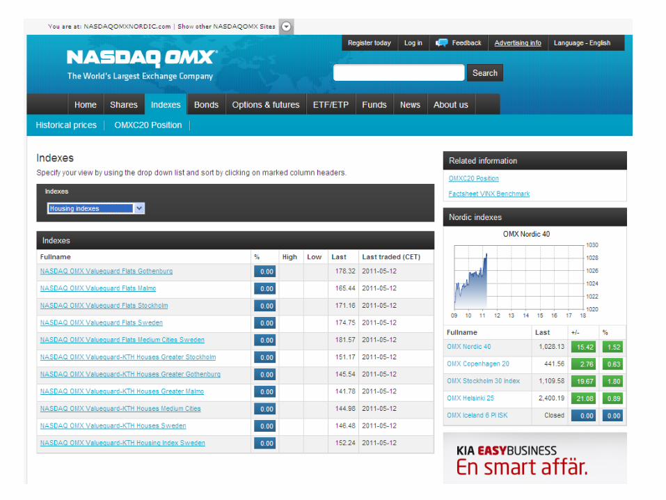
• NasdaqOMX house price index– Insurance/financial products– Complete market

• Thin markets– Geographical or temporal aggregation?

• The objective is to construct house price indexes for all parts of Sweden or at least a large part of the economic value on the single-family housing market.

Literature

• Schwann (1998) – Nearby observation in time

• Englund et al (1999) – Temporal aggregation – not recommended

• McMillen (2003) – Nearby observations in space

• Francke and Vos (2004) – Nearby observations in time and space

Research Procedure

• Estimate hedonic price equation for each region• Perform a cluster analysis– Geographical proximity– Price development– Price level– Price development (2 years)– Combination

• Estimate hedonic price equation for each cluster• Evaluate the performance of the models– R2, MSE

Data

• Single-family houses• 2005-2010• Transaction price, contract date, size, quality,

coordinates

• 100 labor markets (93 with transactions)– Based on potential commuting

No. of transactions per month

1 4 7 10 13 16 19 22 25 28 31 34 37 40 43 46 49 52 55 58 61 64 67 700

100

200

300

400

500

600

Step 1: The Hedonic Price EquationStockholm Västerås Mora

Coefficients t-value Coefficients t-value Coefficients t-valueLiving area 0.3906 85.9 0.4560 25.9 0.3476 6.4Room 2 0.0770 1.6 -0.1475 -1.8 0.1734 1.2Room 3 0.1414 3.0 -0.1105 -1.4 0.3334 2.4Room 4 0.1878 5.9 -0.0501 -0.6 0.3671 2.6Room 5 0.2049 4.3 -0.0329 -0.4 0.3671 3.0Room 6 0.2198 4.6 -0.0087 -0.1 0.4669 3.0Room 7 0.2294 4.8 0.0010 0.0 0.5109 3.3Room 8 0.2377 5.0 0.0458 0.5 0.4315 2.5Room 9 0.2500 5.2 -0.0243 -0.3 0.3167 1.6Room 10 0.2790 5.7 0.0341 0.4 0.7106 3.4Quality index 0.0132 10.9 0.0585 11.7 0.1427 10.4Quality index sq. -0.0001 -7.9 -0.0008 -10.1 -0.0021 -9.3Sea front 0.3829 23.6 0.6049 14.5 0.5272 4.8Sea view 0.0917 19.1 0.0362 2.1 0.1219 3.2Semi-detached -0.0399 -9.8 -0.0449 -3.8 -0.0765 -1.5Detached -0.0634 -12.4 -0.0301 -1.9 -0.1433 -1.4Building period: -1900 0.0711 4.2 0.0451 1.2 0.1806 1.2Building period: 1900-39 -0.0117 -1.5 -0.1432 -5.2 -0.0204 -0.3Building period: 1940-59 -0.0755 -9.3 -0.1442 -5.1 -0.0984 -1.2Building period: 1960-75 -0.0798 -10.0 -0.1286 -4.6 0.0140 0.2Building period: 1976-1990 -0.0278 0.6 -0.0229 -0.8 0.1145 1.4Building period: 1990- 0.0061 0.6 0.0034 0.1 0.4257 3.0Urban -0.0193 -4.1 -0.0293 -1.5 0.1120 3.1R2 0.905 0.880 0.732No of obs. 36158 4633 912No. of obs/month 502 64 13

Temporal AggregationMonth

2005 2006 2007 2008 2009 2010

Västerås Mora

Year

Jan/05

Jun/05

Nov/05

Apr/06

Sep/06

Feb/07Jul/0

7

Dec/07

May/08

Oct/08

Mar/09

Aug/09

Jan/10

Jun/10

Nov/10

80

90

100

110

120

130

140

150

160

170

180

Västerås Mora

Step 2: Cluster AnalysisCluster method

No of clusters

Average no of observations

No of observations in smallest cluster

Average R2

C1 12 18,036 6,909 0.845

C2 9 24,056 9,279 0.812

C3 9 24,049 12,604 0.842

C4 14 15,461 6,066 0.839

C5 11 19,671 8,577 0.846

C6 10 21,646 4,666 0.827

C1: Price developmentC2: Price levelC3: Price development 2 yearC4: Geographical proximityC5: Geographical proximity + Price developmentC6: All

Price development and geographical proximity

Step 3: Evaluation

C1 C2 C3 C4 C5 C6 Total 378,708 376,202 379,272 376,168 376,277 386,112 Large cities 452,149 448,967 450,905 450,140 450,655 466,369 Major regional centre 310,945 308,620 308,984 308,125 307,387 309,730 Minor regional centre 275,900 276,315 297,827 270,041 270,816 274,521 Small regions 186,868 186,938 190,151 186,908 187,846 187,817

C1 C2 C3 C4 C5 C6 Total 375,911 374,277 374,440 373,638 373,718 372641 Large cities 448,025 445,190 446,548 446,144 446,742 444,847 Major regional centre 309,550 308,287 308,084 306,783 305,722 305,419 Minor regional centre 275,197 279,464 273,140 271,680 272,859 273,757 Small regions 192,004 191,565 193,332 190,443 191,523 191,215

Constant implicit prices

Non-constant implicit prices

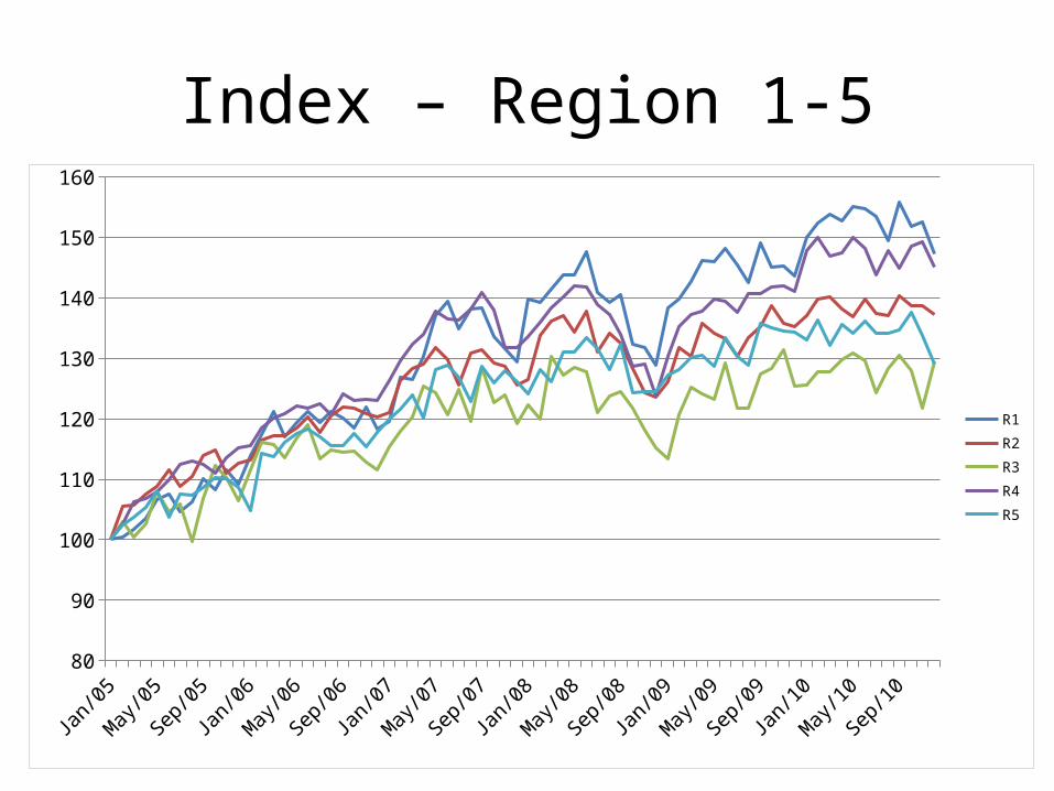
Index – Region 1-5

Jan/05

Apr/05Jul/0

5

Oct/05

Jan/06

Apr/06Jul/0

6

Oct/06

Jan/07

Apr/07Jul/0

7

Oct/07

Jan/08

Apr/08Jul/0

8

Oct/08

Jan/09

Apr/09Jul/0

9

Oct/09

Jan/10

Apr/10Jul/1

0

Oct/10

80

90

100

110

120

130

140

150

160

R1R2R3R4R5

Index – Region 6-10

Jan/05

Apr/05Jul/0

5

Oct/05

Jan/06

Apr/06Jul/0

6

Oct/06

Jan/07

Apr/07Jul/0

7

Oct/07

Jan/08

Apr/08Jul/0

8

Oct/08

Jan/09

Apr/09Jul/0

9

Oct/09

Jan/10

Apr/10Jul/1

0

Oct/10

80

90

100

110

120

130

140

150

160

R6R7R8R9R10

Summary statistics

INDEX R1 R2 R3 R4 R5 R6 R7 R8 R9 R10

average 132 127 120 131 123 121 130 128 123 128

std.dev 16.26 10.39 8.48 13.07 10.25 10.43 13.76 13.79 11.96 11.53Coeff. of variation

0.1230 0.0821 0.0710 0.0997 0.0830 0.0858 0.1059 0.1078 0.0969 0.0903

RETURN

average 0.55% 0.45% 0.36% 0.52% 0.36% 0.22% 0.54% 0.52% 0.47% 0.43%

std.dev 2.73% 2.21% 3.44% 1.99% 2.55% 5.36% 2.75% 2.33% 2.52% 2.70%

Coeff. of variation

5.00 4.97 9.45 3.80 7.11 24.21 5.05 4.46 5.35 6.21

Conclusion

• Thin markets is a problem• It is not obvious how solve it• Temporal and geographical aggregation has been criticized• Especially arbitrary geographical aggregation

• New method how to aggregate in space based on cluster analysis of regions– Price development and geographical proximity

• Out-of-sample test• Other measures to evaluate the method?• Improve the cluster models