constructive newton–puiseux theorem

Thesis for the Degree of Licentiate of Engineering

ConstructiveNewton–Puiseux Theorem

Sheaf Model of the Separable Closure andDynamic Evaluation

Bassel Mannaa

Department of Computer Science and EngineeringUniversity of Gothenburg

Göteborg, Sweden 2014

Constructive Newton–Puiseux TheoremSheaf Model of the Separable Closure and Dynamic Evaluation

Bassel Mannaa

c© 2014 Bassel Mannaa

Technical Report 125LISSN 1652-876XDepartment of Computer Science and EngineeringProgramming Logic Research Group

University of Gothenburg

SE-405 30 GöteborgSwedenTelephone +46 (0)31 786 0000

Printed at Chalmers ReproserviceGöteborg, Sweden 2014

Abstract

Computing the Puiseux expansions of a plane algebraic curve definedby an affine equation over an algebraically closed field is a an importantalgorithm in algebraic geometry. This is the so-called Newton–PuiseuxTheorem. The termination of this algorithm, however, is usually jus-tified by non-constructive means. By adding a separability conditionwe obtain a variant of the algorithm, the termination of which is justi-fied constructively in characteristic 0. Furthermore, we present a pos-sible constructive interpretation of the existence of the separable clo-sure of a field by building, in a constructive metatheory, a suitable sitemodel where there is such separable closure. Consequently, one candispense with the assumption of separable closure and extract compu-tational content from proofs involving this assumption. The theoremof Newton–Puiseux is one example where we use the sheaf model toextract computational content. We then can find Puiseux expansionsof an algebraic curve defined over a non-algebraically closed field K ofcharacteristic 0. The expansions are given as a fractional power seriesover a finite dimensional K-algebra.

Keywords: Newton–Puiseux, Algebraic curve, Sheaf model, Dynamicevaluation, Algebraic number, Grothendieck topos.

i

ii

The present thesis is an extended version of the paper (i) Dy-namic Newton–Puiseux Theorem in “The Journal of Logic andAnalysis” [Mannaa and Coquand, 2013] and the paper (ii) ASheaf Model of the Algebraic Closure in “The Fifth InternationalWorkshop on Classical Logic and Computation" [Mannaaand Coquand, 2014].

Acknowledgments

With thanks to my supervisor Thierry Coquand for his continuingguidance and support. My gratitude to Henri Lombardi and Marie-Françoise Roy for their help and feedback.

iii

Contents

I Constructive Newton–Puiseux Theorem 3

1 Algebraic preliminaries . . . . . . . . . . . . . . . . . . . . 3

2 Newton–Puiseux theorem . . . . . . . . . . . . . . . . . . . 6

3 Related results . . . . . . . . . . . . . . . . . . . . . . . . . . 9

II Categorical Preliminaries 13

1 Functors and presheaves . . . . . . . . . . . . . . . . . . . . 13

2 Elementary topos . . . . . . . . . . . . . . . . . . . . . . . . 14

3 Grothendieck topos . . . . . . . . . . . . . . . . . . . . . . . 15

3.1 Natural numbers object and sheafification . . . . . 16

3.2 Kripke–Joyal sheaf semantics . . . . . . . . . . . . . 16

III Separably Closed Field Extension 19

1 The category of Étale K-Algebras . . . . . . . . . . . . . . . 19

2 A topology for AopK . . . . . . . . . . . . . . . . . . . . . . . 22

3 The separable closure . . . . . . . . . . . . . . . . . . . . . . 26

4 The power series object . . . . . . . . . . . . . . . . . . . . . 30

4.1 The constant sheaves of Sh(AopK , J) . . . . . . . . . . 30

5 Choice axioms . . . . . . . . . . . . . . . . . . . . . . . . . . 35

6 The logic of Sh(AopK , J) . . . . . . . . . . . . . . . . . . . . . 38

7 Eliminating the assumption of algebraic closure . . . . . . 41

IV Dynamic Newton–Puiseux Theorem 43

1 Dynamic Newton–Puiseux Theorem . . . . . . . . . . . . . 43

2 Analysis of the algorithm . . . . . . . . . . . . . . . . . . . 44

v

Introduction

Newton–Puiseux Theorem states that, for an algebraically closed fieldK of zero characteristic, given a polynomial F ∈ K[[X]][Y] there exista positive integer m and a factorization F = ∏n

i=1(Y − ηi) where eachηi ∈ K[[X1/m]][Y]. These roots ηi are called the Puiseux expansions of F.The theorem was first proved by Newton [1736] with the use of Newtonpolygon. Later, Puiseux [1850] gave an analytic proof. It is worth men-tioning that while the proof by Puiseux [1850] deals only with conver-gent power series over the field of complex numbers, the much earlierproof by Newton [1736] was algorithmic in nature and applies to bothconvergent and non-convergent power series [Abhyankar, 1976].

Newton–Puiseux Theorem is usually state as: The field of fractional powerseries (also known as the field of Puiseux series), i.e. the field K〈〈X〉〉 =⋃

m∈Z+ K((X1/m)), is algebraically closed [Walker, 1978].

Abhyankar [1990] presents another proof of this result, the “Shreed-haracharya’s Proof of Newton’s Theorem”. This proof is not construc-tive as it stands. Indeed it assumes decidable equality on the ring K[[X]]of power series over a field, but given two arbitrary power series wecannot decide whether they are equal in finite number of steps. Weexplain in Chapter I how to modify his argument by adding a sepa-rability assumption to provide a constructive proof of the result: Thefield of fractional power series is separably closed. In particular, thetermination of Newton–Puiseux algorithm is justified constructively inthis case. This termination is justified by a non constructive reasoningin most references [Walker, 1978; Duval, 1989; Abhyankar, 1990], withthe exception of [Edwards, 2005]. Following that, we show that the fieldof fractional power series algebraic over K(X) is algebraically closed.

The remainder of this monograph is dedicated to analyzing in a con-structive framework what happens if the field K is not supposed to bealgebraically closed. This is achieved through the method of dynamicevaluation [Della Dora et al., 1985], which replaces factorization by gcdcomputations. The reference [Coste et al., 2001] provides a proof theo-

1

2 Introduction

retic analysis of this method. In Chapter III, we build a sheaf theoreticmodel of dynamic evaluation. The site is given by the category of étalealgebras over the base field with an appropriate Grothendieck topology.We prove constructively that the topos of sheaves on this site containsa separably closed extension of the base field. We also show that incharacteristic 0 the axiom of choice fails to hold in this topos.

With this model we obtain, as presented in Chapter IV, a dynamicversion of Newton–Puiseux theorem, where we compute the Puiseuxexpansions of a polynomial F ∈ K[X, Y] where K is not necessarily al-gebraically closed. The Puiseux expansions in this case are fractionalpower series over an étale K-algebra. We then present a characteriza-tion of the minimal algebra extension of K required for factorization ofF and we show that while there is more than one such minimal exten-sion, any two of them are powers of a common K-algebra.

I

ConstructiveNewton–Puiseux Theorem

A polynomial over a ring is said to be separable if it is coprime with itsderivative. A field K is algebraically closed if any polynomial over K hasa root in K. A field K is separably closed if every separable polynomialover K has a root in K. The goal in this chapter is to prove using onlyconstructive reasoning the statement:

Claim 0.1. For an algebraically closed field K, the field K〈〈X〉〉 of franctionalpower series over K

K〈〈X〉〉 =⋃

m∈Z+

K((X1/m))

is separably closed.

The proof we present is based on a non-constructive proof by Ab-hyankar [1990].

1 Algebraic preliminaries

A (discrete) field is defined to be a non trivial ring in which any elementis 0 or invertible. For a ring R, the formal power series ring R[[X]] is theset of sequences α = α(0) + α(1)X + α(2)X2 + ..., with α(i) ∈ R [Mineset al., 1988].

Definition 1.1 (Apartness). A binary relation R ⊂ S× S on a set S is anapartness if for all x, y, z ∈ S

3

4 I. Constructive Newton–Puiseux Theorem

(i.) ¬xRx.

(ii.) xRy⇒ yRx.

(iii.) xRy⇒ xRz ∨ yRz.

We write x # y to mean xRy where R is an apartness relation on the setof which x and y are elements. As is the case with equality, the set onwhich the apartness is defined it is usually clear from the context . Anapartness is tight if it satisfies ¬x # y⇒ x = y.

Definition 1.2 (Ring with apartness). A ring with apartness is a ring Requipped with an apartness relation # such that

(i.) 0 # 1.

(ii.) x1 + y1 # x2 + y2 ⇒ x1 # x2 ∨ y1 # y2.

(iii.) x1y1 # x2y2 ⇒ x1 # x2 ∨ y1 # y2.

See [Mines et al., 1988; Troelstra and van Dalen, 1988].

Next we define the apartness relation on power series as in [Troelstraand van Dalen, 1988, Ch 8].

Definition 1.3. Let R be a ring with apartness. For α, β ∈ R[[X]] wedefine α # β if ∃n α(n) # β(n).

The relation # on R[[X]] as defined above is an apartness relation andmakes R[[X]] into a ring with apartness [Troelstra and van Dalen, 1988].The relation # on R[[X]] restricts to an apartness relation on the ring ofpolynomials R[X] ⊂ R[[X]].

We note that, if K is a discrete field then for α ∈ K[[X]] we have α # 0iff α(j) is invertible for some j. For F = α0Yn + ... + αn ∈ K[[X]][Y], wehave F # 0 iff αi(j) is invertible for some j and 0 ≤ i ≤ n.

Let R be a commutative ring with apartness. Then R is an integral do-main if it satisfies x # 0∧ y # 0⇒ xy # 0 for all x, y ∈ R. A Heyting fieldis an integral domain satisfying x # 0 ⇒ ∃y xy = 1. The Heyting fieldof fractions of R is the Heyting field obtained by inverting the elementsc # 0 in R and taking the quotient by the appropriate equivalence rela-tion, see [Troelstra and van Dalen, 1988, Ch 8,Theorem 3.12]. For a andb # 0 in R we have a/b # 0 iff a # 0.

For a discrete field K, an element α # 0 in K[[X]] can be written asXm ∑i∈N aiXi with m ∈ N and a0 6= 0. It follows that the ring K[[X]]is an integral domain. If a0 6= 0 we have that ∑i∈N aiXi is invertible in

1. Algebraic preliminaries 5

K[[X]]. We denote by K((X)), the Heyting field of fractions of K[[X]],we also call it the Heyting field of Laurent series over K. Thus anelement apart from 0 in K((X)) can be written as Xn ∑i∈N aiXi witha0 6= 0 and n ∈ Z, i.e. as a series where finitely many terms havenegative exponents.

Unless otherwise qualified, in what follows, a field will always denotea discrete field.

Definition 1.4 (Separable polynomial). Let R be a ring. A polynomialp ∈ R[X] is separable if there exist r, s ∈ R[X] such that rp + sp′ = 1,where p′ ∈ R[X] is the derivative of p.

Lemma 1.5. Let R be a ring and p ∈ R[X] separable. If p = f g then both fand g are separable.

Proof. Let rp + sp′ = 1 for r, s ∈ R[X]. Then r f g + s( f g′ + f ′g) =(r f + s f ′)g + s f g′ = 1, thus g is separable. Similarly for f .

Lemma 1.6. Let R be a ring. If p(X) ∈ R[X] is separable and u ∈ R is aunit then p(uY) ∈ R[Y] is separable.

The following result is usually proved with the assumption that a poly-nomial over a field can be decomposed into irreducible factors. Thisassumption cannot be shown to hold constructively, see [Fröhlich andShepherdson, 1956]. We give a proof without this assumption. It worksover a field of any characteristic.

Lemma 1.7. Let f be a monic polynomial in K[X] where K is a field. If f ′ isthe derivative of f and g monic is the gcd of f and f ′ then writing f = hg wehave that h is separable. We call h the separable associate of f .

Proof. Let a be the gcd of h and h′. We have h = l1a. Let d be the gcd ofa and a′. We have a = l2d and a′ = m2d, with l2 and m2 coprime.

The polynomial a divides h′ = l1a′ + l′1a and hence that a = l2d dividesl1a′ = l1m2d. It follows that l2 divides l1m2 and since l2 and m2 arecoprime, that l2 divides l1.

Also, if an divides p then p = qan and p′ = q′an + nqa′an−1. Hencedan−1 divides p′. Since l2 divides l1, this implies that an = l2dan−1

divides l1 p′. So an+1 divides al1 p′ = hp′.

Since a divides f and f ′, a divides g. We show that an divides g forall n by induction on n. If an divides g we have just seen that an+1

divides g′h. Also an+1 divides h′g since a divides h′. So an+1 dividesg′h + h′g = f ′. On the other hand, an+1 divides f = hg = l1ag. So an+1

divides g which is the gcd of f and f ′.


This implies that a is a unit.

If F is in R[[X]][Y], by FY we mean the derivative of F with respect to Y.

Lemma 1.8. Let K be a field and let F = ∑ni=0 αiYn−i ∈ K[[X]][Y] be sepa-

rable over K((X)), then αn # 0∨ αn−1 # 0

Proof. Since F is separable over K((X)) we have PF + QFY = γ # 0 forP, Q ∈ K[[X]][Y] and γ ∈ K[[X]]. From this we get that γ is equal tothe constant term on the left hand side, i.e. P(0)αn + Q(0)αn−1 = γ # 0.Thus αn # 0∨ αn−1 # 0.

2 Newton–Puiseux theorem

One key of Abhyankar’s proof is Hensel’s Lemma. Here we formu-late a little more general version than the one in [Abhyankar, 1990] bydropping the assumption that the base ring is a field.

Lemma 2.1 (Hensel’s Lemma). Let R be a ring and F(X, Y) = Yn +

∑ni=1 ai(X) Yn−i be a monic polynomial in R[[X]][Y] of degree n > 1. Given

monic non-constant polynomials G0, H0 ∈ R[Y] of degrees r and s respec-tively. Given H∗, G∗ ∈ R[Y] such that F(0, Y) = G0H0, r + s = n andG0H∗ + H0G∗ = 1. We can find G(X, Y), H(X, Y) ∈ R[[X]][Y] of degrees rand s respectively, such that F(X, Y) = G(X, Y)H(X, Y), G(0, Y) = G0 andH(0, Y) = H0.

Proof. The proof is almost the same as Abhyankar’s [Abhyankar, 1990],we present it here for completeness.Since R[[X]][Y] ( R[Y][[X]], we can rewrite F(X, Y) as a power seriesin X with coefficients in R[Y]. Let

F(X, Y) = F0(Y) + F1(Y)X + ... + Fq(Y)Xq + ...

with Fi(Y) ∈ R[Y]. Now we want to find G(X, Y), H(X, Y) ∈ R[Y][[X]]such that F = GH. If we let G = G0 + ∑∞

i=1 Gi(Y)Xi and H = H0 +

∑∞i=1 Hi(Y)Xi, then for each q we need to find Gi(Y), Hj(Y) for i, j ≤ q

such that Fq = ∑i+j=q Gi Hj. We also need deg Gk < r and deg G` < sfor k, ` > 0.We find such Gi, Hj by induction on q. We have that F0 = G0H0. As-sume that for some q > 0 we have found all Gi, Hj with deg Gi < r anddeg Hi < s for 1 ≤ i < q and 1 ≤ j < q. Now we need to find Hq, Gq

2. Newton–Puiseux theorem 7

such that

Fq = G0Hq + H0Gq + ∑i+j=q

i<q,j<q

Gi Hj

We let

Uq = Fq − ∑i+j=q

i<q,j<q

Gi Hj

One can see that deg Uq < n. We are given that G0H∗+ H0G∗ = 1. Mul-tiplying by Uq we get G0H∗Uq + H0G∗Uq = Uq. By Euclidean divisionwe can write UqH∗ = Eq H0 + Hq for some Eq, Hq with deg Hq < s.Thus we write Uq = G0Hq + H0(EqG0 + G∗Uq). One can see thatdeg H0(EqG0 + G∗Uq) < n since deg(Uq − G0Hq) < n. Since H0 ismonic of degree s , deg(EqG0 + G∗Uq) < r. We take Gq = EqG0 + G∗Uq.Now, we can write G(X, Y) and H(X, Y) as monic polynomials in Ywith coefficients in R[[X]], with degrees r and s respectively.

It should be noted that the uniqueness of the factors G and H proven in[Abhyankar, 1990] may not necessarily hold when R is not an integraldomain.

If α = ∑ α(i)Xi is an element of R[[X]] we write m 6 ord α to mean thatα(i) = 0 for i < m and we write m = ord α to mean furthermore thatα(m) is invertible.

Lemma 2.2. Let K be an algebraically closed field of characteristic zero.Let F(X, Y) = Yn + ∑n

i=1 αi(X)Yn−i ∈ K[[X]][Y] be a monic non-constantpolynomial of degree n ≥ 2 separable over K((X)). Then there exist m > 0and a proper factorization F(Tm, Y) = G(T, Y)H(T, Y) with G and H inK[[T]][Y].

Proof. Assume w.l.o.g. that α1(X) = 0. This is Shreedharacharya’s1

trick [Abhyankar, 1990] (a simple change of variable F(X, W − α1/n)).The simple case is if we have ord αi = 0 for some 1 < i ≤ n. Inthis case F(0, Y) = Yn + d2Yn−1 + ... + dn ∈ K[Y] and di 6= 0. Thus∀a ∈ K F(0, Y) 6= (Y− a)n. For any root b of F(0, b) = 0 we have then aproper decomposition F(0, Y) = (Y− b)p H with Y− b and H coprime,and we can use Hensel’s Lemma 2.1 to conclude (In this case we cantake m = 1).

1Shreedharacharya’s trick is also known as Tschirnhaus’s trick [von Tschirnhaus andGreen, 2003]. The technique of removing the second term of a polynomial equation wasalso known to Descartes [Descartes, 1637].


In general, we know by Lemma 1.8 that for k = n or k = n− 1 we haveαk(X) is apart from 0. We then have αk(`) invertible for some `. Wecan then find p and m, 1 < m ≤ n, such that αm(p) is invertible andαi(j) = 0 whenever j/i < p/m. We can then write

F(Tm, TpZ) = Tnp(Zn + c2(T)Zn−2 + · · ·+ cn(T))

with ord cm = 0. As in the simple case, we have a proper decomposition

Zn + c2(T)Zn−2 + · · ·+ cn(T) = G1(T, Z)H1(T, Z)

with G1(T, Z) monic of degree l in Z and H1(T, Z) monic of degree qin Z, with l + q = n, l < n, q < n. We then take

G(T, Y) = TlpG1(T, Y/Tp)

H(T, Y) = TqpH1(T, Y/Tp)

Theorem 2.3. Let K be an algebraically closed field of characteristic zero.Let F(X, Y) = Yn + ∑n

i=1 αi(X)Yn−i ∈ K[[X]][Y] be a monic non-constantpolynomial separable over K((X)). Then there exist a positive integer m andfactorization

F(Tm, Y) =n

∏i=1

(Y− ηi

)ηi ∈ K[[T]]

Proof. If F(X, Y) is separable over K((X)) then F(Tm, Y) for some posi-tive integer m is separable over K((T)). The proof follows directly fromLemma 1.5 and Lemma 2.2 by induction.

Corollary 2.4. Let K be an algebraically closed field of characteristic zero. TheHeyting field of fractional power series over K is separably closed.

Proof. Let F(X, Y) ∈ K((X))[Y] be a monic separable polynomial ofdegree n > 1. Let β # 0 be the product of the denominators of the coef-ficients of F. Then we can write F(X, β−1Z) = β−nG for G ∈ K[[X]][Z].By Lemma 1.6 we get that F, hence G, is separable in Z over K((X)).By Theorem 2.3, G(Tm, Z) factors linearly over K[[T]] for some posi-tive integer m. Consequently we get that F(Tm, Y) factors linearly overK((T)).

3. Related results 9

3 Related results

In the following we show that the elements in K〈〈X〉〉 algebraic overK(X) form a discrete algebraically closed field.

Lemma 3.1. Let K be a field and

F(X, Y) = Yn + b1Yn−1 + ... + bn ∈ K(X)[Y]

be a non-constant monic polynomial such that bn 6= 0. If γ ∈ K((T)) is a rootof F(Tq, Y), then ord γ ≤ d for some positive integer d.

Proof. We can find h ∈ K[X] such that

G = hF = a0(X)Yn + a1(X)Yn−1 + ... + an(X) ∈ K[X][Y]

with an 6= 0. Let d = ord an(Tq). If ord γ > d then so is ord aiγn−i

for 0 ≤ i < n. But we know that in an there is a non-zero term withT-degree d. Thus G(Tq, γ) # 0; Consequently F(Tq, γ) # 0

Note that if α, β ∈ K〈〈X〉〉 are algebraic over K(X) then α + β and αβare algebraic over K(X) [Mines et al., 1988, Ch 6, Corollary 1.4].

Lemma 3.2. Let K be a field. The set of elements in K〈〈X〉〉 algebraic overK(X) is a discrete set; More precisely # is decidable on this set.

Proof. It suffices to show that for an element γ in this set γ # 0 isdecidable. Let F = Yn + a1(X)Yn−1 + ... + an ∈ K(X)[Y] be a monicnon-constant polynomial. Let γ ∈ K((T)) be a root of F(Tq, Y). IfF = Yn then ¬γ # 0. Otherwise, F can be written as Ym(Yn−m + ...+ am)with 0 ≤ m < n and am 6= 0. By Lemma 3.1 we can find d such thatany element in K((T)) that is a root of Yn−m + ...+ am has an order lessthan or equal to d. Thus γ # 0 if an only if ord γ ≤ d.

If α # 0 ∈ K〈〈X〉〉 is algebraic over K(X) then 1/α is algebraic overK(X). Thus the set of elements in K〈〈X〉〉 algebraic over K(X) form afield K〈〈X〉〉alg ⊂ K〈〈X〉〉. This field is in fact algebraically closed inK〈〈X〉〉 [Mines et al., 1988, Ch 6, Corollary 1.5].

Since for an algebraically closed field K we have shown K〈〈X〉〉 to beonly separably algebraically closed, we need a stronger argument toshow that K〈〈X〉〉alg is algebraically closed.

Lemma 3.3. For an algebraically closed field K of characteristic zero, the fieldK〈〈X〉〉alg is algebraically closed.


Proof. Let F ∈ K〈〈X〉〉alg[Y] be a monic non-constant polynomial of de-gree n. By Lemma 3.2 K〈〈X〉〉alg is a discrete field. By Lemma 1.7we can decompose F as F = HG with H ∈ K〈〈X〉〉alg[Y] a non-constantmonic separable polynomial. By Corollary 2.4, H has a root η in K〈〈X〉〉.Since K〈〈X〉〉alg is algebraically closed in K〈〈X〉〉 we have that η ∈K〈〈X〉〉alg.

We can draw similar conclusions in the case of real closed fields 2.

Lemma 3.4. Let R be a real closed field. Then

(i.) For any α # 0 ∈ R〈〈X〉〉 we can find β ∈ R〈〈X〉〉 such that β2 = αor −β2 = α.

(ii.) A separable monic polynomial of odd degree in R〈〈X〉〉[Y] has a rootin R〈〈X〉〉.

Proof. Since R is real closed, the first statement follows from the fact anelement a0 + a1X + ... ∈ R[[X]] with a0 > 0 has a square root in R[[X]].

Let F(X, Y) = Yn + α1Yn−1 + ... + αn ∈ R[[X]][Y] be a monic poly-nomial of odd degree n > 1 separable over R((X)). We can assumew.l.o.g. that α1 = 0. Since F is separable, i.e. PF + QFY = 1 for someP, Q ∈ R((X))[Y], then by a similar construction to that in Lemma 2.2we can write F(Tm, TpZ) = TnpV for V ∈ R[[T]][Z] such that V(0, Z) 6=(Z + a)n for all a ∈ R. Since R is real closed and V(0, Z) has odd de-gree, V(0, Z) has a root r in R. We can find proper decomposition intocoprime factors V(0, Z) = (Z − r)`q. By Hensel’s Lemma 2.1, we liftthose factors to factors of V in R[[T]][Z] thus we can write F = GH formonic non-constant G, H ∈ R[[T]][Y]. By Lemma 1.5 both G and H areseparable. Either G or H has odd degree. Assuming G has odd degreegreater than 1, we can further factor G into non-constant factors. Thestatement follows by induction.

Let R be a real closed field. By Lemma 3.2 we see that R〈〈X〉〉alg isdiscrete. A non-zero element in α ∈ R〈〈X〉〉alg can be written α =Xm/n(a0 + a1X1/n + ...) for n > 0, m ∈ Z with a0 6= 0. Then α is positiveiff its initial coefficient a0 is positive [Basu et al., 2006]. We can then seethat this makes R〈〈X〉〉alg an ordered field.

Lemma 3.5. For a real closed field R, the field R〈〈X〉〉alg is real closed.

Proof. Let α ∈ R〈〈X〉〉alg. Since R〈〈X〉〉alg is discrete, by Lemma 3.4 wecan find β ∈ R〈〈X〉〉alg such that β2 = α or −β2 = α.

2We reiterate that by a field we mean a discrete field.

3. Related results 11

Let F ∈ R〈〈X〉〉alg[Y] be a monic polynomial of odd degree n. ApplyingLemma 1.7 several times, by induction we have F = H1H2..Hm withHi ∈ R〈〈X〉〉alg[Y] separable non-constant monic polynomial. For somei we have Hi of odd degree. By Lemma 3.4, Hi has a root in R〈〈X〉〉alg.Thus F has a root in R〈〈X〉〉alg.

II

Categorical Preliminaries

In this chapter we give a brief outline of some of the notions and resultsthat will be used in Chapter III. We assume that the reader is familiarwith basic notions from category theory used in general algebra.

1 Functors and presheaves

A (covariant) functor F : C → D between two categories C and D assignsto each object C of C an object F(C) of D and to each arrow f : C → Bof C an arrow F( f ) : F(C) → F(B) of D such that F(1C) = 1F(C) andF( f g) = F( f )F(g). A natural transformation Θ between two functorsF : C → D and G : C → D is collection of arrows, indexed by objects ofC, of the form ΘC : F(C) → G(C) such that for each arrow f : C → A

of C the diagram

F(C) G(C)

F(A) G(A)

F( f )

ΘC

G( f )

ΘA

commutes.

A contravariant functor G between C and D is a covariant functor G :Cop → D. Thus for f : C → B of C we have G( f ) : G(B) → G(C)in D and G( f g) = G(g)G( f ). The collection of functors between twocategories C and D and natural transformation between them form acategory DC .

A functor F ∈ SetCop

is called a presheaf of sets over/on the category C.For an arrow f : A → B of C the map F( f ) : F(B) → F(A) is called arestriction map between the sets F(B) and F(A). An element x ∈ F(B)

13

14 II. Categorical Preliminaries

has a restriction x f = (F( f ))(x) ∈ F(A) called the restriction of x alongf .

A category is small if the collection of objects in the category form aset. A category is locally small if the collection of morphisms betweenany two objects in the category is a set. The presheaf yC := Hom(−, C)of SetC

opassociates to each object A of C the set Hom(A, C) of arrows

A→ C of C. Let g ∈ yC(B) and let f : A→ B be a morphism of C theng f ∈ yC(A) is the restriction of g along f . The presheaf yC is called theYoneda embedding of C.

Fact 1.1 (Yoneda Lemma). Let C be a locally small category and F ∈ SetCop

.We have an isomorphism Nat(yC, F) ∼= F(C). Where Nat(yC, F) is the set ofnatural transformations Hom

SetCop (yC, F) between the presheaves yC and F.

A sieve S on an object C of a small category C is a set of morphisms withcodomain C such that if f : D → C ∈ S then for any g with codomainD we have f g ∈ S. Given a set S of morphisms with codomain C wedefine the sieve generated by S to be (S) = f g | f ∈ S, cod(g) =dom( f ). Note that in SetC

opa sieve uniquely determines a subobject

of yC. Given f : D → C and S a collection of arrows with codomain Cthen f ∗(S) = g | cod(g) = D, f g ∈ S. When S is a sieve f ∗(S) = S fis a sieve on D, the restriction of S along f in SetC

op. Dually, given

g : C → D and M a collection of arrows with domain C then g∗(M) =h | dom(h) = D, hg ∈ M. The presheaf Ω is the presheaf assigning toeach object C the set Ω(C) of sieves on C with restriction maps f ∗ foreach morphism f : D → C of C.

2 Elementary topos

An elementary topos [Lawvere, 1970] is a category C such that

1. C has all finite limits and colimits.

2. C is cartesian closed. In particular for any two objects C and D ofC there is an object DC such that there is a one-to-one correspon-dence between the arrows A → DC and the arrows A× C → Dfor any object A of C. For a locally small category this is expressedas Hom(A× C, D) ∼= Hom(A, DC).

3. C has a subobject classifier. That is, there is an object Ω and a map

1 Ωtrue such that for any object C of C there is a one-to-one

3. Grothendieck topos 15

correspondence between the subobjects of C given by monomor-phisms with codomain C and the maps from C to Ω (called clas-sifying/characteristic maps). A subobject is uniquely determined

by the pullback of the map 1 Ωtrue along the characteristicmap.

An elementary topos can be considered as a generalization of the cate-gory Set of sets. The category SetC

opof presheaves on a small category

C is an elementary topos. The lattice of subobjects of an object C in anelementary topos E (monomorphisms with codomain C) is a Heytingalgebra.

3 Grothendieck topos

In this section we define the notions of site, coverage, and sheaf follow-ing [Johnstone, 2002b,a].

Definition 3.1 (Coverage). By a coverage on a category C we mean afunction J assigning to each object C of C a collection J(C) of familiesof morphisms of the form fi : Ci → C | i ∈ I such that :If fi : Ci → C | i ∈ I ∈ J(C) and g : D → C is a morphism, thenthere exist hj : Dj → D | j ∈ J ∈ J(D) such that for any j ∈ J we haveghj = fik for some i ∈ I and some k : Dj → Ci.

A site (C, J) is a small category C equipped with a coverage J. A family fi : Ci → C | i ∈ I ∈ J(C) is called elementary cover or elementarycovering family of C.

Definition 3.2 (Compatible family). Let C be a category and F : Cop →Set a presheaf. Let fi : Ci → C | i ∈ I be a family of morphisms in C.A family si ∈ F(Ci) | i ∈ I is compatible if for all `, j ∈ I wheneverwe have g : D → C` and h : D → Cj satisfying f`g = f jh we haveF(g)(s`) = F(h)(sj).

Definition 3.3 (The sheaf axiom). Let C be a category. A presheaf F :Cop → Set satisfies the sheaf axiom for a family of morphisms fi :Ci → C | i ∈ I if whenever si ∈ F(Ci) | i ∈ I is a compatiblefamily then there exist a unique s ∈ F(C) restricting to si along fi for alli ∈ I. That is to say when there exist a unique s such that for all i ∈ I,F( fi)(s) = si. One usually refers to s as the amalgamation of sii∈I .

Let (C, J) be a site. A presheaf F ∈ SetCop

is a sheaf on (C, J) if it satisfiesthe sheaf axiom for each object C of C and each family of morphisms inJ(C), i.e. if it satisfies the sheaf axiom for elementary covers.


The category of sheaves on a small site Sh(C, J) is an elementary topos.

3.1 Natural numbers object and sheafification

A natural numbers object in a category with a terminal object is anobject N along with two morphisms z : 1 → N and s : N → N such

that for any diagram of the form 1 C Cf g

there is aunique morphism h : N → C making the diagram below commute.

C C

1 N N

g

f

z

h

s

h

Fact 3.4. In SetCop

the constant presheaf N such that N(C) = N andN( f ) = 1N for every object C and morphism f of C is a natural numbersobject.

Let (C, J) be a site. The sheaf topos Sh(C, J) is a full subcategory of thepresheaf category SetC

op. By the sheafification of a presheaf P ∈ SetC

op

we mean a sheaf P of Sh(C, J) along with a presheaf morphism Γ : P→P such that for any sheaf E and any presheaf morphism Λ : P → Ethere is a unique sheaf morphism ∆ : P → E making the following

diagram commute.

P E

P

Λ

Γ∆

Fact 3.5. Let (C, J) be a site. The sheaf topos Sh(C, J) contains a naturalnumbers object N where N is the sheafification of the natural numbers presheafN.

3.2 Kripke–Joyal sheaf semantics

We work with a typed language with equality L[V1, ..., Vn] having thebasic types V1, ..., Vn and type formers − × −, (−)−,P(−). The lan-guage L[V1, ..., Vn] has typed constants and function symbols. For anytype Y one has a stock of variables y1, y2, ... of type Y. Terms and for-mulas of the language are defined as usual. We work within the prooftheory of intuitionistic higher-order logic (IHOL). A detailed descrip-tion of this deduction system is given in [Awodey, 1997].

3. Grothendieck topos 17

The language L[V1, ..., Vn] along with deduction system IHOL can beinterpreted in an elementary topos in what is referred to as topos se-mantics. For a sheaf topos this interpretation takes a simpler form remi-niscent of Beth semantics, usually referred to as Kripke–Joyal sheaf seman-tics. We describe this semantics here briefly following [Šcedrov, 1984].Let E = Sh(C, J) be a sheaf topos. First we define a closure J∗ of J asfollows.

Definition 3.6 (Closure of a coverage).

(i.) C 1c−→ C ∈ J∗(C) for all objects C in C.

(ii.) If Cifi−→ Ci∈I ∈ J(C) then Ci

fi−→ Ci∈I ∈ J∗(C).

(iii.) If Cifi−→ Ci∈I ∈ J∗(C) and for each i ∈ I we have Cij

gij−→

Cij∈Ji ∈ J∗(Ci) then Cijfi gij−−→ Ci∈I,j∈Ji ∈ J∗(C).

An family S ∈ J∗(C) is called cover or covering family of C.

An interpretation of the language L[V1, ..., Vn] in the topos E is givenas follows: Associate to each basic type Vi of L[V1, ..., Vn] an objectVi of E . If Y and Z are types of L[V1, ..., Vn] interpreted by objects Yand Z, respectively, then the types Y × Z, YZ,P(Z) are interpreted byY× Z, YZ, ΩZ, respectively, where Ω is the subobject classifier of E . Aconstant e of type E is interpreted by an arrow 1 e−→ E where E is theinterpretation of E. For a term τ and an object X of E , we write τ : X tomean τ has a type X interpreted by the object X.

Let φ(x1, ..., xn) be a formula with variables x1 : X1, ..., xn : Xn. Letc1 ∈ Xj(C), ..., cn ∈ Xn(C) for some object C of C. We define the re-lation C forces φ(x1, ..., xn)[c1, ..., cn] written C φ(x1, ..., xn)[c1, ..., cn] byinduction on the structure of φ.

Definition 3.7 (Forcing). First we replace the constants in φ by variablesof the same type as follows: Let e1 : E1, ..., em : Em be the constants inφ(x1, ..., xn) then C φ(x1, ..., xn)[c1, ..., cn] iff

C φ[y1/e1, ..., ym/em](y1, ..., ym, x1, ..., xn)[e1C (∗), ..., emC (∗), c1, ..., cn]

where yi : Ei and ei : 1→ Ei is the interpretation of ei.

Now it suffices to define the forcing relation for formulas free of con-stants by induction as follows:

> C >.


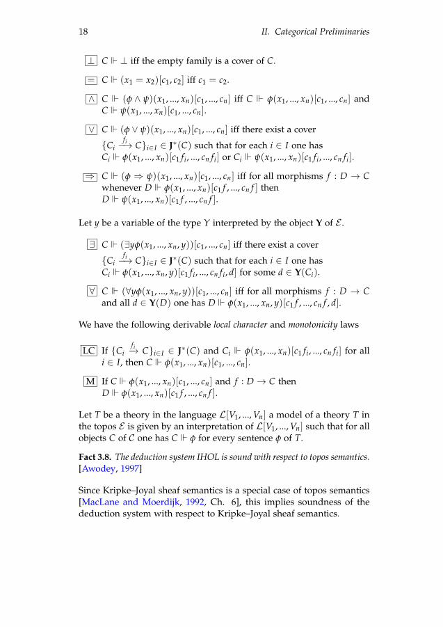
⊥ C ⊥ iff the empty family is a cover of C.

= C (x1 = x2)[c1, c2] iff c1 = c2.

∧ C (φ ∧ ψ)(x1, ..., xn)[c1, ..., cn] iff C φ(x1, ..., xn)[c1, ..., cn] andC ψ(x1, ..., xn)[c1, ..., cn].

∨ C (φ ∨ ψ)(x1, ..., xn)[c1, ..., cn] iff there exist a cover

Cifi−→ Ci∈I ∈ J∗(C) such that for each i ∈ I one has

Ci φ(x1, ..., xn)[c1 fi, ..., cn fi] or Ci ψ(x1, ..., xn)[c1 fi, ..., cn fi].

⇒ C (φ ⇒ ψ)(x1, ..., xn)[c1, ..., cn] iff for all morphisms f : D → Cwhenever D φ(x1, ..., xn)[c1 f , ..., cn f ] thenD ψ(x1, ..., xn)[c1 f , ..., cn f ].

Let y be a variable of the type Y interpreted by the object Y of E .

∃ C (∃yφ(x1, ..., xn, y))[c1, ..., cn] iff there exist a cover

Cifi−→ Ci∈I ∈ J∗(C) such that for each i ∈ I one has

Ci φ(x1, ..., xn, y)[c1 fi, ..., cn fi, d] for some d ∈ Y(Ci).

∀ C (∀yφ(x1, ..., xn, y))[c1, ..., cn] iff for all morphisms f : D → Cand all d ∈ Y(D) one has D φ(x1, ..., xn, y)[c1 f , ..., cn f , d].

We have the following derivable local character and monotonicity laws

LC If Cifi−→ Ci∈I ∈ J∗(C) and Ci φ(x1, ..., xn)[c1 fi, ..., cn fi] for all

i ∈ I, then C φ(x1, ..., xn)[c1, ..., cn].

M If C φ(x1, ..., xn)[c1, ..., cn] and f : D → C thenD φ(x1, ..., xn)[c1 f , ..., cn f ].

Let T be a theory in the language L[V1, ..., Vn] a model of a theory T inthe topos E is given by an interpretation of L[V1, ..., Vn] such that for allobjects C of C one has C φ for every sentence φ of T.

Fact 3.8. The deduction system IHOL is sound with respect to topos semantics.[Awodey, 1997]

Since Kripke–Joyal sheaf semantics is a special case of topos semantics[MacLane and Moerdijk, 1992, Ch. 6], this implies soundness of thededuction system with respect to Kripke–Joyal sheaf semantics.

III

Separably Closed FieldExtension

In Section 1 we describe the category AK of étale K-algebras. In Sec-tion 2 we specify a coverage J on the category Aop

K . In Section 3 wedemonstrate that the topos Sh(Aop

K , J) contains a separably closed ex-tension of K. In Section 5 and Section 6 we look at the logical propertiesof the topos Sh(Aop

K , J) with respect to choice axioms and booleanness.

1 The category of Étale K-Algebras

We recall the definition of separable polynomial from Chapter I.

Definition 1.1 (Separable polynomial). Let R be a ring. A polynomialp ∈ R[X] is separable if there exist r, s ∈ R[X] such that rp + sp′ = 1,where p′ ∈ R[X] is the derivative of p.

Let K be a discrete field and A a K-algebra. An element a ∈ A is sep-arable algebraic if it is the root of a separable polynomial over K. Thealgebra A is separable algebraic if all elements of A are separable alge-braic. An algebra over a field is said to be finite if it has finite dimensionas a vector space over K. We note that if A is a finite K-algebra then wehave a finite basis of A as a vector space over K.

Definition 1.2. An algebra A over a field K is étale if it is finite andseparable algebraic.

It is worth mentioning that there is an elementary characterization ofétale K-algebras given as follows: Let A be a finite K-algebra with basis

19

20 III. Separably Closed Field Extension

(a1, ..., an). We associate to each element a ∈ A the matrix representa-tion [ma] ∈ M(n, K) of the K-linear map x 7→ ax. Let TrA/K(a) be thetrace of [ma]. Let discA/K(x1, ...., xn) = det((TrA/K(xixj))1≤i,j≤n). Thealgebra A is étale if discA/K(a1, ..., an) is a unit. The equivalence be-tween Definition 1.2 and this characterization is shown in [Lombardiand Quitté, 2011, Ch. 6, Theorem 1.7].

Definition 1.3 (Regular ring). A commutative ring R is (von Neumann)regular if for every element a ∈ R there exist b ∈ R such that aba = aand bab = b. This element b is called the quasi-inverse of a.

The quasi-inverse b of an element a is unique for a [Lombardi andQuitté, 2011, Ch 4]. We thus use the notation a∗ to refer to the quasi-inverse of a. A ring is regular iff it is zero-dimensional, i.e. any primeideal is maximal, and reduced, i.e. an = 0⇒ a = 0. To be von Neumannregular is equivalent to the fact that any principal ideal (and henceany finitely generated ideal) is generated by an idempotent. If a isan element in R then the element e = aa∗ is an idempotent such that〈e〉 = 〈a〉 and R is isomorphic to R0 × R1 with R0 = R/〈e〉 and R1 =R/〈1− e〉. Furthermore a is 0 on the component R0 and invertible onthe component R1.

Definition 1.4 (Fundamental system of orthogonal idempotents). Afamily (ei)i∈I of idempotents in a ring R is a fundamental system oforthogonal idempotents if ∑i∈I ei = 1 and ∀i, j[i 6= j⇒ eiej = 0].

Lemma 1.5. Given a fundamental system of orthogonal idempotents (ei)i∈Iin a ring A we have a decomposition A ∼= ∏i∈I A/〈1− ei〉.

Proof. Follows directly by induction from the fact that A ∼= A/〈e〉 ×A/〈1− e〉 for an idempotent e ∈ A.

Fact 1.6.

1. An étale algebra over a field K is zero-dimensional and reduced, i.e.regular.

2. Let A be a finite K-algebra and (ei)i∈I a fundamental system of orthog-onal idempotents of A. Then A is étale if and only if A/〈1− ei〉 is étalefor each i ∈ I.

[Lombardi and Quitté, 2011, Ch 6, Fact 1.3].

Note that an étale K-algebra A is finitely presented, i.e. can be writtenas K[X1, ..., Xn]/〈 f1, ..., fm〉.We define strict Bézout rings as in [Lombardi and Quitté, 2011, Ch 4].

1. The category of Étale K-Algebras 21

Definition 1.7. A ring R is a (strict) Bézout ring if for all a, b ∈ R wecan find g, a1, b1, c, d ∈ R such that a = a1g, b = b1g and ca1 + db1 = 1.

If R is a regular ring then R[X] is a strict Bézout ring (and the converseis true [Lombardi and Quitté, 2011]). Intuitively we can compute thegcd as if R was a field, but we may need to split R when deciding ifan element is invertible or 0. Using this, we see that given a, b in R[X]we can find a decomposition R1, . . . , Rn of R and for each i we haveg, a1, b1, c, d in Ri[X] such that a = a1g, b = b1g and ca1 + db1 = 1 withg monic. The degree of g may depend on i.

Lemma 1.8. If A is an étale K-algebra and p in A[X] is a separable polynomialthen A[a] = A[X]/〈p〉 is an étale K-algebra.

Proof. See [Lombardi and Quitté, 2011, Ch 6, Lemma 1.5].

By a separable extension of a ring R we mean a ring R[a] = R[X]/〈p〉where p ∈ R[X] is non-constant, monic and separable.

In order to build the classifying topos of a coherent theory T it is cus-tomary in the literature to consider the category of all finitely presentedT0 algebras where T0 is an equational subtheory of T. The axioms of Tthen give rise to a coverage on the dual category [Makkai and Reyes,1977, Ch. 9]. For our purpose consider the category C of finitely pre-sented K-algebras. Given an object R of C, the axiom schema of separa-ble closure and the field axiom give rise to families

(i.) R→ R[X]/〈p〉 where p ∈ R[X] is monic and separable.

(ii.)

R/〈a〉

R

R[ 1a ]

, for a ∈ R.

Dualized, these are covering families of R in Cop. We observe howeverthat we can limit our consideration only to étale K-algebras. In this casewe can assume a is an idempotent.

We study the small category AK of étale K-algebras over a fixed field Kand K-homomorphisms. First we fix an infinite set of names S. Anobject of AK is an étale algebra of the form K[X1, ..., Xn]/〈 f1, ..., fm〉where Xi ∈ S for all 1 ≤ i ≤ n. Note that for each object R, there is aunique morphism K → R. If A and B are objects of AK and ϕ : A → B


is a morphism of AK, the diagramK

A Bϕ

commutes.The

trivial ring 0 is the terminal object in the category AK and K is its initialobject.

2 A topology for AopK

Next we specify a coverage J on the category AopK per Definition II.3.1.

A coverage is specified by a collection J(A) of families of morphismsof Aop

K with codomain A for each object A. Rather than describing thecollection J(A) directly, we define for each object A a collection Jop(A)of families of morphisms of AK with domain A. Then we take J(A)to be the dual of Jop(A) in the sense that for any object A we haveϕi : Ai → Ai∈I ∈ J(A) if and only if ϕi : A→ Aii∈I ∈ Jop(A) wherethe morphism ϕi of AK is the dual of the morphism ϕi of Aop

K . We callJop cocoverage and elements of Jop(A) elementary cocovers (elementarycocovering families) of A. Analogously we define the closure J∗op tobe the dual of the closure J∗(See Definition II.3.6). We call a familyT ∈ J∗op(A) a cocover (cocovering family) of A.

Definition 2.1 (Topology for AopK ). Let A be an object of AK.

(i.) If (ei)i∈I is a fundamental system of orthogonal idempotents ofA, then

Aϕi−−→ A/〈1− ei〉i∈I ∈ Jop(A)

where for each i ∈ I, ϕi is the canonical homomorphism.

(ii.) Let A[a] be a separable extension of A. We have

Aψ−→ A[a] ∈ Jop(A)

where ψ is the canonical homomorphism.

Note that in particular 2.1.(i.) implies that the trivial algebra 0 is cov-ered by the empty family of morphisms since an empty family of el-ements in this ring form a fundamental system of orthogonal idem-potents (The empty sum equals 0 = 1 and the empty product equals

1 = 0). Also note that 2.1.(ii.) implies that A1A−−→ A ∈ Jop(A).

Lemma 2.2. The collections J of Definition 2.1 is a coverage on AopK .

2. A topology for AopK 23

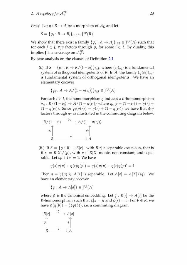
Proof. Let η : R→ A be a morphism of AK and let

S = ϕi : R→ Rii∈I ∈ Jop(R)

We show that there exist a family ψj : A → Ajj∈J ∈ Jop(A) such thatfor each j ∈ J, ψjη factors through ϕi for some i ∈ I. By duality, thisimplies J is a coverage on Aop

K .

By case analysis on the clauses of Definition 2.1

(i.) If S = ϕi : R→ R/〈1− ei〉i∈I , where (ei)i∈I is a fundamentalsystem of orthogonal idempotents of R. In A, the family (η(ei))i∈Iis fundamental system of orthogonal idempotents. We have anelementary cocover

ψi : A→ A/〈1− η(ei)〉i∈I ∈ Jop(A)

For each i ∈ I, the homomorphism η induces a K-homomorphismηei : R/〈1− ei〉 → A/〈1− η(ei)〉 where ηei (r + 〈1− ei〉) = η(r) +〈1− η(ei)〉. Since ψi(η(r)) = η(r) + 〈1− η(ei)〉 we have that ψiηfactors through ϕi as illustrated in the commuting diagram below.

R/〈1− ei〉 A/〈1− η(ei)〉

R A

ηei

ϕi

η

ψi

(ii.) If S = ϕ : R → R[r] with R[r] a separable extension, that isR[r] = R[X]/〈p〉, with p ∈ R[X] monic, non-constant, and sepa-rable. Let sp + tp′ = 1. We have

η(s)η(p) + η(t)η(p′) = η(s)η(p) + η(t)η(p)′ = 1

Then q = η(p) ∈ A[X] is separable. Let A[a] = A[X]/〈q〉. Wehave an elementary cocover

ψ : A→ A[a] ∈ Jop(A)

where ψ is the canonical embedding. Let ζ : R[r] → A[a] be theK-homomorphism such that ζ|R = η and ζ(r) = a. For b ∈ R, wehave ψ(η(b)) = ζ(ϕ(b)), i.e. a commuting diagram

R[r] A[a]

R A

ζ

ϕ

η

ψ


Lemma 2.3. Let P : AK → Set be a presheaf on AopK such that P(0) = 1.

Let R be an object of AK and let (ei)i∈I be a fundamental system of orthogonalidempotents of R. For each i ∈ I, let Ri = R/〈1− ei〉 and let ϕi : R → Ribe the canonical homomorphism. Any family si ∈ P(Ri) is a compatiblefamily with respect to the family morphisms ϕi : R→ Rii∈I .

Proof. For i, j ∈ I, let B be an object and let ϑ : Ri → B and ψ : Rj → Bbe two morphisms such that ϑϕi = ψϕj, i.e. we have a commuting

diagram

R/〈1− ei〉 B

R R/〈1− ej〉

ϑ

ϕi

ϕj

ψ

We will show that P(ϑ)(si) = P(ψ)(sj).

(i.) If i = j, then since ϕi is surjective we have ϑ = ψ and P(ϑ) =P(ψ).

(ii.) If i 6= j, then since eiej = 0, ϕi(ei) = 1 and ϕj(ej) = 1 we haveϕj(eiej) = ϕj(ei) = 0. But then

1 = ϑ(1) = ϑ(ϕi(ei)) = ψ(ϕj(ei)) = ψ(0) = 0

Hence B is the trivial algebra 0. By assumption P(0) = 1, henceP(ϑ)(si) = P(ψ)(sj) = ∗.

Corollary 2.4. Let F be a sheaf on (AopK , J). Let R be an object of AK and

(ei)i∈I a fundamental system of orthogonal idempotents of R. Let Ri =R/〈1 − ei〉 and ϕi : R → Ri be the canonical homomorphism. The mapf : F(R)→ ∏i∈I F(Ri) such that f (s) = (F(ϕi)s)i∈I is an isomorphism.

Proof. Since F(0) = 1, by Lemma 2.3 any family of elements of the formsi ∈ F(Ri) | i ∈ I is compatible. Since F is a sheaf satisfying thesheaf axiom II.3.3, the family si ∈ F(Ri)i∈I has a unique amalgama-tion s ∈ F(R) with restrictions sϕi = si. The isomorphism is given byf s = (sϕi)i∈I . We can then use the tuple notation (si)i∈I to denote theelement s in F(R).

One say that a polynomial f ∈ R[X] has a formal degree n if f can bewritten as f = anXn + ... + a0 which is to express that for any m > n

2. A topology for AopK 25

the coefficient of Xm is known to be 0. One, on the other hand, say thata polynomial f has a degree n > 0 if f has a formal degree n and thecoefficient of Xn is not 0.

Lemma 2.5. Let R be a regular ring and p1, p2 ∈ R[X] be monic polynomialsof degrees n1 and n2 respectively. Let R[a, b] = R[X, Y]/〈p1(X), p2(Y)〉. Letq1, q2 ∈ R[Z] be of formal degrees m1 < n1 and m2 < n2 respectively. Ifq1(a) = q2(b) then q1 = q2 = r ∈ R.

Proof. Let q1(a) = q2(b), then in R[X, Y]

q1(X)− q2(Y) = f (X, Y)p1(X) + g(X, Y)p2(Y)

for some f , g ∈ R[X, Y].

In R[a][Y] = R[X, Y]/〈p1(X)〉 we have q1(a) − q2(Y) = g(a, Y)p2(Y).But p2(Y) is monic of Y-degree n2 while q2(Y) − q1(a) has formal Y-degree m2 < n2, hence, the coefficients of g(a, Y) ∈ R[a][Y] are all equalto 0 in R[a]. We have then that all coefficient of Y` with ` > 0 in q2(Y)are equal 0. That is, q2 = r ∈ R and that q1(a) is equal to the constantcoefficient r of q2(Y). Thus in R[X] we have q1(X)− r = h(X)p1(X) forsome h ∈ R[X]. Similarly, since (q1(X)− r) has a formal X-degree m1and p1 is monic of degree n1 > m1 we get that q1 = r ∈ R.

Corollary 2.6. Let R be an object of AK and p ∈ R[X] separable and monic.Let R[a] = R[X]/〈p〉 and ϕ : R → R[a] the canonical morphism. LetR[b, c] = R[X, Y]/〈p(X), p(Y)〉. The commuting diagram

R[a] R[b, c]

R R[a]

ϑ

ϕ

ϕ

ζ ϑ|R(r) = ζ|R(r) = r, ϑ(a) = b, ζ(a) = c

is a pushout diagram of AK. Moreover, ϕ is the equalizer of ζ and ϑ.

Proof. Let R[a] Bη

ψbe morphisms of AK such that

ηϕ = ψϕ. Then for all r ∈ R we have η(r) = ψ(r).Let γ : R[c, d]→ B be the homomorphism such that γ(r) = η(r) = ψ(r)for all r ∈ R while γ(b) = η(a), γ(c) = ψ(a). Then γ is the uniquemap such that γϑ = η and γζ = ψ and we have proved that the abovediagram is a pushout diagram.

Let A be an object of AK and let $ : A → R[a] be a map such thatζ$ = ϑ$. By Lemma 2.5 if for f ∈ R[a] one has ζ( f ) = ϑ( f ) then f ∈ R


(i.e. f is of degree 0 as a polynomial in a over R). Thus $(A) ⊂ R and wecan factor $ uniquely (since ϕ is injective) as $ = ϕη for η : A→ R.

Now let ϕ : R → R[a] be a singleton elementary cocover. Sinceone can form the pushout of ϕ with itself, the compatibility conditionon a singleton family s ∈ P(R[a]) can be simplified as follows : Let

R R[a] Aϕ η

ϑbe a pushout diagram. A family s ∈ P(R[a])

is compatible if and only if sϑ = sη.

Corollary 2.7. The coverage J is subcanonical. That is, all representablepresheaves are sheaves on (Aop

K , J).

Proof. Consider the presheaf yA = HomAK (A,−) for some object A ofAop

K .

(i.) Given (ei)i∈I a fundamental system of orthogonal idempotents,an elementary cocover ϕi : R → R/〈1 − ei〉i∈I ∈ Jop(R) anda family ηi : A → R/〈1 − ei〉i∈I . By the isomorphism R ∼=∏i∈I R/〈1− ei〉 there is a unique η : A→ R such that ϕiη = ηi.

(ii.) Let R[a] be a separable extension of R. Consider the elemen-

tary cocover R ϕ−→ R[a] ∈ Jop(R) and let Aψ−→ R[a] be a

compatible family. By Corollary 2.6, one has a pushout diagram

R R[a] R[b, c]ϕ ϑ

ζ. Compatibility implies that ϑψ =

ζψ. But by Corollary 2.6 the canonical embedding ϕ is the equal-

izer of ϑ and ζ. Thus there exist a unique Aη−→ R ∈ yA(R) such

that ϕη = ψ.

The terminal object in the category Sh(AopK , J) is the sheaf sending each

object to the set ∗ = 1. This is the sheaf yK since in AopK there is only

one morphism between any object and the object K.

3 The separable closure

We define the presheaf F : AK → Set to be the forgetful functor. Thatis, for an object A of AK, F(A) = A and for a morphism ϕ : A → C ofAK, F(ϕ) = ϕ.

3. The separable closure 27

Lemma 3.1. F is a sheaf of sets on the site (AopK , J)

Proof. We will show that the presheaf F satisfies the sheaf axiom (Def-inition II.3.3) for the elementary covers of any object of Aop

K by caseanalysis on the clauses of Definition 2.1. Again, we’ll work directlywith the category AK rather than Aop

K with the definition of compatiblefamily and the sheaf axiom translated accordingly.

(i.) Let R be an object of AK and (ei)i∈I a fundamental systemof orthogonal idempotents of R. The presheaf F has the propertyF(0) = 1. By Lemma 2.3 a family ai ∈ R/〈1− ei〉i∈I is a compat-ible family for the elementary cocover ϕi : R→ R/〈1− ei〉i∈I ∈

Jop(R). By the isomorphism R(ϕi)i∈I−−−→ ∏i∈I R/〈1− ei〉 the element

a = (ai)i∈I ∈ R is the unique element such that ϕi(a) = ai.

(ii.) Let R be an object of AK and let p ∈ R[X] be a monic, non-constant and separable polynomial. Let R[a] = R[X]/〈p〉 andlet r ∈ R[a] be a compatible family for the elementary cocover

ϕ : R → R[a] ∈ Jop(R). Let R R[a] R[b, c]ϕ ϑ

ζbe

the pushout diagram of Corollary 2.6. Compatibility then im-plies ϑ(r) = ζ(r) which by the same Corollary is true only if theelement r is in R. We then have that r is the unique element re-stricting to itself along the embedding ϕ.

We fix a field K of any characteristic. Our goal is to show that the objectF ∈ Sh(Aop

K , J) described above is a separably closed field containingthe base field K, i.e. we shall show that F is a model, in Kripke–Joyalsemantics, of an separably closed field containing K.

Let L[F,+, .] be a language with basic type F and function symbols+ : F × F → F and . : F × F → F. We extend the language L[F,+, .]by adding to it a constant symbol a : F for each element of a ∈ K,we then obtain an extended language L[F,+, .]K. Define Diag(K) as :if φ is an atomic L[F,+, .]K-formula or the negation of one such thatK |= φ(a1, ..., an) then φ(a1, ..., an) ∈ Diag(K). The theory T equips thetype F with the geometric axioms of a separably closed field containingK.

Definition 3.2. The theory T has the following sentences (with all thevariables having the type F).

1. Diag(K).


2. The axioms for commutative group.

1. ∀x [0 + x = x + 0 = x]

2. ∀x∀y∀z [x + (y + z) = (x + y) + z]

3. ∀x∃y [x + y = 0]

4. ∀x∀y [x + y = y + x]

3. The axioms for commutative ring.

3.1. ∀x [x1 = x]

3.2. ∀x [x0 = 0]

3.3. ∀x∀y [xy = yx]

3.4. ∀x∀y∀z [x(yz) = (xy)z]

3.5. ∀x∀y∀z [x(y + z) = xy + xz]

4. The field axioms.

4.1. ∀x [x = 0∨ ∃y [xy = 1]]

4.2. 1 6= 0

5. The axiom schema for separable closure.

5.1. ∀a1 . . . ∀an[sepF(Zn +n

∑i=1

Zn−iai) ⇒ ∃x [xn +n

∑i=1

xn−iai = 0]]

, where sepF(p) holds iff p ∈ F[Z] is separable.

6. The axiom of separable algebraic extension.Let K[Y]sep be the set of separable polynomials in K[Y].

6.1. ∀x[∨

p∈K[Y]sep p(x) = 0].

With these axioms the type F becomes the type of separable closure ofK. We proceed to show that the object F is an interpretation of the typeF, i.e. F is a model of the separable closure of K.

First note that since there is a unique map K → C for any object C ofAK, an element a ∈ K gives rise to a unique map 1 a−→ F, that is the map∗ 7→ a ∈ F(K). Every constant a ∈ K of the language is then interpretedby the corresponding unique arrow 1 a−→ F. (we used the same symbolfor constants and their interpretation to avoid cumbersome notation).That F satisfy Diag(K) then follows directly.

Lemma 3.3. F is a ring object.

3. The separable closure 29

Proof. For an object C of AK the object F(C) is a commutative ring. Wecan easily verify that C forces the axioms for commutative ring.

Lemma 3.4. F is a field.

Proof. For any object R of AK one has R 1 6= 0 since for any Rϕ−→ C

such that C 1 = 0 one has that C is trivial and thus C ⊥.

We show that for x and y of type F and any object R of AopK we have

R ∀x [x = 0∨ ∃y [xy = 1]]

Let ϕ : A → R be a morphism of AopK and let a ∈ F(A) = A. We

need to show that A a = 0 ∨ ∃y[ya = 1]. The element e = aa∗ is anidempotent and we have a cover

ϕ1 : A/〈e〉 → A, ϕ2 : A/〈1− e〉 → A ∈ J(A)

We have

A/〈e〉 aϕ1 = 0

A/〈1− e〉 (aϕ2)(a∗ϕ2) = eϕ2 = 1

Hence by ∃ we have A/〈1− e〉 ∃y(aϕ2)y = 1. By ∨ we have thatA/〈1− e〉 aϕ2 = 0 ∨ ∃y[(aϕ2)y = 1]. Similarly, we have A/〈e〉 aϕ1 = 0 ∨ ∃y[(aϕ1)y = 1]. By LC and ∀ we get R ∀x [x = 0 ∨∃y [xy = 1]].

Lemma 3.5. The field object F ∈ Sh(AopK , J) is separably closed.

Proof. We prove that for all n and all (a1, ..., an) ∈ Fn(R) = Rn, if p =Zn + ∑n

i=1 Zn−iai is separable then one has

R ∃x [xn +n

∑i=1

xn−iai = 0].

Let R[b] = R[Z]/〈p〉. We have a singleton cover ϕ : R[b] → R and

R[b] bn +n

∑i=1

bn−i(ai ϕ) = 0. By ∃ we conclude that R ∃x [xn +

n

∑i=1

xn−iai = 0]

Lemma 3.6. F is separable algebraic over K.

Proof. Let R be an object of AK and r ∈ R. Since R is étale then bydefinition r is separable algebraic over K, i.e. we have a separable q ∈K[X] with q(r) = 0. By ∨ we get R

∨p∈K[X]sep p(r) = 0.


Since F is a field we have that Lemma I.1.7 holds for polynomials overF. This means that for all objects R of Aop

K we have R Lemma I.1.7.Thus we have the following Corollary of Lemma I.1.7.

Corollary 3.7. Let R be an object of AK and Let f be a monic polynomial inR[X]. If f ′ is the derivative of f then there exist a cocover ϕi : R→ Rii∈I ∈J∗op(R) and for each Ri we have h, g, q, r, s ∈ Ri[X] such that ϕi( f ) = hg,ϕi( f ′) = qg and rh + sq = 1. Moreover, h is monic and separable. We call hthe separable associate of f .

Lemma 3.8. Let K be a field of characteristic 0. The sheaf F ∈ Sh(AopK , J) is

algebraically closed.

Proof. Let R be an object of AopK and (a1, ..., an) ∈ Fn(R) = Rn and let

p = Zn + ∑ni=1 Zn−iai. By Corollary 3.7 we have a cover ϕj : Rj →

Rj∈J with separable associates hj ∈ Rj[Z] of p. That is, hj is monic andseparable dividing Zn + ∑n

i=1 Zn−iai ϕj. We note that since Rj has char-acteristic 0, whenever p is non-constant then so is hj. By Lemma 3.5 we

have that Rj ∃xhj(x) = 0. Consequently, Rj ∃x [xn +n

∑i=1

xn−iai ϕj =

0]. By LC we get that R ∃x [xn +n

∑i=1

xn−iai = 0]

4 The power series object

To describe the object of power series over F we need to specify the nat-ural numbers object in the topos Sh(Aop

K , J) first. One typically obtainsthis natural numbers object by sheafification of the constant presheaf ofnatural numbers. Here we describe this sheaf.

4.1 The constant sheaves of Sh(AopK , J)

Let P : AK → Set be a constant presheaf associating to each object Aof AK a discrete set B. That is, P(A) = B and P(A

ϕ−→ R) = 1B for allobjects A and all morphism ϕ of AK.

Let P : AK → Set be the presheaf such that P(A) is the set of elementsof the form (ei, bi) | i ∈ I where (ei)i∈I is a fundamental system oforthogonal idempotents of A and for each i, bi ∈ B. We express suchan element as a formal sum ∑i∈I eibi.

Let ϕ : A→ R be a morphism of AK, the restriction of ∑i∈I eibi ∈ P(A)along ϕ is given by (∑i∈I eibi)ϕ = ∑i∈I ϕ(ei)bi ∈ P(R).

4. The power series object 31

Two elements ∑i∈I eibi ∈ P(A) and ∑j∈J djcj ∈ P(A) are equal if andonly if ∀i ∈ I, j ∈ J[bi 6= cj ⇒ eidj = 0]. This relation is indeed reflexivesince ∀i, ` ∈ I[i 6= ` ⇒ eie` = 0]. Symmetry is immediate. To showtransitivity, assume we are given ∑i∈I eibi, ∑j∈J djcj and ∑`∈L u`a` inP(A) such that

∀i ∈ I, j ∈ J [bi 6= cj ⇒ eidj = 0]

∀j ∈ J, ` ∈ L [cj 6= a` ⇒ dju` = 0]

Let k ∈ I and t ∈ L such that at 6= bk. Since B is discrete, one can splitthe sum ∑j∈J dj = 1 into three sums of those dj such that cj = bk andthose dh such that ch = at and those dm such that cm is different fromboth at and bk. Hence we have

ekut = ekut ∑j∈J

dj = ekut( cj=bk

∑j∈J

dj +ch=at

∑h∈J

dh +cm 6=at ,cm 6=bk

∑m∈J

dm)= 0

Note in particular that for ∑i∈I eibi ∈ P(A) and canonical morphismsϕi : A→ A/〈1− ei〉, one has for any j ∈ I that

(∑i∈I

eibi)ϕj = bj ∈ P(A/〈1− ej〉).

To prove that P is a sheaf we will need the following lemmas.

Lemma 4.1. Let R be a regular ring and let (ei)i∈I be a fundamental systemof orthogonal idempotents of R. Let Ri = R/〈1 − ei〉 and let ([dj])j∈Ji bea fundamental system of orthogonal idempotents of Ri, where [dj] = dj +〈1− ei〉. We have that (eidj)i∈I,j∈Ji is a fundamental system of orthogonalidempotents of R.

Proof. In R one has ∑j∈Jieidj = ei ∑j∈Ji

dj = ei(1 + 〈1 − ei〉) = ei.Hence, ∑

i∈I,j∈Ji

eidj = ∑i∈I

ei = 1. For some i ∈ I and t, k ∈ Ji we have

(eidt)(eidk) = ei(0 + 〈1− ei〉) = 0 in R. Thus for i, ` ∈ I, j ∈ Ji ands ∈ J` one has i 6= ` ∨ j 6= s⇒ (eidj)(e`ds) = 0.

Lemma 4.2. Let R be a regular ring, f ∈ R[Z] a polynomial of formal degreen and p ∈ R[Z] a monic polynomial of degree m > n. If in R[X, Y] one has

f (Y)(1− f (X)) = 0 mod 〈p(X), p(Y)〉

then f = e ∈ R with e an idempotent.


Proof. Let f (Z) = ∑ni=0 riZi. By the assumption, for some q, g ∈ R[X, Y]

f (Y)(1− f (X)) =n

∑i=0

ri(1−n

∑j=0

rjX j)Yi = qp(X) + gp(Y)

One hasn

∑i=0

ri(1−n

∑j=0

rjX j)Yi = g(X, Y)p(Y) mod 〈p(X)〉. Since p(Y)

is monic of Y-degree greater than n, one has that for all 0 ≤ i ≤ n

ri(1−n

∑j=0

rjX j) = 0 mod 〈p(X)〉

But this means that rirnXn + rirn−1Xn−1 + ... + rir0 − ri is divisible byp(X) for all 0 ≤ i ≤ n which because p(X) is monic of degree m > nimplies that all coefficients are equal to 0. In particular, for 1 ≤ i ≤ none gets that r2

i = 0 and hence ri = 0 since R is reduced. For i = 0one gets that the constant coefficient r0r0 − r0 = 0 and thus r0 is anidempotent of R.

Lemma 4.3. The presheaf P described above is a sheaf on (AopK , J).

Proof. We show that P satisfy the sheaf axiom (Definition II.3.3) for thecoverage J described in Definition 2.1.

(i.) Let (ei)i∈I be a fundamental system of orthogonal idempotentsof an object R of AK with Ri = R/〈1− ei〉 and canonical mor-phisms ϕi : R → Ri. Since P(0) = 1 by Lemma 2.3 any set ofelements si ∈ P(Ri)i∈I is a compatible family on the elemen-tary cocover ϕii∈I ∈ Jop(R). For each i, Let si = ∑j∈Ji

[dj]bj.By Lemma 4.1 we have an element s = ∑

i∈I,j∈Ji

(eidj)bj ∈ P(R) the

restriction of which along ϕi is the element ∑j∈Ji

[dj]bj ∈ P(Ri). It

remains to show that this is the only such element.

Let there be an element ∑`∈L c`a` ∈ P(R) that restricts to ui = sialong ϕi. We have ui = ∑`∈L[c`]a`. One has that for any j ∈ Jiand ` ∈ L, bj 6= a` ⇒ [c`dj] = 0 in Ri, hence, in R one has bj 6=a` ⇒ c`dj = r(1− ei). Multiplying both sides of c`dj = r(1− ei)by ei we get bj 6= a` ⇒ c`(eidj) = 0. Thus proving s = ∑`∈L c`a`.

(ii.) Let p ∈ R[X] be a monic non-constant separable polynomial.One has an elementary cocover ϕ : R → R[a] = R[X]/〈p〉.Let the singleton s ∈ P(R[a]) be a compatible family on this

4. The power series object 33

cocover. Let s = ∑i∈i eibi ∈ P(R[a]). We can assume w.l.o.g. that∀i, j ∈ I [i 6= j⇒ bi 6= bj] since if bk = b` one has that

(ek + e`)bl +j 6=`,j 6=k

∑j∈I

ejbj = s

Note that an idempotent ei of R[a] is a polynomial ei(a) in a offormal degree less than deg p. Let R[c, d] = R[X, Y]/〈p(X), p(Y)〉,by Corollary 2.6, one has a pushout diagram

a c

R[a] R[c, d] d

R R[a] a

ϑ

ϕ

ϕ

ζ

That the singleton s is compatible then means

sϑ = ∑i∈I

ei(c)bi = sζ = ∑i∈I

ei(d)bi

i.e. ∀i, j ∈ I [bi 6= bj ⇒ ei(c)ej(d) = 0]. By the assumption thatbi 6= bj whenever i 6= j this means that in R[c, d] for any i 6= j ∈ I

ej(d)ei(c) = 0

Thus

ej(d)∑i 6=j

ei(c) = ej(d)(1− ej(c)) = 0

i.e. in R[X, Y] one has ej(Y)(1 − ej(X)) = 0 mod 〈p(X), p(Y)〉.By Lemma 4.2 we have that ej ∈ R. Thus we proved that forthe singleton family s ∈ P(R[a]) to be compatible, s is equal to∑j∈J djbj ∈ P(R[a]) such that dj ∈ R for j ∈ J. That is ∑j∈J djbj ∈P(R). Thus we have found a unique (since P(ϕ) is injective) ele-ment in P(R) restricting to s along ϕ.

Lemma 4.4. Let P and P be as described above. Let Γ : P→ P be the presheafmorphism such that ΓR(b) = b ∈ P(R) for any object R and b ∈ B. If E isa sheaf and Λ : P → E is a morphism of presheaves, then there exist a unique


sheave morphism ∆ : P → E such that the following diagram (of SetAK )commutes.

P E

P

Λ

Γ∆

That is to say Γ : P→ P is the sheafification of P.

Proof. Let a = ∑i∈I eibi ∈ P(A) and let Ai = A/〈1− ei〉 with canonicalmorphisms ϕi : A→ Ai.

Let E and Λ be as in the statement of the lemma. If there exist a sheafmorphism ∆ : P → E, then ∆ being a natural transformation forces usto have for all i ∈ I, E(ϕi)∆A = ∆Ai P(ϕi). By Lemma 2.4, we know thatthe map E(A) 3 d 7→ (E(ϕi)d ∈ E(Ai))i∈I is an isomorphism. Thusit must be that ∆A(a) = (∆Ai P(ϕi)a)i∈I = (∆Ai (bi))i∈I . But ∆Ai (bi) =∆Ai ΓAi (bi)

1. To have ∆Γ = Λ we must have ∆Ai (bi) = ΛAi (bi). Hence,we are forced to have ∆A(a) = (ΛAi (bi))i∈I . Note that ∆ is unique sinceits value ∆A(a) at any A and a is forced by the commuting diagramabove.

The constant presheaf of natural numbers N is the natural numbersobject in SetAK . We associate to N a sheaf N as described above. Asnoted in Chapter II, this is the natural numbers object in Sh(Aop

K , J).Alternatively, from Lemma 4.4 one can easily show that N satisfies theaxioms of a natural numbers object.

Definition 4.5. Let F[[X]] be the presheaf mapping each object R of AKto F[[X]](R) = R[[X]] = RN with the obvious restriction maps.

Lemma 4.6. F[[X]] is a sheaf.

Proof. The proof is immediate as a corollary of Lemma 3.1.

Lemma 4.7. The sheaf F[[X]] is naturally isomorphic to the sheaf FN.

Proof. Let C be an object of AopK . Since FN(C) ∼= yC × N → F, an

element αC ∈ FN(C) is a family (indexed by object of AopK ) of elements

of the form αC,D : yC(D)× N(D)→ F(D) where D is an object of AopK .

1Note that the bi in the expression ∆Ai (bi) is an element of P(Ai) while the bi in theexpression ΓAi (bi) is an element of P(Ai) = B.

5. Choice axioms 35

Define Θ : FN → F[[X]] as (Θα)C(n) = αC,C(1C, n). Define Λ : F[[X]]→FN as

(Λβ)C,D(Cϕ−→ D, ∑

i∈Ieini) = (ϑi ϕ(βC(ni)))i∈I ∈ F(D)

where Dϑi−→ D/〈1 − ei〉 is the canonical morphism. Note that by

Lemma 2.4 one indeed has that (ϑi ϕ(βC(ni)))i∈I ∈ ∏i∈I F(Di) ∼= F(D).One can easily verify that Θ and Λ are natural. To show the isomor-phism we will show ΛΘ = 1FN and ΘΛ = 1F[[X]]. We have

(ΛΘα)C,D(ϕ, ∑i∈I

eini) = (ϑi ϕ((Θα)C(ni)))i∈I

= (ϑi ϕ(αC,C(1C, ni)))i∈I

= ((αC,Di (ϑi ϕ, ni)))i∈I

= αC,D(ϕ, ∑i∈I

eini)

Thus showing ΛΘ = 1FN . Next we show ΘΛ = 1F[[X]].

(ΘΛβ)C(n) = (Λβ)C,C(1C, n)

= 1C1C(βC(n)) = βC(n)

Lemma 4.8. The power series object F[[X]] is a ring object.

Proof. A Corollary to Lemma 3.3.

5 Choice axioms

The axiom of choice fails to hold (even in a classical metatheory) inthe topos Sh(Aop

K , J) whenever the field K has characteristic 0 and isnot algebraically closed. To show this we will show that there is anepimorphism in Sh(Aop

K , J) with no section.

Fact 5.1. Let Θ : P → G be a morphism of sheaves on a site (C, J). Then Θis an epimorphism if for each object C of C and each element c ∈ G(C) thereis a cover S of C such that for all f : D → C in the cover S the element c f isin the image of ΘD. [MacLane and Moerdijk, 1992, Ch 3].


Let the base field K be of characteristic 0. First we consider a sim-ple case when there exist an element in the base field K which has nosquare root in K. Consider the algebraically closed sheaf F and the nat-ural transformation Θ : F → F where for c ∈ C we have ΘC(c) = c2.Consider an element y ∈ F(C) and let ϕi : Ci → Ci∈I be a coverwith pi ∈ Ci[X] the separable associate of X2 − y. Since K has char-acteristic 0, pi is non-constant. Let Ci[xi] = Ci[X]/〈pi〉. We have acover ϑi : Ci[xi] → Ci∈I of C and ΘCi [xi ]

(xi) = xi2. By construction,

pi(xi) = 0 and since pi divides X2 − yϑi we have xi2 − yϑi = 0, that is

ΘCi [xi ](xi) = yϑi. Thus Θ is an epimorphism of Sh(Aop

K , J).

Lemma 5.2. The epimorphism Θ have no section.

Proof. Suppose Θ have a section ∆. Then for an object C of AopK , ∆C :

F(C) → F(C) would need to map an element y ∈ F(C) to its squareroot in F(C) which is not in general possible since C doesn’t necessar-ily contain the square root of each of its elements. In particular, byassumption there is an element a ∈ K with no square root in K. Forexample, let the base field be Q and take C = Q. We need ∆ suchthat ΘC∆C(2) = (∆C(2))2 = 2 but there no element a ∈ Q such thata2 = 2.

This construction can be easily generalized to show that the axiom ofchoice does not hold in Sh(Aop

K , J) for any non-algebraically closed fieldK of characteristic 0.

Lemma 5.3. Let K be a field of characteristic 0 not algebraically closed. Thereis an epimorphism in Sh(Aop

K , J) with no section.

Proof. Let f = Xn + ∑ni=1 riXn−i ∈ K[X] be a non-constant polynomial

for which no root in K exist. w.l.o.g. we assume f separable. Onecan construct Λ : F → F defined by ΛC(c) = cn + ∑n−1

i=1 ricn−i ∈ C(note the upper index of the sum). Given d ∈ F(C), let g = Xn +

∑n−1i=1 riXn−i − d. By Corollary 3.7 there is a cover C`

ϕ`−−→ C`∈L ∈J∗(C) with h` ∈ C`[X] a separable non-constant polynomial dividing g.

Let C`[x`] = C`[X]/〈h`〉 one has a singleton cover C`[x`]ϑ`−→ C` and

thus a composite cover C`[x`]ϕ`ϑ`−−→ C`∈L ∈ J∗(C). Since x` is a root

of h` | g we have ΛC` [x` ](x`) = xn` + ∑n−1

i=1 rixn−i` = d or more precisely

ΛC` [x` ](x`) = dϕ`ϑ`. Thus, Λ is an epimorphism (by Fact 5.1) and ithas no section, for if it had a section Ψ : F → F then one would haveΨK(−rn) = a ∈ K such that an + ∑n

i=1 rian−i = 0 which is not true byassumption.

5. Choice axioms 37

Theorem 5.4. Let K be a field of characteristic 0 not algebraically closed. Theaxiom of choice fails to hold in the topos Sh(Aop

K , J).

We note that in Per Martin-Löf type theory one can show that

(∏ x ∈ A)(∑ y ∈ B[x])C[x, y]

⇒ (∑ f ∈ (∏ x ∈ A)B[x])(∏ x ∈ A)C[x, f (x)]

See [Martin-Löf and Sambin, 1984; Martin-Löf, 1972]. As demonstratedin the topos Sh(Aop

K , J) we have an example of an intuitionistically validformula of the form ∀x∃yφ(x, y) where no function f exist for which∃ f∀xφ(x, f (x)) holds.

We demonstrate further that when the base field is Q the weaker axiomof dependent choice does not hold (internally) in the topos Sh(Aop

Q, J).

For a relation R ⊂ Y×Y the axiom of dependent choice is stated as

(ADC) ∀x∃yR(x, y)⇒ ∀x∃g ∈ YN [g(0) = x ∧ ∀nR(g(n), g(n + 1))]

Theorem 5.5. Sh(AopQ

, J) ¬ADC.

Proof. Consider the binary relation on the algebraically closed object Fdefined by the characteristic function φ(x, y) := y2 − x = 0. AssumeC ADC for some object C of AK. Since C ∀x∃y[y2 − x = 0] wehave C ∀x∃g ∈ FN[g(0) = x ∧ ∀n[g(n)2 = g(n + 1)]]. That is for

all morphisms Cζ−→ A of AK and elements a ∈ F(A) one has A

∃g ∈ FN[g(0) = a ∧ ∀n[g(n)2 = g(n + 1)]]. Taking a = 2 we have A ∃g ∈ FN[g(0) = 2 ∧ ∀n[g(n)2 = g(n + 1)]]. Which by ∃ implies theexistence of a cocover ηi : A → Aii∈I and power series αi ∈ FN(Ai)such that Ai αi(0) = 2 ∧ ∀n[αi(n)2 = αi(n + 1)]]. By Lemma 4.7 wehave FN(Ai) ∼= Ai[[X]] and thus the above forcing implies the existenceof a series αi = 2 + 21/2 + ... + 21/2j

+ ... ∈ Ai[[X]]. But this holds onlyif Ai contains a root of X2j − 2 for all j which implies Ai is trivial as willshortly show after the following remark.

Consider an algebra R over Q. Assume R contains a root of X2n −2 for some n. Then letting Q[x] = Q[X]/〈X2n − 2〉, one will have ahomomorphism ξ : Q[x]→ R. By Eisenstein’s criterion the polynomialX2n − 2 is irreducible over Q, making Q[x] a field of dimension 2n andξ either an injection with a trivial kernel or ξ = Q[x]→ 0.

Now we continue with the proof. Until now we have shown that for alli ∈ I, the algebra Ai contains a root of X2j − 2 for all j. For each i ∈ I,let Ai be of dimension mi over Q. We have that Ai contains a root of


X2mi − 2 and we have a homomorphism Q( 2mi√2)→ Ai which since Aihas dimension mi < 2mi means that Ai is trivial for all i ∈ I. Hence,Ai ⊥ and consequently C ⊥. We have shown that for any object Dof Aop

Qif D ADC then D ⊥. Hence Sh(Aop

Q, J) ¬ADC.

As a consequence we get that the internal axiom of choice does not holdin Sh(Aop

Q, J).

6 The logic of Sh(AopK , J)

In this section we will demonstrate that in a classical metatheory onecan show that the topos Sh(Aop

K , J) is boolean. In fact we will show that,in a classical metatheory, the boolean algebra structure of the subobjectclassifier is the one specified by the boolean algebra of idempotents ofthe algebras in AK. Except for Theorem 6.8 the reasoning in this sectionis classical.

Recall that the idempotents of a commutative ring form a boolean al-gebra. In terms of ring operations the logical operators are defined asfollows.

1. e1 ∧ e2 = e1e2

2. e1 ∨ e2 = e1 + e2 − e1e2

3. ¬e = 1− e

4. e1 ≤ e2 iff e1 ∧ e2 = e1 and e1 ∨ e2 = e2

5. > = 1

6. ⊥ = 0

A sieve S on an object C is said to cover a morphism f : D → C iff ∗(S) contains a cover of D. Dually, a cosieve M on C is said to cover amorphism g : C → D if the sieve dual to M covers the morphism dualto g. i.e. a morphism is covered by a sieve (cosieve) when there is acover of its domain (cocover of its codomain) such that its compositionwith each element in the cover (cocover) lies in the sieve (cosieve).

Definition 6.1 (Closed cosieve). A sieve M on an object C of C is closedif ∀ f : D → C[M covers f ⇒ f ∈ M]. A closed cosieve on an object Cof Cop is the dual of a closed sieve in C.

6. The logic of Sh(AopK , J) 39

Fact 6.2 (Subobject classifier). The subobject classifier in the category ofsheaves on a site (C, J) is the presheaf Ω where for an object C of C the setΩ(C) is the set of closed sieves on C and for each f : D → C we have arestriction map M 7→ h | cod(h) = D, f h ∈ M.

Lemma 6.3. Let R be an object of AK. If R is a field the closed cosieves onR are the maximal cosieve generated by the singleton 1R : R → R and theminimal cosieve R→ 0.

Proof. Let S be a closed cosieve on R and let ϕ : R → A ∈ S and let Ibe a maximal ideal of A. If A is nontrivial we have a field morphismR → A/I in S where A/I is a finite field extension of R. Let A/I =R[a1, ..., an] . But then the morphism ϑ : R → R[a1, ..., an−1] is coveredby S. Thus ϑ ∈ S since S is closed. By induction on n we get that a field

morphism η : R → R is in S but η in turn covers the identity R1R−→ R.

Thus 1R ∈ S.

Corollary 6.4. For an object R of AK. If R is a field Ω(R) is a 2-valuedboolean algebra.

Proof. This is a direct Corollary of Lemma 6.3. The maximal cosieve(1R) correspond to the idempotent 1 of R, that is the idempotent e suchthat, ker 1R = 〈1− e〉. Similarly the cosieve R→ 1 correspond to theidempotent 0.

Corollary 6.5. For an object A of AK, Ω(A) is isomorphic to the set ofidempotents of A and the Heyting algebra structure of Ω(A) is the booleanalgebra of idempotents of A.

Proof. Classically an étale algebra over K is isomorphic to a product offield extensions of K. Let A be an object of AK, then A ∼= F1 × ...× Fnwhere Fi is a finite field extension of K. The set of idempotents of A is(d1, ..., dn) | 1 ≤ j ≤ n, dj ∈ Fj, dj = 0 or dj = 1. But this is exactlythe set Ω(F1) × ...×Ω(Fn) ∼= Ω(A). It is obvious that since Ω(A) isisomorphic to a product of boolean algebras, it is a boolean algebrawith the operators defined pointwise.

Corollary 6.6. The topos Sh(AopK , J) is boolean.

Proof. The subobject classifier of Sh(AopK , J) is 1 true−−→ Ω where for an

object A of AK one has trueA(∗) = 1 ∈ A.

It is not possible to show that the topos Sh(AopK , J) is boolean in an

intuitionistic metatheory as we shall demonstrate here. First we recallthe definition of the Limited principle of omniscience (LPO for short).


Definition 6.7 (LPO). For any binary sequence α the following state-ment holds

∀n[α(n) = 0] ∨ ∃n[α(n) = 1]

LPO cannot be shown to hold intuitionistically. One can, nevertheless,show that it is weaker than the law of excluded middle [Bridges andRichman, 1987].

Theorem 6.8. Intuitionistically, if Sh(AopK , J) is boolean then LPO holds.

Proof. Let α ∈ K[[X]] be a binary sequence. By Lemma 4.7 one has anisomorphism Λ : F[[X]]

∼−→ FN. Let ΛK(α) = β ∈ FN(K). Assumethe topos Sh(Aop

K , J) is boolean. Then one has K ∀n[β(n) = 0] ∨∃n[β(n) = 1]. By ∨ this holds only if there exist a cocover of K

ϑi : K → Ai | i ∈ I ∪ ξ j : K → Bj | j ∈ J

such that Bj ∀n[(βξ j)(n) = 0] for all j ∈ J and Ai ∃n[(βϑi)(n) = 1]for all i ∈ I. Note that at least one of I or J is nonempty since K is notcovered by the empty cover.

For each i ∈ I there exist a cocover η` : Ai → D``∈L of Ai such thatfor all ` ∈ L, we have D` (βϑiη`)(m) = 1 for some m ∈ N(D`). Letm = ∑t∈T etnt then we have a cocover ξt : D` → Ct = D`/〈1− et〉t∈Tsuch that Ct (βϑiη`ξt)(nt) = 1 which implies ξtη`ϑi(α(nt)) = 1.For each t we can check whether α(nt) = 1. If α(nt) = 1 then wehave witness for ∃n[α(n) = 1]. Otherwise, we have α(nt) = 0 andξtη`ϑi(0) = 1. Thus the map ξtη`ϑi : K → Ct from the field K cannotbe injective, which leaves us with the conclusion that Ct is trivial. If forall t ∈ T, Ct is trivial then D` is trivial as well. Similarly, if for every` ∈ L, D` is trivial then Ai is trivial as well. At this point one eitherhave either (i) a natural number m such that α(m) = 1 in which casewe have a witness for ∃n[α(n) = 0]. Or (ii) we have shown that for alli ∈ I, Ai is trivial in which case we have a cocover ξ j : K → Bj | j ∈ Jsuch that Bj ∀n[(βξ j)(n) = 0] for all j ∈ J. Which by LC meansK ∀n[β(n) = 0] which by ∀ means that for all arrows K → R and

elements d ∈ N(R), R β(d) = 0. In particular for the arrow K1K−→ K

and every natural number m one has K β(m) = 0 which impliesK α(m) = 0. By = we get that ∀m ∈ N[α(m) = 0]. Thus we haveshown that LPO holds.

Corollary 6.9. It cannot be shown in an intuitionistic metatheory that thetopos Sh(Aop

K , J) is boolean.

7. Eliminating the assumption of algebraic closure 41

7 Eliminating the assumption of algebraic clo-sure

Let K be a field of characteristic 0. We consider a typed languageL[N, F]K of the form described in Section II.3.2 with two basic types Nand F and the elements of the field K as its set of constants. Considera theory T in the language L[N, F]K, such that T has as an axiom everyatomic formula or the negation of one valid in the field K, T equipsN with the (Peano) axioms of natural numbers and equips F with theaxioms of a field containing K. If we interpret the types N and F by theobjects N and F, respectively, in the topos Sh(Aop

K , J) then we have, bythe results proved earlier, a model of T in Sh(Aop

K , J).

Let AlgCl be the axiom schema of separable closure with quantificationover the type F, then one has that T + AlgCl has a model in Sh(Aop

K , J)with the same interpretation. Let φ be a sentence in the language suchthat T+AlgCl ` φ in IHOL deduction system. By soundness (See II.3.2)one has that Sh(Aop

K , J) φ, i.e. for all étale algebras R over K, R φwhich can be seen as a constructive interpretation of the existence ofthe separable closure of K.

In the next Chapter we will give an example of the application of thismodel to Newton–Puiseux theorem. Here we discuss another examplebriefly. Suppose one want to show that

“For a discrete field K of characteristic 0, if f ∈ K[X, Y] is smooth, i.e. 1 ∈〈 f , fx, fY〉, then K[X, Y]/〈 f 〉 is a Prüfer ring."

To prove that a ring is Prüfer one needs to prove that it is arithmetical,that is ∀x, y∃u, v, w[yu = vx∧ yw = (1− u)x]. Proving that K[X, Y]/〈 f 〉is arithmetical is easier in the case where K is algebraically closed [Co-quand et al., 2010]. Let F be the algebraic closure of K in Sh(Aop

K , J).Now F[X, Y]/〈 f 〉 being arithmetical amounts to having a solution u,v,and w to a linear system yu = vx, yw = (1− u)x. Having obtainedsuch solution, by Rouché–Capelli–Fontene theorem we can then con-clude that the system have a solution in K[X, Y]/〈 f 〉.

IV

Dynamic Newton–PuiseuxTheorem

1 Dynamic Newton–Puiseux Theorem

The proof of Newton–Puiseux theorem in Chapter I depended on theassumption that we have an algebraically closed field at our disposal.In Chapter III we have shown that if assuming the existence of an al-gebraic closure of fields of characteristic 0 one has a sentence φ validin the system of higher order intuitionistic logic then Sh(Aop

K , J) φ.The statement of Newton–Puiseux theorem of Lemma I.2.3 is one suchsentence. Thus we have:

Theorem 1.1. Let F be the algebraically closed field object of characteristic 0as described in Section III.3.Let G(X, Y) = Yn + ∑n

i=1 αi(X)Yn−i ∈ F[[X]][Y] be a monic non-constantpolynomial separable over F((X)). Then there exist a positive integer m andfactorization

G(Tm, Y) =n

∏i=1

(Y− ηi

)ηi ∈ F[[T]]

If we consider only polynomials over the base field, we get the simplerstatement:

Theorem 1.2. In the topos Sh(AopK , J), let G(X, Y) ∈ K[[X]][Y] be a monic

non-constant polynomial of degree n separable over K((X)). Then there exist

43

44 IV. Dynamic Newton–Puiseux Theorem

a positive integer m and a factorization

G(Tm, Y) =n

∏i=1

(Y− ηi

)ηi ∈ F[[T]]

One surprising aspect of Newton–Puiseux algorithm is that one needsonly to find a finite number of roots during the execution of the al-gorithm. Classically, if one starts with a monic polynomial G(X, Y) ∈K[[X]][Y] of degree n, where K, a field of characteristic 0, is not alge-braically closed then one can find a finite algebraic extension L/K anda factorization G(Tm, Y) = ∏n

i=1(Y − ηi) with ηi ∈ L[[T]]. This aspectof the algorithm becomes clearer in the sheaf model. We have seenfor instance that, in the model, a power series over the algebraicallyclosed field F is given at each object A of Aop

K as a power series overA. By the forcing conditions, the meaning of the existential quantifieris given locally, that is to say by existence on a finite cover. Thus if astatement asserting the existence of a power series with certain prop-erties is forced, e.g. K ∃α φ(α), then the witness of this existentialquantifier is a power series α ∈ A[[X]] where the algebra A is a finiteextension of K. The failure of the axiom of dependent choice clarifiesthe matter even more, by showing that one cannot form power serieswith infinitely increasing order of roots.

The Newton–Puiseux theorem (Theorem 1.2) has the following compu-tational content.

Theorem 1.3. Let K be a field of characteristic 0 and let Let G(X, Y) = Yn +

∑ni=1 αi(X)Yn−i ∈ K[[X]][Y] be a monic non-constant polynomial separable

over K((X)). Then there exist an étale algebra R over K and a positive integerm such that

G(Tm, Y) =n

∏i=1

(Y− ηi

)ηi ∈ R[[T]]

2 Analysis of the algorithm

Theorem 1.3, as will become apparent from the examples at the endof this section, is not deterministic, in the sense that the étale algebraR is one of several over which the polynomial G(X, Y) factors linearly.On one hand this is not surprising since one can easily see that for anyR → A one has a factorization of G(X, Y) over A[[X1/r]] for some r.On the other hand, one can postulate the existence of a minimal étalealgebra(s) B such that G(X, Y) factors linearly over B[[X1/m]] and ifG(X, Y) factors linearly over A[[X1/r]], where A is étale, then one has

2. Analysis of the algorithm 45

a morphism B → A1. In this section we will see that such an algebraindeed exists. We will also show that the morphism B → A satisfies astronger condition. Since the examples from the Haskell program willmake it clear that there is more than one such minimal algebra. We willalso look at the relation between two such algebras.

In order to achieve our task we will consider an arbitrary regular K-algebra A such that the polynomial under consideration G(X, Y) factorslinearly over A[[X1/r]] for some r. Then starting from the base field Kwe will build an algebra R by repetitive extensions and quotients. Ateach new algebra we obtain by extension or quotient we will show wehave a morphism from this algebra to A satisfying certain property. Wenote that while we can state the dynamic version of Newton–Puiseuxdirectly with the aid of the sheaf model as was done in the previoussection, the model is of no help to us here. The reason is that, whenpresented with a forcing R φ we have no way of knowing how it wasconstructed and certainly we cannot, without inspecting the algorithm,know whether R is minimal in the above sense. In the following wewill be working solely in characteristic 0.

We consider a polynomial G(X, Y) ∈ K[[X]][Y]. Since we start fromthe base field, we will only need to adjoin roots of monic polynomials.Thus we need not consider the full class of étale K-algebras. It willbe sufficient to consider only the triangular separable ones, which wedefine here:

A triangular separable K-algebra

R = K[a1, . . . , an], p1(a1) = 0, p2(a1, a2) = 0, . . .

is a sequence of separable extension starting from a field K, with p1in K[X], p2 in K[a1][X], . . . all monic and separable polynomials. Itfollows immediately by Lemma III.1.8 that a triangular separable alge-bra is étale, hence regular. In this case however, the idempotent ele-ments have a simpler direct description. If we have a decompositionpl(a1, . . . , al−1, X) = g(X)q(X) with g, q in K[a1, . . . , al−1, X] then sincepl is separable, we have a relation rg + sq = 1 and e = r(al)g(al), 1−e = s(al)q(al) are then idempotent element. We then have a decompo-sition of R in two triangular separable algebras p1, . . . , pl−1, g, pl+1, . . .and p1, . . . , pl−1, q, pl+1, . . . . If we iterate this process we obtain the no-tion of decomposition of a triangular separable algebra R into finitelymany triangular separable algebra R1, . . . , Rn.

This decomposition stops when all the polynomials p1, . . . , pl are irre-

1One can say that in some sense B is initial among the étale algebras forcing theNewton–Puiseux statement.


ducible, i.e. when R is a field. For a triangular separable K-algebra Rand an ideal I of R, if R/I is a triangular separable K-algebra thenwe describe R/I as being a refinement of R. Thus a refinement ofK[a1, ..., an], p1, ..., pn is of the form K[b1, ..., bn], q1, ..., qn with qi | pi.

Now we are ready to begin our analysis. In the following we refer tothe elementary symmetric polynomials in n variables by σ1, ..., σn takingσi(X1, ..., Xn) = ∑

1≤j1<...ji≤nXj1 ...Xji .

Lemma 2.1. Let R be a reduced ring. Given a1, ..., an ∈ R, if σi(a1, ..., an) =0 for 0 < i 6 n then a1 = a2 = ... = an = 0.

Proof. We haven∏i=1

(X− ai) = Xn. Hence, ani = 0 for 0 < i 6 n and since

R is reduced, ai = 0.

Lemma 2.2. Let R be a reduced ring. Given α1, ..., αn ∈ R[[X]] such that forsome positive rational number d we have ord(σi(α1, ..., αn)) > di for 0 < i 6n. Then ord(αi) > d for 0 < i 6 n.

Proof. Let αi = ∑∞j=0 αi(j)X j. We show that αi(j) = 0 if j < d. Assume

that we have αi(j) = 0 for j < m < d. We show then αi(m) = 0 for i =1, . . . , n. The coefficient of Xim in σi(α1, ..., αn) is σi(α1(m), . . . , αn(m)).Since ord(σi(α1, ..., αn)) > mi we get that σi(α1(m), . . . , αn(m)) = 0 andhence by Lemma 2.1 we get that αi(m) = 0 for i = 1, . . . , n.

Lemma 2.3. For a ring R and a reduced extension R → A, let F = Yn +

∑ni=1 αiYn−i be an element of R[[X]][Y] such that F(Tq, TpZ) = TnpF1(T, Z)

with F1 in R[[T]][Z] for some q > 0, p. If F(Um, Y) factors linearly overA[[U]] for some m > 0 then F1(0, Z) factors linearly over A.

Proof. We have F(Um, Y) = ∏ni=1(Y− ηi), ηi ∈ A[[U]]

and hence we have F(Vmq, VmpZ) = ∏ni=1(V

mpZ − ηi(Vq)), ηi(U) ∈A[[U]] and

F1(Vm, Z) =n

∏i=1

(Z−V−mpηi(Vq)) = Zn +n

∑i=1

V−impβi(Vq)Zn−i

Since F1(T, Z) is in R[[T]][Z] we have imp 6 ord βi(Vq).Since βi(Vq) = σi(η1(Vq), . . . , ηn(Vq)), Lemma 2.2 shows that mp 6ord ηi(Vq) for 0 < i 6 n. Hence µi(V) = V−mpηi(Vq) is in A[[V]] andsince F1(V, Z) = ∏n

i=1(Z− µi(V)), we have that F1(0, Z) factors linearlyover A, of roots µi(0).


Definition 2.4. Let R = K[b1, ..., bn], p1, ..., pn be a triangular separablealgebra with pi of degree mi and A an algebra over K. Then A splits Rif there exist a family of elements ai1,...,il ∈ A | 0 < l ≤ n, 0 < ij ≤ mjsuch that

p1 =m1

∏d=0

(X− ad1)

pl+1(ai1 , ai1,i2 , ..., ai1,...,il , X) =ml+1

∏d=0

(X− ai1,...,il ,d)

for 0 < l < n

We can view the previous definition as that of a tree of homomor-phisms from the subalgebras of R to A. At the root we have theidentity homomorphism from K to A under which p1 factors linearly,i.e. p1 = ∏m1

j1=0(X − aj1). From this we obtain m1 homomorphismsϕ1, ..., ϕm1 from K[b1] to A each taking b1 to a different aj1 . If p2 factorslinearly under say ϕ1, i.e. ϕ1(p2) = ∏m2

j2=0(X − a11,j2) then we obtainm2 different (since p2 is separable) homomorphisms ϕ11, ..., ϕ1m2 fromK[b1, b2] to A. Similarly we obtain m2 different homomorphisms fromK[b1, b2] to A by extending ϕ2, ϕ3, ...etc, thus having m1m2 homomor-phism in total. Continuing in this fashion we obtain the m differenthomomorphisms of the family S .

We note that if an K-algebra A splits a triangular separable K-algebraRthen A⊗K R ∼= A[R:K]. If A is a field then the converse is also true asthe following lemma shows.

Lemma 2.5. Let L/K be a field and R = K[a1, ..., an], p1, ..., pn a triangularseparable algebra. Then L⊗K R ∼= L[R:K] only if L splits R.

Proof. Let deg pi = mi, [R : K] = m = ∏ni=1 mi and let L⊗K R ∼= L[R:K].

Then there exist a system of orthogonal idempotents e1, ..., em such thatA = L⊗K R ∼= A/(1− e1)× ....× A/(1− em) = Lm. Let aij be the imageof ai in A/(1− ej). Then we have (a11, ..., an1) 6= (a12, ..., an2) 6= ... 6=(a1m, ..., anm) since otherwise we will have the ideals 〈1− ei〉 = 〈1− ej〉for some i 6= j. Since p1 is separable there are up to m1 different imagesa1j of a1. Thus the size of the set a1j | 0 < j ≤ m is equal to m1 onlyif p1 factors linearly over L. Similarly, for each different image a1 ofa1 there are up to m2 possible images of a2 in L since the polynomialp2(a1, X) is separable. Thus the size of the set (a1j, a2j) | 0 < j ≤ mis equal m1m2 only if p1 factors linearly over L and for each root a1 ofp1 the polynomial p2(a1, X) factors linearly over L. Continuing in thisfashion we find that the size of the set (a1j, ..., anj) | 0 < j ≤ m isequal to m1...mn = m only if L splits R.


Lemma 2.6. Let A be a regular algebra over a field K and let p be a monicnon-constant polynomial of degree m in A[X] such that p = ∏m

i=1(X − ai)with ai ∈ A. If g is a monic non-constant polynomial of degree n such thatg | p then we have a decomposition A ∼= R1 × ... × Rl such that for anyRj in the product g = ∏n

i=1(X − ai) with ai ∈ Rj the image in Rj of someak, 0 < k ≤ m.

Proof. Let p = (X − a1)...(X − an) for a1, ..., an ∈ A. Let p = gq. Thenp(a1) = g(a1)q(a1) = 0. We can find a decomposition of A into regularalgebras A1 × ...× At × B1 × Bs such that g(a1) = 0 in Ai, 0 < i ≤ tand g(a1) is a unit in Bi, 0 < i ≤ s in which case q(a1) = 0 in Bi. Byinduction we can find a decomposition of A into a product of regularalgebras R1, . . . , Rl such that g factors linearly over Ri.

From Definition 2.4 it is obvious that if an algebra A splits a triangularseparable algebra R then A/I splits R for any ideal I of A.

Lemma 2.7. Let A be a regular K-algebra and R a triangular separable K-algebra such that A splits R. Let B be a refinement of R. Then we can find adecomposition A ∼= A1 × ...× Am such that Ai splits B for 0 < i ≤ m.

Proof. Let R = K[a1, ..., an], p1, ..., pn. Then B = K[a1, ..., an], g1, ..., gnwhere gj | pj for 0 < j ≤ n. Let deg pj = mj and deg gj = `j for 0 <j ≤ n. Since A splits R we have a family of elements ai1,...,il ∈ A | 0 <l ≤ n, 0 < ij ≤ mj satisfying the condition of Definition 2.4. we havep1 = ∏m1

i=1(X − ai1). By Lemma 2.6 we decompose A into the productA1 × ...× At such that for any given Ak in the product we have p1 =

∏m1i=1(X − ai1) and g1 = ∏`1

i=1(X − ai1) with ai1 ∈ Ak for 0 < i ≤ m1.Since each ai1 is an image of some aj1 and p2(aj1 , X) factors linearly overA we have that p2(ai1 , X) factors linearly over Ak but then g2(ai1 , X)divides p2(ai1 , X) and thus by Lemma 2.6 we can decompose Ak intothe product B1 × ... × Bs such that for a given Br in the product wehave p2(ai1 , X) = ∏m2

j=1(X − ai1,j2) and g2(ai1 , X) = ∏`2j=1(X − ai1,j2). By

induction on the m1 values of ai1 we can find a decomposition D1× ...×Dl such that in each Di we have g1(X) = ∏`1

i=1(X− ai1) and g2(ai1 , X) =

∏`2j=1(X− ai1,j2) for 0 < i ≤ `1. Continuing in this fashion we can find a

decomposition of A such that each algebra in the decomposition splitsB.

Lemma 2.8. Let A be a regular K-algebra with decomposition A ∼= A1× ...×At. Let B a triangular separable algebra. If Ai splits B for all 1 ≤ i ≤ t thenA splits B.


Proof. Let B = K[a1, ..., an], g1, ..., gn with deg gi = mi. Then we have afamily of elements a(i)k1,...,kl

| 0 < k j ≤ mj, 0 < j ≤ n in Ai satisfyingthe conditions of Definition 2.4. We claim that the family

S = ak1,...,kl| ak1,...,kl

= (a(1)k1,...,kl, ..., a(t)k1,...,kl

), 0 < k j ≤ mj, 0 < j ≤ n

of A elements satisfy the conditions of Definition 2.4. Since we havea factorization g1 = ∏m1

l=1(X − a(i)l ) over Ai, we have a factorization

g1 = ∏m1l=1(X − (a(1)l , ..., a(t)l )) = ∏m1

l=1(X − al) over A. Since for 0 <

l ≤ m1 we have a factorization g2(a(i)l , X) = ∏m2j=1(X− a(i)l,j ) of in Ai, we

have a factorization g2(al , X) = ∏m2j=1(X − (a(1)l,j , ..., a(t)l,j )) = ∏m2

j=1(X −al,j). Continuing in this fashion we verify that the family S satisfy therequirements of Definition 2.4.

Corollary 2.9. Let A be a regular K-algebra and B be a triangular separableK-algebra such that A splits B. Then A splits any refinement of B.

Lemma 2.10. Let R be a regular ring and let a1, ..., an ∈ R such that 1 ∈〈a1, ..., an〉. Then we can find a decomposition R ∼= R1 × ...× Rm such thatfor each Ri we have aj a unit in Ri for some 1 ≤ j ≤ n.

Proof. We have a decomposition R ∼= A × B with an unit in A andzero in B. We have 1 ∈ 〈a1, ..., an−1〉 in B. The statement follows byinduction.

Going back to Newton–Puiseux theorem.

Lemma 2.11. Let R be a triangular separable algebra over a field K. LetF(X, Y) = ∑n

i=0 αi(X)Yn−i ∈ R[[X]][Y] be a monic polynomial such thatPF + QFY = γ for some P, Q ∈ R[[X]][Y] and γ # 0 in K[[X]]. Then we canfind a decomposition R1, ... of R such that in each Ri we have αk(m) a unit forsome m and k = n or k = n− 1.

Proof. Since γ # 0 ∈ K[[X]] we have γ(`) a unit for some `. SincePF + QFY = γ, we have ηαn + θαn−1 = γ with η = P(0) and θ = Q(0).Then we have ∑i+j=` η(i)αn(j) + θ(i)αn−1(j) = γ(`). By Lemma 2.10we have a decomposition R1, ... of R such that in Ri we have αk(m) is aunit for some m and k = n ∨ k = n− 1.

With the help of Lemma 2.3, Lemma 2.8 and Corollary 2.9 we have thefollowing result.


Lemma 2.12. Let R = K[a1, ..., an], p1, ..., pn be a triangular separable al-gebra with deg pi = mi. Let F(a1, ..., an, X, Y) = Yn + ∑n

i=1 αi(X)Yn−i ∈R[[X]][Y] be a monic non-constant polynomial of degree n ≥ 2 such thatPF + QFY = γ for some P, Q ∈ R[[X]][Y], γ ∈ R[[X]] with γ # 0. Thereexists then a decomposition R1, . . . of R and for each i there exist m > 0 and aproper factorization F(Tm, Y) = G(T, Y)H(T, Y) with G and H in Si[[T]][Y]where Si = Ri[b], q is a separable extension of Ri.Moreover, Let A be a regular K-algebra such that A splits R and let ai1,...,il |0 < l ≤ n, 0 < i ≤ mi be the family of elements in A satisfying the condi-tions in Definition 2.4. If F(ai1 , ..., ai1,...,in , X, Y) factors linearly over A[[U]]for 0 < i ≤ mi where Uv = X for some positive integer v then A splits Si.

Proof. By Lemma 2.11 we have a decomposition A1, ... of R such thatin each Ai we have αk(m) a unit for some m and k = n or k = n− 1.The rest of the proof proceeds as the proof of Lemma I.2.2, assumingw.l.o.g. α1 = 0. We first find a decomposition R1, . . . of R and for eachl we can then find m and p such that αm(p) is invertible and αi(j) = 0whenever j/i < p/m in Rl . We can then write

F(Tm, TpZ) = Tnp(Zn + c2(T)Zn−2 + · · ·+ cn(T))

with ord cm = 0. Since A splits R then by Lemma 2.7 we can find adecomposition A1, . . . of A such that each Ai splits Rl for each l. Wethen find a further decomposition Rl1, Rl2, . . . of Rl and for each t anumber s and a separable extension Rlt[a] of Rlt such that

q = Zn + c2(0)Zn−2 + · · ·+ cn(0) = (Z− a)sL(Z)

with L(a) invertible. Similarly, we can decompose each Ai furtherinto B1, . . . such that each Bi splits each Rlt for all l, t. Let the fam-ily F = bi1,...,il | 0 < l ≤ m, 0 < i ≤ mi be the image of thefamily ai1,...,il | 0 < l ≤ n, 0 < i ≤ mi in Bi. Then Bi splits Rwith F as the family of elements of Bi satisfying Definition 2.4. Butthen F(bi1 , ..., bi1,...,in , X, Y) factors linearly over Bi. For some subfam-ily ci1 , ..., ci1,...,il | 0 < l ≤ n, 0 < ij ≤ mj ≤ mj ⊂ F of elementsin Bi we have that Bi splits Rlt. Thus F(ci1 , ..., ci1,...,in , X, Y) factors lin-early over Bi for all ci1 , ..., ci1,...,in in the family. By Lemma 2.3 we havethat q(ci1 , ..., ci1,...,in , Z) factors linearly over Bi for all ci1 , ..., ci1,...,in . ThusBi splits the extension Rlt[a]. But then by Lemma 2.8 we have that Asplits Rlt[a]. Using Hensel’s Lemma I.2.1, we can lift this to a properdecomposition Zn + c2(T)Zn−2 + · · ·+ cn(T) = G1(T, Z)H1(T, Z) withG1(T, Z) monic of degree t and H1(T, Z) monic of degree u. We takeG(T, Y) = TtpG1(T, Y/Tp) and H(T, Y) = TupH1(T, Y/Tp).


As a corollary we get the following version of Newton–Puiseux theoremwhich follows by induction from Lemma 2.12.

Theorem 2.13. Let F(X, Y) = Yn + ∑ni=1 αi(X)Yn−i ∈ K[[X]][Y] be a

monic non-constant polynomial separable over K((X)). There exists then atriangular separable algebra R over K and m > 0 and a factorization

F(Tm, Y) =n

∏i=1

(Y− ηi

)ηi ∈ R[[T]]

Moreover, if A is a regular algebra over K such that F(X, Y) factors linearlyover A[[X1/s]] for some positive integer s then A splits R.

We note that the algebra R above is not unique.

Corollary 2.14. Let A and B be two triangular separable algebras obtainedby the algorithm of Theorem 2.13, i.e. minimal in the sense expressed in thetheorem. Then A splits B and B splits A. Consequently, a triangular separablealgebra obtained by this algorithm splits itself.

Thus given any two algebras R1and R2 obtained by the algorithm andtwo prime ideals P1 ∈ Spec(R1) and P2 ∈ Spec(R2) we have a fieldisomorphism R1/P1

∼= R2/P2. Therefore all the algebras obtained areapproximations of the same field L. Since L splits all the algebras anditself is a refinement, L splits itself, i.e. L ⊗K L ∼= L[L:K] and L is anormal, in fact a Galois extension of K.

Classically, this field L is the field of constants generated over K by theset of coefficients of the Puiseux expansions of F. The set of Puiseuxexpansions of F is closed under the action of Gal(K/K), where K isthe algebraic closure of K. Thus the field of constants generated by thecoefficients of the expansions of F is a Galois extension. The algebrasgenerated by our algorithm are powers of this field of constants, henceare in some sense minimal extensions.

Even without the notion of prime ideals we can still show interestingrelationship between the algebras produced by the algorithm of The-orem 2.13. The plan is to show that any two such algebras A and Bare essentially isomorphic in the sense that each of them is equal to thepower of some common triangular separable algebra R, i.e. A ∼= Rm andB ∼= Rn for some positive integers m, n. To show that A ∼= Rm we haveto be able to decompose A. To do this we need to constructively obtaina system of orthogonal nontrivial (unless A ∼= R already) idempotentse1, ..., em. Since A and B split each other, the composition of these mapsgives a homomorphism from A to itself. We know that a homomor-phism between a field and itself is an automorphism thus as we would


expect if there is a homomorphism from a triangular separable algebraA to itself that is not an automorphism we can decompose this algebranon trivially. We use the composition of the split maps from A to Band vice versa as our homomorphism this will enable us to repeat theprocess after the initial decomposition, that is if A/e1, B/e2 are alge-bras in the decompositions of A and B, respectively, we know that theysplit each other. This process of decomposition stops once we reach thecommon algebra R.

Lemma 2.15. Let A be a triangular separable algebra over a field K and letπ : A → A be K-homomorphism. Then π is either an automorphism of A orwe can find a non-trivial decomposition A ∼= A1 × ...× At.

Proof. Let A = K[a1, ..., al ], p1, ..., pl with deg pi = ni. Let π map ai to ai,for 0 < i ≤ l. Then ai is a root of π(pi) = pi(a1, ..., ai−1, X). The set ofvectors S = ai1

1 ...aill | 0 ≤ ij < nj, 0 < j ≤ l is a basis for the vector

space A over K. If the image π(S) = ai11 ...ail

l | 0 ≤ ij < nj, 0 < j ≤ l isa basis for A, i.e. π(S) is a linearly independent set then π is surjectiveand thus an automorphism.Assuming π is not an automorphism, then the kernel of π is non-trivial,i.e. we have a non-zero non-unit element in ker π, thus we have a non-trivial decomposition of A.

Theorem 2.16. Let A and B be triangular separable algebras over a field Ksuch that A splits B and B splits A. Then there exist a triangular separablealgebra R over K and two positive integers m, n such that A ∼= Rn and B ∼=Rm.

Proof. First we note that by Corollary 2.9 if A splits B then A splits anyrefinement of B. Trivially if A splits B then any refinement of A splitsB. Since A and B split each other then there is K-homomorphismsϑ : B → A and ϕ : A → B. The maps π = ϑ ϕ and ε = ϕ ϑ areK-homomorphisms from A to A and B to B respectively. If both π andε are automorphisms then we are done. Otherwise, by Lemma 2.15 wecan find a decomposition of either A or B. By induction on dim(A) +dim(B) the statement follows.

Theorems 2.16 and 2.13 show that the algebras obtained by the algo-rithm of Theorem 2.13 are equal to the power of some common algebra.This common triangular separable algebra is an approximation, for lackof irreducibility test for polynomials, of the normal field extension of Kgenerated by the coefficients of the Puiseux expansions ηi ∈ K[[X1/m]]of F, where K is the algebraic closure of K.


The following are examples from a Haskell implementation of the al-gorithm. We truncate the different factors unevenly for readability.

Example 2.1. Applying the algorithm to F(X, Y) = Y4 − 3Y2 + XY +X2 ∈ Q[X][Y] we get.

• Q[a, b, c], a = 0, b2 − 13/36 = 0, c2 − 3 = 0

F(X, Y) =

(Y + (−b− 16 )X + (− 31

351 b− 7162 )X3 + (− 1415

41067 b− 291458 )X5 + ...)

(Y + (b− 16 )X + ( 31

351 b− 7162 )X3 + ( 1415

41067 b− 291458 )X5 + ...)

(Y− c + 16 X + 5

72 cX2 + 7162 X3 + 185

10368 cX4 + 291458 X5 + ...)

(Y + c + 16 X− 5

72 cX2 + 7162 X3 − 185

10368 cX4 + 291458 X5 + ...)

• Q[a, b, c], a2 − 3 = 0, b− a/3 = 0, c2 − 13/36 = 0

F(X, Y) =

(Y− a + 16 X + 5

72 aX2 + 7162 X3 + 185

10368 aX4 + 291458 X5 + ...)

(Y + (−c− 16 )X + (− 31

351 c− 7162 )X3 + (− 1415

41067 c− 291458 )X5 + ...)

(Y + (c− 16 )X + ( 31

351 c− 7162 )X3 + ( 1415

41067 c− 291458 )X5 + ...)

(Y + a + 16 X− 5

72 aX2 + 7162 X3 − 185

10368 aX4 + 291458 X5 + ...)

• Q[a, b, c], a2 − 3 = 0, b + 2a/3 = 0, c2 − 13/36 = 0

F(X, Y) =

(Y− a + 16 X + 5

72 aX2 + 7162 X3 + 185

10368 aX4 + 291458 X5 + ...)

(Y + a + 16 X− 5

72 aX2 + 7162 X3 − 185

10368 aX4 + 291458 X5 + ...)

(Y + (−c− 16 )X + (− 31

351 c− 7162 )X3 + (− 1415

41067 c− 291458 )X5 + ...)

(Y + (c− 16 )X + ( 31

351 c− 7162 )X3 + ( 1415

41067 c− 291458 )X5 + ...)

The algebras in the above example can be readily seen to be isomorphic.However, as we will show next, this is not always the case.

Example 2.2. To illustrate Theorem 2.16 we show how it works in thecontext of an example computation. The polynomial is F(X, Y) =Y6 + X6 + 3X2Y4 + 3X4Y2 − 4X2Y2. The following are two of the sev-eral triangular separable algebras obtained by our algorithm along withtheir respective factorization of F(X, Y).


A = Q[a, b, c, d, e], p1, p2, p3, p5

p1 = Y4 − 4, p2 = Y− 15 a, p3 = Y2 − 1

4 ,

p4 = Y3 + 23 a2Y + 20

27 a3, p5 = Y2 + 34 d2 + 2

3 a2

F(X, Y) =(Y− aX

12 +

316

a3X32 + ...

)(Y− cX2 + ...

)(Y + cX2 + ...

)(Y + (−d + 1

3 a)X12 + (− 3

16 ad2 − 116 a2d− 7

48 a3)X32 + ...

)(Y + (−e + 1

2 d + a/3)X12 +

( 316 ade− 1

16 a2e + 332 ad2 + 1

32 a2d− 148 a3)X

32 + ...

)(Y + (e + 1

2 d + 13 a)X

12 +

(− 316 ade + 1

16 a2e + 332 ad2 + 1

32 a2d− 148 a3)X

32 + ...

)B = Q[r, t, u, v, w], q1, q2, q3, q5

q1 = Y4 − 4, q2 = Y + 45 r, q3 = Y, q4 = Y2 − 1

4 , q5 = Y2 + r2

F(X, Y) = (Y− rX12 + 3

16 r3X32 + ...)(Y + rX

12 − 3

16 r3X32 + ...)

(Y− vX2 + ...)(Y + vX2 + ...)

(Y− wX12 − 3

16 r2wX32 + ...)(Y + wX

12 + 3

16 r2wX32 + ...)

We now show that the two algebras indeed split each other. Over B thepolynomial p1 factors as p1 = (Y − r)(Y + r)(Y − w)(Y + w). Each ofthese factors partly specify a homomorphism taking a to a zero of p1 inB. For each we get a factorization of p4 over B.

• a 7→ rp4 = (Y + 2r/3)(Y− w− r/3)(Y + w− r/3)

• a 7→ −rp4 = (Y− 2r/3)(Y− w + r/3)(Y + w + r/3)

• a 7→ wp4 = (Y− r− w/3)(Y + r− w/3)(Y + 2w/3)

• a 7→ −wp4 = (Y− r + w/3)(Y + r + w/3)(Y− 2w/3)


For each of the 4 mappings of a we get 3 mappings of d. Now wesee we have 12 different mappings arising from the different mappingsof a and d. Each of these 12 mappings will give rise to 2 differentmappings of e (factorization of p5)...etc. Thus we have a number ofhomomorphisms equal to the dimension of the algebra, that is 48 ho-momorphisms. We avoid listing all these homomorphisms here. Inconclusion, we see that B splits A. Similarly, we have that A splits B.We show only one of the 16 homomorphisms below. The polynomialq1 factors linearly over A as q1 = (Y − a)(Y − d + a/3)(Y − e + d/2 +a/3)(Y + e + d/2 + a/3). Under the map r 7→ a we get a factorizationof q5 over A as

q5 = Y2 + a2 =

(Y− a2d2e/8 + a3de/12− 5e/9− a3d2/8− 2d/3− 2a/9)

(Y + a2d2e/8− a3de/12 + 5e/9 + a3d2/8 + 2d/3 + 2a/9)

Now to the application of Theorem 2.16. Under the map above we havean endomorphism a 7→ r 7→ a and d 7→ −2r/3 7→ −2a/3. Thus in thekernel we have the non-zero element d+ 2a/3 and as expected Y+ 2a/3divides p4. Using this we obtain a decomposition of A ∼= A1 × A2.We have A1 = Q[a, b, c, d, e], p1, p2, p3, g4, p5 with g4 = Y + 2a/3 andA2 = Q[a, b, c, d, e], p1, p2, p3, h4, p5 with h4 = Y2 − 2aY/3 + 10a2/9.

With d + 2a/3 = 0 in A1, p5 = Y2 + 3d2/4 + 2a2/3 = Y2 + a2 andwe can see immediately that A1

∼= B. Similarly, we can decomposethe algebra A2 ∼= C1 × C2, where C1 = Q[a, b, c, d, e], p1, p2, p3, h4, g5with g5 = Y − d/2 + 2a/3 and C2 = Q[a, b, c, d, e], p1, p2, p3, h4, h5 withh5 = Y + d/2− 2a/3. The polynomial q5 factors linearly over both C1and C2 as q5 = (Y − d + a/3)(Y + d − a/3). We can readily see thatboth C1 and C2 are isomorphic to B, through the C1 automorphisma 7→ r 7→ a, d 7→ w + r/3 7→ d. Thus proving A ∼= B3.

Bibliography

Abhyankar, S. S. [1976], ‘Historical ramblings in algebraic geometry andrelated algebra’, Amer. Math. Monthly 83(6), 409–448.

Abhyankar, S. S. [1990], Algebraic Geometry for Scientists and Engineers,American Mathematical Society.

Awodey, S. [1997], Logic in topoi: Functorial Semantics for Higher-Order Logic, PhD thesis, The University of Chicago.

Basu, S., Pollack, R. and Roy, M.-F. [2006], Algorithms in Real Alge-braic Geometry (Algorithms and Computation in Mathematics), Springer-Verlag New York, Inc., Secaucus, NJ, USA.

Bridges, D. and Richman, F. [1987], Varieties of Constructive Mathematics,Lecture note series, Cambridge University Press.

Coquand, T., Lombardi, H. and Quitté, C. [2010], ‘Curves and coherentprüfer rings’, J. Symb. Comput. 45(12), 1378–1390.

Coste, M., Lombardi, H. and Roy, M.-F. [2001], ‘Dynamical method inalgebra: effective nullstellensätze’, Annals of Pure and Applied Logic111(3), 203 – 256.

Della Dora, J., Dicrescenzo, C. and Duval, D. [1985], About a newmethod for computing in algebraic number fields, in B. Caviness,ed., ‘EUROCAL ’85’, Vol. 204 of Lecture Notes in Computer Science,Springer Berlin / Heidelberg, pp. 289–290.

Descartes, R. [1637], Discours de la méthode, Jan Maire, chapter LaGéométrie, pp. 376–493.

Duval, D. [1989], ‘Rational Puiseux expansions’, Compos. Math.70(2), 119–154.

Edwards, H. M. [2005], Essays in constructive mathematics, Springer.

57

58 Bibliography

Fröhlich, A. and Shepherdson, J. C. [1956], ‘Effective procedures in fieldtheory’, Philosophical Transactions of the Royal Society of London. SeriesA, Mathematical and Physical Sciences 248(950), 407–432.

Johnstone, P. T. [2002a], Sketches of an Elephant: A Topos Theory Com-pendium - Volume 2, number 44 in ‘Oxford Logic Guides’, OxfordUniversity Press.

Johnstone, P. T. [2002b], Sketches of an Elephant: A Topos Theory Com-pendiumm - Volume 1, number 43 in ‘Oxford Logic Guides’, OxfordUniversity Press.

Lawvere, F. W. [1970], Quantifiers and sheaves, in ‘Actes du CongresInternational des Mathématiciens, Nice’, Vol. 1, pp. 329–334.

Lombardi, H. and Quitté, C. [2011], Algèbre Commutative, Méthodes Con-structives, Mathématiques en devenir, Calvage et Mounet.

MacLane, S. and Moerdijk, I. [1992], Sheaves in Geometry and Logic: AFirst Introduction to Topos Theory, corrected edn, Springer.

Makkai, M. and Reyes, G. E. [1977], First order categorical logic: model-theoretical methods in the theory of topoi and related categories, Vol. 611 ofLecture notes in mathematics, Springer-Verlag.

Mannaa, B. and Coquand, T. [2013], ‘Dynamic newton-puiseux theo-rem’, J. Logic & Analysis 5.

Mannaa, B. and Coquand, T. [2014], A sheaf model of the algebraicclosure, in P. Oliva, ed., ‘Proceedings Fifth International Workshopon Classical Logic and Computation, Vienna, Austria, July 13, 2014’,Vol. 164 of Electronic Proceedings in Theoretical Computer Science, OpenPublishing Association, pp. 18–32.

Martin-Löf, P. [1972], An intuitionistic theory of types. reprinted inTwenty-five years of constructive type theory, Oxford UniversityPress, 1998, 127–172.

Martin-Löf, P. and Sambin, G. [1984], Intuitionistic type theory, Studiesin proof theory, Bibliopolis.

Mines, R., Richman, F. and Ruitenburg, W. [1988], A course in construc-tive algebra, Universitext (1979), Springer-Verlag.

Newton, S. I. [1736], The method of fluxions and infinite series: with itsapplication to the geometry of curve-lines, printed by Henry Woodfall;and sold by John Nourse.

Bibliography 59

Puiseux, V. [1850], ‘Recherches sur les fonctions algébriques’, J. Math.Pures Appl (15), 365–480.

Šcedrov, A. [1984], Forcing and classifying topoi, Vol. 48 of Memoirs of theAMS, American Mathematical Society (AMS).

Troelstra, A. S. and van Dalen, D. [1988], Constructivism in Mathematics:An Introduction, Vol. I and II of Studies in Logic and the Foundations ofMathematics, North-Holland.

von Tschirnhaus, E. W. and Green, R. F. [2003], ‘A method for removingall intermediate terms from a given equation’, SIGSAM Bull. 37(1), 1–3.

Walker, R. J. [1978], Algebraic curves, Springer-Verlag.

constructive newton–puiseux theorem

Documents