“consumer spending and the economic stimulus payments of

Copyright & PermissionsCopyright © 1998, 1999, 2000, 2001, 2002, 2003, 2004, 2005, 2006, 2007, 2008, 2009, 2010, 2011, 2012, 2013, 2014, 2015, 2016, 2017 by the American Economic Association.

Permission to make digital or hard copies of part or all of American Economic Association publications for personal or classroom use is granted without fee provided that copies are not distributed for profit or direct commercial advantage and that copies show this notice on the first page or initial screen of a display along with the full citation, including the name of the author. Copyrights for components of this work owned by others than AEA must be honored. Abstracting with credit is permitted.

The author has the right to republish, post on servers, redistribute to lists and use any component of this work in other works. For others to do so requires prior specific permission and/or a fee. Permissions may be requested from the American Economic Association Administrative Office by going to the Contact Us form and choosing "Copyright/Permissions Request" from the menu.

Copyright © 2017 AEA

“Consumer Spending and the Economic Stimulus Payments of 2008.” Parker, Jonathan A., Nicholas S. Souleles, David S. Johnson and Robert McClelland. American Economic Review Vol. 103, No. 6 (2013): 2530-2553. http://doi.org/10.1257/aer.103.6.2530

http://doi.org/10.1257/aer.103.6.2530

American Economic Review 2013, 103(6): 2530–2553 http://dx.doi.org/10.1257/aer.103.6.2530

2530

Consumer Spending and the Economic Stimulus Payments of 2008†

By Jonathan A. Parker, Nicholas S. Souleles, David S. Johnson, and Robert McClelland*

In the winter of 2007–2008, facing an increasingly severe financial crisis and already contemplating the limitations of traditional monetary policy, Congress and the Administration turned to fiscal policy to help stabilize the US economy. The Economic Stimulus Act (ESA) of 2008, enacted in February 2008, consisted pri-marily of a 100 billion dollar program that sent tax rebates, called economic stimu-lus payments (ESPs), to approximately 130 million US tax filers. The desirabilityof this historically important use of fiscal policy depends critically on the extent to which these tax cuts directly changed household spending, as well as on any subse-quent multiplier or price effects.

This paper measures the change in household spending directly caused by the receipt of the ESPs by using a natural experiment provided by the structure of the tax cut. The ESPs varied across households in amount, method of disbursement, and timing. Typically, single individuals received $300–$600 and couples received $600–$1,200; in addition, households received $300 per child who qualified for the child tax credit. Households received these payments through either paper checks sent by mail or electronic funds transfers (EFTs) into their bank accounts. Mostimportantly, within each disbursement method, the timing of receipt was determined by the final two digits of the recipient’s Social Security number (SSN), digits thatare effectively randomly assigned.1 We exploit this random variation to estimate the causal effect of the receipt of the payments on household spending, by comparing the spending of households that received payments in a given period to the spend-ing of households that received payments in other periods. We closely follow the

1 The last four digits of an SSN are assigned sequentially to applicants within geographic areas (which determine the first three digits of the SSN) and a “group” (the middle two digits of the SSN).

* Parker: Kellogg School of Management, Northwestern University, 2001 Sheridan Road, Evanston, IL 60208-2001 (e-mail: [email protected]); Souleles: Finance Department, The Wharton School,2300 SH-DH, University of Pennsylvania, Philadelphia, PA 19104-6367 (e-mail: [email protected]); Johnson: Social, Economic, and Housing Statistics Division, US Census Bureau, Washington, DC 20233-8500 (e-mail: [email protected]); McClelland: Tax Analysis Division, Congressional Budget Office, FordHouse Office Building, Washington, DC 20515 ([email protected]). For helpful comments, we thanktwo anonymous referees, Jeffrey Campbell, Adair Morse, Joel Slemrod, seminar participants at Berkeley, the Board of Governors of the Federal Reserve System, Boston University, Columbia, Duke Fuqua, the Federal Reserve Bank of Chicago, Kellogg, Michigan, MIT Sloan, Princeton, Stanford, Wisconsin, and Wharton, and participants in pre-sentations at the 2009 ASSA meeting, the Fall 2010 NBER Economic Fluctuations and Growth Research Meeting, and the 2011 Society for Economic Dynamics Annual Meeting. We thank the staff of the Division of Consumer Expenditure Surveys at the Bureau of Labor Statistics for their work in getting the economic stimulus payment questions added to the Consumer Expenditure Survey. Parker thanks the Zell Center at the Kellogg School of Management for funding. The views expressed in this research, including those related to statistical, methodologi-cal, technical, or operational issues, are solely those of the authors and do not necessarily reflect the official posi-tions or policies of the US Census Bureau or the Congressional Budget Office, or the views of other staff members.

† Go to http://dx.doi.org/10.1257/aer.103.6.2530 to visit the article page for additional materials and author disclosure statement(s).

THE AMERICAN ECONOMIC REVIEW2531 october 2013

methodology of Johnson, Parker, and Souleles (2006)—henceforth, JPS—which analyzes the 2001 tax rebates, since one of our main objectives is to compare the responses to the two stimulus programs.

To conduct our analysis, we worked with the staff at the Bureau of Labor Statistics (BLS) to add supplemental questions about the payments to the ongoing Consumer Expenditure (CE) Survey, which contains comprehensive measures of household-level expenditures. These supplemental questions ask CE households to report the amount and month of receipt of each stimulus payment they received. The 2008 tax cut was the first large tax cut to use EFTs, and EFTs are likely to be used increas-ingly frequently in the future. Accordingly, our CE module also asked a new ques-tion (not asked in 2001) about the method of disbursement of each payment (mailed paper check versus EFT), as well as some other questions we analyze elsewhere.

We find that on average households spent about 12 to 30 percent of their stimulus payments, depending on the specification, on nondurable consumption goods and services (as defined in the CE survey) during the three-month period in which the payments were received. This response is statistically and economically significant. We also find a significant effect on the purchase of durable goods and related ser-vices, primarily the purchase of vehicles, bringing the average response of total CE consumption expenditures to about 50 to 90 percent of the payments during the three-month period of receipt.

These findings are statistically and economically broadly consistent across speci-fications that use different forms of variation, although the point estimates tend to be the largest in specifications that identify the spending effects only from variation in timing among households that receive ESPs at some point.2 The estimated effects are similar for ESPs received by EFT compared to those received by mail. We also find some evidence of an ongoing though smaller response in the subsequent three-month period following that of ESP receipt. While this response cannot be estimated with precision, it does provide evidence that the spending effects are not rapidly reversed.

Although our findings do not depend on any particular theoretical model, the estimated response rejects the rational expectations life-cycle/permanent income hypothesis (LCPIH), which implies no spending response to a predictable change in income. Further, even if some households were surprised by the arrival of the ESP, our estimated responses are large enough to reject both the LCPIH, which implies that households should consume at most the annuitized value of a transitory increase in income like the ESPs, and Ricardian equivalence, which implies no spending response at all.

For comparison, JPS estimates that in 2001, upon receipt of a tax rebate, house-hold spending on nondurable goods rose on average by 20 to 40 percent of the tax rebate (depending on the specification), a response which is just slightly larger than the response estimated here across similar specifications.3 However, we find larger

2 Unlike the current study, JPS had insufficient power to identify a significant spending response using only the variation in timing of rebate receipt.

3 In subsequent work, Misra and Surico (2011) also find estimates in this range when applying quantile regres-sions to the JPS data. We find that trimming the top and bottom 1 percent of the distribution of change in dollar consumption reduces the JPS baseline average response of nondurable goods (Douglas Hamilton pointed out a similar result to us), but the result again stays within the reported cross-specification range. Other trimmed versions of the JPS results are largely unchanged (e.g., the response of low income or asset households) or increase (e.g., the effect on total spending).

parker et al.: consumer spending and stimulus payments 2532VOL. 103 NO. 6

total spending in 2008 due to significant spending on durable goods. While some of this difference may be due to sampling error, it may also partly reflect some of the differences in the details of the tax cut and economic environment in 2008 compared to 2001. For instance, some prior research finds that larger payments can skew the composition of spending towards durables, which is consistent with our findings given that the 2008 stimulus payments were on average about twice the size of the 2001 rebates.4 That said, the overall pattern of results is broadly similar for 2001 and 2008, and so our findings suggest some robustness in the response of consum-ers to the broad-based tax rebates employed in these two most recent and important recessions.

To be clear, our methodology is unable to estimate the complete effect of the ESP program on aggregate consumption. This is because we estimate only the spending caused by the receipt of an ESP and correlated with the timing of receipt (in par-ticular not including any spending at the time of announcement). Also, our method-ology cannot estimate the general equilibrium effects of the policy (any multiplier or price effects). Keeping these issues in mind, our point estimates together with the schedule of ESP disbursements imply that the receipt of the ESPs caused a partial-equilibrium increase in demand for nondurable goods of $33 to $80 billion (at an annual rate) in the second quarter of 2008, and $15 to $36 billion (at an annual rate) in the third quarter. Our estimates for total CE spending imply an increase in demand of about 1.3 to 2.3 percent of personal consumption expenditures (PCE) in the second quarter, and 0.6 to 1.0 percent of PCE in the third quarter (again at annual rates).5 While these are substantial partial equilibrium effects, the ultimate impact of the ESPs on aggregate consumption may be higher or lower than implied by these calculations, due to possible changes in prices or interest rates, or to additional spending through multiplier or anticipatory effects.

To help improve our understanding of consumption behavior, we also analyze the heterogeneity in the spending response across households with different characteris-tics and across different categories of consumption expenditures. Across households, the estimated spending responses are largest for older and low-income households, groups which have substantial and statistically significant spending responses. The point estimates are largest for high-asset households, but none of the results using assets—which are not as well measured in the CE—are significant. Finally, moti-vated by the collapse of the housing market in 2008, we find that homeowners on

4 While JPS finds no significant response of durable goods in 2001, Souleles (1999) finds a significant increase in both nondurable and durable goods (in particular auto purchases) in response to springtime federal income tax refunds, which are substantially larger than the 2001 tax rebates. Federal tax refunds currently average around $2,500 per recipient, whereas the average rebate in 2001 came to about $480 (JPS). (Aaronson, Agarwal, and French 2012; Leininger, Levy, and Schanzenbach (2010); and Wilcox (1989) also find a significant response in durable goods to changes in income. See also Barrow and McGranahan (2000) and Adams, Einav, and Levin (2009) for related results for the earned income tax credit and for subprime auto sales, respectively.) Finally, temporary subsidies to purchase prices induce intertemporal substitution and so can cause large increases in durables pur-chases but also later declines (Mian and Sufi 2012). By contrast, tax rebates are likely to operate through wealth and liquidity effects, which theoretically do not imply such large reversals, as we discuss in section VII.

5 These figures are based on estimates in Tables 2 and 3 and so omit statistically insignificant lagged spending. The calculations assume that the contemporaneous estimates represent spending done in the month of receipt and the month after. Using estimates from Table 5 that include lagged spending effects, the corresponding estimates are, for nondurable expenditures, $66 billion in the second quarter and $75 billion in the third, and for total spending, $198 billion in the second quarter and $227 billion in the third, or 1.9 and 2.2 percent of PCE, respectively.


average spent more of their ESPs than did renters, a difference that is statistically significant at the 10 percent level.

Of the many papers that test the consumption-smoothing implications of the LCPIH, the most closely related to our work is the set of papers that uses household-level data and quasi-experiments to identify the effects on consumption caused by predictable changes in income, including in particular income changes induced by tax policy. Our current findings are consistent with several recent studies of the spending response to tax rebates (Agarwal, Liu, and Souleles 2007; Broda and Parker 2008; JPS; and Bertrand and Morse 2009).6

This paper is structured as follows. Section I describes the relevant aspects of ESA 2008. Section II describes the CE data, and Section III sets forth our empirical meth-odology. Section IV presents the main results regarding the short-run response to the economic stimulus payments, while Section V examines the longer-run response. Section VI examines the differences in response across different types of households and across different categories of expenditure. A final section concludes.

I. The 2008 Economic Stimulus Payments

ESA 2008 provided ESPs to the majority of US households (roughly 85 percent of “tax units”). The ESP consisted of a basic payment and—conditional on eligibil-ity for the basic payment—a supplemental payment of $300 per child who qualified for the child tax credit. To be eligible for the basic payment, a household needed to have positive net income tax liability, or at least sufficient “qualifying income.”7 For eligible households, the basic payment was generally the maximum of $300 ($600 for couples filing jointly) and their tax liability up to $600 ($1,200 for couples). Households without tax liability received basic payments of $300 ($600 for couples), so long as they had at least $3,000 of qualifying income (which includes earned income and Social Security benefits, as well as certain Railroad Retirement and veterans’ benefits). Moreover, the total stimulus payment phased out with income, being reduced by 5 percent of the amount by which adjusted gross income exceeded $75,000 ($150,000 for couples). As a result, the stimulus payments were more tar-geted to lower-income households than were the 2001 tax rebates.

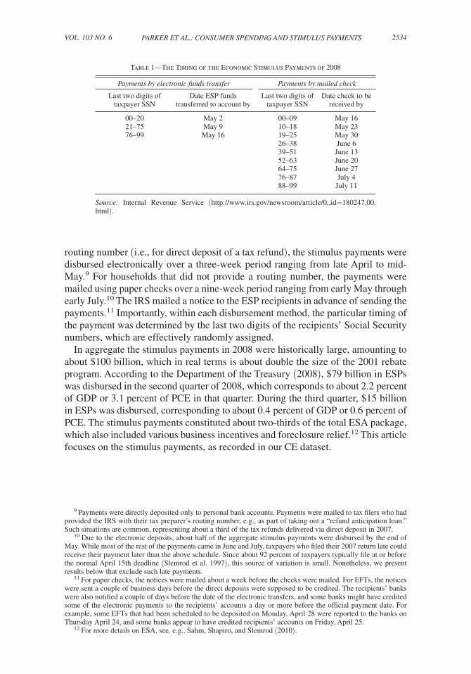
The key to our measurement strategy is that the timing of ESP disbursement was effectively randomized across households. Table 1 shows the schedule of ESP disbursement.8 For recipients that had provided the IRS with their personal bank

6 Deaton (1992), Browning and Lusardi (1996), and Jappelli and Pistaferri (2010) review the consumption-smoothing literature in general, and JPS and the working paper version of this article, Parker et al. (2011), review the tax rebate literature in particular. A complementary set of papers surveys households about how they used or plan to use their rebates (Shapiro and Slemrod (2003a, 2003b); Coronado, Lupton, and Sheiner 2006; Bureau of Labor Statistics 2009; Shapiro and Slemrod 2009; Sahm, Shapiro, and Slemrod 2010). Parker et al. (2011) analyzes the consistency of such self-reported spending with our regression-based causal estimates of the response of spend-ing. Auerbach and Gale (2010) surveys recent fiscal policy more broadly.

7 To expedite the disbursement of the payments, they were calculated using data from tax year 2007 returns (and so only those filing 2007 returns received the payments). If subsequently a household’s tax year 2008 data implied a larger payment, the household could claim the difference on its 2008 return filed in 2009. However, if the 2008 data implied a smaller payment, the household did not have to return the difference.

8 The IRS schedule reports the latest date by which the ESPs are supposed to have been received by households. Accordingly, as also discussed below, the payments were disbursed (i.e., put in the mail or electronically transferred to banks) slightly earlier.


routing number (i.e., for direct deposit of a tax refund), the stimulus payments were disbursed electronically over a three-week period ranging from late April to mid-May.9 For households that did not provide a routing number, the payments were mailed using paper checks over a nine-week period ranging from early May through early July.10 The IRS mailed a notice to the ESP recipients in advance of sending the payments.11 Importantly, within each disbursement method, the particular timing of the payment was determined by the last two digits of the recipients’ Social Security numbers, which are effectively randomly assigned.

In aggregate the stimulus payments in 2008 were historically large, amounting to about $100 billion, which in real terms is about double the size of the 2001 rebate program. According to the Department of the Treasury (2008), $79 billion in ESPs was disbursed in the second quarter of 2008, which corresponds to about 2.2 percent of GDP or 3.1 percent of PCE in that quarter. During the third quarter, $15 billion in ESPs was disbursed, corresponding to about 0.4 percent of GDP or 0.6 percent of PCE. The stimulus payments constituted about two-thirds of the total ESA package, which also included various business incentives and foreclosure relief.12 This article focuses on the stimulus payments, as recorded in our CE dataset.

9 Payments were directly deposited only to personal bank accounts. Payments were mailed to tax filers who had provided the IRS with their tax preparer’s routing number, e.g., as part of taking out a “refund anticipation loan.” Such situations are common, representing about a third of the tax refunds delivered via direct deposit in 2007.

10 Due to the electronic deposits, about half of the aggregate stimulus payments were disbursed by the end of May. While most of the rest of the payments came in June and July, taxpayers who filed their 2007 return late could receive their payment later than the above schedule. Since about 92 percent of taxpayers typically file at or before the normal April 15th deadline (Slemrod et al. 1997), this source of variation is small. Nonetheless, we present results below that exclude such late payments.

11 For paper checks, the notices were mailed about a week before the checks were mailed. For EFTs, the notices were sent a couple of business days before the direct deposits were supposed to be credited. The recipients’ banks were also notified a couple of days before the date of the electronic transfers, and some banks might have credited some of the electronic payments to the recipients’ accounts a day or more before the official payment date. For example, some EFTs that had been scheduled to be deposited on Monday, April 28 were reported to the banks on Thursday April 24, and some banks appear to have credited recipients’ accounts on Friday, April 25.

12 For more details on ESA, see, e.g., Sahm, Shapiro, and Slemrod (2010).

Table 1—The Timing of the Economic Stimulus Payments of 2008

Payments by electronic funds transfer Payments by mailed check

Last two digits of taxpayer SSN

Date ESP funds transferred to account by

Last two digits of taxpayer SSN

Date check to be received by

00–20 May 2 00–09 May 1621–75 May 9 10–18 May 2376–99 May 16 19–25 May 30

26–38 June 639–51 June 1352–63 June 2064–75 June 2776–87 July 488–99 July 11

Source: Internal Revenue Service (http://www.irs.gov/newsroom/article/0,,id=180247,00.html).


II. The Consumer Expenditure Survey

The CE interview survey contains detailed measures of the expenditures of a strat-ified random sample of US households. Households are interviewed four times, at three-month intervals, about their spending over the previous three months. Because new households are added to the survey every month, the data can be used to iden-tify spending effects from ESPs disbursed in different months.

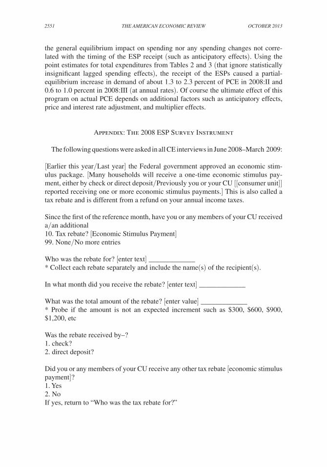
Questions about the 2008 ESPs were added to the CE survey in interviews con-ducted between June 2008 and March 2009, which covers the crucial time during which the payments were disbursed.13 The questions were phrased to be consistent with the style of other CE questions and the 2001 tax rebate questions. Households were asked whether they received any “economic stimulus payments…also called a tax rebate” since the beginning of the reference period for the interview and, if so, the amount of each payment and the date it was received. Unlike 2001, for each pay-ment households were also asked whether it was received by check or direct deposit. The Appendix contains the language of the CE survey instruments.

To maintain consistency, our use of the data follows JPS. We sum all stimulus payments received by each household in each three-month reference period to cre-ate our main economic stimulus payment variable, ESP. We use the 2007 and 2008 waves of the CE data (which include interviews in the first quarter of 2009) and analyze only households with at least one expenditure interview during the period in which the ESP questions were in the field. Finally, we focus on a series of increas-ingly aggregated measures of consumption expenditures: (i) food, which includes food consumed away from home, food consumed at home, and purchases of alco-holic beverages; (ii) strictly nondurable expenditures, which follows Lusardi (1996); (iii) nondurable expenditures, which follows previous research using the CE survey and includes semi-durable categories like apparel, health, and reading materials; (iv) total expenditures, which also includes durable expenditures such as home fur-nishings, entertainment equipment, and auto purchases.14

The responses to the CE questions match reasonably well the other limited information available about the ESPs. The average value of ESP, conditional on a positive value, is about $1,000, and about two-thirds of households reported receiv-ing rebates during the main period of their disbursement. Households that receive ESPs by EFT on average have slightly higher expenditures, are slightly younger, have higher incomes and liquid assets, and have larger ESPs than households that receive the payments by mail. Consistent with the payments specified by ESA, most reported ESPs are in multiples of $300, with about 55 percent of reports reflecting the (maximum) basic payments of $600 or $1,200. The aggregate amount of ESPs is

13 Ideally, since some ESPs arrived in April, the survey would have been in the field in May, e.g., for respondents whose last interview was in May.

14 Unlike in JPS, we find that the spending effect on total expenditures in 2008 is estimated with relative statisti-cal precision. This could in part reflect the larger number of payments (about 30 percent more) in the sample in 2008, and the larger size (over double) of these payments. Suggestive of an improvement in data quality, there is also a decline in the ratio of the standard deviation of the change in household-level expenditures to the average level of expenditures between 2001 and 2008 for all our major expenditure categories. This may be due to the CE survey’s transition in 2003 from using survey booklets to using computer-assisted personal-interview (CAPI) soft-ware. The CE survey measures expenditures independent of the use of credit or debt, so the measured expenditure for durables purchased using financing is the full price of the durable, not just the down payment.


$94.6 billion in the weighted, raw CE data, which is quite close to the $96.2 billion reported in the Daily Treasury Statements (Department of the Treasury 2008). The temporal pattern of ESP receipt is also broadly similar across the two sources, though the CE data have fewer ESPs reported during the peak month of May and more in the following months, suggesting the possibility that some households took time to notice their ESP receipt or that there is some other tendency to report a somewhat later date of receipt than actually occurred.15

III. Empirical Methodology

Consistent with specifications in the previous literature (e.g., Zeldes 1989; Lusardi 1996; Parker 1999; Souleles 1999; and JPS), our main estimating equation is

(1) C i,t+1 − C i,t = ∑ s

β 0s × month s,i + β 1 ′ X i,t + β 2 ESP i,t+1 + u i,t+1 ,

where i indexes households, and t indexes time, C is either household consumption expenditures or their log; month represents a complete set of indicator variables for every period in the sample, used to absorb the seasonal variation in consump-tion expenditures as well as the average of all other concurrent aggregate factors; and X represents control variables (age and changes in family size) included to absorb some of the preference-driven differences in the growth rate of consump-tion expenditures across households. ES P i,t+1 represents our key stimulus payment variable, which takes one of three forms: (i) the total dollar amount of payments received by household i in period t + 1 (ES P i,t+1 ); (ii) a dummy variable indi-cating whether any payment was received in t + 1 (I(ES P i,t+1 > 0)); and (iii) a distributed lag of ESP or I(ESP > 0), used to measure the longer-run effects of the payments. The key coefficient β 2 measures the average response of household expenditure to the arrival of a stimulus payment.16 To analyze heterogeneity in the response to the payments, we interact ES P i,t+1 with indicators for different types of households. We correct the standard errors to allow for arbitrary heteroskedastic-ity and within-household serial correlation.

The Euler-equation literature focuses on testing whether predictable changes in income are orthogonal to the residual ( u i,t+1 ) over time; that is, whether β 2 equals zero (Chamberlain 1984; Souleles 2004). In contrast, here we use the randomized timing of ESP receipt to ensure orthogonality between the residual and our ESP regressor in the cross-section, which allows us to estimate β 2 and, thus, measure the causal effect of the payments on expenditure, regardless of whether the LCPIH is true or not. Nonetheless, our estimate still provides a direct test of the LCPIH and Ricardian equivalence, as discussed in the introduction.17

15 Our working paper Parker et al. (2011) contains more details about the data.16 Our empirical approach estimates only the spending response correlated with the timing of the payment

receipt. Our approach cannot estimate the magnitude of any common response as may have occurred in anticipation of the payments, both because the passage of ESA cannot be separated from other aggregate effects captured by our time dummies, such as seasonality and monetary policy, and because there is no single point in time at which a tax cut went from being entirely unexpected to being entirely expected.

17 Even though February 2008, when the ESA was passed, can fall in period t for some sample households receiving a payment, under our maintained assumptions, any announcement effect does not bias our estimate of β 2 . Whenever information about the tax cuts underlying the ESPs became publicly available, whether preceding the


IV. The Short-Run Response of Expenditure

This section estimates the change in consumption expenditures caused by receipt of a stimulus payment during the three-month period of receipt, using the contem-poraneous payment variables ES P t+1 and I(ES P t+1 > 0) in equation (1). Following JPS, we begin by estimating (the average) β 2 using all available variation in the full sample and subsequently refine our identification strategy by dropping nonre-cipients and late recipients from our sample, and by using only the variation in the timing of ESP receipt within each method of disbursement (check versus EFT). The subsequent section estimates the lagged response to the payments.

A. Variation across All Households

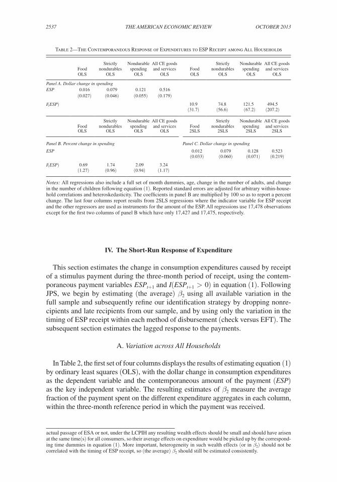
In Table 2, the first set of four columns displays the results of estimating equation (1) by ordinary least squares (OLS), with the dollar change in consumption expenditures as the dependent variable and the contemporaneous amount of the payment (ESP) as the key independent variable. The resulting estimates of β 2 measure the average fraction of the payment spent on the different expenditure aggregates in each column, within the three-month reference period in which the payment was received.

actual passage of ESA or not, under the LCPIH any resulting wealth effects should be small and should have arisen at the same time(s) for all consumers, so their average effects on expenditure would be picked up by the correspond-ing time dummies in equation (1). More important, heterogeneity in such wealth effects (or in β 2 ) should not be correlated with the timing of ESP receipt, so (the average) β 2 should still be estimated consistently.

Table 2—The Contemporaneous Response of Expenditures to ESP Receipt among All Households

FoodStrictly

nondurables Nondurable

spendingAll CE goods and services

Food

Strictly nondurables

Nondurable spending

All CE goods and services

OLS OLS OLS OLS OLS OLS OLS OLS

Panel A. Dollar change in spendingESP 0.016 0.079 0.121 0.516

(0.027) (0.046) (0.055) (0.179)

I(ESP) 10.9 74.8 121.5 494.5(31.7) (56.6) (67.2) (207.2)

FoodStrictly

nondurables Nondurable

spendingAll CE goods and services Food

Strictly nondurables

Nondurable spending


OLS OLS OLS OLS 2SLS 2SLS 2SLS 2SLS

Panel B. Percent change in spending Panel C. Dollar change in spending

ESP 0.012 0.079 0.128 0.523(0.033) (0.060) (0.071) (0.219)

I(ESP) 0.69 1.74 2.09 3.24(1.27) (0.96) (0.94) (1.17)

Notes: All regressions also include a full set of month dummies, age, change in the number of adults, and change in the number of children following equation (1). Reported standard errors are adjusted for arbitrary within-house-hold correlations and heteroskedasticity. The coefficients in panel B are multiplied by 100 so as to report a percent change. The last four columns report results from 2SLS regressions where the indicator variable for ESP receipt and the other regressors are used as instruments for the amount of the ESP. All regressions use 17,478 observations except for the first two columns of panel B which have only 17,427 and 17,475, respectively.


We find that, during the three-month period in which a payment was received, a household on average increased its expenditures on food by about 2 percent of the payment, its expenditures on strictly nondurable goods by 8 percent of the payment, and its expenditures on nondurable goods by 12 percent of the payment. The third result is statistically significant. The fourth column shows that expenditures on total consumption increased on average by 52 percent of the payment, a substantial and statistically significant amount.

These results identify the effect of a payment from variation in both the tim-ing of payment receipt and the dollar amount of the payment. While the variation in the payment amount is possibly uncorrelated with the residual in equation (1), the variation is not purely random since the payment amount depends upon house-hold characteristics such as tax status, income, and number of dependents. Unlike most previous research, we can refine the variation that we use to focus on variation known to be exogenous.

The remaining columns of Table 2 use only variation in whether any payment was received at all in a given period, not the dollar amount of payments received. The second set of columns in panel A uses the indicator variable I(ESP > 0) in equation (1). In this case β 2 measures the average dollar increase in expenditures caused by receipt of a payment. During the three-month period in which a pay-ment was received, households on average increased their nondurable expenditures by $122, which is statistically significant at the 7 percent level. Total expenditures increased by a significant $495. Compared to an average payment of just under $1,000, these results are consistent with the previous estimates in the first set of col-umns, which also used variation in the magnitude of the payments received.

As a robustness check, panel B uses the change in log expenditures as the depen-dent variable. On average in the three-month period in which a payment was received, nondurable expenditures increased by 2.1 percent, and total expenditures increased by 3.2 percent. These are statistically and economically significant effects. At the average ESP and level of nondurable and total expenditures, these results imply pro-pensities to spend of 0.120 and 0.364 respectively, which are consistent with, though slightly smaller than, the previous results in the table.

Finally, to estimate a value interpretable as a marginal propensity to spend upon payment receipt without using variation in ESP amount, we estimate equation (1) by two-stage least squares (2SLS). We instrument for the payment amount, ESP, using the indicator variable, I(ESP > 0), along with the other independent variables. As in the first set of results in panel A, β 2 then measures the fraction of the payment that is spent within the three-month period of receipt. As shown in panel C, the estimated marginal propensities to spend remain close in magnitude to those estimated in the first set of results, which did not treat ESP as potentially nonexogenous.18

18 Parker et al. (2011) discusses how these results are generally robust across a number of additional sensitivity checks. For example, using median regressions or winsorizing the dependent variable generally leads to very similar results for food and strictly nondurable goods. For nondurable goods and total expenditures, the resulting coeffi-cients are still statistically and economically significant (and substantially larger than those for strictly nondurable goods) though generally smaller than in Table 2, which is consistent with iatrogenic bias since by mostly dropping large durables purchases, one biases down the estimates of the average spending caused by the ESP.


B. Variation among Households That Receive ESPs at Some Time

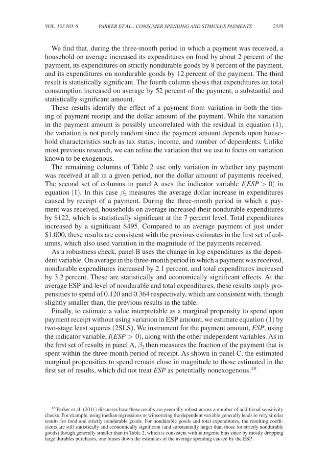
The results in panel C of Table 2 identify the effect of ESP receipt on spending by comparing the behavior of households that received payments at different times to the behavior of households that did not receive payments during those times. Since some households did not receive any payment, in any period, the results still use some information that comes from comparing households that received payments to households that never received payments. We now investigate the role of this varia-tion using a number of different approaches, for brevity focusing on nondurable expenditures and total expenditures.

First, we add to equation (1) an indicator for households that received a payment in any reference quarter, I(ES P i,t+1 > 0 for any t ) i , which allows the expenditure growth of payment recipients to differ on average from that of nonrecipients. In this case, the main regressor I(ESP > 0) captures only higher-frequency variation in the timing of payment receipt—receipt in quarter t+1 in particular—conditional on receipt in some quarter. As reported in panel A of Table 3, the estimated coefficients for the effect of the payment (ESP and I(ESP > 0)) are quite similar to those in Table 2, and the estimated coefficients on I(ES P i,t+1 > 0 for any t ) i are statistically insignificant. Hence, apart from the effect of the payment, there is little difference between the expenditure growth of payment recipients and nonrecipients over the

Table 3—The Response to ESP Receipt among Households Receiving Payments

Dollar change in Percent change in Dollar change in

Nondurable spending


Nondurable spending


Nondurable spending


OLS OLS OLS OLS 2SLS 2SLS

Panel A. Sample of all households (N = 17,478)ESP 0.117 0.507 0.123 0.509

(0.060) (0.196) (0.081) (0.253)I(ESP) 2.63 3.97

(1.07) (1.34)I(ES P i,t > 0 for any t)i 9.58 21.21 −0.88 −1.17 8.23 20.77

(36.07) (104.00) (0.50) (0.63) (38.79) (112.18)

Panel B. Sample of households receiving ESPs (N = 11,239)ESP 0.185 0.683 0.252 0.866

(0.066) (0.219) (0.103) (0.329)I(ESP) 3.91 5.63

(1.33) (1.69)

Panel C. Sample of households receiving only on-time ESPs (N = 10,488)ESP 0.214 0.590 0.308 0.911

(0.070) (0.217) (0.112) (0.342)I(ESP) 4.52 6.05

(1.50) (1.89)

Notes: All regressions also include the change in the number of adults, the change in the number of children, the age of the household, and a full set of month dummies. Reported standard errors are adjusted for arbitrary within-household correlations and heteroskedasticity. The coefficients in the second triplet of columns are mul-tiplied by 100 so as to report a percent change. The final triplet of columns report results from 2SLS regressions where the indicator variable for ESP receipt and the other regressors are used as instruments for the amount of the ESP. The variable I(ES P i,t > 0 for any t ) i is an indicator for households that received an ESP in some reference quarter, whereas I(ESP > 0) indicates receipt in the contemporaneous quarter (t+1) in particular.


quarters in the sample period around the payments, and thus such a difference is not spuriously generating the results in Table 2.

Our second approach is more stringent. We exclude from the sample all house-holds that did not report a payment in any of their interviews. The advantage of this approach is that, when we do not use variation in ESP amount, the response of spending is identified using only the variation in the timing of payment receipt conditional on receipt at some time. That is, identification comes from comparing the spending of households that received payments in a given period to the spending of households that also received payments but in other periods. The disadvantage of this approach is that it leads to a reduction in power due to the resulting decline in sample size and effective variation. Nonetheless, panel B of Table 3 shows that the estimates are broadly consistent with the previous results, although both point estimates and standard errors are somewhat larger.

Third, we drop all households that received late stimulus payments, after the main period of their (randomized) disbursement. Although the timing of late payments is not necessarily endogenous, it is not randomized. The vast majority of house-holds that received late ESPs did so due to filing late tax returns for tax year 2007, although as noted there also seem to be some lags in reporting (or in noticing) the payments in the CE survey. We follow JPS and allow one month’s “grace period” in excluding late ESPs, so that we consider a mailed payment to be late if it is reported received after August, and an electronic payment (or any payment with missing data on the method of disbursement) to be late if it is reported received after June.

Table 3 panel C shows that the results remain statistically and economically sig-nificant. In the final set of columns using 2SLS, on average nondurable expenditures increased by 31 percent of the payment in the quarter of receipt, and total expendi-tures increased by 91 percent of the payment. Given that this approach has sufficient power to identify the key parameter of interest, we focus on this sample as our main sample for the remainder of the article.

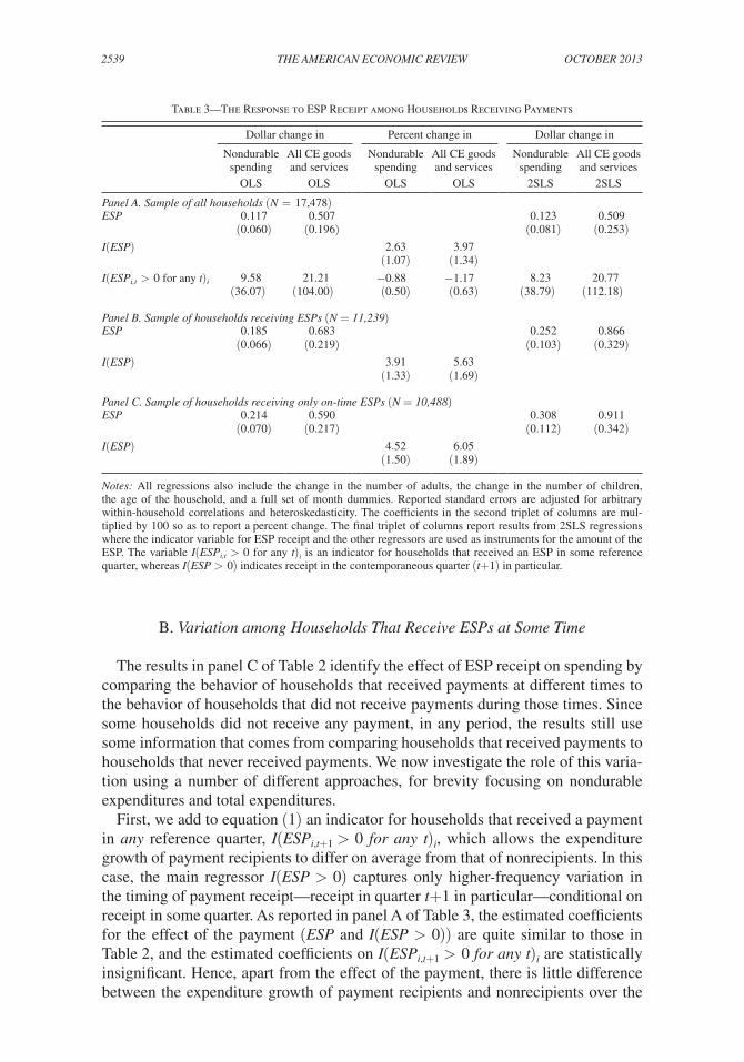
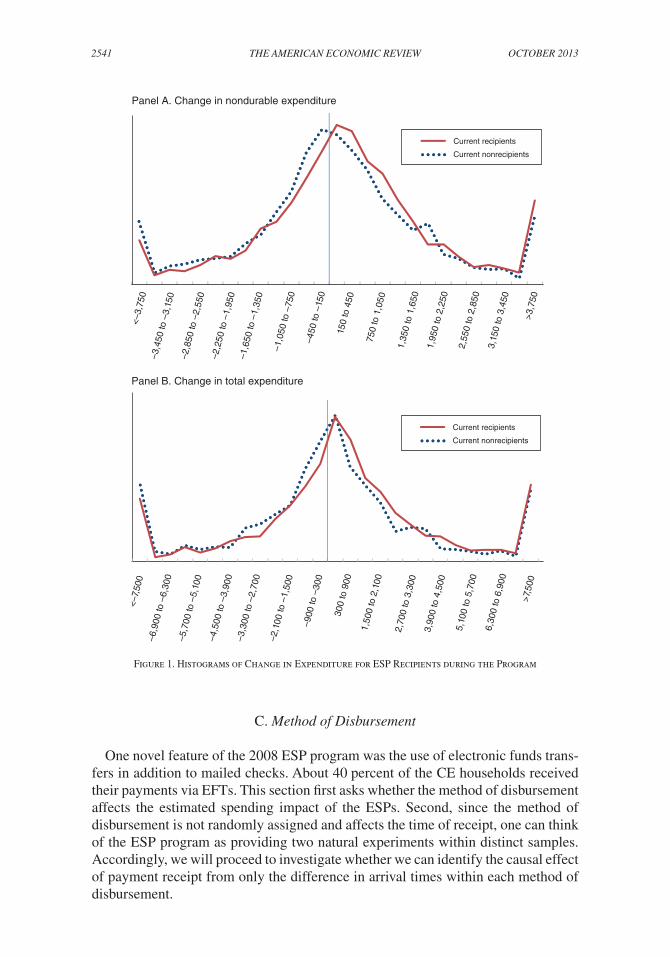
As another robustness check, Figure 1 compares the histograms of the distribution of changes in expenditure for observations during which an ESP is received versus observations during which an ESP is not received. The figure focuses on the sample of on-time recipients and the time period during which the ESPs were being dis-tributed (i.e., when the t+1 interview occurs between June 2008 and October 2008, with the corresponding expenditure reference periods covering the preceding three months). As shown, there is a larger share of recipients than nonrecipients in most ranges of increases in spending, and a larger share of nonrecipients than recipients in most ranges of decreases in spending. (Each cell in panel A represents a $300 range, and in panel B a $600 range, so these differences are economically significant). While these histograms do not control for any covariates (which affect power, not consistency), they support our main findings nonparametrically in the raw data and show that outliers are not driving the main findings. The analogous histograms are very similar for the sample in Table 2.

In sum, even when limiting the variation to the timing of ESP receipt conditional on (nonlate) receipt, the results imply that the receipt of the ESPs had a significant effect on household spending. By contrast, in JPS, analogously limiting the sample to nonlate rebate recipients leads to a larger reduction in precision and a loss of statistical significance.


C. Method of Disbursement

One novel feature of the 2008 ESP program was the use of electronic funds trans-fers in addition to mailed checks. About 40 percent of the CE households received their payments via EFTs. This section first asks whether the method of disbursement affects the estimated spending impact of the ESPs. Second, since the method of disbursement is not randomly assigned and affects the time of receipt, one can think of the ESP program as providing two natural experiments within distinct samples. Accordingly, we will proceed to investigate whether we can identify the causal effect of payment receipt from only the difference in arrival times within each method of disbursement.

Figure 1. Histograms of Change in Expenditure for ESP Recipients during the Program

Panel B. Change in total expenditure

Panel A. Change in nondurable expenditure

Current recipients

Current nonrecipients

Current recipients

Current nonrecipients

<–3,

750

–3,4

50 to

–3,

150

–2,8

50 to

–2,

550

–2,2

50 to

–1,

950

–1,6

50 to

–1,

350

–1,0

50 to

–75

0

–450

to –

150

150

to 4

50

750

to 1

,050

1,35

0 to

1,6

50

1,95

0 to

2,2

50

2,55

0 to

2,8

50

3,15

0 to

3,4

50

>3,7

50

<–7,

500

–6,9

00 to

–6,

300

–5,7

00 to

–5,

100

–4,5

00 to

–3,

900

–3,3

00 to

–2,

700

–2,1

00 to

–1,

500

–900

to –

300

300

to 9

00

1,50

0 to

2,1

00

2,70

0 to

3,3

00

3,90

0 to

4,5

00

5,10

0 to

5,7

00

6,30

0 to

6,9

00

>7,5

00


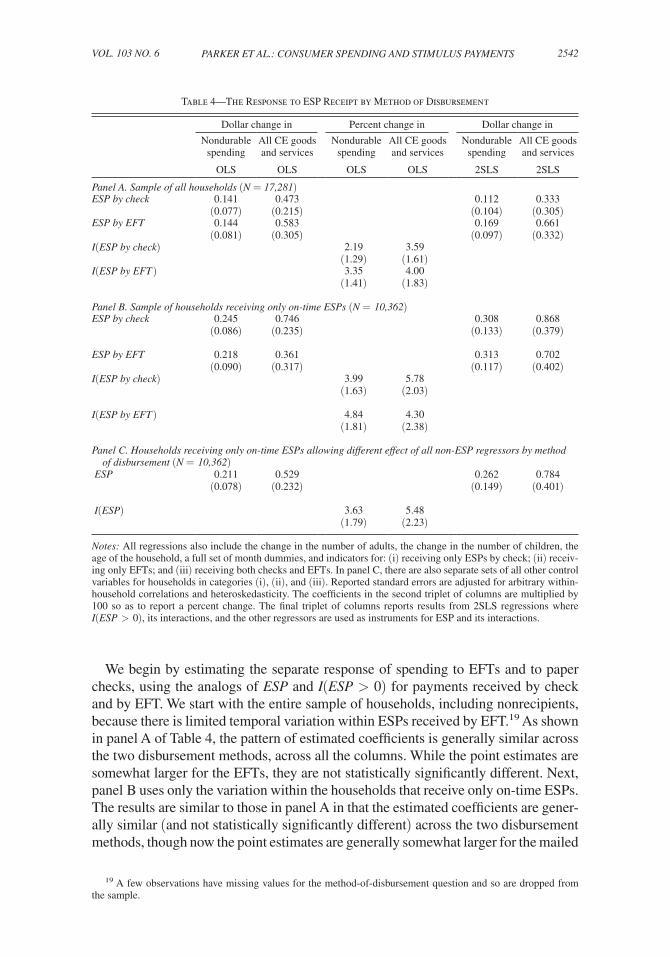
We begin by estimating the separate response of spending to EFTs and to paper checks, using the analogs of ESP and I(ESP > 0) for payments received by check and by EFT. We start with the entire sample of households, including nonrecipients, because there is limited temporal variation within ESPs received by EFT.19 As shown in panel A of Table 4, the pattern of estimated coefficients is generally similar across the two disbursement methods, across all the columns. While the point estimates are somewhat larger for the EFTs, they are not statistically significantly different. Next, panel B uses only the variation within the households that receive only on-time ESPs. The results are similar to those in panel A in that the estimated coefficients are gener-ally similar (and not statistically significantly different) across the two disbursement methods, though now the point estimates are generally somewhat larger for the mailed

19 A few observations have missing values for the method-of-disbursement question and so are dropped from the sample.

Table 4—The Response to ESP Receipt by Method of Disbursement


Nondurable spending


Nondurable spending


Nondurable spending



Panel A. Sample of all households (N = 17,281)ESP by check 0.141 0.473 0.112 0.333

(0.077) (0.215) (0.104) (0.305)ESP by EFT 0.144 0.583 0.169 0.661

(0.081) (0.305) (0.097) (0.332)I(ESP by check) 2.19 3.59

(1.29) (1.61)I(ESP by EFT ) 3.35 4.00

(1.41) (1.83)

Panel B. Sample of households receiving only on-time ESPs (N = 10,362)ESP by check 0.245 0.746 0.308 0.868

(0.086) (0.235) (0.133) (0.379)

ESP by EFT 0.218 0.361 0.313 0.702(0.090) (0.317) (0.117) (0.402)

I(ESP by check) 3.99 5.78(1.63) (2.03)

I(ESP by EFT ) 4.84 4.30(1.81) (2.38)

Panel C. Households receiving only on-time ESPs allowing different effect of all non-ESP regressors by method of disbursement (N = 10,362) ESP 0.211 0.529 0.262 0.784

(0.078) (0.232) (0.149) (0.401)

I(ESP) 3.63 5.48(1.79) (2.23)

Notes: All regressions also include the change in the number of adults, the change in the number of children, the age of the household, a full set of month dummies, and indicators for: (i) receiving only ESPs by check; (ii) receiv-ing only EFTs; and (iii) receiving both checks and EFTs. In panel C, there are also separate sets of all other control variables for households in categories (i), (ii), and (iii). Reported standard errors are adjusted for arbitrary within-household correlations and heteroskedasticity. The coefficients in the second triplet of columns are multiplied by 100 so as to report a percent change. The final triplet of columns reports results from 2SLS regressions where I(ESP > 0), its interactions, and the other regressors are used as instruments for ESP and its interactions.


checks. Not surprisingly, since the EFTs were disbursed over just a few weeks, using just timing variation leads to relatively less power for estimating the effect of EFT receipt, especially for the more volatile total expenditure category. Also, the smaller number of ESPs used to identify the effects of a mailed ESP increase standard errors as well. In sum, these results provide little evidence that the method of disbursement significantly affected the average response of spending.

We now turn to the question of whether we can identify the spending effect using only the randomized variation in spending within households that receive only on-time ESPs by check and within households that receive only on-time ESPs by EFT. This approach allows for the selection into each group to be nonrandom. For example, households receiving EFTs have somewhat higher income on average than households receiving paper checks and might also be different in other, hard-to-observe ways that could potentially be correlated with the differences in timing of the two disbursement methods.

As already discussed, panels A and B of Table 4 provide some evidence that the spending effect does not differ by method of disbursement. The coefficients in panel B in particular are identified from variation within each group. Notably, for ESPs received by mail, which provide more temporal variation, the results are sta-tistically significant and broadly similar to the average response in the final panel of Table 3. That is, even separately controlling for receipt of EFTs, using the random variation in the timing of the mailed checks still yields a significant response of spending to the mailed checks.

These results still impose common month dummies and common demographic effects (age and changes in family size) across EFT and mailed-check recipients. Also, to gauge the impact of the stimulus program, we want to estimate the average response to the stimulus payments. Accordingly, as an extension, panel C of Table 4 presents estimates from a pooled regression that allows for separate time dummies and demo-graphic effects across three groups of households: (i) households that received only paper checks; (ii) households that received only EFTs; (iii) households that received both paper checks and EFTs (only 2 percent of households). The resulting coefficient measures the average spending effect of the receipt of an ESP independent of its method of disbursement, but allowing for households to be distributed across the disbursement methods in a way that can potentially be correlated with their spending dynamics due to other factors. While slightly smaller and less statistically significant, the estimates in panel C remain broadly similar to those in panel C of Table 3, even though the former are driven only by the randomized variation in timing within each group (primarily paper checks, since the EFTs have limited timing variation).

In sum, our findings remain broadly consistent across specifications that use dif-ferent forms of variation. Of course, using different variation sometimes induces changes in the point estimates across specifications, especially for total expendi-tures, but not significantly so relative to the corresponding confidence intervals.

V. The Longer-Run Response of Expenditure

To investigate the longer-run effect of the receipt of the stimulus payments, we add the first lag of the payment variable, ES P t , as an additional regressor in equation (1). Under the maintained assumption that the differences in timing of ESP receipt are


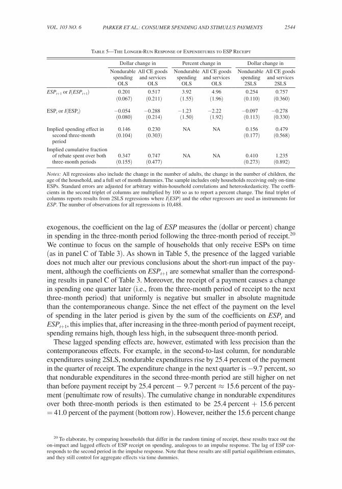
exogenous, the coefficient on the lag of ESP measures the (dollar or percent) change in spending in the three-month period following the three-month period of receipt.20 We continue to focus on the sample of households that only receive ESPs on time (as in panel C of Table 3). As shown in Table 5, the presence of the lagged variable does not much alter our previous conclusions about the short-run impact of the pay-ment, although the coefficients on ES P t+1 are somewhat smaller than the correspond-ing results in panel C of Table 3. Moreover, the receipt of a payment causes a change in spending one quarter later (i.e., from the three-month period of receipt to the next three-month period) that uniformly is negative but smaller in absolute magnitude than the contemporaneous change. Since the net effect of the payment on the level of spending in the later period is given by the sum of the coefficients on ES P t and ES P t+1 , this implies that, after increasing in the three-month period of payment receipt, spending remains high, though less high, in the subsequent three-month period.

These lagged spending effects are, however, estimated with less precision than the contemporaneous effects. For example, in the second-to-last column, for nondurable expenditures using 2SLS, nondurable expenditures rise by 25.4 percent of the payment in the quarter of receipt. The expenditure change in the next quarter is −9.7 percent, so that nondurable expenditures in the second three-month period are still higher on net than before payment receipt by 25.4 percent − 9.7 percent ≈ 15.6 percent of the pay-ment (penultimate row of results). The cumulative change in nondurable expenditures over both three-month periods is then estimated to be 25.4 percent + 15.6 percent = 41.0 percent of the payment (bottom row). However, neither the 15.6 percent change

20 To elaborate, by comparing households that differ in the random timing of receipt, these results trace out the on-impact and lagged effects of ESP receipt on spending, analogous to an impulse response. The lag of ESP cor-responds to the second period in the impulse response. Note that these results are still partial equilibrium estimates, and they still control for aggregate effects via time dummies.

Table 5—The Longer-Run Response of Expenditures to ESP Receipt


Nondurable spending


Nondurable spending


Nondurable spending



ES P t+1 or I(ES P t+1 ) 0.201 0.517 3.92 4.96 0.254 0.757 (0.067) (0.211) (1.55) (1.96) (0.110) (0.360)

ESPt or I(ESPt) −0.054 −0.288 −1.23 −2.22 −0.097 −0.278(0.080) (0.214) (1.50) (1.92) (0.113) (0.330)

Implied spending effect in 0.146 0.230 NA NA 0.156 0.479 second three-month period

(0.104) (0.303) (0.177) (0.568)

Implied cumulative fraction of rebate spent over both 0.347 0.747 NA NA 0.410 1.235 three-month periods (0.155) (0.477) (0.273) (0.892)

Notes: All regressions also include the change in the number of adults, the change in the number of children, the age of the household, and a full set of month dummies. The sample includes only households receiving only on-time ESPs. Standard errors are adjusted for arbitrary within-household correlations and heteroskedasticity. The coeffi-cients in the second triplet of columns are multiplied by 100 so as to report a percent change. The final triplet of columns reports results from 2SLS regressions where I(ESP) and the other regressors are used as instruments for ESP. The number of observations for all regressions is 10,488.


in the second period nor the 41.0 percent cumulative change is statistically significant. The second-period and cumulative changes are also insignificant for total expenditure using 2SLS. However, in the first pair of columns, using variation in the amount of the ESP increases statistical power, so that we find a statistically significant cumulative effect on spending for nondurable goods.21

In sum, we find only statistically weak evidence of an ongoing spending response. Even so, these results provide some evidence against a rapid reversal of spending, although we are unable to rule out longer-term reversals.

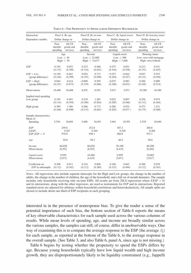
VI. Differences in Responses across Households and Goods

The leading explanation for why household spending would increase in response to a previously announced increase in income is the presence of liquidity constraints, which could make households unable or unwilling to increase spending until the receipt of an ESP.22 On the other hand, other theories propose that high-wealth or high-income households are more likely to spend their payments on receipt in part because they have smaller costs of not optimizing to fully smooth consumption over time.23

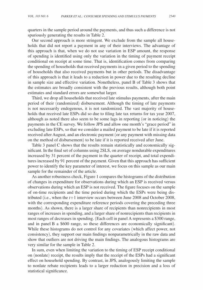
Table 6 begins by using three different proxy variables to identify households that may be disproportionately likely to be liquidity constrained (all measured as of the households’ first CE expenditure interviews): age, income (family income before taxes), and liquid assets (the sum of balances in checking and saving accounts). Following the literature, for each variable, we split households into three groups (Low and High denoting membership in the top and bottom group), with the cutoffs between groups chosen to include about a third of the payment recipients in each group. Expanding equation (1), we interact the intercept and ESP t+1 variables with Low and High for each of these proxy variables in turn. For brevity, we report only the 2SLS results.

While liquid assets is arguably the most directly relevant of the three proxy vari-ables for identifying liquidity constraints, it is the least well measured and the most often missing in the CE data. This sample selection could affect both power and con-sistency. Power is likely reduced due to the smaller samples. Consistency may or may not be affected. In whatever way the various samples in Table 6 are determined—for example on the basis of reported income, or the existence of reported income—under the assumption that the timing of ESP receipt is exogenous, the estimated β 2 coef-ficients are consistent measures of the average causal effects of interest—but only for the particular sample under consideration, not necessarily for the entire popula-tion. The estimated β 2 s and their interaction terms are what we are interested in when comparing, for instance, low-income households to high-income households: i.e., how the average treatment effect varies across income levels. But this is not what we are

21 The coefficients are generally slightly smaller and the statistical significance slightly lower in the sample comprising all households. If one adds a second lag of the ESP regressor to equation (1), the resulting estimated spending caused in the third period (relative to before receipt) is again statistically insignificant. For nondurables the point estimates are near zero. For durables, the point estimates suggest an increase in spending from the second period after receipt to the third, and as a result an even larger estimated cumulative spending effect, but these esti-mates have even greater statistical uncertainty than those reported in Table 5.

22 This constraint could reflect a hard constraint as studied in Zeldes (1989), or larger interest rates for borrowing than for saving (e.g., Davis, Kubler, and Willen 2006), or a cost for accessing illiquid wealth (e.g., Angeletos et al. 2001; Kaplan and Violante 2011).

23 See, for example, Caballero (1995); Parker (1999); Matejka and Sims (2010); and Reis (2006).


interested in in the presence of nonresponse bias. To give the reader a sense of the potential importance of such bias, the bottom section of Table 6 reports the means of key observable characteristics for each sample used across the various columns of results. While mean levels of spending, age, and income are broadly similar across the various samples, the samples can still, of course, differ in unobservable ways. One way of examining this is to compare the average response to the ESP (the average β 2 ) for each sample, as reported at the bottom of the Table 6, to the average response in the overall sample. (See Table 3, and also Table 6, panel A, since age is not missing.)

Table 6 begins by testing whether the propensity to spend the ESPs differs by age. Because young households typically have low liquid wealth and high income growth, they are disproportionately likely to be liquidity constrained (e.g., Jappelli

Table 6—The Propensity to Spend across Different Households

Interaction: Panel A. By age Panel B. By income Panel C. By liquid assets Panel D. By housing status

Dependent variable: Dollar change in Dollar change in Dollar change in Dollar change in

Non-durable

spending


Non-durable

spending


Non-durable

spending


Non-durable

spending

All CEgoods and services

Age Income Liquid assets Housing statusLow: ≤ 40 Low: ≤ 32,000 Low: ≤ 500 Low: own with mortgageHigh: > 58 High: > 74,677 High: > 7,000 High: own without

ESP 0.345 0.952 0.215 0.568 0.275 0.851 0.213 0.431 (0.133) (0.398) (0.124) (0.442) (0.164) (0.558) (0.153) (0.455)ESP × Low −0.150 −0.461 0.024 0.715 −0.253 −0.844 0.043 0.543 (group difference) (0.124) (0.399) (0.155) (0.500) (0.184) (0.527) (0.131) (0.394)ESP × High 0.044 0.414 −0.009 0.205 −0.075 0.083 0.260 0.800 (group difference) (0.151) (0.472) (0.139) (0.466) (0.186) (0.631) (0.169) (0.514)

Observations 10,488 10,488 8,592 8,592 5,071 5,071 10,380 10,380

Implied total spendingLow group 0.195 0.491 0.239 1.283 0.022 0.007 0.256 0.974

(0.114) (0.394) (0.180) (0.564) (0.205) (0.566) (0.112) (0.364)High group 0.389 1.366 0.206 0.773 0.200 0.934 0.473 1.231

(0.168) (0.498) (0.133) (0.463) (0.202) (0.677 ) (0.175) (0.508)

Sample characteristicsMean of: Spending 5,536 10,601 5,480 10,491 5,461 10,591 5,554 10,646

ESP 259.6 252.8 307.3 260.8 I(ESP) 0.267 0.264 0.320 0.268 ESP | ESP > 0 970.8 958.1 960.8 972.7

Age 50.0 50.3 48.5 50.0

Income 60,020 60,020 59,180 60,288 Observations [8,592] [8,592] [4,419] [8,494]

Liquid assets 9,959 10,480 9,959 10,002 Observations [5,071] [4,419] [5,071] [5,017]

Coefficient on 0.308 0.911 0.216 0.808 0.186 0.662 0.300 0.929 ESP in subsample (0.112) (0.342) (0.112) (0.389) (0.153) (0.494) (0.112) (0.343)

Notes: All regressions also include separate intercepts for the High and Low groups, the change in the number of adults, the change in the number of children, the age of the household, and a full set of month dummies. The sample includes only households receiving only on-time ESPs. All results are from 2SLS regressions where I(ESP > 0) and its interactions, along with the other regressors, are used as instruments for ESP and its interactions. Reported standard errors are adjusted for arbitrary within-household correlations and heteroskedasticity. All sample splits are chosen to include about one-third of ESP recipients in each grouping.


1990; Jappelli, Pischke, and Souleles 1998).24 In the first pair of columns in the table, Low refers to young households (40 years old or younger) and High refers to older households (older than 58), and the coefficients on the interaction terms with these variables represent differences relative to the households in the baseline, middle-age group. As reported, the point estimates for the interaction terms sug-gest that young households spent relatively less of the payment on receipt, and old households spent relatively more. However these differences, while economically large, are not statistically significant. Nonetheless, in absolute terms the spending by old households (see “Implied total spending” for the interacted groups) and by middle-age households (coefficient on ESP) are both statistically and economically significant, for both nondurable and total expenditure.

Panel B in Table 6 tests for differences in spending across income groups. The point estimates suggest that low-income households spent a much larger fraction of their payment upon receipt on total expenditures relative to the typical (baseline middle-income) household. However, while suggestive of a possible role for liquid-ity constraints, the difference between this result and that for the baseline group, although economically large at over 70 percent of the ESP, is not statistically signifi-cant. Nonetheless, in absolute terms for total expenditures, only the response for the low-income households is statistically significant. The response is also economically significant, averaging 128 percent of the payment.25 Note that despite losing about a quarter of the sample due to missing income data, the average sample characteristics at the bottom of panel B are similar to those for panel A (which includes the entire sam-ple, since age is not missing). Moreover, the estimated β 2 s for the sample of income reporters are also relatively close to that for the entire sample. These results do not pro-vide much reason to think that nonresponse bias is a problem in the income sample.

Panel C in Table 6 tests for differences by liquid asset holdings. While the point estimates suggest little spending by low-asset households, the associated confidence intervals are quite large, and none of the spending differences or even levels through-out the panel are statistically significant. The loss of precision when using the asset variable might reflect the smaller sample sizes due to missing asset values and mea-surement error in the available asset values. Roughly half of the data on liquid assets are missing. As noted in the final row in the table, in the resulting sample the average (uninteracted) estimated β 2 s are economically significant, but roughly a third lower in magnitude than for the entire sample of on-time recipients and also statistically insignificant. This difference is consistent with nonresponse bias in this subsample (i.e., the availability of the asset data is correlated with the treatment effect).

Relative to these results, JPS found stronger spending effects in 2001 associated with these proxies for liquidity constraints (in particular low assets). The differences with 2008 could reflect statistical uncertainty in the estimates or issues of data quality and the subsamples studied. There may also have been differences in the distribution

24 There is also evidence that older households increase their spending on receiving their (predictable) pension checks (Wilcox 1989; Stephens 2003). Outside the null LCPIH hypothesis of β2 = 0, older households might also spend relatively more because they have shorter time horizons on average.

25 It is not inconsistent for the average spending response to be larger in magnitude than the average payment, even putting aside the confidence intervals for the former, if enough households buy large durables like autos in response to receiving a payment, as found and discussed below.


of credit constraints across households between the 2001 and 2008 recessions and differences in expectations about the length and severity of the recessions.26

Another key characteristic of the recent recession was the large decline in hous-ing wealth and the reduced ability to borrow against home equity. To examine the potential implications for the response to the ESPs, we also estimate the differential spending responses across households that rented (23 percent of the sample), owned with a mortgage (50 percent), and owned without a mortgage (27 percent). The point estimates reported in panel D of Table 6 suggest that both groups of homeowners spent more of their ESPs than renters, but the differences are not statistically signifi-cant. Combining all homeowners into one group, the estimated spending responses for total expenditures are 1.051 (0.351) for homeowners and 0.434 (0.454) for renters, and these estimates are statistically significantly different at the 10 percent level.27

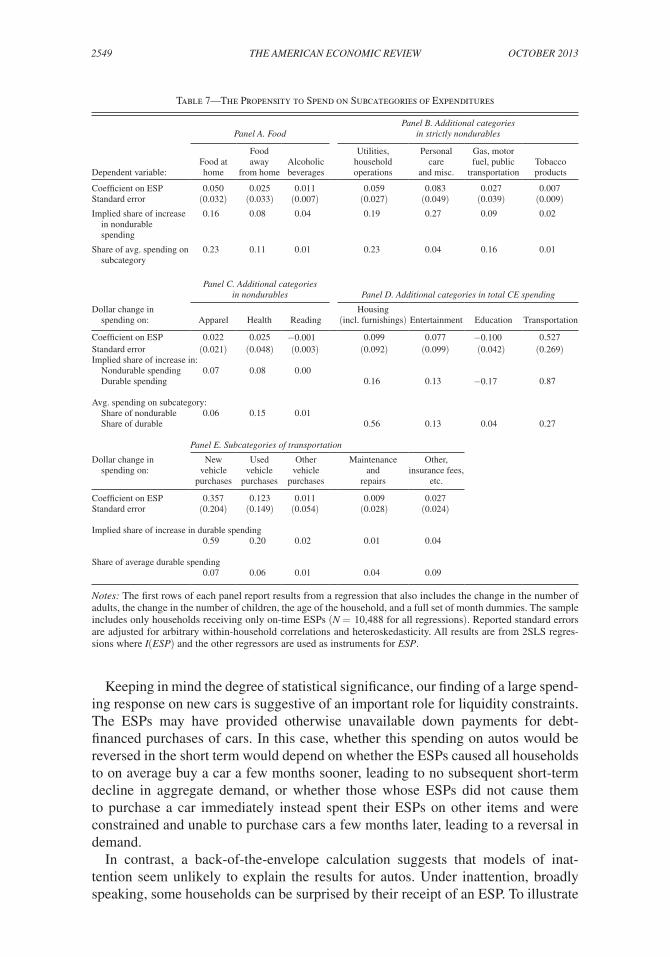
Turning to differences across types of expenditures, each column in panels A, B, and C in Table 7 reports the estimated change in spending for each subcategory of expenditures within the broad measure of nondurable expenditures (a complete decomposition). The table also reports, for each subcategory, its implied share of the total increase in nondurable spending caused by the ESP, and, for benchmarking, the average share of each subcategory in nondurable expenditures (over the entire sample). Of course, comparisons of different subsets of nondurable expenditure must be interpreted cautiously because of potential nonseparabilities across goods, and in general the greater variability in dependent variables renders the results at this level of disaggregation statistically weak. 28 Nonetheless, the point estimates suggest a disproportionately large response in alcohol, personal care (and miscel-laneous items), tobacco, and apparel.

Panel D of Table 7 provides the decomposition of the response of the durable goods and services part of total expenditures (i.e., total expenditures not in the nondurable expenditures category). The bulk of the spending response in durables (87 percent) comes in transportation, spending on which increases by 53 percent of the payments on average, a statistically and economically significant amount. This response is also large relative to the average share of transportation in durable expenditures (27 percent). Panel E in turn decomposes the response of the different subcategories of transportation. According to the point estimates, the transportation response is largely driven by purchases of vehicles, primarily new vehicles. The receipt of a stimulus payment increased the probability of purchasing a vehicle by enough to imply a large average response of total expenditures to the payments. These results imply that auto purchases, although weakening during the recession, would have been even weaker in the absence of the payments.

26 For example, if constrained households in 2008 expected the recession to last longer than usual, that would reduce the magnitude of their current response to the payment, ceteris paribus.

27 The results for homeowners do not simply reflect the preceding results for older households, e.g., if one drops from the sample the households older than 65, the resulting coefficients for nondurable expenditure remain very similar to those reported in the table, for all three groups of households in panel D. The coefficients for total expenditure remain very similar for renters and homeowners with mortgages. While the coefficient for total expen-diture loses significance for homeowners without mortgages, presumably in part due to the reduced sample of such homeowners, it remains large in magnitude; and as in the table, the coefficient for nondurable expenditure remains significant and is largest for homeowners without mortgages, compared to the other two groups.

28 Our previous results, by summing the subcategories into broader aggregates of nondurable expenditures, aver-aged out much of this unrelated variability (such as, for example, whether a trip to the supermarket happened to fall just inside or outside the expenditure reference period).


Keeping in mind the degree of statistical significance, our finding of a large spend-ing response on new cars is suggestive of an important role for liquidity constraints. The ESPs may have provided otherwise unavailable down payments for debt-financed purchases of cars. In this case, whether this spending on autos would be reversed in the short term would depend on whether the ESPs caused all households to on average buy a car a few months sooner, leading to no subsequent short-term decline in aggregate demand, or whether those whose ESPs did not cause them to purchase a car immediately instead spent their ESPs on other items and were constrained and unable to purchase cars a few months later, leading to a reversal in demand.

In contrast, a back-of-the-envelope calculation suggests that models of inat-tention seem unlikely to explain the results for autos. Under inattention, broadly speaking, some households can be surprised by their receipt of an ESP. To illustrate

Table 7—The Propensity to Spend on Subcategories of Expenditures

Panel A. FoodPanel B. Additional categories

in strictly nondurables

Dependent variable: Food athome

Foodaway

from homeAlcoholic beverages

Utilities, household operations

Personalcare

and misc.

Gas, motor fuel, public

transportationTobacco products

Coefficient on ESP 0.050 0.025 0.011 0.059 0.083 0.027 0.007Standard error (0.032) (0.033) (0.007) (0.027) (0.049) (0.039) (0.009)Implied share of increase 0.16 0.08 0.04 0.19 0.27 0.09 0.02 in nondurable spending

Share of avg. spending on 0.23 0.11 0.01 0.23 0.04 0.16 0.01 subcategory

Panel C. Additional categories in nondurables Panel D. Additional categories in total CE spending

Dollar change in spending on: Apparel Health Reading

Housing (incl. furnishings) Entertainment Education Transportation

Coefficient on ESP 0.022 0.025 −0.001 0.099 0.077 −0.100 0.527Standard error (0.021) (0.048) (0.003) (0.092) (0.099) (0.042) (0.269)Implied share of increase in: Nondurable spending 0.07 0.08 0.00 Durable spending 0.16 0.13 −0.17 0.87

Avg. spending on subcategory: Share of nondurable 0.06 0.15 0.01 Share of durable 0.56 0.13 0.04 0.27

Panel E. Subcategories of transportation

Dollar change in spending on:

Newvehicle

purchases

Used vehicle

purchases

Other vehicle

purchases

Maintenanceand

repairs

Other, insurance fees,

etc.

Coefficient on ESP 0.357 0.123 0.011 0.009 0.027Standard error (0.204) (0.149) (0.054) (0.028) (0.024)

Implied share of increase in durable spending0.59 0.20 0.02 0.01 0.04

Share of average durable spending0.07 0.06 0.01 0.04 0.09

Notes: The first rows of each panel report results from a regression that also includes the change in the number of adults, the change in the number of children, the age of the household, and a full set of month dummies. The sample includes only households receiving only on-time ESPs (N = 10,488 for all regressions). Reported standard errors are adjusted for arbitrary within-household correlations and heteroskedasticity. All results are from 2SLS regres-sions where I(ESP) and the other regressors are used as instruments for ESP.


the implications for spending, if such households spend about 10 percent of their expenditures on cars on average (over time and across households), then an increase in lifetime resources from an ESP would lead to an increase in lifetime consumption of car services of about 10 percent of the ESP. If cars were infinitely lived, then this would suggest an average increase in spending on cars of 10 percent of the ESP, a number economically (though not statistically) much lower than we find.29

VII. Conclusion

We find that on average households spent about 12 to 30 percent of their stimu-lus payments, depending on the specification, on (CE-defined) nondurable expen-ditures during the three-month period in which the payments were received. This response is larger than implied by the LCPIH or Ricardian equivalence. We also find a significant effect on the purchase of durable goods, primarily the purchase of new vehicles, bringing the average response of total consumption expenditures to about 50 to 90 percent of the payments in the quarter of receipt. These results are statisti-cally and economically significant. They remain broadly consistent and significant across specifications using different forms of variation. Indeed, the point estimates are at the high end of these ranges in specifications that focus most directly on the randomized timing of ESP receipt.

For nondurable expenditures, the estimated spending response to the 2008 ESPs is generally only slightly smaller in magnitude (and not significantly different) than the response to the 2001 tax rebates. This difference might partly reflect the more transitory nature of the 2008 tax cut. However, the composition of spending is dif-ferent than in 2001, so that the estimated spending effect on total expenditures is larger than that in 2001 due to a larger role for durables in 2008. This difference might partly reflect the larger size of the payments in 2008, or differences in macro-economic situation. (For example, the doubling in the price of oil might have made more households willing to use the rebate as a down payment to purchase a more fuel-efficient new car). That said, the overall pattern of results is generally similar in 2001 and 2008.

As in 2001, we also find some evidence of an ongoing though smaller response in the subsequent three-month period after ESP receipt, but this response cannot be estimated with precision. Regarding the implementation of the new method of delivering tax cuts, the estimated responses do not significantly differ across paper checks and electronic transfers.

Across households, according to the point estimates the spending responses are larg-est for older and low-income households, groups which have substantial and statisti-cally significant responses. By assets, the estimated spending response is largest for high-asset households, but this response is not statistically significantly different from zero, and more generally all of the asset results suffer from a lack of statistical power. Also, the estimated spending response is larger for homeowners than for renters.

Our estimates suggest a significant macroeconomic effect of the 2008 ESPs on consumer demand, although as noted in the introduction, we do not measure either

29 Since cars are finite lived, the increase in spending should be even less than 10 percent. Incorporating adjust-ment costs would further reduce the short-term response.


the general equilibrium impact on spending nor any spending changes not corre-lated with the timing of the ESP receipt (such as anticipatory effects). Using the point estimates for total expenditures from Tables 2 and 3 (that ignore statistically insignificant lagged spending effects), the receipt of the ESPs caused a partial- equilibrium increase in demand of about 1.3 to 2.3 percent of PCE in 2008:II and 0.6 to 1.0 percent in 2008:III (at annual rates). Of course the ultimate effect of this program on actual PCE depends on additional factors such as anticipatory effects, price and interest rate adjustment, and multiplier effects.

Appendix: The 2008 ESP Survey Instrument

The following questions were asked in all CE interviews in June 2008–March 2009:

[Earlier this year/Last year] the Federal government approved an economic stim-ulus package. [Many households will receive a one-time economic stimulus pay-ment, either by check or direct deposit/Previously you or your CU [[consumer unit]] reported receiving one or more economic stimulus payments.] This is also called a tax rebate and is different from a refund on your annual income taxes.

Since the first of the reference month, have you or any members of your CU received a/an additional10. Tax rebate? [Economic Stimulus Payment]99. None/No more entries

Who was the rebate for? [enter text] _____________* Collect each rebate separately and include the name(s) of the recipient(s).

In what month did you receive the rebate? [enter text] _____________

What was the total amount of the rebate? [enter value] _____________* Probe if the amount is not an expected increment such as $300, $600, $900, $1,200, etc

Was the rebate received by–?1. check?2. direct deposit?

Did you or any members of your CU receive any other tax rebate [economic stimulus payment]?1. Yes2. NoIf yes, return to “Who was the tax rebate for?”


REFERENCES

Aaronson, Daniel, Sumit Agarwal, and Eric French. 2012. “The Spending and Debt Response to Mini-mum Wage Hikes.” American Economic Review 102 (7): 3111–39.

Adams, William, Liran Einav, and Jonathan Levin. 2009. “Liquidity Constraints and Imperfect Infor-mation in Subprime Lending.” American Economic Review 99 (1): 49–84.

Agarwal, Sumit, Chunlin Liu, and Nicholas S. Souleles. 2007. “The Reaction of Consumer Spending and Debt to Tax Rebates—Evidence from Consumer Credit Data.” Journal of Political Economy 115 (6): 986–1019.

Angeletos, George-Marios, David Laibson, Andrea Repetto, Jeremy Tobacman, and Stephen Wein-berg. 2001. “The Hyperbolic Buffer Stock Model: Calibration, Simulation, and Empirical Evalua-tion.” Journal of Economic Perspectives 15 (3): 47–68.

Auerbach, Alan J., and William G. Gale. 2010. “Activist Fiscal Policy to Stabilize Economic Activity.” In Financial Stability and Macroeconomic Policy: A Symposium Sponsored by the Federal Reserve Bank of Kansas City, 327–74. Kansas City, MO: Federal Reserve Bank of Kansas City.

Barrow, Lisa, and Leslie McGranahan. 2000. “The Effects of the Earned Income Credit on the Season-ality of Household Expenditures.” National Tax Journal 53 (4): 1211–43.

Bertrand, Marianne, and Adair Morse. 2009. “What Do High-Interest Borrowers Do with Their Tax Rebate?” American Economic Review 99 (2): 418–23.

Broda, Christian, and Jonathan Parker. 2008. “The Impact of the 2008 Tax Rebates on Consumer Spending: Preliminary Evidence.” Unpublished.

Browning, Martin, and Annamaria Lusardi. 1996. “Household Saving: Micro Theories and Macro Facts.” Journal of Economic Literature 34 (4): 1797–855.

Bureau of Labor Statistics, US Department of Labor. 2009. “Consumer Expenditure Survey Results on the 2008 Economic Stimulus Payments (Tax Rebates).” http://www.bls.gov/cex/taxrebate.htm (accessed October 15, 2009).

Caballero, Ricardo J. 1995. “Near-Rationality, Heterogeneity, and Aggregate Consumption.” Journal of Money, Credit, and Banking 27 (1): 29–48.

Chamberlain, Gary. 1984. “Panel Data.” In Handbook of Econometrics. Vol. 2, edited by Zvi Griliches and Michael D. Intriligator, 1247–1318. Amsterdam: Elsevier, North-Holland.

Coronado, Julia Lynn, Joseph P. Lupton, and Louise M. Sheiner. 2006. “The Household Spending Response to the 2003 Tax Cut: Evidence from Survey Data.” Board of Governors of the Federal Reserve System (US), Finance and Economics Discussion Series: 2005–32.

Davis, Steven J., Felix Kubler, and Paul Willen. 2006. “Borrowing Costs and the Demand for Equity over the Life Cycle.” Review of Economics and Statistics 88 (2): 348–62.

Deaton, Angus. 1992. Understanding Consumption. New York: Oxford University Press.Jappelli, Tullio. 1990. “Who Is Credit Constrained in the US Economy?” Quarterly Journal of Eco-

nomics 105 (1): 219–34.Jappelli, Tullio, Jörn-Steffen Pischke, and Nicholas S. Souleles. 1998. “Testing for Liquidity Con-

straints in Euler Equations with Complementary Data Sources.” Review of Economics and Statistics 80 (2): 251–62.

Jappelli, Tullio, and Luigi Pistaferri. 2010. “The Consumption Response to Income Changes.” Annual Review of Economics 2 (1): 479–506.

Johnson, David S., Jonathan A. Parker, and Nicholas S. Souleles. 2006. “Household Expenditure and the Income Tax Rebates of 2001.” American Economic Review 96 (5): 1589–610.

Johnson, David S., Jonathan A. Parker, and Nicholas S. Souleles. 2009. “The Response of Consumer Spending to Rebates During an Expansion: Evidence from the 2003 Child Tax Credit.” Unpublished.

Kaplan, Greg, and Giovanni L. Violante. 2011. “A Model of the Consumption Response to Fiscal Stimulus Payments.” National Bureau of Economic Research Working Paper 17338.

Leininger, Lindsey, Helen Levy, and Diane Schanzenbach. 2010. “Consequences of SCHIP Expan-sions for Household Well-Being.” Forum for Health Economics and Policy 13 (1): 1–32.

Lusardi, Annamaria. 1996. “Permanent Income, Current Income, and Consumption: Evidence from Two Panel Datasets.” Journal of Business and Economic Statistics 14 (1): 81–90.

Matejka, Filip, and Christopher A. Sims. 2010. “Discrete Actions in Information-Constrained Track-ing Problems.” Unpublished.

Mian, Atif, and Amir Sufi. 2012. “The Effects of Fiscal Stimulus: Evidence from the 2009 Cash for Clunkers Program.” Quarterly Journal of Economics 127 (3): 1107–42.

Misra, Kanishka, and Paolo Surico. 2011. “Heterogeneous Responses and Aggregate Impact of the 2001 Income Tax Rebates.” Centre for Economic Policy Research Discussion Paper 8306.

http://pubs.aeaweb.org/action/showLinks?system=10.1257%2Faer.102.7.3111


http://pubs.aeaweb.org/action/showLinks?crossref=10.2307%2F1392101





http://pubs.aeaweb.org/action/showLinks?crossref=10.1093%2Fqje%2Fqjs024


http://pubs.aeaweb.org/action/showLinks?crossref=10.1162%2Frest.88.2.348

http://pubs.aeaweb.org/action/showLinks?crossref=10.1146%2Fannurev.economics.050708.142933

http://pubs.aeaweb.org/action/showLinks?system=10.1257%2Fjep.15.3.47



Parker, Jonathan A. 1999. “The Reaction of Household Consumption to Predictable Changes in Social Security Taxes.” American Economic Review 89 (4): 959–73.

Parker, Jonathan A., Nicholas S. Souleles, David S. Johnson, and Robert McClelland. 2011. “Con-sumer Spending and the Economic Stimulus Payments of 2008.” National Bureau of Economic Research Working Paper 16684.

Parker, Jonathan A., Nicholas S. Souleles, David S. Johnson, and Robert McClelland. 2013. “Con-sumer Spending and the Economic Stimulus Payments of 2008: Dataset.” American Economic Review. http://dx.doi.org/10.1257/aer.103.6.2530.

Reis, Ricardo. 2006. “Inattentive Consumers.” Journal of Monetary Economics 53 (8): 1761–800.Sahm, Claudia R., Matthew D. Shapiro, and Joel Slemrod. 2010. “Household Response to the 2008

Tax Rebates: Survey Evidence and Aggregate Implications.” In Tax Policy and The Economy. Vol. 24, edited by Jeffrey R. Brown, 69–110. Chicago: University of Chicago Press.

Shapiro, Matthew D., and Joel Slemrod. 2003a. “Consumer Response to Tax Rebates.” American Eco-nomic Review 93 (1): 381–96.

Shapiro, Matthew D., and Joel Slemrod. 2003b. “Did the 2001 Tax Rebate Stimulate Spending? Evi-dence from Taxpayer Surveys.” In Tax Policy and the Economy. Vol. 17, edited by James Poterba, 83–110. Cambridge, MA: MIT Press.

Shapiro, Matthew D., and Joel Slemrod. 2009. “Did the 2008 Tax Rebates Stimulate Spending?” American Economic Review 99 (2): 374–79.

Slemrod, Joel, Charles Christian, Rebecca London, and Jonathan A. Parker. 1997. “April 15 Syn-drome.” Economic Inquiry 35 (4): 695–709.

Souleles, Nicholas S. 1999. “The Response of Household Consumption to Income Tax Refunds.” Amer-ican Economic Review 89 (4): 947–58.

Souleles, Nicholas S. 2004. “Expectations, Heterogeneous Forecast Errors, and Consumption: Micro Evidence from the Michigan Consumer Sentiment Surveys.” Journal of Money, Credit, and Bank-ing 36 (1): 39–72.

Stephens, Melvin, Jr. 2003. ““3rd of tha Month”: Do Social Security Recipients Smooth Consumption between Checks?” American Economic Review 93 (1): 406–22.

US Department of the Treasury, Financial Management Service. 2008. “Daily Treasury Statement.” Various Issues. Washington, DC: Government Printing Office.

Wilcox, David W. 1989. “Social Security Benefits, Consumption Expenditure, and the Life Cycle Hypothesis.” Journal of Political Economy 97 (2): 288–304.

Zeldes, Stephen P. 1989. “Consumption and Liquidity Constraints: An Empirical Investigation.” Jour-nal of Political Economy 97 (2): 305–46.

http://pubs.aeaweb.org/action/showLinks?crossref=10.1016%2Fj.jmoneco.2006.03.001


http://pubs.aeaweb.org/action/showLinks?system=10.1257%2F000282803321455386


http://pubs.aeaweb.org/action/showLinks?crossref=10.1111%2Fj.1465-7295.1997.tb01958.x

http://pubs.aeaweb.org/action/showLinks?system=10.1257%2F000282803321455368



http://pubs.aeaweb.org/action/showLinks?system-d=10.1257%2Faer.103.6.2530

http://pubs.aeaweb.org/action/showLinks?crossref=10.1353%2Fmcb.2004.0007


“consumer spending and the economic stimulus payments of

Documents