consumption and house prices in the great recession · consumption and house prices in the great...
TRANSCRIPT

Consumption and House Prices in the Great Recession∗
Greg Kaplan†, Kurt Mitman‡, and Giovanni L. Violante§
October 25, 2016
PRELIMINARY AND INCOMPLETEPLEASE DO NOT CIRCULATE WITHOUT PERMISSION
Abstract
We build a heterogeneous-agent life-cycle incomplete-markets model of the US economywith multiple aggregate shocks (income, financial deregulation, and beliefs) leading to fluc-tuations in equilibrium house prices. Through a series of counterfactual numerical experi-ments, we address three questions. First, what was the main source of the boom and bustin house prices? We find that the belief shock plays a chief role in the behavior of pricesand rents. Financial deregulation alone was unimportant, but its interaction with the othershocks explains the dynamics of home-ownership, leverage, and cash-out refinancing. Themodel’s cross-sectional implications are in line with the ‘new narrative’ of the crisis that em-phasizes the role of middle- and high-income households. Second, how much of the dynam-ics of US nondurable consumption around the Great Recession was caused by the boom-bustof house prices? Our model suggests that changes in house prices alone can explain at least1/2 of the corresponding boom-bust in expenditures, mostly occurring through a wealth ef-fect rather than tightening access to credit. Third, would a massive debt forgiveness policyhave cushioned the macroeconomic bust and accelerated the recovery? Our simulations im-ply that such government intervention would have dramatically reduced foreclosure rates,but would have had a trivial impact on the collapse of house prices and consumption expen-ditures. Finally, our model illustrates how the size of the elasticity of consumption to houseprices depends crucially on the underlying shock that moves house prices. This finding hasconsequences for the use of sufficient-statistic approaches in this context.
Keywords: Beliefs, Consumption, Financial Deregulation, Great Recession, House Prices.
JEL Classification: E21, E30, E40, E51.
∗We thank numerous seminar participants for useful comments, and we are grateful to our discussants JoaoCocco, Ralph Luetticke, Jochen Mankart and Pietro Riechlin.
†University of Chicago, IFS and NBER‡Institute for International Economic Studies, Stockholm University and CEPR§New York University, CEPR, IFS and NBER.
1 Introduction
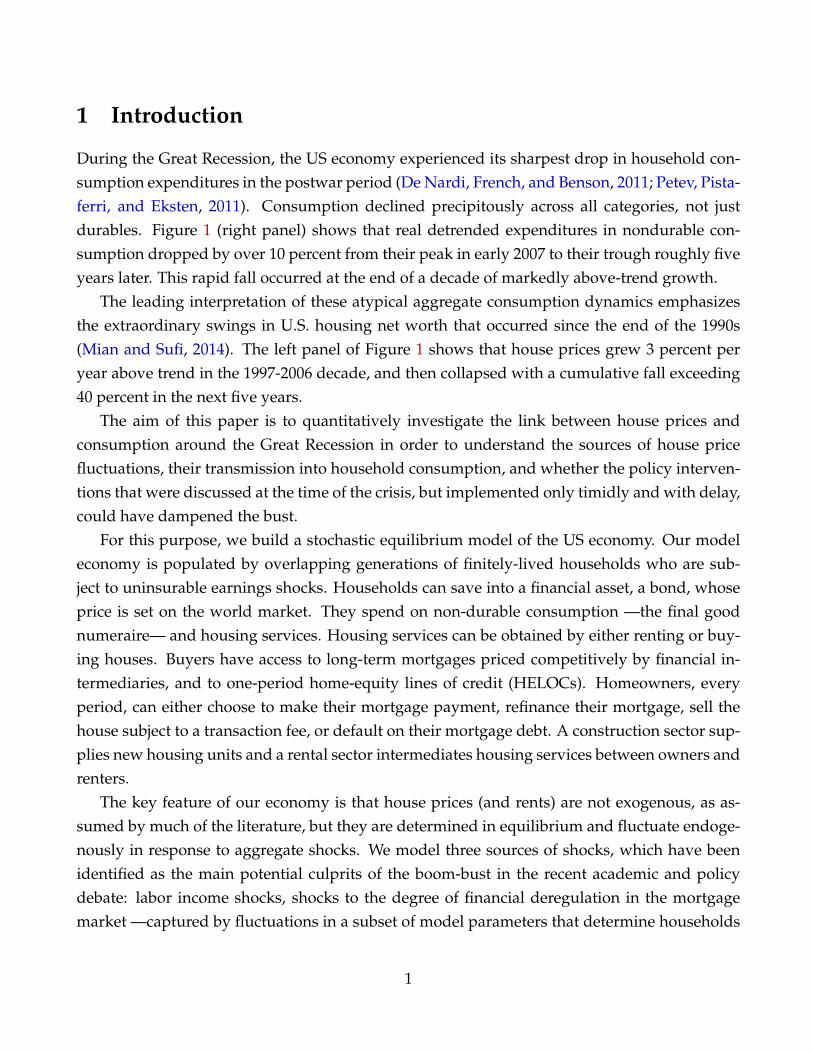
During the Great Recession, the US economy experienced its sharpest drop in household con-sumption expenditures in the postwar period (De Nardi, French, and Benson, 2011; Petev, Pista-ferri, and Eksten, 2011). Consumption declined precipitously across all categories, not justdurables. Figure 1 (right panel) shows that real detrended expenditures in nondurable con-sumption dropped by over 10 percent from their peak in early 2007 to their trough roughly fiveyears later. This rapid fall occurred at the end of a decade of markedly above-trend growth.
The leading interpretation of these atypical aggregate consumption dynamics emphasizesthe extraordinary swings in U.S. housing net worth that occurred since the end of the 1990s(Mian and Sufi, 2014). The left panel of Figure 1 shows that house prices grew 3 percent peryear above trend in the 1997-2006 decade, and then collapsed with a cumulative fall exceeding40 percent in the next five years.
The aim of this paper is to quantitatively investigate the link between house prices andconsumption around the Great Recession in order to understand the sources of house pricefluctuations, their transmission into household consumption, and whether the policy interven-tions that were discussed at the time of the crisis, but implemented only timidly and with delay,could have dampened the bust.
For this purpose, we build a stochastic equilibrium model of the US economy. Our modeleconomy is populated by overlapping generations of finitely-lived households who are sub-ject to uninsurable earnings shocks. Households can save into a financial asset, a bond, whoseprice is set on the world market. They spend on non-durable consumption —the final goodnumeraire— and housing services. Housing services can be obtained by either renting or buy-ing houses. Buyers have access to long-term mortgages priced competitively by financial in-termediaries, and to one-period home-equity lines of credit (HELOCs). Homeowners, everyperiod, can either choose to make their mortgage payment, refinance their mortgage, sell thehouse subject to a transaction fee, or default on their mortgage debt. A construction sector sup-plies new housing units and a rental sector intermediates housing services between owners andrenters.
The key feature of our economy is that house prices (and rents) are not exogenous, as as-sumed by much of the literature, but they are determined in equilibrium and fluctuate endoge-nously in response to aggregate shocks. We model three sources of shocks, which have beenidentified as the main potential culprits of the boom-bust in the recent academic and policydebate: labor income shocks, shocks to the degree of financial deregulation in the mortgagemarket —captured by fluctuations in a subset of model parameters that determine households
1
1974 1979 1984 1989 1994 1999 2004 2009 2014−0.1
−0.08
−0.06
−0.04
−0.02
0
0.02
0.04
0.06
0.08
0.1
Year
Logs
(19
97:Q
1=0)
Real ND Consumption
1974 1979 1984 1989 1994 1999 2004 2009 2014
−0.2
−0.1
0
0.1
0.2
0.3
Year
Logs
(19
97:Q
1=0)
Real House Prices
Boom
BustBust
Boom
Figure 1: Left panel: FHFA national house price index deflated by the price index of expendituresin nondurable and services. Right panel: Real consumption expenditures in nondurables and services(BEA, NIPA Table 1.1.5). Both series are deviations from linear time trends estimated separately over theperiod 1975-1996. The Boom is defined as the decade 1997-2007 and the bust as the post-2007 period.
borrowing limits and borrowing costs— and changing beliefs about future house price growth.This latter shock is modeled as a shift between two regimes that differ in the likelihood of a tran-sition into a third regime where all households have stronger preference for housing, relativeto nondurable consumption: this modeling expedient has a ‘bubble-like’ flavor, but it allowsus to maintain a rational-expectation solution of the dynamic equilibrium. To discipline thecalibration of this last stochastic process, we use survey data on expectations of future houseappreciation during the early 2000s.
The model is parameterized to match life-cycle and cross-sectional patterns of income, con-sumption, assets and liabilities of US households in the period preceding the boom and bust(end of the 1990s). The boom-bust episode is modeled as a particular realization of our ag-gregate shocks where: (i) labor income rises and then falls back; (ii) financial constraints inmortgage markets loosen (in the boom) and then tighten again (in the bust); and (iii) a switchtakes place from a regime where the transition towards a high taste for housing state is unlikelyinto a regime where such transition is likely (boom) and back (bust). We study IRF’s of the ag-gregate economy to these shocks and run a series of counterfactual experiments to answer threequestions that have been at the core of the academic and public policy debate on the housingcrisis.
First, which one of these shocks was responsible for the boom-bust in house prices aroundthe Great Recession? Our model suggests unequivocally that the change in beliefs was the
2
driving force of house price dynamics. Financial deregulation alone plays only a minor part inaccounting for the observed evolution of house prices, but its interaction with beliefs is impor-tant in explaining homeownership, leverage, and refinancing behavior. As we explain in thepaper, the limited role of loosening and tightening of loan-to-value ratio limits finds an expla-nation in the existence of rental markets and the fact that mortgages are long-term contracts,two realities that are omitted in most of the literature.
We also show that, because expectations of house appreciation are shared by all borrow-ers —rich and poor, low-risk and high-risk— the model predicts that mortgage credit growthoccurs uniformly across the household distribution. This implication is consistent with a newnarrative of the crisis that has recently emerged thanks to more detailed micro data (Adelino,Schoar, and Severino, 2016; Albanesi, De Giorgi, Nosal, and Ploenzke, 2016; Foote, Loewenstein,and Willen, 2016).
Second, how much, and through which mechanism, did household consumption fall be-cause of the collapse in house prices? Our model suggests that at a minimum half of the boom-bust in consumption over the 1997-2011 period is attributable to house price dynamics —moreif one takes the view that a portion of the decline in labor income was caused by the collapse inhousing net worth. Our model attributes only a small role to forced deleveraging and collateraleffects and implies that aggregate consumption dropped because of a wealth effect.
Third, during the housing crisis, a number of policymakers and commentators advocatedthe implementation of a massive government-sponsored debt relief programs as a way to cush-ion the collapse of house prices and expenditures. The policies of the Obama administrationconsisted of interventions (e.g., HAMP and HARP) that, because of their complex rules and nar-row scope, had very limited success (Agarwal, Amromin, Ben-David, Chomsisengphet, Pisko-rski, and Seru, 2012). We use the model to run a counterfactual where, at the onset of the bust,the government unexpectedly announces a principal reduction program whereby all mortgagedebt in excess of 95 percent of home values is cancelled, with the government repaying thelender. In the model, this policy helps roughly 1/4 of homeowners. In spite of its large scale,we show that the policy would only have a trivial effect on house prices and consumption,despite significantly lessening aggregate leverage and, as a consequence, foreclosure rates.
Finally, our structural equilibrium model sheds new light on the ‘common factor’ problemthat plagues the empirical literature that attempts to estimate, at the micro and macro level, theelasticity of consumption expenditures to house prices.1 We argue that the search for ‘the’ rightvalue of this elasticity is vacuous because the elasticity itself varies dramatically depending
1See, for example, Campbell and Cocco (2007), Carroll, Otsuka, and Slacalek (2011), Browning, Gørtz, andLeth-Petersen (2013), Mian and Sufi (2014), Mian, Rao, and Sufi (2013)
3

on which underlying shock generates the movement in house prices: changes in house pricesinduced by aggregate income shocks have the highest elasticity, whereas those caused by relax-ations or tightening of collateral constraints have the lowest impact on consumption (possiblynegative). Expenditure elasticities to house prices movements brought about by belief andinterest rate shocks are in between. We emphasize that, rather than looking for ‘exogenous’sources of variation in house prices to estimate an elasticity that has no clear and interestingempirical counterpart, it is more productive to grasp the reality that different, historically rel-evant, macroeconomic shocks transmit to household consumption, through house prices, withdifferent intensity.
This result has implications for the use of the sufficient statistic approach (as advocated,for example, in Chetty (2008)) to this question. In a recent paper, Berger, Guerrieri, Lorenzoni,and Vavra (2015) propose a clever and easy to compute ’sufficient statistic’ to estimate the indi-vidual (micro) elasticity of consumption to house prices. We show that their sufficient statisticprovides a good approximation to the true value (through the eyes of our model) in the con-text of the Great Recession. The reason is that the belief shock, which drives equilibrium pricedynamics in this boom-bust episode, is largely orthogonal to other determinants of consump-tion decisions, and thus it is akin to house price shocks in housing demand models where suchprices are exogenous, as in Berger et al. (2015). At the same time we caution against the useof this approach by showing that when house prices dynamics are caused by other shocks thesufficient statistic fails, sometimes quite dramatically, in mimicking the true elasticity.
1.1 Related Literature
[To Be Completed]
The rest of the paper is organized as follows. Section 2 outlines the model, the equilibriumconcept, and our approach to numerical computation. Section 3 describes the model’s parame-terization and its empirical fit. Section 4 presents the results from all our numerical experimentson the boom-bust. Section 5 discusses the shock- and state-dependence of the elasticity of ag-gregate consumption to house prices, and the implications for the sufficient statistic approachto this question. Section 6 concludes the paper. The Appendix [TBC] includes more detailsabout the computational algorithm, including some accuracy tests.
4
2 Model
It is useful to succinctly delineate the main features of the model, before providing a formaldescription. The economy is populated by overlapping generations of households whose life-cycle is divided between work and retirement. During the working stage, they are subject touninsurable idiosyncratic shocks to their efficiency units of labor, supplied inelastically. House-hold can save into a financial asset, a bond, whose price is set on the world market. Theyconsume non-durable consumption —the final good numeraire— and housing services. Hous-ing services can be obtained by either renting or buying houses that come in a finite number ofsizes. The rental stock is owned by a competitive rental sector. Buyers have access to long-termmortgages priced competitively by financial intermediaries. Homeowners who do not sell caneither choose to make their mortgage payment, refinance or default on their mortgage. Default-ing results in foreclosure by the intermediary which entails a utility loss, and an exacerbateddepreciation for the house. Owning a house allows the homeowner to open HELOCs, modeledas one-period non-defaultable debt-contracts. A competitive construction sector supplies newhousing units every period.
Three types of exogenous aggregate shocks can impact the economy every period: interestrates, the degree of financial regulation in the mortgage market, and beliefs about future tastefor housing. It is convenient to postpone the exact definition of these shocks to Section 2.5, afterwe have outlined the rest of the model in detail.
In illustrating the model, we begin with all the model primitives that are needed to describehousehold decisions, and we lay out the household problems. Next, we present the financialintermediation sector, the rental side, and the production side of the economy. Finally, we definethe equilibrium. Throughout, we adopt a recursive formulation of the economic environmentin discrete time.
2.1 Households
Demographics: The economy is populated by a measure-one continuum of finitely-lived house-holds. Age is indexed by j = 1, 2, · · · , J. Households work in the first phase of their life cycleand, at age Jret, they retire. They all die with certainty at age J.
Preferences: Expected lifetime utility of the household is given by:
E0
[J
∑j=1
βj−1uj(cj, sj) + βJv()
](1)
5
where β > 0 is the discount factor, cj > 0 is consumption of non-durables at age j, sj > 0is the consumption of housing services. Nondurable consumption is the numeraire good ofthe economy. The expectation is taken over sequences of aggregate and idiosyncratic shocksthat we specify below. The function v measures the felicity from leaving bequests > 0.2
Specifically, for u we assume:
uj(cj, sj
)=
ej
[(1 − ϕ) c1−γ
j + ϕs1−γj
] 1−ϑ1−γ − 1
1 − ϑ, (2)
where ϕ measures the relative taste for housing, 1/γ measures the elasticity of substitution be-tween housing services and non-durables, and 1/ϑ measures the IES. The expenditures equiva-lence scale
ej
captures deterministic changes in household size and composition over the lifecycle and explains why the intra-period utility function u is indexed by j.
The warm-glow bequest motive at age J takes the functional form:
v () = ψ(+ )1−ϑ − 1
1 − ϑ, (3)
as proposed by De Nardi et al. (2011): the term ψ measures the strength of the bequest motive,while reflects the extent to which bequests are luxury goods.
Endowments: Working households receive an idiosyncratic labor income endowment ywj given
by:log yw
j = Z + χj + ϵj (4)
where Z is an index of aggregate labor productivity. Individual labor productivity has twoorthogonal components: χj is a deterministic age profile, and ϵj follows an idiosyncratic first-order Markov process. Households are born with initial wealth endowment b1 drawn froman exogenous distribution that integrates up to the overall amount of wealth bequeathed inthe economy by the deceased households. The draw is correlated with the initial draw of ϵ1.We also denote by Υj the age-dependent transition matrix for earnings and by Υ∗
j the earningsdistribution at age j.
Housing: In order to consume housing services, households have the option of renting orowning a home. Houses are characterized by their size, whose number is finite. For owner-
2This bequest motive prevents households from selling their house and dis-saving too much during retirement,which would be counterfactual.
6

occupied housing, house size belongs to the set H = h0, ..., hN, where h0 < h1, ..., hN−1 < hN.For rental units, size belongs to the set H = h0, ..., hN.
Renting generates housing services one-for-one with the size of the house, i.e. sj = hj.To capture the fact there may be additional utility from home ownership, we assume that anowner-occupied house generates sj = ωhj units of housing services, with ω > 1. The rentalrate of a unit of housing is denoted by ρ. The per-unit price of housing is denoted by ph.Owner-occupied houses carry a per-period maintenance and tax cost of (δh + τh)phh, expressedin units of the numeraire good. Maintenance fully offsets physical depreciation of the dwellingδh. When a household sells its home, it incurs a transaction cost κh(phh), linear in the housevalue.
Financial Instruments: Households can save in one-period bonds, b, at the price qb exoge-nously determined by the net supply of financial assets from the rest of the world. It is conve-nient to also define the interest rate on bonds rb := 1/qb − 1. We allow homeowners to accessHELOCs: they can borrow up to a fraction λb of the value of their house at an interest equal tor−b = rb (1 + ιb) , where ιb > 0 is an intermediation wedge.3
Housing purchases can be financed by taking on mortgages. All mortgages are long-termand amortized over the remaining life of the buyer at the real interest rate rm equal to rb timesthe wedge (1 + ιm), with ιm > 1. Newly originated mortgages are subject to a fixed originationcost κm. They must also respect a maximum loan-to-value (LTV) ratio limit: the initial principalbalance m must be less than a fraction λm of the value of the home. Note that, once a mortgageis originated, there is no further requirement that m < λm phh. This realistic assumption, crucialto understanding deleveraging behavior and, thus, the consumption response to house priceshocks, sets our model apart from several notable contributions in this literature (Favilukis,Ludvigson, and Van Nieuwerburgh, 2010; Iacoviello and Neri, 2010)).
A household of age j that takes out a mortgage with principal balance m receives qmm unitsof the numeraire good in the current period, with qm ≤ 1. Thus, the down payment requiredby the household at origination is phh − qmm. Note that the principal due on a mortgage ofsize m is not equal to the funds received from the bank at the time of purchase (qmm) becausethe pricing of the mortgage accounts for the possibility of default, a choice that depends onall individual and aggregate states.4 Section 2.2 below provides the exact expression for theequilibrium price qm.
3In what follows to lighten the exposition, with a slight abuse of notation, we keep denoting the interest rateon liquid assets rb but it is implicit that it equals r−b when b < 0. We use a similar convention for qb.
4One can interpret this gap as so-called “points” or other up-front interest rate charges that households facewhen taking out their loans.
7

Going forward, the household makes J − j equal mortgage payments πm that must exceedthe minimum mortgage payment:
π∗ (m) =rm(1 + rm)J−j
(1 + rm)(J−j) − 1m, (5)
and the remaining principal evolves as m′ = m(1 + rm)− π. Even though all households paythe same interest rate rm on the principal due, the heterogeneity in principals m and prices qm
maps into heterogeneous effective interest rates. In simulations, when a household originatesa mortgage of size m, we can use qm and π∗ (m) to solve for the effective interest rate r∗m on themortgage through the relationship:
π∗ (m)
qmm=
r∗m(1 + r∗m)J−j
(1 + r∗m)(J−j) − 1. (6)
This formula solves for the interest rate r∗m that would yield constant mortgage payment sched-ule π∗ (m) on an outstanding balance of qmm (the funds received at origination).5
Mortgage holders have the option to refinance, by repaying the residual principal balanceand originating a new mortgage at cost κm. If a household chooses to sell its home, it is alsorequired to pay off its remaining mortgage balance. Households also have the option to defaulton their mortgage debt. Upon default, mortgages are designated as the primary lien on thehouse, implying that the proceeds from the foreclosure are disbursed to the mortgagee. We as-sume no recourse in case of foreclosure. Foreclosing reduces the value of the house to the lenderbecause it is the lender who must pay property taxes τh and maintenance, and the foreclosedhouse depreciates at a higher rate than regular houses, i.e. depreciation in case of foreclosureis δd
h > δh. Thus the lender recovers min(
1 − δdh − τh
)phh, (1 + rm)m
. A household who
defaults incurs a utility penalty ξ in the period of default.
Government: The government spends an amount G on services that are not valued by house-holds. It also runs a PAYG social security system. Retirees receive social security benefitsyret(ϵJw), where the argument of the benefit function proxies for average gross lifetime earn-ings. In what follows, we adopt the notation yj for income at age j, with the convention that ifj < Jret then yj = yw
j and yj = yret otherwise. We also denote by Υ∗ret the income distribution for
retirees.5A richer model would allow the households to simultaneously choose the amortization interest rate rm and
the principal m so that effectively they could choose qmm, as is common in the data. However, this formulationwould add a state variable (the amortization rate). For tractability we impose the fixed amortization interest rates.
8
To finance these expenditures, the government levies a property tax τh on the value of thehouse, a flat payroll tax τss and a progressive labor income tax τy(yj). Households can deductthe interest paid on mortgages against their taxable income. We denote the combined incometax liability function T (yj, mj). A final source of revenues for the government comes from theproceedings of the sale of new land permits for construction, as described in more detail inSection 2.3 below.
2.1.1 Household Decision Problems
To simplify the notation, we let Ω ∈ O denote the vector of aggregate state variables, definedbelow. We begin by stating the problem of non-homeowners (renters and buyers). Next westate the problem of home-owners (sellers, keepers who repay, keepers who refinance, andhouseholds who default). Finally, we describe the problem of the retiree in its last period of life,when the warm-glow bequest motive is active.
Renters and Buyers: Let Vn denote the value function of households who start the periodwithout owning any housing. These households choose between being a renter and buying ahouse to become an owner by solving:
Vn(bj, yj; Ω) = max
Vr(bj, yj; Ω), Vo(bj, yj; Ω)
, (7)
where we let go (bj, yj; Ω)∈ 0, 1 denote the decision to own a house.6
Those who choose to rent solve:
Vr(bj, yj; Ω) = maxcj,hj,bj+1
uj(cj, sj) + βEyj,Ω[Vn(bj+1, yj+1; Ω′)
](8)
s.t.
cj + ρ (Ω) hj + qbbj+1 ≤ bj + yj − T (yj, 0)
bj+1 ≥ 0
sj = hj ∈ Hyj+1 = Υj
(yj)
, Ω′ = Γ (Ω)
Let xj ≡(bj, hj, mj
)denote the household portfolio of assets and liabilities. Those who
6It is implicit that, when this decision takes the value of zero, the household chooses to be a renter.
9
choose to buy and become owners solve:
Vo(bj, yj; Ω) = maxcj,bj+1,hj+1,mj+1
uj(cj, sj) + βEyj,Ω
[Vh(xj+1, yj+1; Ω′)
](9)
s.t.
cj + qbbj+1 + ph (Ω) hj+1 + κm ≤ bj + yj − T (yj, 0) + qm(xj, yj; Ω
)mj+1
mj+1 ≤ λm ph (Ω) hj+1
bj+1 ≥ 0
hj+1 ∈ H, sj = ωhj+1
yj+1 = Υj(yj)
, Ω′ = Γ (Ω)
where Vh(·) is the value function of a household that starts off the next period as a homeownerthat we describe below.
Homeowners: A homeowner has the option to keep the house and make its mortgage pay-ment, refinance the house, sell the house, or default (obviously, this latter option can be optimalonly if the household has some residual mortgage debt).
Vh(xj, yj; Ω) = max
Pay: Vp(xj, yj; Ω)
Refinance: V f (xj, yj; Ω)
Sell: Vn(bnj , yj; Ω)
Default: Vd(bj, yj; Ω)
It is convenient to denote the refinance decision by g f (xj, yj; Ω
), the selling decision by gn (xj, yj; Ω
),
and the mortgage default decision by gd (xj, yj; Ω)
. All these decisions are dummy variables in0, 1 and it is implicit that, when they are all zeros, the homeowner chooses to make a paymenton its mortgage during that period. We now describe all these four options one by one.
10

A household that chooses to make a mortgage payment solves:
Vp(xj, yj; Ω) = maxcj,bj+1,π
u(cj, sj) + βEyj,Ω
[Vh(xj+1, yj+1; Ω′)
](10)
s.t.
cj + qbbj+1 + (δh + τh) ph (Ω) hj + π ≤ bj + yj − T(yj, mj
)π ≥ π∗ (mj
)mj+1 = (1 + rm)mj − π
bj+1 ≥ −λb ph (Ω) hj+1
sj = ωhj, hj+1 = hj
yj+1 = Υj(yj)
, Ω′ = Γ (Ω)
Note that because the mortgage is long-term, there is no requirement that the principal out-standing on the mortgage be less than λm times the current value of the home. If the aggregatehouse price had declined, the household could be underwater on its mortgage, but so long asit continues to make its mortgage payment it is not forced to deleverage. HELOCs —becausethey are refinanced each period— are instead subject to a period-by-period constraint on thebalance relative to the current home value.
An homeowner who chooses to refinance its mortgage solves the following problem:
V f (xj, yj; Ω) = maxcj,bj+1,mj+1
u(cj, sj) + βEyj,Ω
[Vh(xj+1, yj+1; Ω′)
](11)
s.t.
cj + qbbj+1 + (δh + τh) ph (Ω) hj + (1 + rm)mj
≤ bj + yj − T(yj, mj
)− κm + qm
(xj, yj; Ω
)mj+1
mj+1 ≤ λm ph (Ω) hj+1
bj+1 ≥ −λb ph (Ω) hj+1
sj = ωhj, hj+1 = hj
yj+1 = Υj(yj)
, Ω′ = Γ (Ω)
A homeowner that chooses to sell its home solves the problem as if it started the periodwithout any housing, i.e., with value function Vn given by (7) with financial assets equal to its
11

previous holdings plus the net-of-costs proceeds from the sale of the home, i.e.
bnj(xj; Ω
)= bj + (1 − δh − τh − κh) ph (Ω) hj − (1 + rm)mj (12)
The timing ensures that a household can sell and buy a new home within the period.Finally, a household that has defaulted on its mortgage incurs a utility penalty ξ and must
rent for a period, thus solving (7) with financial assets equal to bj. Only in the following periodthe household can buy another house.
Bequest: In the last period of life, j = J, the warm-glow inheritance motive, apparent frompreferences in (1) , induces households to leave a bequest. For example, a retired homeownerof age J (who does not sell its house in this last period) would solve:
Vp(xJ , yJ ; Ω) = maxcJ ,bJ+1
u(cJ , sJ) + βv () (13)
s.t.
cJ + qbbJ+1 + (1 + rm)mJ ≤ bJ + yJ − T (yJ , mJ)
= bJ+1 + (1 − δh − τh − κh)EΩ[ph
(Ω′)] hJ+1
bJ+1 ≥ 0
sJ = ωhJ , hJ+1 = hJ
Ω′ = Γ (Ω)
In other words, in the last period of life households pay off their residual mortgage and HELOCand take into account that their residual housing wealth contributes to bequests only as theexpected net-of-costs proceedings from the sale, next period.
2.2 Financial Intermediaries
The financial intermediation sector is perfectly competitive with free entry. Loans are thereforepriced through a zero-profit condition that holds loan by loan. The pricing of the mortgage canbe defined recursively as in Chatterjee and Eyigungor (2013) long-term sovereign debt defaultmodel, adapted here to collateralized debt and finite lifetimes.
Mortgage prices depend on the age j of the homeowner, all its choices of assets and liabilitiesfor next period xj+1 := (bj+1, hj+1, mj+1), on its current income state
(yj), and on the current
12

aggregate state vector Ω. Thus, we can write:
qm(xhj+1, yj; Ω) =
1(1 + rm)mj+1
· Eyj,Ω
[gn(xj+1, yj+1; Ω′) + g f (xj+1, yj+1; Ω′)
](1 + rm)mj+1
(14)
+ gd (xj+1, yj+1; Ω′)min⟨(
1 − δdh − τh
)ph
(Ω′) hj+1, (1 + rm)mj+1
⟩+
[1 − gn (·)− g f (·)− gd (·)
] [πm(xj+1, yj+1; Ω′) + qm(xj+2, yj+1; Ω′)mj+2
]Intuitively, if the households sells (gn = 1) or refinances
(g f = 1
)its home, it has to payoff the
mortgage, so the financial intermediary receives the full principal plus interest. If the house-hold defaults on the mortgage
(gd = 1
), the intermediary forecloses and recovers the minimum
between the depreciated value of the home and the value of the residual mortgage debt. If thehousehold makes a payment on the home
(gn = g f = gd = 0
), the value to the intermediary
is the contemporaneous value of the mortgage payment, plus the continuation value of theremaining balance of the mortgage going forward —which is compactly represented by thepricing function.7
Finally, one should note that, these zero-profit conditions hold in expectation only. Thus,strictly speaking, because of the aggregate risk, along the equilibrium path the financial inter-mediaries would be making profits and losses. We assume that the financial intermediaries(only) have access to a full set of Arrow securities that span the aggregate risk with the rest ofthe world and therefore make zero profits period by period.
2.3 Production
Production in the economy is divided between two sectors: the final good sector which pro-duces non-durable consumption (the numeraire good of the economy), and a construction sec-tor which produces new houses. Labor is perfectly mobile across sectors.
Final Good Sector: The final good sector operates a constant returns to scale technology
Y = ZNc (15)
where Z is the aggregate productivity level, and Nc are units of labor services. From the com-petitive firm problem the wage is simply w = Z.
7Note that a lender who observes xj+1 can compute next-period decisions xj+2 for each possible future realiza-tion yj+1, Ω′.
13
Construction Sector: The competitive construction sector operates with production technol-ogy Ih = (ZNh)
α (L)1−α, with α ∈ (0, 1), where Nh are units of labor services in this sector, andL is the amount of new build-able land available for construction: each period the governmentissues new permits equivalent to L units of build-able land. We follow Favilukis et al. (2010) inassuming that permits are sold at market price to developers, and thus all rents accrue to thegovernment. The developer therefore solves the static problem:
maxNh
ph (Ω) Ih − wNh (16)
s.t.
Ih = (ZNh)α (L)1−α
which, after substituting the equilibrium condition w = Z, implies labor demand and housinginvestment functions:
Nh (Ω) = [αph (Ω)]1
1−α L/Z, (17)
Ih (Ω) = [αph (Ω)]α
1−α L. (18)
Note that the aggregate housing supply price-elasticity is α/ (1 − α) .
2.4 Rental Sector
A competitive rental sector owns housing units and rents them out to households. Rental com-panies, owned by risk-neutral agents, can buy and sell units frictionlessly on the housing mar-ket and incur an operating cost ψ for each unit of housing they rent. The problem of the repre-sentative rental company is therefore:
J(H; Ω) = maxH′
−ph (Ω)[H′ − (1 − δh − τh)H
]+ (ρ (Ω)− ψ) H′ +
(1
1 + rb
)EΩ
[J(H′; Ω′)
]Optimization implies that the equilibrium rental rate equals the user cost of housing, or:
ρ (Ω) = ψ + ph (Ω)−(
1 − δh − τh
1 + rb
)EΩ
[ph(Ω
′)]
, (19)
which establishes a standard ‘Jorgensonian’ user cost relationship between equilibrium rentand current and future equilibrium house prices.8
8The implicit assumption we make here is that when the rental company buys owner occupied houses of vari-
14
2.5 Aggregate Risk
There are three sources of aggregate shocks in our economy, all of which are assumed to followstationary Markov chains. First, aggregate labor productivity Z. Second, a set of time-varyingparameters that characterizes the degree of financial regulation in mortgage markets: we followFavilukis et al. (2010) and choose the maximum loan-to-value ratio at mortgage origination λm,the HELOC borrowing limit λb, and the mortgage origination cost κm which we combine into anindex of financial deregulation 𝟋 =
(λm, λb, κm
). Finally, we introduce aggregate uncertainty
about future taste for housing: the parameter ϕ follows a discrete Markov chain with threestates (ϕL, ϕ∗
L, ϕH) with ϕH > ϕL = ϕ∗L. The difference between the two low states is that when
the economy hits the ϕ∗L state it is more likely to transit into the high state ϕH. Therefore, a
transition between ϕL and ϕ∗L is a news/belief shock about future demand for housing, whereas
a shift between ϕL (or ϕ∗L) and ϕH is an actual preference shock.
In what follows, we compactly denote the vector of exogenous shocks (Z,𝟋, ϕ) as Z . Be-cause of aggregate risk and incomplete markets, the equilibrium distribution of households µ
is a state variable needed to forecast next period house prices and rents. Thus the vector ofaggregate states used in the recursive description of the household problem is Ω = (Z , µ) .
2.6 Equilibrium
To ease notation, in the definition of equilibrium we denote the vector of individual states forage-j homeowners and non-homeowners as xh
j :=(bj, hj, mj, yj
)∈ Xh
j and xnj :=
(bj, yj
)∈
Xnj . Let µj :=
(µh
j , µnj
)be the measure of these different types of households at age j, with
J∑
j=1
(µh
j + µnj
)= 1.
A recursive competitive equilibrium consists of value functions
Vn(
xnj ; Ω
), Vr
(xn
j ; Ω)
,
Vo(
xnj ; Ω
), Vh
(xh
j ; Ω)
, Vp(
xhj ; Ω
), V f
(xh
j ; Ω)
, Vd(
xnj ; Ω
), decision rules
go(
xnj ; Ω
), gn
(xh
j j; Ω)
, g f(
xhj ; Ω
), gd
(xh
j ; Ω)
, chj
(xh
j ; Ω)
, cnj
(xn
j ; Ω)
,
bhj+1
(xh
j ; Ω)
, bnj+1
(xn
j ; Ω)
, hj
(xn
j ; Ω)
, hj+1
(xn
j ; Ω)
, mnj+1
(xn
j ; Ω)
, mhj+1
(xh
j ; Ω)
,
a rental function ρ (Ω), house price function ph (Ω), mortgage price function qm(xhj+1; Ω), ag-
gregate functions for construction labor, rental units stock, property housing stock, housinginvestment, and government expenditures
Nh (Ω) , H (Ω) , H (Ω) , Ih (Ω) , G (Ω)
, and a law
of motion for the aggregate states Γ such that:
ous sizes in H, it can freely recombine these units into housing sizes in H.
15

1. Household optimize, by solving problems (7)-(13) , with associated value functionsVn, Vr, Vo, Vh, Vp, V f , Vd and decision rules
go, gn, g f , gd, ch
j , cnj , bh
j+1, bnj+1, hj, hj+1, mh
j+1,
mnj+1
.
2. Firms in the construction sector maximize profits, by solving (16), with associated labordemand and housing investment functions Nh (Ω) , Ih (Ω) .
3. The labor market clears at the wage rate w = Z, and labor demand in the final good sectoris determined residually as Nc = 1 − Nh (Ω) .
4. The financial intermediation market clears loan-by-loan with pricing function qm(xhj+1; Ω)
determined by condition (14) .
5. The rental market clears at price ρ (Ω) given by (19), and the equilibrium quantity ofrental units satisfies:
H′ (Ω) =J
∑j=1
[ˆXh
j
hj
(bn
j
(xh
j ; Ω)
, yj; Ω) [
1 − go(
xnj ; Ω
)]gn
(xh
j ; Ω)
dµhj
+
ˆXh
j
hj
(xn
j ; Ω)
gd(
xhj ; Ω
)dµh
j +
ˆXn
j
hj
(xn
j ; Ω) [
1 − go(
xnj ; Ω
)]dµn
j
]
where the LHS is the total supply of rental units and the RHS is the demand of rental unitsby households who sell and become renters, households who default on their mortgage,plus renters who stay renters. The function bn
j
(xh
j ; Ω)
represents the financial wealth ofthe seller, after the transaction, see equation (12).
6. The housing market clears at price ph (Ω) and the equilibrium quantity of housing, mea-sured at the end of the period after all decisions are made, satisfies:
Ih (Ω)− δhH (Ω) =[H′ (Ω)− (1 − δh) H (Ω)
]+
J
∑j=1
[ˆXn
j
hj+1
(xn
j ; Ω)
go(
xnj ; Ω
)dµn
j
−ˆ
Xhj
hj
[gn
(xh
j ; Ω)+
(1 −
(δd
h − δh
))gd
(xh
j ; Ω)]
dµhj
]
−ˆ
XhJ
hJ+1
(xh
J ; Ω)
dµhj
The left hand side represents the net addition to the capital stock of owner occupiedhouses, or the new houses on the market. The right hand side combines the houses pur-
16

chased by the rental company and by new owners (first line) minus the sale of housesand the foreclosed properties that are back on the market after depreciation (second line),minus the houses sold on the market when the wills of the deceased are executed (thirdline).
7. The final good market clears:
Y =J
∑j=1
ˆXh
j
chj
(xh
j ; Ω)
dµhj +
ˆXn
j
cnj
(xn
j ; Ω)
dµnj +
ˆXh
j
κh · ph (Ω) hjgn(
xhj ; Ω
)dµh
j(20)
+κm
[ˆXn
j
mnj+1
(xn
j ; Ω)
go(
xnj ; Ω
)dµn
j +
ˆXn
j
mhj+1
(xh
j ; Ω)
g f(
xhj ; Ω
)dµh
j
]
+ιm
ˆXh
j
mjdµhj + ιb
ˆXn
j
bjdµnj
+ ψH′ + G (Ω) + NX
where the first two terms on the RHS are expenditures in nondurable consumption, thethird term is transaction fees on sales, the terms on the second line are mortgage origina-tion and refinancing costs, the third line represents intermediation costs on mortgage andHELOC credit, and the last line includes operating costs of the rental company, govern-ment expenditures on the numeraire good, and net exports NX.
8. The government budget constraint holds, with expenditures G (Ω) adjusting residuallyto absorb shocks:
G (Ω) +
(J − Jret + 1
J
) ˆYret
yretdΥ∗ret =
J
∑j=1
[ˆXh
j
T(yj, mj
)dµh
j +
ˆXn
j
T(yj, 0
)dµn
j
](21)
+τh phH (Ω) + [ph (Ω) Ih (Ω)− wNh (Ω)]
where expenditures on goods and pension payments (the LHS) are financed by income(net of mortgage interest deduction) and property taxes, and the revenues from sellingnew licences to developers.
9. The aggregate law of motion Γ is consistent with individual behavior.
2.6.1 Numerical computation of equilibrium
Our computation strategy follows the insight developed in Krusell and Smith (1998): since it
is computationally infeasible to keep track of the entire equilibrium distribution
µj
J
j=1, we
17
substitute it with a lower dimensional vector that, ideally, provides sufficient information toagents to make accurate forecasts.
In our model, in every period, there is one “deep” price that the households need to knowand need to forecast when making decisions: ph, the price of owner-occupied housing. Know-ing its law of motion is sufficient to pin down both the full mortgage pricing schedule (see eq.14) and the rental rate (see eq. 19). A key difference with the original Krusell and Smith frame-work, is that the total stock of owner occupied houses, H, is not predetermined (as is capital inKrusell and Smith), but it is determined in equilibrium to clear the housing market. Thus ourproblem is akin to the Krusell and Smith economy with a risk-free bond, or with endogenouslabor supply.
To approximate the exact equilibrium, we propose to simply forecast next-period price ofhousing ph, as a function of the current price, the current exogenous states and and next periodexogenous states. This strategy has promise, because as reflected in equation (18), housinginvestment is entirely pinned down by the price of housing. In sum, we conjecture a law ofmotion for ph of the form:
log p′h(ph,Z ,Z ′) = a0(Z ,Z ′) + a1(Z ,Z ′) log ph (22)
and iterate, using actual market-clearing prices at each step, until we achieve convergence onthe vector of coefficients a0(Z ,Z ′), a1(Z ,Z ′) .
Appendix [TBC] provides more details on the computation strategy.
3 Parameterization
There are two groups of parameters in the model. Values for the first group are assigned exter-nally, without the need to solve for the model’s equilibrium. The values for the second groupare, instead, chosen internally: they are determined by a minimum-distance algorithm thataims at setting a number of equilibrium moments from the model’s stochastic steady state asclose as possible to their data counterpart.
The model’s parameterization is meant to capture certain key cross-sectional features of theUS economy before the start of boom-bust in the housing market, i.e., in the late 1990s. Inparticular, to benchmark our economy to the data, we use information from the 1998 wave ofthe SCF. The parameter values are summarized in Tables 1 and the targeted moments in Table2.
The stochastic processes for the aggregate shocks are described in Section 3.1.
18

Demographics: The model period is equivalent to 2 years of life. We think of householdsentering the model at age 21. Thus, set the maximum lifetime J to 30 periods (age 81) and theretirement age Jret to 22 (age 65).
Preferences: We set the elasticity of substitution in (2) to 1.25 based on the estimates of Pi-azzesi, Schneider, and Tuzel (2007). We set the IES to 0.5, hence σ = 2. The consumptionexpenditures equivalence scale
ej
reproduces the McClements scale, a commonly used con-sumption equivalence measure. The additional utility from owner-occupied housing ω
(hj)
isassumed to be linear in hj and the coefficient ω is set to match the average homeownership ratein the US economy before the boom-bust episode, i.e., 66 pct.
The warm-glow bequest motive function (3) is indexed by two parameters: ν measuresthe strength of the bequest motive, while reflects the extent to which bequests are luxurygoods. Parameters and ν are chosen to match the fraction of households leaving a positiveinheritance in the bottom half of the distribution and the home-ownership rate for the elderly(70 and older).
The disutility from mortgage default, ξ, is chosen to generate an equilibrium foreclosurerate of 0.5 pct, the empirical counterpart for the late 1990s.
Finally the discount factor β is chosen to replicate a ratio of aggregate net worth to aggregateannual income of 3.5.9
Endowments: The deterministic earnings component of income
χj
is chosen, as in Kaplanand Violante (2014) to replicate the fact that average earnings grow roughly by a factor of 3to their age 50 peak, and the decline slowly over the rest of the working life. The stochasticcomponent of earnings yj is modeled as an AR(1) process in logs with annual persistence of0.97, annual standard deviation of innovations of 0.20, and initial standard deviation of 0.42.This parameterization implies a rise in the variance of log earnings of 2.5 between the ages of21 and 64 (in line with Heathcote, Perri, and Violante, 2010)). We normalize earnings so thatmedian annual household earnings ($52,000 in the 1998 SCF) equal 1 in the model.
9The model also generates a median net worth to income ratio of 0.6, virtually equal to its empirical counterpartfrom the SCF.
19

Parameter Interpretation Internal ValueDemographics
Jw Age of retirement N 22 (period = 2 yrs)J Length of life N 30
Preferences1/γ Elast. subst (c, s) N 1.25
σ Risk aversion N 2ej
Equivalence scale N McClements scaleω Additional utility from owning Y 1.02ψ Strength of bequest motive Y 100 Extent of bequest as luxury Y $400Kξ Utility cost of foreclosure Y .8 1β Discount factor Y 0.964
Endowmentsχj
Deterministic life-cycle profile N Standardρz Autocorrelation of earnings N 0.97σz S.D. of earnings shocks N 0.20σz0 S.D. of initial earnings N 0.42
HousingH Owner-occupied house sizes Y 1.5, 2.0, 2.5, 3.25, 4.0, 5.5H Rental house sizes Y 1.0, 1.5, 2.0δh Housing maintenance/depr. N 0.03δd
h Loss from foreclosure N 0.22κh Transaction cost N 0.07ψ Operating cost rental comp. Y 0.005
α/(1 − α) Housing supply elasticity N 1.5L New permits Y 0.311
Financial Instr.ιm Mortgage rate wedge N 0.33ιb HELOC rate wedge N 0.33
Governmentτ0
y , τ0y Income tax function N 0.75, 0.151
m Deduction limit N 19.2τh Property tax N 0.01
Table 1: Parameter values
20

Moment Empirical value Model ValueAggr. home-ownership rate 0.66 0.67Fraction of bequests in bottom half of wealth dist. 0 0Home-ownership rate at age > 70 0.78 0.76Foreclosure rate 0.005 0.001Aggr. NW / Aggr. labor income (median ratio) 7 (1.2) 5.7 (0.9)Expenditure share in housing 0.16 0.16P10 Housing NW / total NW for owners 0.11 0.12P50 Housing NW / total NW for owners 0.50 0.36P90 Housing NW / total NW for owners 0.95 0.79Avg.-size owned house / rented house 1.5 1.5Avg. earnings owners / renters 2.1 2.3Home-ownership rate of < 30 y.o. 0.27 0.21Relative size of construction sector 0.05 0.05Fraction of homeowners with HELOC 0.06 0.03
Table 2: Targeted moments in the calibration
The mean and variance of the initial distribution of bequests are chosen to mimic the empir-ical distribution of financial assets and its correlation with earnings at age 21 (as computed byKaplan and Violante, 2014).
Housing: To discipline the set H, we choose 3 parameters: the minimum size of owner-occupied units, the number of house sizes in that set, and the gap between house sizes. Wetarget three moments of the distribution of the ratio of housing net worth to total net worth, theP10, P50, and P90, respectively 0.11, 0.50, and 0.95. Similarly, for H we choose 2 parameters:the minimum minimum size of rental units, and the the number of house sizes in that set (thegap between rental unit sizes is the same as for owner-occupied houses). We target the averagehouse size and the average earnings of of owners vs renters, respectively 1.5 and 2, from theSCF 1998.
The maintenance cost that fully offsets depreciation δh is set to 0.03 (of the value of thehouse) to replicate an annual depreciation rate of the housing stock of 1.5 pct (BEA Table 7.4.5,consumption of fixed capital divided by the stock of residential housing). In the event of a mort-gage default, the depreciation rate rises to δd
h = 0.25, consistently with a loss of value of 22 pctfor foreclosed properties (Pennington-Cross, 2009). The transaction cost upon selling the houseκh, linear in the value of the house, equals 0.07 (Federal Reserve Board). The operating cost ofthe rental company ψ affects the relative cost of renting vs buying, a decision especially rele-vant for young households, so to set its value we target the home ownership rate of householdsyounger than 30, 26 pct.
The construction technology parameter α is set to 0.6 so that the elasticity of the housing
21

supply function α/ (1 − α) equals 1.5, the median housing supply price-elasticity estimated bySaiz (2010). The value of new permits L is set to 0.31 to match the relative size of the constructionsector.
Financial Instruments: The proportional intermediation wedge on mortgages ιm is set to 0.33consistent with the gap between the average rate on 30-year fixed-term mortgages and the 10-year T-Bill rate in the late 1990s (FRED series MORTGAGE30US and GS10). The proportionalwedge on HELOCs ιb is set to 0.33 to match a take-up rate of HELOCS of 7 pct among home-owners (SCF 1998).
Government: For the income tax function T (·) , we adopt the simple functional form in
Heathcote, Storesletten, and Violante (2015), i.e., T(yj, mj
)= τ0
y(yj − rm min
mj, m
)1−τ1y .
The parameter τ0y measures the average level of taxation and is set so that aggregate tax rev-
enues are 20% of output in the stochastic steady state of the model. The parameter τ1y , which
measures the degree of progressivity of the US tax/transfer system, is set to 0.15, based on theestimates of Heathcote, Storesletten, and Violante (2014). The argument of the function is tax-able income, defined as income net of the deductible portion of mortgage interest payments.This specification takes into account that interests on mortgages are only deductible up to alimit, with m corresponding to $1,000,000. The property tax τh is set to 0.02, or 1 pct annually,the median value across US states.
3.1 Aggregate Shocks and Boom-Bust Episode
As discussed in Section 2.5, the macroeconomy is subject to three aggregate shocks: labor in-come Z financial deregulation 𝟋 =
(λm, λb, κm
), and preference for housing ϕ.
Stochastic Processes: All these stochastic processes are modeled as discrete Markov chains,independent of each other. The aggregate labor income process follows a two-point Markovprocess estimated based on the NIPA series ’Wages and Salaries’ divided by the Labor Force.
Also all the elements in the vector 𝟋 follow a two-state process. In normal times, λm = 0.85to replicate the FHFA conforming loan limit for the late 1990s. The maximum HELOC limit,as a fraction of the home value, λb, is set to 0.2, which corresponds to the 75th percentile ofits distribution (SCF 1998). The origination cost for mortgages κm is set to $2, 000 in the model(corresponding to application, attorney, appraisal and inspection fees (FRB Cost of Refinanc-
22

ing).10 In times of financial deregulation, we increase λm to 1.0 and decrease κm to $1,200, basedon the evidence presented by Favilukis et al. (2010). Moreover, we increase λb to 0.3, the 75thpercentile of the distribution of HELOC limits as a fraction of home values at the peak of theboom (SCF 2007). We assume that both states are extremely persistent, meaning that all agentsin the economy think that the current state will not change during their lifetime.
As explained, taste for housing follows a three state Markov chain:
ϕL ϕ∗L ϕH
ϕL
ϕ∗L
ϕH
qLL qLL∗ qLH
qL∗L qL∗L∗ qL∗H
qHL qHL∗ qHH
,
where the rows all sum to 1. The value ϕL is set to 0.12 so that the average share of housing ontotal expenditures is 0.16 (NIPA). We choose the remaining parameters to match the expectedhouse prices growth reported by Case, Quigley, and Shiller (2011) during the early 2000s. Inaddition, we target statistics related the average duration and frequency of house price boomsand busts reported by Burnside, Eichenbaum, and Rebelo (2011). We set qLL equal to 0.95 sothat a belief or demand shock occurs on average once every forty years, and impose that fromqLL∗ = qLL to match the two large post-war booms in real house prices (in the 1980s and 2000s).In order to generate large expected movements in house prices, we first need to generate largerealized movements in house prices when ϕH realizes. To generate the large increase in houseprices, the level ϕH and the persistence, qHH, complement each other. As such, we calibrate ϕH
to 0.20 and qHH to 0.95 to target a 40% movement in prices. Next, to generate large expectedmovements in state ϕ∗
L requires that the likelihood of transitioning to H is much higher thanreverting back to L. As such, we set ϕL∗H/ϕL∗L = 10. 11
Boom-Bust Episode: The boom-bust episode is a particular joint realization of these stochas-tic processes that corresponds to the decade 1997-2007 (boom) and post-2007 (bust). In thepre-boom period, the economy is in a regime with low income, normal times for financial con-ditions, and taste for housing equal to ϕL. The boom corresponds to a switch to a high income,financial deregulation, and taste for housing equal to ϕ∗
L, meaning that all agents in the econ-
10http://www.federalreserve.gov/pubs/refinancings/default.htm11Note, that despite the degrees of freedom we possess, it is very difficult to match the data on expected house
price appreciated because of rational expectations. Increasing ϕL∗H increases the contemporaneous price when instate L∗, thus having an offsetting effect.
23

Year2000 2005 2010 2015
0.96
0.98
1
1.02
1.04Productivity, Z
Year2000 2005 2010 2015
0.9
0.95
1.0
1.05
1.1Financial Deregulation, λ
m
Year2000 2005 2010 2015
0.01
0.02
0.03
0.04
0.05
0.06
0.07Expected Price Growth
Figure 2: Realized path for shocks during the boom-bust episode.
omy (borrowers and lenders) believe that a future increase in the demand for housing is morelikely. The bust, occurring in 2007, is a sudden reversion to all variables to their pre-boom val-ues. Note therefore that our modelling of the boom and bust does not entail any actual changein preferences for housing, but only a change in the belief that this might happen.
Figure 2 plots the realized paths for the various components of the shocks over the boom-bust episode. The third panel reports what an agent in the economy rationally expects aboutaverage house price growth. We note that these expectations are in line with the survey evi-dence discussed in Case et al. (2011) for the boom period.
3.2 Life-cycle and cross-sectional implications
Lifecycle: The top panels of Figure 3 plots the average labor income (pension after retirement),nondurable and housing consumption profile for households in our economy, and the corre-sponding variances of logs. The strong precautionary saving motive, together with the chang-ing scale of the household, produce a hump shape in average expenditures in nondurables andhousing. The age profile of the variances of log income and nondurable consumption are in linewith their empirical counterparts (Heathcote et al., 2010).
The bottom-left panel plots the lifecycle profile of home ownership: consistently with thedata (SCF 1998), home ownership rises steadily from 10 pct at age 25 to 80 pct at age 55, andthen stabilizes. The bottom-right panel plots the fraction of homeowners with mortgage debtand, conditional on borrowing, leverage (the debt-housing net worth ratio). The model tendsto overshoot the fraction of homeowners borrowing at young ages (in the data, some inheritshouses whereas in the model inheritances consist only of financial wealth only) and under-shoot it at older ages. The model tracks leverage well until retirement, then leverage dropsexcessively. The reason is that households in the model are more sensitive, relative to the data,to the mortgage interest deduction. This tax break becomes much smaller as retirees slide down
24

Age25 30 35 40 45 50 55 60 65 70 75 80
0
0.2
0.4
0.6
0.8
1
1.2
1.4
IncomeConsumptionHousing/3
Age25 30 35 40 45 50 55 60 65 70 75 80
Var
ianc
e of
Log
s
0
0.1
0.2
0.3
0.4
0.5
0.6
0.7
0.8
IncomeConsumptionHousing
Age25 30 35 40 45 50 55 60 65 70 75 80
0
0.1
0.2
0.3
0.4
0.5
0.6
0.7
0.8
0.9
1
Home Ownership - ModelHome Ownership - DataAverage House Size/4
Age30 40 50 60 70 80
0
0.1
0.2
0.3
0.4
0.5
0.6
0.7
0.8
0.9
1Leverage - ModelLeverage - DataFrac Borrowing - ModelFrac Borrowing - Data
Figure 3: Top-left panel: Average earnings, nondurable and housing expenditures by age in themodel. Top-right panel: Age profile of the variance of the logs for these same variables in themodel. Bottom-left panel: homeownership in the model and in the data (source: SCF 1998).Bottom-right panel: fraction of homeowners with debt and leverage ratio in the model and inthe data (source: SCF 1998).
the income brackets.
Cross-Section: Table 3 reports some additional cross-sectional moments of interest on the dis-tribution of leverage in the model and in the data (SCF 1998). We have also estimated theconsumption insurance coefficients with respect to income shocks, following the strategy pro-posed by Blundell, Pistaferri, and Preston (2008). The model is aligned with the data also in thisdimension, an important one since one of the aims of this paper is quantifying the transmissionof housing wealth shocks into consumption.
4 Results
We organize our quantitative finding around three questions: (i) What were the sources of theboom-bust dynamics of house prices?; (ii) What was the main transmission mechanism fromhouse prices to consumption?; and (ii) How effective would a large-scale mortgage modifica-tion program have been at limiting the collapse in house prices? Our results are based on ananalysis of the simulated IRF of the aggregate economy to the realized paths for the three shocks
25

Moment Empirical value Model ValueFraction homeowners w/ mortgage 0.66 0.56Aggr. mortgage debt / housing value 0.42 0.35P10 LTV ratio for mortgagors 0.15 0.14P50 LTV ratio for mortgagors 0.57 0.59P90 LTV ratio for mortgagors 0.92 0.92P10 house value / earnings 0.9 1.0P50 house value / earnings 2.1 2.0P90 house value / earnings 5.5 4.5BPP consumption insurance coeff. 0.36 0.43
Table 3: Other implied cross-sectional moments
Year2000 2005 2010 2015
0.8
0.9
1
1.1
1.2
1.3
House Price
BenchmarkBelief OnlyIncome OnlyCredit Only
Year2000 2005 2010 2015
0.95
1
1.05
1.1Consumption
Figure 4: House prices and aggregate consumption. Benchmark is the model’s simulation with allshocks hitting the economy. The other lines correspond to counterfactuals where all shocks are turnedoff except one.
describe above.
4.1 What caused the boom and bust in house prices?
House price and consumption dynamics The benchmark model (with incorporates all threeshocks) generates an increase in house prices of 30 pct and a fall of a similar size (Figure 4,left panel). The decomposition into the three separate shocks in isolation illustrates that thekey source of the observed house price dynamics is the shift in beliefs about future house ap-preciation. Changes in credit conditions have a trivial impact on house prices. Productivitycontributes by a very small amount only, to the extent that housing is a normal good and de-mand for housing responds to income fluctuations.
26

Year2000 2005 2010 2015
0.8
0.9
1
1.1
1.2
1.3
House Price
BenchmarkDemand Only
Year2000 2005 2010 2015
0.9
0.95
1
1.05
1.1Consumption
Figure 5: House prices and aggregate consumption. Benchmark is the model’s simulation with thebelief shock hitting the economy. Demand Only is the model’s simulation with the shock to taste forhousing hitting the economy.
Aggregate nondurable expenditures (right panel) rise by 7 pct and fall by a similar amount12.The belief shock explains around 4 pct points on both the up and the down, so nearly half ofthe data. The dynamics of labor income explain another 3 pct points. Overall, we conclude thataround half of the boom and bust in consumption can be attributed to the boom and bust inhouse prices.13
It is useful to compare our shock to expectations about future demand for housing to anactual realized change in preferences of the same size. Figure 5 draws this comparison. Whileboth shocks induce a similar boom-bust in prices, the implications of the preference shock forconsumption are entirely counterfactual: as households want more housing, they substituteaway from (nondurable) consumption, causing it to drop sharply (and counterfactually) in theboom and to rise in the bust. We conclude that the joint dynamics of consumption expendi-tures and house prices speak loudly against an actual housing demand shift and are, instead,consistent with an expected one.14
12As such, the model generates plausible movements in the current account of 2-3% of output over the boom-bust episode.
13In a richer model with nominal or real rigidities where the collapse in house prices causes a decline in ag-gregate labor demand, part of the drop in labor income would be attributed to house prices. In this sense, ourestimate is a lower bound.
14We note that with strong complementarity between housing and nondurable consumption in preferences, themodel would generate a rise in consumption expenditures under a preference shock. However, such degree ofcomplementarity would imply, counterfactually, a very unstable housing share of consumption over time.
27

Year2000 2005 2010 2015
0.7
0.8
0.9
1
1.1
BenchmarkBelief OnlyIncome OnlyCredit Only
Figure 6: Ratio of equilibrium rental rate to house price. Benchmark is the model’s simulation with allthree shocks hitting the economy. The other lines correspond to counterfactuals where all shocks areturned off except one.
Home ownership dynamics and the rent-price ratio Understanding the dynamics of homeownership requires first an understanding of the dynamics of rents. As illustrated in Figure6, the model can replicate 2/3 of the fall in the rent-price ratio. Belief shocks are instrumentalfor the model to be consistent with the data along this dimension: the equilibrium condition 19dictates that when prices increase, rents increase too. Thus, without any belief shift, the rent-price ratio would remain stable. The change in expected appreciation pushes down rents andaligns the model to its empirical counterpart. The fact that in the boom, rents rise a lot less thanprices, means that renting is more appealing relative to owning, and we should thus expect thatthe belief shock, by itself, counterfactually reduces home ownership.
The model’s implications for home ownership are illustrated in the top left panel of Figure7. As expected, the belief shock alone reduces home ownership. With only the belief shock,there are two forces working against the increase in home ownership. First, rents are cheaperrelative to prices which, at the margin, moves people towards renting. Second, the large in-crease in prices induced by the shift in beliefs makes the downpayment constraint binding formore households. Financial deregulation alone allows some households that were previouslyconstrained to buy, but quantitatively this only explains about half of the increase in homeown-ership. It is the interaction of the belief about future housing demand and the relaxation ofcredit limits that yields the rise in home ownership in the model, allowing the model match thedata in this dimension.
28
Figure 8 compares the change in home ownership across the age distribution in the dataand in the model. As in the data, in the model it is the young that go in and out of the housingmarket during the boom-bust and account for the rise-fall in home ownership. However, theybuy houses of similar size as those they rented and, as a consequence, do not contribute muchto push up housing demand and prices. Prices go up because existing homeowners, in theanticipation of price appreciation, upgrade to bigger houses: they move up the ladder of housesizes and raise demand. We thus reiterate that home ownership and the ramp-up in pricesare largely determined by different forces, financial deregulation and shifts in expectations,respectively.
The important point here is that one can get strong effects of financial deregulation on houseprices only if households are initially constrained in their housing choice so that, when creditlimits are relaxed, they demand more housing units. This is part of what happens in Favilukiset al. (2010), for example, and in similar models where households must buy to enjoy hous-ing services. In our model, households are not much constrained in their housing choices:those who cannot afford the minimum down payment can always rent, and when they buy,they buy a house of similar size as the one they were renting, so aggregate housing demand islargely unaffected. Furthermore, most existing homeowners are not financially constrained intheir housing choices: median leverage of mortgagors is only about 50% and more than 1/3 ofhomeowners have no mortgage at all — implying that those households have sufficient equityto make a 20% downpayment on houses significantly larger than they currently occupy. There-fore, the presence of a rental market and matching a realistic lifetime profile of leverage play akey role in determining the effect of relaxed borrowing constraints on house prices.
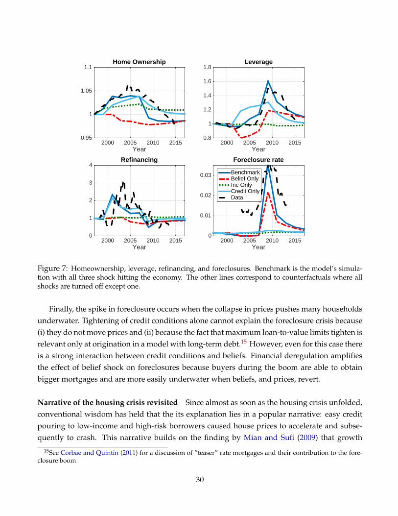
Leverage, refinancing and foreclosures The remaining panels of Figure 7 show the model’simplications for the dynamics of leverage, refinancing, and foreclosures over the boom andbust. Mechanically, the belief shift induces a fall in leverage (housing debt/housing value)during the boom, and a rise during the bust, simply because the denominator of leverage ischanging. Changing credit conditions cause an expansion of leverage during the boom anddeleveraging during the bust. It’s therefore, once again, the combination of the two shocks thatallows leverage to be flat in the boom, consistent with the US data. It’s also important to notethat the aggregate debt-to-income ratio increases dramatically in the model, as in the data, sinceleverage is constant and house prices grow four times more than income.
The change in credit conditions entirely accounts for the rise and fall in cash-out refi’s. It isthe decline in the fixed origination cost that, by shrinking the inaction region, induces signifi-cant growth in the number of households who choose to refinance their mortgage.
29
Year2000 2005 2010 2015
0.8
1
1.2
1.4
1.6
1.8Leverage
Year2000 2005 2010 2015
0
1
2
3
4Refinancing
Year2000 2005 2010 2015
0
0.01
0.02
0.03
Foreclosure rate
BenchmarkBelief OnlyInc OnlyCredit OnlyData
Year2000 2005 2010 2015
0.95
1
1.05
1.1Home Ownership
Figure 7: Homeownership, leverage, refinancing, and foreclosures. Benchmark is the model’s simula-tion with all three shock hitting the economy. The other lines correspond to counterfactuals where allshocks are turned off except one.
Finally, the spike in foreclosure occurs when the collapse in prices pushes many householdsunderwater. Tightening of credit conditions alone cannot explain the foreclosure crisis because(i) they do not move prices and (ii) because the fact that maximum loan-to-value limits tighten isrelevant only at origination in a model with long-term debt.15 However, even for this case thereis a strong interaction between credit conditions and beliefs. Financial deregulation amplifiesthe effect of belief shock on foreclosures because buyers during the boom are able to obtainbigger mortgages and are more easily underwater when beliefs, and prices, revert.
Narrative of the housing crisis revisited Since almost as soon as the housing crisis unfolded,conventional wisdom has held that the its explanation lies in a popular narrative: easy creditpouring to low-income and high-risk borrowers caused house prices to accelerate and subse-quently to crash. This narrative builds on the finding by Mian and Sufi (2009) that growth
15See Corbae and Quintin (2011) for a discussion of ”teaser” rate mortgages and their contribution to the fore-closure boom
30

30 40 50 60−0.06
−0.04
−0.02
0
0.02
0.04
0.06
Age
Log−
chan
ge (
rela
tive
to m
ean)
Boom
30 40 50 60−0.08
−0.06
−0.04
−0.02
0
0.02
0.04
Age
Log−
chan
ge (
rela
tive
to m
ean)
Bust
DataModel
Figure 8: Change in home ownership by age group in the data and in the model.
in purchase-mortgage originations at the ZIP code level turned from positively to negativelycorrelated with per-capita income in the run-up to the financial crisis, particularly in regionswith strong house appreciation. As a consequence of these empirical findings, much promi-nence has been given to the role of financial deregulation in channeling credit to low-incomeand subprime borrowers and in causing the boom-bust in house prices and consumption.
Our model speaks against this interpretation. Instead, our findings are consistent with anew narrative of the crisis that has recently emerged, thanks to the availability of new andmore refined micro data. According to several authors (Adelino et al., 2016; Albanesi et al., 2016;Foote et al., 2016), credit growth during the boom was not concentrated among the low-incomeand high-risk households but was a lot more widespread across the household distribution,and even reached high-income and prime borrowers. The top-left-panel of Figure 9, from Footeet al. (2016), shows that growth in the stock of mortgage debt over the boom occurred at similarrates across the whole household income distribution. The top-right panel replicates this figurein our model. The bottom-left panel reports mortgage originations by FICO score over the boomfrom Adelino et al. (2016): growth in mortgage debt is uniform across credit risk category. Ourmodel has no immediate counterpart of a credit score, but for each borrower we can computea probability of default at origination (embedded in the effective interest rate paid on debt, seeequation 6) and group households by risk level. The bottom-right panel of Figure 9 shows thatour model predicts fairly even credit growth between low-risk and high-risk borrowers.
In light of our analysis of the economic forces at work in the model, it is not surprising thatour simulated cross-section of debt growth lines up well with its empirical counterpart. In themodel, aggregate housing demand rises because all households – rich and poor, prime and sub-prime – expect large capital gains from holding this asset. High-income, low-risk households,
31

0.1
.2.3
.4.5
Sha
re o
f Deb
t
1 2 3 4 5
Income Quintile of Household
Shares of Mortgage Debt
2001 2007
0.2
.4.6
.8S
hare
of D
ebt
Above Median Below Median
Default Risk
Shares of Originated Mortgage Debt
2001 2007
Figure 9: Top-left panel: Share of mortgage debt by income level in 2001 and 2006 from Foote et al.(2016). Top-right panel: Share of mortgage debt by income level in the model in 2001 and 2007. Bottom-right panel: Share of mortgage originations by FICO score from Adelino et al. (2016). Bottom left panel:Share of mortgage originations by individual probability of default.
who are already in a position to access low-cost credit even without looser loan-to-value con-straints, are among those who choose to increase the housing share in their portfolio to takeadvantage of expected appreciation.16
Whose beliefs matter? Our rational expectations approach to modeling a belief shock im-poses that all agents in the economy share the same beliefs about future house prices, as well asthe same preferences over housing services and beliefs about future preferences. Thus, whenthe belief shock hits there are three channels through which the shock affects behavior. First,
16Interestingly, this is exactly the interpretation given by the authors uncovering these new facts. Adelino et al.(2016) (page 32) write that this suggests that demand-side effects and possibly also expectations of future house prices in-creases could have been important drivers in the mortgage expansion as borrowers and lenders bought into expected increasesin asset values. Foote et al. (2016) (page 35) conclude that their findings are more consistent with an alternative story, inwhich exogenous borrowing constraints play no role and the causality runs from house prices, or house-price expectations, tothe widespread accumulation of mortgage debt. During the boom, optimistic views of house-price growth were widely sharedby potential home buyers (in all income classes) as well as mortgage lenders.
32

individual households believe that they themselves are likely to desire more housing servicesrelative to non-durable consumption in the future. Since there are adjustment costs on housing,this may lead them to change their housing demand immediately, even in the absence of anychange in house prices. Second, individual households believe that all other households arelikely to desire more housing services relative to non-durable consumption in the future, andrationally foresee that this may lead to increase in the price of housing in the future. Thus ahousehold may be tempted to change their demand for housing due to a speculative motive,even if their own preferences are not affected by the change. Third, the financial sector un-derstands the implied dynamics for house prices and hence lenders change the optimal creditcontracts that they offer to home owners. These changes in lending contracts may also affecthouseholds’ demand for housing.
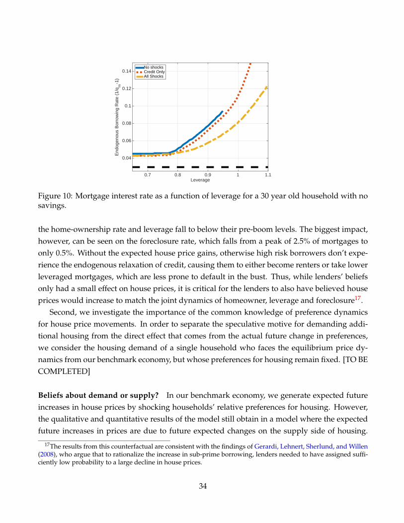
First, we investigate the role of the lenders’ beliefs. In Figure 10, the endogenous borrowingrate (the inverse of the price of a unit of mortgage debt, a function of the individual characteris-tics that predict default) in different aggregate states is plotted for a 30 year old household thatowns a $150K house and earns median income. The blue line is before any financial deregula-tion and in the absence of a belief shock. The maximum LTV that a household can take out is0.85. Note that for low levels of leverage the interest rate is flat, but starts increasing steadilyabove leverage of about 0.7. The green line shows that the belief shock flattens the q functionin the boom. The lenders have the same expectations as households: they also expect prices torise. Thus, they expect the probability of default to fall, and as a result they offer more favorablecredit conditions to all borrowers, but especially to the risky ones, who now become a lot saferin the eyes of the lender (the gap between the blue and the green line widens more for highLTVs). Thus, viewed through the lens of our model, the increased credit flow to riskier borrow-ers was an endogenous response to an increased belief in expected house price appreciation.
In order to quantify the importance of lenders’ beliefs in explaining the aggregate dynamicssurrounding the boom-bust episode, we consider a counterfactual economy where lenders donot share the same beliefs about house price appreciation as the households. Specifically, weassume that the banks place zero probability on transitioning to ϕ∗
L or ϕH, so that the forecasteddefault probabilities do not take into account expected future house price growth. We solve forthe new equilibrium of this economy with ”pessimistic” lenders.
When simulating the same boom-bust episode in the pessimistic lender economy, we findthat the lender’s beliefs only have a modest effect on the dynamics of house prices and non-durable consumption: house prices and consumption rise about 5 and 0.3 percentage pointsless, respectively. The lenders pessimistic beliefs, however, have a large impact on homeowner-ship, leverage and foreclosure. Contrary to the benchmark economy, when the belief shock hits
33
Leverage0.7 0.8 0.9 1 1.1
End
ogen
ous
Bor
row
ing
Rat
e (1
/qm
-1)
0.04
0.06
0.08
0.1
0.12
0.14No shocksCredit OnlyAll Shocks
Figure 10: Mortgage interest rate as a function of leverage for a 30 year old household with nosavings.
the home-ownership rate and leverage fall to below their pre-boom levels. The biggest impact,however, can be seen on the foreclosure rate, which falls from a peak of 2.5% of mortgages toonly 0.5%. Without the expected house price gains, otherwise high risk borrowers don’t expe-rience the endogenous relaxation of credit, causing them to either become renters or take lowerleveraged mortgages, which are less prone to default in the bust. Thus, while lenders’ beliefsonly had a small effect on house prices, it is critical for the lenders to also have believed houseprices would increase to match the joint dynamics of homeowner, leverage and foreclosure17.
Second, we investigate the importance of the common knowledge of preference dynamicsfor house price movements. In order to separate the speculative motive for demanding addi-tional housing from the direct effect that comes from the actual future change in preferences,we consider the housing demand of a single household who faces the equilibrium price dy-namics from our benchmark economy, but whose preferences for housing remain fixed. [TO BECOMPLETED]
Beliefs about demand or supply? In our benchmark economy, we generate expected futureincreases in house prices by shocking households’ relative preferences for housing. However,the qualitative and quantitative results of the model still obtain in a model where the expectedfuture increases in prices are due to future expected changes on the supply side of housing.
17The results from this counterfactual are consistent with the findings of Gerardi, Lehnert, Sherlund, and Willen(2008), who argue that to rationalize the increase in sub-prime borrowing, lenders needed to have assigned suffi-ciently low probability to a large decline in house prices.
34

We consider the same three state belief structure, but instead of changing the preference pa-rameter ϕ, we assume that what changes is the future size of land permits made available tothe construction company from the government. Thus, the boom is generated by householdsbelieving that less land will be made available for construction in the future18. Thus, we remainsomewhat agnostic as to the underlying fundamental shock which causes the increase in houseprices. However, what is important is that it operates through future expected house pricegrowth in order to jointly match the dynamics of housing investment19 and consumption in thedata.
Movements in the risk-free rate One other candidate explanation for the boom in houseprices was the dramatic decline in the risk-free rate experienced in the US in the 2000s. Wedid not consider this shock in our benchmark because, while it has the potentially to success-fully explain the housing and consumption boom, real interest rates have not risen again topre-2000 levels, making it difficult for them to be instrumental in the bust. In order to evaluatethis additional possible channel, we resolve our economy with an exogenous, but stochasticreal rate. For computational tractability, we then make the financial deregulation and produc-tivity shocks perfectly correlated. We assume that the real rate falls 100 basis points in 2001 andstays low through 2020. The impulse responses from this experiment are provided in the ap-pendix. The drop in the interest rate does yield larger movements in house prices in the boom,but qualitatively, the joint dynamics are very similar to the benchmark.
Sensitivity to Belief Process We perform a sensitivity analysis on the values of the transitionmatrix for the belief shock and the size of the shock. In the benchmark ϕH − ϕL = 0.08, as asensitivity we consider a 50% smaller movement, i.e. ϕH − ϕL = 0.04. The time series for houseprices is plotted in figure 11 as the green line with diamonds. The increase in house pricesis about 40% smaller, implying there is some non-linearity. The rent-price ratio falls by 12%instead of 16%, implying that the effect on expected future house prices gains is still strong evenwith the lower value for ϕH. The next sensitivity is lowering the persistence of ϕHH from 0.95to 0.8.20 The increase in house prices (the red line with circles) is about 2/3 of the benchmark,and the decline in the rent price ratio is similar to sensitivity to the size of the shock. That thechange to the persistence of the high state and the level give similar results is unsurprising,
18It is important that we maintain the structure of a shock to future availability of land. While decreasing theland available contemporaneously would lead to an increase in prices, it could lead to a counterfactual drop inhousing investment (similar to the counterfactual drop in consumption for the demand shock in the benchmark).
19This point has similarly been made in Berger et al. (2015).20ϕHL∗ = ϕHL = 0.1 in this case.
35

Year2000 2005 2010 2015
0.8
0.9
1
1.1
1.2
1.3
House Price
Benchmarkφ
H sense
qHH
sense
qL
*H
sense
Year2000 2005 2010 2015
0.95
1
1.05
1.1Consumption
Year2000 2005 2010 2015
0.65
0.7
0.75
0.8
0.85
0.9
0.95
1
1.05
1.1
1.15
Benchmarkφ
H sense
qHH
sense
qL
*H
sense
Figure 11: House price and rent price ratio. Benchmark is the model’s simulation with all three shockshitting the economy. The other lines correspond to sensitivities to the belief shock process
since they both reflect the expected size/duration of the preference shock. Finally, we performsensitivity on ϕL∗H, the probability of the demand shock realizing conditional on being in stateL∗. We consider cutting this probability in half, from 0.80 to 0.4.21
4.2 How does the fall in house prices transmit into consumption?
To understand the transmission mechanism from house prices to consumption expenditures inthe model, we analyze how the drop in household consumption during the bust (from 2007 to2011) correlates with initial leverage and the initial housing share of net wealth in 2007. Lever-age is computed as total debt divided by net wealth (including human wealth, computed asthe expected discounted present value of future after-tax earnings and social security benefits),and the housing share of net wealth is computed as housing equity divided by net wealth. Ifforced deleveraging (the collateral effect) is a strong force in the model, one should expect lever-age (the debt share of net wealth) to be negatively correlated with the change in consumption.Whereas, if the transmission mechanism if mainly through a wealth effect, one should expectthe change in consumption to be negatively correlated with the housing share of net wealth.
Figure 12 shows that leverage and the change in consumption are uncorrelated, whereashouseholds with the largest housing share are those with the largest drop in expenditures, anindication that they key channel of transmission in the model is a wealth effect. Note that
21We then set ϕL∗L = 0.1 and ϕL∗L∗ = 0.5.
36

−.4
−.3
−.2
−.1
0.1
Cha
nge
in L
og C
onsu
mpt
ion
2007
−20
11
0 .05 .1 .15
Total Debt as a fraction of Total Wealth
Renters Owners
−.4
−.3
−.2
−.1
0.1
Cha
nge
in L
og C
onsu
mpt
ion
2007
−20
11
0 .1 .2 .3 .4
Housing Share of Total Wealth
Renters Owners
Figure 12: Consumption drop during the bust (2007-2011) in the model plotted with respect to house-hold leverage (left panel) and housing share of net wealth (right panel).
renters have a small, but positive, change in consumption as a result of the equilibrium dropin rents. When we split the sample between workers and retirees, the contrast is even starkerfor workers – the plot for leverage remains flat, but the negative wealth effect is much morepronounced. The reason is that, in the model, retirees have an active luxury-bequest motiveand by adjusting their bequest can dis-save to smooth consumption.
4.3 Policy experiment: a debt forgiveness program
We now use the model to run a counterfactual policy experiment. We implement a massivedebt relief program in the model — a policy intervention that a number of economists andpolicy-makers thought could have cushioned the housing crash and accelerated the recoveryin aggregate expenditures. All homeowners with more than 95 percent LTV ratio see their ex-cess debt forgiven, with the government stepping in and reimbursing the banks. The residualmortgage is paid off by households under the baseline amortization formula. This principalreduction program is implemented in 2009, it is unexpected and households do not believethat such a program will ever be implemented again in the future. Overall, the counterfactualprogram affects around 1/4 of all mortgagors, i.e. it displays a much larger scale (and a bet-ter timing) than the programs, such as HAMP (Home Affordable Modification Program) andHARP (Home Affordable Refinance Program), initiated by the Obama administration.
Figure 13 shows that the program is very effective in cutting the number of underwaterhouseholds and in reducing foreclosures. Thus, to the extent that foreclosures imply a utilityloss and accelerated depreciation of the property, there is a gain for the households and bankswho can avoid it. Leverage, mechanically rises less. However, the effect on house prices andconsumption is trivial. First, by limiting foreclosure and the associated large depreciation, thesupply of housing goes up. This, in turn, pushes the price per unit of housing down (an unin-tended consequence of the policy). Second, foreclosure is an insurance vehicle for consumption
37

Year2000 2005 2010 2015
0.8
1
1.2
House Price
Bench.Mod.
Year2000 2005 2010 2015
0.95
1
1.05
1.1Consumption
Year2000 2005 2010 2015
0
0.01
0.02
0.03
Foreclosure rate
Year2000 2005 2010 2015
0.8
1
1.2
1.4
1.6
Leverage
Figure 13: House prices, aggregate consumption, foreclosures and leverage. The dashed linecorresponds to the debt forgiveness program.
smoothing. By limiting foreclosures, those households who now do not foreclose, but wouldhave in absence of the policy, consume less. It is only the households with high LTV ratios thatwould not have foreclosed who now have lower mortgage payments and consume more. Thesebeneficiaries of the policy, though, account for a relatively small share of aggregate consump-tion. These results are consistent with the empirical findings of Agarwal et al. (2012) who usea diff-diff approach to evaluate the effects of HAMP and document that the regions where thepolicy was used most intensively experienced no change in non-durable consumption22.
The results of this policy counterfactual also highlight how in the model, as in the data,leverage increased throughout the income distribution. Even households who were not un-derwater after the bust still had a desire to deleverage (mostly by simply paying down themortgage as prescribed by amortization). This slow deleveraging by the bulk of homeownersis behind the tepid consumption recovery following the bust and explains why the proposedinterventions have had a limited impact in speeding the recovery in consumption and houseprices.
22Studying the HARP program, Mitman (2016) finds small effects on foreclosure and modest effects on con-sumption for households who were able to refinance under the program
38

5 Implications for the elasticity of consumption to house prices
A vast empirical literature in economics tries to estimate, with household-level longitudinaldata (Campbell and Cocco, 2007; Browning et al., 2013), geographical-level panel data (Mianet al., 2013), or time-series data (Carroll et al., 2011) the elasticity of consumption expendituresto changes in house prices. This literature is, however, plagued by the ’comovement problem’.First, the endogeneity of house prices makes it extremely challenging to find exogenous sourcesof variation in the data that can identify correctly the parameter of interest. Second, even underthe best identification scenario, we argue that measuring the response of consumption to an’exogenous’ change in house prices is not especially relevant, since it is an event that doesnever occur in practice. Since prices are an equilibrium object, house prices changes are neverexogenous. Rather, house price changes are the result of the realization of some combinationof underlying shocks that influence either the demand or supply of housing, or both, and thuscause equilibrium house prices to move.
This distinction is important only if the elasticity of aggregate consumption to house pricesvaries a lot depending on the many possible macroeconomic shocks that lead to house pricemovements. With our structural equilibrium multi-shock model in hand, we are in the best po-sition to answer this question. Table 4 reports the time series elasticity of aggregate nondurableconsumption expenditures to house prices computed by simulating the model under four pos-sible sources of price dynamics: productivity, financial deregulation, beliefs, and preferences.Elasticities are computed for both the boom and the bust.
Our main result is that these elasticities are remarkably different across shocks. Incomeshocks generate the largest elasticities of consumption to house prices, well above one, as in-come shocks are quite persistent and affect consumption directly, not just through their effectthrough house prices. The elasticities induced by shocks to the taste for housing are, instead,negative: households with an increased preference for housing spend more on housing and lesson nondurable consumption. The relaxation of collateral constraints is associated to a negativeelasticity of consumption to house prices, because a number of households can now afford tobuy a house and cut expenditures to finance the required down payment. Finally, the beliefshock induces a moderate response of consumption to house prices: many homeowners stayin their house and extract more equity to increase consumption. At the same time, this force iscounteracted by the fact that other households upgrade their housing and, in the process, limittheir consumption expenditures in order to meet the larger down-payment requirement andthe transaction costs.
These results have implications for the use of the sufficient statistic approach (as advocated,
39

Boom BustTotal 0.24 0.25
Productivity 1.60 1.28Credit conditions −0.61 0.32Belief shift 0.15 0.18
Taste for housing −0.28 −0.23
Table 4: Elasticities of Nondurable Consumption to House Prices during the Boom and the Bust.Results of counterfactuals when a single shock affects house prices.
for example, in Chetty, 2008) to this question. In a recent paper, Berger et al. (2015) propose aclever and easy way to compute a ’sufficient statistic’ to estimate the individual (micro) elastic-ity of consumption to a permanent change in house prices. Their sufficient statistic amounts tothe product between the individual marginal propensity to consume out of a transitory incomeshock and her beginning-of-period quantity of housing.
The left panel of Figure 14 shows that their sufficient statistic, once aggregated across thepopulation, provides an excellent approximation to the true elasticity computed by simulatingdata from the model when the underlying shock is the belief shock, i.e., in the context of therecent boom-bust episode for which we argued that fluctuations in beliefs about future housingdemand account for much of house price dynamics. The reason is that the belief shock is largelyorthogonal to other determinants of consumption decisions, and thus it is akin to house priceshocks in housing-demand models where such prices are exogenous, as in the framework thatBerger et al. (2015) use to derive their sufficient statistic.
However, we also emphasize that one should exercise caution when using this approach:the sufficient statistic could fail quite dramatically in replicating the true elasticity, dependingon the shock underlying house price movements. The right panel illustrates one such starkexample when the source of fluctuations is shocks to the taste for housing. By design, thesufficient statistic is positive, whereas as shown in Table 4 the true elasticity is negative.
6 Conclusions
Equilibrium models with heterogeneous households, incomplete markets, and aggregate shocksare becoming a standard tool to analyze the macroeconomy and study the welfare and distri-butional consequences of government policy. In this paper we have built a rich version of thisframework to examine the co-movement between consumption and house prices around the
40
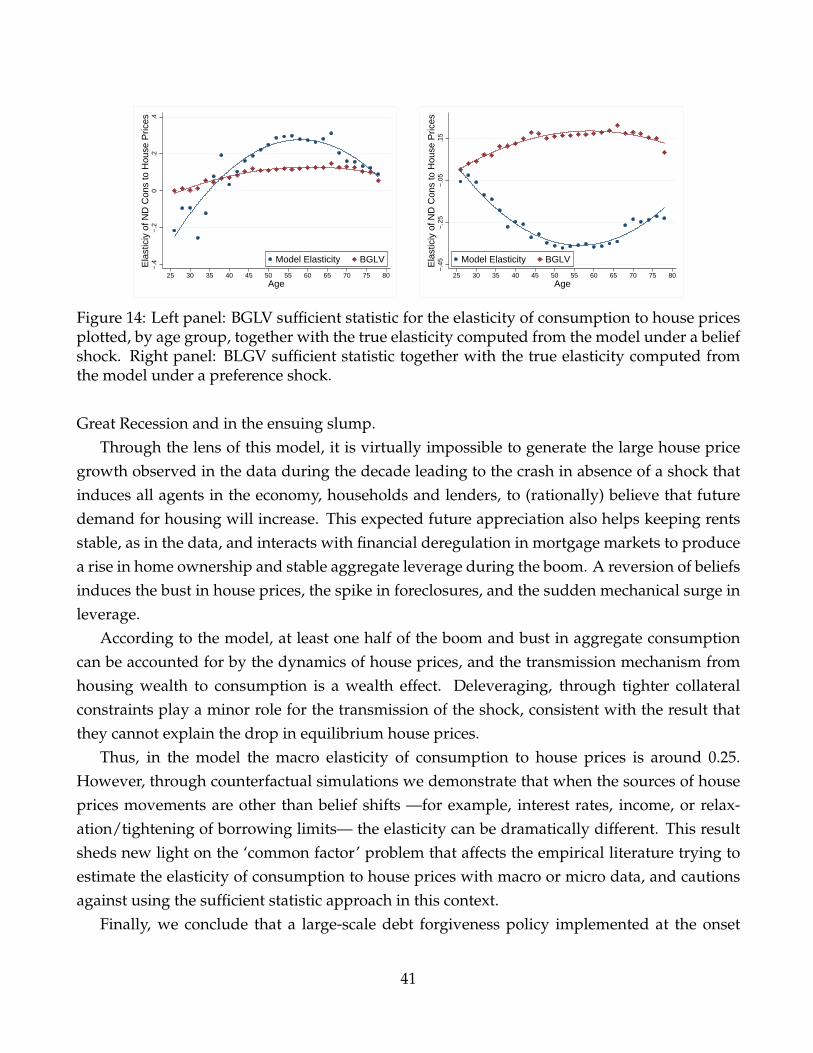
−.4
−.2
0.2
.4E
last
iciy
of N
D C
ons
to H
ouse
Pric
es
25 30 35 40 45 50 55 60 65 70 75 80Age
Model Elasticity BGLV
−.4
5−
.25
−.0
5.1
5E
last
iciy
of N
D C
ons
to H
ouse
Pric
es
25 30 35 40 45 50 55 60 65 70 75 80Age
Model Elasticity BGLV
Figure 14: Left panel: BGLV sufficient statistic for the elasticity of consumption to house pricesplotted, by age group, together with the true elasticity computed from the model under a beliefshock. Right panel: BLGV sufficient statistic together with the true elasticity computed fromthe model under a preference shock.
Great Recession and in the ensuing slump.Through the lens of this model, it is virtually impossible to generate the large house price
growth observed in the data during the decade leading to the crash in absence of a shock thatinduces all agents in the economy, households and lenders, to (rationally) believe that futuredemand for housing will increase. This expected future appreciation also helps keeping rentsstable, as in the data, and interacts with financial deregulation in mortgage markets to producea rise in home ownership and stable aggregate leverage during the boom. A reversion of beliefsinduces the bust in house prices, the spike in foreclosures, and the sudden mechanical surge inleverage.
According to the model, at least one half of the boom and bust in aggregate consumptioncan be accounted for by the dynamics of house prices, and the transmission mechanism fromhousing wealth to consumption is a wealth effect. Deleveraging, through tighter collateralconstraints play a minor role for the transmission of the shock, consistent with the result thatthey cannot explain the drop in equilibrium house prices.
Thus, in the model the macro elasticity of consumption to house prices is around 0.25.However, through counterfactual simulations we demonstrate that when the sources of houseprices movements are other than belief shifts —for example, interest rates, income, or relax-ation/tightening of borrowing limits— the elasticity can be dramatically different. This resultsheds new light on the ‘common factor’ problem that affects the empirical literature trying toestimate the elasticity of consumption to house prices with macro or micro data, and cautionsagainst using the sufficient statistic approach in this context.
Finally, we conclude that a large-scale debt forgiveness policy implemented at the onset
41

of the housing crisis would have significantly reduced foreclosures, but it would have beenentirely ineffective in cushioning the fall in house prices or speeding up the recovery in con-sumption.
42

ReferencesADELINO, M., A. SCHOAR, AND F. SEVERINO (2016): “Loan Originations and Defaults in the Mortgage Crisis:
The Role of the Middle Class,” Review of Financial Studies, hhw018.
AGARWAL, S., G. AMROMIN, I. BEN-DAVID, S. CHOMSISENGPHET, T. PISKORSKI, AND A. SERU (2012): “PolicyIntervention in Debt Renegotiation: Evidence from the Home Affordable Modification Program,” Tech. rep.,National Bureau of Economic Research.
ALBANESI, S., G. DE GIORGI, J. NOSAL, AND M. PLOENZKE (2016): “Credit Growth and the Financial Crisis: ANew Narrative,” Tech. rep., Mimeo, Ohio State University.
BERGER, D., V. GUERRIERI, G. LORENZONI, AND J. VAVRA (2015): “House Prices and Consumer Spending,”Working Paper 21667, National Bureau of Economic Research.
BLUNDELL, R., L. PISTAFERRI, AND I. PRESTON (2008): “Consumption inequality and partial insurance,” TheAmerican Economic Review, 98, 1887–1921.
BROWNING, M., M. GØRTZ, AND S. LETH-PETERSEN (2013): “Housing wealth and consumption: a micro panelstudy,” The Economic Journal, 123, 401–428.
BURNSIDE, C., M. EICHENBAUM, AND S. REBELO (2011): “Understanding booms and busts in housing markets,”Tech. rep., National Bureau of Economic Research.
CAMPBELL, J. Y. AND J. F. COCCO (2007): “How do house prices affect consumption? Evidence from micro data,”Journal of Monetary Economics, 54, 591–621.
CARROLL, C. D., M. OTSUKA, AND J. SLACALEK (2011): “How large are housing and financial wealth effects? Anew approach,” Journal of Money, Credit and Banking, 43, 55–79.
CASE, K. E., J. M. QUIGLEY, AND R. J. SHILLER (2011): “Wealth effects revisited 1978-2009,” Tech. rep., NationalBureau of Economic Research.
CHATTERJEE, S. AND B. EYIGUNGOR (2013): “Debt dilution and seniority in a model of defaultable sovereigndebt,” Tech. rep., FRB of Philadelphia Working Paper.
CHETTY, R. (2008): “Sufficient statistics for welfare analysis: A bridge between structural and reduced-form meth-ods,” Tech. rep., National Bureau of Economic Research.
CORBAE, D. AND E. QUINTIN (2011): “Mortgage Innovation and the Foreclosure Boom,” Working Paper,University of Wisconsin.
DE NARDI, M., E. FRENCH, AND D. BENSON (2011): “Consumption and the Great Recession,” Tech. rep., NationalBureau of Economic Research.
FAVILUKIS, J., S. C. LUDVIGSON, AND S. VAN NIEUWERBURGH (2010): “The macroeconomic effects of housingwealth, housing finance, and limited risk-sharing in general equilibrium,” Tech. rep., National Bureau of Eco-nomic Research.
43
FOOTE, C. L., L. LOEWENSTEIN, AND P. S. WILLEN (2016): “Cross-Sectional Patterns of Mortgage Debt Duringthe Housing Boom: Stocks and Flows,” Tech. rep., Mimeo, Federal Reserve Bank of Boston.
GERARDI, K., A. LEHNERT, S. M. SHERLUND, AND P. WILLEN (2008): “Making sense of the subprime crisis,”Brookings Papers on Economic Activity, 2008, 69–159.
HEATHCOTE, J., F. PERRI, AND G. L. VIOLANTE (2010): “Unequal we stand: An empirical analysis of economicinequality in the United States, 1967–2006,” Review of Economic dynamics, 13, 15–51.
HEATHCOTE, J., K. STORESLETTEN, AND G. L. VIOLANTE (2014): “Optimal tax progressivity: An analytical frame-work,” Tech. rep., National Bureau of Economic Research.
IACOVIELLO, M. AND S. NERI (2010): “Housing Market Spillovers: Evidence from an Estimated DSGE Model,”American Economic Journal. Macroeconomics, 2, 125.
KAPLAN, G. AND G. L. VIOLANTE (2014): “A Model of the Consumption Response to Fiscal Stimulus Payments,”Econometrica, 82, 1199–1239.
KRUSELL, P. AND A. A. SMITH, JR (1998): “Income and wealth heterogeneity in the macroeconomy,” Journal ofpolitical Economy, 106, 867–896.
MIAN, A., K. RAO, AND A. SUFI (2013): “Household Balance Sheets, Consumption, and the Economic Slump,”The Quarterly Journal of Economics, 128, 1687–1726.
MIAN, A. AND A. SUFI (2009): “The Consequences of Mortgage Credit Expansion: Evidence from the US MortgageDefault Crisis,” The Quarterly Journal of Economics, 124, 1449–1496.
——— (2014): “What Explains High Unemployment? The Aggregate Demand Channel,” Tech. rep., mimeo,Princeton.
MITMAN, K. (2016): “Macroeconomy Effects of Bankruptcy and Foreclosure Policies,” American EconomicReview, 106.
PENNINGTON-CROSS, A. (2009): “The Value of Foreclosed Property,” Journal of Real Estate Research.
PETEV, I., L. PISTAFERRI, AND I. S. EKSTEN (2011): “Consumption and the Great Recession: An analysis of Trends,Perceptions, and Distributional effects,” .
PIAZZESI, M., M. SCHNEIDER, AND S. TUZEL (2007): “Housing, consumption and asset pricing,” Journal ofFinancial Economics, 83, 531–569.
44

Year2000 2005 2010 2015
0.98
0.99
1
1.01
1.02
1.03
1.04
1.05
BenchmarkWedge OnlyLTV OnlyPTI Only
Figure 15: Decomposing the effect of credit changes on homeownership.
7 Appendix
7.1 Alternative Shocks
7.1.1 Decomposing Credit Shock
7.1.2 Land Shock
7.1.3 Interest Rate
[To Be Completed]
45

Year2000 2005 2010 2015
0.8
0.9
1
1.1
1.2
1.3
1.4
1.5
1.6
1.7
1.8Leverage
Year2000 2005 2010 2015
0
0.005
0.01
0.015
0.02
0.025
0.03
0.035
0.04Foreclosure rate
BenchmarkWedge OnlyLTV OnlyPTI Only
Figure 16: Decomposing the effect of credit changes on leverage and foreclosure.
Year2000 2005 2010 2015
0.8
0.9
1
1.1
1.2
1.3
House Price
ModelData
Year2000 2005 2010 2015
0.95
1
1.05
1.1Consumption
Figure 17: House prices and aggregate consumption. Benchmark is the model’s simulation with allshocks hitting the economy. The other line represents only the shock to land availability.
46

Year2000 2005 2010 2015
0.8
0.9
1
1.1
1.2
1.3
House Price
Land ModelLand Only
Year2000 2005 2010 2015
0.6
0.8
1
1.2
Housing Investment
Figure 18: House prices and aggregate housing investment. Land model is the model’s simulation withall shocks hitting the economy. The other line represents only the shock to land availability.
47