Content Addressable Memory ProjectNASA NAG-2 668

Semiannual Progress Report (Sep91-Feb92)

Rutgers University

New Brunswick, NJ 08903

J. Hall (PI) S. Levy (PI) D. Smith K. Miyake

Laboratory for Computer Science Research

Department of Computer Science

March 1,1992

_iliv. ) L! ? : O-f,L ,"_ _7 JrlC 1 :,'=.

,,,, : _77

https://ntrs.nasa.gov/search.jsp?R=19920012970 2018-07-09T21:36:04+00:00Z

1 abstract

A parameterized version of the tree processor has been designed and tested (by simulation).

The leaf processor design is 90% complete. We expect to complete and test a combination

of tree and leaf cell design in the next period. Work has been proceeding on algorithms

for the CAM, and once the design is complete we will begin simulating algorithms for large

problems.

In the last 6 months we have produced four publications that describe various components

of our research. They are summarized below.

J. Storrs Hall, Donald E. Smith, and Saul Levy, The Practical Implementation of

Content Addressable Memory, LCSR-TR-179, Laboratory for Computer Science

Research, Rutgers University, March 92. This was also submitted to the 1992 Frontiers

of Massively Parallel Computation Conference.

LCSR-TR-179 presents a functional description of our CAM architecture and discusses

attributes(e.g., density, scalability, data-path width, and coupling) that determine the

effectiveness of such architectures. In addition, two examples are presented that demon-

strate the use of CAM-based algorithms.

Donald E. Smith, Keith M. Miyake, and J. Storrs Hall, Design of a LEAF cell for

the Rutgers CAM Architecture, LCSR-TR-180, Laboratory for Computer Science

Research, Rutgers University, March 92.

LCSR-TR-180 presents a specification of the LEAF cell and its interfaces to other

modules in the CAM architecture. It describes the four communicating processors

which compose each LEAF cell (i.e., k-bit, 1-bit, IO, and memory) and their respective

interfaces.

Keith M. Miyake, Donald E. Smith, Circuit Design Tool User's Manual, LCSR-

TR-181, Laboratory for Computer Science Research, Rutgers University, March 92.

LCSR-TR-181 describes the design tool we have implemented in support of CAM re-

search. The design tool is written for a UNIX software environment and supports the

definition of digital electronic modules, the composition of modules into higher level

circuits, and event-driven simulation of the resulting circuits. Our tool provides an in-

terface whose goals include straightforward but fiexible primitive module definition and

circuit composition, efficient simulation, and a debugging environment that facilitates

design verification and alteration.

The unique architectural aspects of the Rutgers CAM uses many of the features typical

to most design tools; however, it also requires some features that are not widely sup-

ported. Our design makes use of many similar, but not identical, modules which puts

a premium on design tools that support parameterized modules (e.g., generic entities

in VHDL) and strong typing of a module's ports. In addition, since our design is con-

tinually evolving, the quality of and control over error handling, in both the design as

well as the simulation phase, is very important. In looking for a design tool to support

our research we found that either some critical features were inadequately supported

or the tool was much more than we required. In response to this environment we im-

plemented a prototype design tool that supports exactly the features required by the

design of the CAM.

S. Wei and S. Levy, Design and Analysis off Efficient Hierarchical Interconnec-

tion Networks, LCSR-TR-167, Laboratory for Computer Science Research, Rutgers

University, September 91. A shorter version of this paper was published as: S. Wei

and S. Levy, Design and AnMysis off Efficient Hierarchical Interconnection

Networks, Proceeding of 1991 Supercomputing Conference, Nov. 91, pgs 390-399.

LCSR-TR-167 presents a new approach to message-passing architectures based on

the general idea of hierarchical interconnects. The approach chooses the appropriate

number of interface nodes and clusters based on performance and cost-effectiveness.

The report includes both static and queueing analyses of such networks.

March 92

THE PRACTICALIMPLEMENTATION OF CONTENT

ADDRESSABLE MEMORY*

J. Storrs Hall, Donald E. Smith,and Saul Levy

LCSR-TR-179

Laboratory for Computer Science Research

Hill Center for the Mathematical Science

Busch Campus, Rutgers University

New Brunswick_ New Jersey 08903

"This work was supported by the Defense Advanced Research Projects Agency

and the National Aeronautics and Space Administration under NASA-Ames

Research Center grant NAG 2-668.

The Practical Implementation of Content Addressable Memory

J. Storrs Hall

Don Smith

Saul Levy

The Rutgers CAM ProjectI

Laboratory for Computer Science Research

Rutgers University

Keywovds

content addressable memory, associative processors, SIMD, processor arrays

Abstract

The notion of using content addressable memory (CAM) to achieve massively parallel

processing has resurfaced regularly since it first appeared in the 1960's, but has consistently

failed to produce cost-effective general-purpose systems. An analysis of this situation

reveals a number of specific design pitfalls regarding memory density, scalabihty, datapath

width, and processor coupling. Once these are avoided, specific functionalities must be

included in the design. This paper details the pitfalls and presents an architecture which

avoids them. Further, guidelines are developed for estimating CAM's effectiveness as a

parallel processor.

1 Supported by DARPA and NASA under NASA-Ames grant NAG 2-668

Introduction

"Pure" content addressable memory (CAM), such as is used in cache lookup, is a

method of addressing where each word of memory has a variable address, explicitly stored

with the word. With every memory access, the desired address is compared with the

stored address in every word. We are concerned here with an extension of this concept

which forms the basis for a method of massively parallel processing. It dates back at

least to Falkoff[621 and has been called many things, including content addressable parallel

processing (Foster[76]) and associative computing (Potter[88]). We shMl use CAM as a

generic term, to include parallel processing, and will refer to "pure CAM" if it is necessary

to distinguish the simple form.

This paradigm is well explained in Foster[76]. The broadcast value, instead of being

compared strictl.y with the address portion of the word, is compared with the entire word

(with a mask to provide "don't care" bit positions). The result of the comparison, rather

than immediately causing a read or write of a matching word, is stored in an explicit

"response bit". The bit is then used to control subsequent read/write operations; in

particular, more than one word can be written into simultaneously. Boolean functions are

then synthesized from sequences of tests, and bit-serial aithmetic can be performed on all

words in parallel.

At a higher level, the model allows for logic, comparisons, and arithmetic between some

global value and a local value stored in each word, or between local values in each word.

Individual words may refrain from the operations based on locally determined conditions.

This results in an architecture which is equivalent to a SIMD star network, with the CPU

as the hub and each word as a leaf processor. Since the hardware in the memory is only a

few gates in addition to a flip-flop at each bit, CAM should, or so the theory goes, form

the basis for massively parallel processors at densities near those of static RAMs.

We examine two questions: (a) can CAM (or some mechanism that implements the

CAM computational model) really be built within a small constant factor in cost of RAM,

and (b) if so, how efficiently can it be used?

Typical implementations of CAM

This section explains how, starting from the basic idea of CAM, a designer might

ultimately end up with any of a number of existing processor array architectures. This is

not to be taken to imply that any of those systems were designed that way, nor indeed had

the CAM model in mind at all. It does, however, fairly reflect the authors' own attempts

to find a cost-effective realization of the paradigm.

The first problem the CAM designer meets is that CAMs useful for parallel processing

require very wide words-256 bits is not unreasonable. Furthermore, each bit position

requires a data line and a mask line in the bus, doubling its width. Requiring a 512-bit

wide bus is not impossible, but the CAM also requires a connection between each bit in

any given word, which ordinary memory does not. Thus it is problematical to spht CAM

memories onto separate chips, requiring the pinouts of each chip to handle the entire buswidth.

What is worse, in the process of most CAM operations, a large portion of the bus is

wasted. Most comparisonsare of smaller fields within a word (selected by the mask lines),

and in the case of the bit-serial, word-parallel arithmetic, only one or two bits are being

tested or set at a time! Clearly, an optimization can be performed: all the comparators

at each bit can be removed, and in their place a one-bit ALU can be added to the word.

The "match" daisy chain and the read/write control lines can be replaced with a one-bit

local bus running across the word. Now the (global) bus is much smaller: an opcode for

the ALU, a bit address which can be decoded on-chip, a one-bit data bus. What is more,

arithmetic is faster; single-bit arithmetic operations are built into the ALU rather than

being synthesized out of logic operations which are in turn synthesized out of masking and

testing.

At this point there is a strong temptation for the designer to split the architecture

across chips, having processor chips which connect to standard memory chips. This has

the advantage of making memory much less expensive, but the disadvantage of tying the

number of words to the pinout of the processor chip. The relationship to the original CAM

paradigm begins to become somewhat strained also; this implementation puts a strong

downward pressure on the number of words/processing elements, and a strong upward

pressure on PE complexity, inter-PE connectivity, etc. In practice, this has been the

best tradeoff point for CAM-like implementations; it characterizes the evolutionary niche

occupied by the CM-1, the DAP, the MPP, and even the Illiae. Of course these machines

were not (necessarily) designed as an implementation of CAM: they are mentioned to

illustrate the point in the design space toward which CAM tends to gravitate.

We should mention, as a counterpoint, the STARAN (Batcher[T4]), which was de-

signed to implement CAM ideas. STARAN consisted of a number of 256-word arrays of

25f-bit words. Today a STARAN array could be put on a single chip, but there would

still be the bus to contend with. Perhaps predictably, the major thrust in CAM-like

architectures in the interim has been along the processor-array "lines.

Criteria

Given these facts, it behooves the architect of a CAM-based system to develop a very

strong theory of why the CAM paradigm has failed to produce a cost-effective general-

purpose architecture. Here is the theory:

o Density: The basic CAM algorithms are based on the assumption that all of the

memory in the system is CAM. No implementation to date has come near this. CAM

has been a scarce commodity, backed up by RAM, and data is swapped in and out

of CAM to be processed. This is deadly, since CAM at best transforms a linear

search or other simple loop to a constant-time operation; swapping the data in or out

re-introduces the linear time.

o ScaJability: For physical practicality, CAM chips must have constant pinout, indepen-

dent of the number of words per chip. The size of ordinary RAM is an extraordinarily

scalable feature of the von Neumann architecture, varying by more than six orders

of magnitude over the range of different systems. If CAM is not also scalable in this

very strict sense, it will fail to substitute for RAM.

o Datapath width: In choosing a one-bit processor, a CAM implementation gains faster

arithmetic but loses content addressability. If comparisonsare bit serial, CAM isslower than conventional indexing structures such as binary trees and hash tables. To

be usable as CAM, a memory must be able to compare, add, and subtract in a time

comparable to a normal memory access.

Coupling: The overwhelming tendency in designing a SIMD processor array is to

place it as an attached processor to some conventional machine which manages the

data not being used in the current parallel computation. This is unworkable; the

bottleneck means that unless there are large speedups to be gained from operations on

relatively long-lived data, the serial host processor can perform most simple associative

operations faster than the CAM, when the time to transfer the data to and from the

attached processor is taken into account.

Density

Perhaps the most important criterion is density. The CAM must be usable as mem-

ory. If this is met, the basic CAM algorithms can be brought into play. Associative

retrieval allows arrays of simple, explicitly-indexed records to be used instead of trees,

linked lists, hash tables, priority queues, and inverted indices; what is more, it saves the

software designer from having to make choices, with their associated tradeoffs, between

these structures. (See Hall[81], Potter[88].)

It would be extremely inefficient to use a "true" parallel processor for search opera-

tions. The algorithmic speedup is at best Io 9 N, so its efficiency is _N , e.g. 0.002% in the

case of a million-word CAM. Luckily, as distinct from "pure" CAM, the parallel processing

CAM model produces significantly better speedups for other operations. If a million-word

CAM has the same hardware cost as a fully-connected parallel l_rocessor with a thousand

nodes, the CAM need only achieve an average 0.1% speedup to equal, in operations per

cycle, the true parallel processor with perfect 100% linear speedup. (Caveat: A whole-chip

processor will almost certainly have faster cycles than a CAM.)

Even so, we would llke to keep the CAM to within some small constant factor of RAM

cost. While a somewhat speculative analysis indicates that CAM might be rated as having

a processing power proportional to the square root of the number of words, it remains the

case that in order to do so it must act as the system's primary memory. Thus, its cost must

remain low independent of the processing power it provides. This can be accomplished by

starting with a high-density DRAM design and only allowing some constant fraction of

the chip to be used for the active elements that implement the CAM model.

Scalability

The only interconnection schemes that meet the strict scalability criterion are a bus,

a linear array (daisy chain), and a tree. We find that a bus is desireable to distribute

instructions to the words; a tree is essential for implementing the collective functions the

CAM computational model requires; and a long shift register is probably the best way

to implement an asynchronous I/O capability that does not seriously interfere with other

operations.

Width

Consider the following design task: you have 1024 full adders and desire to build a

machine to compute 1024 evenly spaced points of a linear function y = mz + b in 32-bit

fields. You can add whatever control, memory, and communications you like. There are

three strategies:

¢ First, you could make a serial processor using all the hardware to form a circuit that

could multiply in one cycle. Then loop computing ms + b at each iteration, taking

2048 cycles. This can be improved by a strength reduction optimization, starting with

b and adding m at each iteration, for a total of only 1024 cycIes.

o Second, use 1024 1-bit ALUs to compute the result directly, multiplying in each pro-

cessor mi (where i is the processor number stored as a constant) and adding b, taking

1024-t-32 = 1056 cycles. This is better than the naive serial algorithm but comparable

to the optimized one.

o Third, one can form 32 32-bit ALUs and take advantage of parallelism and strength

reduction: in a 32-cycle multiply (and a 1-cycle add), form the number 32im + b at

each processor (where 32i has been stored as a constant) and use that as a starting

point for adding m for the next 31 points. This gives you a total of 64 cycles.

This example is illustrative of a class of algorithms, which we call semi-serial algo-

rithms, for which ALUs of a width commensurate with the data of interest and capable

of simple arithmetic and comparison, but not more, form a local optimum in hardware

efficiency. Note that for large problems using a fixed algorithm, the three designs above

are equivalent: each can do 1024 multiplies in 1024 cycles.

Coupling

Having attained memory-like density in the CAM, we can use it to advantage by the

simple expedient of replacing all the system's RAM with CAM. (An alternative approach

would be to use a Harvard-like architecture with RAM for instruction memory and CAM

for data memory.) It is a long-established trend for processors to be faster than memory

and to run asynchronously. In practice, this may mean that special processors are not

necessary for CAM-based systems (although it is certainly possible to design them).

In a RAM, where only one word is being accessed at a time, clock skew across the

memory is not a serious problem. In a CAM, it might be. If the connectivity is a tree, out-

going information, i.e. from the CPU to the CAM may arrive at the memory in a skewed

fashion harmlessly, since no leaf depends on information from any other leaf. However,

ingoing information may need to be synchronized. If the ingoing datapaths are combi-

national, synchronization consists only of waiting the longest number of gate delays from

CAM to CPU. If the delay is consistent, this is not only simpler but faster than any othermethod.

Other Feature_

To be effective as CAM, a system must not only avoid these pitfalls but be designed

with a cognizance of typical CAM algorithms in order to make most efficient use of its

hardware. The following is a list of features we have found to confer substantial algorithmic

advantages, while remaining implementable within the constraints above:

o Collective functions: The CAM model is virtually useless without a fairly powerful

feedback mechanism from the memory to the processor. After an associative search,

the processor may need to know how many (if any) matches were found. In the classical

CAM model, operations such as summing all active words, finding the maximum

or minimum of a set of values, and the like can be done as word-parallel bit-serial

algorithms. These operations are crucial parts of the basic CAM computational model.

o Segmentation: The CAM model has the capability of doing in parallel essentially a

simple loop, dealing only with local and global values at each point. The ability to

segment the CAM, still doing the same operation everywhere but having a different

"global" value in each segment, corresponds to doing nested loops, and extends the

range of parallel operations significantly:

o Local addressing: The fields of the CAM words which are going to be operated on by

an instruction are, in the basic model, the same for each word. The ability to vary

the field choice on the basis of local data allows the CAM to do things llke regular

expression matching or unification in parallel, a prerequisite to the extension of the

ideas of content addressability into higher-level models of computation.

The Rutgers CAM

At this point we shift terminological gears; the specifics of the model are enough more

complex that the concept of a "word" splits into two separate terms: a "cell" is the locus of

one active element and the unit of activity control; the term "word" hereinafter will mean

an addressable unit of simple memory whose width is that of the_bus and other datapaths.

There are many words per cell.

The design criteria elucidated in the preceding sections interact strongly with par-

ticular states of technology to determine the viability of a CAM implementation. As a

point of departure, let us assign values to the constants as follows: Word width, 32 bits;

density, 1K words per ALU. With these parameters we can devote at least half the silicon

to DRAM; the density of the CAM a, memory will be at least half that of conventional

memory in the same technology.

A decade ago, the dominant memory technology was 64 K-bit DRAMs. The above

constraints would specify a 32 K-bit chip, with one ALU occupying half the space and 1K

32-bit words on the other half, for a total of one cam cell per chip. A one-megabyte memory

(typical for mainframes of the day) would have consisted of 256 chips (and therefore 256

cam cells). Assuming the CAM could be driven at 5MHz and do one operation every 5

cycles, the CAM would have represented a 256 mega-ops peak processing rate.

For the mid-90's we can use a 64-Meg DRAM as a basis and obtain 1K cam cells per

chip. (Each cell is still an ALU and 1K 32-bit words; the memory still occupies half the

chip.) 16 chips would provide 64 megabytes of memory and, assuming a 10-MHz operations

rate (from a 50-MHz system clock), a peak 160 giga-ops. This is a single-board computer.

We have developed a "CAM virtual machine '_ as a common focus for architectural

and algorithmic efforts. This model of the CAM reflects the capabilities of active elements

which fit the tradeoffs above,i.e. all the circuitry associatedwith one CAM call must beroughly the sizeof 1K words of DRAM.

The CAM model is related to Blelloch's[87] "scan model of computation", but differs

in the fundamental regard that the CAM model does not have a general permutation

operator and thus is not a complete modal for paralld computation. It does include:

o Activity control: all the following can be controlled on a per-cell per-instruction basis.

This forms the major difference between CAM and simple vector styles of computation.

o Parallel vector operations to include addition, subtraction, comparison, bitwise bool-

ean functions, and some shifting and byte extraction. These operations can only be

done between words of the same cell, but they need not be the same words in each

cell. It does not include multiplication, division, or floating point, although these can

be done in software.

o Broadcast: one of the operauds in the above operations can be a "global" constant

value (the same in each cell).

o Collective functions: scalar-valued collective functions include the sum, max, and rain

of all the elements of a vector; vector-valued collective functions are parallel prefix (and

suffix) forms of the scalar ones; and skip-shifting. This last moves a value from each

active cell to the next active cell, no matter how far away, as a unit-time primitive.

o Segmentation: All of the collective functions and broadcasting can be done in seg-

ments, which, like the activity, are defineable on the fly. Each segment can have a

different "global" value which comes from some cell in the segment.

o Simple one-cell-at-a-time shifting which ignores activity and segment definitions can

be done concurrently with other CAM operations; such shifting requires time propor-

tional to distance shifted.

The physical implementation of the CAM model is, as indicated, by way of a set of

active dements along with DRAM. Each chip, regardless of the'amount of CAM onboard,

has 4 busses (making it more like a processor chip in its packaging). These are one

bidirectional data bus, one input-only instruction bus, and two I/O busses, one in and

one out. 64 pins dedicated to I/O sound extravagant, but in the system as a whole, they

are the most heavily used part. Furthermore, this interface is constant; CAM is a sealable

architecture in the strongest sense of the word.

o Each CAM cell consists of an ALU with 16 registers, and 1K (or more) DRAM. The

ALU, register, memory, and all datapaths are 32 bits wide. The first 4 registers are

mapped into the tree, the memory, the shifter, and the collection of one-bit registers

that are the status, activity, segment, and so forth; the rest of the registers are general

purpose. Each cell is like a very simple RISC with register-to-register operations and

asynchronous load/store.

o The cells form the leaves of a tree of simpler ALU's, each of which has one register.

The tree is combinational: that is, each CAM cell presents it with a 32-bit value

and two control bits, activity and segment. The tree forms a direct-wired circuit that

produces the appropriate value at the root and into each tree node's latch. This allows

for virtually any possible clock skew between CAM cells-of course, we pay for this by

having tree operations take 5 to 10 times as long as local CAM operations.

In a scan or shift operation, the tree actually does two operations, one up and one

down. Each phaseis combinational internally.A (unidirectional) instruction bus, emanating from the CPU, which controls the cells

and the tree nodes. Depending on chip size and process parameters, the bus may

be pipelined: the bus is optimized for throughput, in contrast to the tree, which is

optimized for latency.

A shift register for overlapped I/0 and data motion between CAM cells. Like the

tree and the DRAM, the shift register operates asynchronously from the CAM cell.

CAM efficiency is very dependent on its ability to move data. If a loader (see below)

can relocate a program in, say, 1000 cycles but then requires a million cycles to move

it from CAM to instruction RAM, the CAM is worthless. This is one of the reasons

that our architecture has 1K or more words in each cell - loading and unloading of

one problem's data while another problem is being worked on is crucial to CAM's

efficiency. Indeed our design calls for a separate datapath for this function. This can

be something as simple as a (32-bit wide) shift register with one position for each cam

cell. It doesn't even have to be true DMA: in our mid-90's model, for example, the

I/0 shift register would clock data for 1024 cycles before needing one memory cycle

to store it.

CAM Algorifhrns

We present the following algorithms, in a very high-level form, to give a feeling for

both the abilities and the limitations of the CAM.

Consider a very commonly used program, the relocating linking loader. Its initial

task, finding the appropriate place in memory to put each of a given set of modules, can

be as simple as a single parallel prefix sum. Updating the relativ_e addresses at each point

of the code to absolute addresses for execution is a local operation in each cell. Resolving

global references, however, depends on the number of distinct symbols referenced (not the

total number of occurences). This dominates the rest of the process, which is constanttime.

For the next algorithm, we will assume that we have a "small" CAM, on the order of

1000 cells; it is intended to be representative of a simulation and visualization task on a

machine at the scale of a workstation. We wish to simulate a number of bouncing particles

in some three-dimensional space (at the appropriate scale, molecules in a gas) and display

the results on a screen in real time. We will assume that there are enough CAM cells to

allocate one per particle, and (separately, not in addition) one per pixel for one scan line.

1. [Advance the particles] X,:¢,o = Xo,d + VAT for each particle. A purely parallel, local

operation.

2. [Find collisions] Naively, this is an O(N "2) sequential time operation, but if the num-

ber of particles is large enough, a sophisticated implementation would use spatially-

oriented indexing schemes to reduce the complexity to N log N (e.g. octrees). CAM

gives us linear time with the naive algorithm, and for the parameters given, that is

sufficient. (For larger problems, similar indexing schemes could allow enough extra

use of parallelism to reduce the CAM time to N+).

3. [Simulate collisions] Once the data for each collision has been brought together, the

new velocities for each particle can be computed in a single parallel step.

4. [Display] For each scan fine, perform the following steps:

5. [Select objects] Associatively search for each object whose image intersects the current

scan line. For each object from farthest to nearest, do step 6:

6. [Draw] Set the value of each pixel the current object intersects on the current scan

fine. This step could be split into a sequential and a parallel part like steps 2 and 3 if

the rendering algorithm is complex enough to warrant it.

This algorithm exemplifies the cases where conventional worst-case asymptotic com-

plexity analysis is inadequate. Constant factors deriving from the necessity of using so-

phisticated indexing data structures prevent a real-time implementation on a sequential

machine at the same range of clock speeds as a CAM.

CAM also has operations with high constant factors, notably numerical calculations.

In many cases, fairly simple algorithmic techniques can move .these operations out of loops

and do them in parallel.

The final algorithm is intended to demonstrate what could be done with a "large"

CAM, on the order of a million cells. (This would represent 4 gigabytes of RAM.) This

time the task is a low-level part of an image-understanding process, namely to divide a

picture up into regions. (E.g., suppose we had a black and white picture of a collection

of polka-dots. We would want to associate with each white pixel a region number of 0,

meaning that all the background was a single connected region, and with each black pixel

a region number indicating which polka-dot it was in.)

1. [Process scan lines] Assuming the picture is in row-major form, use segmentation to

do each scan line in parallel. Do short-distance shifts to localize horizontal neighbor

information, and create a vector with a 1 for each edge, 0 elsewhere. Do a plus-scan

of this vector; the result is a unique region number within each scan fine, with each

pixel in the region having a copy of the number.

2. [Process one vertical line] For some vertical line, select (with activity control) only

those pixels in that line. Perform step 1. for that line (using skip-shifting, etc.). Re-

turning to line-by-line segmentation, combine vertical and horizontal region numbers

into a global region number. This finds all pixels co-regional in horizontally contiguous

segments touching the chosen vertical fine.

3. [Other vertical lines] Which and how many vertical lines need to be processed is a

matter of heuristic. This is considerably assisted by associative search, which can be

used to skip vertical lines all of whose horizontal segments have been processed bythe action of other vertical lines. A bisection method works well. In the best case the

number of vertical lines needed will be on the order of the square root of the number

of regions. In the worst case it may be the width of the picture, i.e. having to do

every vertical line.

If the CAM were, e.g., a mesh-of-trees instead of simply a tree, we could run step 1

vertically as well as horizontally and be done in two steps) Special-purpose architectures

1 Actually, a rigorous definition of the algorithmic task can make it arbitrarily complex

for e_ther architecture, involving long chains of region coalescence fixups. However, as

a basis for a low-level input-processing step for vision, identification of relatively simple

regions seems adequate.

for vision invariably have such 2-dimensional connectivity. We consider this algorithm to

show that the CAM handles this problem as well as a general-purpose machine might be

expected to. Even when heuristics fail, its performance degrades only to V_.

Evaluating the Processing Power of CAM

We must stress that it is virtually meaningless to compare the peak ops rate in CAM

to serial MIPS. The relationship is extremely problem-dependent, and within a given al-

gorithm, data-dependent, as is dearly shown in the preceding algorithms.

Even more important, perhaps, is that CAM cannot be validly compared with typical

parallel processors, with their general interprocessor communications ability. The mid-

90's technology estimates above provide a 1K-cell CAM on a chip with roughly 128 data

pins. These pins would only provide 1-bit-wide datapaths if a mesh architecture were

used (i.e. the perimeter of a 32x32 square); a hypercube architecture would be completely

impractical.

A more valid basis for comparing CAM to other architectures is perhaps by pin count.

In this scheme one CAM chip might be considered equivalent to a processor chip or 8

DRAM chips. Thus it could be appropriate to compare the processing power of a million-

cell CAM to a thousand-processor conventional machine, since they would represent about

the same amount of hardware.

But ultimately CAM shouldn't be compared to conventional parallel machines built

as networks of microprocessors, because the architectures are orthogonal. Each processor

of such a conventional parallel machine could be provided with CAM instead of RAM.

Such an arrangement combines the best advantages of each part, synergistically, ttowever_

it is beyond the scope of this paper.

Summary and Conclusion

Content Addressable Memory is memory. Our criteria of density, scalability, width,

and coupling mark the boundary between a powerful memory and an anemic parallel

processor. Within these limits, CAM can be a very cost-effective system component if

average effective utilization is near even one percent.

CAM algorithms can be both simpler and faster than conventional ones; with more in-

genuity, substantially better utilization can be achieved. The Rutgers CAM design provides

collective functions and segmentation, allowing fairly sophisticated parallel algorithms in

an architecture which still retains half the density of DRAM in a given technology.

• Acknowlegements

The authors wish gratefully to acknowlege the substantial contributions of the Rutgers

CAM Project staff, Keith Miyake and Sizheng Wet.

10

[AMD88]

[Bat74]

[B1 87]

[Ble87]

[Fal62l

[Fos76]

[Fou87]

[Ua181]

[U 89]

[ui185][S¢h87]

[Koo70]

[Koh80]

[Lan76]

[Pot85]

[Pot88]

[Sch88]

[Sto86]

References

Advanced Micro Devices, Inc: AM99CIO Content Addressable Memory data sheets,

AMD, Sunnyvale, CA, 1988

Batcher, K. E., STARAN Parallel Processor System Hardware, Nat. Comp. Conf

1974, pp 405-410.

Blair, Gerard M.: "A Content Addressable Memory with a Fault-Tolerance Mecha-

nism", IEEE JSSC, vol SC-22, no. 4, pp 614-616, Aug 1987

Blelloch, Guy: "Scans as Primitive Parallel Operations", pp 355-362, Proceedings of

the I5th International Conference on Parallel Processing, Pennsylvania State Univer-

sity Press, University Park, 1987

Falkoff, A. D.: Algorithms for Parallel-Search Memories JACM 9 #10, Oct 1962, pp488-511.

Foster, Caxton C.: Content Addressable Parallel Processors,Van Nostrand

Reinhold, New York, 1976

Fountain, Terry: Processor Arrays: Architecture and Applications, Academic

Press, London, 1987

Hall, J. S.: A general-Purpose CAM-based System, in VLSI Systems and Com-

putations, Kung, Sproull, and Steele, ed. pp 379-388, Computer Science Press,

Roekville, MD, 1981

Hall, J.S., S. Levy: yon Neumannizing the Multi-Search Content Addressable Mem-

ory in Proceedings of the Symposium on Massively Parallel Processing, pp 27-42,

University of South Carolina, Columbia SC 1989

Hillis, W. Daniel: The Connection Machine, MIT Press, Cambridge, 1985

llgen, Sener and Isaac D. Scherson: "Parallel Processing on VLSI Associative Mem-

ory", pp 50-53, Proceedings of the 15th International Conference on Parallel Process-

ing, Pennsylvania State University Press, University Park,_1987

Koo, J.T.: "Integrated Circuit CAM", pp 208-215, IEEE J. Solid State Circuits, SC5,1970

Kohonen, Teuvo: Content-Addressable Memories, Springer-Verlag, Berlin, 1980

Lange, R G: "High Level Language for Associative and Parallel Computation with

Staran', Proceedings of the 1976 International Conference on Parallel Processing

Potter, J. L. ed: The Massively Parallel Processor, MIT Press, Cambridge, 1985

Potter, Jerry L.: Data Structures for Associative Supereomputcrs, pp 77-84, Proceed-

ings of the Frontiers of Massively Parallel Computation, 1988, IEEE Computer Society

Press, order number 892

Scherson, Isaac and Snail Ruhman: "Multi-operand Arithmetic in a Partitioned As-

sociative Architecture", Journal of Parallel and Distributed Computing 5, (1988) pp'655-668.

Stolfo, Salvatore J. and Daniel P. Miranker: "DADO: A Tree-Structured Architecture

for Artificial Intelligence Computation", pp 1-18, Annual Review of Computer Science,

Annual Reviews, Palo Alto, 1986

11

March 92

DESIGN OF A LEAF CELLFOR THE RUTGER'S

CAM ARCHITECTURE*

Donald E. Smith_ Keith M. Miyake,and J. Storrs Hall

LCSR-TR-180

Laboratory for Computer Science Research

Hill Center for the Mathematical Science

Busch Campus, Rutgers University

New Brunswick, New Sersey 08903

*This work was supported by the Defense Advanced Keseareh Projects Agency

and the National Aeronautics and Space Administration under NASA-Ames

Research Center grant NAG 2-668.

1 Hardware Design

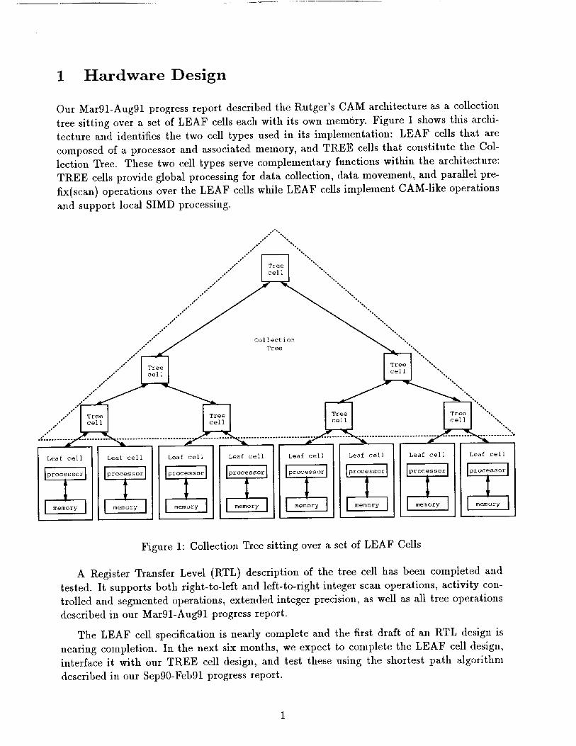
Our Mar91-Aug91 progress report described the Rutger's CAM architecture as a collection

tree sitting over a set of LEAF cells each with its own memory. Figure 1 shows this archi-

tecture and identifies the two cell types used in its implementation: LEAF cells that are

composed of a processor and associated memory, and TREE cells that constitute the Col-

lection Tree. These two cell types serve complementary functions within the architecture:

TREE cells provide global processing for data collection, data movement, and parallel pre-

fix(scan) operations over the LEAF cells while LEAF cells implement CAM-like operations

and support local SIMD processing.

°

_°°°°" *%%

°o* %%°

o/ ,%

Leaf cell Leaf cell Leaf cell Leaf cell Leaf cell Leaf cell Leaf cell Leaf cell

Figure 1: Collection Tree sitting over a set of LEAF Cells

A Register Transfer Level (RTL) description of the tree cell has been completed and

tested. It supports both right-to-left and left-to-right integer scan operations_ activity con-

trolled and segmented operations, extended integer precision, as well as all tree operations

described in our Mar91-Aug91 progress report.

The LEAF cell specification is nearly complete and the first draft of an RTL design is

nearing completion. In the next six months, we expect to complete the LEAF cell design,

interface it with our TREE cell design, and test these using the shortest path algorithm

described in our Sepg0-Feb91 progress report.

1.1 LEAF Cell Specification

Each LEAF cell is responsible for performing CAM-like operations and is composed of a

main processor connected to three support processors via multi-ported interface registers.

These support processors are the tree processor, memory processor, and IO processor (not

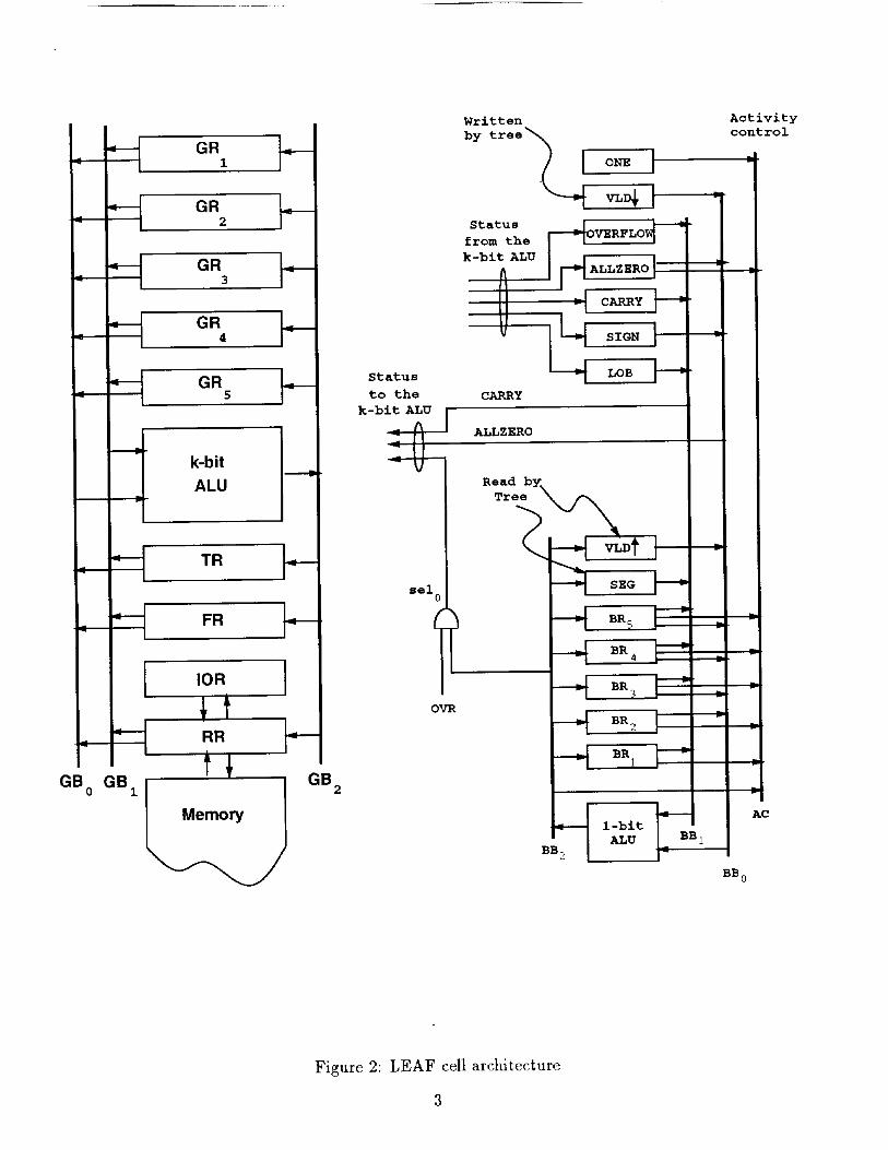
shown in Figure 1). The LEAF cell's main processor is composed of two communicating

components; a k-bit processor 1 for standard operations and a 1-bit processor used to control

activity within a LEAF cell. Figure 2 shows the interconneetion of these components.

1.2 Component Descriptions

The k-bit processor is a three bus (i.e., GB0, GB1, GB2) architecture composed of:

• a k-bit ALU

• five general purpose k-bit registers GR1, GR2, GR3, GR4, and GR5

• a dual ported k-bit flag register(FR) directly coupled to the fourteen 1-bit registers

* a dual ported (k+l)-bit tree register(TR) that provides the interface between leaf and

tree processor

• a tri-ported k-bit refresh register register(RR) that provides the interface between the

leaf, memory, and IO processors.

• a dual ported IO register(IOR) that provides the interface between the IO processor

and the refresh register (RR).

The 1-bit processor is a four bus (i.e., BB0, BB1, BB2, AC) architecture composed of:

• a 1-bit ALU

• five general purpose 1-bit registers BR1, BR2, BRa, BR4, and BRs

• a dual ported 1-bit segment register(SEG), read by the tree processor, that indicates

if a leaf processor is (SEG=I) or is not (SEG=0) the first element in a new segment.

• a dual ported 1-bit status register(VLDT), read by the tree processor, that indicates

if the tree processor should use (VLDT=I) or ignore (VLDT=0) the data in the tree

register.

• five 1-bit status registers(OVERFLOW, ALLZERO, CARRY, SIGN, LOB) that con-

tain the status of the k-bit ALU

1We expect the k-bit processor and its associated registers to be 32-bits wide; however, our design is not

restricted to 32-bit widths but parameterized as a function of word width.

" I 1

[I LStatus

to the

k-bi_

sel0

_VR

Written

by tree_ ONEvL_ Ii

Status [

from the _

cARRy

ALLZERO

Read by.

Tree \

Activity

control

I

AC

BB 0

Figure 2: LEAF cell architecture

3

• a dual ported 1-bit status register(VLDJ_), written by the tree processor, that indicates

if the leaf processor should use (VLD+=I) or ignore (VLD+=0) the data in the tree

register

• a 1-bit constant (ONE) used to activate LEAF cells

1.3 Interfaces between the 1-bit and k-bit components

The 1-bit and k-bit components communicate through the processor status registers (i.e., the

five 1-bit registers that maintain the status of the k-bit processor), through activity control,

and through dedicated connections joining the fourteen 1-bit registers and the low-order 14

bits of k-bit register FR.

Activity control is determined by the value carried on AC in the 1-bit processor and is

used to enable or disable the writing of both 1-bit and k-bit registers from their respective

output buses (i.e., GB_ and BB2). The value placed on AC can be obtained from the output

of the the 1-bit ALU (BB2) or from one of the 1-bit registers BR1, BR2, BRa, BR4, BRs,

ALLZERO, or ONE.

The dedicated connections between the 1-bit registers and the low-order 14 bits of FR

provides an additional interface that increases the bandwidth between the 1-bit and k-bit

components. These connections are used by the following operations.

• copy all 1-bit registers into FRo through FR13

• copy FR[0:4] into BR1 through BRs

• copy FR_ and FRo into SEG and VLDT,respectively

1.4 Instruction Fields

Operation of the LEAF cells is specified by the fields summarized in Figure 3. The estimated

width of each field is shown in parentheses. These specifications are tentative; refinements to

field size and instructions will be made as algorithms are implemented on tiffs architecture.

GOP

G0P encodes the operation to be performed by the k-bit ALU. The exact set of operations

has not been determined but includes AND, OR, XOR, addition, and subtraction as well as

sel-argl, sel-arg2. These last two instructions select the indicated input argument and route

it to the output.

RGB0 and RGBI

RGBo and RCB_ encode the refresh register, one of the k-bit general registers, the tree register,

or the flag register. Our initial design using 5 general registers is encoded as follows:

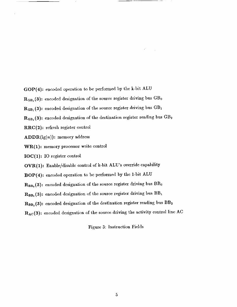
GOP(4): encoded operation to be performed by the k-bit ALU

RGB0 (3): encoded designation of the source register driving bus GBo

RGB_ (3): encoded designation of the source register driving bus GB1

l_aB2 (3): encoded designation of the destination register reading bus GB2

RRC(2): refresh register control

ADDR(Ig(n)): memory address

WR(X): memory processor write control

IOC(1): I0 register control

OVR(1): Enable/disable control of k-bit ALU's override capabihty

BOP(4): encoded operation to be performed by the 1-bit ALU

Rss0 (3): encoded designation of the source register driving bus BB0

RBB, (3): encoded designation of the source register driving bus BB1

RBB, (3): encoded designation of the destination register reading bus BB2

RAc (3): encoded designation of the source driving the activity control line AC

Figure 3: Instruction Fields

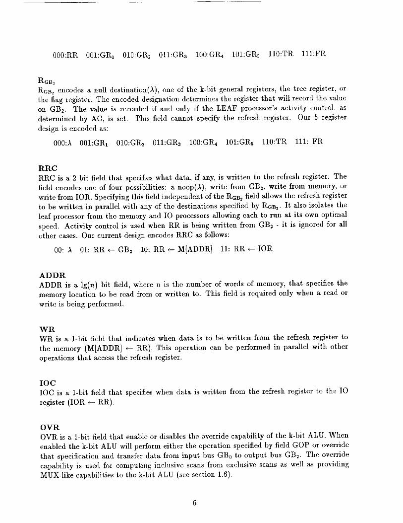
000:RR 001:GR1 010:GR2 011:GR3 100:GR4 101:GR5 ll0:TR lll:FR

RGB_

RGB2 encodes a null destination(A), one of the k-bit general registers, the tree register, or

the flag register. The encoded designation determines the register that will record the value

on GB2. The value is recorded if and only if the LEAF processor's activity control, as

determined by AC, is set. This field cannot specify the refresh register. Our 5 register

design is encoded as:

000:A 001:GR1 010:GR2 011:GR3 100:GR4 101:GRs ll0:TR 111: FR

RRC

RRC is a 2 bit field that specifies what data, if any, is written to the refresh register. The

field encodes one of four possibilities: a hoop(A), write from GB2, write from memory, or

write from IOR. Specifying this field independent of the RGB2 field allows the refresh register

to be written in parallel with any of the destinations specified by RGB2. It also isolates the

leaf processor from the memory and IO processors allowing each to run at its own optimal

speed. Activity control is used when RR is being written from GB2 - it is ignored for all

other cases. Our current design encodes RRC as follows:

00: ,_ 01: RR *-- GB_ 10: RR +-- M[ADDR] 11: RR _ IOR

ADDR

ADDR is a lg(n) bit field, where n is the number of words of memory, that specifies the

memory location to be read from or written to. This field is required only when a read or

write is being performed.

WR

WR is a 1-bit field that indicates when data is to be written from the refresh register to

the memory (M[ADDR] _-- RR). This operation can be performed in parallel with other

operations that access the refresh register.

IOC

IOC is a 1-bit field that specifies when data is written from the refresh register to the IO

register (IOR _-- RR).

OVR

OVR is a 1-bit field that enable or disables the override capability of the k-bit ALU. When

enabled the k-bit ALU will perform either the operation specified by field GOP or override

that specification and transfer data from input bus GB0 to output bus GB2. The override

capability is used for computing inclusive scans from exclusive scans as well as providing

MUX-like capabilities to the k-bit ALU (see section 1.6).

BOPBOP encodesthe operation to be performed by the 1-bit ALU. The bits are tile entries inthe truth table of the booleanfunction being computed.

RBB0,RBBI, and RatRBB0,RBB_,and RACeachencode8 registers (not the same registers). These encodings are

based on the interrelations between the 1-bit registers and a typical instruction mix. The

specific registers connected to each bus and their encodings will be altered as experience is

gained with algorithms on this architecture. The following are design goals which influence

these choices as well as an initial assignment of registers to busses.

Extended precision requires that the CARRY and ALLZERO status outputs from

the k-bit processor be fed back into the processor's CARRY and ALLZERO inputs.

Consequently, data paths that allow parallel routing of the CARRY and ALLZERO

registers to the k-bit processor must be supported.

Inclusive scans are completed in the LEAF processors using the results of the exclusive

scan produced by the tree and two additional steps 2 performed by the LEAF processor.

These steps makes use of the 1-bit ALU as well as the override feature of the k-bit

ALU and require that 1-bit registers VLD_ and SEG be presented in parallel to the

1-bit ALU. Details of these operations are described in section 1.6.

• RBB0 encodes one of BRA, BR3, BR4, BRs, VLDT, SIGN, ALLZERO, and VLDI

• field RBB, encodes one ofBR1, BR3, BR4, BRs, SEG, LOB, CARRY, and OVERFLOW

• The field RAC encodes one of BBA(i.e., the output bus of the 1-bit ALU) BR1, BRA,

BR3, BR4, BR_, ALLZERO, and ONE

RBB2

RBB2 encodes one of null(A), BR1, BRA, BR3, BR4, BRs, SEG, VLDT. This field determines

the register that will record the value on BB2. This value is recorded if and only if the

processor's activity control, as determined by AC, is set. Our initial design is encoded as:

000:A 001:BR1 010:BR2 011:BR3 100:BR4 101:BRs ll0:SEG lll:VLDT

1.5 Interaction between the LEAF and memory processors

The read and write commands form the conceptual interface between the LEAF processor

and the memory processor. They are executed by the memory processor and cause data to

be transferred between RR and the memory. These commands are encoded in two fields,

RI_C and WR. The read command is encoded in the RRC field as a command to move

data from memory to the refresh register. This command causes the memory processor to

2plus scans only require one additional step.

transfer the data at the location specifiedby ADDR to the refresh register. If tile read is

destructive, as is the case with a DRAM implementation, tile main control unit will issue a

write command to rewrite the contents of RR back to nmmory.

The write command specified by WR indicates that data is to be written from RR to

memory and must not conflict with RRC - the WR bit CANNOT specify write-to-memory

when RRC specifies read-from-nmmory. These commands are not affected by the processor's

activity control.

Once initiated by either a read or write the memory processor performs the data transfer

asynchronously. The LEAF processor should not change RR while tile menmry processor is

busy and is thus limited to using RR only when tile memory processor is idle.

1.6 Interaction between TREE and LEAF processors

Most of the interactions between the TREE and LEAF processor are of the standard variety;

however, there are two types of interactions that require special attention. One is the

handling of overflow between these two processors. The other is the communication of

scan results between the two processors.

These interactions are handled through the interface provided by TR, VLDT, SEG, and

VLDJ.. TR acts as a bidirectional data port connecting the two processors. When the tree

accepts data from the leaves it reads VLDI" and SEG. VLD T indicates if the data in TR

should, or should not, participate in the tree operation while SEG indicates if the leaf is, or

is not, the first in a segment. These two 1-bit registers can be read and written by the 1-bit

ALU; however, they may only be read by the tree.

When the tree provides data to the leaves it use VLD_ to indicates if the data in TR

should, or should not, be used by the leaf. VLDI can only be read by the LEAF processor

and can only be written by the TREE processor. There is dedicated hardware in the tree that

computes VLD_ as a function of the SEG, VLD_, and the direction of the scan (left-to-right

or right-to-left). Changing any of these three fields will cause VLDJ. to change.

1.6.1 Overflow Interactions

Since the TREE and LEAF processors jointly participate in numerical computations, the

LEAF processor must be responsive to overflow information generated by the TREE pro-

cessor. This information is stored in a single bit in TR and must be used by the LEAF

processor's k-bit ALU to determine its overflow condition. The overflow condition of a LEAF

cell operation (even data movement such as GRI +-- TR) that involves the tree register as a

source must be dependent on the overflow condition generated in the tree. If TR indicates

an overflow from the tree, the LEAF processor must complete the specified operation and

set the overflow status to true. The overflow status must also be set if the LEAF processor

performs an arithmetic operation that itself generates an overflow.

In the case when the tree is not supplying data to the leaf (i.e., VLD.L is 0), the overflow

field in TR is ignored.

1.6.2 Inclusive and Exclusive Scans

When an inclusive scan is desired, tile LEAF processor must compute it from the TREE

cells exclusive scan and its own internal data.

These operation are performed using the override capability of the k-bit ALU which

permits the ALU to either execute the operation specified or to ignore the operation and

replace it with a data transfer. The data transfer routes the data on input bus GB0 directly

to output bus GB2. When an override is in effect the operation specified by GOP and the

data on input bus GB1 are ignored by the k-bit ALU.

Figure 4 shows a operation and its overridden counterpart. Notice that the data transfer

that replaces the specified operations ignores the fields RGBI and GOP but uses the fields

RGBo and RGB2 without alteration.

Operation

Overridden Counterpart

Operation Mnemonic

GP_ e-- (GRj op GR_)

GI_ _ GRj

Operation field specification

RaB0=j, RcB,=GRk, Rcs2=i, GOP=op

RCBo =j, ROB= =i

Figure 4: Comparison of normal operation and it overridden counterpart

In order to produce inclusive scans from exclusive sculls two cases must be considered.

One, when the tree processor provides data on which the inclusive scan depends (VLD+=I

A SEG=0) and two, when it does not (VLDJ.=0 V SEG=I). Notice that these conditions

are functions not only of the results produced in the tree but also of the segmentation bit in

the leaf processor. This latter dependence is due to the fact that the first leaf processor in

a segment (SEG=I) must ignore the data it receives from the tree since this data is from a

different segment. The LEAF processor must be able to distinguish between these cases and

complete the inclusive scan appropriately. Figure 5 shows the operations required of the the

LEAF processor for these two cases.

Tree data should be used GP< *- (GRj op TR)

Tree data should be ignored GR; _ GRj

Figure 5: Leaf operations for forming inclusive scans from exclusive scans

Since the second of these operations is an overridden version of the first, the choice

between the two operations can be performed by the override capability of the k-bit ALU

by using the single instruction show in Figure 6.

OVR

on

k-bit operation

GP_ _- (GRj op TR)

1-bit operation

A _- (VALi A SEG)

Figure 6: Using OVR to form inclusive scans from exclusive scans

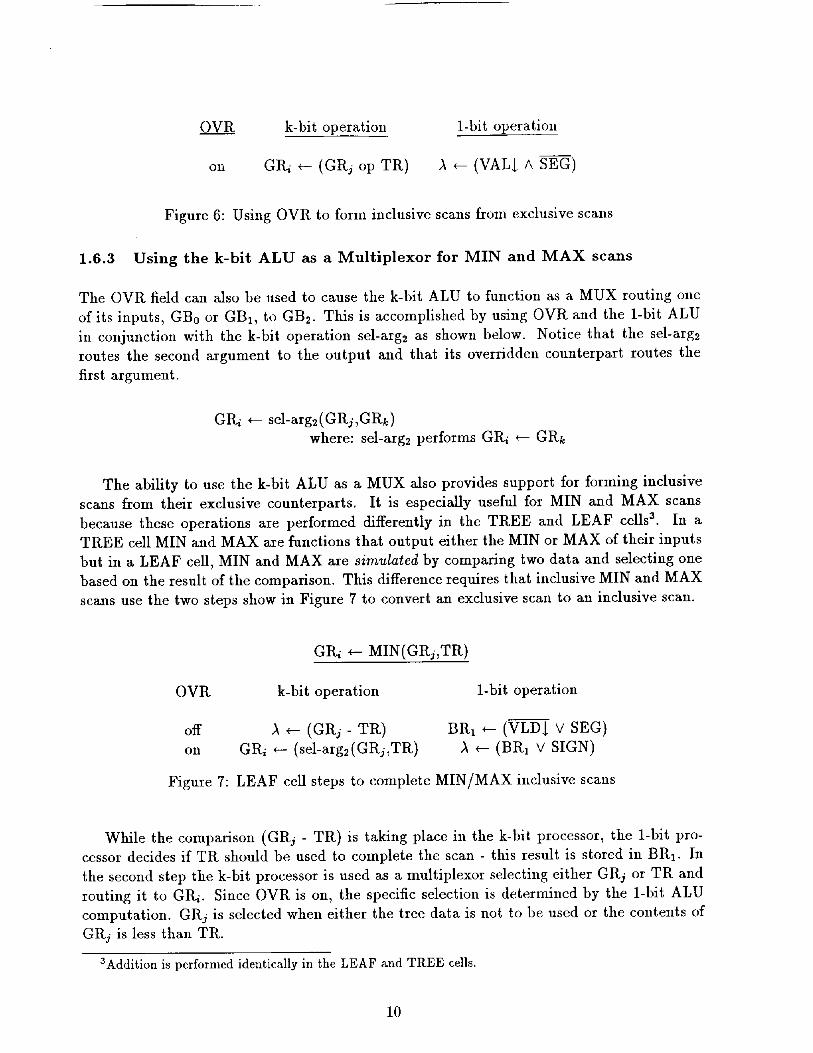
1.6.3 Using the k-bit ALU as a Multiplexor for MIN and MAX scans

The OVR field can also be used to cause the k-bit ALU to function as a MUX routing one

of its inputs, GB0 or GB1, to GB2. This is accomplished by using OVR and the 1-bit ALU

in conjunction with the k-bit operation sel-arg2 as shown below. Notice that the sel-arg2

routes the second argument to the output and that its overridden counterpart routes the

first argument.

GP_ _ sel-arg2(GR¢,GR_)

where: sel-arg2 performs GI_ _-- GRk

The ability to use the k-bit ALU as a MUX also provides support for forming inclusive

scans from their exclusive counterparts. It is especially useful for MIN and MAX scans

because these operations are performed differently in the TREE and LEAF cells 3. In a

TREE cell MIN and MAX are functions that output either the MIN or MAX of their inputs

but in a LEAF cell, MIN and MAX are simulated by comparing two data and selecting one

based on the result of the comparison. This difference requires that inclusive MIN and MAX

scans use the two steps show in Figure 7 to convert an exclusive scan to an inclusive scan.

OVR

off

on

GP_ *- MIN(GRj,TR)

k-bit operation

A e-- (GRj- TR)

GI_ _- (sel-arg2 (GRj,TR)

1-bit operation

BRt _ (VLDI V SEG)

A e-- (BR1 V SIGN)

Figure 7: LEAF cell steps to complete MIN/MAX inclusive scans

While the comparison (GR:/ - TR) is taking place in the k-bit processor, the 1-bit pro-

cessor decides if TR should be used to complete the scan - this result is stored in BR1. In

the second step the k-bit processor is used as a multiplexor selecting either GRj or TR and

routing it to GI_. Since OVR is on, the specific selection is determined by the 1-bit ALU

computation. GRj is selected when either the tree data is not to be used or the contents of

GRj is less than TR.

ZAddition is performed identically in the LEAF and TREE cells.

10

1.6.4 Inserting identity elements

TREE cells perform exclusive scans (i.e. the initial element in a segment is tile identity

element for the operation) but do not insert the identity element into the result. In order

for the result to contain the identity element the LEAF processor must insert it.

This is accomplished using the MUX-like capabilities of the LEAF processor to choose

between the data provided by the tree and the identity element for the operation. Figure 8

shows the constants that are expected to be of special interest. These five constants can be

constructed from a 3-bit field in which one bit specifies the high order bit, one the low order

bit, and one the internal bits.

Constant Use

0 00..00 0

1 11..11 1

1 00..00 0

0 11..11 1

0 00..00 1

identity for +, OR, MAX on positive integers

identity for AND, MIN on positive integers ; decrement

identity for MAX on 2's complement

identity for MIN on 2's complement

increment

Figure 8: Important Constants

1.7 Activity control

Activity control is used on all k-bit and 1-bit registers. These registers latch their input

values at the end of each execute cycle if and only if they are selected by RcB_ or RBB=

and AC is set. There is no activity controlled write-to-memory; however, the effect of this

operation can be obtained by using the standard memory operations in conjunction with an

activity controlled operation on RR. Figure 9 shows how this is accomplished.

M[ADDR] _- GI_ in all active leaf nodes

RR _ M[ADDR]

RR e-- GR/

M[ADDR] +-- RR

mediated by AC

Figure 9: Activity Controlled write to memory

11

March 92

CIRCUIT DESIGN TOOLUSER'S MANUAL*

Keith M. Miyake and Donald E. Smith

LCSR-TR-181

Laboratory for Computer Science ResearchHill Center for the Mathematical Science

Busch Campus_ Rutgers University

New Brunswick, New Jersey 08903

*This work was supported by the Defense Advanced Research Projects Agency

and the National Aeronautics and Space Administration under NASA-Ames

Research Center grant NAG 2-668.

Contents

1 Introduction 1

1.1 Circuit Definition ................................. 2

1.2 Model Creation .................................. 2

2 The Definition Language 4

2.1 Syntax Conventions ................................ 4

2.2 Variables and Assignment ............................ 5

2.3 Expressions .................................... 6

2.4 Naming Conventions ............................... 7

2.5 Cable Definitions ................................. 9

2.6 Module Definitions ................................ 11

3 Command Syntax 19

3.1 Filenames ..................................... 19

3.2 Current Generated Module ............................ 19

3.3 Current Submodule ................................ 20

3.4 Parent Constructor ................................ 20

3.5 Command Naming ................................ 20

3.6 Design Tool Commands ............................. 22

4 Implementation Details 28

4.1 Primitive Modules ................................ 28

4.2 Simulation Construction ............................. 28

4.3 Bus Signals .................................... 29

4.4 Simulation Events ................................. 29

4.5 Simulation Runs ................................. 29

5 Startup Options 31

5.1 Command-line Arguments ............................ 31

5.2 simrc File ..................................... 32

A The Lexer

B Primitive Modules

C Module Examples

D Error Messages

34

37

42

46

ii

Chapter 1

Introduction

The design of the CAM ctfip has been done in a UNIX software enviromnent using a design

tool that supports the definition of digital electronic modules, the composition of these mod-

ules into higher level circuits, and event-driven simulation of these circuits. Our tool provides

an interface whose goals include straightforward but flexible primitive module definition and

circuit composition, efficient simulation, and a debugging environment that facilitates designverification and alteration.

The tool provides a set of primitive modules which can be composed into higher level

circuits. Each module is a C-language subroutine that uses a set of interface protocols

understood by the design tool. Primitives can be altered simply by rccoding their C-code

image; in addition new primitives can be added allowing higher level circuits to be described

in C-code rather than as a composition of prinfitive modules - this feature can greatly enhance

the speed of simulation 1.

Effective composition of primitive modules into higher level circuits is essential to our

design task. Not only are the standard features of a description language required but in

addition, features such as recnrsive descriptions of circuit composition, parameterized module

descriptions, and strongly-typed port types are essential to efficient circuit design. These

features are supported by our design tool's composition language which allows the user to

specify a hardware description in a C-like syntax. Parameterized modules, recursive and

iterative descriptions, macro-like capabihty to describe collections of wires (i.e., cables), and

decision ma,king support that allows context sensitive module expansion are provided by

our tool. In addition, our tool can determine the cost of a circuit based on the costs of its

primitive modules. This feature is not exact but does provide a good approximation of the

complexity of the designed circuit.

Simulation is performed by an event-driven simulator that handles gates as well as tri-

state bi-directional busses and provides the user not only with a view of what a circuit is

computing but also control over the circuit so that design, flaws can be effectively isolated

1Converting a higher-level circuit into a primitive module is straightforward when the timing of theprimitive module need not be identical to the higher level circuit. Higher level circuits can be converted toprimitive modules with identical time performance; however, the conversion process is much more complex.

and corrected. The simulator is controlled with a command language which allows tile user

to see a wire or set of wires, as well as change the values on wires. Operations can be done

immediately (i.e., at the time the user enters them) or scheduled to take place at a specified

time. Simulations can be run for a specific period of time or until a certain condition is

detected in the hardware. They can be controlled from the keyboard or indirectly from a

file.

Tile design tool consists of two main parts: the command and definition languages. The

definition language is used to read circuit definitions. The command language controls the

actions of the simulator. These topics are detailed in sections 2.5 and 2.6.

Following is a brief introduction on the definition and creation of circuit models. It

defines many terms used later.

1.1 Circuit Definition

The circuit definition language describes connections between primitive objects. These ob-

jects, called primitive modules, have functionality predefined in the design tool. Primitive

modules have a special set of entry points which are connected when forming the circuit

model. These entry points are called ports and the connections between them are referred to

as siguals or wires. There is a causality between connected modules. Execution of a module

may affect modules connected to it.

The design tool reads descriptions using a definition language. The language consists of

two types of object definitions: module and cable. Cable definitions group related signals

together. Module definitions specify primitive modules and their connections. A module may

define other modules as children of itself, and specify connections between its child modules.

In this case the module is referred to as a composite module.

The circuit is built from a set of hierarchical module and cable definitions. Flattening

the hierarchy produces the basic model of a set of primitive modules connected by wires.

In order to name objects in the hierarchical design, hierarchical names are used by the

design tool. These names specify objects which cannot be directly referenced within the

current context. This is done by supplying a list of names specifying a path to the object.

Each field in the composite name is separated by the dot character '.'.

1.2 Model Creation

The creation of a circuit model is performed in phases.

When a cable or module defiuition is read, its syntax is checked and the definition is stored

as a master definition. These definitions may have input argmnents which need assignment.

When a module is created, input arguments to master definitions are assigned resulting in

a new definition type. These definitions, which have specific input arguments, are referred to

as definition instances. Each definition instance is fully examined, checking the consistency

of the connections m_de and the referenced modules.

The circuit model is made front these definition instances. Tile model is designed for

speed iu simulating the functionality of the circuit and contains all structures necessary for

simulation. Such a model is called a generated module or simulation instance.

Chapter 2

The Definition Language

The definition language is used to describe digital electronic circuits by building lfierarchical

structures connecting primitive modules. A definition file consists of a sequence of module

and cable definitions. Modules come in two types: primitive and composite.

Primitive modules are the basic building blocks of the definition language. These objects

perform operations defined by C functions which have been preeompiled into the design tool.

A list of primitive modules is given in appendix B.

A composite module definition defines submodules of itself and connections to be made

among their ports, as well as its own ports. Attaching submodule ports causes interactions

between the operations of the respective modules.

Cable definitions allow signals to be identified in groups, which simplifies connection of

ports.

Module and cable definitions are similar in structure and are analogous to functions in

a conventional programming language. They may have formal input argmnents and may

use other definitions (as well as their own) recursively. Termination of such recursion is not

assured.

2.1 Syntax Conventions

The language syntax descriptions used in this manual is a variant of the Backus-Naur form.

Following is a list of syntax rules:

1. Boldface type denotes reserved words.

2. Lowercase words, which may have embedded underscores, denote syntactic constructs.

3. Character tokens are shown using typewriter type. Most punctuation characters are

used as character tokens, with exceptions stated below. Note that the exceptions are

printed in Roman type.

4. The vertical bar '1' separates alternate syntax items when it is used at the beginning

of a line.

5. Square brackets ('[', ']') enclose optional items.

6. The dollar sign '$' in a syntax rule denotes the remainder of the line as a conlment.

'$' is not used in the syntax.

2.2 Variables and Assignment

A variable is a name associated with an integer value in a module or cable definition. Vari-

ables have no meaning outside the current definition. A variable name may be any valid

string token (quoted or unquoted; see appendix A). There are no arrays of variables. A

variable may have the same name as signals, modules, or cables since its context is distinct.

There are three variable types: input, loop, and assignment. Within a specific definition, a

variable may be used as only one type.

Input Variables

Input variables are arguments to a module or cable defilfition. They are determined at

invocation and may not be reassigned within the current object. These variables are valid

throughout the current object. Each input variable of a defilfition must be given a value

upon use.

Loop Variables

Loop variables are used in for loops in the component section of modules. Each for loop

controls the assigmnent of a single loop variable. Loop variables are only valid within the

controlling loop, and may not be reassigned within the loop.

Assignment Variables

Assigmnent variables are used in the component section of modules. They are set using the

assign statement ( string_token <- arith_expr ; ). This assigns the current value of the

expression to the variable. Once a variable has been assigned to, it is valid until the end

of the module. Each subsequent use of the variable gets the assignment value unless the

variable has been reassigned. Assignment variables may not be reused as loop variables.

Control flow variations resulting from if statements or loops may allow an assignment

variable to be referenced prior to assignment.

Cables only have input variables since they have no component section.

2.3 Expressions

Expressions are used in various ways to control the assembly of modules. There are two types

of expressions: arithmetic and logical. Arithmetic expressions result in integer values. Logical

expressions return one of the values TRUE or FALSE. Arithmetic and logical expressions

are not interchangeable.

Arithmetic Expressions

Arithmetic expressions compute integer values. They may be string tokens (variables),

numeric tokens (constants), or may be created by application of an arithmetic operator

to one or more arithmetic expressions.

arith_expr :=

string_token

numeric_token

- arith_expr

( arith_expr )

arith_expr * arith_expr

arith_expr / arith_expr

arith_expr _, arith._expr

arith_expr + arith._expr

$ variable value

$ constant value

$ arithmetic negation

$ arithmetic grouping

$ multiphcation

$ division

$ modulus

$ addition

arith_expr - arith..expr $ subtraction

Division operations return a truncated result (using C convention), since integer division

is not exact.

There are three levels of arithmetic operator precedence. Unary operators (negation and

grouping) share the highest precedence. Multiplication, division, and modulus (*,/, Z) have

equal precedence, below that of the unary operators. Addition and subtraction (+, -) share

the lowest precedence.

All binary arithmetic operators associate left-to-right.

Logical Expressions

Logical expressions compute the value TRUE or FALSE. They are constructed by the use

of relational or logical operators. Relational operators produce a logical expression based on

the validity of a relational query between two arithmetic expressions. Logical operators use

one or two logical expressions to produce a single logical expression. There are no logical

variables or constants.

log_expr:--arith_expr > arith_expr $ greater than

I arith_expr >= arith_expr $ greater than or equal to

I arith_expr < arith_expr $ less than

I arith_expr <= arith_expr $ less than or equal to

[ arith_expr = arith_expr $ equal to

I arith_expr ! arith_expr $ not equal to

I ~ log_expr $ logical negation

] ( log_expr } $ logical grouping

I log_expr _: log_expr $ logical AND

I log_expr I log_expr $ logical OR

Note that the vertical bar in the logical OR represents the character '1 '.

Tile use of arithmetic expressions as operands eliminates precedence or assoeiativity with

regard to relational operators.

There are three levels of logical operator precedence. Unary logical operators (negation

and grouping) have the highest precedence, followed by logical AND. Logical OR has the

lowest precedence of logical operators.

Logical grouping syntax is distinct from that of arithmetic grouping. This reinforces the

idea of noneompatibility between expression types.

2.4 Naming Conventions

Each child object (signal, cable, or submodule) in a definition must be given a unique name.

This allows unambiguous signal naming within simulation instances (for design verification).

Names of child objects must be string tokens (quoted or unquoted).

An object name may have a single associated array index. This index is specified by

an arithmetic expression enclosed in square brackets following the name. The string token,

excluding the array index, is called the root name of the object.

objeet.alame :=

string_token

] string_token [ arith_expr ]

Note that the square brackets do not represent optional arguments.

Example:

The root name of an object "a[5]" is simply "a".

It is often useful to name lists of objects. In this case, a modified array notation, called

an object list, may be used to specify a range of array indices. This is done by supplying

a start and end index for the array, separated by a colon ' :'. The notation is equivalent to

supplying each object name in order, beginning with the start index, and iterating until the

end index is reached. If the start index is less than the end index iteration increments by

one, otherwise it decrements by one.

objeetdist :=

string_token [ arith_expr : arith_expr ]

Note that tile square brackets do not represent optional arguments.

Example:

"a[1:2]" expands to "a[1]" "a[2]".

"a[2:1]" expands to "a[2]" "a[1)".

A list of objects may contain single object names and object lists.

object.name.list :=

object._lame

[ objectAist

[ object.Ilame object_namedist

I objectAist object_.uameAist

In a module definition, each internal subcomponent or signal must have a distinct name

(root name and index). Also, objects with the same root name must have similar types.

This means that signals, components and cables may not share root names. Furthermore,

components or cables which share a root name must share the same master definition. These

checks are performed during tile creation of module definition instances.

It is often necessary to name an object which cannot be directly referenced from the

current level. In this case a composite name is used, using the dot character '.' to separate

levels. This is referred to as a hierarchical name.

hierarchical._lame :=

object_Ilame

I object_name . hierarchical_name

Example:

The hierarchical name "a.b" refers to an object "b" wtfich is a child of object

"a", where "a" is a child of the current module.

Hierarchical naming may be used with array expansion, in wtfich case rightmost indices

are expanded first.

hierarchicalAist :=

object_name

[ objectAist

I object_name . hierarchical_list

[ objectAist . hierarchicalAist

Example:

"a[l:2].b[3:4]" expands to "a[1].b[3l" "a[1].b[4]" "a[X].b[3]" %[2].b[4]'.

The hierarchical analog to an object name list, called a hierarchical list, may now bedefined. Note that everyhierarchical nameis alsoa hierarchicallist.

hierarcllicalatamelis t :=hierarchical_listI hierarchical_listhierarchical_name_list

2.5 Cable Definitions

A cable represents an ordered list of signals, each signal having all associated type. Signal

typing is used to ensure that the use of a module is consistent with its definition.

cable_definition :=

cable string_token [ ( variableAist ) ] typed_signalAist end

variableAist :=

string_token

I string_token , variableAist

typed_signalAist :=

signal_nameAist signal_type

[ signalnameAist signal_type typed_signalAist

signal_nameAist :=

object-I*ameAist

[cable_use

[ object_nameJist signal_ammeJist

I cable_use signal_namelist

signal_type :=

input

[output

[ inout

The string token following cable is the cable name. This name is used for future refer-

ences to the cable. The variable list is a list of input variables for the cable. When the cable

is used, each input variable must be given a value. The typed signal list is a list of the wires

which comprise the cable. It may include cables uses, which is defined below. Each signal

is given one of three allowable types: input, output, or inout. The meaning of the types

will be described in section 2.6.

Example:

cable cl

sl s2 input

s3 output

s4 inout

end

In the example, signals "sl" and "s2" are both input.

After a cable has been defined, it may be used anywhere that a signal may be used. This

includes being used in other cable definitions. The following syntax defines a name as a useof a cable.

cable_use :=

cable string_token [ ( argument_list ) ] object_name

] cable string_token [ ( argument_list ) ] { objectatamelist }

argument_list :=

arith_expr

I arith_expr , argument_list

The string token following cable is the name of a cable definition. The argument list

given must be exactly the same size as the number of input variables to the cable definition.

Following the arguments is the list of new cable instance names.

Example:

cable cl cil

cable cl { ci2 ci3 }

The first use defines a single instance "cil" of cable "cl". The second use defines

two additional instances, "ci2" and "ci3", of cable "cl".

When a cable is used in another cable definition, the type of the resultant signal depends

on both the signal type given in the previous definition, and the type given to the cable use.

The following matrix shows tim retyping rules:cable _ype subsignal type

input output inout

input

outputinout

input output inout

output input inout

inout inout inout

After a cable instance has been defined, each use of the instance name represents the

list of its component signals in order. Each signal name in the list is a tfierarchical name

consisting of the cable instance name and the component signal name. Individual signals

within the cable may be accessed by naming the signals hierarchically.

Example:

cable c2

sl input

s2 output

end

i0

cable c3

cable c2 scl input

cable c2 sc2 output

cable c2 se3 inout

end

In cable "c3", signal "scl.sl" would be input and "scl.s2" would be output.

Because of retyping, signal "sc2.sl" would be output while "sc2.s2" would be

input. Both subsignals of "sc3" would be inout.

Example:

If we make a instance "ci4" of the cable type "cl", individual signals may be

referenced as "ci4.sl", "ci4.s2", "ci4.s3", and "ei4.s4". This set of signals, in

order, cau be referenced simply as "ci4".

Cable definitions may use other cable definitions, including those wlfich are not yet

defined (forward referencing). There is no check for recursive cable references, which do not

terminate.

2.6 Module Definitions

Two types of modules (primitive and composite) are used in circuit designs. Primitive mod-

ules are objects with predefined functions. Composite nlodules define connections between

primitive and composite modules.

module_definition :=

module string_token [ ( variable_list ) ] [ cost_section ]

[ port_section ] [ signal_section ] [ component_section ] end

The string token following module is the module name. This name is used to reference

the module in future use. As with cable definitions, when a module is used each input

variable must be given a value.

Additional module examples are given in appendix C.

Cost section

The cost section is used to estimate the relative expense of building modules using several

technologies. Each module definition instance has associated cost values. These costs may

be explicitly defined in the cost section, or may be implicitly defined as the sums of the

costs of its submodules. Primitive modules should define explicit costs with a cost section.

11

Composite modules should include a cost section if the hardware implementation of the

module does not correspond to tile functional model represented by its subcomponents.

cost_section :=

costs cost_pairJist

cost_pairAist :=

cost_pair

[ cost_pair cost_pairAist

cost_pair :=

nmos : arith_expr

[cmos : arith_expr

t gateInput : arith_expr

Currently there are three cost criteria: nmos, cmos, and gateInput. If a technology

cost is given more than once, the last cost pair is used.

Example:

module ml(vl)

costs

nmos: 2*vl

cmos: 10

gateInput: 20

end

Port section

The port section is an ordered list of the external connections of the current module. Ports

are special signals which are used to connect to the module in later uses. A module with no

ports cannot be referenced by another module. The order of port signals is important and

determines proper connection of the module.

port_section :=

ports typed_signalAist

The typed signal list is the same as used in cable definitions, with the same subsignal

retyping rules.

Type information defines the proper use of the signal in the module and what connections

are allowed if the module is referenced by a composite module.

input implies that the signal is generated from an external source.

output implies that the signal is generated within the current module.

inout does not state the source of the signal. It causes the signal to be a

(bi-directional) bus, which nmst be driven by tri-state drivers.

12

Tile following rulesgovernvalid connectionsto eachtype of port signalwithin the currentlnodule:

input: No output signalnlay be connectedto tile signal. At leastoneprimitive descendentmodulenmst usethe signalasan input.

output: At leastone primitive descendentmodule must usethe signalas anoutput.

inout: At leastoneprimitive descendentlnodulemust usethe signalasall input or output.Additionally, everyconnectedoutput must be a a tri-state driver (the signalis a bus).

Missing or inconsistently typed signal connections are reported upon creation of module

definition instances.

Example:

module m2

ports

pl input

p2 output

p3 inout

end

Signal section

Tile signal section defines internal signMs of the current module. These internal signals nmst

be distinct from port signals and may not be referenced by other modules. Every signal used

in a module definition nmst be defined in either the port or signal section. The order in

which internal signals are defined is not important.

signal_section :=

signal signalJlame_list

Each signal defined in the signal section is given a special type of internal, If a cable

use is defined in this section, all resulting signals are also typed as internal.

The internal type means that the signal is both generated and used by priniitive de-

scendents of the current module.

Example:

module m3

signals

sl s2 s3

end

13

Component Section

The component section determines how composite module are built from other modules.

This is accomplished by 'executing' component statements ilt order, similar to conventional

programming languages. Primitive modules, whose functions are defined by C code, do not

use their component sections.

component_section :=

components component_st atement list

component_statement_list :=

component_statement

I component_strut component_statementlist

component_.statement :=submodule._statement

assign.statement

join_statement

error_statement

grouping..statement

if_statement

for_statement

while_statement

break_statement

$ declare a child module

$ assign a value to a variable

$ create a link between a group of signals

$ print an error message

$ group multiple statements

$ execute statements conditionally

$ execute a statement loop iteratively

$ execute a statement loop conditionally

$ exit from loops

Submodule Statement

Submodule declares a module as a child of the current module. It also designates attach-

ment of signals to tile ports of the child module.

submodule_statement :=

object_name string_token [ ( argument_list ) ] hierarchical_name_list ;

The initial object name is the local name given to the submodule. This name is used to

refer to the child module within the current ,nodule. Speeifially, it is used in hierarchical

naming. The next string token is the name of a module definition. The number of arguments

given must match the number of input variables of the module definition. Next is a list of

signals to be attached to the ports of the child module. Because every signal must be

declared in the port or signal section, references to cables use hierarchical names (and not

cable uses). Each signed in this list will be connected to the corresponding port of the

previously defined module in order. The signal list must be the same size as the number of

ports of the previously defined module. The port and connecting signal must conform, using

the rules stated under the port section.

Example:module m4

port s

14

m4i input

m4o output

signals

icl

end

module m5

ports

mSi input

m5o output

components

scl m4 m5i m5o;

end

In the example, module "1115" defines a child module of type "m4" and gives it

the local name "scl". The hierarchical name which refers to the signal "icl" in

"m4" is "m5.scl.icl". Note that the ports of "m4" and the connecting signals in

"mS" correspond in type.

Assign Statement

Assign associates an integer value with a variable. The target of assign may be any unused

variable name, or an assignment variable. Execution of assign causes the expression value

to be computed and assigned to the variable.

assign_statement :=

string_token <- arith_expr ;

The string token names the variable to be assigned.

Example:

module m6

components

vl <- 2;

v2 <- vl

vl <- i;

end

*2;

The first assign creates a new variable "vl" with a value of 2. The second creates

"v2" and uses "vl" to compute "v2" as 2*2 = 4. The final assign changes "vl"

to 1, but does not affect "v2".

Join Statement

Join merges a set of signals to form a single signal. After a join has been completed, any

15

member can be used to represent the set in other component statements (including joins).

Every signal used in a join must be declared in the port or signal section of the module.

The merging of signals caused by a join may introduce non-obvious incousistencies in

the connection of modules. These inconsistencies are reported upon execution of the join.

join_statement :=

join [ tfierarchicalatame-list ] ;

Note that the square brackets above do not indicate an optional argument.

Example:module m7

signals

sl s2 s3

component s

join [st s2];

join [s2 s3];

end

The first join merges signals %1" and "s2". The second merges the signal "s3"

with the signal which is the join of "sl" and "s2".

Error Statement

Error allows the user to print a message during the course of module generation. The

message is a single string (no variables), and is designed mainly for identifying situations

that should not occur.

error._statement :=

error string_token ;

Execution of error causes activation of an error message with the error flag mask acti-

vated. The error ntask value is given in appendix D. These messages nlay be suppressed or

may cause program termination by options in the simrc file.

Grouping Statement

Grouping a/lows multiple component statements to act as a single statement lexically. This

allows multiple statements to be used as targets in if, for and while statements. Grouping

has no affect in other contexts.

grouping._statement :=

{ component_statement-list }

Note that there is no semicolon following the grouping statement.

Grouping does not affect the lexical scope of any variable.

16

If Statement

If allowsconditionalexecutionof a statementdependingon the result of a logical expression.Multiple statementsmay be executedby tile useof grouping.

if_statement:=if log_exprcomponent_statenmnt[ else component..statenmnt] ;

If executes tlle first component statement when the logical expression is TRUE. When the

logical expression is FALSE, the second component statement (in the optional else clause)

is executed if available.

For Statement

For executes a statement a specified number of tinms. Multiple statements may be executed

by the use of grouping.

For evaluates two bounding expressions once to find the inclusive range for its loop

control varable. The target statement is then repeatedly executed with the loop variable

set to each value in the range. The loop variable is initially set to the value of the first

expression. If the first expression is less than the second expression, the loop variable is

incremented by one after each iteration; otherwise the variable is decremented by one.

The loop variable is not allowed to be a input or an assignment variable, and may not

be assigned within the loop. This guarantees termination of for.

for_statement :=

for string_token = arith_expr , arith_expr component_statement

While Statement

While executes a statement as long as a logical expression remains TRUE. Multiple state-

ments may be executed by the use of grouping.

While first evaluates the controlling logical expression. If it is TRUE, the target state-

ment is executed, and while is reexecuted. If it is FALSE, execution continues at the

statement immediately following the while.

Termination of while is not guaranteed. There is no check for non-termination.

while_statement :=

while log_expr component_statement

Break Statement

Break is used to halt processing of for and while statements. Break disregards pend-

ing statements in the current target component, and continues execution at the statement

17

immediately following tile current for or while statement.

Break takesan argumentwhich is the number of nestedloopsto break. A nonpositiveargumenthasno effect. If tile argument is larger than the numberof nestedloops,creationof the module is completedat tile break. Break doesnot affectparent modules.

break_statement:=break arith_expr ;

18

Chapter 3

Command Syntax

Tile command syntax controls what actions are taken. These commands control tile defini-

tion and execution of circuit models.

Commands are normally read from standard input. They may be directed from a file by

using an input flag or a command statement.

3.1 Filenames

A special syntax is accepted to facilitate the use of filenames. Filenames are allowed to

be string tokens separated by periods '. '. This allows specification of most local filenames

without having to use quoted strings.

file J_ame :=

string_token

I string_token . file_name

Quoted strings must be used in order to use the UNIX directory structure.

3.2 Current Generated Module

The name of the last generated module to be referenced is saved. This is known as the

current generated module. The current generated module is used when commands are issued

which omit the optional module name. The current generated module is automatically set

by generate_ and may be changed using set.

19

3.3 Current Submodule

Each generated module has a single current submodute. The current submodule is used as

a shorthand notation for a single submodule in each generated module. This allows simple

reference to the submodule during testing.

The current submodule is referenced by beginning a command name with character '_'.

The current sublnodnle of a simulation instance is initially tim top level module generated.

It may be changed using set.

3.4 Parent Constructor

The command naming syntax contains a parent constructor "'. As each field is read in the

left-to-right expansion of a hierarchical name, the partial name corresponds to an object in

the current module. When the parent constructor is read, the new object referenced by the

partial name is set to the parent of the current object.

The parent constructor is usually used in conjunction with the current submodule '¢'.

Use of the parent constructor '^' with an array of child modules may cause problems.

3.5 Command Naming

Names in the command syntax are similar to hierarchical names in definitions. There are

additional rules which apply to command names:

• The name of the current generated module or the current submodule identifier '¢' must

be the first field in the hierarchical name.

• There is a parent constructor '^' which changes the target to the parent of the current

target.

We now define an object name in the command syntax.

command_object :=

]string_token

[_ . command_object_tail

I string_token . command_object_tail

2O

command_object_tail :=

] object_name

1" . command_object_tail

] objectalame . command_objectXail

We also define a list of command objects defined by array expansion. This correspondsto the hierarchical list ill the definition syntax.

commandJist :=

I string_token

I¢ . commandAist_tail

]string_token . command_list_tail

command_list_tail :=

[ object_uame

I objectJist

]" . commandJist_tail

] object_name . commandlist_tail

[ object_list . command_list_tail

Finally, a general list of command names is defined. Note that every command object isalso a command list.

command_objectJist :=

command_hst

I commandJist command_object_list

21

3.6 Design Tool Commands

command_statement :=

source_statement

clear_statement

generate_statement

rum_statmnent

reset _statement

destroy_statement

read_statement

close_statement

pause_statement

assignment_statementshow_statement

showvector_statement

timed_statement

set_statement

repeat._statement

quit_statement

$ read in a definition file

$ dear all current definitions

$ generate a module for simulation

$ simulate a generated module

$ reset signals in a generated module

$ destroy a generated module

$ read commands from a file

$ close an open command file

$ transfer control

$ assign values to signals

$ display signal vectors

$ display signal vectors as a group

$ execute a command during simulation

$ set options

$ loop read a command file

$ exit the program

Source Statement

Source reads in a file of module definitions. The entire file is read using the stated definition

language rules. Modnle syntax is checked as the definition file is read. Definitions are checked

for consistency only when referenced by a generate.

source_statement :=

source file._name ;

If source causes a module to be redefined, the new definition will be used only in future

module definition instances. Previously defined instances will continue to use the previousdefinition.

Clear Statement

Clear deletes all definitions and simulation instances. This is equivalent to restarting the

design tool.

clear_statement :=

clear ;

Generate Statement

Generate creates a simulation instance of a module definition. The module should have been

22

previously read using a source. The simulation model is usedto test correctness of designs.

Generating a module causes all consistency checks on submodule use to be tmrformed. The

consistency rules have been stated along with tile definition syntax.

Each generated module is set to a special initial state in which all signals have an unde-fined value.

Gereration of a module causes it to become the current generated module.

generate_statement :=

generate string_token [ ( argumentlist ) ] ;

The string token specifies the module to be generated. The arguments given nmst match

the number of input variables of the module.

Run Statement

Run executes a simulation run of a generated module. Events queued for the module are

evaluated until all events have been processed or a halt command has been issued. Run is

detailed in section 4.

run_statement :=

run [ string_token ] ;

The string token specifies the generated module to be run. If omitted, the current

generated module is run.

A simulation run may be aborted by an interrupt signM (control-C). Such an interrupt

sets command input to the interactive level, or exits the design tool if it is being run in batch

mode. Aborting a simulation run does not affect pending events.

Reset Statement

Reset causes a generated module to be set to its specia_ initial state. All signals in the

simulation instance are set to the unknown value and all events are removed from the event

queue.

reset..statement :=

reset [ string_token ] ;

The string token specifies the generated module to be reset. If omitted, the current

generated module is reset.

Destroy Statement

Destroy frees a generated module which is no longer needed. Destroying a module does not

affect any other generated modules or any definitions.

23

destroy_statement :=

destroy [ string_token ] ;

Tile string token specifies the generated module to be destroyed. If omitted, the current

generated module is destroyed.

If the current generated module is destroyed, it will be ill-defined until reset by a set or

generate.

Read Statement

Read causes commands to be read from a file. The file is read until the end-of-file is

reached, or a pause is executed in the file. Cmnmands are again read from tile current

source following exit from the named file.

read_statement :=

read filealame ;

The file is dosed after a read if the entire file has been read. If the named file is already

open, read continues at the current position in the file.

Close Statement

Close closes a file left open by a previous read. This allows a file containing a pause to be

reread from the beginning of the file.

dose_statement :=

close file_name ;

Pause Statement

Pause stops reading of the current source of command input. Command input is then read

from the previous source.

pause_statement :=

pause ;

A pause in a command file causes reading of the file to stop. The file is kept open, and

a subsequent read will continue at the command following the pause. In the interactive

(top) level, pause exits the design tool.

Assignment Statement

Assignment sets a signal value in the current generated module. Assignment events are

put into the event queue of the current generated module. These events are completed on

the next run of the module.

24

assigmnent_statement :=

command_signal_list <- muneric_token ;

Tile command signal list has been described uuder conunand naming.

The numeric token may be a binary, octal, hexadecimal, or decimal number. In all cases,

the number is converted to a binary representation then assigned in order with the least

significant bit assigned to to the rightmost signal. A 0 bit corresponds to logical low, while

1 corresponds to logical high. Only the logical high and low values may be assigned.

If the numeric value is binary, octal, or hexadecimal, the number of bits given must

'match' the number of signals to be assigned. This means that exactly the mininmm number

of data bits needed to assign a vMue to every signal must be given.

Assignment of a value to a bus is not recommended. Assigmnent of decimal values to

signal lists longer than 32 bits is not supported.

Show Statement

Show prints the value of a list of signals in a generated module.

individually, giving the signal value and time of last change.

A signal may have the following values:

0 logical low

1 logical high

U undefined

X bad signal value

T tri-state value

Each signal is printed

show_statement :=

show command_signalhist ;

Show works differently when used with a bus. If a primitive output port onto the bus

is named, the value of the port is given, otherwise the computed bus value is printed. This

enables all inputs to a bus to be printed, as well as the bus value.

Showvector Statement

Showvector prints a numeric equivalent of the signal values for a list of signals. The list of

values is interpreted as a binary number, with the least significant bit corresponding to the

rightmost element. Logical low corressponds to a 0 bit, while logical high corresponds to a

1. This is consistent with assignment rules for signals. The resulting composite value is

printed as a decimal number. If al_.y signal has an abnormal value (not logical low or high),

each signal is printed individually using show.

showvector_statement :=

showvector command_signallist ;

25

Showvector doesnot support signal lists containing more than 32elements.

Timed Statement

Tinled statementsstore commandsin tile eventqueueof a generatedmodule for executionduring arun. Only three typesof statementsmaybeusedastimedstatements: assignment,show, and pause. Timed statementshave an initial argument which is the amount ofsimulation time to passbeforethe statementis executed.They areput into the eventqueuefor execution.

timed_statement:=nmneric_token: assignment_statementI numeric_token: show_statementI numeric_token: pause_statement

pause functions differently when usedas a timed statement. A timed pause halts thecurrent simulation run, returning control to the commandlevelwhich initiated tile run (notnecessarilythe level which produced the pause). This is similar to halting a run via aninterrupt. The other statement typesfunction normally.

Timed statementscomputetheir target signalsbeforebeingenteredin the eventqueue.The presentvalue of the current submoduleis usedfor decoding'_'.

Set Statement

Set is used to change values used by the design tool. There are two things which may be

changed with set: the current generated module, and the current submodule (of the current

generated module).

The current generated module is the default used when certain operations do not specify

a module name. The current submodule is used as the initial path object in command names

which have '_' as the initial field.

set_statement :=

set simulation string_token ;

I set _ command_object ;

In the first variation, the string token refers to a simulation instance. This instance

becomes the current generated module.

In the second, the new current submodule '_ is specified by the command object. The

command object must be a module, not a signal or cable. The previous value of '_' may be

used to specify the new object.

Repeat Statement

Repeat causes repetitive reading of a command file until a test passes. It reads a signal

26

valueasa test for completiononceeachtime the file is read.

There are two versionsof repeat: while and until.

While checksthe signal beforereading the file, Execution continuesaslong asthe signal value is logic,-dhigh.

Until reads the file before checking the test signal. It continuesexecutionaslong as the value is not logical high. Until alwaysreadsthe file at leastonce.

Note that the two versionsuseinversetesting conditions.

repeat_statement:=repeat filemaine while command_signal; $ check before loop

I repeat file_name until command_signal ; $ check after loop

If multiple tests are needed for the halting condition, the halting function nmst be de-

signed in hardware.

There is 11o check for termination of repeat statements.

Quit Statement

Quit causes normal termination of the design tool. No state is retained between execution.

quit_statement :=

quit ;

27

Chapter 4

Implementation Details

A simulation run iteratively executes primitive modules affected by changes to their input

signals, then updates the value of their output signals. This continues until the simulation

instance reaches a steady state, or a halt command is processed.

Each event in a simulation instance has an associated integer processing time. Events

with the same processing time are completed in a single time step, a_d are processed before

any event with a greater processing time. The last processing time executed is known as the

current processing time. Simulating in time steps allows the current processing time to serveas an indicator of the amount of time a circuit takes to execute.

Following are specific implementation details of the design tool:

4.1 Primitive Modules

Primitive modules perform functions predetermined by C code. These modules have a

uniform delay characteristic 5 > 1, meaning that a change on any of its inputs causes a

change in its outputs exactly 5 time units in the future.

The delay characteristic must be positive to satisfy the processing time requirement.

Uniformity ensures consistency in the output of a primitive module. Uniformity is needed

because the simulation model does not throw out events. If the delay characteristic was

nonuniform, a single module could cause schedule signal value changes on the same wire outof order.

4.2 Simulation Construction

To speed simulation, generated modules are flattened. Flattening removes the definition

hierarchy from a simulation instance. Only instances of primitive modules and connections

between them remain after flattening. This speeds execution, since the definition hierarchy

28

is not traversed during simulation. Flattening constructs connection lists for each signal that

specify which t)rimitive instances affect it and are affected by it.

The definition hierarchy is retained and is used to reference tile flattened structure.

4.3 Bus Signals

Bus signals, which are driven by tri-state drivers, are built in a special way. Each primitive

module on a bus writes to a specific entry point, similar to a port of a module. The bus

value is calculated based on the values of its entry points. Every primitive module reading

from the bus gets the calculated bus value.

Busses also have special handling for printing. A bus name which corresponds to an

output of a primitive module prints information about the corresponding entry point. Any

other name corresponding to the bus prints information about the calculated bus value. Thisallows for easier examination of busses.

4.4 Simulation Events

In order to satisfy the processing time requirement, events are stored in and read from a

priority queue. Tiffs is implemented in the design tool by a heap.

The queue contains three types of events: signal value, printing and halting.

• Signal value events specify changes in the value of a signal. These events cause affected

primitive modules to be executed.

• Printing events cause printing of signal information.

• Halting events stop execution of a simulation run following the current time step,

instead of waiting until stable state.

Events may be created by a command statement, or as an effect of executing a primitivemodule.

4.5 Simulation Runs

Each simulation run reads and processes events until all events have been processed or a

halting conlmand has been processed.

Each time step of the run is conducted in phases.

1. All current events are extracted from the priority queue.

29

.

.

• Signal value events cause the target signal to be immediately updated. Each

update causes connected busses and primitive modules to be scheduled for eval-

uation. Modules and busses are kept in separate evaluation lists. If a signal is

updated more than once in a single time unit, an error message is printed.

• Printing events get stored in a list for later processing.

• A halting command sets a flag to exit the simulation run following the current

time unit.

Busses scheduled in the first phase are evaluated, based on the value of all signals

connected to it. This may cause schedule additional primitive modules for evaluation.

Each primitive module in the evaluation list is processed. The C code for each affected

module is executed. This may change internal state and may schedule additional

simulation events. Because of the delay characteristic of primitive modules, events are

always scheduled for a later processing time.

4. Printing commands are executed. This shows the signal state at the end of the current

processing time.

After these phases are completed, the simulation stops if the halting flag is set. Otherwise,

the next time step is processed.

3O

Chapter 5

Startup Options

The design tool has a number of options which are set at the beginning of execution. They

are separate from command statements and do not change during execution. These options

control general input and output characteristics of the design tool.

Normally commands are read from stdin and output is written to stdout. Error mes-

sages are directed to stderr. Input and output may be redirected using execution arguments.

Error messages may not be redirected.

5.1 Command-line Arguments

A number of options may be set on the command line.

sim [ optionAist ]

Acceptable command line options are:

-i <filename> Read commalMs from the named file instead of stdin. This causes batch

mode execution, rather than interactive.

-o <filename> Direct output messages to the named file instead of stdout. Output

messages result from command statements, specifically the printing statements (show

and showvector). An output file should olfly be specified when in batch mode (-i).

-n Turn off debugging messages. Debugging messages are useful in verifying a circuit design.

Debugging causes the design tool to print additional information about each created

circuit and signal information each time a signal changes value.

31

5.2 simrc File

Upon startup, additional illforlnation is read from a file named simrc, which should be in

the current directory upon program execution.

Comulents in slmre are specified by the pound sign '#', similar to other syntax rules.

Numbers ill simre are interpreted using the C "strtol" function. These do not conform to

the conventions used in other parts of the design tool.

There are four options which may be specified in simrc:

Debugging Messages

Debugging messages may be supressed with the single keyword no_print. This produces

the same result as the -n COllnnand-line argument.

Fanout

Fanout is a crude measure of the drive/load ratio on signals. Signals with large numbers of

inputs or outputs are more likely to have load problems. An rough estimate of signal load is

produced by comparing the number of inputs and outputs of each signal to a user-specified

number. A warning message is printed for each signal which has a fan-in or fan-out greaterthan the fanout value.

The fanout value is specified with the keyword may.fan, followed by an integer. The

number should use C syntax.

Error Printing

Error messages may be supressed by specification of an error printing mask. Only errors

specified by the mask get printed. The list of error types and their corresponding mask

nmnbers are shown in appendix D.

The error printing mask is specified with the keyword print_mask, followed by an integer.

The number should use C syntax.

Error Halting

Execution of the design tool may be halted by use of an error halting mask. Encountering

an error specified by the mask causes the design tool to exit. The list of error types and

their corresponding mask numbers are shown in the appendix D.

The error halting mask is specified with the keyword halt_mask, followed by an integer.

The number should use C syntax.

32

Any error specified by the halting mask always prints before exiting, even if it is not

specified for printing (print_.mask).

33

Appendix A

The Lexer

A lexer is used to convert input into tokens.

The lexer recognizes four primary types of tokens:

single character tokens

string tokens

reserved words

numeric tokens

The lexer uses spacing characters (space, tab, newline) to separate tokens, but they are

not passed along.

Comments

The character '#' is used to signify a comment. When a comment character is read, the

remainder of the input line (until the next newline) is disregarded. Commenting does not

work within a quoted string.

Single Character Tokens

The single characters tokens recognized by the lexer are:

')' '[' ']', '{' ')', ,-' ,+,, ,,',

' ' 'Z', ' ' '_', '" '1', 'a'_ " 9 5

Single character tokens do not need to be separated from other tokens by spacing char-acters.

Non-Mphanumeric characters which are not single character tokens or one of the special

characters '_', '#', and '"' are disregarded.

34

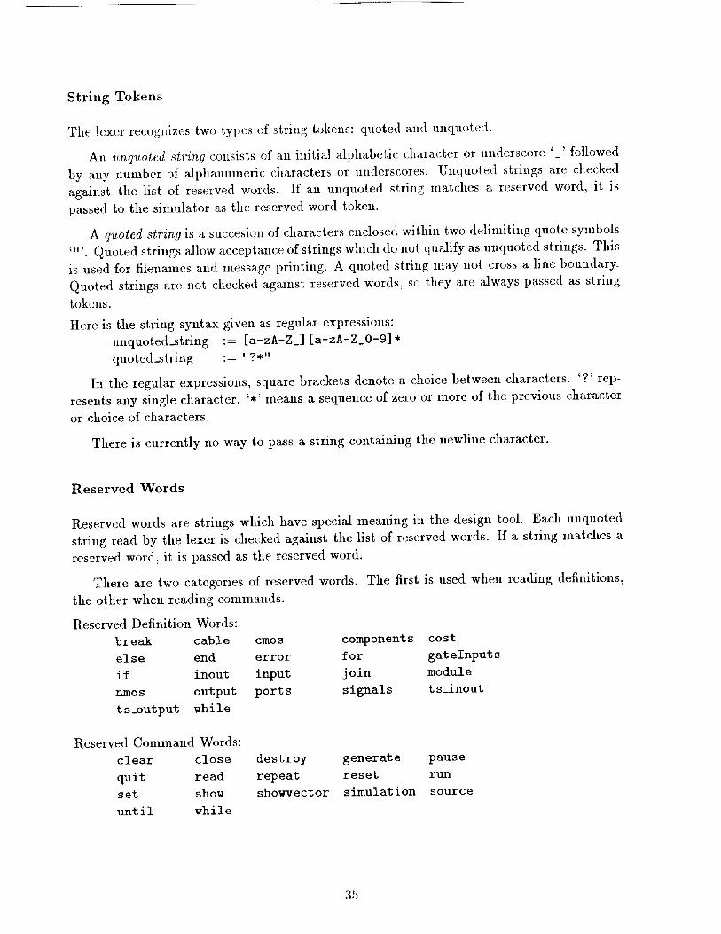
String Tokens

Tile lexer recognizestwo types of string tokens: quoted and unquoted.

An unquoted string consists of an initial alphabetic chara('ter or underscore '_' followed

by any number of alphanunmric characters or underscores. Unquoted strings are checked

against the list of reserved words. If an unquoted string matches a reserved word, it is

passed to the simulator as the reserved word token.

A quoted string is a succesion of characters enclosed within two delinfiting quote symbols

'"'. Quoted strings allow acceptance of strings which do not qualify as unquoted strings. This

is used for filenames and message printing. A quoted stri_g may not cross a line boundary.

Quoted strings are not checked against reserved words, so they are always passed as stringtokens.

Here is the string syntax given as regular expressions:

unquoted_string := [a-zA-Z ] [a-zR-Z 0-9]*

quoted_string := "?*"

In the regular expressions, square brackets denote a choice between characters. '?' rep-

resents any single character. '*' means a sequence of zero or more of the previous characteror choice of characters.

There is currently no way to pass a string containing the newline character.

Reserved Words

Reserved words are strings which have special meaning in the design tool. Each unquoted

string read by the lexer is checked against the list of reserved words. If a string matches a

reserved word, it is passed as the reserved word.

There are two categories of reserved words. The first is used when reading definitions,

the other when reading commands.

Reserved Definition Words:

break cable cmos components cost

else end error for gateInputs

if inout input join module

nmos output ports signals ts_inout

ts_output while

Reserved Command Words:

clear close destroy generate pause

quit read repeat reset run

set show showvector simulation source

until while

35

Numeric Tokens

Four types of numeric tokens are recognized by the lexer: binary, octal, decimal, and hex-

adecimal. These correspond to numbers in base 2, 8, 10, and 16 respectively.

Binary, octal, and hexadecimal numbers have '0' as their initial character. The secoud

character specifies the base of the number.

'b' or 'B' specifies a binary number. This is followed by a sequence of the characters

_0 _ or _1 _,

'o' or '0' specifies an octal number. This is followed by a sequence which may contain

characters corresponding to the numbers 0-8.

'x' or 'X' specifies a hexadecimal number. This is followed by a sequence which may

contain characters corresponding to the numbers 0-9 or alphanumeric characters in the

range a-f (upper or lower case). The characters a-f represent the decimal values 10-15

respectively.

If the second character does not fall into the above categories or if the leading character

is a number which is not '0', the numeric token is a decimal number. A decimal number is

a sequence of characters, each of which corresponds to a number in tim range 0-9.

Each syntax is repeated below as a regular expression.

binaryammber := 0 [bB] [01] *

octalmumber := 0 [oO] [0-8]*

hexadecimM_nnmber := O[xX] [O-9a-fA-F]*

decimalmumber := [0-9] [0-9]*

In the regular expressions, square brackets denote a choice between characters. '*' means

a sequence of zero or more of the previous character or choice of characters.

All types of numeric tokens are interpreted as having the most significant digit on theleft.

36

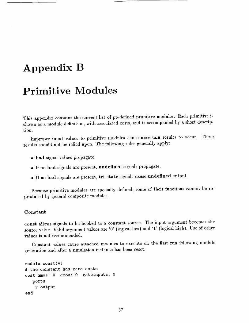
Appendix B

Primitive Modules

This appendix contains tile current list of predefined primitive modules. Each primitive is

shown as a module definition, with associated costs, and is accompanied by a short descrip-

tion.

hnproper input values to primitive modules cause uncertain results to occur. These

results should not be relied upon. Tile following rules generally apply:

* bad signal values propagate.

• If no bad signals are present, undefined signals propagate.

• If no bad signals are present, tri-state signals cause undefined output.

Because primitive modules are specially defined, some of their functious cannot be re-

produced by general composite modules.

Constant

const allows signals to be hooked to a constant source. The input argument becomes the

source value. Valid argument values are '0' (logical low) and '1' (logical high). Use of othervalues is not recommended.

Constant values cause attached modules to execute on the first run following module

generation and after a simulation instance has been reset.

module eonst(v)

# the constant has zero costs

cost nmos: 0 cmos: 0 gateInputs: 0

ports

v output

end

37

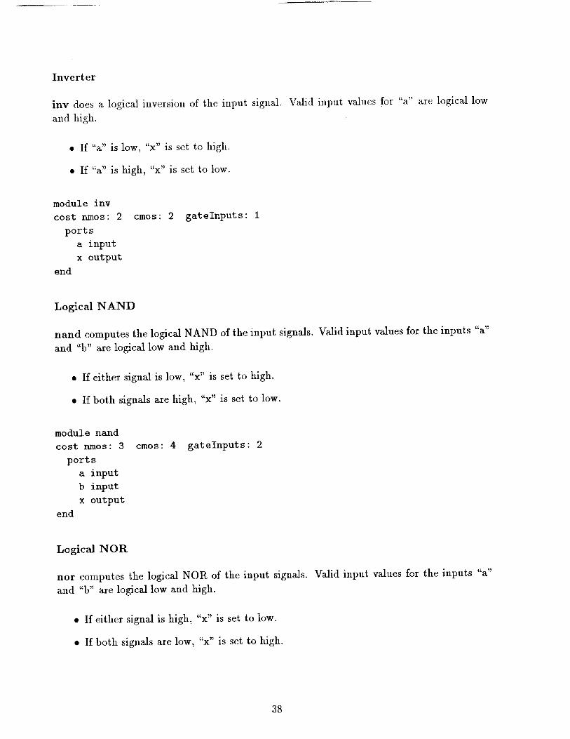
Inverter

inv does a logical inversion of the input signal. Valid input values for "a" are logical low

and high.

• If "a" is low, "x" is set to high.

• If "a" is high, "x" is set to low.

module inv

cost nmos: 2

ports

a input

x output

end

cmos: 2 gateInputs: i

Logical NAND

nand computes the logical NAND of the input signals. Valid input values for the inputs "a"

and "b" are logical low and high.

• If either signal is low, "x" is set to high.

• If both signals are high, "x" is set to low.

module nand

cost nmos: 3

ports

a input

b input

x output

end

cmos: 4 gateInputs: 2

Logical NOR

nor computes the logical NOR of the input signals. Valid input values for the inputs "a"

and "b" are logical low end high.

• If either signal is high, "x" is set to low.

• If both signals are low, "x" is set to high.

38

module nor

cost nmos: 3

port s

a input

b input

x output

end

cmos: 4 gateInputs: 2

Delay

delay simply propagates a signal value with a time delay. The output signal is set to the

input signal, regardless of the value. The input argument is the time to delay the output,

which must be a positive number.

The cost of a delay is represented as a pair of inverters.

module delay(delta)

cost nmos: 4 cmos: 4

ports

d input

q output

end

gatelnputs: i

Transmission Gate

trans_gate sets the output "q" to the value of the input "d" when enabled with the enable

signals "el" and "e2". When not enabled, "q" is set to the tri-state value. The transmission

gate is a dual-rail model_ which means %1 '_ should always be the logical inverse of "eT'.

• When "el" is high ("e2" is low), "q" gets the value of "d".

• When "el" is low ("e2" is high), "q" gets the tri-state value.

"q" must be hooked to a bus signal. This means that all ports which output to the bus

nlust be typed as tri-state. In particular, only trans_gate outputs and SRAM data lines

may output to the sa*lm signal as "q".

module trans_gate

cost nmos: i cmos: 2

ports

d input

el input

e2 input

end

q ts output

gatelnputs: 2

39

Positive Latch

posLatch is a single bit of non-volatile memory. It uses 'T' to control when data is read

into nlemory front "d'. The value in memory is output through "Q".

• When "1" is low, the latch holds state.

• When "1" is high, the memory value (and "Q") is set to the vMue of "d".

module posLatchcost nmos: 8 amos: I0

ports

d input

1 input

O output

end

Negative Latch

negLatch is a single bit of non-volatile memory. It uses "1" to control when data is read

into memory from "d". It is called a negative latch (as opposed to positive latch) because

the sense of the latch signal "1" is reversed. The value in memory is output through "Q".

• When 'T' is low, the memory value (and "Q") is set to the walue of "d".

• When "1" is high, the latch holds state.

module negLatch

cost nmos: 8 amos: I0

ports

d input

Ib input

Q output

end

Static RAM

SRAM is memory for simulation instances. A static RAM module takes two arguments:

the amount of memory and the number of bits in the word. It reads and stores data in

addressable memory based on its control signMs "rw" and "e". "e" enables the RAM for an

operation, and "rw" selects whether the operation reads fronl or writes to memory.

• If "e" is low, the memory does nothing.

4O

• If "e" is high, the melnory doesthe specifiedoperation.

• If "rw" is low, the operation is a write.

• If "rw" is high, tile operation is a r(_ad.

Tile signalsin "D" must behookedto busses.This meansall ports which output to eachbus must be typed as tri-state. In particular, only trans_gate outputs and other SRAMdata lines may output to thosebusses.

There is currently no way to preloaddata into the memory.All data must be written tomemorybeforeit is used.

Data widths larger than 32 bits arenot supported.

module SRAM(amount, width)

port s

rw input

e input

A [i:amount] input

D [I:width] ts_inout

end

Dynamic Memory Test

D_test is used to simulate dynamic RAM in conjunction with the static RAM module

SRAM. It keeps track of the last time data was written to the address, however D_test

does not actually store the data. If data is used too long after it has last been written, an

error message is generated.

The "rw" and "e" lines work as described for the static RAM.

module D_test (amount)

ports

rw input

e input

h [I :amount] input

end

41

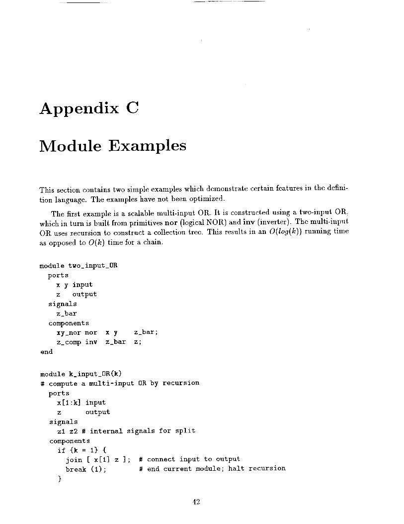
Appendix C

Module Examples

This section contains two simple examples which demonstrate certain features in the defini-

tion language. The examples have not been optimized.

The first example is a scalable multi-input OR. It is constructed using a two-iuput OR,

which in turn is built from primitives nor (logical NOR) and inv (inverter). The multi-input

OR uses recursion to construct a collection tree. This results in an O(log(k)) running time

as opposed to O(k) time for a chain.

module two_input_0R

ports

x y input

z output

signals

z_bar

components

xy_nor nor

z_comp inv

end

x y z_bar;

z_bar z;

module k_input_0R(k)

# compute a multi-input OR by recursion

ports

x[l:k] input

z output

signals

zl z2 # internal signals for split

components

i_ {k : i} {

join [ x[l] z ];

break (i);

}

# connect input to output

# end current module; halt recursion

42

# compute split informationkl <- k/2;k2 <- k - kl;

# split in half and recurse on both parts.zl_comp k_input_OR(kl) x[l:kl] zl;

z2_comp k_input_0R(k2) x[kl+l:k] z2;

# recombine parts

z_comp two_input_0R

end

zl z2 z;

This example uses recursion to split the tree into two subtrees, and a two_input_OR to

recombine the subtrees. Recursion is halted when the subtree has only a single input. This

is done by using break to end the module definition.

The second example is a variable length MIN circuit. It uses a for loop to join a chain

of single-bit MIN modules.

module two_input_AND

ports

x y input

z output

signals

z_bar

components

xy_nand nand

z_comp inv

end

x y z_bar;

z_bar z;

module a_gre_b

# set z to one if a is greater than b ((a = I) & (b = O))

ports

a b input

z output

signals

b_bar

components

b_inv inv

end

b b_bar;

z_comp two_input_AND a b_bar z;

module MIN

43

# compute MIN based on input values and selection inputs

# compute selection outputs for chaining

# (sxi = i) -> choose x as the MIN

# (syi = I) -> choose y as the MIN

# sxi = syi = i is an impossible state

ports

x y input

z output

sxi syi input

sxo syo output

signals

zl z2 z3

sxi_har syi bar

x_gre_y y_gre_x

sxo_e syo_e

components

# compute the min value z

x_sel two_input_AND

y_sel two input_AND

xy_and two_input_AND

z_comp k_input_OR(3)

# select control input

# select control output

# used to find out which data input is greater

# contains new select information

x sxi zl;

y syi z2;

x y z3;

zl z2 z3 z;

sxi_inv inv sxi sxi_bar;

syi_inv inv syi syi_bar;

# check if values are not equal

x_gre_y_comp a_gre_b x y x_gre_y;

y_gre_x_comp a_gre_b y x y_gre_x;

# compute new select information

sxo_e_comp two_input_AND y_gre_x syi_bar sxo_e;

syo_e_comp two_input_AND x_gre_y sxi_bar syo_e;

# compute output selects

sxo_comp two_input_0R

syo_comp two_input_DR

end

sxi sxo_e sxo;

syi syo_e syo;

MIN uses inforinadon from the input select lines or by comparing the two signals x and

y to compute the output z and the output select lines. Note that reversing the order of

signals connected to the ports of the circuit a_gre_b changes its function.

module k_bit_MIN(k)

# compute a variable length MIN circuit by iteration of

44

# a chainable single bit MINports

x[l:k] y[l:k] inputz[l:k] output

signalssx[O:k] sy[O:k] low

components# Turn off initial select signals

low_gen const (0) low;

join [ low sx[O] sy[O] ];

# Chain MIN circuits together

for i = l,k

bit[i] MIN x[i] y[i] z[i]

end

sx[i-1] sy[i-1] sx[i] sy[i];

The chain is initialized by connecting the first set of select inputs to the low signal. The

last set of select outputs is left unconnected.

45

Appendix D

Error Messages

Error messages each have an associated field which describes its type. The error type is used

to identify groups of messages for special consideration. Upon startup, a print mask and

a halt mask are read from the slmre file. The print mask specifies error types which are

printed. The halt mask specifies error types which halt design tool execution. Each message

that halts execution is automatically printed.

Following is a lis_ of error masks and their associated groupings. Each mask is given as

an octal constant.

000001L

000002L

000004L

000010L

O00020L

000040L

000100L

000200L

000400L

001000L

002000L

004000L

010000L

020000L

Race condition during a simulation run

Corrected parsing error

Warning

Redefinition of a cable or module

Reference to undefined cable or module

Conflicting definitions

Uncorrectable parsing error

Module generation halted

Error in primitive moduleBad data found

Error statement executed

Memory allocation error

Error external to program

Inconsistency in program

46

September 91

DESIGN AND ANALYSIS OFEFFICIENT HIERARCHICAL

INTERCONNECTION NETWORKS*

S. Wei and S. Levy

LCSR-TR-167

Laboratory for Computer Science Research

Hill Center for the Mathematical Science

Busch Campus, Rutgers University

New Brunswick, New Jersey 08903

*This work was supported by the Defense Advanced Research Projects Agency

and the National Aeronautics and Space Administration under NASA-Ames

Research Center grant NAG 2-668.

Design and Analysis of Efficient Hierarchical

Interconnection Networks

Sizheng Wei and Saul Levy

Department of Computer Sdence

Rutgers University

New Brunswick, NJ 08903

Footnotes

The authors axewith the Department of ComputerScience,RutgersUniversity,

New Brunswick, NJ 08903.

This work wassupported by the Defense Advanced Research Projects Agency

aad the National Aeronautics and Space Administration under NASA-Ames

Research Center grant NAG 2-668.

Index Terrors -- Hierarchical networks,

Performance analysis, Traffic distributions.

Lntercormection networks,Multic°mputer systems,

Abstract

]5.ierarchical interconnection networks exploit locality in communication to reduce the number

of links in the networks. In this paper, we propose a class of general hierarckical interconnection

networks for message-passing architectures which are designed using a new approach -- choosing the

appropriate number of interface nodes and the appropriate size of dustars based on performance and

cost-effectiveness measures. We show that the approach considerably reduces not only interclnster

traffic density but also intracluster traffic density. It also enhances tke fault tolerance capability of

the networks. We present a performance analysis of the hierarchical networks based on both static

and queueing analyses.

The asymmetric topology of a hierarchical network may degrade performance and reliability

because of some heavy traffic links. The traffic distributions in hierarchical networks are thus

important, but so far there has been very little analysis of the problem. We analyze the traffic

distribution on two-level networks and try to reveal the relationship between traffic density and

other performance and cost-effectiveness measures. In addition, we investigate in detail how to con-

struct a cost-effective hierarchical network by setting appropriate design parameters. An associated

algorithm is developed.

1 Introduction

Multicomputer systems with hundreds or thousands of processors are expected to have the

most potential for the next generation of supercomputers. The intercormection networks in these

multicomputer systems play a very important role in determining system performance. Message-

passing organization is preferable for these systems due to the simplicity of communications among

processors [71 [9] [161 [181.

For a very large system, a critical problem of the interconnection network is that the number of

links needed becomes prohibitively large. To tackle the problem, hierarchical in_erconnec*ion ne_-

works, which exploit locality in communication to reduce the number of Links, have been proposed

in the hteratttre. Some examples are Hierarchical Intereonnection Networks (ttINs) [5], Hypernet

[10], Hierarchical Cubic Network (HEN) [8], a duster structure using shared busses as the basic

interconnection media [20], Hierarchical Memory Structure (HMS) using crossbar switches [14],

and a two-level mesh hierarchy scheme [3]. Also several systems have been made with hierarchical

interconnection networks, such as Cm* [19] and Cedar [t2]. Among these networks, most are based

on some specific topologies such as hypereube, mesh, bus, etc. Few analyses have been made for

general hierarchical networks.

The HINs proposed in [5] are a class of hierarchical networks for message-passing systems. A

HIN is constructed in the following way: All nodes in the system are grouped into dusters and each

cluster of nodes is linked internally by a level 1 network. One node is selected from each cluster to

act as an interface node. These interface nodes may be linked by a level 2 network, or they may

be themselves grouped into clusters, with each cluster linked by a separate level 2 network. In the

latter case, one node from each cluster at level 2 is selected as an interface node to construct the

level 3 network, and so on. A performance analysis was given in [5] for several examples of two-level

HINs. It was shown that a HIN is more cost-effective than its non-hierarchical network counterpart

ff locality in communication exists, i.e., the ItIN gains more performance benefit per unit cost. The

authors also indicated the disadvantages of IlINs_ including high traffic density over intercluster

links and some intrachister links (a potential degradation in performance) and diminished fault

tolerance capability because of the single interface node in each cluster. Replication of intercluster

links and more sophisticated routing algorithms were suggested to alleviate the congestion on these

links.

In this paper, we propose a class of general hierarchical intercormection networks for message-

passing architectures which are designed using a new approach. Unlike the HINs in [5], the proposed

hierarchicalnetworksareallowedto selectanynu2nberof nodesfrom eacl_clusteras interface

nodes. The optimal numberof interfacenodesand the optimal sizeof clustersaredeternfinedbasedonperformanceandcost-effectivenessmeasures.Wewill showthat increasingthentm_berof

interfacenodesin eachdusterusingthe samenumberof lhtksnot only reducesthe sameamomltof interclustertrafficdensityasreplicationof linksdoes,but alsoreducesa considerableamountof

intraclustertrafficdensity,sothat the intraclustertraffic canbebalanced.In addition,it enhances

the fault tolerancecapabilityof thenetworks.

A major problemwith a hierarchicalnetworkis that the networkis usuallyasymmetriceven

if eachduster is symmetric, which results in some heavy traffic links that may become potential

communication bottlenecks. Where would congestion take place and how can it be alleviated? What

is the relationship between traffic density and other performance and cost-effectiveness measures?

To answer these questions one must analyze traffic distributions in hierarchical networks which is

difficult. Therefore, one of the objectives of this work is to analyze the traffic distributions so that

we can gain a better insight into hierarchical networks.

We evaluate the performance of the proposed networks in terms of diameter, average internode

distance, traffic density over links, and queueing delay with contention. We also analyze in detail

how to design a cost-effective hierarchical network by choosing appropriate design parameters. An

associated algorithm is developed.

This paper is organized as follows: Section 2 outlines the construction of the proposed hier-

archical networks. In Section 3, performance and cost-effectiveness measures for the hierarchical

networks are studied. Some examples of the hierarchical networks are analyzed and compared in

Section 4. Section 5 analyzes how to determine the design parameters to construct a cost-effective

network. Finally, the concluding remarks appear in Section 6.

2 Construction of hierarchical networks

The construction of the proposed hierarchical networks can be described as follows. Let N be

the total number of nodes in a hierarchical network. The N nodes are divided into KI clusters

of N/K1 nodes each. Each cluster of N/K1 nodes is connected to form a level 1 network. For

convenience of analysis, we assume that Ki evenly divides Ki-1 at level i, with initially K0 = N,

and every cluster at the same level is of the same size. The nodes in every cluster are ordered in

the same way, i.e., the corresponding nodes in different clusters have the same internal address.

Then, /1 nodes, t <_ I1 < N/K1, from each cluster are selected to act as the interface nodes. To

be symmetric, the same I1 interface nodes from each cluster are selected, t:or example, if the fL_

and jth nodes in cluster 1 are selected, the i eh axed j e;`nodes in all other clusters are also interface

nodes. There axe total of Ix x K1 interface nodes at level 1.

To construct level 2 networks, these interface nodes are first divided into Ii groups. Each group

consists of Kt nodes which are from K1 different dusters, i.e., one from each cluster with the same

internal address. Note that all groups are independent, i.e., there is no connection between any

pair of nodes which belong to different groups. Then, the K1 nodes of each group are again divided

into K2 dusters of K1/K_ nodes each. Each duster is connected to form a level 2 network, and I2

nodes, 1 < I_ <_ K1/Ks, axe selected as the interface nodes to construct level 3 networks, and so

Oil..

The interconnection networks used to construct clusters at different levels may have the same or

different topologies. Here it is assumed that all clusters at the same level are of the same topology.

There are K1 clusters at level 1, 11K_ dusters at level 2, hhKs clusters at level 3, and so on. Some

examples of proposed networks are shown in Fig. 1. Fig. 1 (a) is a two-level network with N = I6,

/(1 = 4,/1 = 2, and/(2 = 1, and each cluster at level 1 is a completely connected network (CC)

and that at level 2 is a binary hypercnbe network (BH). In Fig. 1 (b), both levels are constructed

using BH with N = 32,/(1 = 4,/1 = 2, and Ks --- 1.

The HINs described in [5] are special eases of the networks described here, i.e., all Ii axe equal

to 1. In addition, some one-level networks can be constructed hieraxchically. For example, an

ordinary binary hypercube network of size N is a two-level network with I1 -= N/K1 and Ks = 1,

where hypercnbe connection is used at both levels.

In the following analysis, all hierarchical networks are restricted to two levels. This is because

the analysis for the two-level networks is relatively simple and the results can be extended to the

networks with more levels. Also it is pointed out in [5] [6] that two is a pragmatic choice for the

number of levels in the hierarchy. For a two-level network, we assume that Ks is always 1, i.e., only

one cluster for each group of interface nodes.

3 Performance and cost-effectiveness measures

We now analyze the performance and cost-effectiveness of the hierarchical networks. We first

give some definitions and make some assumptions. Let

N -- the total munber of nodes in a hierarchical network;

L (i) -- the total ntunher of links at level i;

L! i) -- the number of hnks in a cluster at level i;

L -- the total number of links in a hierarchical network;

K1 -- the number of dusters at level I;

I1 -- the number of interface nodes selected from each duster at level 1;

Din(i) -- the diameter of a duster at level i;

Dm -- the diameter of a hierarchical network;

AD(i) -- the average internode distance of a duster at level i;

AD -- the average internode distance of a hierarchical network;

TD(/_ ) , -- the highest traffic density over links in a duster at level i;

TD_ -- the highest traffic density over links in a hierarchical network;

A -- the message generation rate at each node;

j_(i} -- the message arrival rate at the level i links which cause the longest delay at thisllruk,maz

level;

/_(i) __ the message processing rate of each link at level i;

W(,_ -- the longest average delay at level i links;

Wmax -- the longest average delay at links in a hierarchical network;

p -- the probability that the source and destination nodes of a message are in the same level

1 duster. (For comparison, we adopt a similar message distribution model used in [5].) Thus,

(1 - p) is the probability that the source and destination are in different clusters. The larger the

value of p for a given duster size, the stronger the locality of communication. It is assumed that

both intracluster and intercluster communications are uniformly random, i.e., a source node sends

an intracluster message to each other node in its cluster with equal probability and a source node

sends an interduster message to each node in other cluster with equal probability. Note that the

case of a node sending messages to itself is excluded.

The four important performance measures -- diasneter, average hlternode distance, traffic

density over finks, and queaeing delay with contention are derived below. We also give the cost-

effectiveness measures and briefly show the fault tolerance capability of the hierarchical networks.

3.1 Diameter

The diameter of a network is the maximum internode distance between any two nodes. For a

two-level hierarchical network, the diameter is

Dm<2Dm (1}+Din(2); ifl </1 <N/Kz

Dm= Din(1) + Din(2); if h = N/K,

(1)

The formula above is derived based on the following facts:

i) /1 = 1: If a duster at hvd 1 is constructed by a symmetric network (the network looks

identical when viewed from any of its vertices) such as hypercube and ring, the Din0) is the

distance between the interface node and the node farthest away from it. Considering the two

clusters for which their interface nodes at level 2 axe farthest away from each other, we can easily

find that 2DmO) + Din(2) is the diameter of the hierarchical network. For an asymmetric network

at level I such as a binary tree, the Din(1) may be greater than the distance from the interface

node to any other node in the duster. In this ease, Dm< 2Drn(1) + Din(2).

ii) 2 < I1 < N/K1: Usually Dm< 2Din(l) + Din( 2} because more interface nodes give more

alternative paths between any two nodes. However, for some type of networks such as completely

connected network used at level 1, the distance between two non-interface nodes in the two dusters

which axe farthest away from each other is always 2Din(1) + Din{2). From i) and ii), we have the

inequality above.

ifi) I1 = N[KI: In this case, every node is an interface node. A message from a source node in

duster i to its destination node in duster j, i _ j, can go through a path which does not include

any link in duster i. Thus_ the diameter is at most Din(1) + Din(2). On the other hand, if cluster

i is farthest away from cluster 3" and the position of the destination node in cluster j corresponds

to that of the node in cluster i which is farthest away from the source node, the distance between

the source and destination is at least Din(1) + Dm(_). The equation above is thus proved.

3.2 Average internode distance

Like diameter, average interr_ode distance is a fvJldamental prol)erty of a topology. Average

internode distance is the expected number of Iink traversals a "typical" message needs to reach its

destination. It is a better indicator of message delay than the diameter [17]. Average internode

distance depends on the message distribution which describes the probability of message exchanges

among different nodes.

A hierarchical network is usually not symmetric even if the networks used to construct clusters

at each level are symmetric. As a result, the average internode distance from different source nodes

to all other nodes can be different. For example, the average internode distance from an interface

node to MI other nodes will be shorter than that fzom a non-interface node. However, if we take

the average of the average internode distances over all nodes, the average internode distance of a

two-level hierarchical network can be computed as follows:

AD__p. AD (1)+(1-p)(2AD (1}+AD(2}); ifl</1 <N[K1 (2)AD = P" AD(') + (1 - p)(ADO) + AD(2)); if I, =/_/K 1

The derivation of the formula is similar to that of the diameter.

3.3 Traft]c density

Tra]_ density over links is another important performance measure which reflects link utiliza-

tion. The analysis of traffic density is important, especially for asymmetric networks, because this

measure can indicate potential communication bottlenecks. So, it may be a better performance

measure than diameter or average internode distance for asymmetric networks. Low traffic density

is preferable. Traffic density is measured in terms of the average number of messages per link per

unit time, given that each node issues one random message per unit time (Here _random" means

that the destination distribution of the messages is uniform).

Since a hierarchical network may be asymmetric, the traffic density over each link in a cluster

can vary. Also the traffic density over a link at level 1 may be different from that over a link at

level 2. Here the analysis is concentrated on the Winks with the highest traffic density, because they

are potentially the bottlenecks and they determine the worst case in communication delay. For

simplicity, it is assumed that the networks used to construct clusters at each level are symmetric.

Note that traffic density is related to the traffic distribution pattern and the routing algoritttm

employed for the network,

The highest trai_c density over tile lil_ks at level 1: It is easy to see that the links directly

connecting interface nodes would be the links with the tfighest traffic density (Prom now on, we

only consider the traffic density over these links). The traffic density, TD_)_:, over these links

consists of three parts:

TD (1) -- Traffic density generated by intraduster communications;local

TD_ -- Traffic density generated by outgoing messages to other clusters;

TD!_ ) -- Traffic density generated by incoming messages from other clusters.

When the message distribution within a duster is uniform, i.e. 1 when every node in the cluster

generates a random message per unit time and every message behaves statistically identically,

Tn(1)_t_o_ can be computed using ADO):

TDO) pN ADO)

lo¢_z- K1 × L! 1)(3)

which means that the total number of traversals made by all the pN/K1 messages are shared equally

by L! l) links in the cluster. Thus, TD[I)o_ over every link in the duster is the same.

To calculate the traffic density generated by intercluster messages, it is necessary to specify a

routing strategy first. A natural and simple routing strategy is to divide a cluster into I1 disjoint

subclusters of equal size (e.g, divide a cube into subcubes), each containing an interface node.

When a node wants to send a message to another cluster, it first sends the message to the interface

node in its subcluster. In this way, the interface node in a subduster is responsible for sending out

the messages generated by all the nodes in the subeluster. For the incoming messages from other

dusters, however, the interface node has to forward them to all the nodes in the whole cluster.

Since each cluster is symmetric, the amount of traffic through each interface node is the same.

Based on this routing strategy, the TDOo_ ) over a link connecting an interface node is

N 1)ql, 1<I1<_ _ N<') = (1 - P)()clrl (4)

where I represents the I t_ link connecting the interface node and qi is a fraction that gives the

percentage of outgoing messages through the I th link over all the outgoing messages generated by

the subclnster (except the interface node). The range of the values of l depends on the network

topology, but it is at least 1. The value of ql depends on both network topology and routing

algorithm. If the 1 links equally share the outgoing traffic, all values of ql are identical. Note that

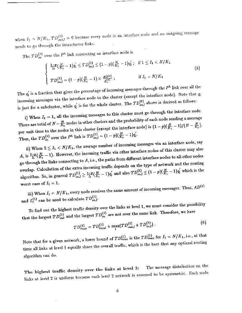
when I1 = N/K1 TD (1) = 0 because every node is an interface node and no outgoing message, out,/

needs to go through the intracluster links.

The TD_ ) over the l th link connecting an interface node is

t

k=arN '_TD O) <(l_p)(_i__l)ql.z, t_-i(- 1)ql < i,,,t -

(5)ADO)

= (1 - l) × ;

The ql is a fraction that gives the percentage of incoming messages through the lth link over all the

incoming messages via the interface node to the duster (except the interface node). Note that q1

is just for a subduster, while qL is for the whole duster. The TD t above is derived as follows:

i) When/1 = 1) all the incoming messages to this cluster must go through the interface node.

There are total of N- _ nodes in other clusters and the probability of each node sending a message

per unittime to the nodes in thisduster(exceptthe interfacenode) is(1- p)(_ - 1)/(N - N_)-

Thus,theTD 2 ova the l" isTD(1),.,-- (1- - 1)ql

ii) When 2 _ It < N/Kt, the average number of incoming messages via an interface node, say

1-_[/v _ 1). However, the incoming traffic via other interface nodes of this cluster may alsoA, is h _R7

go through the links connecting to A, i.e., the paths from different interface nodes to all other nodes

overlap. Calculation of the extra incoming traffic depends on the type of network and the routing

__=e_N 1)q i and also TD_!I < (1 - p)(_ - 1)q_ which is thealgorithm. So, in general TD}_!, > I, tR7 -

worst case of Ii = 1.

iii) When/1 = N[K1, every node receives the same amount of incoming messages. Thus, ADO)

and L! 1) can be used to calculate TD O)in,l"

To find out the highest traffic density over the links at level 1, we must consider the possibility

'Pr)(l) TD_ ) are the link. Therefore, we havethat the largest _.--out and the largest not over same

TD (t) = TD}2,. + max(TD_{_ +'_n(z) Xl

Note that for a given network, a lower bound of TD(ml):: is the TD(ml):: for/1 = N/Kt, i.e., at that

time all links at level 1 equally share the overall traffic, which is the best that any optimal routing

algorithm can do.

The highest traffic density over the links at level 2: The message distribution on the

links at level 2 is uniform because each level 2 network is assumed to be symmetric. Each node

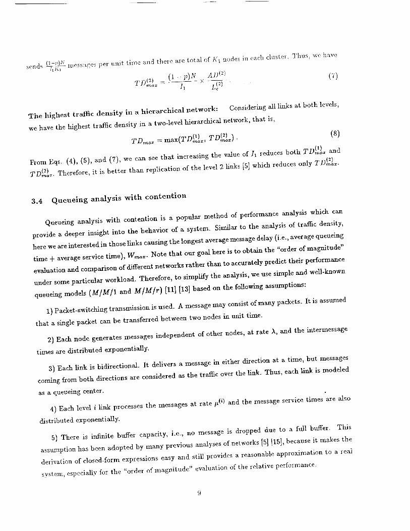
I 1-p)/_Tsends _ messages per unit time and there are total of K1 nodes in each cluster. Thus, we have

- × -- (r)

The highest traffic density in a hierarchical network: Considering all links at both levels,

we have the highest traffic density in a two-level hierarchical network, that is,

From Eqs. (4), (5), and (7), we can see that increasing the value of I, reduces both TD!2)_, and

TD(2,_)=. Therefore, it is better than replication of the level 2 links [5] which reduces only TD#}_=.

3.4 Queueing analysis with contention

Queueing analysis with contention is a popular method of performance analysis which can

provide a deeper insight into the behavior of a system. Similar to the analysis of traffic density,

here we are interested in those links causing the longest average message delay (i.e., average queueing

time + average service time), W,_x. Note that our goal here is to obtain the "order of magnitude"

evaluation and comparison of different networks rather than to accurately predict their performance

under some particular workload. Therefore, to simplify the analysis, we use simple and well-known

queueing models (M/M/1 and M/M/r) [1I] [la] based on the following assumptions:

1) Packet-switching transmission is used. A message may consist of many packets. It is assumed

that a single packet can be transferred between two nodes in unit time.

2) Each node generates messages indepeitdent of other nodes, at rate )_, a_d the intermessage

times are distributed exponentially.

3) Each link is bidirectional. It delivers a message in either direction at a time, but messages

coming from both directions are considered as the traffic over the link. Thus, each link is modeled

as a qneueing center.

r

4) Each level i link processes the messages at rate #(i) and the message service times are also

distributed exponentially.

5) There is infinite buffer capacity, i.e., no message is dropped due to a full buffer. Tiffs

assumption has been adopted by many previous analyses of networks [5] [15], because it makes the

derivation of closed-form expressions easy and still provides a reasonable approximation to a real

system, especially for the "order of magnitude" evaluation of the relative performance.

6) The routing strategy is the sai!ie as we used for tlle analysis of traffic det_sity, i.e., wimn a

node needs to send a message to another cluster, it first sends the message to the interface node in

its subcluster.

The longest delay at level 1: Each level 1 link is modeled as an M/M/1 queueing center.

It is easy to see that the TD_)_ derived before can be directly used to derive the message arrival

rate at the links which cause the longest delay at level 1 (The difference is that for traffic density

we assume that on the average each node issues one message per unit time, while now we assume

that each node issues )_ messages per unit time). Thus, we have

llnk,rnax

The longest delay at level 1 links is

ix(i) A(i)-- link,*na_

#(_) _ ),. T D(J_)_ "(9)

The longest delay at level 2: Each level 2 link is also modeled as an M/M[1 queneing center.

Using TD(2_)_ to compute the message arrival rate at level 2 links, we have the following result:

W(22:_,,_uI _ 1 1#(2) _(2) #(2) X.TD_) ' (I01

-- "'link,ma_

where the subscript "mul" is for the approach of choosing multiple interface nodes (we will use

"rep" for replicating level 2 links).

For comparison, we also consider the delay for the approach of replicating level 2 Bilks in [5].

Each group of r-replicated links can be modeled as an M/M/r queueing center. TD_}a: can still

be used to compute ._}_/¢,,_., but we should always let I, = 1 when we compute TD(2._)_ (It is also

the same for computing TD_ ), and W2)z). Using the formulas for M/Mfr model [21, we have

link,maz

.X(_) T D(_) .X(2)link,max _ " llnk,rr_az t£

#(2) tz(2) ' P - t2(2) - r r '

r!

_: + (1 , _-_-i ,,- ,-- - P) 2_,,_=o -W-

10

[ ]

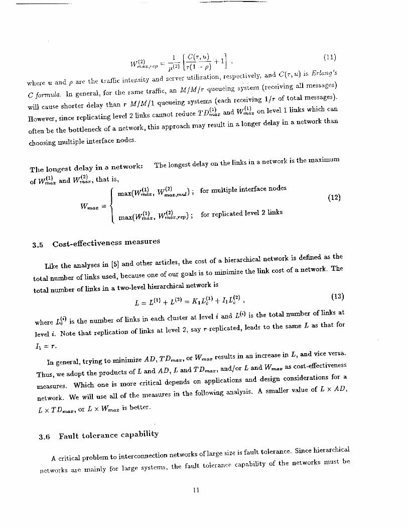
where u and p are the traffic intensity and server utifization, respectively, and C(r, u) is Erlang'.s

C formula. In general, for the same traffic, an M/M/r queueLag system (receiving all messages)

will cause shorter delay than r M[M/1 queueing systems (each receiving 1/r of total messages).

However, since replicating level 2 links cannot reduce TD(1,_):_ and W,(1),_ on level 1 links which can

often be the bottleneck of a network, this approach may result in a longer delay in a network than

choosing multiple interface nodes.

The longest delay in a network:

of W(m21)_ and W(m2_)_, that is,

max(W , ,r max,rau/J

Wmax-_

max(W(lr_}_, Wg)=,,_) ;

The longest delay on the links in a network is the maximum

for multiple interface nodes

for replicated level 2 links

(t2)

3.5 Cost-effectiveness measures

Like the analyses in [5] and other articles, the cost of a hierarchical network is defined as the

total number of links used, because one of our goals is to minimize the link cost of a network. The

total number of links in a two-level hierarchical network is

L = L O) + L (2) = K1L! 1) + IlL! 2) , (13)

where L! i) is the number of links in each cluster at level i and L (1) is the total number of links at

level i. Note that replication of links at level 2, say r-replicated, leads to the same L as that for

AT1 .___ 7""

In general, trying to minimize AD, TD,_,,_:, or W,_ results in an increase in L, and vice versa.

Thus, we adopt the products of L and AD, L and TD,.,_:, and/or L and W,_= as cost-effectiveness

measures. Which one is more critical depends on applications and design considerations for a

network. We will use all of the measures in the following analysis. A smaller value of L x AD,

L x TD,_,::, or L x W,_ is better.

3.6 Fault tolerance capability

A critical problem to intercomneetion networks of large size is fault tolerance. Since hierarchical

networks are mainly for large systems, the fault tolerance capability of the networks must be

11

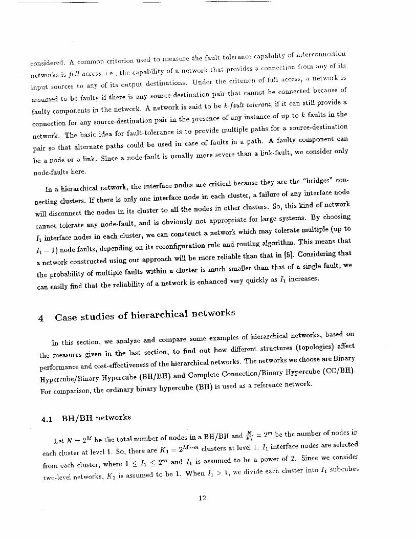
considered. A comallon criterion used to measure the fault tolerance capability of intercomlection

networks is Juli acces.s, i.e., the capability of a network that provides a eomlection from any of its

input sources to any of its output destinations. Under the criterion of full access, a network is

assumed to be faulty if there is any source-destination pair that camlot be connected Because of

faulty components in the network. A network is said to be k-fault tolerant, if it can still provide a

connection for any source-destination pair in the presence of any instance of up to h faults in the

network. The basic idea for fault-tolerance is to provide multiple paths for a source-destination

pair so that alternate paths could be used in case of faults in a path. A faulty component can

be a node or a link. Since a node-fault is usually more severe than a link-fault, we consider only

node-faults here.

In a hierarchical network, the interface nodes are critical because they are the "bridges" con-

necting dusters. If there is only one interface node in each cluster, a failure of any interface node

will disconnect the nodes in its duster to all the nodes in other clusters. So, this kind of network

cannot tolerate any node-fault, and is obviously not appropriate for large systems. By choosing

I1 interface nodes in each duster, we can construct a network which may tolerate multiple (up to

/1 - 1) node faults, depending on its reconftguration rule and routing algorithm. This means that

a network constructed using our approach will be more reliable than that in [5]. Considering that

the probability of multiple faults within a cluster is much smaller them that of a single fault, we

can easily find that the reliability of a network is enhanced very quickly as/1 increases.

4 Case studies of hierarchical networks

In this section, we analyze and compare some examples of hierarchical networks, based on

the measures given in the last section, to find out how different structures (topologies) affect

performance and cost-effectiveness of the hierarchical networks. The networks we choose are Binary

tfypercube/Binary Hypercube (BH/BIt) and Complete Connection/Binary tIypercube (CC/BH).

For comparison, the ordinary binary hypercube (BH) is used as a reference network.

4.1 BH/BH networks

Let N = 2 M be the total number of nodes in a BH/BIt and _ = 2m be the number of nodes in

each cluster at level 1. So, there are K_ = 2 M-m clusters at level 1. /1 interface nodes are selected

from each cluster, where 1 _< /1 <_ 2" and /1 is assumed to be a power of 2. Since we consider

two-level networks, K2 is assumed to be 1. When/1 > I, we divide each cluster into I1 subeubes

12

and each subcube contains an interface node. Based on these assumptions, we have the following

results:

1. The number of links:

L O) = K1L_ 1) = m2 M-1 ,

L (2) = QL (2) = II(M - m)2 M-m-1 ,

LBH/B_ = I,(*) + L (2) = 2M-I(II(Mjm)

F m).

2. Diameter:

DmB_/B.H = (m -- logh) + (M - m) + m = M + m - log/1.

There are two special eases:

i) If 11 = 1, DmBZC/BZ¢ = M + m which is the diameter of the BH/BH networks given in [5].

fl) If I 1 = 2 m, DmBII/BI I = M which is the diameter of the ordinary binary hypercuhe (BH)

networks.

3. Average internode distance:

pr,+(t_p)(m-iog h + M-m 2)ADBHIBH _ _ 2 2 -F

0- p)(M-logh)- +

2 2

4. Trafllc density: We first consider the highest traffic density over the links at level 1, that

is,

TD(1) = 'rD(1} ax (z) + TD_]t )_.= -- to_t + n_ (TDo_t, _

Since each cluster is symmetric, we have

TDO) _ AD(1) - P2 m m2 ,_-1= x m-T _1 x p1 e

To compute TD (1) and TD g)o,,t,t i,_J, we need to specify routing algorithms. Here we consider two

different routing algorithms for comparison:

13

1) The routing algoritlun which evenly distributes the incoming (outgoing) messages over all

links connecting to the interface node in the cluster (sub cluster): There are _z- log I1 links involved

in sharing the outgoing traffic and rn links involved in sharing the h!coming traffic, respectively.r

The, qz = 1/(.. - log11) _d q_= Urn, =d

{ 1 2m

- 1)_v__o_i' , 1 < I_ <

TD(lo_) _ =

0; /I =2 "_

max(l - p, (1-P)(2m-l)_< TD! I) < 0-P)(2_-I)' 1 < 11 < 2"

(1) 2"TD_.,_ = 1 - p ; I, =

Note that TD}I!¢_ cannot be less than 1 - p because now ----,,._eaTD('I}= m ax(TD}l!t) and it should

not he less than that for I1 = 2". Then, for the routing algorithm, we have

J- -a--'locX:l_ T -t Ju'_,c_,en

Two special casesare

i) TDO_)x,_,,_ = p+ :O-p)(='-_) if/1 = I, and

ii) TDP,_)x,e,,e, = 1 ffI1 = 2", which is equal to that for BH.

2) A fixed routing algorithm which is the simplest and most common routing algorithm used

for hypercube systems: The routing code is computed as the bitwise Exclusive-0K of the sot_rce

and destination addresses. The routing code is scanned from the most sihndficant bit to the least

significant bit. By tracing the routing algorithm, we can fred that when 1 </1 < 2'_, more than

_'-* 2" _ 1) go through the linkhalf of the total outgoing messages from a subclustex (--_-- out of T

connecting the interface node and the node whose address differs only in the least significant bit

(e.g., the link between nodes 0000 and 0001 in Fig. 2 (a)). The next link (0000 -- 0010) shares

2"-' 2- _ 1), and so on. Thus, ff we definealmost a quarter of the total outgoing traffic (--9_, out of 7_,

the F h link as the ]ink that comaects two nodes whose addresses differ only in the I th bit position

(starting with the least significant bit as bit 0), we have

_m--l--I

(1 - P)- T_ ; 1<1_<2'_,0<1<m-1

TD O}out,l

0 ; I1 = 2TM

14

Moreover, we also find a similar situatiou for the incoming messages on these links but in reverse

.... of_"-1)goorder. More than a half of total incoming messages to a cluster (=77-_ out through the

link cormecting the interface node and the node whose address differs o_dy in the most sigaificant

bit (e.g., the link between nodes 0000 and 1000 in Fig. 2 (b)). The next link shares almost a

quarter, and so on. ff I1 interface nodes are selected appropriately (e.g., for 2 TM = 16, we select

0000 and 1111 if/1 = 2 (see Fig. 2 (b) and (c)) or 0000, 0101, 1010, and Ili1 if/1 = 4), we can

also have

{ _--(L:E_<TD (D <(l-p)2 _- l<Ia<2",O<l<m-1

I 1 -- in,l -- ) --

TD O) = 1 -p I1 = 2"in,l

It is obvious that TD_,_,_:_ and TD! 11 are not on the same link. By combining TD (l) and_,rn,o,a: o,utj

TD_}_, we can find that

+(l-p)<m(_1)_ +T n<') l<(1-p)(2 "-I+1); 1<I1 <2"I, - tax( T V,,_,t _"i,,,t , - -

q, n0) _ 1 - p; I1 = 2 TMmax(TD_{, + .. _.,,,,,, =l

,VD(Dwhich shows that max(TDO{t +., in,n occurs on link O. Here we have already included theg

incoming traffic via other interface nodes and through link O, which is approximatelyII

Thus, the highest traffic density over the links at level 1 for fixed routing algorithm is

Tn(_) .Tom + m._(TD_{, + rO}_!,)_ rrtaz,]i_ : " to._l t " ' "

Two special cases are

i) _'rD0),_=,a,i= = P + (1 - p)(2 '_-* + 1) ff h = 1, and

ii) TD 0) = 1 if/1 = 2 TM. Note that TDO,_)_: is always 1 (the lower bound) when/1 = 2 TM'-- rnaz,,(iz

no matter what routing algorithm is used. This is true because at that time, the BH/BH is

a BH and overall traffic within a cluster is perfectly balanced.

The traffic density over the links at level 2 can be derived as follows:

AD(2) 1 - p 2MTD(_] _ (1 - p)N x - x

ma=,BHIBH I1 /.,!2) I 1 2M-m -- 1 "

: aodI, : To(:L,../.. - p)2 andr'(gL,..i.. 1- v, r spectively.V_leu II

Finally, we have

.......>,/.. :

15

where TDI_)BH/Btz can be either TD(_)_,e .... or TD!_:,I;_: , depending on wtfich routh_g Mgorithm

is used.

Fig. 5 shows TDm_,BH/Sh" for the two routing algorittuns. We can see that tile two algorit]uns

yield comparable results, i.e., the fixed routing algorithm does not result in a significantly higher

TDnu_:,BH[BH. This is because both algorithms can balance the intercluster traffic on the related

links. To balance the overall traffic (i.e., both interduster and intradnster traffic), we need to

consider some other routing algorithms which can balance the link utilization within clusters, as

described in [4]• However, these algorithms incur more overhead and make control complicated.

5. The longest average delay: The longest average delay in a BH/Btt can be easily computed

using TD,._,BH/BH and the formulas derived in the last section. Since the two routing algorithms

lead to comparable TD,_=, we use TD(12=,BH/BH = --_.,_.=,_q'n(1) to compute W (1)v,u_z,BH/BH.For

W(22=,BIUBtt,__ we consider two cases based on two different approaches for comparison: one choosesw-( _)

multiple interface nodes (denoted as ,, BHfBH,,_lJ and the other replicates level 2 links (denoted

W (_)as BH/BH,repJ"

1) The longest delay at level 1: Each link is modeled as an M/M�1 queueing center.

A0) - A- TD (1}l{nk,,naz -- ra_z,BH/BH I

W(1) = 1

/z(i) -- )_. TD(Az,BH/BH

2) The longest delay at level 2:

i) Multiple interface nodes: Each link is modeled as an M/M/1 queueing center.

A(=)u_,._ = A. TD _,BH/B_ ,

1

W;)HIBH'rnu1 = _(2) _ A" TD(2z,BH/BH "

ii) Replicated links (I_ = 1): Each group of r-replicated links is modeled as an M/M/r

queneing center.

A-TD(_I=,BHIBH u

u = u(2) ' P = 7 '

r!

= + (' ,• - p)2.=o

o

3) The longest delay in a network:

max(W(I_)z,BH/BH, U:(2) ;.• " BH/BH,rnuI) '

Wrnax,BH/BH =

if choosing multiple interface nodes

maX(W =,B :/B W (2)BHIBH,,-cpl " if replicating level 2 links

Note that when replicating level 2 links, the values of TD(1,_}_ and w(D should be computed'' rnaz,BHIBH

with/i = 1. Fig. 6 shows Wr,_,,=,BH/BH for the two different approaches (for replicating level 2

links,/1 means the number of replication) under p = 0.5 and p = 0.8, respectively. Since for given

sizes and workload, the level 1 links of the BH/BH networks with replicated level 2 links saturate

when p < 0.7, Fig. 6 (a) includes the results only for the BH/BH networks which are allowed to

have multiple interface nodes. Also when/1 < 2 (with p -- 0.5) and II = 1 (with p -- 0.8), all of

these networks saturate under the given workload. Therefore, Fig. 6 does not show the results for

these cases.

4.2 CC/BH networks

Similar to BH/BH networks, let N = 2 M be the total number of nodes in a CC/BH and

]_, = 2'* be the mtmber of nodes in each duster at level 1. There are K1 = 2 M-'_ dusters at level

1. /1 interface nodes are selected from each duster, where 1 _< 11 _< 2m. When/1 > 1, any/1 nodes

can be selected as interface nodes because each elustex is a clique. Based on these assumptions, we

have the following restdts:

I. The number of links:

L O) --- K,L (1) -- 2M-1(2 TM - 1),

L (2) = hL (2) = II(M - m)2 M-'_-I ,

= + :) = m)+2" - O.

2. Diameter:

Drncc/B H =

M-m+2; 1<_/-1<2 "_

M-re+l; /-1=2 '_

I7

3. Average internode distance"

/ v + (1 - + 2) ;ADcc/BI: _

v + (1 + 1);

1_<I1 <2 '_'

/1=2 TM

4. Traffic density: The highest traffic density over the links at levd 1 is:

TDO._)=- ,rnO) ± O) '_D(I)- _o_ _ m_ax(TDo-_J + *_i.J' '

where

TriO) - pN ADO) p2 m_lo_- KIL!, ) X - 2'_-a(2'_- i)

,,._,(i}_ TD(1)The m axbt_t,t _ i,,lJ can be computed as follows:

2p×1= .--

2 0_- 1

1) mnO) • Since each duster is a c/ique, a link connecting an interface node shares either-L *J_t,l-

1/('_ - 1) of total outgoing traffic (i.e., the traffic generated by a node in the same subduster) or

nothing (i.e., the traffic generated by a node not in the subcluster). Thus,

1 -p;

Tn0) = 0"

0;

1 _<!i < 2"_and linklconnectingtwo nodes both in the subduster

1 </i < 2'_and linkIconnectingany node not in the subduster

11 =2 "_

2) a, nO). A link connecting an interface node shares 1/(2 '_ - 1) of totM incoming traffic via.'. ,v ln,l.

the interface node. This makes the amount of incoming traffic double on a link connecting two

interface nodes. So, we have

l-p; /_=1

TD_!t = _i1 ' 2 _<Ia <_ 2 _ and link l connecting two interface nodes

_, 2 </1 < 2_ and link I connecting any non-interface node

3) Since TD_{ over the link connecting two interface nodes is 0, we can see that max(TD_{ l +1

18

TriO) "_is not on this kind of li_ks unless Ii = 2_- As a result, we have*"in,l I

+ TDI,_ 3) =

" I1 = 2"n2m--t I

From the derivation above, we have

TD O)maz,CC/BH =

=._ +(1- v)0 + ¼);

=_!a__ JL:e.."_- 2m_ 12m_l

1</i<2 TM

I 1 _-_ 2 TM

The traffic density over the links at level 2 is the same as that of BH/BH networks, that is,

_ 2 _f(1 )N AD (2) 1 - p x

TD(=2.,CClBH - X _ I1 2M-'_ - 1

Finally, we have

TDmax,co/B H = max(TD(l_ } ....... 'r'D(:0x,,.,,.,l_ra _ ._a.=,GClBttJ •

5. The longest average delay: The longest average delay in a CC/BH can be computed as

follows:

1) The longest dday at level I: Each link is modeled as an M/Mil queueing center.

A(x) - A .TD (x)ll.k,ma_ -- m_z,CC/BH '

1

w(22..c I .= ,,(,,_ "

2) The longest delay at level 2: For W(22,,CClBn, we also consider two different cases, i.e.,

amd TAT(=)w(ffc)l_H,,,,,a ""ccmH,,_"

i) Multiple interface nodes: Each link is modeled as an M/M/1 queueing center.

1

W(2}OIBH"_'I = #(2) _ A. TD(2_),cc/BH "

19

ii) Replicatedlinks (Iz = 1): Foachgroupof r-replicatedlinks is modeledas an k_/M/rqueueingcenter.

•TD(2,_,cc/B_r-- UA

= = t_(2) ; _ = 7:

r!_7(r, **) = _,

,'-r.+ (1 - e)

w - ! [ 1]

3) The longest delay in a network:

max(W(i}ni}mz,CC/BH, W(=)'"CG/BH,rauI!_ ," if choosing multiple interface nodes

Wr._z,CC/BH =

ra (W! ),cO/BH ' CC/BH,_J, if. replicatiag level 2 liars

Wraa._,gff[BI t iS ShOWll iI1 Fig. 6 for p = 0.5 and p = 0.8, respectively. Note that for given

parameter values (sizes and workload), the level 2 links of the CC]BH networks satmrate when I1

iS tOO sm&U (I 1 <_ 2 _fp = 0.5 or 11 = 1 ffp = 0.87. Therefore, Fig. 6 gives the results only for the

CC/BH networks which have the appropriate number of interface nodes or replication of Iinks.

4.3 Comparison and analysis

The purpose of comparison here is to see how different structures of hierarchical networks

(e.g., the same topology at both levels or different topologies at each level) and different design

approaches affect performance and cost-effectiveness. The influence of setting design parameters

(i.e., the size of dusters and the number of interface nodes) will be analyzed in detail in the next

section.

Figs. 3-9 show Din, AD, TD,,_=, W,,_=, L x AD, L x TD,_=, and L x W,_=, respectively,

for some examples of BH/BH, BH, and CC/BH with respect to I, (either the number of interface

nodes or the number of replication of level 2 links), where Ii is a power of 2. The size of networks,

N, is 1024 and the size of each cluster at level 1 is 16. The values ofp are (1.5 and (1.8, respectively.

It is assumed that A = 1 and #(1) = #(2) = 3. Note that a BH is equivalent to a BH/BH with

I1 = 16. From these examples, we can find the following:

1) If/1 is small, the TD,_a= a.ud/or W,,_= may stay on the links at level 2. (A '*' on the plots

in Fig. 5 or Fig. 6 means that the value is from TD(_= or W(z_)=.) This is the situation mentioned

2O

in [5] (I: is always1). With the increase in Ix, the TD,7,_ ar:d W,_ of BH/Btt networks move

to the links at level 1, which implies that the traffic density and message delay over the 1in.ks at

level 2 are reduced faster than that at level 1. For the given CC/BH networks, the TD,_ is on

the level 2 links all the time, because the degree of connection at level 1 is much higher than that

at level 2.

2) The lower bound of TD,_ in BH/BH is 1 which comes from the lower bound of TD_),,:,

while that in CC/Bt[ can be lower. Similar thing happens to Wreak. They indicate that it would

be necessary to use a topology with higher degree of connection to coastruct the clusters at level

1, if we want to reduce TD,_,_:_ and W,_,: in BH/BH further.

3) For a BH/BH network (actually also for other values of A,/z (i), and P), choosing multiple

interface nodes always leads to a shorter delay than replicating its level 2 links, because the delay

at level 1 is usually the longest delay in the network and replicating level 2 links cannot reduce the

highest traffic at level 1.

4) If I: is large enough, a CC/BH network with multipIe interface nodes may also achieve a

shorter delay than that with replicated level 2 links, because the latter suffers the longer delay at

level 1 links. Considering the fact that CC networks have the highest degree of connection among

all network topologies but they can still result in the longest delay occurring at level 1 if each

cluster has a single interface node, we may conclude that in general, choosing multiple interface

nodes is necessary for balancing the traffic over all links in a network and thus is a better design

approach than replicating level 2 links.

5) For both BH/BH and CC]BH, a very small value of/1 is not a good choice or may even be

impossible because of saturation. Although it leads to the smallest L x AD (actually just a little

bit smaller}, it results in much larger TD,_x and L x TD,,_,._. It may also cause larger W,_x and

L x W,n_x. When p is large, Ix = N/K_ for BH/BH (= BH) is not good either because of large

L x AD, L x TD,,_,,:, and L x W,_::.

6) When Ix is large, CC/Btt networks lead to smaller TD,n_, W_,_, and L x TD,_a= (ffp is

also large) but result in larger L x W,_=. CC/Btt networks also lead to a significant reduction of

Dm and AD (about 27% - 42% for Dm and 25% - 40% for AD). tIowever, the L x AD of CC/BtI

is relatively large. Thus, there is a trade-off between performance and cost-effectiveness in design

of networks. If performance is considered as the main issue for a network, the degree of connection

of clusters at level 1 may have to be higher than that at level 2.

21

5 Design of cost-effective hierarchical nel:works

ht this section, we consider how to design a cost-effective net_:ork by choosing appropriate

design parameters. This problem has been studied by several researchers [1] [fi}. For example, in [6]

the authors considered the optimum cluster size and optimum number of levels in the hypereube-

based hierarchical networks, using the average internode distance as the performance measure and

the number of links as the cost measure. Here we are considering more general cases that are not

restricted to some specific topology. Traffic density and average message delay are also used as

performance measures so that the analysis is more realistic. The cost-effectiveness measures to be

used in the following analysis are thus L x AD, L x TD,_, and L x Wm_=.

In order to do the analysis, it is necessary for us to define the problem more precisely. Recall

the motivation for hierarchical networks: Igxploit locality in communication to reduce the number

of links. Thus, if locality exists, for a given non-hierarchical network (reference network), we can

construct a corresponding hierarchical network in which the number of links at the higher level is

reduced so that the hierarchical network could be more cost-effective than its counterpart. The

reduction of links at the higher level can be done using a topology with lower degree of comaertion

or selecting fewer interface nodes or both. On the other hand, we can construct a hierarchical

network using a topology with higher degree of connection at the lower level while keeping the

same topology as that of the reference network at the higher level. Since this method can lead

to a significant reduction of TD,,_,, W,_, and AD, the hierarchical network can be still more

cost-effective than its counterpart in spite of its larger number of links, if the size of clusters at the

lower level is small enough. Of course, the second method can be used only for the relatively small

networks, otherwise the total number of links may become prohibitively large.

Based on the two methods above, we know that the basic design parameters for a hierarchical

network are the topology at each level, the number of interface nodes in each cluster, and the size

of clusters. The ideal approach is to consider all of these parameters at the same time, but it is

very difficult (even to just consider two of them). We have already seen the impact of different

topologies in the last section. Therefore, in the following we only consider how to choose the number

of interface nodes and the size of clusters, i.e., we assume that the topologies at both levels are

given.

Let LR, ADIe, TDR_ and WR be the L, AD, TDma=, and Wrnaz of the given reference network

(i.e., the non-lfierarchical network), respectively. Similarly, let LH, ADH, TDH, and WIt represent

those of a corresponding two-level hierarchical network. We define the problem as follows:

22

Problem:

Given N, p, A, #(1)/x(2) and the topologies of a two-level hSerarckical network and its reference

network, find the size of clusters at level 1 (N/K1) and the number of interface nodes (I1), such

that

1) LH x AD_, Lt_ x TDH, and/or L/_ x WH are minimized.

2) _(Lu×ADH)< I and/or mLn(LHxTDH} < i and/or mia(LHXWH)LRxADR -- LRxTDa -- LRxWI_ < i . []

Some expIanations are needed for the above definition:

i) The first condition is to ensure that the resulting values of two parameters are optimal. The

second condition is to ensure that the resulting hierarchical network is more cost-effective than its

reference network.

ii) p is usually a function of N/Kx, i.e., p = /(N/K1). Thus, here "given p" means that

I(N/K1) is known.

iii) The reference network has the same topology as that of level 1 dusters or that of level 2

dusters or both. For example, a BH can be a reference network for a CC/BH or a BH/BH.

iv) In general, it is very difficult to minimize all of LH × ADm LH X TDH, and LH x WH,

because they require different values of Ix and N/K1. Based on the requirements of an application,

either one or two of them are chosen as the main measure, or a trade-offmust be made. Similarly,

the three inequalities are hard to be satisfied at the same time. When only some of the inequalities

can be satisfied, we should ensure that the left side of the other inequalities is less than or equal to

a small constant, so that we could still have a cost-effective network.

Solving the problem is not straightforward because of multiple variables in the inequalities and

the dependence between them. Also, p depends on N/K1 and the computation of N/K1 needs p.

Another thing we should mention is that for a hierarchical network, TDm_ = max(TD0m_},, TD(2m_),)

requires computation of the second inequality separately for TDH = TD(_]_ and TDH = TD(2_),

(i.e., we have to assume TDH = TDO_), or TDH = TD(_),, each time), and each resulting

pair of N/Kz and I, must be consistent with the preassigned TDI¢ (i.e., the pair must lead to

TD,_ = TDtt in the network). The same thing is for computation of the third inequality be-

cause of Wma, = max(W22z, Wg)z). For the first inequality (AD), we need to consider whether

Ix = N/K1 or not. In the following, we propose an algorithm for the problem.

23

Algorithm:

Step 1: For each of preassigned ADH, TDH, and/or WH, solve.-: .

LH x ADH LH X TDH LH x WH< 1 and/or < 1 and/or < 1,

LR × ADa - LR x TDR - La × Wa -

respectively, to find N/K1 in terms of N, p, ),, #(x}, #(2), and/1.

Step 2: By assigning each possible value to/1 and then solving the inequality involving N/K1

and p = P(N/K1), find out all possible pairs of N/K1 and/1 which are valid for the preassigned

ADH, TDH, and/or WH.

Step 3: Compute LH × ADH, LH X TDH, and/or LH × WH for each valid pair of N/K1 and

Ix. Find the pair which minimizes LH × ADH, LH x TDH and/or LH × WH. 13

For this algorithm, we should note that:

i) It may not find the optimal solution (i.e., the optimal pair of N/KI and /I) if for some

reason (e.g., difficulty of solving an inequality) not all possible valid pairs can be found. However,

the algorithm will give the best pair from all available pairs, and it guarantees that any solution

(optimal or near optimal if it exists) will lead to a hierarchical network which is more cost-effective

than or equivalent to its reference network.

ii) The algorithm tries to fix variables one by one, i.e., it solves for a variable at a time. This is

becat_se we want to avoid dealing with multiple variables at a single step. It also tries to fix N/K1

first because the size of clusters at level 1 is usually small, so that values of I1 could be limited in

a small range (< N/K1).

We now analyze the algorithm in detail:

Step 1: Find N/KI:

The difficulty of this step is that the inequalities may not be solved easily. However, by sim-

plifying these inequalities, we may solve them directly or numerically. For example, let us consider

the case that the hierarchical network is a BII/BEI and its reference network is a B}{. We choose

L × Wr/as the main cost-effectiveness measure and assume TDH = TD(d}_= to compute TD g and

WH. From the last section, we know that

1-p N 1

TDH "_ _ × -_1 ' WIt- #(2)_A.TDH '

24

1TDR _ 1, WR -

_(2) _ A • TDR '

and for BtI/BH versus BH, we always ha_e L_ _ LR. So,

LH×WH < W_ = #(2)_)_

[ Ii

Since it must be #(2) > A(2)u,_,,_ for a stable system, _ _< l can be satisfied ff 1-vi, x _N < l,

that is,LH X WH .IV I1

<1 _ --<--LR × W_ - K1 - 1- p

Then, we need to check whether N/K1 in this range is also good for LB × TDH and LH × ADH.

If _tt <: _ we have-- l_p*N

LH x TDH < TDH _ I - p x < 1.La × TDR - "TDn It -_I -

For ZH X ADH of BH/BH, we can find that it increases as/t increases (see the last section). Since

a BIt is a special case of BH/BH with the maximum value of I1 (i.e., N/K1), _ < 1 canLR×ADa --

hold. Therefore, N/K1 in this range is acceptable, but it still needs to be validated at the next

step to consist with the preassigned TDH.

Step 2: Determine valid pairs of N/K1 and !1:

The number of choices of I1 is at most N/K1. Sometimes we want/1 to be a power of 2, which

will produce at most log(N/Kl) + 1 choices. After assigning a possible value to/1, we can solve

the inequality involving p and N/K, and obtain a pair of N/K1 and art. Since p = P(IV/K1), we

may need to solve the inequality implicitly or numerically. Then, we check whether the resulting

pairs are valid, i.e._ whether the pairs are consistent with the preassigned ADH, TDH, or WH. For

example, if we use TD(2m_)_to compute N/KI at Step 1, then the pairs obtained at Step 2 must lead

to :

Step 3: Find the optimal pair of N/K1 and [1:

This step is straightforward: Use all valid pairs to compute all possible LH x ADH, LH × TDH,

and/or LH × WH and then choose the pair leading to the minimum. Besides computing these

values, we may see the trends of LH X ADH, LH × TDtt, and Ltt× WH by direct analyzing related

formulas. Here we show how/1 affects L × AD and L × TD,_a._.

1) FromEq. (13),L=K_L(t)+IIL (2)_, we can find that L(_2), which is a functlon of Kl, willbe

quite large because K1 is usually large. Thus, L will increase rapidly as /1 increases. At the same

25

time, however, AD (see Eq. (2)) is reduced o_dy a little, i.e., at most (1 - p)AD0) over the whole

AD. Therefore, if L x AD is considered as a main cost-effectiveness measure, small I1 (1 or 2) is

preferred.

2) From ti_qs. (3), (4), (5), and (7), we can fred that TD Ol TD (1) and q_n(2)o_t,1, i,_J, -_,,_,_x are almost

inversely proportional to &, while _VD (1) is independent ofll Two situations wili occur:-- local

i) When/1 is small or the topology of dusters at level 1 has high degree of connection, usually

TD,,,a:_ = TD_)_:=. At that time, increasing I1 will defmitdy reduce TDm,=z and T_,x TDma=,

which may also lead to the reduction of W, na, and L × W,_a=. This can be seen from t_qs.

(7) and (13). For example, if I, is doubled, a half of TD_)_:_ will be reduced, but L will not

be doubled because the item K1L{¢ 1) of L does not increase with I1. Thus, we can increase I1

in this situation.

ii) As TD_}_x decreases, 'vDO) may become TDma,_ at some point because of ,vn(D

changed. After that, increasing /1 only reduces "VD0) and TD O) L x TD,,_a, may still"*- out,! in,l"

decrease for a while but it may eventually iJacrease, ifp is large (i.e._ T rl{1} is high). In this_local

situation, we can choose the/1 which yields a value dose to the turning point.

6 Concluding remarks

A class of general hierarchical interconnection networks for message-passing architectures has

been presented. The proposed hierarchical networks may have any number of interface nodes in

each cluster. It has been found that increasing the number of interface nodes in each cluster is

better than replicating links, because the former can considerably reduce intracluster traffic density

as well as intercluster traffic density and still use the same number of links as the latter. In addition,

it enhances the fault tolerance capability of the networks.

The proposed networks with two levels have been evaluated in terms of the performance mea-

sures -- diameter, average internode distance, traffic density over links, and queueing delay with

contention. By examining several typical networks, we have shown that different structures could

significantly affect their performance and cost-effectiveness. We have also shown how design of a

cost-effective network relies on choosing appropriate design parameters, such as the size of clusters

and the number of interface nodes, and how different cost-effectiveness measures require different

values of these parameters. An algorithm has been developed for choosing the optimal design

parameters.

25

Hierarchical networks are generally asymmetric, which results in some heavy traffic links that

may degrade performance and reliability- Our analysis of traffic distributions shows that for a two-

level network, congestion can take place at either level, depending '°nvalues of design parameters.

Therefore, a good approach to the design of an efficient hierarchical network must ensure the

balance of traflie over all levels of the network.

27

References

[1] S. G. Abraham and E. S. Davidson, "A communication model for optimizing ]fierarchJcal

multiprocessor systems," In 1986 [nt'l Conf. Parallel Processing, pp. 467-474, 1986.

[2] A. O. Allen, Probability, Statistics, and Queuein 9 Theory with Computer Science Applica_ions,

New York: Academic Press, 1978.

[3] D. Carlson_ "The mesh with a global mesh: A flexible, high-speed organization for parallel

computation," In 1st Int'I Conf. Supercomput. Syst., pp. 618-627, 1985.

[4] S. P. Dandamudi, "A performance comparison of routing algorithms for hierarchical hypercube

multicomputer networks," In 1990 Int'l Conf. Parallel Processing, pp. 1-281-I-285, Aug. 1990.

[5] S. P. Dmadamudl and D. L. Eager, "Hierarchical interconnection networks for multicomputer

systems," IEEE T_ans. Computers, vol. C-39, pp. 786-797, June 1990.

[6] S. P. Dandamudi and D. L. Eager, "On hypercube-based hierarchical iaterconnection network

design," J. Parallel and Distributed Computing, vol. 12, pp. 283-289, 1991.

[7] T. Y. Feng, "A survey ofinterconnection networks," IEEE Computer Mag., vol. 14, pp. 12-27,

1981.

[8] K. Chose and K. R. Desai, "The design and evaluation of the hierarchical cubic network," In

1990 Int'l Conf. Parallel Processing, pp. 1-355-I-362, Aug. 1990.

[9] W. D. Hillis, The Connection Machine, Cambridge, MA: MIT Press, 1985.

[10] K. Hwang and J. Ghosh, "tIypernet architectures for parallel processing," In 1987 Int'l Conf.

Parallel Processing, pp. 810-819, Aug. 1987.

[11] L. ICleinrock, Queueing Systems:, vol. 1, New York: Wiley and Sons, 1975.

[12] D. J. Kuck, E. D. Davidson, D. tL Lawrie, and A. H. Sameh, "Parallel supercomputing today

and the cedar approach," Science, vol. 231, pp. 967-974, Feb. 1986.

[13] E. D. Lazowska, J. Zahorjan, G. S. Graham, and K. C. Sevcik, Computer System Performance,

Englewood Cliffs, N J: Prentice-Hall, 1984.

(14] S. A. Mabbs and K. E. Forward, "Optimising the communication architecture of a hierarchical

parallel processor," In I990 Int'l Conf. Parallel Processing, pp. 1-516-I-520, Aug. 1990.

28

[15] K. Padmanabhan, "Efficient arcl_tectures for data access in a shared memory hierarchy:" J.

Para[[e[and Distributed Computing, vol.11, pp. 314-327, 1991.

{16] D. A. 1_eed and 1%. M. Fujimoto, Multicomputer Network.s: Message-Based parallel Processing,

Cambridge, 1VIA: MIT Press, 1987.

[17} D. h. 1%eed and D. C. Grunwald, "The performance of multicomputer interconnection net-

works," IEEE Computer, vol. 20, pp. 63-73, June 1987.

[18] It. J. Siegel, Interconnection Networks for Large-Scale Parallel Processing, 2nd edition, New

York: McGraw-H2U, 1990.

[19] 1%. J. Swan, S. It. Fuller, and D. Siewiorek, "Cm* -- a modular, multi-microprocessor," In

The National Computer Conf., pp. 637-644, 1977.

[20] S. W. Wu and M. T. Liu, "A duster structure as an intercomtection network for large multi-

computer systems," IEEE Trans. Computers, vol. C-30, pp. 254-264, 1981.

29

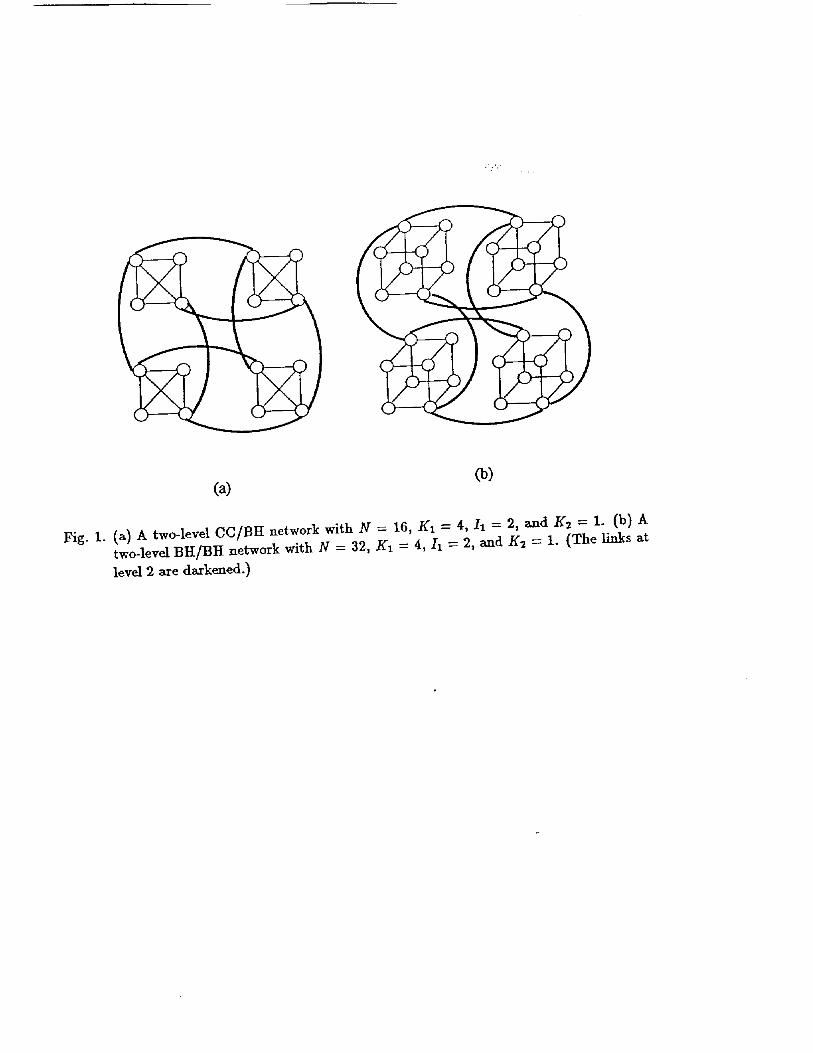
(a)Co)

Fig. 1. (a) A two-level CC/BH network with N = 16, Kt = 4, It = 2, and K2 -- 1. (b) Atwo-level BH/BH network with N = 32, Kt = 4, It -- 2, and Kx = 1. (The links at

level 2 are darkened.)

Fig. 2. (a) Outgoing messages via interface node (0000) in a subcluster (BIt) with 16 nodes.

(b) & (c) Incoming messages via interface nodes (0000) and (1111), respectively, in a

duster (BH) with 16 nodes.

15

10

)t/!

_""_---...._.,..._.....

'--"-*--_-.-., BH/BH

.... -----. CC/BH

I I I I0 -1 2 3 4 logll

Fig. 3. Diameter (Din) versus 11, with N-1024 and N/KI=16.

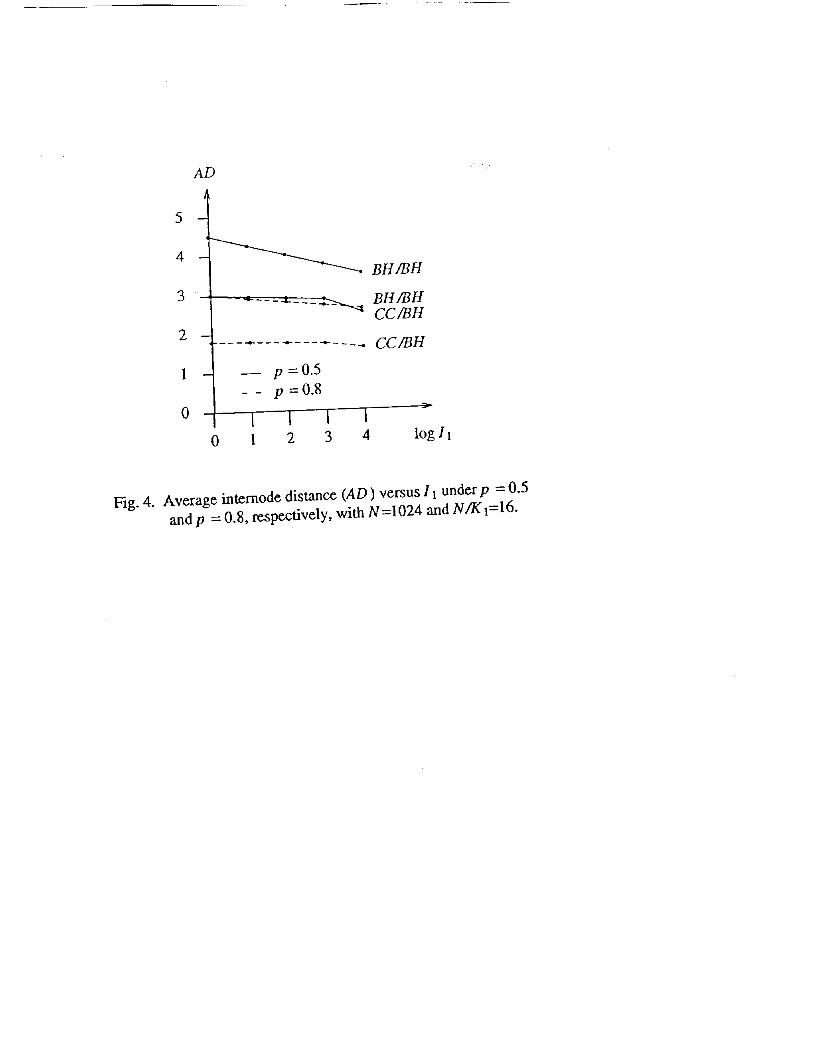
AD

4 -

.

2

1

0

BH/BH

- -,--- - _ .... _ BH/BHCC/BH

................. CC/BH

__ p=0.5

_- p=0.8

- I I I I0 1 2 3 4 log I l

Fig. 4. Average internode distance (AD) versus 11 under p = 0.5andp = 0.8, respectively, with N=I024 and N/KI=16-

_'D lrla x

i

10 -

8 _ * : TD_= TD_

- =

6 -

4

2

BH/BH(fix & even)

CC/BH

I } I I0 1 2 3 4 log I

(a) p = 0.5

TD_

4 t * : TD,,_ = TD,f_

3 ": TD_ = TD I'_?x

2

1

o I I I I I0 1 2 3 4

:x

log I I

(b) p =0.8

Fig. 5. The highesl traffic densily (TD_) versus 1_ under (a) p = 0.5and (b) p = 0.8, respectively, wilh N=1024 and N/Kt=16.

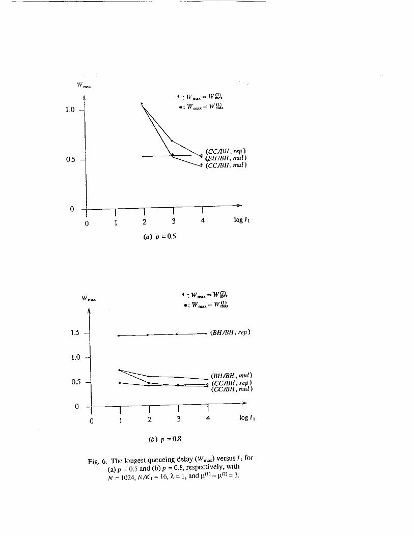
V( r_x

1.0 --

0.5

* : W_x = W_a¢

o I I I I0 1 2 3 4 log Ii

(a) p =0.5

W n_,_

1.5

1.0

0.5

(BH/BH, rep )

• _ (BH/BH, rout): _ (CC/BH, rep )

(CC/BH, mul)

I I I I1 2 3 4 log Ii

(b) p =0.8

Fig. 6. The longest queueing delay (W_) versus 11 for(a) p = 0.5 and (b) p = 0.8, respectively, withN = 1024, N/K1 = 16, _ = 1, and _(1)= t.t(2)= 3.

L*AD

30000.

25000-

20000,

15000-

10000-

5000

0

0

-- p =0.5

.... p =0.8

JCC/BH

BH/BH

CC/BHBH/BH

I I J I1 2 3 4 log 11

Fig. 7. L*AD versus 11 underp =0.5 andp =0.8,

respectively, with N=1024 and N/K1=16.

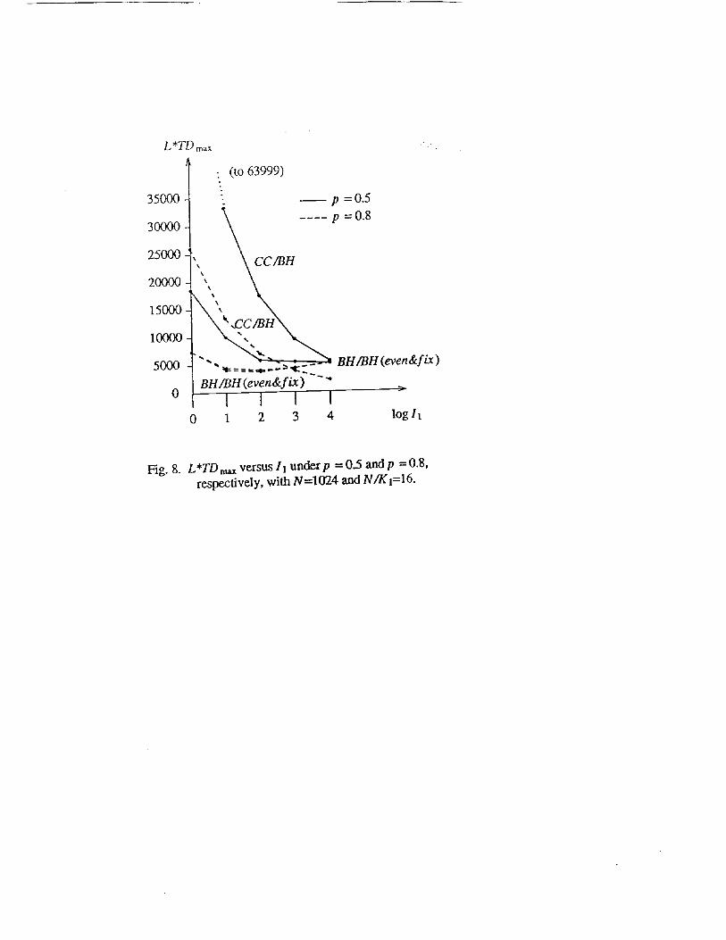
L*TDrn_x •

350OO

3O0OO

25000 -

20000

15O0O

10000

5OOO

0

: (to 63999)

_p =0.5.

.... p =0.8

", _C/BH

8HmH )BH/BH (even&fix ) -" >

I I I I0 1 2 3 4 log I t

Fig. 8. L*TDmax versus 11 underp =0.5 and p =0.8,respectively, with N=1024 and N/Ki=16.

L*Wr, u=

10000-

5000

0

p =0.5

- - - p = 0.8

".. (CC/BH)"- ..- - - - "(CC/BH)

,_._._(BH[BH)__ (BH/BH)

- I I I I0 1 2 3 4 log I t

Fig. 9. L*W,_.= versus It underp = 0.5 andp =0.8, respectively,with N=1024, N/KI=I6, X.--l, and l.t(1}= I.tO) = 3.