Advanced NMR Processing

Ulrich Günther

EuroLabCourse "Advanced Computing in NMR

Spectroscopy", Florence, Sept. 2001

Contents

1 Introduction 3

2 Wavelets 6

2.1 The Haar System . . . . . . . . . . . . . . . . . . . . . . . . . 6

2.2 Mallat’s Multiresolution Analysis . . . . . . . . . . . . . . . . 9

2.3 Thresholding . . . . .. . . . . . . . . . . . . . . . . . . . . . 14

2.4 Smoother Wavelet Bases . . . . . . . . . . . . . . . . . . . . . 15

2.5 Applications in NMR Spectroscopy . . . . . . . . . . . . . . . 17

2.5.1 WAVEWAT . . . . . . . . . . . . . . . . . . . . . . . . 17

2.5.2 Noise Suppression . . . . . . . . . . . . . . . . . . . . 21

2.5.3 Noise suppression in three-dimensional spectra .. . . . 22

3 SVD-based methods 24

3.1 SVD-based noise and signal suppression . . . .. . . . . . . . 24

3.2 Linear prediction . . . . . . . . . . . . . . . . . . . . . . . . . 28

4 Using NMRLab 31

2

1 Introduction

NMR processing has developed over many years since the introduction of Fourier

Transform (FT) -NMR spectroscopy by Richard Ernst. In FT-NMR spectroscopy

the response to a perturbation from equilibrium is recorded during a certain

amount of time. Because this response originates from the entire ensemble of

spins it is an interferogram containing many different frequencies. The basis

of all NMR processing is based on the fact that the interferogram can be de-

scribed as a superposition of decaying complex exponentials, a free induction

decay (FID). This signal is comparable to an acoustic signal , a high-frequency

sound originating from nuclear spins. For this reason many of the more recent

developments of acoustic signal processing are applicable to NMR signals.

Modern NMR spectroscopy benefits a lot from modern computational possi-

bilities. The measured FID is digitized and stored as a digital signal, i.e. a series

of complex data points.

NMR processing is used to convert this digital time-domain data into a fre-

quency spectrum. This basic task is usually achieved using a discrete Fourier

transform which provides a spectrum showing signal intensities versus frequency.

Discrete Fourier transforms (DFT) were revolutionized in 1965 by the publica-

tion of a fast algorithm by Cooley and Tukey requiringN log(N) rather thanN2

operations.

Experimental NMR-signals contain noise besides the signals of interest. Most

of this noise originates from the receiver circuitry. However, some of the noise is

also a consequence of subtle instabilities during long measurements. The Fourier

transform has the disadvantage that it convolutes noise with the spectrum. Sev-

eral approaches to reduce the noise in spectra are commonly used in modern

NMR processing. Most commonly the FID is multiplied with an apodization

function which damps noise towards the end of the FID. Apodization usually

broadens the original signal.

Many other steps are a part of regular NMR processing. Phase correction

3

1 Introduction

is used to obtain pure absorption mode spectra. The solvent signal is often

suppressed by removing on-resonance components from the FID. This can be

achieved using different algorithms. The most common is the subtraction of a

low-order polynomial which describes the slow variations in the FID. In pro-

tein NMR it is common to apply a convolution to the FID which also extracts

low-frequency components.

Baseline correction is often applied to the final spectrum. This is particu-

larly important for multi-dimensional NMR spectra which require a flat baseline

for visualization and for peak picking. Baseline correction requires two distinct

steps: differentiating between baseline and signal points and the calculation of a

suitable signal to subtract from the spectrum.

Several more advanced signal processing techniques were applied to NMR

spectroscopy. The most frequently used tool of this type is linear prediction, an

algorithm introduced by Tufts and Kumaresan in 1982 [16]. Delsuc first intro-

duced this tool for NMR processing [6]. Linear prediction is based on the fact

that signals are periodic during the course of an FID while noise is not. If it is

possible to determine coefficients which describe the intensity, decay and phase

of the signal components in a FID the noise contribution can be eliminated and

the course of the FID can be predicted beyond the duration during which the FID

was recorded. This technique uses singular value decomposition (SVD) to calcu-

late coefficients. Although it is computationally very demanding it is commonly

used in modern NMR processing.

Many other techniques have also been used to process NMR signals. Maxi-

mum entropy reconstruction is the most well-known algorithm which is available

in many NMR processing packages. MaxEnt uses a configurational entropy as

a regularization function which provides a measure for the approximation of the

calculated spectra to the experimental data. Bayesian analysis is a statistical

method to estimate the degree to which a hypothesis is confirmed by experi-

mental data. Bretthorst and Sibsi showed how Bayesian analysis can be used

to process NMR spectra. More recently continuous wavelet transforms (CWT)

were used to analyze NMR signals.

This course focuses on the use of discrete wavelet transforms (DWT) to re-

duce the noise level in NMR spectra and for suppression of the on-resonance

solvent signal. Wavelet algorithms are being rapidly introduced in many fields of

signal processing. The most common application of wavelets is probably image

and sound compression (e.g. in jpeg, mpeg and mp3 file formats). Smoothing

and noise suppression employing wavelet transforms was originally suggested

4

1 Introduction

by David Donoho [7, 8]. Other applications of wavelets include density esti-

mation, and nonparametric regression. In the course basic principles of wavelet

transforms will be presented.

All algorithms used in this course were implemented in NMRLab, a package

for NMR processing in MATLAB (The Mathworks). Most of the source code of

NMRLab is available. Although most of the routines were vectorized to maxi-

mize computational efficiency, a non-vectorized version is usually included as a

comment. For wavelet transforms routines from WAVELAB were used [1].

Christian Ludwig made significant contributions to the software used in this

course. The underlying work was supported by Prof. H. Rüterjans and the Large

Scale Facility at Frankfurt.

5

2 Wavelets

Wavelets are a topic of applied mathematics. The mathematical theory ofon-

delettes(wavelets) was developed by Yves Meyer almost 15 years ago. The

namewaveletoriginates from the the requirement for these functions to inte-

grate to zero, “waving” above and below thex-axis. Wavelets chop up data into

frequency components, and analyze each frequency component with a resolution

matched to its scale.

General interest in wavelets has grown substantially in the past 10 years be-

cause wavelets solve basic problems in signal processing such as data approxi-

mation (smoothing), noise reduction, data compression, time-frequency analysis

and image analysis. The availability of fast wavelet transform algorithms was

crucial for their success in signal processing. The application of wavelets to

smooth NMR signals has been inspired by David Donoho, one of the pioneers

of the field, who used an NMR spectrum as an example to illustrate potential

applications [7, 8]. In his book ’NMR data processing’ J. Hoch describes emerg-

ing methods in NMR data processing and shows an example for smoothing by

wavelets following the ideas of Donoho [14]. More recent publications describe

the use of wavelets in NMR processing [12, 11].

It is the aim of this course to introduce basic principles of wavelet analysis

and potential applications to NMR researchers. For more advanced reading we

refer to many excellent text books [17, 5, 13] and introductory texts [18, 21, 15,

9, 19].

2.1 The Haar System

There are many types of wavelets. The most simple wavelet is the Haar wavelet

introduced in an appendix of the thesis of A. Haar in 1909. The Haar function is

6

2 Wavelets

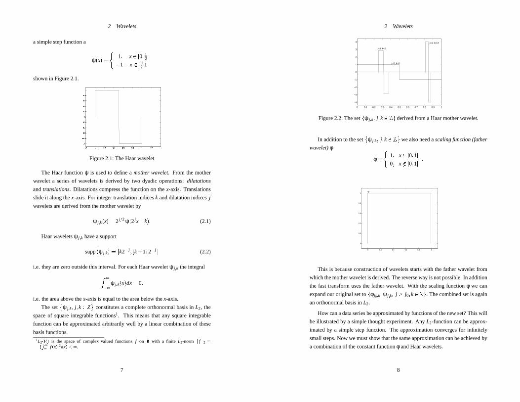
a simple step function a

ψ(x) =(

1; x2 [0; 12[

�1; x2 [ 12;1[

shown in Figure 2.1.

Figure 2.1: The Haar wavelet

The Haar functionψ is used to define amother wavelet. From the mother

wavelet a series of wavelets is derived by two dyadic operations:dilatations

andtranslations. Dilatations compress the function on thex-axis. Translations

slide it along thex-axis. For integer translation indicesk and dilatation indicesj

wavelets are derived from the mother wavelet by

ψ j ;k(x) = 2 j=2 ψ(2 j x�k): (2.1)

Haar waveletsψ j ;k have a support

supp

�

ψ j ;k

�=

�

k2� j ;(k+1)2� j� (2.2)

i.e. they are zero outside this interval. For each Haar waveletψ j ;k the integral

Z ∞

�∞ψ j ;k(x)dx= 0:

i.e. the area above thex-axis is equal to the area below thex-axis.

The set

�

ψ j ;k; j;k2 Z

constitutes a complete orthonormal basis inL2, the

space of square integrable functions1. This means that any square integrable

function can be approximated arbitrarily well by a linear combination of these

basis functions.1L2(R) is the space of complex valued functionsf on R with a finite L2-norm jj f jj2 =�R ∞

∞ j f (x)j2dx

�<∞.

7

2 Wavelets

0 0.1 0.2 0.3 0.4 0.5 0.6 0.7 0.8 0.9 1

−4

−3

−2

−1

0

1

2

3

4

j=3, k=2

j=0, k=0

j=4, k=13

Figure 2.2: The setfψ j ;k; j;k2 Zg derived from a Haar mother wavelet.

In addition to the set

�ψ j ;k; j;k2 Zwe also need ascaling function (father

wavelet)φ

φ =(

1; x2 [0;1[

0; x =2 [0;1[:

0 0.2 0.4 0.6 0.8 1

0

0.2

0.4

0.6

0.8

1φ

This is because construction of wavelets starts with the father wavelet from

which the mother wavelet is derived. The reverse way is not possible. In addition

the fast transform uses the father wavelet. With the scaling functionφ we can

expand our original set tofφ j0;k; ψ j ;k; j � j0;k2 Zg. The combined set is again

an orthonormal basis inL2.

How can a data series be approximated by functions of the new set? This will

be illustrated by a simple thought experiment. AnyL2-function can be approx-

imated by a simple step function. The approximation converges for infinitely

small steps. Now we must show that the same approximation can be achieved by

a combination of the constant functionφ and Haar wavelets.

8

2 Wavelets

Any square integrable function2 f (x) can be described by

f (x) = c00φ(x)+

n�1

∑j=0

2 j�1

∑k=0

cj ;kψ j ;k(x) ; (2.3)

wherecj ;k are wavelet coefficients,ψ j ;k are wavelets derived from a mother

waveletψ andφ is a scaling function (father wavelet), in the case of the Haar

wavelet transform it is unity on the interval[0;1[. Using equation 2.4 a function

f can be decomposed into a linear combination of waveletsψ j ;k. The same is

true for a data series which can be described by a functionf (x).

Wavelet transforms share many properties with Fourier transforms. The al-

gorithm to determine wavelet coefficients is even faster than FFT. While the fast

Fourier transform algorithm by Cooley and Tukey requiresN log(N) operations,

the dyadic wavelet transform gets along with onlyN operations.

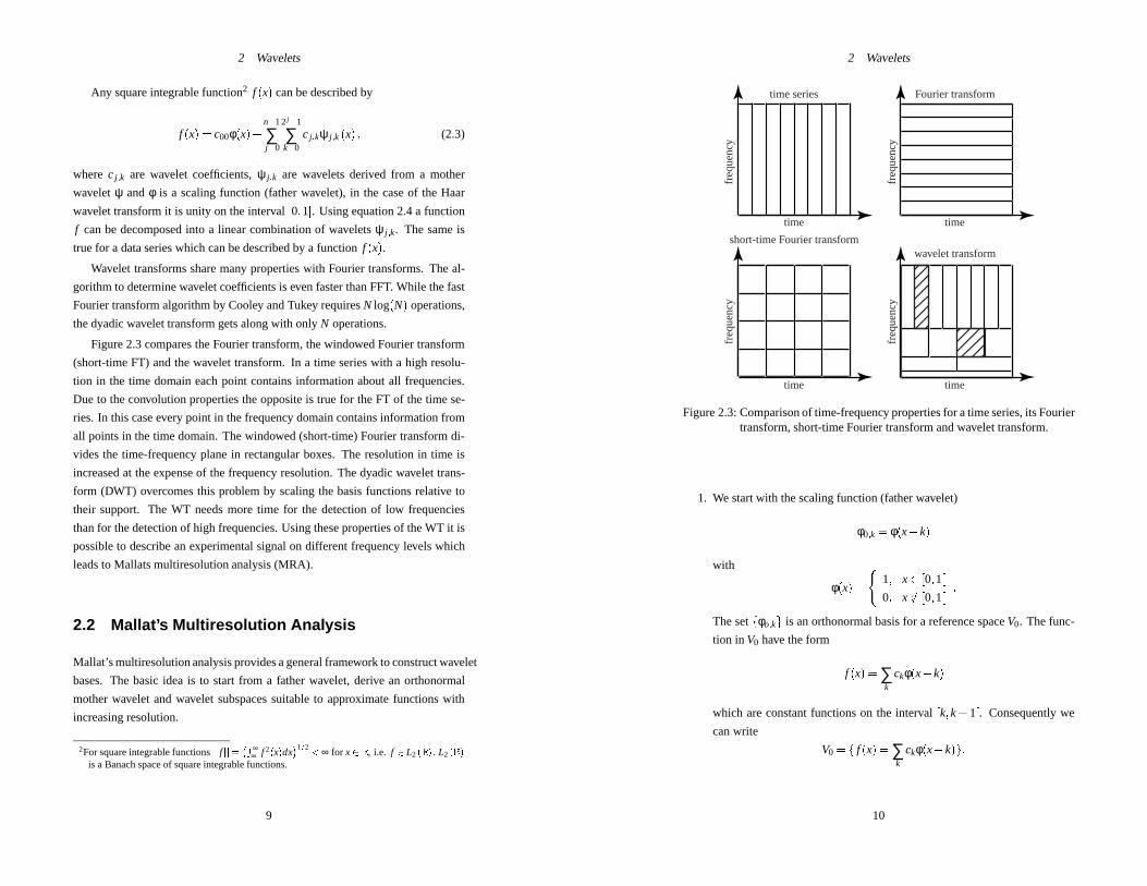
Figure 2.3 compares the Fourier transform, the windowed Fourier transform

(short-time FT) and the wavelet transform. In a time series with a high resolu-

tion in the time domain each point contains information about all frequencies.

Due to the convolution properties the opposite is true for the FT of the time se-

ries. In this case every point in the frequency domain contains information from

all points in the time domain. The windowed (short-time) Fourier transform di-

vides the time-frequency plane in rectangular boxes. The resolution in time is

increased at the expense of the frequency resolution. The dyadic wavelet trans-

form (DWT) overcomes this problem by scaling the basis functions relative to

their support. The WT needs more time for the detection of low frequencies

than for the detection of high frequencies. Using these properties of the WT it is

possible to describe an experimental signal on different frequency levels which

leads to Mallats multiresolution analysis (MRA).

2.2 Mallat’s Multiresolution Analysis

Mallat’s multiresolution analysis provides a general framework to construct wavelet

bases. The basic idea is to start from a father wavelet, derive an orthonormal

mother wavelet and wavelet subspaces suitable to approximate functions with

increasing resolution.

2For square integrable functionsjj f jj=�R ∞

∞ f 2(x)dx

�1=2

< ∞ for x2 R, i.e. f 2 L2 (R). L2 (R)

is a Banach space of square integrable functions.

9

2 Wavelets

time time

time time

freq

uenc

y

freq

uenc

y

freq

uenc

y

freq

uenc

y

time series Fourier transform

short-time Fourier transformwavelet transform

Figure 2.3: Comparison of time-frequency properties for a time series, its Fouriertransform, short-time Fourier transform and wavelet transform.

1. We start with the scaling function (father wavelet)

φ0;k = φ(x�k)

with

φ(x) =(

1; x2 [0;1[

0; x =2 [0;1[:

The setfφo;kg is an orthonormal basis for a reference spaceV0. The func-

tion in V0 have the form

f (x) = ∑k

ckφ(x�k)

which are constant functions on the interval[k;k+ 1[. Consequently we

can write

V0 = f f (x) = ∑k

ckφ(x�k)g:

10

2 Wavelets

2. Starting fromV0 we define linear spaces

V1 = fh(x) = f (2x) : f 2V0g

...

Vj = fh(x) = f (2 j x) : f 2V0g

V1 contains all functions constant on[k2;

k+12 [. The setfφ1;kg is an orthonor-

mal basis inV1with φ1;k(x) =p

2φ(2x�k).

Analogously, the basis functions ofVj areφ j ;k = 2 j=2φ(2 jx�k).

φ generates a sequence of spacesfVj ; j 2 Zgwhich are nested:

V0 �V1 � : : :�Vj � : : :

Vj �Vj+1; j 2 Z:

If in addition every square integrable function can be approximated by

functions in [

j�0

Vj

thanfVj ; j 2 Zg is a MRA3.

3S

j�0Vj is dense inL2(R)

11

2 Wavelets

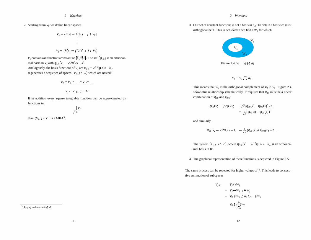
3. Our set of constant functions is not a basis inL2. To obtain a basis we must

orthogonalize it. This is achieved if we find aW0 for which

V0

V1

W0

Figure 2.4:V1 =V0L

W0:

V1 =V0

M

W0:

This means thatW0 is the orthogonal complement ofV0 in V1. Figure 2.4

shows this relationship schematically. It requires thatφ1k must be a linear

combination ofφ0k andψ0k:

φ10(x) =p

2φ(2x) =p

2fφ00(x)�ψ00(x)g=2

= 1p

2

fφ00(x)�ψ00(x)g

and similarly

φ11(x) =p

2φ(2x�1) = 1p

2

fφ00(x)+ψ00(x)g=2 :

The systemfψ j ;k;k2 Zg, whereψ j ;k(x) = 2 j=2ψ(2 j x�k), is an orthonor-

mal basis inWj .

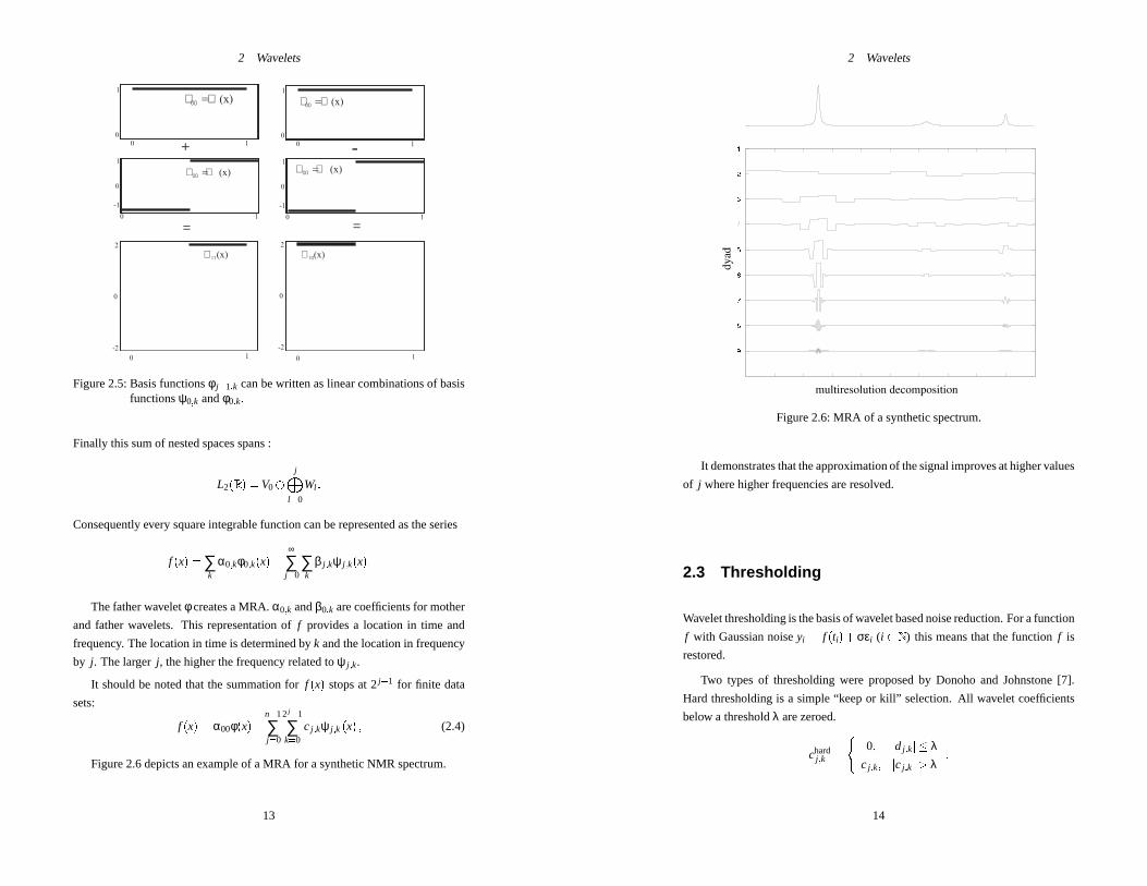
4. The graphical representation of these functions is depicted in Figure 2.5.

The same process can be repeated for higher values ofj. This leads to consecu-

tive summation of subspaces

Vj+1 = Vj �Wj

= Vj �Wj�1�Wj

= V0�W0�W1� :::�Wj

= V0�

jM

l=0

Wl

12

2 Wavelets

==

-+1 1

1 1

1

2 2

-2 -2

1

1

1 1

1

-1 -1

0

0 0

0

0 0

0

0 0

0

0 0

f f00

= (x)

F11

(x) F10

(x)

y y00

= (x) y y00

= (x)

f f00

= (x)

Figure 2.5: Basis functionsφ j+1;k can be written as linear combinations of basisfunctionsψ0;k andφ0;k.

Finally this sum of nested spaces spans :

L2(R) =V0�

jM

l=0

Wl :

Consequently every square integrable function can be represented as the series

f (x) = ∑k

α0;kφ0;k(x)+

∞

∑j=0

∑k

β j ;kψ j ;k(x):

The father waveletφ creates a MRA.α0;k andβ0;k are coefficients for mother

and father wavelets. This representation off provides a location in time and

frequency. The location in time is determined byk and the location in frequency

by j. The largerj, the higher the frequency related toψ j ;k.

It should be noted that the summation forf (x) stops at 2j�1 for finite data

sets:

f (x) = α00φ(x)+

n�1

∑j=0

2 j�1

∑k=0

cj ;kψ j ;k(x) ; (2.4)

Figure 2.6 depicts an example of a MRA for a synthetic NMR spectrum.

13

2 Wavelets

Figure 2.6: MRA of a synthetic spectrum.

It demonstrates that the approximation of the signal improves at higher values

of j where higher frequencies are resolved.

2.3 Thresholding

Wavelet thresholding is the basis of wavelet based noise reduction. For a function

f with Gaussian noiseyi = f (ti)+σεi (i 2 N) this means that the functionf is

restored.

Two types of thresholding were proposed by Donoho and Johnstone [7].

Hard thresholding is a simple “keep or kill” selection. All wavelet coefficients

below a thresholdλ are zeroed.

chardj ;k =

(

0; jdj ;kj � λcj ;k; jcj ;kj> λ

:

14

2 Wavelets

Soft thresholding shrinks the coefficients towards zero:

csoftj ;k =

8><>:

cj ;k�λ; cj ;k > λ0; jcj ;kj � λ

cj ;k+λ; cj ;k <�λ

:

The two shrinkage methods are displayed in Figure 2.7. The most important step

is now a proper choice of the thresholdλ. Donoho and Johnstone showed that

a universal thresholdλ = σ

p

2logn=p

n wheren is the sample size andσ the

scale of the noise on a standard deviation scale4.

Figure 2.7: Hard and soft thresholding.

The overall procedure of noise suppression consists of a wavelet transform

(WT) which yields the wavelet coefficientscj ;k, thresholding of these coefficients

followed by an inverse wavelet transform (IWT) which restores the original spec-

trum.

2.4 Smoother Wavelet Bases

Although the Haar wavelet is convenient to describe the basics of wavelet trans-

forms it is not suitable for most wavelet applications because too many coef-

ficients are required to approximate a signal. The description of the design of

smoother wavelet bases is far beyond the scope of this script. Wavelet bases

must form an orthonormal basis forL2(R). Wavelets with good smoothing prop-

erties are designed to minimize the wavelet coefficients for smooth functions.

The number of such constraints applied during the design of wavelets determines

the number of vanishing moments. Wavelets of the Daubechies family shown in

Figure 2.8 also have compact support which is important for noise reduction.

Daubechies wavelets have vanishing moments for mother but not for father

wavelets and are fairly asymmetric. Coiflets have additional vanishing moments

for father wavelets. Symmlets are as close to symmetry as possible.

Basic properties of wavelets with compact support:

4σ =

median(jcJ�1;k�median(cJ�1;k)j)

0:6745

15

2 Wavelets

Figure 2.8: Types of wavelets from left to right: Daubechies (4), Coiflet (5) andSymmlet (8).

� Daubechies’ wavelets:

suppφ � [0;2N�1]

suppψ � [�N+1;N]R

xl ψ(x)dx= 0; l = 0; :::;N�1

For the D4 Daubechies wavelet:

Rψ(x)dx= 0,

R

xψ(x)dx= 0.

Not symmetric.

� Coiflets

N = 2K

suppφ � [�2K;4K�1]

suppψ � [�4K+1;2K]Rxl φ(x)dx= 0; l = 0; :::;N�1Rxl ψ(x)dx= 0; l = 0; :::;N�1

Coiflets are not symmetric.� Symmlets

suppφ � [0;2N�1]

suppψ � [�N+1;N]R

xl ψ(x)dx= 0; l = 0; :::;N�1

� Symmlets are not symmetric.

16

2 Wavelets

2.5 Applications in NMR Spectroscopy

MRA and wavelet shrinkage have useful applications in NMR spectroscopy.

MRA of the FID can be used to remove slow frequencies from the FID, i.e. to

remove on-resonance components. Wavelet shrinkage has been used to denoise

one- and multi-dimensional NMR-spectra.

2.5.1 WAVEWAT

Figure 2.9 shows a multiresolution decomposition of a FID. The high- and low-

frequency components are nicely separated.

0 0.1 0.2 0.3 0.4 0.5 0.6 0.7 0.8 0.9 1t

Dya

d

Multiresolution Decomposition

100 200 300 400 500 600 700 800 900 1000

J=7 Reconstruction.

Figure 2.9: Top: Multiresolution plot of a FID from a15N-HSQC spectrumrecorded at 500 MHz using a 1.2 mM protein sample. Bottom: Orig-inal FID and FID recovered from the MRA (gray) shown in Figure 1using only using levels withJ� 7.

Edge effects seen in Figure 2.9 are minimized when mirror reflections of the

FID are used for the MRA. A basic limitation is the fact that the number of dyadic

levels is limited by 2J = N because the number of dyadic levels determines the

width of the filter. A sufficiently large number of data points for a reasonably

narrow filter width can be obtained by repeated zero filling.

An example of a DWT water suppression is illustrated in Figure 2.10. The

signal originated from a15N-HSQC spectrum of a SH2 domain. The low in-

tensity signal close to water was added synthetically to the experimental FID to

17

2 Wavelets

0 500 1000 1500 2000 2500 3000 3500 4000 4500−500

0

500

1000

1500

2000

2500

3000

demonstrate the effect of the filter. It can hardly be detected in Figure 2.10A

underneath the strong water resonance which is not in phase with the rest of the

spectrum. In Figure 2.10B the WAVEWAT-filtered spectrum (zero filling once,

ZF = 2; reconstruction using levels� 7, J = 7) is shown. Peak shapes and in-

tensities are recovered perfectly. For comparison the effect of a convolution filter

employing a 32 points Gaussian apodization function is shown (Figure 2.10C).

This algorithm was originally proposed by Marionet al. [4]. Figure 2.11 demon-

strates the principles of this filter.

Here the signal close to water is barely recovered and significantly distorted.

Both the WAVEWAT and the convolution filter do not distort off-resonance peaks

in the spectrum.

Noise levels were calculated for all columns of a two-dimensional HSQC

spectrum after convolution water suppression and WAVEWAT water suppres-

sion. For convolution water suppression the noise level is reduced over an area

of at least 80 points close to the water signal (Figure 2.12A). For WAVEWAT the

area in which signals are distorted is much narrower and the edge of the filter is

sharper. This is demonstrated in Figure 2.12B where a symmlet wavelet with 8

vanishing moments (Symmlet(8)) has been used after zero filling to 1024 points

andJ = 7. In Figure 4C the same wavelet is used after zero filling to 1024 points

usingJ = 9. In Figure 4B the area in which signals are suppressed is narrower

and the edges of the water signal becomes visible. In this case signals close to

water will be recovered without distortion of signal intensities. Although ap-

proximately 20 points close to the water resonance were eliminated in Figure

2.12C, the spectral area which is affected by the filter is much smaller than that

18

2 Wavelets

−500 −400 −300 −200 −100 0 100

A

−500 −400 −300 −200 −100 0 100

B

−500 −400 −300 −200 −100 0 100

C

Figure 2.10: Spectrum obtained from the FID shown in Figure 2 after Fouriertransformation. The small signal close to water was added synthet-ically to the experimental FID. A: Fourier transformed spectrumwithout prior water suppression. B: WAVEWAT was applied ap-plied to the FID prior to Fourier transformation; the signal was zero-filled to 2048 points prior to MRA; the signal was recovered afterrejecting 7 levels as shown in Figure 1; a symmlet (8) wavelet wasused for the wavelet transform. C: water suppression was achievedby a convolution of the FID with a 32-point Gaussian window.

in the case of a convolution filter.

19

2 Wavelets

Figure 2.11: Convolution filter for noise suppression.

0 100 200 300 400 500 600

nois

e

0 100 200 300 400 500 600

nois

e

0 100 200 300 400 500 600

nois

e

A

B

C

Figure 2.12: Noise levels calculated for the incremented dimension. A: after wa-ter suppression using time-domain convolution ; B: after water sup-pression using WAVEWAT after zero-filling to 1024 points usinglevels� 7; C: after water suppression using WAVEWAT after zero-filling to 1024 points using levels� 9.

20

2 Wavelets

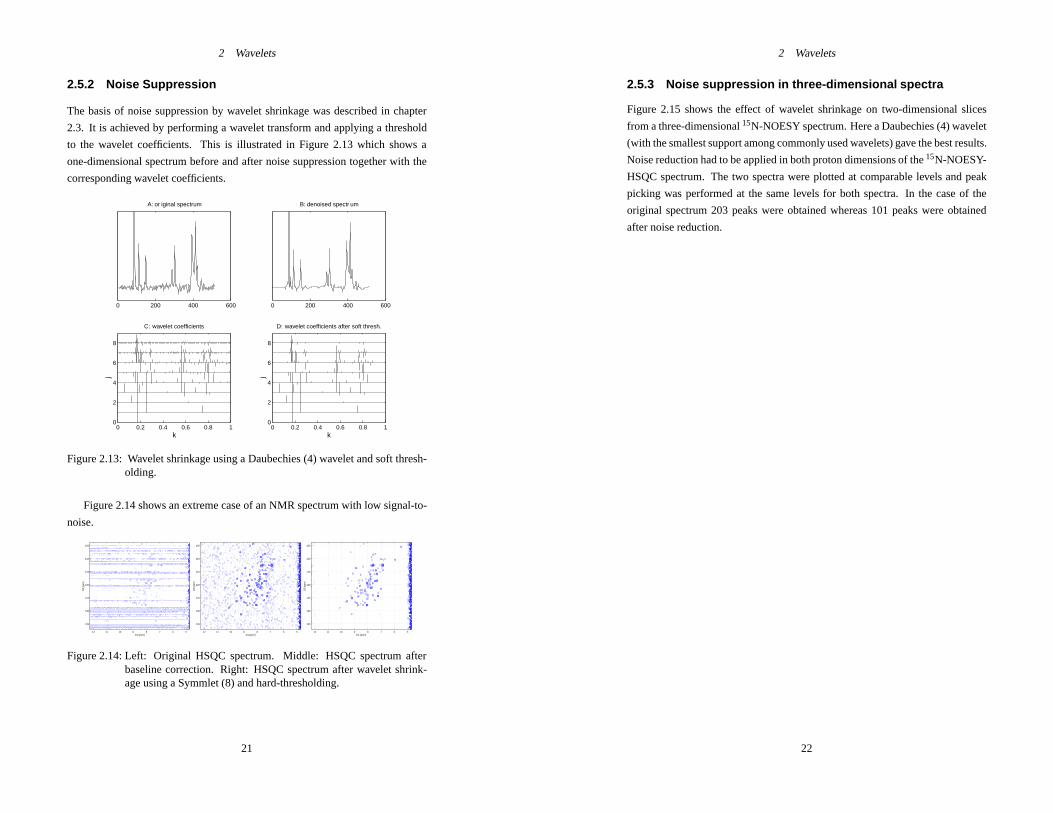
2.5.2 Noise Suppression

The basis of noise suppression by wavelet shrinkage was described in chapter

2.3. It is achieved by performing a wavelet transform and applying a threshold

to the wavelet coefficients. This is illustrated in Figure 2.13 which shows a

one-dimensional spectrum before and after noise suppression together with the

corresponding wavelet coefficients.

0 0.2 0.4 0.6 0.8 10

2

4

6

8

k

j

C: wavelet coefficients

0 200 400 600

A: or iginal spectrum

0 0.2 0.4 0.6 0.8 10

2

4

6

8

k

j

D: wavelet coefficients after soft thresh.

0 200 400 600

B: denoised spectr um

Figure 2.13: Wavelet shrinkage using a Daubechies (4) wavelet and soft thresh-olding.

Figure 2.14 shows an extreme case of an NMR spectrum with low signal-to-

noise.

56789101112

105

110

115

120

125

130

135

D1 [ppm]

D2

[ppm

]

56789101112

105

110

115

120

125

130

135

D1 [ppm]

D2

[ppm

]

56789101112

105

110

115

120

125

130

135

D1 [ppm]

D2

[ppm

]

Figure 2.14: Left: Original HSQC spectrum. Middle: HSQC spectrum afterbaseline correction. Right: HSQC spectrum after wavelet shrink-age using a Symmlet (8) and hard-thresholding.

21

2 Wavelets

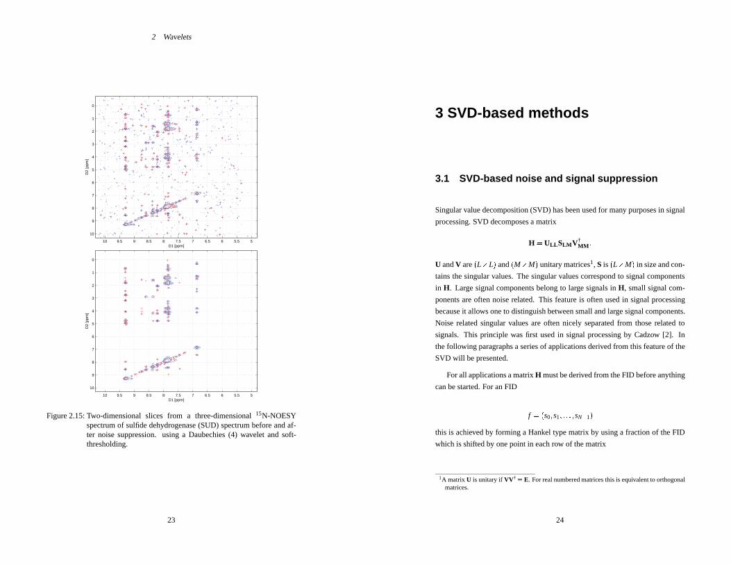
2.5.3 Noise suppression in three-dimensional spectra

Figure 2.15 shows the effect of wavelet shrinkage on two-dimensional slices

from a three-dimensional15N-NOESY spectrum. Here a Daubechies (4) wavelet

(with the smallest support among commonly used wavelets) gave the best results.

Noise reduction had to be applied in both proton dimensions of the15N-NOESY-

HSQC spectrum. The two spectra were plotted at comparable levels and peak

picking was performed at the same levels for both spectra. In the case of the

original spectrum 203 peaks were obtained whereas 101 peaks were obtained

after noise reduction.

22

2 Wavelets

55.566.577.588.599.510

0

1

2

3

4

5

6

7

8

9

10

D1 [ppm]

D2

[ppm

]

55.566.577.588.599.510

0

1

2

3

4

5

6

7

8

9

10

D1 [ppm]

D2

[ppm

]

Figure 2.15: Two-dimensional slices from a three-dimensional15N-NOESYspectrum of sulfide dehydrogenase (SUD) spectrum before and af-ter noise suppression. using a Daubechies (4) wavelet and soft-thresholding.

23

3 SVD-based methods

3.1 SVD-based noise and signal suppression

Singular value decomposition (SVD) has been used for many purposes in signal

processing. SVD decomposes a matrix

H = ULL SLM V†MM :

U andV are(L�L) and(M�M) unitary matrices1, S is (L�M) in size and con-

tains the singular values. The singular values correspond to signal components

in H. Large signal components belong to large signals inH, small signal com-

ponents are often noise related. This feature is often used in signal processing

because it allows one to distinguish between small and large signal components.

Noise related singular values are often nicely separated from those related to

signals. This principle was first used in signal processing by Cadzow [2]. In

the following paragraphs a series of applications derived from this feature of the

SVD will be presented.

For all applications a matrixH must be derived from the FID before anything

can be started. For an FID

f = (s0;s1; : : : ;sN�1)

this is achieved by forming a Hankel type matrix by using a fraction of the FID

which is shifted by one point in each row of the matrix

1A matrix U is unitary ifVV† = E. For real numbered matrices this is equivalent to orthogonalmatrices.

24

3 SVD-based methods

H =0

BBBB@

s0 s1 s2 � � � sM�1

s1 s2 s3 � � � sM...

...... � � � ...

sL�1 sL sL+1 � � � sN�1

1CCCCA :

For a FID which does not contain any noise the rank of this matrix is equiv-

alent to the number of signals in the FID. However, if the signal contains noise

the rank will be full (M).

The SVD picks up periodicities in the FID. Periodic components in the FID

will be represented by singular values. On the diagonal ofS the singular values

are sorted by size. This makes it very easy to select signal components. An

example is presented in Figure 3.1. The noise test signal contains three distinct

signals which are represented by three distinct singular values. In principle it

is straightforward to use this procedure to suppress noise. If all singular values

below the blue line are set to zero and the FID is restored fromH a noise-free

signal is obtained. The difficulty is always to find the noise level.

0 50 100 150 200 250 300−5

0

5

10

15

20

25

0 10 20 30 40 50 60 70 80 900

2

4

6

8

10

12

14

16

18

20

Abbildung 3.1: Left: NMR spectrum with three signals. Right: singular valuessorted by size. Blue line: noise level.

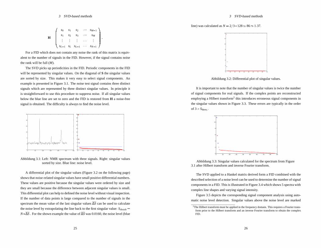
A differential plot of the singular values (Figure 3.2 on the following page)

shows that noise-related singular values have small positive differential numbers.

These values are positive because the singular values were ordered by size and

they are small because the difference between adjacent singular values is small.

This differential plot can help to defined the noise level without visual inspection.

If the number of data points is large compared to the number of signals in the

spectrum the mean value of the last singular values∆Scan be used to calculate

the noise level by extrapolating the line back to the first singular value:Sthresh=

N�∆S. For the shown example the value of∆Swas 0.0160, the noise level (blue

25

3 SVD-based methods

line) was calculated asN = 2=3�128' 86� 1:37.

0 10 20 30 40 50 60 70 80 900

2

4

6

8

10

12

14

Abbildung 3.2: Differential plot of singular values.

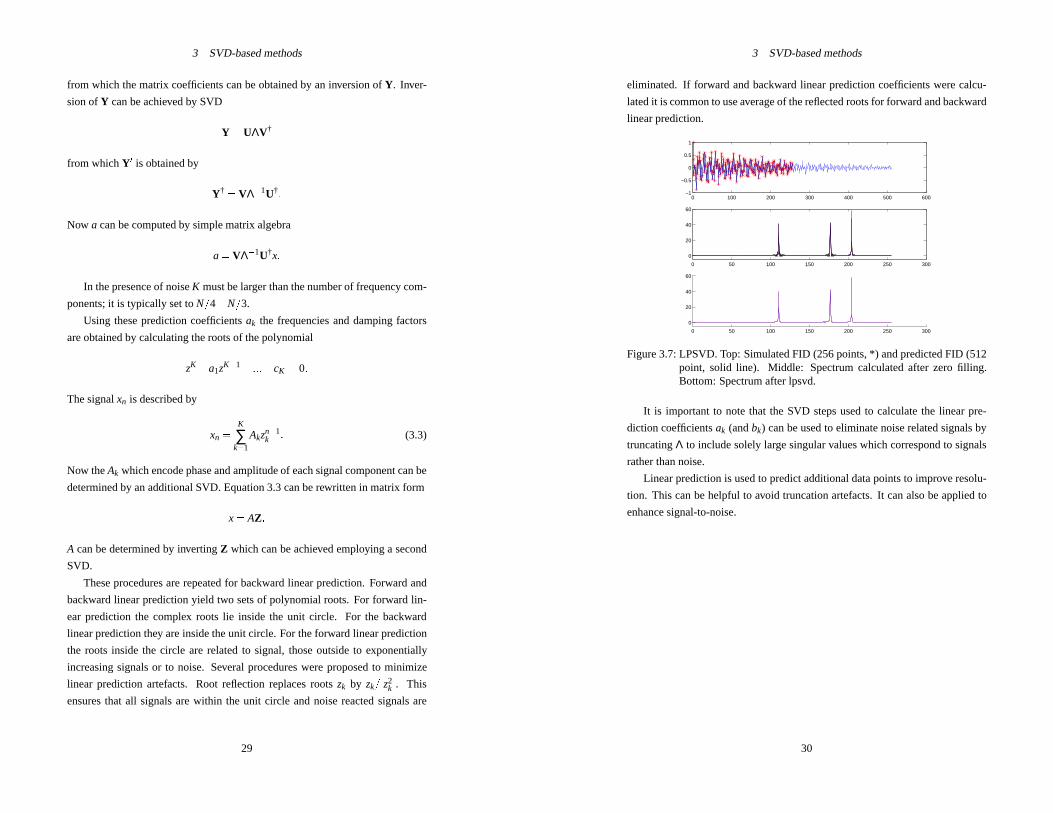
It is important to note that the number of singular values is twice the number

of signal components for real signals. If the complex points are reconstructed

employing a Hilbert transform2 this introduces erroneous signal components in

the singular values shown in Figure 3.3. These errors are typically in the order

of 3�Sthres:.

0 10 20 30 40 50 60 70 80 900

2

4

6

8

10

12

Abbildung 3.3: Singular values calculated for the spectrum from Figure3.1 after Hilbert transform and inverse Fourier transform.

The SVD applied to a Hankel matrix derived form a FID combined with the

described selection of a noise level can be used to determine the number of signal

components in a FID. This is illustrated in Figure 3.4 which shows 5 spectra with

complex line shapes and varying signal intensity.

Figure 3.5 depicts the corresponding signal component analysis using auto-

matic noise level detection. Singular values above the noise level are marked

2The Hilbert transform must be applied in the frequency domain. This requires a Fourier trans-form prior to the Hilbert transform and an inverse Fourier transform to obtain the complexFID.

26

3 SVD-based methods

0 5 10 15 20 25 30−0.2

0

0.2

0.4

0.6

0.8

1

1.2

1.4

1.6

1.8

283K

293K

305K

308K

311K

Abbildung 3.4: Test signals for signal component analysis.

by an extra circle. The results are in good agreement with the number of signal

components seen by visual inspection.

1 2 3 4 5 6 70.01

0.02

0.03

0.04

0.05

0.06

0.07

0.08

0.09

0.1

0.11

283K

1 2 3 4 5 6 70

0.02

0.04

0.06

0.08

0.1

0.12

0.14

0.16

0.18

293K

1 2 3 4 5 6 70

0.05

0.1

0.15

0.2

0.25

0.3

0.35

0.4

0.45

305K

1 2 3 4 5 6 70

0.1

0.2

0.3

0.4

0.5

0.6

0.7

308K

1 2 3 4 5 6 70

0.1

0.2

0.3

0.4

0.5

0.6

0.7

0.8

311K

Abbildung 3.5: Singular values for the 5 spectra shown in Figure 3.4.

The same principle was used by Cadzow to suppress the noise level in signals

[2]. The principle is shown in Figure 3.6a. By dropping the noise related singular

values an almost noise-free spectrum is obtained.

The procedure can also be used in the other direction to suppress signals.

This is demonstrated in Figure 3.6b where the largest signal component was ze-

roed. This eliminated one signal in the corresponding spectrum. For equally

sized signals the choice of the peak which will be eliminated will be random.

However, if the largest signal is to be eliminated the method is very stable. This

algorithm has been used in NMR processing to eliminate large diagonal peaks

27

3 SVD-based methods

0 2 0 4 0 6 0 8 0 1 0 0 1 2 0 1 4 0

0 5 1 0 1 5 2 0 2 5 3 0 3 5 4 0 4 5

s i g n a l s = 3

2 0 4 0 6 0 8 0 1 0 0 1 2 0 1 4 0

0 5 1 0 1 5 2 0 2 5 3 0 3 5 4 0 4 5

s i g n a l s = - 1

P u n k t e P u n k t e

P u n k t e P u n k t e

a b

c d

Abbildung 3.6: Cadzow noise suppression and signal suppression.

in NOESY spectra [22]. It is almost routinely used to suppress the water sig-

nal in in vivo MRS [20, 23]. Unfortunately this algorithm can not be used for

high-resolution NMR-spectra and for large multi-dimensional spectra because

the SVD is aO((L�M)2M) process.

3.2 Linear prediction

Linear prediction has in principle nothing to do with SVD. However, SVD is

frequently used to determine LP coefficients. This version of linear prediction is

called LP-SVD. The LP-SVD algorithm was originally described by Kumaresan

and Tufts [16] and modified by Porat and Friedlander.

The forward linear prediction model assumes that a data point can be de-

scribed by a linear combination ofK preceding points

xn =

K

∑k=1

akxn�k; (3.1)

the backward linear prediction model by a linear combination of theK fol-

lowing points:

xn =

K

∑k=1

bkxn+k: (3.2)

Equation 3.1 can be written in matrix form as

x= a �Y

28

3 SVD-based methods

from which the matrix coefficients can be obtained by an inversion ofY. Inver-

sion ofY can be achieved by SVD

Y = UΛV†

from whichY0 is obtained by

Y† = VΛ�1U†:

Now a can be computed by simple matrix algebra

a= VΛ�1U†x:

In the presence of noiseK must be larger than the number of frequency com-

ponents; it is typically set toN=4�N=3.

Using these prediction coefficientsak the frequencies and damping factors

are obtained by calculating the roots of the polynomial

zK �a1zK�1� :::�cK = 0:

The signalxn is described by

xn =

K

∑k=1

Akzn�1k : (3.3)

Now theAk which encode phase and amplitude of each signal component can be

determined by an additional SVD. Equation 3.3 can be rewritten in matrix form

x= AZ:

A can be determined by invertingZ which can be achieved employing a second

SVD.

These procedures are repeated for backward linear prediction. Forward and

backward linear prediction yield two sets of polynomial roots. For forward lin-

ear prediction the complex roots lie inside the unit circle. For the backward

linear prediction they are inside the unit circle. For the forward linear prediction

the roots inside the circle are related to signal, those outside to exponentially

increasing signals or to noise. Several procedures were proposed to minimize

linear prediction artefacts. Root reflection replaces rootszk by zk=jz2kj. This

ensures that all signals are within the unit circle and noise reacted signals are

29

3 SVD-based methods

eliminated. If forward and backward linear prediction coefficients were calcu-

lated it is common to use average of the reflected roots for forward and backward

linear prediction.

0 100 200 300 400 500 600−1

−0.5

0

0.5

1

0 50 100 150 200 250 300

0

20

40

60

0 50 100 150 200 250 300

0

20

40

60

Figure 3.7: LPSVD. Top: Simulated FID (256 points, *) and predicted FID (512point, solid line). Middle: Spectrum calculated after zero filling.Bottom: Spectrum after lpsvd.

It is important to note that the SVD steps used to calculate the linear pre-

diction coefficientsak (andbk) can be used to eliminate noise related signals by

truncatingΛ to include solely large singular values which correspond to signals

rather than noise.

Linear prediction is used to predict additional data points to improve resolu-

tion. This can be helpful to avoid truncation artefacts. It can also be applied to

enhance signal-to-noise.

30

4 Using NMRLab

The algorithms described in this course were implemented in NMRLab [10].

NMRLab uses MATLAB (The Mathworks). Here some of the most basic tools

and data structures in NMRLab are described.

NMRPAR is initialized as a global structure bynmrlab.m and holds all basic

parameters required to run NMRLAB. The fields of NMRPAR define availability

of RAM, computer type (detected bynmrlab.m ) and other parameters.

The NMRDAT structure

NMRDAT is a global structure which is another set up by thenmrlab.m script

usually executed fromSTARTUP. Some fields can be edited, saved and restored

usingBROWSEbut NMRDAT it is also manually readable on the MATLAB com-

mand line. Table 4.1 lists the field names in NMRDAT.

Table 4.1: NMRDAT structureNMRDAT field name

NAME Dataset name. Used for saving substructure to disk.SER Converted SER file.MAT Processed data matrix.ACQUS Acquisition parameters (3D).PROC Processing parameters (3D).DISP Display parameters.

NAMEis a string describing the name of the.mat file when data is saved to

disk with the browse command. This is the only use ofNAME. It has no influence

on the name of the data after it is retrieved because a data set will always become

an element in theNMRDATstructure.

SERis simply an array for FIDs in the order they were recorded. The fast (t2)

dimension is in columns.MATis the processed data matrix with dimension 1 in

rows. This is not consequent but it saves time when data is displayed because the

contour command logically plots matrix rows as rows, the way we usually look

31

4 Using NMRLab

at two-dimensional NMR data.MATis set to ’-1’ when a matrix is saved to disk

and deleted from RAM.

ACQUScontains the acquisition parameters which were read from the BRUKER

acqus, acqu2s and acqu3s files with the readacqus command. It is itself a two

or three dimensional array which contains the information for the three spectral

dimensions.

PROChas a similar structure and holds the processing parameters (set inEDP).

It is also a three-dimensional array of structures.

32

4 Using NMRLab

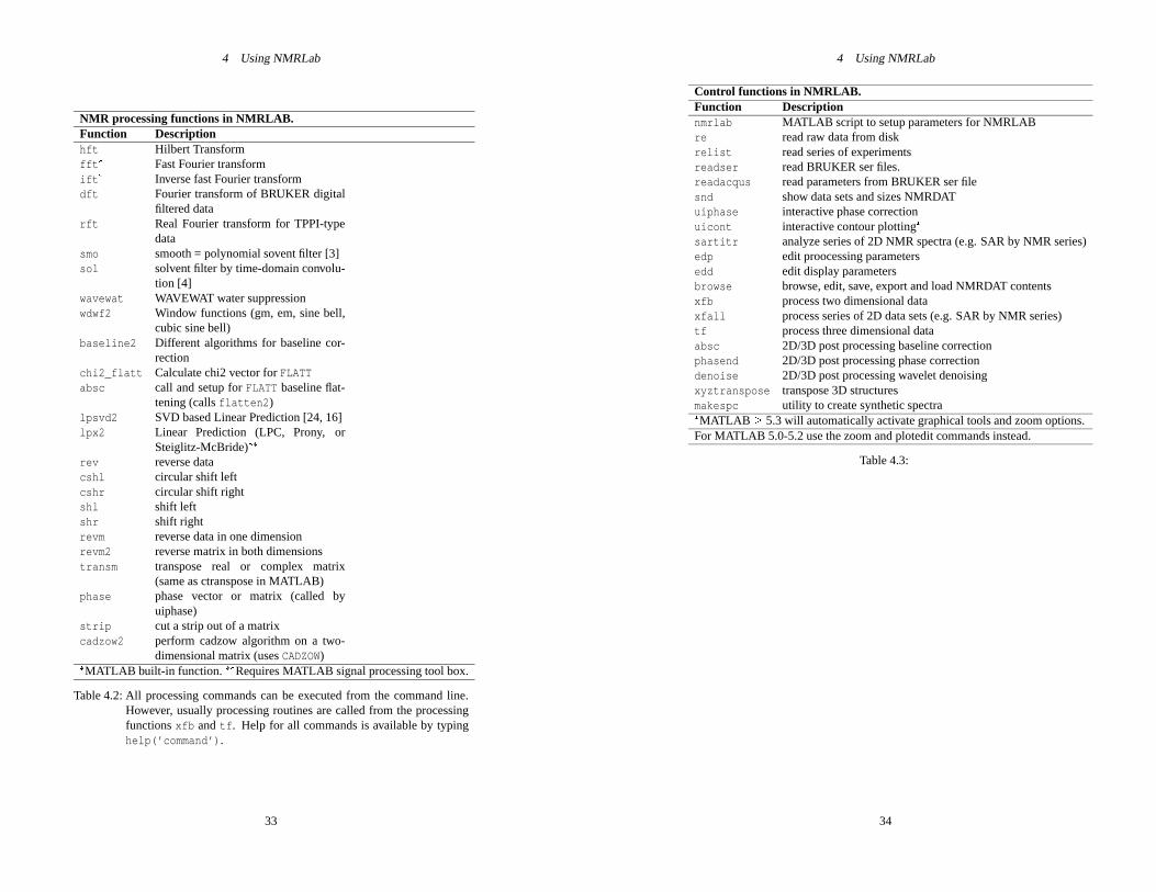
NMR processing functions in NMRLAB.Function Descriptionhft Hilbert Transformfft � Fast Fourier transformift � Inverse fast Fourier transformdft Fourier transform of BRUKER digital

filtered datarft Real Fourier transform for TPPI-type

datasmo smooth = polynomial sovent filter [3]sol solvent filter by time-domain convolu-

tion [4]wavewat WAVEWAT water suppressionwdwf2 Window functions (gm, em, sine bell,

cubic sine bell)baseline2 Different algorithms for baseline cor-

rectionchi2_flatt Calculate chi2 vector forFLATTabsc call and setup forFLATT baseline flat-

tening (callsflatten2 )lpsvd2 SVD based Linear Prediction [24, 16]lpx2 Linear Prediction (LPC, Prony, or

Steiglitz-McBride)��

rev reverse datacshl circular shift leftcshr circular shift rightshl shift leftshr shift rightrevm reverse data in one dimensionrevm2 reverse matrix in both dimensionstransm transpose real or complex matrix

(same as ctranspose in MATLAB)phase phase vector or matrix (called by

uiphase)strip cut a strip out of a matrixcadzow2 perform cadzow algorithm on a two-

dimensional matrix (usesCADZOW)

�MATLAB built-in function. ��Requires MATLAB signal processing tool box.

Table 4.2: All processing commands can be executed from the command line.However, usually processing routines are called from the processingfunctionsxfb and tf . Help for all commands is available by typinghelp(’command’) .

33

4 Using NMRLab

Control functions in NMRLAB.Function Descriptionnmrlab MATLAB script to setup parameters for NMRLABre read raw data from diskrelist read series of experimentsreadser read BRUKER ser files.readacqus read parameters from BRUKER ser filesnd show data sets and sizes NMRDATuiphase interactive phase correctionuicont interactive contour plotting�sartitr analyze series of 2D NMR spectra (e.g. SAR by NMR series)edp edit proocessing parametersedd edit display parametersbrowse browse, edit, save, export and load NMRDAT contentsxfb process two dimensional dataxfall process series of 2D data sets (e.g. SAR by NMR series)tf process three dimensional dataabsc 2D/3D post processing baseline correctionphasend 2D/3D post processing phase correctiondenoise 2D/3D post processing wavelet denoisingxyztranspose transpose 3D structuresmakespc utility to create synthetic spectra

�MATLAB � 5.3 will automatically activate graphical tools and zoom options.For MATLAB 5.0-5.2 use the zoom and plotedit commands instead.

Table 4.3:

34

4 Using NMRLab

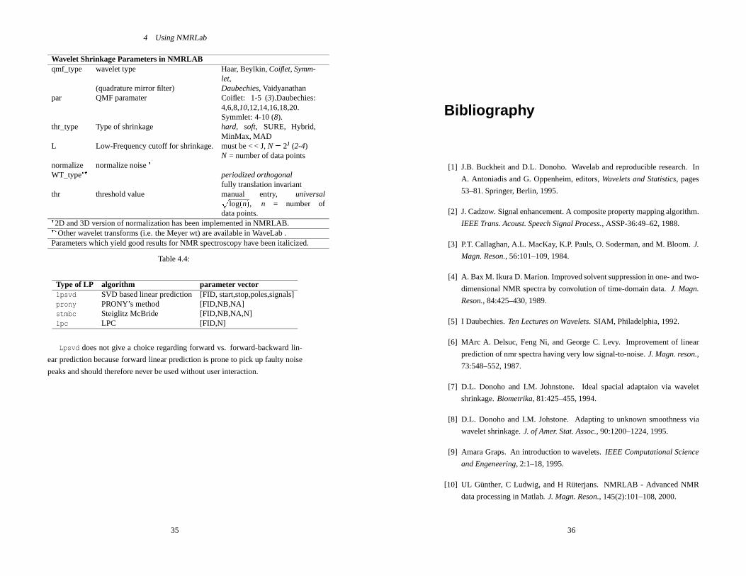
Wavelet Shrinkage Parameters in NMRLABqmf_type wavelet type Haar, Beylkin,Coiflet, Symm-

let,(quadrature mirror filter) Daubechies, Vaidyanathan

par QMF paramater Coiflet: 1-5 (3).Daubechies:4,6,8,10,12,14,16,18,20.Symmlet: 4-10 (8).

thr_type Type of shrinkage hard, soft, SURE, Hybrid,MinMax, MAD

L Low-Frequency cutoff for shrinkage. must be < < J,N = 2J (2-4)N = number of data points

normalize normalize noise�

WT_type�� periodized orthogonalfully translation invariant

thr threshold value manual entry, universalp

log(n), n = number ofdata points.

�2D and 3D version of normalization has been implemented in NMRLAB.

��Other wavelet transforms (i.e. the Meyer wt) are available in WaveLab .Parameters which yield good results for NMR spectroscopy have been italicized.

Table 4.4:

Type of LP algorithm parameter vectorlpsvd SVD based linear prediction [FID, start,stop,poles,signals]prony PRONY’s method [FID,NB,NA]stmbc Steiglitz McBride [FID,NB,NA,N]lpc LPC [FID,N]

Lpsvd does not give a choice regarding forward vs. forward-backward lin-

ear prediction because forward linear prediction is prone to pick up faulty noise

peaks and should therefore never be used without user interaction.

35

Bibliography

[1] J.B. Buckheit and D.L. Donoho. Wavelab and reproducible research. In

A. Antoniadis and G. Oppenheim, editors,Wavelets and Statistics, pages

53–81. Springer, Berlin, 1995.

[2] J. Cadzow. Signal enhancement. A composite property mapping algorithm.

IEEE Trans. Acoust. Speech Signal Process., ASSP-36:49–62, 1988.

[3] P.T. Callaghan, A.L. MacKay, K.P. Pauls, O. Soderman, and M. Bloom.J.

Magn. Reson., 56:101–109, 1984.

[4] A. Bax M. Ikura D. Marion. Improved solvent suppression in one- and two-

dimensional NMR spectra by convolution of time-domain data.J. Magn.

Reson., 84:425–430, 1989.

[5] I Daubechies.Ten Lectures on Wavelets. SIAM, Philadelphia, 1992.

[6] MArc A. Delsuc, Feng Ni, and George C. Levy. Improvement of linear

prediction of nmr spectra having very low signal-to-noise.J. Magn. reson.,

73:548–552, 1987.

[7] D.L. Donoho and I.M. Johnstone. Ideal spacial adaptaion via wavelet

shrinkage.Biometrika, 81:425–455, 1994.

[8] D.L. Donoho and I.M. Johstone. Adapting to unknown smoothness via

wavelet shrinkage.J. of Amer. Stat. Assoc., 90:1200–1224, 1995.

[9] Amara Graps. An introduction to wavelets.IEEE Computational Science

and Engeneering, 2:1–18, 1995.

[10] UL Günther, C Ludwig, and H Rüterjans. NMRLAB - Advanced NMR

data processing in Matlab.J. Magn. Reson., 145(2):101–108, 2000.

36

Bibliography

[11] UL Günther, C Ludwig, and H Rüterjans. Improved automatic structure

calculation usind wavelet denoised data.in preparation, 2001.

[12] UL Günther, C Ludwig, and H Rüterjans. WAVEWAT - Improved solvent

suppression in NMR spectra employing wavelet transforms.submitted to

J. Magn. Reson., 2001.

[13] W. Härdle, G. Kerkyacharian, D. Picard, and A. Tsybakov.Wavelets, Ap-

proximation, and Statistical Applications. Springer, 1998.

[14] Jeffrey C. Hoch and Alan S. Stern.NMR data processing. 1996.

[15] B Jawerth and W Sweldens. An overview of wavelet based multiresolution

analysis.SIAM Review, 36:377–412, 1994.

[16] R. Kumaresan and D.W. Tufts. Estimating the parametes of exponentially

damped sinosoids and pole-zero modelling in noise.IEEE Trans. Acoust.

Speech Signal Process., ASSP-30:833–840, 1982.

[17] S. Mallat.A wavelet tour of signal processing. Academic Press, 1998.

[18] Yves Nievergelt.Wavelets Made Easy. Birkhäuser, 1999.

[19] Todd R Odgen. Essential wavelets for statistical applications and data

analysis. Birkhäuser, 1997.

[20] WWF Pijnappel, A van den Boogaart, R de Beer, and D van Ormondt.

SVD-based quantification of magnetic resonance signals.J. Magn. Reson.,

97:122–134, 1992.

[21] Brani Vidakovic and Peter Müller. Wavelets for kids. Available at

http://www.isye.gatech.edu/ brani/wavelet.html, 1994.

[22] G. Zhu, W.Y. Choy, G. Song, and B.C. Sanctuary. Suppression of diagonal

peaks with singular value decomposition.J. Magn. Reson., 132:176–178,

1998.

[23] G Zhu, D Smith, and Y Hua. Post-acquisition solvent suppression by

singular-value decomposition.J. Magn. Reson., 124(1):286–9, 1997.

[24] Guang Zhu and Ad Bax. Improved linear prediction of damped nmr signals

using modified "forward-backward" linear prediction.J. Magn. Reson.,

100:202–207, 1992.

37