Journal of Biomolecular NMR, 2 (1992) 619-629 619 ESCOM

J-Bio NMR 094

Processing of multi dimensional NMR data with the new software PROSA

Peter Güntert, Volker Dötsch, Gerhard Wider and Kurt Wüthrich* Institut für Molekularbiologie und Biophysik, Eidgenössische Technische Hochschule-Hönggerberg,

CH-8093 Zurich, Switzerland

Received 1 September 1992 Accepted 28 October 1992

Keywords: Data processing; Fourier transformation; Linear prediction; Phase correction; Baseline correction

SUMMARY

The new program PROSA is an efficient implementation of the common data-processing steps for multi-dimensional NMR spectra. PROSA performs linear prediction, digital filtering, Fourier transformation, automatic phase correction, and baseline correction. High efficiency is achieved by avoiding disk storage of intermediate data and by the absence of any graphics display, which enables calculation in the batch mode and facilitates porting PROSA on a variety of different computer systems, including supercomputers. Furthermore, all time-consuming routines are completely vectorized. The elimination of a graphics display was made possible by the use of a new, reliable automatic phase-correction routine. CPU times for complete processing of a typical heteronuclear three-dimensional NMR data set of a protein vary between less than 1 min on a NEC SX3 supercomputer and 40 min on a Sun-4 computer system.

INTRODUCTION

Commonly available commercial software for the processing of NMR data makes use of graphics workstations (e.g., Hare Research Inc., 1990; TRIPOS Associates, Inc., 1992) or specialized computers connected to the spectrometers (e.g., Bruker Analytische Messtechnik GmbH, 1991). For NMR structure determinations of biological macromolecules (Wüthrich, 1986), which make extensive use of homonuclear and heteronuclear multi-dimensional NMR experiments for sequential resonance assignments and the collection of conformational restraints (Clore and Gronenborn, 1990; Fesik and Zuiderweg, 1990; Kay et al, 1990; Wüthrich, 1990), data processing

* To whom correspondence should be addressed. Abbreviations: 1D, one-dimensional; 2D, two-dimensional; 3D, three-dimensional; 4D, four-dimensional; NOESY, nuclear Overhauser enhancement spectroscopy; TOCSY, total correlation spectroscopy; TPPI, time-proportional phase incrementation; [u-BC]-, uniformly 13C-labeled

0925-2738/$ 5.00 © 1992 ESCOM Science Publishers B.V.

620

with these facilities requires large amounts of computation time. Because the aforementioned types of software rely on the use of a graphics display, they cannot readily be implemented on remote high-speed computers. In this paper, we present a new software package, PROSA, that can be readily implemented on different computers because it does not use computer graphics and, thanks to a novel, reliable automatic phase-correction routine, allows data processing in batch mode without interactive user intervention. Although PROSA is an efficient alternative for the processing of all types of high-resolution NMR data, it is particularly useful for large multi-dimensional data sets of macromolecules which require pre-processing with linear prediction and baseline correction.

METHODS

The program PROSA The new program package PROSA ('Processing algorithms') makes it possible to perform the

processing steps that lead from the time-domain data furnished by the NMR spectrometer to the multi-dimensional spectrum. Its functions include linear prediction, apodization, Fourier trans-formation, a new, automatic phase correction routine, baseline correction, and formatting of the output for easy use with spectrum analysis programs.

The design of the program is simple, both because it does not use computer graphics and because the complete multi-dimensional data matrix is kept in the memory throughout processing. Advantages of avoiding computer graphics are that the implementation of the program on a variety of different computers is straightforward, and that data processing can be done in the batch mode. The conventional interactive selection of phase-correction parameters (e.g., Bruker Analytische Messtechnik GmbH, 1991) is replaced by a reliable automatic phase-correction routine (see below). Keeping the complete data matrix in memory makes it possible, after suitable transpositions, to use identical input/output-free routines for processing in all dimensions of a multi-dimensional data set. The fully processed spectra can then be displayed on a conventional graphics station. In its present form the output of PROSA is compatible as input for the program package EASY (Eccles et al., 1991), which was recently extended for the analysis of 3- and 4D NMR spectra (C. Bartels and K. Wüthrich, unpublished results).

As PROSA completely avoids the need to store intermediate results on disk (i.e., at the outset the time-domain data are read into the computer memory and only the fully processed frequency-domain data are written back onto disk), the computer memory must be sufficiently large to hold the complete data set. The program is very efficient on vectorizing computers because of the complete vectorization of all time-consuming routines, which is facilitated by the fact that identical operations are applied independently to all 1D cross sections of a data set. As a consequence, the program can also readily be adapted for efficient parallel processing. PROSA is written in standard FORTRAN-77. So far, it can be used on a NEC SX3 supercomputer, and on Convex C2, Silicon Graphics and Sun-4 computers. PROSA is available for use in other laboratories upon request addressed to K. Wüthrich.

Linear prediction In PROSA, linear prediction (Stephenson, 1988; Olejniczak and Eaton, 1990; Zhu and Bax,

1990) is used to reduce effects caused by discrete Fourier transformation of truncated time-

621

domain signals, i.e., primarily line broadening and the appearance of side lobes. The linear prediction coefficients are determined by singular value decomposition (Kumaresan and Tufts, 1982; Press et al., 1986; Barkhuijsen et al., 1987). Since each individual coefficient represents one frequency component, it is necessary to have an approximate estimate of the number of frequencies included in the time-domain signal, and additional coefficients may be needed to account for noise. Singular value decomposition uses an overdetermined system of equations, and the maximal number of coefficients can be as high as one-half of the number of complex data points. To ensure that the predicted signal is stable, the roots of the characteristic polynomial of the linear prediction coefficients are calculated. Consistent with conventional use of linear prediction, PROSA takes all roots into account and guarantees a stable predicted signal by reflecting the roots z about the unit circle, z → z/|z|2, if necessary (Press et al., 1986). Although this procedure incorporates noise into the predicted data, the results usually do not differ significantly from those obtained when putative noise roots are eliminated, because the noise roots usually lead to rapidly decaying components of small intensity in the predicted data (Stephenson, 1988).

Since baseline distortions are primarily caused by errors in the measurement of the first few time-domain data points (Otting et al., 1986), the backward linear prediction implemented in PROSA can be used to restore this corrupted part of the signal, and is thus also a suitable method for baseline correction (Marion and Bax, 1989). When compared with baseline correction procedures that work in the frequency-domain (Pearson, 1977; Dietrich et al., 1991; Güntert and Wüthrich, 1992), an advantage of this method is that the baseline correction is performed at the start rather than at the end of data processing, which may improve the results of other processing steps that rely on a flat baseline.

Automatic phase correction Several algorithms for automatic phase correction with 1D NMR (Ernst, 1969; Neff et al., 1977;

Marshall and Roe, 1978; Gladden and Elliott, 1986; Brown et al., 1989; Nelson and Brown, 1989; Heuer, 1991) and 2D NMR (Cieslar et al., 1988; Hoffman et al., 1992) have been proposed. The new automatic phase-correction routine developed for PROSA determines the constant and linear phase-correction parameters, φο and φ1, by first searching the 1D cross sections of the power spectrum for strong, well separated peaks. Then, in the phase-sensitive spectrum, the sum S(φ0, φι) of the difference between the squared real and imaginary parts of the normalized integral over the peak region in the phase-corrected spectrum, Ip, is

is maximized. Ip denotes the integral over the region of the peak, p, in the spectrum before phase correction, and ωρ denotes the normalized position of peak ρ (Ο ≤ ωρ< 1). The summation runs over all peaks found to be acceptable for the purpose of phase correction (see below). The maximum of S(φ0, φ1) is obtained by selecting the linear phase correction, φ1, such that the function (2)

622

has its maximum absolute value at β = φ1 . The constant phase correction is set to φ0 = 1/2 arg s(φ 1 ), where arg s is the argument of the complex number s. Because s(β) usually has multiple local maxima, PROSA determines φ1 from a 1D grid search with a step size of ∆β (usually, ∆β = 1°). The method can be used for spectra containing both positive and negative peaks (but of course not for antiphase multiplets).

In practice, to determine peak positions in 1D cross sections of the power spectrum, the program first identifies all local maxima that are more than κ times above the noise level of the power spectrum (typically, κ = 10). For each maximum, the corresponding boundaries for peak integration are set at the first data points on either side that are lower than either 10% of the maximal peak intensity or twice the noise level. To decide which of the maxima correspond to suitable peaks for use in automatic phase correction, the following criteria are checked: (1) The width of the integration area must be smaller than a predetermined value, u; (2) To exclude overlapping peaks, the average intensity in the regions of width u/4 adjoining the integration area to the left and to the right must be either below 10% of the maximal peak intensity or below twice the noise level; (3) An upper limit, v, is imposed on the number of peaks that may have the same coordinates along one frequency axis (typically, ν = 20-50). If ν is exceeded, the program will only retain the ν highest peaks, so that the phasing cannot be dominated by one or several small spectral regions. The results of the automatic phase correction do not depend critically on the selection of the three parameters κ, u, and v. We found that the value of κ should be decreased for spectra with low signal-to-noise ratios, that the maximal peak width, u, should account for the increased line widths in power spectra, and that v can be reduced when a spectrum contains a large number of peaks. The number of 1D peaks included for the phase correction of a 3D spectrum is usually of the order of 1000, which renders the method robust against instabilities that might arise if only a small number of peaks were used, be it because of low signal-to-noise ratio, poor digital resolution, peak overlap, or occasional inclusion of artifactual peaks.

Baseline correction Baseline correction in the frequency domain is performed for each 1D cross section by first

identifying regions of 'pure baseline' (Güntert and Wüthrich, 1992) and then subtracting a function which is best-fitted to the pure baseline regions. The pure baseline regions are identified either with modified versions of the FLATT procedure (Güntert and Wüthrich, 1992) or with the 'derivative method' of Dietrich et al. (1991). For a data point k with intensity Sk both methods yield a parameter, pk, which becomes small if k is located in a pure baseline region, and large otherwise:

In Eq. 3, pk is determined by fitting a straight line, a + bl, to a stretch of 2n+1 data points centered about the data point, k. For the data points near the boundaries of the 1D cross section, where pk is not defined by Eq. 3, pk has the same value as the nearest data point inside the definition range. A minimal width for pure baseline regions (Güntert and Wüthrich, 1992) is ensured by smoothing pk:

623

pk = min(pk_n/3,..., pk + n/3) (FLATT); pk = max(min(pk,max(pk _ 1 ,pk + 1)), min(pk _ 1 ,pk + 1) (derivative method).

The definition of pk for the derivative method implies that any point at which both neighbors belong to pure baseline regions will also belong to it, and that there is no point in a pure baseline region for which both neighboring points do not belong to it (Dietrich et al., 1991). A cutoff, pc, is then defined such that pk ≤ pc for one-third of the data points and pk > pc for two-thirds of the data points, and all data points, k, that satisfy the relation pk ≤ τpc are considered as pure baseline, where τ is a user-defined parameter (typically, τ = 4). Any linear combination of functions that can be written as FORTRAN-77 arithmetic expressions may be used to represent the baseline distortions. Usually, we use the constant and the trigonometric functions corresponding to the first m time-domain data points (see Eq. 4 in Güntert and Wüthrich, 1992). The linear least-squares fit to the pure baseline regions is solved by standard techniques, using singular value decomposition (Press et al., 1986).

RESULTS AND DISCUSSION

An illustration of the practical use of the program PROS A is afforded by the processing of a 4D [13C,13C]-correlated [1H,1H]-NOESY (Clore et al., 1991; Zuiderweg et al., 1991) data set of a complex formed by the uniformly 13C-labeled protein cyclophilin and the unlabeled immunosuppres-sive drug cyclosporin A, which was recorded on a Bruker AMX 500 spectrometer (C. Spitzfaden, G. Wider and K. Wüthrich, unpublished results). Table 1 lists the sequence of PROSA commands used for data processing. In its present version, the program reads or writes serial input files in the integer format written by Bruker X32 computers, serial integer and real data, and submatrix files in the format used by the program EASY (Eccles et al., 1991; C. Bartels and K. Wüthrich, unpublished results), using 8 or 16 bits per data point. The extension to other input file formats is straightforward because the program only needs the data itself, i.e., it does not require additional information from headers or separate parameter files. Most PROSA commands are applied to only one dimension of the multi-dimensional data set, i.e. the active dimension selected by the operator. Internally, the program handles the data as a 2D matrix, where the data points of the active dimension are stored sequentially in the computer memory. The command dimension selects the active dimension by transposing the multi-dimensional data matrix. For apodization prior to Fourier transformation, any function that can be written as a FORTRAN-77 arithmetic expression may be used, including the commonly used window functions (De Marco and Wüthrich, 1976; Ernst et al., 1987). To facilitate the use of the program, the most common apodization functions are implemented as macros. These are files that contain PROSA commands such as multiply, which multiplies part or all of the data points with a constant or variable factor:

multiply fk k1 k2 k3 (5)

The command (5) multiplies the k-th data point by a factor fk, where k runs from data point k1 to data point k2 in steps of k3 (if k 1 , k2, and k3 are omitted, all data points are multiplied; if only k1 is given, the data point k1 is multiplied; if k3 is omitted, the program assumes k3 = 1). For example, a cosine window function (the macro call cos in Table 1) is represented by multiply

aCyclophilin was complexed with unlabeled cyclosporin A. The resulting spectra are illustrated in Figs. 1 and 2. ω1 and ω2 = 13C, ω3 and ω4 = Ή.

b The dimension to which a command is applied. For transpositions, the change of the active dimension is indicated. c In its present version, the program accepts serial input files from Bruker X32 computers, serial integer and real data, and submatrix files in the format used by the program EASY. d The States-TPPI method for quadrature detection in the

indirectly detected dimensions is a combination of the States method and the TPPI method. The multiplication is necessary for obtaining a conventional spectrum by complex Fourier transformation (Marion et al., 1989).

624

625

cos($pi/(2*$n)*(k-1)), where $pi = π, $η denotes the number of data points, and k runs over all data points. Other uses of the multiply command include scaling of the complete spectrum (multiply 0.01 in Table 1), the correct weighting of the first time-domain data point prior to Fou-

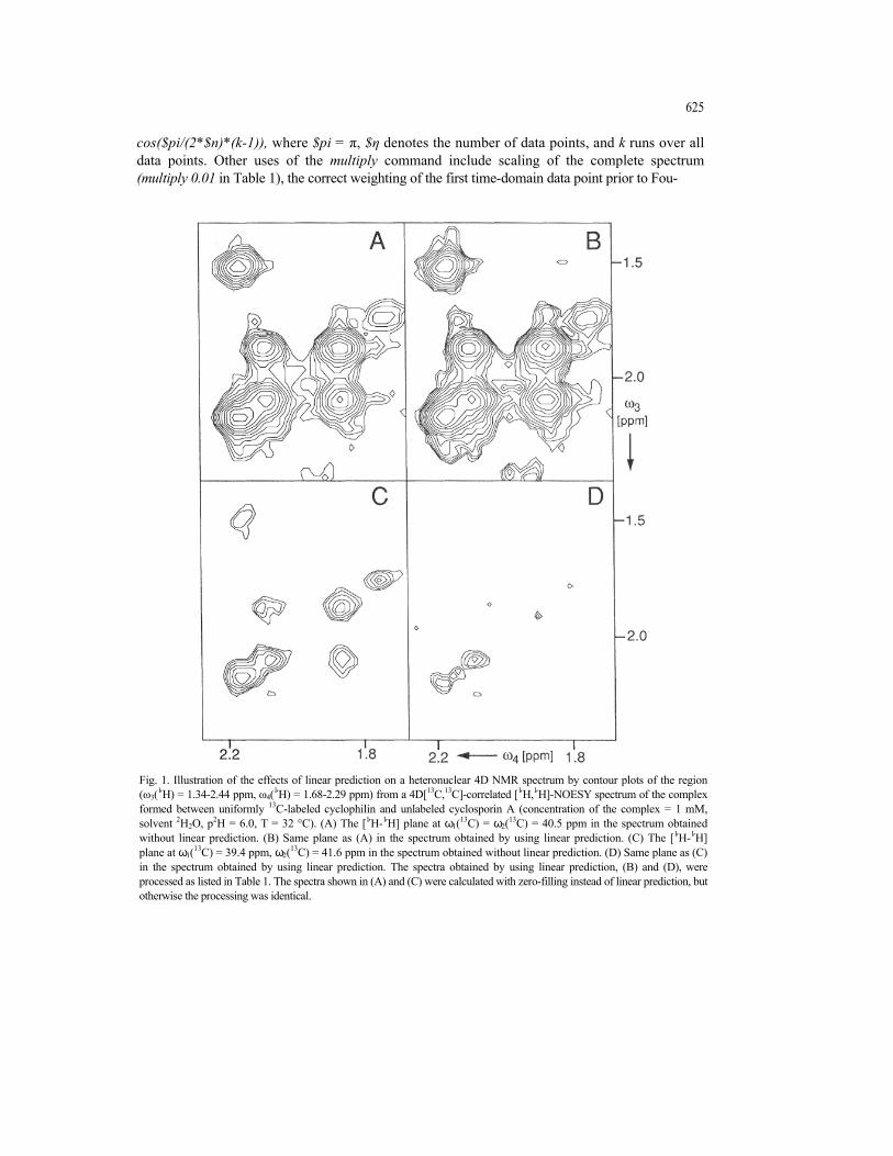
Fig. 1. Illustration of the effects of linear prediction on a heteronuclear 4D NMR spectrum by contour plots of the region (ω3(1Ή) = 1.34-2.44 ppm, ω4(1Ή) = 1.68-2.29 ppm) from a 4D[13C,13C]-correlated [1Ή,1Ή]-ΝΟΕSΥ spectrum of the complex formed between uniformly 13C-labeled cyclophilin and unlabeled cyclosporin A (concentration of the complex = 1 mM, solvent 2H2O, p2H = 6.0, Τ = 32 °C). (A) The [1Ή-1Ή] plane at ω1(13C) = ω2(13C) = 40.5 ppm in the spectrum obtained without linear prediction. (B) Same plane as (A) in the spectrum obtained by using linear prediction. (C) The [1Ή-1Ή] plane at ω1(13C) = 39.4 ppm, ω2(13C) = 41.6 ppm in the spectrum obtained without linear prediction. (D) Same plane as (C) in the spectrum obtained by using linear prediction. The spectra obtained by using linear prediction, (B) and (D), were processed as listed in Table 1. The spectra shown in (A) and (C) were calculated with zero-filling instead of linear prediction, but otherwise the processing was identical.

626

rier transformation to avoid ridges in the spectrum (Otting et al., 1986) (multiply 0.5 l in Table 1), the change of sign of every second data point when using the States-TPPI method for quadrature detection (Marion et al., 1989) (multiply - 1 2 n 2 in Table 1), and phase correction if the phase-correction parameters are already known, for example, by appropriate selection of the initial delay in the pulse sequence (Bax et al., 1991). The program PROSA provides real and complex fast Fourier transformation and inverse Fourier transformation (Press et al., 1986). Zero-filling,

Fig. 2. Cross sections from the 4D [13C,13C]-correlated [1Ή,1Ή]-ΝΟΕSΥ spectrum of the [u-13C]-cyclophilin-cyclosporin A complex of Table 1, which illustrate the effects of the automatic phase correction in all dimensions. Negative peaks represent folded lines. In all examples, (A)-(F), the full spectral width is shown, and the dotted line indicates zero intensity. (A) Cross section along ω4(1Ή), with ω1(13C) = 37.1 ppm, ω2(13C) = 36.1 ppm, and ω3(1Ή) = 4.37 ppm. (B) Cross section along ω3(1Ή), with ω1(13C) - 34.9 ppm, ω2(13C) = 41.6 ppm, and ω4(1H) = 1.06 ppm. (C) Cross section along ω2(13C), with ω1(13C) = 40.5 ppm, ω3(1Ή) = 1.01 ppm, and ω4(1Ή) = 4.49 ppm. (D) Cross section along ω2(13C), with ω1(13C) = 31.7 ppm, ω3(Ή) = 1.86 ppm, and ω4(1Ή) = 2.33 ppm. (E) Cross section along ω1(13C), with ω2(13C) = 39.6 ppm, ω3(1Ή) = 1.63 ppm, and ω4(1Ή) = 4.01 ppm. (F) Cross section along ω1(13C), with ω2(13C) = 32.1 ppm, ω3(1Ή) = 2.56 ppm, and ω4(1Ή) = 1.93 ppm.

627

strip transform, and phase correction with known phase parameters can be included in the Fourier transform command, which may avoid the temporary need of extra memory.

Because only 2D planes from a multi-dimensional spectrum can readily be displayed with a computer graphics system, peaks with broad or rippled lineshapes along the dimensions perpen-dicular to the viewing plane may render the manual interpretation of 3D and in particular 4D spectra tedious. Therefore, linear prediction of the time-domain signal prior to Fourier transfor-mation, which yields narrower and ripple-free lines, can greatly facilitate the interpretation of the spectra. As an example, Fig. 1 shows regions from the 4D [13C,13C]-correlated NOESY spectrum of a [u-13C]-cyclophilin-cyclosporin A complex (Table 1), illustrating the improved quality of the spectrum obtained by linear prediction in both 13C dimensions when compared to simple zero-filling. In Figs. 1A and 1B, a 1Ή-1Ή region from the 6th out of a total of 16 planes along ω1 and ω2 is displayed, which contains several peaks on resonance with respect to the 13C frequencies. It is seen that, in this case, there is little difference between the spectra obtained with or without use of linear prediction. In contrast, Figs. 1C and 1D, which display the same [1Ή-1Ή] region from the 7th plane along ω1 and the 5th plane along ω2, i.e., off resonance relative to the 13C frequencies, show a significant reduction in the number of artifactual peaks after linear prediction. Most of the 'signals' in Fig. 1C are effectively tails of peaks that have their maximal intensity in the 1H-1H plane shown in Fig. 1 A.

TABLE 2 CPU TIMES USED FOR THE PROCESSING OF MULTI-DIMENSIONAL NMR DATA SETS WITH THE PRO-GRAM PROSA Input data size Computer CPU time [s]a

[complex data points]Output data size Total Linear Fourier Phase Baseline [real data points] prediction transform correction correction 256 x 110 x 8 x 6b NEC SX3 574 285 18 92 144 (512 x 256 x 16 x 16) 512 x 80 x 8C NEC SX3 39 11 1.2 7 16

(512 x 256 x 32) Convex C2 600 258 23 69 179 Sun-4/690 2093 1052 114 87 644 2048 x 391d NEC SX3 4.5 _ 0.7 0.8 2.0 (2048 x 512) Convex C2 80 - 16 10 29 Iris 4D/35 300 _ 77 19 143 Sun-4/690 343 - 86 22 156

a The total time used and the times used by the four most time-consuming routines are listed (see text). b 4D [13C,13C]-correlated [1H,1H]-ΝΟΕSΥ spectrum of a [u-13C]-cyclophilin-cyclosporin A complex (C. Spitzfaden,

G. Wider and K. Wüthrich, unpublished results). The data processing steps are listed in Table 1. c 3D HCCH-TOCSY (Bax et al., 1990) of a [u-13C]-cyclophilin-cyclosporin A complex (C. Spitzfaden, G. Wider and

K. Wüthrich, unpublished results). Linear prediction with three coefficients was used to predict eight data points in ω1. Fourier transformation, automatic phase correction, and baseline correction were used in all three dimensions. d 2D[1H,1H]-

NOESY spectrum of the 434 repressor(l-63) in H2O (O. Schott, V. Dötsch and K. Wüthrich, unpublished results). Fourier transformation, automatic phase correction, and baseline correction were used in both dimensions.

628

The automatic phase-correction routine of PROSA was used in all four dimensions of the 4D spectrum of Table 1. One dimension cross sections through the spectrum (Fig. 2) demonstrate that the automatic phase-correction routine produced pure absorptive line shapes in all dimen-sions. The routine worked reliably regardless of the number of data points contained in the 1D cross sections.

Table 2 lists the CPU times required for complete processing of three different NMR data sets using PROSA on different computers. The 4D [13C,13C]-correlated [1H,1H]-NOESY spectrum of a [u-13C]-cyclophilin-cyclosporin A complex (Table 1) was selected as an example of a large data set, a 3D HCCH-TOCSY spectrum (Bax et al., 1990) of the same complex (C. Spitzfaden, G. Wider and K. Wüthrich, unpublished results) as a representative 3D spectrum of a protein, and a homonuclear 2D NOESY spectrum of the 434-repressor (1-63) (O. Schott, V. Dötsch and K. Wüthrich, unpublished results) as a typical spectrum used to obtain conformational constraints for the structure determination of a small protein. Fourier transformation, automatic phase correction, and baseline correction were applied to all data sets; linear prediction was used in all 13C dimensions of the 4D and 3D data sets. On the NEC SX3 supercomputer, the CPU times for the processing of the three spectra were less than 10 min, less than 40 s, and less than 5 s, respectively. The 3D and 2D spectra were also processed on a Convex C2, a Silicon Graphics and a Sun computer, which used between 15 and 76 times more CPU time than the NEC SX3. Table 2 also gives separate CPU times for linear prediction, Fourier transformation, automatic phase correction, and baseline correction. The most time-consuming steps on all computers were linear prediction and baseline correction, which took 28-50% and 25-45% of the total CPU time, respectively, whereas the Fourier transformations took less than 6% of the CPU time for the 3D and 4D data sets, and 16-26% for the 2D data set. The automatic phase-correction routine needed between 4 and 18% of the total CPU time. The data of Table 2 can be evaluated in the context of earlier reports that on Sun-4 computer systems, CPU times in the range of 8-32 h are needed for linear prediction with singular value decomposition of 'typical' heteronuclear 3D spectra of proteins (Zhu and Bax, 1990).

ACKNOWLEDGEMENTS

We thank Claus Spitzfaden and Oliver Schott for the use of unpublished spectra of cyclophilin and the 434 repressor(l-63), respectively. We acknowledge financial support from the Schweizer-ischer Nationalfonds (project 31.32033.91) and the Stipendienfonds der deutschen chemischen In-dustrie (fellowship to V.D.). The use of the NEC SX3 supercomputer of the Centro Svizzero di Calcolo Scientifico is gratefully acknowledged.

REFERENCES

Barkhuijsen, H., De Beer, R. and van Ormondt, D. (1987) /. Magn. Reson., 73, 553-557. Bax, A., Clore, G.M. and Gronenborn, A.M. (1990) /. Magn. Reson., 88, 425-431. Bax, A., Ikura, M., Kay, L.E. and Zhu, G. (1991) /. Magn. Reson., 91, 174-178. Brown, D.E., Campbell, T.W. and Moore, R.N. (1989) /. Magn. Reson., 85, 15-23. Bruker Analytische Messtechnik GmbH (1991) UXNMR. Messen und Verarbeiten von NMR Daten, Rheinstetten,

Germany. Cieslar, C., Clore, G.M. and Gronenborn, A.M. (1988) /. Magn. Reson., 79, 154-157.

629

Clore, G.M. and Gronenborn, A.M. (1991) Prog. NMR Spectrosc., 23, 43-92. Clore, G.M., Kay, L.E., Bax, A. and Gronenborn, A.M. (1991) Biochemistry, 30, 12-18. DeMarco, A. and Wüthrich, K. (1976) /. Magn. Reson., 24, 201-204. Dietrich, W., Rudel, C.H. and Neumann, M. (1991) /. Magn. Reson., 91, 1-11. Eccles, C., Gümtert, P., Billeter, M. and Wüthrich, K. (1991) /. Biomol NMR, 1, 111-130. Ernst, R.R. (1969) /. Magn. Reson., 1, 7-26. Ernst, R.R., Bodenhausen, G. and Wokaun, A. (1987) Principles of Nuclear Magnetic Resonance in One and Two Dimensions,

Clarendon Press, Oxford. Fesik, S.W. and Zuiderweg, E.R.P. (1990) Quart. Rev. Biophys., 23, 97-131. Gladden, L.F. and Elliott, S.R. (1986) /. Magn. Reson., 68 383-388. Güntert, P. and Wüthrich, K. (1992) /. Magn. Reson., 96, 403-407. Hare Research Inc. (1991) FELIX User Documentation. Version 2.0, Woodinville, WA, U.S.A. Heuer, A. (1991) /. Magn. Reson., 91, 241-253. Hoffman, R.E., Delaglio, F. and Levy, G.C. (1992) /. Magn. Reson., 98, 231-237. Kay, L.E., Ikura, M., Tschudin, R. and Bax, A. (1990) /. Magn. Reson., 89, 496-514. Kumaresan, R. and Tufts, D.W. (1982) IEEE Trans. Acoust. Speech Signal Process., 30, 833-840. Marion, D. and Bax, A. (1989) /. Magn. Reson., 83, 205-211. Marion, D., Ikura, M., Tschudin, R. and Bax, A. (1989) /. Magn. Reson., 85, 393-399. Marshall, A.G. and Roe, D.C. (1978) Anal. Chem., 50, 756-763. Neff, B.L., Ackerman, J.L. and Waugh, J.S. (1977) /. Magn. Reson., 25, 335-340. Nelson, S.J. and Brown, T.R. (1989) /. Magn. Reson., 84, 95-109. Olejniczak, E.T. and Eaton, H.L. (1990) /. Magn. Reson., 87, 628-632. Otting, G., Widmer, H., Wagner, G. and Wüthrich, K. (1986) /. Magn. Reson., 66, 187-193. Pearson, G.A. (1977) /. Magn. Reson., 27, 265-272. Press, W.H., Flannery, B.P., Teukolsky, S.A. and Vetterling, W.T. (1986) Numerical Recipes: The Art of Scientific Com-

puting, Cambridge University, Press, Cambridge. Stephenson, D.S. (1988) Prog. NMR Spectrosc., 20, 515-626. TRIPOS Associates, Inc. (1992) SYBYL/NMR TRIAD, St. Louis, MO, U.S.A. Wüthrich, K. (1986) NMR of Proteins and Nucleic Acids, Wiley, New York. Wüthrich, K. (1990) /. Biol Chem., 265, 22059-22062. Zhu, G. and Bax, A. (1990) /. Magn. Reson., 90, 405-410. Zuiderweg, E.R.P., Petros, A.M., Fesik, S.W. and Olejniczak, E.T. (1991) /. Am. Chem. Soc., 113, 370-372.