context-aware fault localization via control flow analysis

Context-Aware Fault Localization via Control Flow Analysis

Lei Zhao, Lina Wang, Xiaodan Yin School of Computer, Wuhan University

Key Laboratory of Aerospace Information Security and Trust Computing, Ministry of Education Wuhan 430072, P.R.China

Email: [email protected], [email protected], [email protected]

Abstract—Coverage-based fault localization techniques are effective to support program debugging. However, these techniques assess the suspiciousness of program entities individually. Such calculation oversimplifies executions and cannot reflect execution contexts. In this paper, we use control flow paths to analyze the execution context, quantify edge profiles to assess how each block contributes to failures and propose the context-aware fault localization approach FP. We use the edge profile to represent the passed and failed executions, calculate the coverage statistics and edge suspiciousness scores, and then by contrasting edge suspiciousness scores of blocks covered by a failed execution, we propose fault proneness to evaluate how each block contributes to the failure. At last, we take the sum of fault proneness as the suspiciousness to assess the probability of containing faults. We construct controlled experiments to compare our technique with a representative technique. The findings are as follows. 1) the FP technique performs well in locating faults if the infected state propagation is complex, 2) but when the fault is easy to locate, the FP technique may be overly complicated, 3) the integration of the two techniques are more effective than any of them. Index Terms—program debugging, fault localization, fault proneness, control flow analysis

I. INTRODUCTION

Program debugging is a tedious, challenging and error-prone process in software development. It is desirable to automate the debugging as much as possible. Fault localization is the vital step of debugging [1]. It aims to filter statements unrelated to bugs and locate only the remaining statements to be further examined.

Coverage based fault localization (CBFL) techniques have been proposed to support program debugging [2]. CBFL techniques usually contrast the program spectra information (such as coverage statistics) between passed and failed executions to compute the suspiciousness of individual program entities (such as statements, blocks and predicates), and then they construct a list of program entities in descending order of their fault suspiciousness. Programmers may follow the suggested list to locate faults. Empirical studies have shown that CBFL techniques can be effective in guiding programmers to examine code and locate faults.

However, the coverage statistics of program entities are calculated individually. For all the entities that are

executed in a failed execution, the number of failed executions will be equally added by 1. Several studies have proposed that such calculation ignores the dependency relationships between the predecessor and successor entities, which may result that the located entity is not the root cause of failure. For example, CBFL techniques are always able to locate the entities at which the program fails, but these entities do not contain faults [5].

In addition, with the impact of random test cases, the individual coverage statistics cannot reflect the similarity of executions [7]. We take an example as follows for detailed illustration. The number of failed executions that cover the entity b is noted as failed (b) =n. The n failed executions may follow n different control flow paths that cover b. Also, the n failed executions can just follow the same path that covers b. In the two cases, the number of failed executions that executed b is n. However, if the n failed executions follow the same path, the coverage statistics of all the program entities covered by the path are n. So the programmer still cannot locate the entity containing the fault. On the contrary, if the n failed executions follow n different paths that cover n, we can infer that b is more likely containing faults because n different executions are failed. That is to say, the difference between the case that n failed executions follow the same path and the case that n failed executions follow n different path is distinct. Therefore, we claim that to enable the execution context analysis during the coverage statistics is significant to improve CBFL techniques.

The control flow path is an appropriate way to solve the above problem. If b contains a fault, all execution paths that cover b may trigger the fault and perform failure [11]. On the contrary, if b is fault free, even if b is executed in a failed execution, the possibility that all the executions are failed is rather low. To sum up, the coverage statistics to paths can indicate how infected states propagate to failure and further indicate the fault proneness of blocks. The passed and failed executions covering a block are not identical for every entity, so the fault proneness of entities covered by a failed execution is different from each other. Capturing this characteristic, we propose a context-aware fault localization approach via path analysis.

Our approach uses the program control flow graph to

JOURNAL OF SOFTWARE, VOL. 6, NO. 10, OCTOBER 2011 1977

© 2011 ACADEMY PUBLISHERdoi:10.4304/jsw.6.10.1977-1984

organize the coverage and calculate edge suspiciousness. Given a failed execution, we use the fault proneness to assess how each block covered by this execution contributes to the failure by contrasting the coverage statistics of different edges covering the block. The sum of all fault proneness for every failed execution is defined as suspiciousness, and finally we synthesize a ranked list to facilitate fault localization. At last, we construct controlled experiments to validate the effectiveness of our approach. The main contributions of this paper include three aspects: 1) by contrasting the coverage statistics of different edges covering the block, we propose an approach to assess the fault proneness of blocks covered by the same execution. 2) The experiment results show that our approach is promising when dealing with faults which are hard to localize with the Tarantula technique. 3) Besides, the experiment results also indicate that the FP works better if integrated with CBFL techniques such as Tarantula.

The paper is organized as follows: Section 2 gives related work and a motivation example. Section 3 presents our analysis model and the FP technique, followed by some experimental evaluations and discussion in Section 4. Section 5 concludes this paper and presents our future work.

II. RELATED WORK AND MOTIVATION

A. Coverage based Fault Localization Agrawal et al. [1] are the first to propose the coverage

based fault localization technique, which is called χSlice. In this technique, the set of statements executed only in the failed test run, is reported as the likely faulty statements. This idea is further developed by Renieris and Reiss [18]. They propose the Nearest Neighborhood (NN) technique, which selects the nearest passed execution. Jones and colleagues [13] propose a different CBFL technique called Tarantula. Tarantula uses the coverage statistics and ratio of failed executions to predicate the suspiciousness of program failures. Researchers propose new CBFL techniques, such as Ochiai and Jaccard [3], which are similar to Tarantula except that they use different formulas to compute the suspiciousness. Existed experiment results show that when multiple test runs are available, the performance of CBFL is better than delta debugging and program slicing based techniques [2].

Tarantula and other similar fault localization techniques such as SBI are statements level. Statistical debugging instruments predicates into program code and locates faults by comparing the evaluation results of predicates in failed test runs with those in all test runs [14][20][21]. Predicates can be regarded as another manner of coverage refinement by exploiting the program state information. Santelices et al. investigate the effectiveness of using different program entities to locate faults. They show that the integrated results of using different program entities may be better than the use of any single kind of program entity [4].

The path and edge profiles have also been used in previous studies, which are similar to our technique in this paper. Jiang and Su propose a technique which uses

clustering to obtain fault predictors with the biggest fault proneness, and then generate the execution paths that traverse these predicates to reflect how the failure occurs [8]. George and his colleagues propose the program dependence graph (PPDG) that facilitates probabilistic analysis and reasoning about uncertain program behavior, particularly behavior that associated with faults. The PPDG could be applied to fault diagnosis [22]. Chilimbi et al. [12] believe that there are more meaningful information in execution report based on path than execution report based on block, and propose the HOLMES framework. The statements are examined according to the suspiciousness of path which covers them. Zhang et al. [5] propose the idea of propagation of infected states, which is very novel. Getting inspiration from it, we design the suspiciousness calculation of paths.

B. Motivating Example In this section, we will take an example to illustrate our motivation.

The statements shown in Figure 1 are a real program segment of grep, which is a Linux program. Among the statements, the operation '||' in the if condition statement should be '&&'. The control flow graph is shown in Figure 1. When examining the coverage information, we find that the if condition statement is always executed in either failed execution or passed executions. According to the coverage information, the suspiciousness score of b2 cannot be assured to be larger than other blocks when the coverage statistics based techniques are employed such as Tarantula [13] and SBI [3].

We note that the failed executions covering b3 is failed (b3), the passed executions covering b3 is passed (b3). According to SBI, the suspiciousness score of b3 is failed (b3)/ (failed (b3) + passed (b3)). Similar, the suspiciousness score of b2 is failed (b2)/ (failed (b2) + passed (b2)). Because failed (b2) = failed (b3) + failed (b4), and passed (b2) = passed (b3) + passed (b4), the suspiciousness of b2 will be no larger than the larger one of b3 and b4.

In fact, the failed executions of b3 and b4 are caused by the faulty condition which is generated in b2, so the suspiciousness of b2 should be larger in ideal fault localization method.

Examining the executions of the scheduled program, there are two failed execution paths, which are b1→b2→b4 and b1→b2→b3. Suppose that the fault exists in b2, the infected program state may be generated after b2 has been executed, and the infected state can propagate to b3 and b4 along with the path b2→b3 and b2→b4. It means

Figure 1 The motivation example

1978 JOURNAL OF SOFTWARE, VOL. 6, NO. 10, OCTOBER 2011

© 2011 ACADEMY PUBLISHER

that there should be several failed executions along with b1→ b4, and this is in accordance with the actual executions. In contrast, if we suppose that b3 contains a fault, there should not be failed executions along with b2→b4. These suppositions are not supported by the actual executions as shown in Figure 1.

According to the above analysis, the coverage statistics to different edges can indicate how infected states propagate to failure and further indicate the probability of containing faults. The qualified value is noted as the fault proneness as defined in Section 3.

III. METHODOLOGY

A. Preliminaries

Definition 1 A basic block, also known as a block, is a sequence of consecutive statements or expressions containing no transfer of control except at the end.

Given that the programs do not fail with crash fault, if one element (statement) of a block is executed, all the other elements are also executed. This definition has also been used in related researches [3][5].

Definition 2 EG={B,E,Path} is used to denote the execution graphs in this paper, where B={ b1, b2, …, bm} is the set of basic blocks of the program, Path={ path1, path2, …, pathn} is the set of execution paths, and E={e1, e2, …, ek} is the path edges that start from one block to another.

In the rest of this paper, the notation e (bi, bj) is usually used to represent the edge that goes from block bi to block bj. The notation e (*, bj) is used to represent all the edges that go to bj. The notation e (bi,*) is used to represent all the edges that start from bi. Besides, the edge e (bi, bj) is covered means e (bi, bj) has been executed in the execution.

Definition 3 The two blocks linked by an edge are named as successive blocks. The block from which the edge starts is named as the predecessor block while the other is named as the successor block.

Definition 4 The fault proneness expresses the quantified value of how blocks contribute to a certain failed executions. The larger the fault proneness of a block is, the larger possibility of a block containing the fault causing failure.

All the blocks covered by failed executions are likely to contain faults, but in many situations, only a certain block contains a fault. By employing the concept of fault proneness, we want to quantify how each block contributes to the failed execution, and in this way, we can distinguish the block that most likely contains fault from other blocks covered by the failed execution.

Definition 5 The fault suspiciousness is defined to represent the probability of a block containing faults.

The fault proneness just indicates how blocks contribute to a failed execution. For different failed executions, the fault proneness of a block may be

different. As a result, the fault suspiciousness value must be normalized to accumulate different fault proneness.

B. Analysis Model In this section we use the failed execution edge shown

in Figure 2 to illustrate the computing process of fault proneness. We note ( , )e s d as a failed execution edge as shown in Figure 2. There must be a fault in either s or d . The fault localization is used to determine which node has more possibilities to lead to the failed execution and which node has higher fault proneness. If the fault is located at s instead of d , then other execution edges which cover s are likely to trigger the fault in s and lead to failed executions. At the same time, the executions which cover d instead of s may be passed executions. On the contrary, if the fault is located at d instead of s , then the executions which cover s are likely to be passed executions while executions covering d may be failed executions. In brief, if most of executions which cover s are passed executions while executions covering d are failed executions, the fault is more likely to be located at d . Also, if most of executions which cover s are failed executions while executions covering d are passed executions, the fault is more likely to be located at s . Therefore, the fault proneness of d and s can be measured through analyzing the coverage statistics of execution edges which cover s and those of execution edges which cover d . As a result, the comparison of coverage statistics between execution edges covering s and d can be taken as the quantification of fault proneness.

C. Edge Suspiciousness Calculation Based on the conclusion in section 3.1, how to

calculate the distribution probability of failed execution paths becomes an urgent problem. In this section, we first show the computing method of how to obtain the suspiciousness in an execution flow diagram. Existing researches indicate that it is not appropriate to use the coverage frequency as the fault coverage rate in an edge. In this paper, we choose the suspiciousness definition formula mentioned in [5] to solve this problem.

( )( ) ( )

ii

i i

failed ee

failed e passed eθ( ) =

+ (1)

As shown above, ( )ifailed e represents the number of failed executions that cover ie , and ( )ipassed e represents

Figure 2 An illustration example



the number of passed executions that cover ie .

D. Quantification of fault Proneness Let us reexamine the executions which are shown in

Figure 2. The notation ( ( , ))inprob e s d is used to represent the proportion of ( ( , ))e s dθ to ( (*, )e dθ , which is the sum of edge suspiciousness values of all edges which go to d . The notation ( ( , ))outprob e s d is used to represent the proportion of ( ( , ))e s dθ to ( ( ,*))e sθ , which is the sum of edge suspiciousness values of all edges which start from s . In this example, ( ( ,*))e sθ includes 1( ( , ))e s dθ , and ( ( , ))e s dθ . ( (*, ))e dθ includes 1( ( , ))e s dθ , 2( ( , ))e s dθ and ( ( , ))e s dθ .

If all the executions along 1( , )e s d and 2( , )e s d are passed executions while the executions along

1( , )e s d and 2( , )e s d are failed executions, then d has the higher fault proneness. According to Equation (1), the value of both 1( ( , ))e s dθ and 2( ( , ))e s dθ are equal to 0, while the value of 1( ( , ))e s dθ and 2( ( , ))e s dθ are larger than 0. In such case, the value of ( ( , ))inprob e s d is less than ( ( , ))outprob e s d . By contrast, if all the executions along 1( ( , ))e s dθ and 2( ( , ))e s dθ are failed executions while the executions along 1( ( , ))e s dθ and 2( ( , ))e s dθ are passed executions, then s has higher fault proneness. In this case, the value of ( ( , ))inprob e s d is larger than ( ( , ))outprob e s d . In conclusion, the value of

( ( , ))inprob e s d and ( ( , ))outprob e s d can be used to indicate the fault proneness of s and d , respectively. The next, we will use ( ( , ))inprob e s d and ( ( , ))outprob e s d to qualify the values of fault proneness of s and d . The equation of ( ( , ))inprob e s d is given as below.

(*, )

(*, )

( ( , ))( ( , ))

[ ( (*, ))]e d

ine d

e s dprob e s d

e d

θ

θ∀

∀

∗=

∑∑

(2)

, where ( ( , ))e s dθ represents the edge suspiciousness of ( , )e s d ,

(*, )[ ( (*, ))]

e de dθ

∀∑ represents the sum of

suspiciousness of all the edges that go to d , and

(*, )e d∀∑ represents the number of edges that go

to d . The reason for setting (*, )e d∀∑ in Equation (2) is

to deal with the case that ( ( , )) 0e s dθ = . Take the example shown in Figure 2. If 1( ( , )) 0e s dθ = and 2( ( , )) 0e s dθ = , the value of Equation (2) equals 3. If

(*, )e d∀∑ is not set

in Equation (2), the value equals 1, which cannot be distinguished from the case that there are only one edge that goes to d . Actually, that 1( ( , )) 0e s dθ = and 2( ( , )) 0e s dθ = indicates that s may have higher fault proneness. It satisfies the equation value of Equation (2).

The equation of ( ( , ))outprob e s d is given as below.

( ,*)

( ,*)

( ( , ))( ( , ))

[ ( ( ,*))]e s

oute s

e s dprob e s d

e s

θ

θ∀

∀

∗=

∑∑

(3)

, where ( ( , ))e s dθ represents the edge suspiciousness of ( , )e s d ,

( ,*)[ ( ( ,*))]

e se sθ

∀∑ represents the sum of

suspiciousness scores of all the edges that go from s , and

( ,*)e s∀∑ represents the number of edges that go from s .

As demonstrated above, ( ( , ))inprob e s d and ( ( , ))outprob e s d can oppositely indicate the fault proneness

of s and d . Therefore, the ratio of fault proneness of s to fault proneness of d is designed as below.

( ( , ))( ) : ( )

( ( , ))in

out

prob e s dproness s proness d

prob e s d=

, where ( )proness s and ( )proness d denote the values of fault proneness of s and d , respectively.

E. Normalization of fault Proneness The structures are complex in real programs and the

control flow graphs are also complex. By comparing the probability of edge suspiciousness, the ratio of fault proneness of two successive blocks can be qualified. However, there are many blocks covered by the same execution. In order to calculate which block mostly contributes to a failed execution, the fault proneness must be normalization.

1 2 1{ }n npath b b b b−= → → … → → is employed here to represent a failed execution path, and ib path∈ . 1ib − refers to the predecessor block of ib , and 1ib + is the successor block of ib .The ratio of fault proneness of 1ib − to that of ib is

11

1

( , )( ) : ( )

( , )in i i

i iout i i

prob b bproness b proness b

prob b b−

−−

= .

Similarly, the ratio of fault proneness of ib to that of

1ib + is 11

1

( , )( ) : ( )

( , )in i i

i iout i i

prob b bproness b proness b

prob b b+

++

= . As a

consequence, the ratio of the fault proneness of 1ib − to that of 1ib + can be calculated as below.

1 1 1

1 1 1

( ) ( , ) ( , )( ) ( , ) ( , )

i in i i in i i

i out i i out i i

proness b prob b b prob b bproness b prob b b prob b b

− − +

+ − +

∗=

∗

Therefore, the ratio of fault proneness of successive blocks can be traversed.

For the 1 2 1{ }n npath b b b b−= → → … → → , the ratio of fault proneness of blocks from 1b to nb is given as below.



1 2

1 2

1 2

2 3 1 2

2 3

( ) : ( ) : ( )( , )

: ( , )( , ) ( , ):

( , )

n

in

out

out out

in

proness b proness b proness bprob b bprob b bprob b b prob b b

prob b b

=

∗

… :

11

12

:

( , ):

( , )

i n

out i iii n

in i ii

prob b b

prob b b

=

+==

+=

∏

∏

…… (4)

F. Block suspiciousness calculation The fault proneness is corresponding to a certain failed

execution. The uniform assessment must be designed to assess the suspiciousness of blocks of the entire program.

We use the sum of fault proneness scores to represent the block suspiciousness, of which the calculation is shown as below.

( )( ( ) | ( ( ) 0 & & ))i i i

suspiciousness bproness b failed path b path

=

> ∈∑ (5)

After obtaining the suspiciousness of every block, we assign the suspiciousness of the block to every statement in this block. Through this way, we get the rank list of blocks in descending order of their suspiciousness. Some special statements such as macro definitions in C programming language are never executed, so the suspiciousness of these statements is assigned as 0.

IV. EXPERIMENTS AND DISCUSSION

In this section, the experiments will be proposed to evaluate the effectiveness of our technique.

A. Experiments Setup In this paper, we use the UNIX programs, obtained

from the Software-artifact Infrastructure Repository (SIR), as the subjects [15]. They have been used in other related research [3][6][14]. The numbers of statements are all between 8000 and 10000. All the three subjects have 5 different versions, respectively. Different types of faults are inserted into each version of all programs, relevant test cases are provided. In addition, SIR also provides corresponding tools such as gen_fault_matrix, which is used to distinguish tests cases with which programs fail from those with which programs pass.

Table 1 shows the statistics of subject programs used in the experiments and the corresponding test suites. Take the flex for example, v1 to v5 in SIR correspond in the 2.4.7 to 2.5.4 versions of real flex programs. Different types of faults are seeded into different versions of source code. In Table 1, there are 19 different faults in the v1 version and 20 different faults in the v2 version. The numbers of test cases in flex, grep and gzip are 567, 809 and 213 respectively. In our experiments, we seed only one fault into the source files each time and run the test cases to collect executions. That is to say, n different faults in the same version correspond to n different groups of experiments.

We select Tarantula [13], which is one of the statements level based techniques to build the controlled experiments. In our experiments, we exclude those faults which cannot be manifested with all test cases in the test suite [3][5]. Besides, we also exclude those faults which occur in the declaration of variable, functions or macro. Several previous studies also employ such manners [3][5][13]. We construct experiments on the platform of ubuntu 10.4. The compiler is gcc-4.4.1 and the component gcov is used to collect the coverage information.

B. Evaluation Metric After calculating the fault suspiciousness, all blocks

are sorted in a descending order of fault suspiciousness to form the ranked list. The larger fault suspiciousness means higher priority to be examines in the ranked list.

In previous studies, the evaluation metric is defined as the ratio of statements which are needed for programmers to examine. That is, developers check all the statements in ascending order of their ranks in the ranked list, until the faulty statement is found. This metric can be notes as (f / F)*100%, in which F represents the number of executable statements and f represents the number of statements which are needed to examine [3][6].

Similar to peer studies, we adopt (f / F)*100% as evaluation indicator in this paper, which is noted as code inspection percentage in the following sections. Meanwhile, the executable statements do not include program annotation, blank line, function, variable declaration and types, etc.

C. Results Analysis In our experiment, we select a typical CBFL technique

Tarantula to compare with our approach. Tarantula is often chosen as alternatives for comparison in other evaluations of fault-localization techniques.

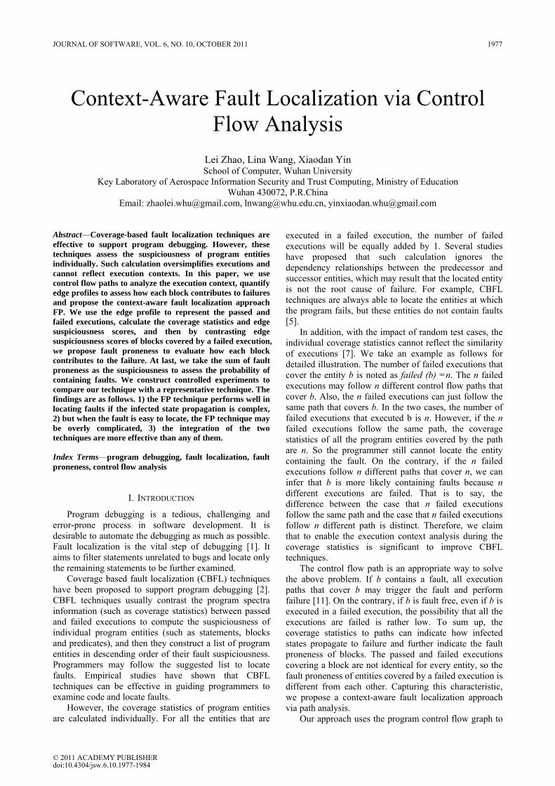
The experiments results are shown in Figure 3 and Figure 4. The results show the code inspection percentage on individual fault. The results shown in Figure 3 are used to express the effectiveness of our FP technique than Tarantula. However, the FP does not always perform well for every fault, that is, the effectiveness is not always better than Tarantula. We take results shown in Figure 4 for detailed analysis. First, we bring out the promising results.

Table 1 Statistics of Subject Programs

Program subjects No. of faults within different versions

No. of test cases

flex v1 v2 v3 v4 v5

567 19 20 17 16 9

grep v1 v2 v3 v4 v5

809 18 8 18 12 1

gzip v1 v2 v3 v4 v5

213 16 7 10 12 14



As shown is Figure 3, the x-axis refers to the serial numbers of faults of which the code inspection percentage is higher than 10% when Tarantula is employed, and the y-axis refers to the code inspection percentage to locate faults. If the length of the bar is shorter, the corresponding technique is more effective. The red bars represent the results of FP technique in this paper, and the blue bars refer to the results of Tarantula. From the results we can see that our results are promising when dealing with faults which are hard to be located with Tarantula method.

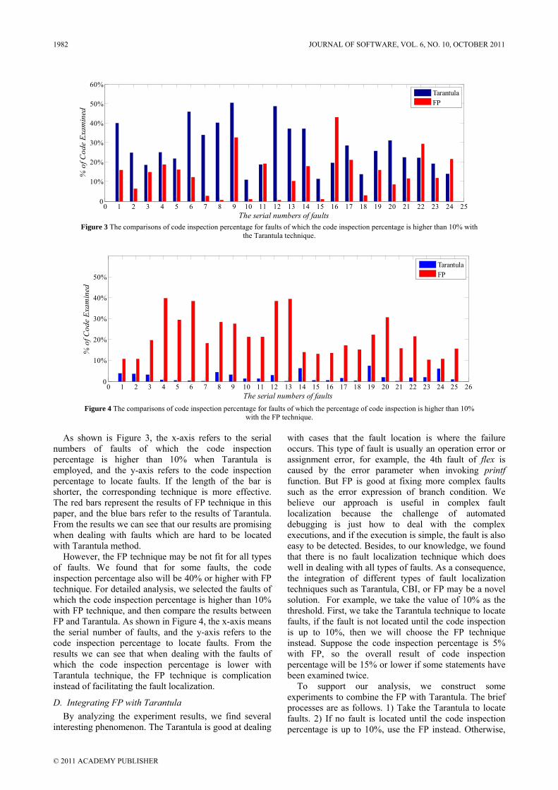
However, the FP technique may be not fit for all types of faults. We found that for some faults, the code inspection percentage also will be 40% or higher with FP technique. For detailed analysis, we selected the faults of which the code inspection percentage is higher than 10% with FP technique, and then compare the results between FP and Tarantula. As shown in Figure 4, the x-axis means the serial number of faults, and the y-axis refers to the code inspection percentage to locate faults. From the results we can see that when dealing with the faults of which the code inspection percentage is lower with Tarantula technique, the FP technique is complication instead of facilitating the fault localization.

D. Integrating FP with Tarantula By analyzing the experiment results, we find several

interesting phenomenon. The Tarantula is good at dealing

with cases that the fault location is where the failure occurs. This type of fault is usually an operation error or assignment error, for example, the 4th fault of flex is caused by the error parameter when invoking printf function. But FP is good at fixing more complex faults such as the error expression of branch condition. We believe our approach is useful in complex fault localization because the challenge of automated debugging is just how to deal with the complex executions, and if the execution is simple, the fault is also easy to be detected. Besides, to our knowledge, we found that there is no fault localization technique which does well in dealing with all types of faults. As a consequence, the integration of different types of fault localization techniques such as Tarantula, CBI, or FP may be a novel solution. For example, we take the value of 10% as the threshold. First, we take the Tarantula technique to locate faults, if the fault is not located until the code inspection is up to 10%, then we will choose the FP technique instead. Suppose the code inspection percentage is 5% with FP, so the overall result of code inspection percentage will be 15% or lower if some statements have been examined twice.

To support our analysis, we construct some experiments to combine the FP with Tarantula. The brief processes are as follows. 1) Take the Tarantula to locate faults. 2) If no fault is located until the code inspection percentage is up to 10%, use the FP instead. Otherwise,

0 1 2 3 4 5 6 7 8 9 10 11 12 13 14 15 16 17 18 19 20 21 22 23 24 250

10%

20%

30%

40%

50%

60%

The serial numbers of faults

% o

f Cod

e Ex

amin

ed

TarantulaFP

Figure 3 The comparisons of code inspection percentage for faults of which the code inspection percentage is higher than 10% with the Tarantula technique.

0 1 2 3 4 5 6 7 8 9 10 11 12 13 14 15 16 17 18 19 20 21 22 23 24 25 260

10%

20%

30%

40%

50%

The serial numbers of faults

% o

f Cod

e Ex

amin

ed

TarantulaFP

Figure 4 The comparisons of code inspection percentage for faults of which the percentage of code inspection is higher than 10% with the FP technique.



the process is end. 3) Locate the fault with FP technique until the fault is located. We take the sum of the code inspection percentage with two different techniques as the overall code inspection percentage.

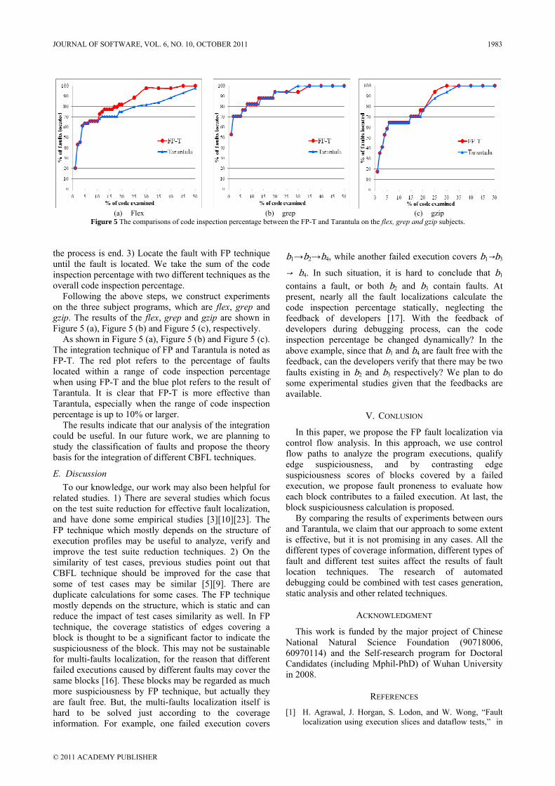
Following the above steps, we construct experiments on the three subject programs, which are flex, grep and gzip. The results of the flex, grep and gzip are shown in Figure 5 (a), Figure 5 (b) and Figure 5 (c), respectively.

As shown in Figure 5 (a), Figure 5 (b) and Figure 5 (c). The integration technique of FP and Tarantula is noted as FP-T. The red plot refers to the percentage of faults located within a range of code inspection percentage when using FP-T and the blue plot refers to the result of Tarantula. It is clear that FP-T is more effective than Tarantula, especially when the range of code inspection percentage is up to 10% or larger.

The results indicate that our analysis of the integration could be useful. In our future work, we are planning to study the classification of faults and propose the theory basis for the integration of different CBFL techniques.

E. Discussion To our knowledge, our work may also been helpful for

related studies. 1) There are several studies which focus on the test suite reduction for effective fault localization, and have done some empirical studies [3][10][23]. The FP technique which mostly depends on the structure of execution profiles may be useful to analyze, verify and improve the test suite reduction techniques. 2) On the similarity of test cases, previous studies point out that CBFL technique should be improved for the case that some of test cases may be similar [5][9]. There are duplicate calculations for some cases. The FP technique mostly depends on the structure, which is static and can reduce the impact of test cases similarity as well. In FP technique, the coverage statistics of edges covering a block is thought to be a significant factor to indicate the suspiciousness of the block. This may not be sustainable for multi-faults localization, for the reason that different failed executions caused by different faults may cover the same blocks [16]. These blocks may be regarded as much more suspiciousness by FP technique, but actually they are fault free. But, the multi-faults localization itself is hard to be solved just according to the coverage information. For example, one failed execution covers

b1→b2→b4, while another failed execution covers b1→b3

→ b4. In such situation, it is hard to conclude that b1 contains a fault, or both b2 and b3 contain faults. At present, nearly all the fault localizations calculate the code inspection percentage statically, neglecting the feedback of developers [17]. With the feedback of developers during debugging process, can the code inspection percentage be changed dynamically? In the above example, since that b1 and b4 are fault free with the feedback, can the developers verify that there may be two faults existing in b2 and b3 respectively? We plan to do some experimental studies given that the feedbacks are available.

V. CONLUSION

In this paper, we propose the FP fault localization via control flow analysis. In this approach, we use control flow paths to analyze the program executions, qualify edge suspiciousness, and by contrasting edge suspiciousness scores of blocks covered by a failed execution, we propose fault proneness to evaluate how each block contributes to a failed execution. At last, the block suspiciousness calculation is proposed.

By comparing the results of experiments between ours and Tarantula, we claim that our approach to some extent is effective, but it is not promising in any cases. All the different types of coverage information, different types of fault and different test suites affect the results of fault location techniques. The research of automated debugging could be combined with test cases generation, static analysis and other related techniques.

ACKNOWLEDGMENT

This work is funded by the major project of Chinese National Natural Science Foundation (90718006, 60970114) and the Self-research program for Doctoral Candidates (including Mphil-PhD) of Wuhan University in 2008.

REFERENCES

[1] H. Agrawal, J. Horgan, S. Lodon, and W. Wong, “Fault localization using execution slices and dataflow tests,” in

(a) Flex (b) grep (c) gzip

Figure 5 The comparisons of code inspection percentage between the FP-T and Tarantula on the flex, grep and gzip subjects.



Proceedings of the 6th International Symposium on Software Reliability Engineering, Toulouse, France, 1995, pp. 143–151.

[2] J. A. Jones and M. J. Harrold, “Empirical evaluation of the tarantula automatic fault-localization technique,” in Proceedings of the 20th IEEE International Conference on Automated Software Engineering (ASE 2005), Long Beach, California, 2005, pp. 273-282.

[3] Y. Yu, J. A. Jones, and M. J. Harrold, “An empirical study of the effects of test-suite reduction on fault localization,” in Proceedings of the 30th International Conference on Software Engineering (ICSE 2008), Leipzig, Germany, 2008, pp. 201-210.

[4] R. Santelices, J. A. Jones, Y. Yu, and M. J. Harrold, “Lightweight fault localization using multiple coverage types,” in Proceedings of the 31st International Conference on Software Engineering (ICSE 2009), Vancouver, Canada, 2009, pp. 56–66.

[5] E. Wong and Y. Qi, “Effective program debugging based on execution slices and inter-block data dependency,” Journal of Systems and Software, vol. 79, no. 2, 2006, pp. 891-903.

[6] Z. Zhang, W. K. Chan, and T. H. Tse, “Capturing propagation of infected program states,” in Proceedings of the 17th International Conference on Foundation of Software Engineering (FSE/ESEC 2009), Amsterdam, Nederland, 2009, pp. 43–52.

[7] E. Wong, Y. Qi, L. Zhao, and K. Cai, “Effective fault localization using code coverage,” in Proceedings of the 31st Annual International Computer Software and Application Conference (COMPSAC 2007), Beijing, China, 2007, pp. 449–456.

[8] L. Jiang and Z. Su, “Context-aware statistical debugging: from bug predictors to faulty control flow paths,” in Proceedings of the 22nd IEEE International Conference on Automated Software Engineering (ASE 2007), Atlanta, USA, 2007, pp. 184-193.

[9] D. Hao, L. Zhang, Y. Pan, H. Mei, and J. Sun, “On similarity-awareness in testing-based fault localization,” Journal of Automated Software Engineering, vol. 2008, no. 15, 2008, pp. 207–249.

[10] S. Artzi, J. Dolby, F. Tip, and M. Pistoia, “Directed test generation for effective fault localization,” in Proceedings of the 2010 Internet Symposium on Software Testing and Analysis (ISSTA 2010), Trento, Italy, 2010, pp. 49–59.

[11] J. Voas, “Pie: A dynamic failure-based technique,” IEEE Transaction on Software Engineering, vol. 18, no. 8, 1992, pp. 717-727.

[12] T. Chilimbi, B. Liblit, K. Mehra, and K. V. A. Nori, “Holmes: effective statistical debugging via efficient path profiling,” in Proceedings of the 31st International

Conference on Software Engineering (ICSE 2009), Vancouver, Canada, 2009, pp. 34–44.

[13] J. A. Jones and M. J. Harrold, “Visualization of test information to assist fault localization,” in Proceedings of the International Conference on Software Engineering (ICSE 2002), Orlando, USA, 2002, pp. 467–477.

[14] B. Liblit, A. Aiken, A. Zheng, and M. I. Jordan, “Bug isolation via remote program sampling,” in Proceedings of the ACM SIGPLAN 2003 Conference on Programming Language Design and Implementation (PLDI 2003), 2003, pp. 141–154.

[15] H. Do, S. G. Elbaum, and G. Rothermel, “Supporting controlled experimentation with testing techniques: an infrastructure and its potential impact,” Empirical Software Engineering, vol. 10, no. 4, 2005, pp. 405-435.

[16] C. Liu, X. Zhang, and J. Han, “A systematic study of failure proximity,” IEEE Transaction on Software Engineering, vol. 34, no. 6, pp. 826–843, 2008.

[17] D. Hao, L. Zhang, T. Xie, H. Mei, and J. Sun, “Interactive fault localization using test information,” Journal of Computer Science and Technology, vol. 24, no. 5, 2009, pp. 962–974.

[18] M. Renieris and S. Reiss, “Fault localization with nearest neighbor queries,” in Proceedings of the 18th IEEE International Conference on Automated Software Engineering (ASE 2003), Montreal, Canada, 2003, pp. 30–39.

[19] R. Abreu, P. Zoeteweij, and A. J. C. van Gemund, “On the accuracy of spectrum-based fault localization,” in Proceedings of the Testing: Academic and Industrial Conference, Practice and Research Techniques, 2007, pp. 89-98.

[20] B. Liblit, M. Naik, A. X. Zheng, A. Aiken, and M. I. Jordan, “Scalable statistical bug isolation,” in Proceedings of the ACM SIGPLAN 2005 Conference on Programming Language Design and Implementation (PLDI 2005), 2005, pp. 15-26.

[21] C. Liu, L. Fei, X. Yan, J. Han, and S. Midkiff, “Statistical debugging: a hypothesis testing-based approach,” IEEE Transaction on Software Engineering, vol. 32, no. 10, 2006, pp. 1-17.

[22] G. K. Baah, A. Podgurski, and M. J. Harrold, “The probabilistic program dependence graph and its application to fault diagnosis,” in Proceedings of the 2008 International Symposium on Software Testing and Analysis (ISSTA 2008), Seattle, WA, USA, 2008, pp. 189–208.

[23] B. Baudry, F. Fleurey, and Y. L. Traon, “Improving test suites for efficient fault localization,” in Proceedings of the 26th International Conference on Software Engineering (ICSE 2006), 2006, pp. 82–91.



context-aware fault localization via control flow analysis

Documents