context-aware power management · pdf filecontext-aware power management (capm), ... chapter 1...
TRANSCRIPT

Context-Aware Power Management
Colin Harris
A thesis submitted to the University of Dublin, Trinity College
in partial fulfillment of the requirements for the degree of
Doctor of Philosophy (Computer Science)
September 2006

Declaration
I, the undersigned, declare that this work has not previously been submitted to this or any other
University, and that unless otherwise stated, it is entirely my own work.
Colin Harris
Dated: 14th September 2006

Permission to Lend and/or Copy
I, the undersigned, agree that Trinity College Library may lend or copy this thesis upon request.
Colin Harris
Dated: 14th September 2006

Acknowledgements
I would like to sincerely thank my supervisor, Prof. Vinny Cahill, for all of his help, encouragement
and insights over the past four years. It has been an invaluable learning experience. I would also
like to thank the Irish Research Council for Science, Engineering and Technology who provided the
funding for this research.
To everyone who volunteered to take part in the user studies, I would like to say a huge thank
you for your openness and willingness to participate. I would particularly like to thank Dr. Myra
O’Regan for her help with the data analysis and Neil O’Connor for his assistance with the object-
range sensors. I would also like to thank the Department’s support staff for making everything run
so smoothly. In particular, Tom Kearney and the technicians for their help with the many hardware
issues.
A big thank you to all my colleagues in the Distributed Systems Group (DSG). It has been great
to be part of such a social group as DSG. I have fond memories of the canoe trips, the Chinese meals,
the coffee breaks and the friday football.
To my parents, brother and sisters, thank you for your support, love and friendship throughout
the years. Finally, thank you Helene for the love, patience and understanding you have shown during
the time it has taken to complete this research.
Colin Harris
University of Dublin, Trinity College
September 2006
iv

Abstract
With more and more computing devices being deployed in buildings there has been a steady rise in
buildings’ electricity consumption. These devices not only consume electricity but also produce heat,
which increases loading on ventilation systems, further increasing electricity consumption. At the
same time there is a pressing need to reduce overall building energy consumption. For example, the
European Union’s strategy for security of energy supply highlights energy saving in buildings as a
key target area. One approach to reducing energy consumption of devices in buildings is to improve
the effectiveness of their power management.
Current state-of-the-art computer power management is predominantly focused on extending bat-
tery life for mobile computing devices. The majority of policies are low-level and are used to manage
sub-components within the overall computing device. The key trade-off for these policies is device
performance versus increased battery life. In contrast, stationary computing devices do not have bat-
tery limitations and typically the most significant energy savings are achieved by switching the entire
device to standby. However, switching to a deep standby state can cause significant user annoyance
due to the relatively long resume time and possible false power downs. Consequently these energy
saving features are typically not enabled (or used with long timeouts). To increase enablement, poli-
cies for stationary devices need to operate in a near transparent fashion, i.e., operate automatically
and with little user-perceived performance degradation.
Context-aware pervasive computing describes a vision of computing everywhere that seamlessly
assists us in our daily tasks, i.e., many functions are intelligently automated. Information display,
computing, sensing and communication will be embedded in everyday objects and within the environ-
ment’s infrastructure. Seamless interaction with these devices will enable a person to focus on their
task at hand while the devices themselves vanish into the background. Realisation of this vision could
exacerbate the building energy problem as more stationary computing devices are deployed but it
could also provide a solution. Context information (e.g., user location information) likely to be avail-
able in such pervasive computing environments could enable highly effective power management for
v

many of a building’s electricity consuming devices. We term such power management techniques as
context-aware power management (CAPM), their principal objective being to minimise overall elec-
tricity consumption while maintaining user-perceived device performance. The current state of the
art in context-aware computing focuses on developing inference techniques for determining high-level
context from low-level, noisy, and incomplete sensor data. Possible approaches include rule-based
inference, Bayesian inference, fuzzy control, and hidden Markov models. Successful inference enables
the vision of computing services interfacing seamlessly and transparently with users’ daily tasks. One
such desirable, transparent service is context-aware power management.
We have identified several key requirements and designed a framework for CAPM. At the core
of the framework, a Bayesian inference technique is employed to infer relevant context from a given
range of sensors. We have identified the principal context required for effective CAPM as being (i)
when the user is not using and (ii) when the user is about to use a device. Accurately inferring
this user context is the most challenging part of CAPM. However, there is also a balance between
how much energy additional context can save and how much it will cost both monetarily and energy
wise. To date there has been some research in the area of CAPM but to our knowledge there has
been no detailed study as to what granularity of context is appropriate and what are the potential
energy savings.
We have conducted an extensive user study to empirically answer these questions for CAPM of
desktop PCs in an office environment. The sensors used are keyboard/mouse input, user presence
based on Bluetooth beaconing, near presence based on ultrasonic range detection, face detection, and
voice detection. Results from the study show that there is wide variability of usage patterns and
that there is a balance whereby adding more sensors actually increases the energy consumption. For
the desktop PC study, idle time, user presence, and near presence are sufficient for effective power
management coming within 6-9% of the theoretical optimal policy (on average). Beyond this face
detection and voice detection consumed more than they saved. The evaluation further demonstrates
the use of Bayesian inference as a viable technique for CAPM.
vi

Publications Related to this Ph.D.
[1] C. Harris and V. Cahill. Power Management for Stationary Machines in a Pervasive Com-
puting Environment. In 38th Annual Hawaii International Conference on System Sciences
(HICSS’2005). Hawaii Big Island, January 2005.
[2] C. Harris and V. Cahill. Exploiting User Behaviour for Context-Aware Power Management.
In International Conference On Wireless and Mobile Computing, Networking and Communica-
tions, Montreal, Canada, August 2005.
vii

Contents
Acknowledgements iv
Abstract iv
List of Tables xii
List of Figures xiii
List of Listings xvi
Chapter 1 Introduction 1
1.1 Motivation . . . . . . . . . . . . . . . . . . . . . . . . . . . . . . . . . . . . . . . . . . 1
1.2 Dynamic Power Management . . . . . . . . . . . . . . . . . . . . . . . . . . . . . . . . 7
1.3 Pervasive Computing . . . . . . . . . . . . . . . . . . . . . . . . . . . . . . . . . . . . . 8
1.4 Context-aware computing . . . . . . . . . . . . . . . . . . . . . . . . . . . . . . . . . . 10
1.5 Context-aware Power Management . . . . . . . . . . . . . . . . . . . . . . . . . . . . . 10
1.6 Thesis contribution . . . . . . . . . . . . . . . . . . . . . . . . . . . . . . . . . . . . . . 11
1.7 Road map . . . . . . . . . . . . . . . . . . . . . . . . . . . . . . . . . . . . . . . . . . . 12
Chapter 2 State of the Art 14
2.1 Dynamic power management . . . . . . . . . . . . . . . . . . . . . . . . . . . . . . . . 14
2.1.1 The oracle and threshold policies . . . . . . . . . . . . . . . . . . . . . . . . . . 17
2.2 Dynamic power management policies . . . . . . . . . . . . . . . . . . . . . . . . . . . . 19
2.2.1 Device-driver-level policies . . . . . . . . . . . . . . . . . . . . . . . . . . . . . . 20
2.2.2 Operating system-level policies . . . . . . . . . . . . . . . . . . . . . . . . . . . 22
2.2.3 Application-level policies . . . . . . . . . . . . . . . . . . . . . . . . . . . . . . 24
2.2.4 User-level policies . . . . . . . . . . . . . . . . . . . . . . . . . . . . . . . . . . 26
viii
2.2.5 Discussion . . . . . . . . . . . . . . . . . . . . . . . . . . . . . . . . . . . . . . 27
2.3 Context-aware computing . . . . . . . . . . . . . . . . . . . . . . . . . . . . . . . . . . 29
2.3.1 Context-aware computing model . . . . . . . . . . . . . . . . . . . . . . . . . . 29
2.3.2 Properties of sensors and multi-sensory information . . . . . . . . . . . . . . . 31
2.3.3 Granularity versus cost . . . . . . . . . . . . . . . . . . . . . . . . . . . . . . . 31
2.4 Context-aware power management review . . . . . . . . . . . . . . . . . . . . . . . . . 33
2.4.1 A context-aware approach to saving energy in wireless sensor networks . . . . . 33
2.4.1.1 Analysis . . . . . . . . . . . . . . . . . . . . . . . . . . . . . . . . . . 34
2.4.2 Location aware resource management in smart homes . . . . . . . . . . . . . . 34
2.4.2.1 Analysis . . . . . . . . . . . . . . . . . . . . . . . . . . . . . . . . . . 35
2.4.3 Improving home automation by discovering regularly occurring device usage
patterns . . . . . . . . . . . . . . . . . . . . . . . . . . . . . . . . . . . . . . . . 36
2.4.3.1 Analysis . . . . . . . . . . . . . . . . . . . . . . . . . . . . . . . . . . 38
2.4.4 An adaptive fuzzy learning mechanism for intelligent agents in ubiquitous com-
puting environments . . . . . . . . . . . . . . . . . . . . . . . . . . . . . . . . . 38
2.4.4.1 Analysis . . . . . . . . . . . . . . . . . . . . . . . . . . . . . . . . . . 40
2.4.5 Lessons from an Adaptive House . . . . . . . . . . . . . . . . . . . . . . . . . . 41
2.4.5.1 Analysis . . . . . . . . . . . . . . . . . . . . . . . . . . . . . . . . . . 43
2.5 User activity monitoring review . . . . . . . . . . . . . . . . . . . . . . . . . . . . . . . 44
2.5.1 Inferring Activities from Interactions with Objects . . . . . . . . . . . . . . . . 44
2.5.1.1 Analysis . . . . . . . . . . . . . . . . . . . . . . . . . . . . . . . . . . 46
2.5.2 Discovery and Segmentation of Activities in Video . . . . . . . . . . . . . . . . 47
2.5.2.1 Analysis . . . . . . . . . . . . . . . . . . . . . . . . . . . . . . . . . . 48
2.5.3 Layered Representations for Human Activity Recognition . . . . . . . . . . . . 49
2.5.3.1 Analysis . . . . . . . . . . . . . . . . . . . . . . . . . . . . . . . . . . 52
2.6 Summary . . . . . . . . . . . . . . . . . . . . . . . . . . . . . . . . . . . . . . . . . . . 53
Chapter 3 CAPM Framework Design 55
3.1 Initial experimental results . . . . . . . . . . . . . . . . . . . . . . . . . . . . . . . . . 55
3.1.1 SOB policy energy performance . . . . . . . . . . . . . . . . . . . . . . . . . . . 57
3.1.2 SOB policy user-perceived performance . . . . . . . . . . . . . . . . . . . . . . 58
3.1.3 SWOB policy energy performance . . . . . . . . . . . . . . . . . . . . . . . . . 59
3.1.4 SWOB user-perceived performance . . . . . . . . . . . . . . . . . . . . . . . . . 61
3.1.5 Conclusions . . . . . . . . . . . . . . . . . . . . . . . . . . . . . . . . . . . . . . 62
ix

3.2 CAPM requirements . . . . . . . . . . . . . . . . . . . . . . . . . . . . . . . . . . . . . 63
3.3 CAPM framework design . . . . . . . . . . . . . . . . . . . . . . . . . . . . . . . . . . 64
3.3.1 Data capture and feature extraction . . . . . . . . . . . . . . . . . . . . . . . . 65
3.3.2 Context inference . . . . . . . . . . . . . . . . . . . . . . . . . . . . . . . . . . . 66
3.3.3 Decision . . . . . . . . . . . . . . . . . . . . . . . . . . . . . . . . . . . . . . . . 66
3.4 Selection of inference technique . . . . . . . . . . . . . . . . . . . . . . . . . . . . . . . 66
3.5 Probability and Bayesian networks . . . . . . . . . . . . . . . . . . . . . . . . . . . . . 70
3.5.1 Bayesian networks . . . . . . . . . . . . . . . . . . . . . . . . . . . . . . . . . . 73
3.5.2 Dynamic Bayesian networks . . . . . . . . . . . . . . . . . . . . . . . . . . . . . 76
3.6 Parameter learning for Bayesian networks . . . . . . . . . . . . . . . . . . . . . . . . . 77
3.6.1 Parameter learning for binary variables . . . . . . . . . . . . . . . . . . . . . . 78
3.6.2 Learning multinomial variables . . . . . . . . . . . . . . . . . . . . . . . . . . . 80
3.7 Choice of sensors for CAPM . . . . . . . . . . . . . . . . . . . . . . . . . . . . . . . . . 81
3.8 Design of BNs for CAPM . . . . . . . . . . . . . . . . . . . . . . . . . . . . . . . . . . 82
3.8.1 Initial models . . . . . . . . . . . . . . . . . . . . . . . . . . . . . . . . . . . . . 82
3.8.1.1 Not using . . . . . . . . . . . . . . . . . . . . . . . . . . . . . . . . . . 82
3.8.1.2 About to use . . . . . . . . . . . . . . . . . . . . . . . . . . . . . . . . 84
3.8.2 Final BN models . . . . . . . . . . . . . . . . . . . . . . . . . . . . . . . . . . . 84
3.8.2.1 Not using . . . . . . . . . . . . . . . . . . . . . . . . . . . . . . . . . . 85
3.8.2.2 About to use . . . . . . . . . . . . . . . . . . . . . . . . . . . . . . . . 88
3.8.3 DBN models . . . . . . . . . . . . . . . . . . . . . . . . . . . . . . . . . . . . . 89
3.8.3.1 Not using . . . . . . . . . . . . . . . . . . . . . . . . . . . . . . . . . . 89
3.8.3.2 About to use . . . . . . . . . . . . . . . . . . . . . . . . . . . . . . . . 91
3.9 Summary . . . . . . . . . . . . . . . . . . . . . . . . . . . . . . . . . . . . . . . . . . . 91
Chapter 4 Implementation 93
4.1 Sensors . . . . . . . . . . . . . . . . . . . . . . . . . . . . . . . . . . . . . . . . . . . . 94
4.1.1 System idle time . . . . . . . . . . . . . . . . . . . . . . . . . . . . . . . . . . . 94
4.1.2 Bluetooth presence . . . . . . . . . . . . . . . . . . . . . . . . . . . . . . . . . . 96
4.1.3 Face detection . . . . . . . . . . . . . . . . . . . . . . . . . . . . . . . . . . . . 98
4.1.4 Voice activity detection . . . . . . . . . . . . . . . . . . . . . . . . . . . . . . . 100
4.1.5 Object range detection . . . . . . . . . . . . . . . . . . . . . . . . . . . . . . . . 102
4.1.6 Sensor power consumption . . . . . . . . . . . . . . . . . . . . . . . . . . . . . . 104
4.2 BN software selection . . . . . . . . . . . . . . . . . . . . . . . . . . . . . . . . . . . . 106
x

4.2.1 Requirements . . . . . . . . . . . . . . . . . . . . . . . . . . . . . . . . . . . . . 106
4.2.2 Tool selection . . . . . . . . . . . . . . . . . . . . . . . . . . . . . . . . . . . . 107
4.2.3 Netica . . . . . . . . . . . . . . . . . . . . . . . . . . . . . . . . . . . . . . . . . 108
4.3 Runtime (on-line) CAPM implementation . . . . . . . . . . . . . . . . . . . . . . . . . 109
4.4 Evaluation (off-line) CAPM implementation . . . . . . . . . . . . . . . . . . . . . . . . 111
4.4.1 Data collection . . . . . . . . . . . . . . . . . . . . . . . . . . . . . . . . . . . . 111
4.4.2 Simulation of policies . . . . . . . . . . . . . . . . . . . . . . . . . . . . . . . . 112
4.5 Summary . . . . . . . . . . . . . . . . . . . . . . . . . . . . . . . . . . . . . . . . . . . 113
Chapter 5 Evaluation 114
5.1 Objectives . . . . . . . . . . . . . . . . . . . . . . . . . . . . . . . . . . . . . . . . . . . 114
5.2 Design of the CAPM user study . . . . . . . . . . . . . . . . . . . . . . . . . . . . . . . 115
5.3 Data collection and processing . . . . . . . . . . . . . . . . . . . . . . . . . . . . . . . 117
5.4 Simulation of policy traces . . . . . . . . . . . . . . . . . . . . . . . . . . . . . . . . . . 118
5.5 Evaluation metrics . . . . . . . . . . . . . . . . . . . . . . . . . . . . . . . . . . . . . . 122
5.6 Results . . . . . . . . . . . . . . . . . . . . . . . . . . . . . . . . . . . . . . . . . . . . . 122
5.6.1 Oracle, SWOB, Always On and Threshold policies . . . . . . . . . . . . . . . . 123
5.6.2 Potential extra energy from SWOB . . . . . . . . . . . . . . . . . . . . . . . . . 126
5.6.3 Energy consumption of sensors . . . . . . . . . . . . . . . . . . . . . . . . . . . 127
5.6.4 BN models for power management of the display . . . . . . . . . . . . . . . . . 128
5.6.5 BN models for power management of the PC . . . . . . . . . . . . . . . . . . . 134
5.6.6 DBN models for power management of the display . . . . . . . . . . . . . . . . 138
5.6.7 DBN models for power management of the PC . . . . . . . . . . . . . . . . . . 138
5.7 Evaluation of the affect of monitoring on users . . . . . . . . . . . . . . . . . . . . . . 141
5.8 Evaluation of BNs for device power management . . . . . . . . . . . . . . . . . . . . . 143
5.9 Summary . . . . . . . . . . . . . . . . . . . . . . . . . . . . . . . . . . . . . . . . . . . 145
Chapter 6 Conclusions 147
6.1 Contribution . . . . . . . . . . . . . . . . . . . . . . . . . . . . . . . . . . . . . . . . . 147
6.2 Future work . . . . . . . . . . . . . . . . . . . . . . . . . . . . . . . . . . . . . . . . . . 149
Appendix A Additional Evaluation Figures 150
Bibliography 154
xi

List of Tables
1.1 Internal heat gains [68] . . . . . . . . . . . . . . . . . . . . . . . . . . . . . . . . . . . . 6
2.1 Power states, break-even and resume times . . . . . . . . . . . . . . . . . . . . . . . . 17
2.2 Measured power consumption of DELL Optiplex GX270 . . . . . . . . . . . . . . . . . 27
2.3 Average Scenario Prediction Results [27] . . . . . . . . . . . . . . . . . . . . . . . . . 37
2.4 Activities of daily living [52] . . . . . . . . . . . . . . . . . . . . . . . . . . . . . . . . . 45
2.5 Average accuracies and computational costs for S-SEER [49] . . . . . . . . . . . . . . 51
2.6 Recognition accuracy [50] . . . . . . . . . . . . . . . . . . . . . . . . . . . . . . . . . . 53
3.1 Joint probability table . . . . . . . . . . . . . . . . . . . . . . . . . . . . . . . . . . . . 74
3.2 Example BN training cases . . . . . . . . . . . . . . . . . . . . . . . . . . . . . . . . . 87
3.3 Example training cases for the DBN model . . . . . . . . . . . . . . . . . . . . . . . . 91
4.1 Comparison of BN tools . . . . . . . . . . . . . . . . . . . . . . . . . . . . . . . . . . . 107
5.1 Sample selection . . . . . . . . . . . . . . . . . . . . . . . . . . . . . . . . . . . . . . . 116
5.2 LightUse and HeavyUse users . . . . . . . . . . . . . . . . . . . . . . . . . . . . . . . . 123
xii

List of Figures
1.1 Residential and commercial energy consumption [14] . . . . . . . . . . . . . . . . . . . 2
1.2 Trinity College Dublin electricity consumption [15] . . . . . . . . . . . . . . . . . . . . 3
1.3 Unit energy cost and total energy cost per device type for USA [33] . . . . . . . . . . 4
1.4 Percentage energy cost per sector and per power state [33] . . . . . . . . . . . . . . . . 5
1.5 Cooling potential of ventilation for given internal/external delta temperature and ven-
tilation rate[68] . . . . . . . . . . . . . . . . . . . . . . . . . . . . . . . . . . . . . . . . 7
2.1 Usage periods and idle periods for a device . . . . . . . . . . . . . . . . . . . . . . . . 15
2.2 Dynamically power managed device . . . . . . . . . . . . . . . . . . . . . . . . . . . . 16
2.3 The theoretically optimal oracle policy . . . . . . . . . . . . . . . . . . . . . . . . . . . 18
2.4 Trade off power consumption versus performance . . . . . . . . . . . . . . . . . . . . . 18
2.5 Device-level power management . . . . . . . . . . . . . . . . . . . . . . . . . . . . . . . 20
2.6 Operating system-level power management . . . . . . . . . . . . . . . . . . . . . . . . 23
2.7 Application-level power management . . . . . . . . . . . . . . . . . . . . . . . . . . . . 25
2.8 User-level power management . . . . . . . . . . . . . . . . . . . . . . . . . . . . . . . . 26
2.9 Sentient object model . . . . . . . . . . . . . . . . . . . . . . . . . . . . . . . . . . . . 30
2.10 MavHome floor plan . . . . . . . . . . . . . . . . . . . . . . . . . . . . . . . . . . . . . 35
2.11 Five phases of AOFIS [19] . . . . . . . . . . . . . . . . . . . . . . . . . . . . . . . . . 39
2.12 Rule modifications [19] . . . . . . . . . . . . . . . . . . . . . . . . . . . . . . . . . . . 40
2.13 Adaptive House Architecture (ACHE)[43] . . . . . . . . . . . . . . . . . . . . . . . . . 42
2.14 Energy versus user discomfort [43] . . . . . . . . . . . . . . . . . . . . . . . . . . . . . 43
2.15 Several learned states in the trained HMM model. (a) entering room, (b) at com-
puter, (c) at white board, (d) sitting, (e) on telephone, (f) looking for a
key, (g) writing, and (h) swiveling right. [7] . . . . . . . . . . . . . . . . . . . . 48
2.16 S-SEER dynamic Bayesian network [50] . . . . . . . . . . . . . . . . . . . . . . . . . . 52
xiii

3.1 SOB energy consumption . . . . . . . . . . . . . . . . . . . . . . . . . . . . . . . . . . 57
3.2 SOB user performance . . . . . . . . . . . . . . . . . . . . . . . . . . . . . . . . . . . . 59
3.3 Standby period frequency . . . . . . . . . . . . . . . . . . . . . . . . . . . . . . . . . . 59
3.4 SWOB energy consumption . . . . . . . . . . . . . . . . . . . . . . . . . . . . . . . . . 60
3.5 Auto-on-idle period frequency in seconds . . . . . . . . . . . . . . . . . . . . . . . . . . 61
3.6 Standby period frequencies (minutes) . . . . . . . . . . . . . . . . . . . . . . . . . . . . 63
3.7 CAPM framework . . . . . . . . . . . . . . . . . . . . . . . . . . . . . . . . . . . . . . 65
3.8 Venn diagram showing conditional probability . . . . . . . . . . . . . . . . . . . . . . . 72
3.9 BN example . . . . . . . . . . . . . . . . . . . . . . . . . . . . . . . . . . . . . . . . . . 73
3.10 Example BN for ubiquitous computing . . . . . . . . . . . . . . . . . . . . . . . . . . . 76
3.11 Example DBN rolled out to 3 time slices . . . . . . . . . . . . . . . . . . . . . . . . . . 77
3.12 Augmented Bayesian network . . . . . . . . . . . . . . . . . . . . . . . . . . . . . . . . 78
3.13 Beta distributions . . . . . . . . . . . . . . . . . . . . . . . . . . . . . . . . . . . . . . 79
3.14 Updating the Beta distribution . . . . . . . . . . . . . . . . . . . . . . . . . . . . . . . 80
3.15 Initial not using model . . . . . . . . . . . . . . . . . . . . . . . . . . . . . . . . . . . 83
3.16 Initial about to use model . . . . . . . . . . . . . . . . . . . . . . . . . . . . . . . . 84
3.17 Final BN not using model . . . . . . . . . . . . . . . . . . . . . . . . . . . . . . . . . 85
3.18 Final BN about to use model . . . . . . . . . . . . . . . . . . . . . . . . . . . . . . . 89
3.19 DBN not using model . . . . . . . . . . . . . . . . . . . . . . . . . . . . . . . . . . . 90
4.1 Software structure . . . . . . . . . . . . . . . . . . . . . . . . . . . . . . . . . . . . . . 93
4.2 Idle time CPTs . . . . . . . . . . . . . . . . . . . . . . . . . . . . . . . . . . . . . . . . 95
4.3 Inferred probability of not using . . . . . . . . . . . . . . . . . . . . . . . . . . . . . 95
4.4 Bluetooth CPTs . . . . . . . . . . . . . . . . . . . . . . . . . . . . . . . . . . . . . . . 97
4.5 Inferred probability of not using . . . . . . . . . . . . . . . . . . . . . . . . . . . . . 97
4.6 The Haar-like features . . . . . . . . . . . . . . . . . . . . . . . . . . . . . . . . . . . . 99
4.7 Face detection . . . . . . . . . . . . . . . . . . . . . . . . . . . . . . . . . . . . . . . . . 100
4.8 Face detection CPTs . . . . . . . . . . . . . . . . . . . . . . . . . . . . . . . . . . . . . 101
4.9 Voice activity CPTs . . . . . . . . . . . . . . . . . . . . . . . . . . . . . . . . . . . . . 102
4.10 Typical using/not using object ranges . . . . . . . . . . . . . . . . . . . . . . . . . . 103
4.11 Coinciding using/not using object ranges . . . . . . . . . . . . . . . . . . . . . . . . 104
4.12 Object detection CPTs . . . . . . . . . . . . . . . . . . . . . . . . . . . . . . . . . . . . 104
4.13 Energy consumption of sensors . . . . . . . . . . . . . . . . . . . . . . . . . . . . . . . 105
4.14 Evaluation software structure . . . . . . . . . . . . . . . . . . . . . . . . . . . . . . . . 111
xiv

4.15 Device Model . . . . . . . . . . . . . . . . . . . . . . . . . . . . . . . . . . . . . . . . . 112
4.16 CAPM simluation . . . . . . . . . . . . . . . . . . . . . . . . . . . . . . . . . . . . . . 113
5.1 Measured device usage . . . . . . . . . . . . . . . . . . . . . . . . . . . . . . . . . . . . 118
5.2 Oracle versus Measured . . . . . . . . . . . . . . . . . . . . . . . . . . . . . . . . . . . 119
5.3 SWOB versus Measured . . . . . . . . . . . . . . . . . . . . . . . . . . . . . . . . . . . 120
5.4 Threshold 5 versus Measured . . . . . . . . . . . . . . . . . . . . . . . . . . . . . . . . 120
5.5 BN IT-BT versus Measured . . . . . . . . . . . . . . . . . . . . . . . . . . . . . . . . . 121
5.6 SWOB total energy comparison . . . . . . . . . . . . . . . . . . . . . . . . . . . . . . . 125
5.7 False power downs per day . . . . . . . . . . . . . . . . . . . . . . . . . . . . . . . . . 126
5.8 Manual power ups . . . . . . . . . . . . . . . . . . . . . . . . . . . . . . . . . . . . . . 126
5.9 Potential extra energy from SWOB . . . . . . . . . . . . . . . . . . . . . . . . . . . . . 127
5.10 Estimated sensor energy consumption per day . . . . . . . . . . . . . . . . . . . . . . . 128
5.11 Delta energy . . . . . . . . . . . . . . . . . . . . . . . . . . . . . . . . . . . . . . . . . 130
5.12 Delta energy including sensor energy . . . . . . . . . . . . . . . . . . . . . . . . . . . . 131
5.13 False power downs . . . . . . . . . . . . . . . . . . . . . . . . . . . . . . . . . . . . . . 132
5.14 Manual power ups . . . . . . . . . . . . . . . . . . . . . . . . . . . . . . . . . . . . . . 132
5.15 Standby break-even periods . . . . . . . . . . . . . . . . . . . . . . . . . . . . . . . . . 133
5.16 Delta energy including sensor energy . . . . . . . . . . . . . . . . . . . . . . . . . . . . 135
5.17 False power downs . . . . . . . . . . . . . . . . . . . . . . . . . . . . . . . . . . . . . . 136
5.18 Manual power ups . . . . . . . . . . . . . . . . . . . . . . . . . . . . . . . . . . . . . . 136
5.19 Standby break-evens . . . . . . . . . . . . . . . . . . . . . . . . . . . . . . . . . . . . . 137
5.20 DBN display delta energy including sensor energy . . . . . . . . . . . . . . . . . . . . . 139
5.21 DBN PC delta energy including sensor energy . . . . . . . . . . . . . . . . . . . . . . . 140
5.22 Example DBN policy trace . . . . . . . . . . . . . . . . . . . . . . . . . . . . . . . . . 141
5.23 Idle traces for 6 of the users . . . . . . . . . . . . . . . . . . . . . . . . . . . . . . . . . 142
5.24 Bluetooth parameters given the user is not using . . . . . . . . . . . . . . . . . . . . 143
5.25 Variance in BT parameters for the 5 training days . . . . . . . . . . . . . . . . . . . . 144
5.26 Variance in energy consumption per training day . . . . . . . . . . . . . . . . . . . . . 145
A.1 DBN display false power downs . . . . . . . . . . . . . . . . . . . . . . . . . . . . . . . 151
A.2 DBN display manual power ups . . . . . . . . . . . . . . . . . . . . . . . . . . . . . . . 151
A.3 DBN display standby break-evens . . . . . . . . . . . . . . . . . . . . . . . . . . . . . . 152
A.4 DBN PC false power downs . . . . . . . . . . . . . . . . . . . . . . . . . . . . . . . . . 152
xv

A.5 DBN PC manual power ups . . . . . . . . . . . . . . . . . . . . . . . . . . . . . . . . . 153
A.6 DBN PC standby break-evens . . . . . . . . . . . . . . . . . . . . . . . . . . . . . . . . 153
xvi

Listings
4.1 System idle time . . . . . . . . . . . . . . . . . . . . . . . . . . . . . . . . . . . . . . . 94
4.2 CAPM . . . . . . . . . . . . . . . . . . . . . . . . . . . . . . . . . . . . . . . . . . . . . 110
xvii

Chapter 1
Introduction
This thesis investigates the potential for context information (e.g., user location information), likely
to be available in future pervasive computing environments, to enable highly effective device power
management. The principal objective of such context-aware power management (CAPM) is to min-
imise the overall electricity consumption of an environment’s stationary devices, while maintaining
acceptable user-perceived device performance. Secondary benefits are reduced noise and heat gain.
The thesis focuses on a future pervasive computing office environment containing sensing devices
such as location tags, imaging, audio, object detection, and stationary devices such as video displays,
desktop PCs, printers, photocopiers, ventilation, and lighting.
1.1 Motivation
The European Union (EU) strategy for security of energy supply [13] highlights three main issues:
1. The EU will become increasingly dependent on external energy sources; enlargement will rein-
force this trend. Based on current forecasts, if measures are not taken, import dependence will
reach 70% of total energy consumption in 2030, compared to 50% today.
2. At present, greenhouse gas emissions in the EU are on the rise, making it difficult to respond to
the challenge of climate change and to meet the EU’s commitments under the Kyoto protocol
[45].
3. The EU has very limited scope to influence energy supply conditions. It is essentially on the
demand side that the EU can intervene, mainly by promoting energy savings in buildings and
in the transport sector.
1

Cooking7%
Lighting & Appliances11%
Water heating25%
Space heating57%
Cooking5%
Lighting14%
Water heating9%
Space heating52%
Cooling4%
Other (mainly office equipment)
16%
Figure 1.1: Residential and commercial energy consumption [14]
The EU’s demand for energy has been growing at a rate of between 1% and 2% a year since 1986.
While industrial demand has remained stable, households and the tertiary sector have increased their
demand for electricity, transport, and heat. In particular demand for electricity has grown much more
rapidly than any other type of energy and is predicted to track gross domestic product (GDP) growth
closely until 2020 [13]. The total energy consumption of the EU in 1997 was estimated at 10,815 Tera-
Watt hours (TWh). Of this total, 40% was used in the building sector and 32% in the transport
sector [14]. Within the building sector residential properties consume 70% and commercial buildings
consume 30%. Figure 1.1 shows the breakdown of how energy is consumed in both residential and
commercial buildings.
The charts show that commercial buildings consume slightly less energy for heating but signifi-
cantly more energy for lighting and other uses (mainly office equipment and building services’ pumps
and fans at about 8% each [47]). The current trend is that while buildings are gradually becoming
better insulated reducing heat demand, increasing demand for appliances and services often offset
heating efficiency gains. Furthermore, improved energy efficiency in electrical devices (e.g., energy
saving light bulbs, and flat-screen monitors) has been more than offset by growing demand.
We conducted an analysis of electrical energy consumption for all buildings within Trinity College
to compare with the estimates and trends above1. The stock of office equipment operating within
the university was estimated from asset registers, sales records and network addresses for the year
2003. Multiplying the number of devices by their corresponding unit energy cost (UEC) (see Figure
1.3 below) gives a total energy cost (TEC) of around 0.003 TWh for office equipment within the
university for 2003. This equates to 14.7% of the College’s total electricity consumption or around1The analysis was conducted as part of an EU pilot action for procurement of energy-efficient office equipment [15].
2

0
2000
4000
6000
8000
10000
12000
14000
16000
18000
20000
95-96 96-97 97-98 98-99 99-00 00-01
Electricity (MWh) Students Building area (10m2) Desktop PCs
Figure 1.2: Trinity College Dublin electricity consumption [15]
euro 190,000 in financial cost. Figure 1.2 shows electricity consumption, student numbers, building
area and number of desktop PCs from 1995 to 2001. Electricity consumption has increased by over
50% in this period outstripping the increase in students and building area. At the same time the
number of desktop PCs increased by 800%.
Part of this trend of increased electrical energy consumption in buildings is due to the increased
numbers of computing devices (office equipment) being deployed in buildings. The Lawerence Berkeley
National Laboratory (LBNL) provides detailed estimates of energy consumed by office and network
equipment in the United States as of 1999 [33]. The office equipment is divided into 11 types of
device and categorised into residential and non-residential sectors as usage varies between the sectors.
Figure 1.3 details the estimated unit energy cost and total energy cost for each device type over a
period of a year for both the residential and non-residential sectors. UEC is charted in kilo-Watt
hours per year (kWh/year) and the scale is logarithmic to include the minicomputer and mainframe
devices which consume 5,840 and 58,400 kWh/year respectively.
The UEC figures are multiplied by the estimated number of devices existing in the residential and
non-residential sectors to give the total energy cost for each device type in TWh/year. The charts
highlight that even though the unit energy cost of the minicomputer and mainframe far exceed other
office equipment, both the desktop computer and the desktop display unit have the two highest total
energy costs, due to the shear number of them (estimated 109,110 desktop computers and 109,180
displays in the USA in 1999 compared to 2,020 minicomputers and 107 mainframes). The total energy
3

1
10
100
1000
10000
100000
1000000
Porta
ble co
mpu
ter
Desto
p com
puter
Serve
r
Minico
mpu
ter
Mainfram
e
Term
inal
Display
Lase
r prin
ter
Inkje
t prin
ter
Copie
rFax
kWh/
year
Residential
Non-residential
(a) Annual unit energy cost per device type (kWh/year)
0
2
4
6
8
10
12
14
Porta
ble co
mpu
ter
Desto
p com
puter
Serve
r
Minico
mpu
ter
Mainfram
e
Term
inal
Display
Lase
r prin
ter
Inkje
t prin
ter
Copie
rFax
TWh/
year
Residential
Non-residential
(b) Annual total energy cost per device type (TWh/year)
Figure 1.3: Unit energy cost and total energy cost per device type for USA [33]
4

Soft-off3.8% Low-power
standby8.6%
Operating86.3%
Printing or copying1.3%
Network4.3%
Residential11.7%
Non-residential84.0%
Figure 1.4: Percentage energy cost per sector and per power state [33]
cost of network equipment is estimated to be 3.22 TWh/year, which includes routers, switches, access
devices and hubs for wide area and local area networks.
Breaking down the energy cost per sector shows clearly that non-residential is the main energy
consumer for office equipment and breaking down into device power states shows that the majority
of energy is consumed by devices during their operating state (see Figure 1.4). The study took
a simplified model of device power states assuming that each device has one operating state, one
low-power standby state, and a soft-off state (many electrical devices still consume energy when
physically switched off and still connected to the mains). The printing or copying state models the
power consumed by devices when they are printing or copying2. Furthermore, LBNL note that the
main potential for savings due to power management are in displays, desktop computers, and copiers,
which currently have low enablement of their power management features (estimated to be about
25% enabled).
Another reason for increased electrical energy consumption in buildings is the increased deploy-
ment of air conditioning and mechanical ventilation (fans) to cool building environments during the
summer months. The increasing numbers of computing devices adds to ventilation loading, which
further increases electricity consumption. Roughly speaking the heat energy dissipated from a device
is equivalent to its energy consumption. So, a 45 Watt (W) LCD display will dissipate about 45 W
of heat energy and a 60 W desktop computer will dissipate around 60 W of heat. An air conditioned
space with a 200% efficiency will consume 52.5 W to dissipate the heat from the one display and2The power consumed when printing or copying is significantly higher than in the normal operating state.
5

desktop computer.
Natural ventilation is an alternative technique that maximises use of windows and natural airflows
to passively ventilate and cool the environment, significantly reducing energy consumption for cooling
and ventilation. Natural ventilation is particularly suited to temperate climates which have moderate
temperature variations throughout the year. Given a suitable climate, the principal factor in the
viability of natural ventilation is the heat gain in the space. The primary internal heat sources are
people, lighting, and small power devices (e.g., office equipment). Table 1.1 gives figures for typical
internal heat gains in an office environment for low, medium and high densities of the three factors.
Gains (W/m2) Low Medium High
People 5-8 8-11 11-15
Lights 3-5 6-9 10-14
Small power 0-6 6-12 12-20
Total 6-16 18-30 30-50
Table 1.1: Internal heat gains [68]
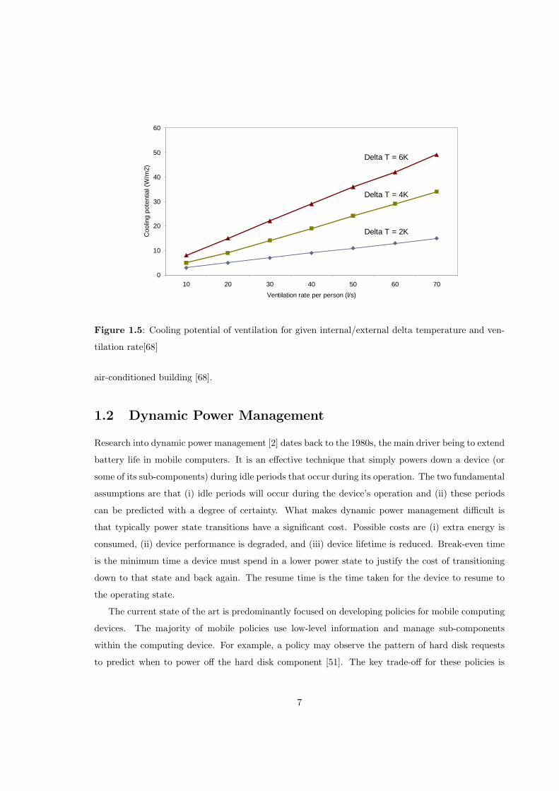
For overheating to be controlled by ventilation, there is a limit to the allowable heat gains within
the space. This is because the cooling energy coming from the cooler external air is not controllable
and the thermal mass of the building (which at night time stores the cooling energy) is limited. Figure
1.5 shows the cooling potential of ventilation for given internal/external temperature difference (Delta
T) and ventilation rates in litres per second per person (l/s/p). Typical high-density internal heat
gains from Table 1.1 range from 30 to 50 W/m2. The ECON19 benchmark [47] specifies a target
energy efficient mechanical ventilation rate for cooling of 40 l/s/p. From the figure it can be seen
that 30 W/m2 cooling would be just achievable for the night time 6 degree temperature difference
but no where near achievable for a typical day time 2 degree temperature difference.
In summary, we believe that effective device power management will provide several significant
benefits for both the operators and users of commercial buildings. It will contribute to significant
energy savings in lighting and appliances (22% of commercial building energy) and it will reduce the
need for air conditioned and mechanically ventilated spaces significantly reducing energy consumed
by ventilation and cooling (12% of commercial building energy). For the users, it will enable a
more pleasant working environment with more naturally ventilated spaces and reduced noise levels
through less need for mechanical fans and air-conditioning units and more computing devices in silent
standby modes. Many example building projects cite building users wanting a more user friendly
“open” building where they can open windows to control their environment as opposed to their sealed
6
0
10
20
30
40
50
60
10 20 30 40 50 60 70
Ventilation rate per person (l/s)
Coo
ling
pote
ntia
l (W
/m2)
Delta T = 6K
Delta T = 4K
Delta T = 2K
Figure 1.5: Cooling potential of ventilation for given internal/external delta temperature and ven-
tilation rate[68]
air-conditioned building [68].
1.2 Dynamic Power Management
Research into dynamic power management [2] dates back to the 1980s, the main driver being to extend
battery life in mobile computers. It is an effective technique that simply powers down a device (or
some of its sub-components) during idle periods that occur during its operation. The two fundamental
assumptions are that (i) idle periods will occur during the device’s operation and (ii) these periods
can be predicted with a degree of certainty. What makes dynamic power management difficult is
that typically power state transitions have a significant cost. Possible costs are (i) extra energy is
consumed, (ii) device performance is degraded, and (iii) device lifetime is reduced. Break-even time
is the minimum time a device must spend in a lower power state to justify the cost of transitioning
down to that state and back again. The resume time is the time taken for the device to resume to
the operating state.
The current state of the art is predominantly focused on developing policies for mobile computing
devices. The majority of mobile policies use low-level information and manage sub-components
within the computing device. For example, a policy may observe the pattern of hard disk requests
to predict when to power off the hard disk component [51]. The key trade-off for these policies is
7

device performance versus increased battery life. The hard disk may be aggressively power managed
to extend battery life but its performance will deteriorate as it will be slower to respond to user
requests. These low-level mobile policies can only predict short idle periods and are not able to
predict the time of the next user request, hence they incur a performance delay the next time the
user requests the device. Therefore, they are only suitable for managing devices or sub-components
which have relatively short break-even and resume times (order 10 and 1 seconds respectively [20]).
Typically, the most significant power savings for stationary devices are achieved by switching
the entire device to standby. However, switching to a deep standby state has two implications as the
device break-even and resume times are significantly longer. Firstly, since break-even times are longer,
policies need to accurately predict longer idle periods (order 1 to 10 minutes). Second, switching to
low-power standby states can cause significant user annoyance as resume times are longer (order 10
seconds) and there is the possibility of false power downs. Furthermore, stationary computing devices
do not have battery limitations so users expect little or no performance degradation. Therefore,
policies need to be near certain before powering down and they need to predict the time of the next
user request to avoid resume time delays.
Currently, the standard policy for power managing stationary devices is the threshold policy, which
simply waits a certain threshold period of idleness before powering down the device. It is neither able
to predict long idle periods nor the time of the next user request. As a result of these inadequacies
deeper standby energy saving features are typically not enabled (or set to a long timeout). To increase
enablement of these features, policies for stationary devices need to operate in a near transparent
fashion (i.e., operate automatically with little user-perceived performance degradation).
1.3 Pervasive Computing
Pervasive or ubiquitous computing is heralded as the next stage in the evolution of computing [66, 58].
Instead of today’s situation where people use dedicated computing devices (e.g., desktop computers)
to access information and perform their“computing”tasks, pervasive computing envisions information
display, computing, sensing, and communication existing all around, embedded in everyday objects
and the environment’s infrastructure3. The objective of this being to assist people with their everyday
tasks by providing information, computing, and services in an “intelligent”, seamless manner. This
seamless integration enables people to focus on their task at hand while the computers themselves
vanish into the background. They need not be explicitly aware of the computing devices involved3We view smart spaces as a subset of pervasive computing which deals specifically with adding “intelligence” to
building environments.
8

in their daily tasks and so the computing becomes transparent. The vision relies on the availability
of cheap computing, communication, sensing, and display devices pervasively deployed within the
environment and the ability to “intelligently” integrate services with users’ everyday tasks.
We are already seeing the beginnings of the vision today with the almost saturated deployment
of mobile phones (many with significant computing capability) and many shops and public buildings
using large video displays to display information. There are also many embedded computing devices
in everyday objects such as home appliances, cars, and street furniture (e.g., bus stops). What still
has to be achieved is the seamless interaction of all these devices to provide users with useful services
in a transparent manner.
However, realisation of this pervasive computing vision could exacerbate the building energy
problem as more computing, communication, sensing, and display devices are deployed in buildings.
Weiser [66] considers the type of devices that might become common in a typical office environment.
He cites one issue of crucial importance being scale. Devices will come in different sizes, each suited
to a particular task. The devices he experimented with are tabs (post-it note size), pads (A4 paper
size), and boards (bulletin board size). He envisaged a typical office containing more than 100 tabs,
10 to 20 pads and one or two boards. The tabs and pads are battery powered requiring recharging
periodically while the boards are stationary. The boards can serve a number of functions such as
bulletin boards for displaying information, white boards for collaboration in a meeting and electronic
bookcases from which a user might download some information to their pad or tab. Satyanaraynan [58]
envisions public spaces augmented with“surrogate” servers to provide computing service for handheld
device users. Increasing numbers of these stationary devices are a real concern for increasing energy
consumption in buildings. Furthermore, Jain [31] cites energy consumption due to mobile devices
as a significant environmental concern for pervasive computing. “While mobile devices are becoming
more energy efficient, the overall energy consumption due to such devices continues to increase as
their total number increases rapidly.”
These are well-founded concerns for pervasive computing. However, on the other hand pervasive
computing could possibly provide a solution by enabling more“intelligent”device power management.
For example, user location information, likely to be available in pervasive computing environments
could enable highly effective power management for many of a building’s electricity consuming devices.
We have termed such techniques that make use of “context” as context-aware power management
(CAPM) [26]. It is enabled by research being carried out in the areas of dynamic power management
and context-aware computing.
9

1.4 Context-aware computing
Context-aware computing is one of the fundamental components in realising the pervasive computing
vision. Context describes the state of the environment in which an application operates and the state
of the user (or users). In general, context typically consists of location, identity, user activity, envi-
ronmental properties, and available resources [3]. Being context-aware can be defined as the ability
to sense and react to context, enabling autonomous, proactive operation by reducing or eliminating
the need for explicit user input to the application.
Satyanarayanan [58] describes a scenario for this proactive, seamless context-aware computing.
“Fred is preparing a presentation on his desktop PC. Being late for the meeting he grabs his handheld
PC and leaves the office. The presentation is automatically transferred to the handheld so he can
continue editing while walking across campus to the meeting. The system infers Fred is going to
the meeting from his calendar information and the location tracking service. Before entering the
meeting the presentation is downloaded to the projection PC and the projector is switched on to
warm up. During the presentation face detection cameras in the room detect unfamiliar people, the
system warns Fred not to present a slide which contains sensitive information.” The scenario shows
things being seamlessly/proactively automated for the user, downloading the presentation, switching
on the projector, warning Fred not to present a sensitive slide. They all require the system to be
context-aware, aware of the state of the environment and what the user is doing or going to do.
The current state of the art in context-aware computing focuses on developing inference techniques
for determining high-level contexts from low-level, noisy, and incomplete sensor data. Possible ap-
proaches include rule-based inference, Bayesian networks, fuzzy control, and hidden Markov models
[56]. Successful inference enables the vision of computing services interfacing seamlessly with users’
daily tasks. One such useful, transparent service is context-aware power management.
1.5 Context-aware Power Management
We define context-aware power management as a dynamic power management technique that employs
high-level user context to transparently power manage users’ devices. It is possible to apply CAPM
to manage users’ mobile devices but this thesis focuses on the management of stationary devices, the
principal objective being to minimise overall electricity consumption while maintaining user-perceived
device performance.
In imagining an ideal CAPM scenario, all electricity consuming devices are instantly switched to
very low-power standby states when not in use and these devices are restored to their operating states
10

just before the user requests their service again. To develop effective CAPM policies that approach
this ideal we need to obtain context from the user of the device. We identify the key context to infer
as (i) when the user is not using the device (for the break-even period) and (ii) when the user is
about to use the device (at least the resume time beforehand). Determining this user context is the
most challenging part of context-aware power management. However, there is also a balance between
how much energy additional context can save and how much it will cost both monetarily and energy
wise.
We state that it is necessary to investigate what granularity of context is appropriate for CAPM.
Intuitively, finer-grained context can be obtained by adding more and different types of sensor into
the space. Observing additional features enables detection of more distinct patterns/cues for finer-
grained context. Subsequently, this more precise information enables policies to make better and
more timely decisions. However, also intuitively, the more hardware sensors there are and the more
feature processing, the more energy will be consumed by the policies. In carrying out this research
we are trying to discover what types of sensor are useful for CAPM, what are the benefits of adding
the sensors and what are the costs. In particular, is there a linear relationship between granularity of
sensors and energy saving or are there “sweet spots” where certain types of sensor give near optimal
performance for little additional cost. It is possible to leverage some context already available in the
pervasive environment such as estimated user location from wireless connections, but in some cases
it is necessary to include CAPM-specific sensors to obtain optimal performance.
Finally, the ground work for CAPM is being laid by advances in power management functionality
for computing devices. The advanced configuration and power interface (ACPI) [28] is a de facto
standard aimed at enabling effective power management for computing devices. The designers of the
standard and PC manufacturers have worked successfully towards achieving very low-power standby
states and faster resume times for their computing products. Also, moving the power management
code from the BIOS4 into the operating system has dealt with a number of reliability issues making
power management more robust [34]. Work is still on going in achieving even lower power states,
faster resume times and more robust operation. This will further increase the potential of CAPM.
1.6 Thesis contribution
To date there has been some research in the area of context-aware power management but to our
knowledge there has been no detailed study as to what are the potential energy savings from CAPM4The previous advanced power management (APM) standard was implemented in the BIOS.
11

and what granularity of context is appropriate. The main contribution of our research is to evaluate
the potential for context-aware power management within pervasive computing environments. In
particular we:
1. Identify requirements for CAPM and what context is useful for CAPM.
2. Design and implement a framework for CAPM.
3. Evaluate the potential of CAPM, in particular:
(a) What are the potential energy savings of using additional sensors?
(b) How good a cue are they for predicting the contexts not using and about to use?
(c) What is the estimated energy cost of the sensor hardware and data processing?
4. Evaluate Bayesian networks as a technique for implementing CAPM. In particular we evaluate
the performance of Bayesian networks with that of dynamic Bayesian networks.
5. Provide recommendations for a reasonable approach to CAPM.
We have conducted an extensive user study to empirically answer these questions for CAPM of desktop
PCs in an office environment. At the core of the CAPM framework, a Bayesian inference technique
is employed to infer relevant context from a range of sensors (user input, Bluetooth beaconing,
ultrasonic range detection, face detection, and voice detection). Results from the study show that
there is wide variability of usage patterns and that there is a balance whereby adding more sensors
actually increases energy consumption. For the desktop PC study, idle time, presence, and near
presence are sufficient for effective power management coming within 6-9% of the theoretical optimal
policy (on average). Beyond this, face detection and voice detection consumed more than they saved.
Finally, the evaluation showed that use dynamic Bayesian networks made no improvement over
the use of standard Bayesian networks.
1.7 Road map
Chapter 2 reviews the state of the art in dynamic power management and context-aware computing.
From this we identify the need for research into CAPM, in particular, what are the potential energy
savings and what granularity of context is appropriate for CAPM. Chapter 3 presents initial experi-
mental results from which, requirements for CAPM and the framework design are detailed. Included
in this chapter is a description of Bayesian inference. Chapter 4 describes the implementation of the
12

sensor hardware and software, selection of the Bayesian inference software and implementation of the
CAPM framework. The evaluation is presented in Chapter 5, which includes the design of the user
study, data collection, analysis and results. Finally, our conclusions and potential future work are
discussed in Chapter 6.
13

Chapter 2
State of the Art
The thesis spans two broad areas, those of dynamic power management and context-aware power
management. This chapter gives an introduction to both of these areas and reviews the current state
of the art in each.
2.1 Dynamic power management
There are three complementary steps possible to reduce the energy consumption of devices in a
building.
1. Reduce the number of devices. For example, a network computing solution may be more efficient
than everyone having their own desktop computer.
2. Reduce the power of the devices’ operating and standby states. For example, LCD displays
consume less power than CRT displays in both their operating and standby states (typically
35W, and 1.5W compared to 100W, and 20W for equivalent 17 inch displays).
3. Reduce the amount of time devices spend in higher power operating states. For example,
desktop computers that spend most of their time in their operating state when not being used
consume 60W when they could be in standby consuming 2.5W.
All three approaches are necessary to significantly reduce device energy consumption. This thesis
focuses on the third approach, which in computing research is termed dynamic power management
[2] as it power manages the device dynamically during its runtime operation. Even though this
research has been applied to power management of computing devices, the principles can equally be
14

applied to other electrical devices such as lighting and ventilation. We therefore use the term device
to generalise all electrically powered devices that provide some service or function to the user. So,
a device could be a computing device such as a display, desktop computer (we view the display and
computer as separate devices), a ceiling light, a ventilation unit, or a desktop fan. Furthermore, a
device could also be a sub-component of another device, for example, the hard disk in a desktop
computer or its network card. Research into dynamic power management dates back to the 1980s,
the main driver being to extend battery life in mobile computers.
Dynamic power management can significantly reduce device energy consumption by taking advan-
tage of the idle periods that occur during the operation of a device. For example, a device that spends
three quarters of its time idle could save up to 75% of the energy it consumes being left on all the time.
The two fundamental assumptions are that (i) idle periods will occur during the device’s operation
and (ii) these periods can be predicted with a degree of certainty [2]. Figure 2.1 shows a graph of
device usage for a device over time (the dashed line). The power management policy (thick grey line)
must decide whether to power down during the idle periods. Some power management policies also
attempt to power up the device just before the next user request. In general, the performance of a
particular policy will vary depending on the usage of the device. For example, a device that is used
continuously will have little scope for energy savings, whereas a device that is used infrequently will
have significant potential savings.
Device
Use
Usage period
Idle period
Power management policy
Not worth powering down Time
Figure 2.1: Usage periods and idle periods for a device
What makes it difficult to achieve the full potential savings is the fact that for most devices power
state transitions have a significant cost. Typically a power state transition may:
1. Consume extra energy. For example, a PC consumes extra energy in writing its state to hard
15

disk before powering down to the hibernate state and a hard disk consumes extra energy in
mechanically powering up its disks.
2. Reduce device performance. For example, a user may have to wait for their display to resume
and worse still is the possibility of falsely powering down the display, which can cause significant
user annoyance.
3. Reduce device lifetime. Some devices wear out faster when they are switched on and off fre-
quently. For example, hard disks incur mechanical wear in spinning up and down their disks
and fluorescent lighting incurs electrical wear when igniting the fluorescent gas.
Therefore not all idle periods are long enough to justify powering down the device. The primary task
of the power management policy is to predict whether the current idle period will be long enough to
justify the transition cost. Secondarily, if the policy can predict when the next user request will be,
it can reduce the time the user has to wait for the device to resume.
Power
Manager
UserDevice
information
request
down/up
Figure 2.2: Dynamically power managed device
Figure 2.2 shows a simple model of a dynamically power-managed device. The user generates
requests that must be serviced by the device while the power manager implements policies that
decide when the device should be powered down/up. Power management policies use information
they receive from the user of the device to make their decisions. This information can be either
observed or explicitly passed to the power manager by the user. The model can be viewed at different
levels. For instance, the device could be a low-level device such as a hard disk or a collection of
devices such as a desktop computer. Also, the user of the device can be viewed at different levels.
For example, the user could be viewed as a low-level device driver, the operating system, a software
application or the actual human user of the device.
All devices can be modelled by a number of power states (S0, S1, S2, S3, ...). In the highest power
state, S0, the device operates at full performance. Lower power states operate at reduced performance
16

levels. Either the device performance has been “throttled” and it operates more slowly or it is in a
standby state. For example, a central processing unit (CPU) can have a number of reduced power
operating states [67]. These are achieved by reducing the processor clock frequency, which enables the
voltage and hence the power to be dropped1. Each lower power state has an associated break-even
and resume time (see Table 2.1). The break-even time (Tbe) is the minimum time the component
must be in the lower power state to amortise the cost of the state transition. The resume time (Tr) is
the time taken to transition back to the S0 operating state. The deeper the power state, the lower the
power consumed but the greater the break-even and resume times. For devices that are composed
of a number of sub-devices, the power states are simply a combination of the power states of the
sub-devices themselves. For example, a desktop computer has a number of power states which map
to the power states of the CPU, hard disk, network card, peripherals, and motherboard.
Table 2.1: Power states, break-even and resume times
State Power Break-even time Resume time
S0 P0 - -
S1 P1 Tbe1 Tr1
S2 P2 Tbe2 Tr2
S3 P3 Tbe3 Tr3
... ... ... ...
2.1.1 The oracle and threshold policies
The oracle policy [60] is a theoretical optimal policy that has future knowledge of user requests for the
device. This policy will power down the device immediately after a request is serviced to the lowest
power state that has Tbe less than the idle period. If the idle period is not going to be greater than
Tbe for any of the power states, it leaves the device on for the period. If the device is powered down,
the policy powers it up to the operating state just before the next request (see Figure 2.3). Since
this policy powers up the device before the next request the break-even time only needs to consider
transition energy and device lifetime, not performance degradation. This optimal policy is a useful
baseline when comparing realisable policies.
The key trade-off in the design of most real-life policies is device energy consumption versus
device performance. Figure 2.4 shows a so-called threshold policy that waits a given time Tidle before
powering down in the idle period. It wastes energy waiting for the timeout and incurs a performance1Significant savings can be made as power is proportional to the square of the voltage.
17

Device
Use
Usage period
Idle period
Oracle policyimmediate power down
Timepower up before next request
less than Tbe1
Figure 2.3: The theoretically optimal oracle policy
delay at the next user request. The shorter Tidle the more energy saved but the device will power down
more often increasing the number of device response delays. There is also the added complexity that
for some devices the transitions consume significant extra energy and/or reduce the device lifetime.
Therefore an aggressive policy (with very short Tidle) could end up consuming more energy and/or
cause the device to fail prematurely. For more sophisticated policies, it is also necessary to take into
account the potential energy cost of implementing the policy. For example, extra energy may be
consumed in the processor execution of a policy [60] or external sensor hardware may be used, which
will consume extra energy.
Device
Use
Usage period
Idle period
Threshold policyenergy wasted
Timeperformance delay
Figure 2.4: Trade off power consumption versus performance
18

The following section reviews the current state-of-the-art dynamic power management policies.
They are predominantly focused on management of mobile devices. The discussion at the end of the
section highlights why mobile policies are often inappropriate for management of stationary devices.
2.2 Dynamic power management policies
In this review of dynamic power management policies for computing devices we have identified four
levels of policy, device-driver-level, operating system-level, application-level and user-level. A policy
is assigned to a level depending on where it gets its input data from. Dynamic power management
techniques which are not considered in this review are:
1. Techniques to optimise the behaviour of the user of the device so that it will arrange requests
to complement the power management policy. These include operating system optimisations
[69] and application optimisations [23] where the operating system or application is tuned to
complement the power management policy.
2. Techniques to reduce the performance of the user so that it will make fewer requests, e.g.,
application adaptation [24] or operating system adaptation [70]. Since the performance of the
application or operating system is degraded, it is only applicable for mobile devices where power
is critical and an extended battery life is desired. Users of stationary devices are typically not
prepared to accept this performance degradation. For example, it is unlikely a user would choose
to reduce the performance of their application because it will slightly reduce the building’s
energy consumption. They might however choose this policy if it means they can work on their
laptop for longer before the battery goes dead.
Device-driver-level policies are the lowest level policies. They are either implemented in the device
driver or the operating system and can make use of past device usage patterns to predict when next
to power down the device. At this level the user of the device is seen as the device driver. There
is no knowledge of the operating system, applications or human user that are indirectly causing
the requests. Operating system-level policies have knowledge of operating system data such as the
processes running on the machine and the size of caches and can make use of this extra information to
improve the power management policy. Application-level policies can make use of known application
patterns to predict future request arrival times and user-level policies can make use of information
about the human user to predict future device requests.
19

2.2.1 Device-driver-level policies
For device-driver-level policies, the power management policy observes information from the device
driver and uses this to make its down/up decisions. Most current power management policies are
device-driver-level including the ubiquitous threshold policy and a range of predictive and stochastic
(probabilistic) policies.
PowerManager
User:Device DriverDevice
down/up
request
information
Figure 2.5: Device-level power management
The threshold policy defines an idle period Tidleafter which the device is powered down to a lower
power state. The device powers up on the next user request. This is the simplest policy to implement
but has the drawback of consuming energy while waiting for Tidle to pass and it incurs performance
degradation as the subsequent request response time is increased by the resume time. The threshold
policy is based on the assumption that user requests are continuous and therefore the longer the
idle time the less chance there is of receiving a request in the near future. Douglis [20] compared a
threshold policy (with several Tidle values) to the optimal oracle policy using a four hour usage trace
of the hard disk for a machine that was running Microsoft Word and Eudora mail. The manufacturers
recommended Tidle before spinning the disk down was 5 minutes. The oracle policy could reduce the
hard disk power consumption by 48% of the 5 minute threshold policy and the best threshold policy
(with Tidle of 1 second) reduced power consumption by 45%. Equivalently, if we say the 5 minute
policy consumes an average power of 10W, then the optimum policy would consume 5.2W and the 1
second policy would consume 5.5W, which is within 6% of the optimum. However, the performance
degradation due to spin-up delays was very high. There was a total of 98 spin-up delays over the
four hour period of the trace, one every couple of minutes. He also notes that the performance of the
threshold policy varies significantly depending on the usage trace and the performance characteristics
of the hard disk. For example, desktop computer hard disks have much slower spin-up times than
those for laptops. So, the same policy on a desktop computer would incur even worse resume time
delays. In conclusion he states that ultimately a better approach may be predictive policies but that
20

these may remain elusive. The competitive algorithm (CA) is a special case of the threshold policy
with Tidle set equal to the break-even time of the device. Karlin [32] states that this setting achieves
a good balance between energy saving and performance.
More complex predictive policies use past request data to predict if the time to the next request
will be greater than the break-even time Tbe, if so the policy powers down the device immediately
thereby saving on the idle time. It powers up again on the next user request incurring a response-time
penalty. Predictive policies require more processing overhead than the threshold policy to determine
their action and one key concern is whether there are significant power saving gains to justify this
overhead. The main predictive policies are adaptive time-out, L-shape, exponential average (EA) and
adaptive learning tree [39].
The adaptive time-out policy adjusts the Tidle value by considering the ratio of the previous
actual idle period to the device resume time. When the ratio is small Tidle increases and when
it is large Tidle decreases. The L-shape policy works well when short busy periods are frequently
followed by a long idle period (i.e., their scatter plot forms an “L-shape”). The policy is formulated
so the device is powered down after such short busy periods. The exponential average method uses
the predicted and actual lengths of the previous idle periods to predict the length of the current idle
period. The previous lengths are weighted exponentially and averaged to determine the current idle
length. Finally, the adaptive learning tree algorithm stores each idle period as a discrete event in a
tree node. It uses finite-state machines to select a path that resembles previous idle periods.
Stochastic policies model the arrival of requests and device state changes as stochastic processes
[51, 60]. The stochastic process is optimised to give the optimal solution for the given request arrival
rate. There are several varieties of stochastic policies the most basic being the discrete-time Markov
decision process (MD). The algorithm assumes a stationary geometric distribution of request arrivals
and does not cope well with varying device usage. This algorithm is extended to handle non-stationary
request arrivals by using a sliding-window technique (SW). The main disadvantage of this discrete
time approach is that the power-down decision has to be reevaluated for each period even when
the device is in the sleeping state thus causing unnecessary energy consumption in the CPU. The
continuous-time Markov process (CM) is an improvement as it makes decisions only at the occurrence
of an event and therefore does not incur computational overhead when the device is already sleeping.
Both discrete and continuous-time approaches model request arrivals and power state transitions as
memoryless distributions. The time-indexed semi-Markov model (SM) improves on this by using a
Pareto distribution.
Lu et al. [39] have done a quantitative comparison of 11 different policies from the simple threshold
21

policy to the more advanced stochastic policies. These polices were implemented for the hard disk
of a desktop PC and compared against the optimal oracle policy and the worst case scenario of the
disk being always on. Two eleven-hour usage traces are used in the experiment, one from developing
C programs and the other from making presentation slides. The algorithms are compared on power
consumption, number of power downs, number of false power downs, average time sleeping and
average time before power down. The comparison showed that SM, SW and CA are the best in
terms of power consumption saving nearly 50% of power compared to the always-on case and coming
within 18% of the oracle policy. The three policies are similar in power consumption but SW has
less than half the number of false power downs at 28 compared to 76 for SM and 64 for CA. The
number of power downs that occurred in the eleven-hour trace for SW was 191, which corresponds
to one every three minutes. We believe that this number of power downs would severely degrade the
user-perceived performance of the hard disk.
All device-driver-level policies have no knowledge of the entities above causing the device requests
and therefore cannot imply future request patterns from knowledge of an entity’s behaviour. Typically
the future request predictions hold true only for the near future (order of seconds) so the policies only
suit transitions to device power states where the break-even time is small. Also, none of these policies
are effective in predicting future device power up so a response-time delay is always experienced with
these policies. For example, a policy of powering down the hard disk for every predicted idle period
of 10 seconds would significantly degrade its performance and would typically not suit the user of a
stationary device. In order to predict request arrivals in the far future, we believe that policies need
to observe higher-level information.
2.2.2 Operating system-level policies
Operating system-level policies observe the state of the operating system and use this information to
make decisions for powering down/up a device. Here the user of the device is viewed as the operating
system, which indirectly causes the device requests. A policy at this level can make use of higher-level
operating system information to make more intelligent power management decisions.
Lu’s [38] task-based power management (TBPM) policy uses the state of processes running in the
operating system to find idle periods more accurately. For each device in the system the policy keeps
a list of all processes using the device and their associated device utilisation. The device utilisation is
measured as the reciprocal of the average time between device requests. How soon the policy powers
the device down is a function of the total utilisation of the device. When a process terminates it
is deleted from the list and when there are no more processes using the device it is powered down
22

PowerManager
User:Operating SystemDevice request
information
down/up
Figure 2.6: Operating system-level power management
immediately. The policy includes a performance rule that ensures that no more than two consecutive
power downs are issued within time period Tw. Lu compares the TBPM policy with four device-
level policies, EA, SM, CA and threshold with Tidle of one and two minutes. The experiment was
conducted on real usage traces for a desktop computer hard disk. The results show that the average
power used for TBPM was 0.435 W, SM was 0.507 W and CA was 0.499 W. These are the policies
that perform best in terms of power consumption but the TBPM policy has far fewer power downs
due to the performance rule (181 compared to 477 for CA and 581 for SM). If we assume that the SM
and CA policies are within 18% of the oracle policy (see Section 2.2.1) then we can deduce that in this
case the TBPM policy is within 2%. Lu claims that the additional operating system-level information
enables the policy to find idle periods more accurately and hence can implement the performance rule
without reducing the power efficiency. However, the device performance degradation is still large, 181
power downs in the 10 hour usage period, on average one power down every 3 minutes.
The TBPM policy is a good example of using higher-level information to infer knowledge of
future user requests. For example, we know a priori that a process causes requests therefore when
the last process associated with a device terminates, this device can be powered down immediately.
It performs better than previous policies but still has a high performance penalty.
Steinbach’s [62] adaptive mid-level power management policy monitors application and transport
layer data from a network stack to optimise the power management of a wireless network card. He
states that the drawback of device-driver-level policies is that no extra knowledge of future requests
can be inferred from monitoring the device-driver-level packets. His technique monitors the packets
for each application protocol (e.g., SSH, HTTP) and uses a machine learning technique called rein-
forcement learning to learn an optimal policy for each application protocol. The policies are trained
from past trace data and he believes that these policies will out perform device-driver-level policies
by “learning” patterns in each of the application protocols to more accurately predict when to power
down. He states,
23

“We also note that our approach is supported by the end-to-end argument [57], which
holds that system functions such as power management, implemented at a low level, are
likely to be of little value in comparison to those same functions implemented at a higher
level.”
However, unfortunately this policy has not been compared experimentally to the other policies.
It is worth noting here the work of Ellis et al. [22] who have stated the case for moving power
management from the device-driver-level to the operating system. They have implemented an op-
erating system wide energy accounting framework which allocates energy tokens to tasks and then
charges the tasks for the energy they consume through use of the system devices. The initial ap-
plications of this framework have been to throttle the tasks (processes) when system energy is low
in order to extend the battery lifetime. Further work [69], has investigated using this framework
to implement “power management policies”. However, these are not power management policies but
rather techniques to optimise usage of the device. Examples are delaying disk access to create more
bursty patterns which will complement the disk power management policy and delaying writes to disk
when it is not spinning. They also use similar techniques to modify some of the operating system
tasks such as charging the disk-flush daemon extra for writing to the disk when it would require a
spin-up. So far, the framework does not help in making policy decisions as to when to power down
the device and hence is out of scope of the analysis in this paper.
Similarly Flinn [24] devised an operating system-level framework for monitoring system energy
and making up-calls to applications to reduce their “fidelity” (quality or performance) when system
energy is low. Again this work is out of scope of our analysis as the typical users of stationary devices
would not implement this application adaptation strategy.
2.2.3 Application-level policies
Application-level policies communicate with the applications running on a system and make use of
this information in making power down/up decisions.
Lu et al. [37] describe an application-level power management architecture. The power manager
provides an API for application programs to communicate their future device needs. The example
scenario is of a browser application that presents real-time news from the Internet. The application
requires use of the network card, graphics adapter, and hard disk, and communicates this information
to the power manager, which ensures that these devices will not be powered down for the browser’s
duration. Future request information from applications could also enable predictive power up of
devices eliminating the response time overhead associated with most power management policies.
24

PowerManager
User:ApplicationDevice request
information
down/up
Figure 2.7: Application-level power management
This predictive power up will not however work at the user-level as the application does not know
when or what the user will do next. Lu states that “accurate prediction is difficult for operating
systems because they do not have enough knowledge about the future behaviour of applications”. To
date these application-level policies have not been implemented so we have no real data in order to
compare their effectiveness against the previous policies.
The main drawback to this general approach is that applications have to be programmed to
take advantage of the power management API. This approach may be used for mobile devices but is
unlikely to be used for stationary devices. Another possible problem is how would the power manager
know when the user is finished viewing the browser application? The user could have left the office
with the application still running and the power manager still ensuring that the devices do not power
down.
Kravets et al. [36] have implemented a software power manager residing at the transport layer
of a network protocol stack to dynamically power manage the network card. Power management is
built into the network protocol as the mobile device communicates to the base station when it is
going to sleep and when it has woken up again. This enables the mobile device to save energy by
periodically switching off the network card. They cite the key problem to solve as the policy that
decides when is the best time to power down and up the mobile network card. Their first approach is
to use a simple threshold policy for detecting idle periods to power down. The second approach is for
the power manager to provide an API for applications to communicate their future communication
needs. Future work is stated as the development of an appropriate API that will cater for the needs
of all applications using the network card. Again no data was available for comparison purposes.
Flinn et al. [23] extended their power management middleware (Puppeteer) to manage the power
consumption of Windows component-based applications such as PowerPoint. The middleware can
access an external API allowing it to both query application data and modify application behaviour
25

without needing to modify the application’s source code. Again, the primary function of the middle-
ware is to reduce the application’s “fidelity” (quality) when system energy is running low in order to
extend battery life. However, another function of the middleware is to communicate relevant infor-
mation to the power manager about the application behaviour. The example used is the timing of the
auto-save function. The power management policy can use this information to (i) prevent untimely
power downs of the hard disk and (ii) to predict wake-up for the hard disk to eliminate response time
delays. Flinn estimates a saving of 4% in the energy consumption of the auto-save operation if the
power management policy knows when the auto-save occurs. There is not enough information in the
paper to derive how close this policy is to the oracle.
Puppeteer is a specific technique for closed source applications that have rich APIs enabling the
middleware to gain access to data relevant to the power management policies. More interesting work
could be to define a general power management API for applications to program to. This standard
power management API would enable applications to communicate information on their device usage
to the power manager.
2.2.4 User-level policies
In the area of dynamic power management there has been little research into user-level policies that
use information about the state of the user to make their power down/up decisions.
PowerManager
User:Human UserDevice request
information
down/up
Figure 2.8: User-level power management
Current user-level policies implemented are simple threshold policies that observe user activity
from the keyboard and mouse input devices. Reasoning about the user’s activity by monitoring
incoming keyboard and mouse events is very limited. The presence of events tells us that the user is
using the device, possibly editing a document or browsing the web but an absence of events does not
tell us that the user is not using the device. The user could be reading from the screen or presenting
a slide show to an audience. For this reason threshold policies are set to very long idle periods such
26
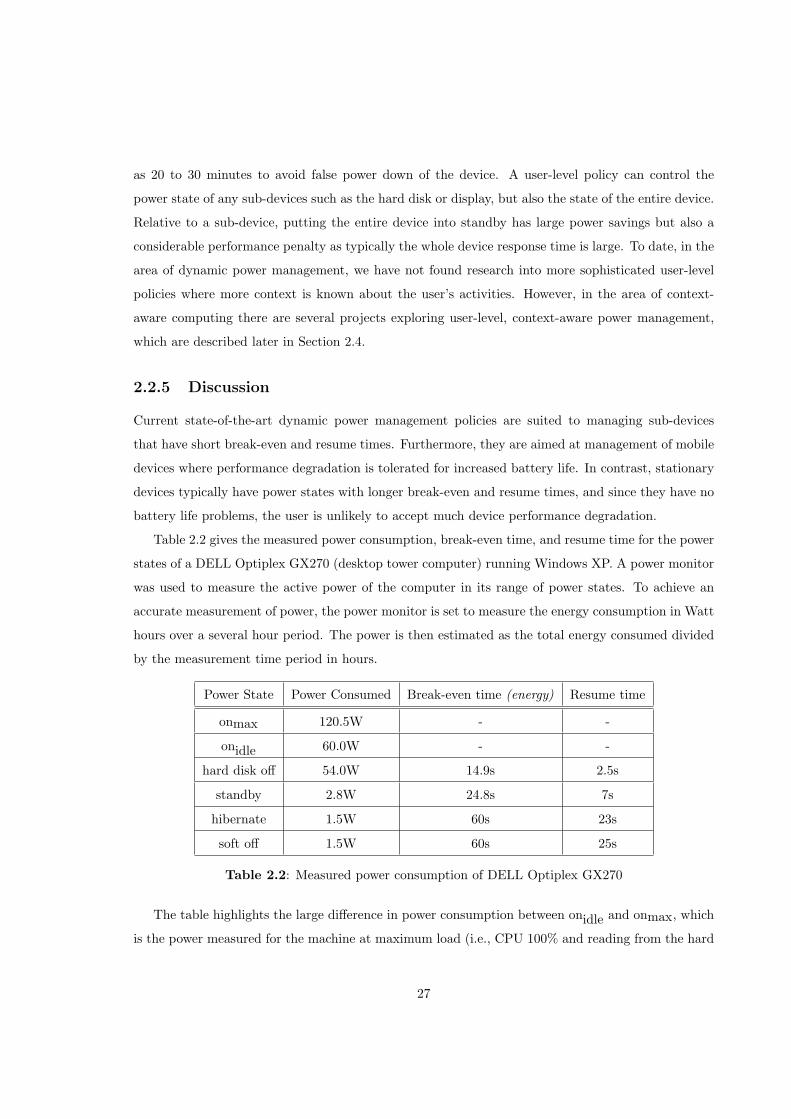
as 20 to 30 minutes to avoid false power down of the device. A user-level policy can control the
power state of any sub-devices such as the hard disk or display, but also the state of the entire device.
Relative to a sub-device, putting the entire device into standby has large power savings but also a
considerable performance penalty as typically the whole device response time is large. To date, in the
area of dynamic power management, we have not found research into more sophisticated user-level
policies where more context is known about the user’s activities. However, in the area of context-
aware computing there are several projects exploring user-level, context-aware power management,
which are described later in Section 2.4.
2.2.5 Discussion
Current state-of-the-art dynamic power management policies are suited to managing sub-devices
that have short break-even and resume times. Furthermore, they are aimed at management of mobile
devices where performance degradation is tolerated for increased battery life. In contrast, stationary
devices typically have power states with longer break-even and resume times, and since they have no
battery life problems, the user is unlikely to accept much device performance degradation.
Table 2.2 gives the measured power consumption, break-even time, and resume time for the power
states of a DELL Optiplex GX270 (desktop tower computer) running Windows XP. A power monitor
was used to measure the active power of the computer in its range of power states. To achieve an
accurate measurement of power, the power monitor is set to measure the energy consumption in Watt
hours over a several hour period. The power is then estimated as the total energy consumed divided
by the measurement time period in hours.
Power State Power Consumed Break-even time (energy) Resume time
onmax 120.5W - -
onidle 60.0W - -
hard disk off 54.0W 14.9s 2.5s
standby 2.8W 24.8s 7s
hibernate 1.5W 60s 23s
soft off 1.5W 60s 25s
Table 2.2: Measured power consumption of DELL Optiplex GX270
The table highlights the large difference in power consumption between onidle and onmax, which
is the power measured for the machine at maximum load (i.e., CPU 100% and reading from the hard
27

disk). The hard disk off state is just onidle with the hard disk powered down, whereas standby powers
off all sub-devices except the random access memory (RAM) and the network card. The state of the
system is stored in RAM so it can be resumed in a reasonable amount of time (˜7 seconds). Hibernate
is a slightly lower power state where the state is saved to hard disk and soft off is the state where the
PC is physically shut down, no system state is saved, but it is still connected to the mains. Both of
these states have very long resume times as the operating system needs to be rebooted, making them
impractical for dynamic power management.
Typically, a desktop computer will spend most of its operating time in the onidle state. Switching
the hard disk off gives a modest saving of 6W (10% of the base onidle consumption), whereas switching
the PC to standby gives a very significant saving of 57.2W (95% of the base onidle consumption).
Modern PCs are designed to achieve these very low power standby states by use of dual mode power
supplies, which provide trickle power when the PC is in standby, enough to power the network card
and refresh the RAM [34]. Making this state change to system standby has significant savings over
putting individual components into standby but also significant performance penalties. The system
standby state has a significantly longer resume time than the hard disk. Furthermore, putting the
system into standby affects the visible state of the system as the display will also be powered off.
As an example, using a threshold policy with Tidle of 10 seconds at the user-level to power the
system to standby is clearly unrealistic. It would cause unworkable performance degradation through
frequent false power downs and manual power ups. This being due to an inability to predict relatively
long idle periods and an inability to predict when next to power up the device. Thus, the limitations
of current dynamic policies for management of stationary devices are:
1. They are not capable of accurately and quickly predicting when the user will not be using the
device for a relatively long period of time (e.g., 1 minute, 5 minutes, 10 minutes).
2. They always incur some degree of performance degradation as they cannot predict when the
next user request may arrive.
To achieve the large savings of system standby and not incur large performance penalties we must
develop policies that can (a) accurately and quickly predict long idle periods (order of minutes)
and (b) predict when the user will make the next request. The first requirement brings us close to
the oracle policy in terms of power efficiency and the second requirement enables us to minimise
performance degradation. We believe that users of stationary devices will not tolerate significant
performance degradation as energy is not critical. Also, we believe a realistic solution will require a
relatively low cost of implementation. Finding a power management solution that is transparent to
28

the user with little additional overhead is key.
2.3 Context-aware computing
Dey [17] gives one of the most cited definitions for context and context-aware computing.
“Context is any information that can be used to characterise the situation of an entity. An
entity is a person, place, or object that is considered relevant to the interaction between
a user and an application, including the user and application themselves.”
The definition is user-centered, focusing on users’ interactions with computing devices. In particular,
it envisions the main applications being for mobile devices where the users’ and applications’ context
may change often. While context can be used for power management of mobile devices, this research
only explores its application to stationary devices. Dey’s definition of context is still relevant to the
application of power management for stationary devices as a user’s context will change often with
respect to the stationary devices in the environment. Dey goes on to define the primary types of
context to be location, identity, activity and time2, and gives a general definition for a context-aware
system.
“A system is context-aware if it uses context to provide relevant information and/or ser-
vices to the user, where relevancy depends on the user’s task.”
An example model for context-aware computing suited to CAPM is detailed next.
2.3.1 Context-aware computing model
Biegel et al. [4] describe a context-aware computing middleware, based on the sentient object model,
to ease the development of context-aware applications. They state that the pervasive computing
function should necessarily be autonomous and proactive and give a definition of context that is less
centered in user interaction.
“Context is environmental information that an application may use to autonomously and
proactively fulfill its goals.”
At the core of the model is the sentient object abstraction (see Figure 2.9). The model uses an
event-based programming paradigm for communication between sentient objects. The solid arrows2This can also be defined as the where, who, when and what (i.e., what is the user doing).
29

Consume Produce
Datacapture &
fusionContext
hierarchyInference
engine
Sensor
Actuator
Sentient object
Software event
Real-world event
Figure 2.9: Sentient object model
show software events and the dashed arrows show physical events. The sentient object consumes
events from either physical sensors or other sentient objects, and produces events that are either
consumed by other sentient objects or actuators for control of the physical environment. A sentient
object provides support for data capture and fusion, a context hierarchy and an inference engine for
intelligent processing of sensor events.
The data capture and fusion component uses a filtering mechanism so that only relevant events
are passed to the sentient object and the fusion mechanism is based on an inference technique called
Bayesian networks, which uses probability to derive high-level contexts from noisy, low-level, multi-
modal sensor data. The context hierarchy is structured into three layers. The top-level mission
context defines inputs that are of interest to the sentient object and rules that are always valid;
several major contexts define distinct strategic objectives of the sentient object and, finally, sub-
contexts define operational actions carried out in fulfillment of a major context. The inference engine
uses a production rule-based system which fires actions when the object is in a particular context.
The rules provide a natural approach to representing knowledge within the system and the context
information derived from the sensor inputs is stored as facts in the rule engine.
The CAPM framework is loosely based on this sentient object model. For this thesis, the frame-
work implementation has focused on the core components of data capture, fusion and inference. To
enable more distributed operation it could be plugged into the sentient object middleware with each
30

power manager being implemented as a sentient object.
2.3.2 Properties of sensors and multi-sensory information
Gassmann et al. [25] state key properties of physical sensors are sensor accuracy, reliability and cost.
It is important to consider the accuracy of measurement required by an application. For example, is
location required to +/-5m or to +/-5cm. Secondly, the reliability of the sensor is important, i.e.,
how long will it last without maintenance and/or replacement. Finally, for practical applications, the
financial cost of the sensor needs to be considered.
The raw data from the physical sensors are combined/fused to provide multi-sensory information.
Luo [40] states that there are four fundamental properties of multi-sensory information: redundancy,
complementarity, timeliness and cost. Redundancy occurs when multiple sensors perceive the same
feature in the environment, which can reduce the overall uncertainty of the information. Complemen-
tary information from multiple sensors allows features in the environment to be perceived that are
impossible to perceive using just the information from each individual sensor operating separately.
Information may be more timely using multiple sensors by parallelising the information processing.
Information from multiple cheaper sensors may be less costly than using one more expensive sensor
to provide the same quality of information. For his analysis Luo defines cost in purely financial terms.
Other costs can be consumption of computing resources (e.g., CPU cycles) and consequently energy
consumption. Multiple cheap sensors might be less expensive to purchase but a multi-sensor system
may consume more computing resources and more energy.
Luo draws a distinction between multi-sensor fusion and integration. Multi-sensor integration
refers to the complementary use of information provided by multiple sensors, whereas multi-sensor
fusion is the actual combination of different sources of sensor information into one representational
format. Redundant information is usually fused at a lower level of representation compared to com-
plementary information, which is usually either fused at a higher level or provided directly to different
parts of the system without being fused. The advantage of more redundancy is increased certainty,
of more complementarity is increased number of perceived features, and of increased timeliness is
increased ability to react in time to a particular situation.
2.3.3 Granularity versus cost
Intuitively, finer-grained context can be obtained by adding more, different types, and more accurate
types of sensor into a space. Observing additional features enables detection of more distinct pat-
terns/cues for finer-grained context. This more certain, more accurate, complementary, and timely
31

information enables applications to make better and more timely decisions. However, also intuitively,
the more sensors there are and the more feature processing, the more the resource and energy cost
of the information.
For example, coarse-grained location/presence information can be a good cue for a person about
to use their PC, if for example, their behaviour is that they always check their email when they
re-enter the office. For other users it may not be a good cue, they may often pop in and out of their
office without checking their email and without using the PC3. Adding additional sensors to the scene
may help us do better. For example, knowing the time of day could help in determining whether
they are about to use their PC (e.g., they always check their email first thing in the morning, after
lunch and at the end of the day). Time of day is cheap to obtain but does depend on the user being
very regular in their behaviour. How well this works depends on the user’s usage pattern. Adding
other physical sensors could improve the situation, for example, to detect whether the user is alone
or with others, where the user is in the space, or whether the user is moving towards the PC. These
observations could possibly be made with additional sensors such as acoustic, video, object ranging,
and more accurate location, to try to establish finer-grained context. Example user context, from
coarse to finer grained, could include present, not present, alone, with others, taking a
break, reading, writing, talking, on telephone, in meeting, sleeping, using computer,
not using computer. Some activities can be interleaved and also, there can be dependencies
between activities. For example, if reading was detected we could infer not using computer,
although we would still be uncertain for how long the person will remain reading and not using the
PC.
As the primary objective of CAPM is to minimise overall energy consumption, there is a bound
on the granularity of context that is appropriate. Overstepping this bound and the system will start
consuming more sensor energy than the device energy it is saving due to the additional context. The
additional complicating factor is that user-perceived device performance must also be added to the
cost equation. To date we have not found any work that explores this boundary, i.e., the balance
between granularity of context and its cost (energy and device performance) for context-aware power
management.
The following section reviews the current state-of-the-art context-aware power management ap-
plications. The applications are loosely ordered by their increasing use of sensors and sophistication
in the techniques used to determine finer-grained user context.3These users may check their email with a hand-held device.
32

2.4 Context-aware power management review
A few projects have explored context-aware power management. In the following sections we provide
an overview and analysis of these projects.
2.4.1 A context-aware approach to saving energy in wireless sensor net-
works
Chong et al. [11] present a framework for power management of sensors in a sensor network, the objec-
tive being to minimise the energy consumed by the sensors, which are battery powered4. They state
that current work in this area has focused on improving energy-efficiency of the hardware, tailoring
sensor designs to be efficient for specific applications, and improving the efficiency of communication
protocols. Their context-aware power management framework addresses power management at the
application level and is not application specific. The central idea is to use changes in the sensed
context to adapt the operating (power) states of the sensors, thereby saving energy when the sensors
are not being fully utilised by the particular application. An example they give is of a pig farm where
pig sties are monitored for temperature, light and sound. Detection of no (or minimal) sound for a
long period is a pattern in the data that relates to a context of pigs temporarily out of sty.
The application developer manually maps this context to a power management function that reduces
sensing frequency for the sensors in the sties. When the pigs come back the sensing frequency is
returned to normal.
The framework consists of three main components, context discovery, context trigger engine and
communication. These components correspond loosely to the sentient object model described in Sec-
tion 2.3.1. Context discovery is responsible for data capture and fusion of raw sensor data into context.
Currently this fusion of raw data is done by manually configured if-then rules. A future version will
use a data mining service to automatically discover new contexts (i.e., frequently occurring patterns
in the data). The context trigger engine maps sensed contexts to power management functions that
change the operating (power) states of the sensors. Again, these are manually configured rules, as in
the example above, if pigs temporarily out of sty then reduce sensing.
The evaluation of the framework is based on a twenty-minute simulation of the pig sty scenario.
They compare the energy consumption of their context-aware power managed network with a network
with no CAPM. The context-aware power manager modifies the sensing frequency of the sensor nodes
between 1-second, 10-second and 100-second sampling frequencies depending on what context the4This reduces the frequency of battery replacement.
33

application is in. They report an estimated power saving of 33% compared to the control experiment,
which keeps the sensing interval fixed at 1 second.
2.4.1.1 Analysis
To summarise, the sensors used were temperature, light and sound to infer when pigs were not
present in their stie. The inference technique was a simple if-then rule-based approach. The work is
currently at quite a formative stage with few real results for proper evaluation. Data would need to
be collected from a real pig sty to properly evaluate the actual usage patterns and subsequently the
actual potential savings. Furthermore, they do not evaluate what impact the power management may
have on the performance of the pig sty monitoring application. For example, when the pigs re-enter
the sty, what effect does the delay in resuming the frequency from 100 seconds to 1 second have on
the monitoring application. Is there a loss of valuable data? Another point to evaluate would be the
time required by the operator to manually code the mappings from contexts to power management
functions.
Finally, the scenario is a simplified study of CAPM as the power management is based solely on
occupancy, which is detected using a simple acoustic sensor. The logic reduces to, when the pigs leave
the sty, reduce the sensing and when they return increase it again. The simulated scenario does not
give any real insight into the issues of CAPM. However, the paper does show that there is interest in
the area of context-aware power management.
2.4.2 Location aware resource management in smart homes
The MavHome project’s goal is the creation of an intelligent home environment [16]. Roy [55] focuses
on resource (power) management of the electrical devices in a home environment based solely on user
location and predicted future location. The MavHome floor plan (see Figure 2.10) is divided into 15
zones containing 11 RFID5 readers and 9 pressure mats. Zone connectivity is represented as a simple
graph with each edge of the graph being annotated with a list of the sensors a user would pass to get
from one zone to the next. These are termed paths and there may be more than one path between
zones.
Zones and sensors are labelled alphabetically. The user’s symbolic location is determined by
sampling the 20 sensors and user mobility is captured as a string of characters, for example, ajlloojh-
haajlloojaajlloojaajlm, signifying the user passed from sensor a to j to l to l and so on. The sensors5Radio frequency identification.
34

RFID reader
pressure mat
mainbedroom dining
room
livingroom
bedroombedroom
garage
wa
sh
roo
m
kitchen
ba
thro
om
ba
thro
om
Figure 2.10: MavHome floor plan
give room-level location granularity with the use of pressure mats to divide up the large open plan
kitchen, dining, and living rooms. There are two parts to the CAPM algorithm:
1. When the user leaves a zone, predict the path to the next zone based on their current zone and
the user’s mobility history.
2. Switch on all devices along the path. (Presumably all devices in the previous zone are switched
off after a short timeout period.)
Emphasis is given to the user mobility prediction part of the algorithm. The Lempel-Ziv text com-
pression scheme is used to compress user mobility strings, which are subsequently sent to a server and
stored in a search trie. The compression technique finds regularly occurring patterns in the data and
also reduces the cost of data acquisition as the data strings are compressed. The mobility prediction
scheme makes its decisions based solely on the history of the room-level user mobility patterns and
does not take into account other valuable data such as the time of day or day of week to aid its
prediction.
2.4.2.1 Analysis
To summarise, the sensors used were RFID readers and pressure mats to obtain room-granularity
location. A compression technique was used to discover user mobility patterns, which drove the
power management policy of switching devices on before the user reached the predicted next zone.
The policy to switch on all devices in the user’s predicted path from one zone to the next is naive.
35

First, they do not categorise the devices into continuous and intermittent devices. Continuous devices
experience no idle periods during their operation and typically they are devices that carry out a well-
defined task such as making coffee, cooking food, washing clothes etc. Only intermittent devices (i.e.,
devices that experience idle periods) are suitable for context-aware power management. Intermittent
devices include lighting, sound, video display, heating, cooling and ventilation. Second, a user will
typically not require all intermittent devices all the time. Switching on all of these devices all of the
time will potentially frustrate the user and waste energy.
User-perceived performance of power management algorithms is sensitive to even small delays in
response and subtle changes from the normal operation of the device. Mozer cites even a 700ms
delay in his system as enough to annoy the user [43]. Since the predictive policy was not actually
implemented in reality it is hard to estimate what the real user-perceived performance of the policy is.
Our first concern, however, is the delay in actuation caused by the compression approach withholding
sensor data from the policy. They also assume negligible transfer time from sensor to policy and back
to actuator, which is not the case. Second, the path prediction success is 85% meaning 15% of the
time the predictive policy will switch on the wrong set of devices and the user will be left to manually
switch these off and the desired ones on. For the system to be workable we believe the predictive
success has to be close to 100% to avoid user annoyance.
Finally, there is no evaluation of potential energy saved nor energy consumed by the system.
Probably the most fundamental flaw in the system is assuming that the user will want all devices
in their future path switched on. There is no mechanism for capturing the user’s preferences or
behaviour. A possible improvement to the system is reviewed next.
2.4.3 Improving home automation by discovering regularly occurring de-
vice usage patterns
Also part of the MavHome project, Heierman [27] developed a data mining technique, termed episode
discovery (ED), to discover significant patterns in a user’s device interactions to improve home au-
tomation. ED could be applied to Roy’s location-aware power management policy above to improve
its effectiveness by discovering which devices are used at given times of the day. So, a device would
only be switched on when the user enters its vicinity and they regularly switch this device on at this
time of the day. He states the main challenge in discovering regularly occurring device usage patterns
is the excessive noise in the data. For example, it would not be desirable to automate appliance
interactions for random and frequent trips to the kitchen to get a drink of water.
Their data mining technique, ED, is influenced by several characteristics of device usage, (i) there
36

is no explicit start and end points to sequences of device interactions (episodes), (ii) the ordering of
interactions within the pattern must be discovered, (iii) the discovery needs to balance frequency with
pattern length, and (iv) the dataset is of moderate size allowing use of techniques not suitable for
large datasets. The technique mines the device activity stream to discover episodes that are closely
related in time. This enables the algorithm to discover events that occur on a daily basis and weekly
basis. An example they give is the sequence of devices the user switches on and off after they get out
of bed in the morning {alarm on, alarm off, bedroom light on, coffee maker on, bathroom light on,
bathroom video on, shower on}. An example weekly event occurrence is the water sprinkler being
turned on and off.
The ED algorithm uses a 15 minute sliding window to generate a complete set of candidate
significant patterns. This is achieved by incrementally processing the event stream. Each window
of events is a maximal candidate pattern. Within each maximal pattern there are the possible set
of “child” sub-patterns, which are pruned to prevent exponential explosion of the candidate set. ED
evaluates each of the candidate patterns using the minimum description length (MDL) principle. The
fundamental idea behind the MDL principle [54] is to view pattern learning (finding regularity in the
data) as compression. The more the data can be compressed the more we have learned about the data.
The MDL compression technique balances the length of patterns with their frequency, which Heierman
states is a good property for finding significant device interactions. The amount of compression
equates to the pattern’s significance and because a high level of confidence is required, a minimum
compression level of 80% was chosen to determine device interactions that are worth automating.
The algorithm is used to (i) improve a prediction algorithm’s accuracy by removing noise from its
training data and (ii) recognise regularly occurring device interactions that should be automated. The
algorithm is evaluated using synthetic data for two prediction algorithms, Incremental Probabilistic
Action Modelling (IPAM) and a Back Propagation Neural Network (BPNN). IPAM is a frequency
based prediction algorithm that maintains a probability distribution for the next event given the
current state. The synthetic data contains 5 randomly generated scenarios that cover typical device
interactions over a 6 month period. There were 14 regularly occurring daily and weekly patterns and
68 noisy patterns. The results (see Table 2.3) show that the ED algorithm significantly improves the
performance of the prediction algorithms for the synthetic data sets.
Table 2.3: Average Scenario Prediction Results [27]
IPAM IPAM+ED BPNN BPNN+ED
41.0% 73.6% 63.6% 85.6%
37

As a final analysis, they collected one month of real device interaction data from 6 participants in
the MavHome environment laboratory. The dataset consists of 618 device interactions contained in
it patterns which occur once a week, multiple times a week and randomly. From this data, ED was
able to correctly identify the patterns of three of the six inhabitants as significant episodes that occur
weekly, it was unable to discover the patterns that occurred multiple times in a week. Heierman
stated that further work was needed to discover the weekly patterns.
2.4.3.1 Analysis
This is an interesting paper as it demonstrates the discovery and use of device interaction patterns
over time. The sensors used are “device interaction” sensors (i.e., power on switches), time of day, and
the day of week. The ED algorithm uses a compression technique to discover the device interaction
patterns. The results show that the algorithm performs well for smoothing synthetic data to be used
by prediction algorithms (IPAM, BPNN). However, the discovery of significant device usage patterns
from real usage data is poor, only discovering weekly patterns for three of the six users (i.e., 50%).
This suggests that possibly there is not much regularity in users’ actual device usage or there is more
work to be done to improve the algorithms.
The technique could be added to Roy’s system with little additional energy cost and potentially
improve the performance. Unfortunately, there is no evaluation of this.
2.4.4 An adaptive fuzzy learning mechanism for intelligent agents in ubiq-
uitous computing environments
The iDorm project [10] has instrumented a real student dormitory for use as a test bed for pervasive
computing experiments. Doctor et al. [19] present a novel system for learning and adapting fuzzy
logic controllers to automate a user’s devices within the single-bed dormitory room. Their adaptive
on-line fuzzy inference system (AOFIS) uses an unsupervised, one-pass algorithm to extract fuzzy
membership functions and fuzzy rules from the data. The learned rules are applied to a fuzzy logic
controller that models the user’s behaviour. The rules map the sensor inputs to actuator outputs,
which in turn control the environment. Figure 2.11 shows the five phases of their architecture.
The system was run for a five-day period, monitoring the user for the first three days and then
automating the system for the final two days. The sensors used were internal light level, external light
level, internal temperature, external temperature, chair pressure, bed pressure and time measured on
an hourly scale. The actuators controlled four spot lights, a bed lamp, a desk lamp, a window blind,
the heater and two PC applications, a word processing program and a media playing program.
38

Useraction
Monitored change
Controller response
User
Capture data on userinteraction
Extract Fuzzy membershipfunctions from data.
Extract Fuzzy rules fromthe data.
Agent control and online creation/adaptation of Fuzzy rules.
Environment
Figure 2.11: Five phases of AOFIS [19]
In the initial monitoring phase the device usage data was captured. Whenever the user interacted
with a device a snapshot of the sensor readings and the actuator changes were recorded. This
generated a set of multi-input multi-output data pairs. In the next phase the data was categorised into
a set of fuzzy membership functions that map the raw sensor data into symbolic labels or predicates
(e.g., cold, warm, hot). These membership functions are extracted from the raw data using a statistical
clustering technique. An example membership function is ChairPressure{weight, noWeight}, which
categorises the chair pressure sensor readings into two categories weight and noWeight. Once the
membership functions are learned, they are fed to the fuzzy rule extraction phase.
The fuzzy rule extraction phase extracts multi-input multi-output rules to describe the rela-
tionship between the membership functions, and take the following form: if ChairPressure =
weight thenDeskLight = on6. Once the membership functions and set of rules are extracted from
the data, the fuzzy logic controller can start automating the device interactions on behalf of the user.
The agent is designed to continually learn new or modified rules, as the system may need to be tuned
and will need to adapt to the user’s behavioural changes. This is done by taking a snapshot of the
sensors, whenever the user makes a manual adjustment to the actuators.
Data captured in the three-day monitoring phase of the experiment was used to compare with
three other learning algorithms, genetic programming (GP), adaptive-neuro fuzzy inference system
(ANFIS), and a multi-layer perceptron neural network (MLP). The algorithms were trained on two
thirds of the data and tested on the other third. The AOFIS algorithm generated 155 rules from
the 272 training instances. Performance was based on the average scaled root mean squared error6This is our example to illustrate the author’s system.
39

in the algorithms’ predictions (i.e., the difference between what device interaction was predicted by
the algorithm and what device interaction actually happened). The results show that AOFIS (0.12)
performed marginally worse than the GP algorithm (0.11) and marginally better than the ANFIS
(0.14) and MLP (0.16) algorithms.
2.4.4.1 Analysis
To summarise, the sensors used were light, temperature, and pressure sensors to infer whether the
user was about to use a device (lighting, heating, media application). The technique they used
was a fuzzy logic controller, which includes learning and updating of its rules from past device usage
data.
The evaluation was only done for one user of the system, therefore it is not possible to tell if the
results are significant or not. The results show only marginal differences between the algorithms’
performance suggesting that there may not be any difference. Having more users do the experiment
would begin to indicate what variance exists in the system for different types of user. The on-
line performance was evaluated by running the fuzzy logic controller for a further two days. Its
performance was measured by monitoring the total number of rule adaptations over time. The
controller started with 186 rules from the 3 days and learnt another 120 rules in the subsequent two
days.
Figure 2.12: Rule modifications [19]
Figure 2.12 shows the number of rule modifications the system undertook over the two-day control
period. This equates to the number of times the user had to manually adjust a device because the
40

fuzzy logic controller failed to adjust it or adjust it correctly. The graph shows that on average there
was one modification every five minutes. One possible reason for this poor performance could be the
sparse number and type of sensors used (7 sensors in total) to control the 10 devices. The authors
explain the levelling off of adaptation on the afternoon of the second day as the system suddenly
performing better. This might also be explained by the user either having fallen asleep or having left
the room for this period.
Again, there is no evaluation of energy saved by the system and the results suggest the user-
perceived performance is poor, with many manual adjustments being required.
2.4.5 Lessons from an Adaptive House
The Adaptive House project [42] has a similar floor plan to the MavHome project but has a more
sophisticated CAPM framework that has been developed from eight years of actual implementation
and experimentation. The real-life experience from this project highlights the subtle requirements
for effective power management. Here user mobility prediction is only one component of the CAPM
framework and it utilises dozens of environment and user context variables in making the power man-
agement decisions. Also, the project focuses only on home comfort devices, namely air temperature,
water temperature and lighting devices. These devices fall into the category of intermittent use.
The system is composed of 75 sensors monitoring room temperature, ambient light, motion, sound
level, door and window positions, and outside weather and insolation. Actuators control a central
heating furnace, electric space heaters, water heating, lighting and ventilation. [43] concentrates on
the issue of lighting control, the objective being to automate the setting of lighting levels within the
house to maximise inhabitant comfort and minimise energy consumption. The main challenges are:
1. There are several lights in each room, each with 16 settings. The user prefers different lighting
moods depending on the task s/he is doing.
2. Motion sensors have a time lag in detecting user occupancy and there is delay in the X10
communications of 700ms causing a delay in system response.
3. Motion sensors do not detect the presence of a person very well. For example, a person could
be present in a room and reading but not moving.
4. The policy must satisfy two often opposing constraints, user comfort and energy consumption.
The lighting control system architecture, ACHE, is shown in Figure 2.13 below.
41

occupancymodel
anticipator
natural lightestimator
event-triggeringmechanism
stateestimator
costevaluator
Q-learningcontroller
lightswitches
sensors
lightdevices
Figure 2.13: Adaptive House Architecture (ACHE)[43]
It has two levels of abstraction that filter noisy sensors and provide higher-level information to the
Q-learning controller. This reinforcement learning technique models user discomfort and energy costs
and uses trial and error learning to minimise the total average cost. In classical decision theory, each
decision leads to a state s, which has a well defined reward R(s). There is a complete prior model of
the reward function, which can be used to learn an optimal policy. In reinforcement learning, there
is no prior knowledge of the reward function for each state and the algorithm attempts to learn an
optimal policy based on receiving infrequent reward signals. The ACHE Q-learning controller has a
partial model of the reward function. It can learn about other bad decisions in lighting level based
on the setting the user selects. If the decision was A and user corrected up to C, then any B lower
than A would also have been a bad decision.
The natural light estimator estimates natural daylight from raw sensors (as if the lighting was
turned off). The anticipator is a single-hidden-layer neural network that predicts if a zone will be
entered in the next 2 seconds. It runs every 250ms and its inputs are motion, door status, sound level,
zone occupancy and time of day. This component has been identified as not predicting sufficiently
accurately due to sparse sensor representation. This caused user annoyance when lights would go on
in an unoccupied zone. The occupancy model predicts whether a zone is occupied or not and the
inputs are motion sensed in zone, number of people in the house and motion in adjacent zones. The
state estimator forms a high-level state representation for decision-making with the most important
inputs being estimated user activity and natural light level. The user’s activity is estimated by zone
change frequency.
42

2.4.5.1 Analysis
The Q-learning policy costed energy ($0.072 per kWh) and user discomfort ($0.01 per manual ad-
justment, $0.01 per failed anticipation and $0.01 per false turn on) in dollar units and graphed these
costs over time. Figure 2.14 shows the energy cost per event dropped over time from 0.5 cent to 0.05
cent. However, it is not clear how this cost relates to the actual energy cost of the lighting.
Figure 2.14: Energy versus user discomfort [43]
The graph also shows the user discomfort cost starting at 0.1 cent per event rising to 0.8 and
decreasing again to 0.01 cent per event (after an error in the system code was fixed). These figures do
not really give a good idea of the actual user-perceived performance. The two main discomforts the
author experienced were the slow response of the system (due mainly to X10 communication delay)
and the occasional false anticipation of zone entry. This caused switching of lights on in unoccupied
zones. Surprisingly, there is no specific evaluation of the control of lighting level based on user activity
prediction. User activity is based only on recent user mobility patterns. For example, the user being
still for 5 minutes equating to the user reading and frequent zone change equating to cleaning
house. Mozer notes user activity classification as an interesting area for future research.
“ACHE, however, has no explicit representation of user activities, e.g., whether the inhab-
itants are preparing dinner, relaxing, studying, etc. Such an intermediate level represen-
tation could serve a valuable purpose, particularly in integrating sensor information over
time and increasing coherence of control decisions over time.”
Mozer states that the set of activities sufficient to characterise the typical behaviour of the inhabitants
is finite and could be inferred from sensor data. Being able to infer these activities could increase the
43

performance of the control decisions over time.
In summary, ACHE is the most advanced CAPM application that we know of, employing in total
75 sensors monitoring temperature, light, motion, sound, door and window positions, and weather to
infer not using and about to use of lighting devices. The techniques used are a neural network for
mobility prediction, and a reinforcement learning technique for the decision policy. However, there
is no evaluation of the potential energy savings of the system nor its energy cost. Adding further
“activity classification” context can potentially improve system performance but it will also add to
the energy cost.
The following section gives an overview and analysis of the current state of the art in user activity
monitoring. Some of these techniques could potentially be used to improve CAPM.
2.5 User activity monitoring review
This section presents an overview and analysis of several projects in user activity monitoring, which
highlights how finer-grained user activity may be obtained but also the significant potential energy
cost of obtaining this context. This provides clear evidence of the need to evaluate the balance
between energy saving and energy consumed by obtaining finer-grained context. For CAPM it is not
simply a solution to obtain more context to solve the power management problem.
2.5.1 Inferring Activities from Interactions with Objects
Philipose et al. [52] propose that the sequence of objects a person uses while performing an activity
robustly characterises the activity’s identity. Their Proact system is applied to the area of elder care
where it is necessary to monitor whether people with early-stage cognitive decline are performing their
activities of daily living (ADLs) and how well they are performing them. They state the key challenges
are that (i) users can perform ADLs in various ways, so models of activities and recognition software
must adapt to this variety, (ii) the underlying sensors must report the features required robustly
across varying environments (such as light levels, sound levels, and locations), and (iii) there are
a large number of ADLs (20-30 classes with 1000s of instances). They further state that a system
should model each activity with minimum human effort. A subset of example ADL classes that were
used in the experiment are listed in Table 2.4.
The Proact system consists of three components, RFID sensors to detect object interactions, a
probabilistic inference engine to infer activities given the sensor observations, and a model creator to
generate the probabilistic activity models. Objects of interest are tagged with postage stamp sized
44

Table 2.4: Activities of daily living [52]
ADL ADL
1 Personal appearance 8 Caring for clothes and linen
2 Oral hygiene 9 Preparing simple snack
3 Toileting 10 Preparing simple drink
4 Washing 11 Telephone use
5 Housework 12 Leisure activity
6 Use of appliance 13 Infant care
7 Heating control 14 Taking medication
RFID tags. The user must wear a glove, which has a small RFID reader attached, to sense when the
user touches a tagged object. The main advantages of this system are that it robustly reports data
at object-level granularity and it is modular allowing more tags to be added to objects if extra detail
is needed for a particular activity. They note that the RFID information could be augmented with
other sensor streams to fill in any information gaps, but for the experiment they just used RFID. The
reader samples the environment twice a second and broadcasts any detected objects to a wearable
iPaq that forwards this data wirelessly to a workstation running the inference engine. The glove’s
batteries last for two hours at this duty cycle.
Activities are modelled as linear sequences of activity stages. For example, making tea is a three-
stage activity of boiling water, steeping tea in water, and flavouring tea with lemon, sugar, or milk.
Each stage is annotated with the objects involved and the probability of their involvement. The
probability combines three sources of ambiguity: sensor error, model error and modelling generality
(an object is sufficient but not necessary). Each stage may optionally have a time to completion
modelled as a Gaussian probability distribution. The models are converted into dynamic Bayesian
networks (DBNs) where the sub-activity is the query variable and the set of objects seen and time
elapsed are observed variables. The network probabilistically estimates the sub-activities from the
sensor data. Activity models are generated from a pseudo English description of the activity similar
to that used in recipe books. Once the objects involved in the activity are specified, the involvement
probabilities are mined from the Internet using word counts via the Google API.
The experiment chose 14 ADLs for evaluation (see Table 2.4) and tested the system using 14
subjects performing the ADLs in the author’s instrumented house (108 objects were tagged within
a few hours). Each user spent on average 45 minutes in the house to perform the 14 ADLs. When
the user touched something they heard a beep to confirm it was recorded. Because the experiment
45

was not meant to test the efficacy of the glove, the users were asked to retouch the object if they
did not hear the beep. While performing the tasks the subjects wrote down on a sheet of paper
which task they were doing. After the experiments were completed the sensor data streams were fed
to the inference engine to predict the most probable ADL at any given time. This was compared
with the activity sequence the subjects previously wrote down. When Proact correctly claimed an
activity occurred it scored a True Positive (TP), an incorrect claim scored a False Positive (FP), and
no claim when the activity actually occurred scored a False Negative (FN). Proact correctly inferred
that an activity occurred 88% of the time and of the activity instances that actually happened, Proact
detected 73% correctly.
Issues included, (i) the RFID not performing well near water (e.g., washing hands), (ii) ADLs
with few observations such as adjusting the thermostat were not easily distinguishable from noise,
and (iii) overlapping activities with the same starting point were not possible to detect. For instance,
when Proact detects someone entering the bathroom, there are four possible activities that are equally
likely. If they then pick up their toothbrush, the system infers oral hygiene, however if they then
use the toilet the system misses this activity as there was no starting point of entering the bathroom.
They state that they need to reconsider their activity model to solve this issue. Another possible
improvement is to include unsupervised learning of model parameters, such as the duration of sub-
activities to improve model accuracy. In future work they want to integrate other sensors, particularly
location sensors. Where a person is located can be a good discriminator of performing a certain task.
They also want to integrate the time of day into their inference model as the time of day influences
the probability of performing a certain task. Key challenges include modelling overlapping activities,
multi person activities, and more complicated temporal models.
2.5.1.1 Analysis
To summarise, the sensors used are device-interaction sensors and the technique of dynamic Bayesian
networks is used to infer activity from the sensor data. This is interesting work that could in theory
be applied to an office environment. Possible objects that could be tagged are the telephone handle,
writing pen, and tea cups, which could be used to infer activities such as on telephone, writing,
taking a break. However, in an office environment there does not appear to be as many activities
that can be detected by object interaction as compared with the typical activities of a person in the
home. Furthermore, the practical barriers of needing to tag objects and getting users to wear RFID
readers makes the approach not viable for power management in an office environment.
46

2.5.2 Discovery and Segmentation of Activities in Video
Brand et al. [7] state that hidden Markov models (HMMs) are the standard technique employed
for visual event classification. They are used widely in spoken word and visual gesture recognition
but they fall down when applied to more complicated systems, as it becomes non-trivial to manually
construct and train the HMM. An example more complicated system is the classification of significant
user activities in a video stream for an office environment. They propose an unsupervised approach
whereby entropy minimisation of the HMM does away with the need for careful hand-crafting of the
model.
A HMM consists of a dataset X and a hidden-variable probabilistic model whose parameters and
structure are specified by the vector Θ. The normal method for training the model is that one guesses
the structure of Θ in advance and then re-estimates non-zero parameters to maximise the likelihood
P (X|Θ). This becomes very labour intensive for more complex models. They state that related
models such as dynamic Bayesian networks, also require careful hand-crafting. In entropic estimation
the size of Θ, its structure, and its parameter values are learned simultaneously in an unsupervised
manner. Minimising entropy is in practice similar to maximising the regularity of the data (i.e., its
compressibility). They state that their technique is similar to the MDL technique described in Section
2.4.3.
Their first example application is to learn a model of office activity. They state the main challenge
being that office activities have a range of time spans from just half a second to pick up a phone
to several hours for writing. The HMM represents the image as a set of ellipse parameters fitting
the single largest connected set of active pixels in the image. Active pixels are the pixels that move
in the scene, as distinct from the stationary background. A statistical model of the background is
acquired to separate the foreground active pixels from the background. The HMM was trained using
30 minutes of data acquired when the user was active in the office space. The unsupervised entropic
training yields a set of significant office activity states/patterns (see Figure 2.15) that occurred during
the 30 minutes of activity.
By comparing the learned states with the actual video frames, the states were manually labelled
as to what activity they represent. Once labelled, the HMM can annotate the video stream with
the current user activity. They have shown that by using entropy minimisation, the HMM can
learn observed activity into highly interpretable hidden states. The discovered hidden states are not
guaranteed to coincide with events that are of interest, but they state in their experience they have
always been interpretable and useful. The example application they give is of detecting anomalous
behaviour in the office, such as the user sleeping in their chair and the office being occupied by a
47

Figure 2.15: Several learned states in the trained HMM model. (a) entering room, (b) at
computer, (c) at white board, (d) sitting, (e) on telephone, (f) looking for a key, (g)
writing, and (h) swiveling right. [7]
worker with different habits.
2.5.2.1 Analysis
To summarise, the sensor used is a web camera positioned beside the user’s PC to infer user activities
in an office environment. They use an unsupervised entropy minimisation technique to learn the
set of distinct user activity patterns and these activities are manually labelled after training. This
technique of using video to infer user activity gets over the practical problems of object tagging and
wearable readers from the previous technique. However, it is difficult to get a sense of how well the
unsupervised learning of activities works as they do not test the trained model against a hand labelled
video sequence. They only show that the technique does discover significant patterns in the video
and that these patterns are manually interpretable. In particular, activities (b) at computer and
(f) looking for a key look visually very similar, and also (d) sitting and (h) swivelling right
appear quite similar.
It would be interesting to apply this system to the problem of CAPM to see empirically how well
the technique works. The next section reviews a more advanced system including more sensors for
activity recognition and gives evidence for the concern of resource/energy consumption.
48

2.5.3 Layered Representations for Human Activity Recognition
Oliver et al. [48] present a layered hidden Makov model technique for performing sensing, learning
and inferencing at multiple levels of temporal granularity. They apply the model to a system named
SEER that infers user activity from real-time streams of video, acoustic, and computer interactions
in an office environment. They state that much of the previous work on leveraging video and acoustic
information to recognise human activities has centered on identification of a specific type of activity
in a particular scenario, for example, hand gesture recognition [12]. This work applies to recognising
more complex patterns of specific human behaviour, extending over longer periods in time.
They developed a formulation of layered hidden Markov models (LHMMs) and explored the
challenge of fusing the readings from binaural microphones, a USB web camera, and a keyboard and
mouse, to infer the activities, phone conversation (PC), face to face conversation (FFC),
ongoing presentation (P), distant conversation (DC), nobody in the office (NP), and
user present engaged in some other activity (O). They initially experimented with a single-
layered HMM, which generated a large parameter space, requiring large amounts of training data
and resulting in low classification accuracies. They state that standard HMMs suffer from a lack
of structure, an excess of parameters, and an associated over fitting of data when they are applied
to reasoning about long and complex temporal sequences with limited training data. Also, when
the system moved to a new office, copious retraining was typically necessary to adapt the model to
the specifics of the signals and user in the new setting. The layered formulation of LHMMs makes
it feasible to decouple different levels of analysis for training and inference. The system employs
a two-layer HMM architecture. The raw sensor signals are processed within a time window of 100
milliseconds to obtain feature vectors for the first layer of HMMs. Example features for the video are
motion density, face density, foreground density, and skin colour density. Example audio features are
the signal energy, the mean and variance of the fundamental frequency over a time window, and the
source location of sound. A history of the last 1, 5, and 60 seconds of mouse and keyboard activities
is also used. The first layer of HMMs classify these features with a time granularity of 1 second and
in the final stage, the second layer of HMMs represents the typical office activities associated with a
time granularity of 5 to 10 seconds.
They tested SEER in multiple offices and collected data from a range of users and environments.
The high-level layer is relatively robust to changes in environment. Only some of the lower-layer
HMMs needed to be retrained to tune their parameters to new conditions such as different ambient
noise, background images and illumination. The number of parameters to estimate is much lower
than the single-layered HMM implementation. Encoding prior knowledge about the problem in the
49

structure of the models decomposes the problem into a set of simpler sub-problems and reduces the
dimensionality of the overall model. They trained and tested the performance of the single-layered
HMM and LHMMs on 60 minutes of recorded office activity data (10 minutes per activity, 6 activities
and 3 users). They used 5 minutes of data for training and the other 5 minutes for testing. The
average accuracies on the testing data were 72.68% (standard deviation (STD) 8.15%) with the single-
layered HMM and 99.7% (STD 0.95%) with LHMMs. In summary, the accuracy of the LHMMs is
significantly higher than the single-layered HMM for the same amount of training data and LHMMs
are more robust to changes in environment requiring retraining of only the higher layer.
A further paper [49] presents an extension to SEER, S-SEER, which attempts to address the sig-
nificant CPU usage of the feature vector extraction algorithms. They say that, although the methods
have performed well, a great deal of video and acoustic feature processing has been required by the
system, consuming most of the resources available in a PC. They develop an approach, expected
value of information (EVI), which uses the principle of maximum expected utility to determine dy-
namically which features to extract from the sensors in different contexts. The EVI of computing
a feature combination fk (e.g., motion density and face density and audio energy) is the difference
between the expected utility of the system’s best action when observing the features in fk and not
observing them, minus the cost of sensing and computing such features. If the net expected value
is positive then it is worth computing the features. The additional computational overhead to carry
out the EVI analysis is O(M ∗ F ∗N2 ∗ J), where M is the maximum cardinality of the features, F
is the number of feature combinations, N is the maximum number of states in the HMMs, and J is
the number of HMMs.
They performed a comparative evaluation of the S-SEER system when executing the EVI selective
perception policy against two baseline policies, random selection and rate-based. Random selection
is a simple policy that selects the features at random on a frame by frame basis. Rate-based is a
heuristic policy that defines an observational frequency and duty cycle (i.e., period during which the
feature is computed) for each feature f . The observation frequency and duty cycle are determined
by processing a validation set of real-time data. In the experiment the selection policies select any
combination of the four possible sensors, vision, audio, keyboard and mouse activities and sound
localisation. The results are shown in Table 2.5.
The results show that the EVI algorithm performs very well across the set of activities, reducing
the accuracy only slightly and manages to reduce the average computational cost from 54.3% to
33.4%, out performing the baseline policies. Further observations they make from the experiment
are that at times, the system does not use any features at all when it is confident enough about
50

Table 2.5: Average accuracies and computational costs for S-SEER [49]
Recognition Accuracy
No policy EVI Rate-based Random
PC 100 100 29.7 78
FFC 100 100 86.9 90.2
P 100 97.8 100 91.2
O 100 100 100 96.7
NP 100 98.9 100 100
DC 100 100 100 100
Average 100 99.5 86.1 92.7
Computational cost (% CPU time)
No policy EVI Rate-based Random
PC 61.22 44.5 37.7 47.5
FFC 67.07 56.5 38.5 53.4
P 49.8 20.88 35.9 53.3
O 59 19.6 37.8 48.9
NP 44.33 35.7 39.4 41.9
DC 44.54 23.27 33.9 46.1
Average 54.3 33.4 37.2 48.5
the situation but also that the system guided by EVI tends to have longer switching time (i.e., to
realise when a new activity is taking place) than when using all the features all the time. In most
of the experiments the sound localisation was never turned on due to its high cost and relatively low
informational value.
Finally, in [50] they compare use of a HMM at the highest level to the use of a dynamic Bayesian
network for inferring high-level user activities. HMMs can be viewed as a specific case of the more
general class of dynamic Bayesian models. They state that DBNs present several advantages to the
problem of user modelling from multi-modal sensory information, DBNs can handle incomplete data
as well as uncertainty, they are trainable, they encode causality in a natural way, algorithms exist
for learning the structure of the networks and doing predictive inference, they offer a framework
for combining prior knowledge and data, and finally, they are modular and parallelisable. One
disadvantage they state is that they cannot handle continuous data very well.
51

Figure 2.16 shows the DBN model for inferring the user activity from the video, audio, sound
location (SL), and keyboard/mouse (KM) sensors. The experiments compare the accuracy of HMMs
versus DBNs and evaluate any practical advantages and disadvantages. They collected 90 minutes
of activity data (15 minutes per activity). Table 2.6 shows the recognition accuracy for HMMs and
DBNs with and without the selective perception.
SLT1
VideoT1
AudioT1
KMT1
ActivityT1
SLT0
VideoT0
AudioT0
KMT0
ActivityT0
Figure 2.16: S-SEER dynamic Bayesian network [50]
The results show that DBNs have better recognition accuracy for this problem and employing the
EVI selective perception policy incurs less loss of accuracy for the DBN. They state an important dif-
ference for selective perception is that the HMMs marginalise over the unobserved variables, whereas
with the DBN the previous time slice (T0) influences inference about the unobserved variables, im-
proving the accuracy.
2.5.3.1 Analysis
This is possibly the closest work to our research in the sense it uses similar sensors (video, audio,
keyboard/mouse) in a similar office environment. They appear to achieve very good results for
activity recognition but at a very high computational cost. Even with their EVI sensor selection
52

Table 2.6: Recognition accuracy [50]
HMMs DBNs
PC 97/98 95/90
FCC 99/97 97/97
P 86/88 99/99
O 93/100 99/99
NP 100/100 100/99
DC 91/70 96/96
Average 94.3/92.2 97.7/96.7
policy their activity recognition algorithm consumes 33.4% of CPU time (on average). From the
figures for desktop PC power consumption given in Section 2.2.5, this equates to an average power
consumption of 20.2 W which is 33.6% more than CPU idle consumption. This gives clear evidence
that there is a boundary of granularity for context-aware power management. Another concern with
S-SEER is the need for retraining of the lower layer of HMMs for different environmental conditions.
In practice it would be desirable for the system to require no initial training stage. It would however
be interesting to see S-SEER applied to CAPM to evaluate how well it performs in terms of energy
saving and user-perceived performance.
2.6 Summary
This chapter has introduced the two areas of dynamic power management and context-aware com-
puting and reviewed the current state of the art in dynamic power management and CAPM. The
field of user activity monitoring was also reviewed.
The review shows that current state-of-the-art dynamic power management policies are not suit-
able for power management of stationary devices. There is a need to develop policies that can (i)
accurately and quickly predict long idle periods (order of minutes), and (ii) predict when the user
will make the next request (order of seconds beforehand). To achieve this we need to obtain context
from the user of the device. In particular, about when the user is not using and when the user is
about to use a device.
Current state-of-the-art CAPM has focused on developing inference techniques for inferring such
high-level context from low-level, noisy, and incomplete sensor data. There has been some work in
the area of CAPM that points towards the need for finer-grained context to do better.
53

At the same time, there has been work done in the area of user activity monitoring for fine-grained
activity recognition. A range of techniques have been developed, including discovering patterns of
device interactions, video processing, and acoustic processing. There has been reasonable success with
recognition of user activities, the main challenges left being recognition of interleaved/overlapping
activities and the cost (CPU/energy consumption) of recognition.
This review has provided evidence that there is a bound to the granularity of context appropriate
for CAPM. In particular there is a need to explore the potential energy savings and energy costs
of such CAPM systems. To our knowledge there has been no research into what are the potential
savings of context-aware power management and what granularity of context is appropriate.
54

Chapter 3
CAPM Framework Design
In this chapter we identify the key requirements for CAPM and present the design of the CAPM
framework. At the core of the framework is a Bayesian network, which performs the context inference.
We justify the selection of Bayesian networks for context inference and go on to give a detailed
explanation of Bayesian networks and parameter learning of the networks. Finally, we show the
evolution of the Bayesian models that were developed for the CAPM framework. We begin the
chapter by presenting initial experimental results, which give an insight into the main issues that
need to be addressed by a CAPM system.
3.1 Initial experimental results
To explore the requirements of context-aware power management and gain insight into user behaviour
patterns, we first examined in detail the the use of location as a key piece of context for power
management of users’ stationary desktop PCs in an office environment. The objective was to minimise
overall electricity consumption of the system while maintaining acceptable desktop PC performance.
We were interested in the relation between the user’s location and their user behaviour (i.e., whether
they were using the device or not when in it’s vicinity). We implemented two simple location-aware
policies and performed 6 user trials, each over a period of a week. The trace data collected from
the trials was analysed to gain insight into the energy consumption and user-perceived performance
of the location-aware policies. The office spaces included personal and shared spaces, and there was
only one user per desktop PC. The two simple location-aware policies use the location context derived
from detecting users’ Bluetooth-enabled mobile phones. The policies execute on each desktop PC
and continuously poll to discover the presence of their owner’s Bluetooth phone in the area. The two
55

location-aware policies were:
1. Standby On Bluetooth (SOB). When the PC is on, the policy polls for the user’s phone via
the Bluetooth discovery mechanism. If the phone is not found the PC powers down to standby.
The user manually wakes up the PC when s/he next needs to use it.
2. Standby/Wake-up On Bluetooth (SWOB). When the PC powers down to standby the policy
passes control to a nearby server. When the server detects the phone again it sends a wake up
message to the user’s PC. (We used a server to implement wake up because as yet we do not
know of a Bluetooth device that can wake up the PC from standby).
Using the Windows power management API we recorded all power state change events for the PC
during each user trial. This included recording when the PC was powered down to system standby,
when it resumed to the on state, both automatically and manually, and when the PC was on but
idle for the last minute. The on-idle time enables us to estimate how much energy the policy wasted
by the machine being on but (potentially) not being used. Knowing the idle times enables us to
generate the oracle policy trace (see Section 2.1) and the range of threshold policy traces (see Section
2.2.1). The range of the Bluetooth connection was 10 metres and its latency was approximately 10
seconds (i.e., it could take up to 10 seconds for the Bluetooth inquiry to find the phone). We also
noted during implementation that sometimes the inquiry would not find the phone even though it was
there. To overcome this source of error it was necessary to duplicate the number of inquiries. This
polling process took approximately 90 seconds to complete so there was a significant delay before the
machine was powered down. Policy traces were collected from 6 separate user trials, 4 of which used
the SOB policy and 2 of which used the SWOB policy. Software was written for analysing the traces
in terms of energy consumption and user-perceived performance (i.e., number of manual resumes and
short standby periods). For each trace collected, the oracle policy trace and a range of threshold
policy traces were generated. For the SWOB traces, corresponding SOB policy traces were generated
by removing the automated resume events of the SWOB policy. We estimated the mobile phone
consumed an extra 6 Wh of energy over the 4-day trial due to extra recharging necessary because the
Bluetooth discover mode was on all the time. The extra energy consumed on the PC by the power
manager was not measurable and we considered it negligible. Also, for the SWOB policy we did not
take into account the energy consumed by the wake-up server, as we assume this functionality would
eventually be provided within the USB Bluetooth adapter. The 6 Wh has been added to the energy
cost of the location-aware policies.
56
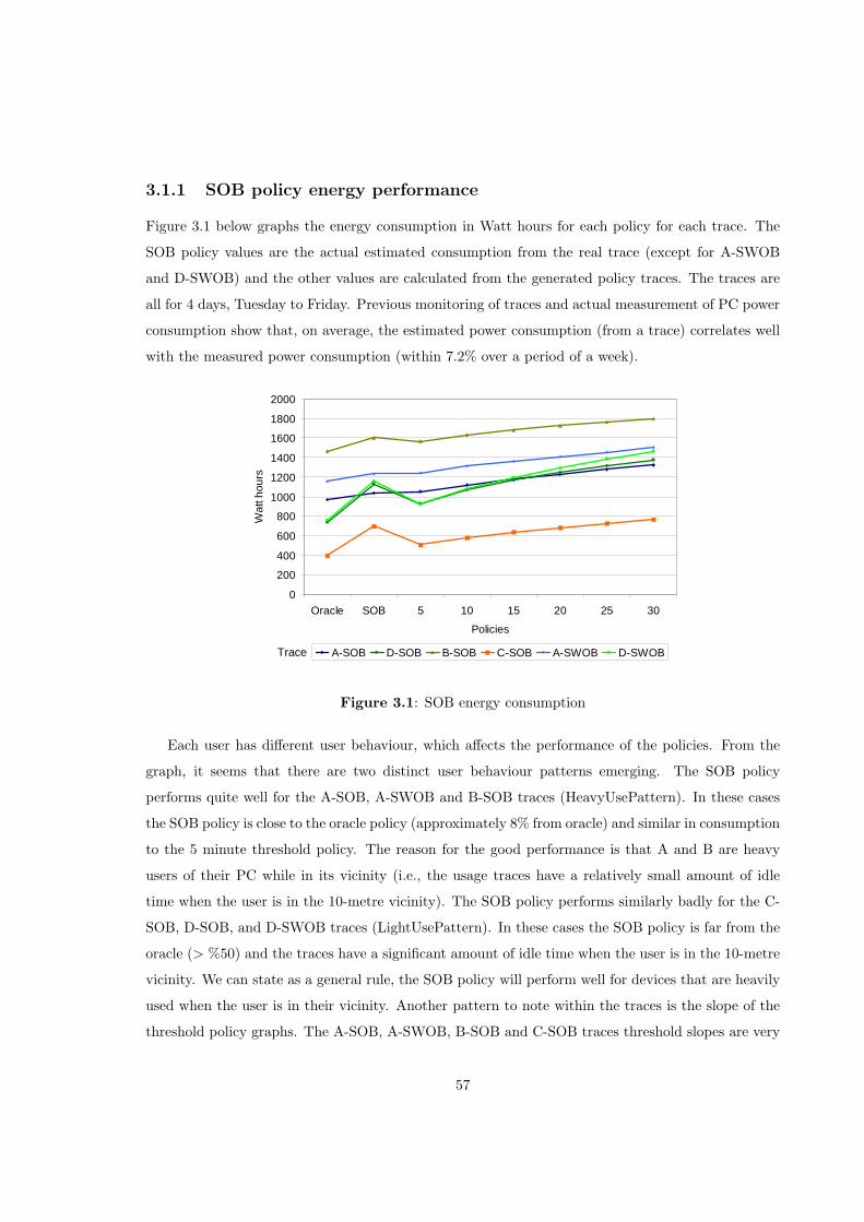
3.1.1 SOB policy energy performance
Figure 3.1 below graphs the energy consumption in Watt hours for each policy for each trace. The
SOB policy values are the actual estimated consumption from the real trace (except for A-SWOB
and D-SWOB) and the other values are calculated from the generated policy traces. The traces are
all for 4 days, Tuesday to Friday. Previous monitoring of traces and actual measurement of PC power
consumption show that, on average, the estimated power consumption (from a trace) correlates well
with the measured power consumption (within 7.2% over a period of a week).
Trace
0
200
400
600
800
1000
1200
1400
1600
1800
2000
Oracle SOB 5 10 15 20 25 30
Policies
Wat
t hou
rs
A-SOB D-SOB B-SOB C-SOB A-SWOB D-SWOB
Figure 3.1: SOB energy consumption
Each user has different user behaviour, which affects the performance of the policies. From the
graph, it seems that there are two distinct user behaviour patterns emerging. The SOB policy
performs quite well for the A-SOB, A-SWOB and B-SOB traces (HeavyUsePattern). In these cases
the SOB policy is close to the oracle policy (approximately 8% from oracle) and similar in consumption
to the 5 minute threshold policy. The reason for the good performance is that A and B are heavy
users of their PC while in its vicinity (i.e., the usage traces have a relatively small amount of idle
time when the user is in the 10-metre vicinity). The SOB policy performs similarly badly for the C-
SOB, D-SOB, and D-SWOB traces (LightUsePattern). In these cases the SOB policy is far from the
oracle (> %50) and the traces have a significant amount of idle time when the user is in the 10-metre
vicinity. We can state as a general rule, the SOB policy will perform well for devices that are heavily
used when the user is in their vicinity. Another pattern to note within the traces is the slope of the
threshold policy graphs. The A-SOB, A-SWOB, B-SOB and C-SOB traces threshold slopes are very
57

similar (10.8, 9.3, 10.3, 10.5) (LowFrequencyUsePattern) compared to the slope of the D-SOB and
D-SWOB threshold consumptions (18.0, 21.6) (HighFrequencyUsePattern). This indicates another
distinct user behaviour pattern in the traces that affects the performance of the threshold policies.
Intuitively, the higher the frequency of idle periods the worse the threshold policy performs from
oracle as it consumes extra power waiting to timeout, each time there is an idle period. So while
the SOB policy performs badly for all three LightUse user traces, due to the large number of idle
periods, the threshold policies perform worse for D-SOB and D-SWOB than C-SOB as user D has a
high frequency of idle periods (41 and 47 periods) compared to user C (24).
3.1.2 SOB policy user-perceived performance
We evaluated the quantitative user-perceived performance of the SOB policy by counting the max-
imum number of times (over the 4-day trace) that the user had to resume the PC in a 10-minute,
30-minute, one-hour, four-hour and eight-hour period. Figure 3.2 graphs the performance values per
user trace for the eight-hour period (The other periods have a similar pattern but with less resume
events). The Threshold-5 policy shows the HeavyUse traces having (7, 8, 9) resumes in an eight-hour
period compared to the LightUse traces (11, 12, 14). As would be expected the performance improves
as the threshold increases, with 20 minutes appearing to reach saturation (i.e., after this threshold
there is little improvement in performance). What is interesting to note is that for the HeavyUse
traces, the SOB policy performs similarly to the Threshold-5 policy but for the LightUse traces, the
SOB performs considerably better (7, 7, 7 resumes compared to 11, 12, 14). This intuitively makes
sense, as the HeavyUse users do not allow the Threshold-5 policy to power down while in the of-
fice, whereas the LightUse users would. So, another general rule is that the SOB policy keeps the
user-perceived performance acceptable for LightUse users.
A qualitative survey of the users revealed that for 2 of the users the performance penalty of
resuming the PC every time they came back to their office would not stop them implementing the
SOB policy. The other 2 users thought it necessary that the PC would resume automatically to avoid
the performance penalty. Clearly user-perceived performance is subjective and there is a balance for
each user of how long the standby period should be to justify the subsequent performance penalty
(i.e., a performance break-even time). Figure 3.3 shows the standby period frequency in minutes for
the SOB and Threshold-5 policies for the D-SOB (LightUse) trace. The graph shows the Threshold-5
policy has many more short standby periods. Also, the total number of standbys for the SOB policy
is 24 compared to 52 for the Threshold-5 policy. Therefore, 28 of the Threshold-5 policy standbys
occurred when the user was in the vicinity. Clearly, these short standby periods when the user is in
58

0
2
4
6
8
10
12
14
16
SOB 5 10 15 20 25 30
Policies
No.
of r
esum
es
A-SOB 8 D-SOB 8 B-SOB 8 C-SOB 8 A-SWOB 8 D-SWOB 8Trace
Figure 3.2: SOB user performance
the vicinity would severely degrade the user-perceived performance, making the Threshold-5 policy
unlikely to be implemented by any user.
0
2
4
6
8
10
12
14
16
18
20
1 3 5 7 9 11 13 15 17 19 21 23 25 27 29 31
Standby period (minutes)
No.
sta
ndby
s
SOB Threshold 5Trace
Figure 3.3: Standby period frequency
3.1.3 SWOB policy energy performance
The SWOB policy is an extension to the SOB policy where the PC powers up again when the mobile
phone is next detected in the 10-metre vicinity. For this reason we chose to evaluate the policy
59

with just two user trials. Figure 3.4 shows the policies’ energy consumptions for the A-SWOB and
D-SWOB traces. The graph compares the SWOB policy to the generated oracle, SOB and threshold
policy traces. Again, the two users have similar performance to their original traces with A-SWOB
performing well and D-SWOB performing badly compared to the oracle. Also, again the slope of the
threshold performances is similar to the original user traces. For A-SWOB the SWOB policy energy
performance is very similar to the SOB policy but for D-SWOB it is significantly worse. The increase
in energy consumption is caused by the SWOB policy automatically resuming the PC when the user
enters the vicinity. Hence, the PC can be on and idle before the user requests its use. The trace
distinguishes between when the PC is resumed automatically (i.e., over the network) and when the
user first pressed the keyboard after being in standby. So, we can measure the time from when the PC
is resumed automatically until when the user first uses the PC. We call this period the auto-on-idle
period. There are significantly more auto-on-idle periods for the D-SWOB trace (154 minutes in
total) than the A-SWOB trace (5 minutes in total). Also, there were 14 occurrences in the D-SWOB
trace where the PC was resumed and later went back to standby without being used by the user. In
interview after the experiment, user D stated that he would nearly always use the PC immediately
after entering the room. If this is true, it suggests that the PC was automatically resumed when the
user passed by the room.
0
200
400
600
800
1000
1200
1400
1600
Oracle SOB SWOB 5 10 15 20 25 30
Policies
Wat
t hou
rs
D-SWOB A-SWOBTrace
Figure 3.4: SWOB energy consumption
60

3.1.4 SWOB user-perceived performance
On average the Bluetooth discovery took approximately 10 seconds to discover the mobile phone and
the desktop PC takes approximately 7 seconds to fully resume from standby. Therefore, under the
SWOB policy it took approximately 17 seconds from the time the user enters the 10-metre vicinity
until the PC resumes fully, ready for use. To evaluate the user-perceived performance of the SWOB
policy we have to determine whether the PC was resumed in time for the user. Figure 3.5 shows the
graph of auto-on-idle period frequency in seconds for both traces.
0
5
10
15
20
25
30
1 4 7 10 13 16 19 22 25 28 31 34 37 40 43 46 49 52 55 58 61
Auto-on period (seconds)
No.
aut
o-on
per
iods
D-SWOB A-SWOBTrace
Figure 3.5: Auto-on-idle period frequency in seconds
The graph shows the D-SWOB trace to have few short periods (3 periods < 8 seconds) compared
to the number of longer periods (25 periods > 60 seconds). On the other hand the A-SWOB trace has
relatively many short idle periods (10 periods < 8 seconds) compared to number of periods greater
than 60 seconds. The auto-on-idle period is measured from when the PC starts to resume and it takes
approximately 7 seconds before it resumes fully and can be used. Therefore the data suggests that user
A experienced 10 delays in waiting for the PC to fully resume and user D experienced 3 delays. The
length of the delay is partly dependent on the geographical layout of the user’s return path and how
long it takes the user to return to their PC after they have entered the 10-metre vicinity. In general,
the current Bluetooth discovery time makes the auto wake up of the PC borderline functional and
very dependent on the user’s return path and their time to reach the PC. A more responsive sensor
could improve the SWOB policy’s user-perceived performance and be less dependent on geographical
layout.
61

3.1.5 Conclusions
The experimental user trials and subsequent policy trace analysis has highlighted several user be-
haviour patterns that affect the performance of the power management policies. The location aware
SOB and SWOB policies perform well energy-wise for HeavyUse users where the device is used a lot
when the user is in the 10-metre Bluetooth vicinity. For LightUse users they begin to deteriorate,
consuming energy when the user is in the vicinity but not using the device. For FrequentUse users
(i.e., the user uses the device many times during the day) the threshold policies deteriorate as energy
is wasted every time the policy waits for the timeout period. The SOB and SWOB policies are less
affected by this FrequentUse pattern, as the timeout period is less (90 seconds).
The user-perceived performance of the SOB policy appears to be acceptable to some users but
not others. The performance remains constant for both HeavyUse and LightUse users while the
Threshold-5 policy performance deteriorates significantly for LightUse users. The SWOB policy user-
perceived performance is dependent on the geographical layout of the users return path and how long
it takes for the user to return to their PC after entering the 10-metre Bluetooth vicinity. This makes
it suitable for only some cases. Furthermore, the SWOB policy comes at a price in increased energy
consumption, particularly in the case of LightUse users and unsuitable geographical layouts (e.g.,
where the user passes by the office within the 10-metre range).
A further concern of implementing these policies is that of device lifetime. For many devices,
switching them on and off affects their expected lifetime. We have estimated the break-even due to
lifetime for a desktop PC to be around 2 minutes. The estimate assumes that the hard disk is the
first component to fail in the PC and is based on the lifetime figures for a given Sea Gate 80Gb
Barracuda ATA V hard disk and a typical usage trace taken from the experiment. The reliable
lifetime is estimated to be 600,000 power-on hours and 50,000 start-stop cycles. The lifetime of the
disk is fixed at 10 years and we assume 250 working days in each year. For the given usage trace and
lifetime of 10 years, the number of the number of allowable start-stop cycles per day is 19 and the
power-on hours is 4. The next smallest idle period in the trace is 2 minutes, hence it is not worth
powering down for this 2 minute period. Other devices have longer lifetime break-even times such as
fluorescent lighting (5 to 10 minutes)[63]. Figure 3.6 shows the total number of standby periods for
all traces, of which there are a significant number of short standby periods occurring. Policies may
have to take device lifetime into consideration when making their power off decisions.
62

0
10
20
30
40
50
60
70
80
90
1 3 5 7 9 11 13 15 17 19 21 23 25 27 29 31
Standby period (minutes)
No.
sta
ndby
s
A-SOB D-SOB B-SOB C-SOB A-SWOB D-SWOBTrace
Figure 3.6: Standby period frequencies (minutes)
3.2 CAPM requirements
From the experimental trials we have identified several requirements for CAPM.
• R1: Required context - CAPM requires the prediction of the context not using for at least
the given break-even period and about to use at least the resume time beforehand.
• R2: Context granularity - The most important result from the initial experiments is that
coarse-grained location alone is not sufficient to determine the detailed user behaviour necessary
for effective CAPM. Finer-grained context is needed to predict (i) the user in the vicinity but
not using the device and (ii) the user in the vicinity and about to use the device. Passing
by the device but not about to use it is a special case of scenario (i). The second scenario is
difficult to achieve, as one key advantage of coarse-grained location is that it is a distant sensing
device, i.e., it senses the user at a distance thereby enabling time for the device to resume before
the user requests its use. Saving energy by switching off devices in the near vicinity of the user
is difficult to achieve transparently.
• R3: Distant prediction - The second result is that there is a need for distant (time wise)
prediction to offset delay in sensor response and long device resume times. For example, some
form of mobility prediction might overcome the problem of the latent Bluetooth sensing.
• R4: Distributed sensing - The third result is that there is a need for distributed sensing
of users and possibly recognition of user plans to predict longer future idle periods (for cases
63

where the device break-even time is an order of minutes). For example, given the results it
would not be sensible to switch off fluorescent lighting every time the user leaves the room as
this would cause premature failure. We define distributed sensing as the ability for sensor data
to be communicated amongst distributed sensing devices. For example, a sensing node in the
office bathroom could communicate the user’s presence with the power manager of the user’s
desktop PC in the office.
• R5: Decision under uncertainty - The initial experimental location-aware polices used
a simple rule-based design where, observed sensor states are matched to power management
actions. There is no representation of uncertainty, which is required in most real-world decision
applications to account for incomplete and noisy data [35]. Given a level of certainty in whether
the user is not using or about to use the device, a decision can be made as to which power
management action to take.
• R6: Adaptation - The simple rule-based design has no learning of new rules based on usage.
This design would not scale well to accommodate more sensors, as the rules would become
increasingly complex making it successively harder to configure for each individual user. Some
form of learning technique is needed, which can continually learn from device usage history and
adapt to the user.
The CAPM framework addresses these requirements and its design is detailed next.
3.3 CAPM framework design
The design of the CAPM framework is loosely based on the sentient object model (see Section 2.3.1).
A sentient object encapsulates the CAPM power manager for a device. Each power manager can
execute a number of policies, one power-down policy for each device state and one power-up policy
for when the device is in a reduced power state. Communication is event-based, enabling sensing of
distant sensors (fulfilling R3 and R4). Filtering of sensors enables the power manager to consider
only information relevant to it. In our implementation, filtering is configured manually but some
“intelligent” mechanism could automate the selection of sensors most relevant to the device’s power
manager. Sensors can include any physical sensing devices, power state changes of other devices,
and “software sensors”, such as time of day, or day of week. The power manager controls the power-
down and power-up of the device through the device’s power management API. Currently power
management of computing devices is non-standard with each operating system having their own
64

API1. Development of a standard API would be advantageous for power management of heterogeneous
devices. Until this is achieved wrappers are needed for the various operating system APIs.
ConsumePowermanagementAPI
Datacapture &
featureextraction
Contextinference
Decisionmaking
Figure 3.7: CAPM framework
At the centre of the framework are the data capture and feature extraction, context inference, and
decision components. Our research has concentrated on the development, realisation, and evaluation
of these core components.
3.3.1 Data capture and feature extraction
This is the first layer of data processing. Raw sensor events are captured and in most cases prepro-
cessed to obtain relevant features. For example, a video signal could be captured and preprocessed
to obtain features such as density of foreground pixels, density of motion, density of face pixels, and
density of skin colour [48]. A Bluetooth detection event could be preprocessed using a counter to
count the number of times a Bluetooth tag has not been detected. This gives a history of when the
tag was last seen, for example, a count of 10 means the tag has not been detected in the last ten
polls. A value of 0 means the tag was detected in the previous poll. It is also possible that for some
sensors, their data can be passed onto the next layer unprocessed. For example, the prediction from
a mobility prediction service that a user is going to enter the room in the next 10 seconds.
Sensor events received via event messaging are more likely to be already preprocessed (to reduce
bandwidth), whereas events from sensors that are directly connected to the sentient object are more
likely to require preprocessing (feature extraction), e.g., a video signal from a web cam or an audio
signal from a microphone. The output from data capture and feature extraction is made available to
the context inference layer.1The ACPI standard currently only defines interfaces between hardware devices and the operating system, not
applications and operating system.
65

3.3.2 Context inference
The context inference layer is responsible for inferring more certain, higher-level context from the
low-level sensor and feature data (inference can also be termed sensor fusion). The inference can
involve combining redundant data to achieve more certainty and multi-modal data to infer context
based on a combination of the multiple sensor modes. This is the most challenging part of the data
processing as it is trying to infer high-level notions from low-level, noisy, and incomplete sensor data
and/or their features. In the framework, probability theory is used to deal with this uncertainty in
the data (fulfillment R5). This gives a level of confidence in the proposition of a certain context being
true. This probabilistic inference of the contexts not using and about to use is carried out using
Bayesian networks (fulfillment of R1). This context is made available for use by the decision layer.
The Bayesian network is trained based on observation of the user using and not using the device
(fulfillment of R6).
3.3.3 Decision
The decision layer is responsible for taking the power-management actions. The possible actions
depend on the current state of the device. When the device is on the possible actions are either to
remain on or to power down to a lower-power state. When the device is in a lower-power state the
possible actions are either to remain in the lower-power state or to power up the device. For the
initial version of the CAPM framework the decision layer was designed as a simple threshold rule. If
the probability of not using exceeded the given threshold (80%) then the action to power down was
taken. Likewise, if the probability of about to use exceeded the given threshold (60%) the action
to power up was taken.
The design could be extended by the use of utility theory. Utility theory estimates the expected
utility of an action based on the level of certainty it has in the state of the world, the potential benefit
of the action and the potential cost. Given these inputs, the decision is then simply a matter of
choosing the action with the highest expected utility. Expected utilities can be implemented using
decision nodes, which are an extension to standard Bayesian networks. This extended Bayesian
network is called a Decision network.
3.4 Selection of inference technique
We have identified that the key challenge for CAPM is inferring the user’s context correctly, which
is carried out by the context inference component. The job of this component is to infer from low-
66

level data the contexts not using and about to use given uncertainty in the data, i.e., noisy and
incomplete sensor data. Korb et al. [35] state there are at least three distinct forms of uncertainty:
1. Ignorance. This refers to either a lack of information or a lack of understanding of how the
system fully operates. Ignorance relates to the incompleteness of sensor data. It may not be
practical to observe every possible event in the event space.
2. Physical randomness or indeterminism. Even if everything was known about the system, there
would still be some degree of randomness or indeterminism in the sensors that would cause
uncertainty. Indeterminism relates to noisy sensor data. Sometimes sensors report erroneous
values through either faulty hardware or indeterminate protocols. For example, the Bluetooth
discovery protocol’s frequency hopping sequence may fail to discover a device that is actually
in the vicinity.
3. Vagueness. Assertions are sometimes not clearly defined or vague. For example, it is often
unclear whether to classify a human as brave or not, or a dog as a spaniel or not. For CAPM,
it can be unclear as to when a person is not using a device. For example, some people might
like the television on in the dining area when they are preparing food in the kitchen and some
people might like their PC display on when they are reading at their desk, in case an email
comes in. The notion of not using is subjective to the individual.
We now briefly highlight some of the inference techniques employed by the state of the art in context-
aware computing and provide a justification for our use of Bayesian networks. A Bayesian network is
a graphical model that represents causal relationships between entities and models the uncertainty in
the state of a system. The technique is based on probability theory, which provides the foundation for
reasoning under uncertainty. The specification of dependencies between variables leads to an efficient,
tractable method for calculating the probabilities.
Chong et al. (see Section 2.4.1) use a rule-based approach to inference in the implementation of
their sensor fusion component. Russell and Norvig [56] give a good overview of rule-based inference
and the reasons why it is no longer used. They state that rule-based inference systems have three
desirable properties:
1. Locality. Given a rule of the form A ⇒ B (fact A implies proposition B), then B can be
concluded given fact A. It is not necessary to consider any other rules.
2. Detachment. Once a logical proof is found for a proposition B, the proposition can be used
regardless of how it was derived.
67

3. Truth-functionality. In logic, the truth of complex sentences can be computed from the truth
of the components.
There were several attempts to represent uncertainty in a rule-based inference system that retained
these desirable properties. The central idea was to attach degrees of belief (probability) to propositions
and rules and to devise purely local schemes for combining and propagating those degrees of belief.
The belief in the rule is assumed constant and specified by the knowledge engineer. For example,
A 7→0.9 B is read as fact A implies B with 90% probability. However, [56] states that the properties
of locality, detachment and truth-functionality are not appropriate for uncertain reasoning. Problems
begin to occur when rules interact. The example they give is
Rain 7→0.99 WetGrass
WetGrass 7→0.5 Rain
The two rules allow for both causal and diagnostic reasoning, i.e., given that it is raining the
probability of wet grass is 99% (causal), but also given that there is wet grass the probability that it
is raining is 50% (diagnostic). This forms an undesirable feedback loop, the belief in rain increases
the belief in wet grass, which in turn increases the belief in rain. Inter causal reasoning (explaining
away) is also difficult to model. Given two rules
Sprinkler 7→0.99 WetGrass
WetGrass 7→0.5 Rain
The fact that the sprinkler is on increases the belief that the grass is wet, which in turn increase
the belief that it is raining. This clearly does not make sense. This rule-based inference technique
was developed for the MYCIN medical diagnosis system [9]. The modelling involved extremely
careful engineering of the rules to avoid undesirable interactions. Most applications used either
causal reasoning or diagnostic reasoning and rule sets were carefully designed to avoid interactions.
Because of the difficulty in avoiding undesirable rule interactions, research into rule-based inference
under uncertainty has been discontinued.
Both Roy and Heierman employ pattern recognition techniques (see sections 2.4.2 and 2.4.3). Both
techniques are based on compression algorithms that compress a single mode event stream, location
in Roy’s case and device interaction in Heierman’s. The level of compression is the measure of how
significant a pattern is in the data. For example, Heierman uses a threshold of 80% compression
to determine significant device interaction patterns. Although important, these techniques only deal
with single mode streams and cannot infer context from multi-modal sensors.
68

The iDorm project (see Section 2.4.4) employs a fuzzy rule engine for inference and learning. Fuzzy
set theory introduces the notion of vagueness, or how well an object satisfies a vague categorisation.
The example that Russell [56] gives addresses the proposition of whether “Nate is tall”. Is this
proposition true if Nate is 5’ 10”? This is not a question of uncertainty in the world (we know
that Nate is 5’ 10”). The issue is that there are degrees of tallness. Fuzzy set theory treats tall
as a fuzzy predicate and says that the truth value of tall(Nate) is a number between 0 and 1,
rather than just being true or false. Fuzzy logic is the method for performing logical inference with
fuzzy member sets. For example, the complex sentence tall(Nate) ∧ heavy(Nate) is evaluated as
min(tall(Nate), heavy(Nate)) (The symbol ∧ is logical and2 and the symbol ∨ is logical or). Fuzzy
control is the method for constructing control systems in which the mapping between real-valued
input and output parameters is represented by fuzzy rules. Again this rule-based approach suffers
from the difficulty in avoiding undesirable rule interactions.
Brand (see Section 2.5.2) uses a Hidden Markov Model (HMM) for estimating user activities
from video streams. HMMs are a specialised form of dynamic Bayesian network. They model the
world as a set of states with transition probabilities between these states. The HMM models the
user’s activities as a set of states and the HMM transitions from state to state over time. Oliver [50]
demonstrates that dynamic Bayesian networks have several advantages over HMMs. They encode
causality in a natural way through the graphical modelling of relationships between variables. They
represent uncertainty through the use of probability theory. The networks can be trained and can
handle incomplete data (i.e., where the full set of variable values is unknown). There are algorithms
for learning the structure of the networks (i.e., the relationships between variables). The network can
be configured with prior knowledge and data before training. This can help the network make good
inferences from the start. Finally, they are modular and can be parallelised.
Both Philipose and Oliver employ the use of Bayesian networks (see sections 2.5.1 and 2.5.3).
Other researchers have also found Bayesian networks to be a good approach [41]. The sentient object
model, on which the CAPM framework is loosely based, uses Bayesian networks for its inference
(sensor fusion). From this evidence we selected Bayesian networks as the context inference component
for the CAPM framework.
At the time of making our choice the advantages of Bayesian networks for CAPM we perceived
were [26]:
1. The graphical programming model is simple to understand and modify by non-technical users.
2. The model naturally represents the causal modelling of the inferred data not using and about
2This can be easily remembered as the ∧ looks like the A of And.
69

to use.
3. The Decision network extension could be used to extend the decision component of the CAPM
design.
4. The model can be configured with prior probability distributions so it can make intelligent
(conservative) decisions from the start.
5. The learning process is relatively simple and should continually improve with more data.
6. Bayesian networks can solve up to 36 nodes with a tractable/lightweight algorithm.
We perceived one possible disadvantage of Bayesian networks being that if the prior distributions are
incorrect, they can adversely affect the learning of an optimal policy.
Section 3.8 describes the actual evolution of the Bayesian models for CAPM. It shows that a
significant amount of hand-crafting (trial and error) was needed in constructing the networks. Fur-
thermore, at the evaluation stage some issues arose with learning in the Bayesian networks. Chapter
5 gives an evaluation of Bayesian networks for implementing CAPM.
3.5 Probability and Bayesian networks
Probability calculus was invented in the 17th century by Pierre Fermat and Blaise Pascal to deal with
the problem of uncertainty in gambling. The basic element of the language is the random variable,
which represents some entity or event in the world. Each random variable has a set of states. The
type of a state can be either discrete3 or continuous and the set of states must be mutually exclusive
and exhaustive. An example of a discrete random variable is a coin C with states <heads, tails>.
The two states are mutually exclusive, i.e., the coin can only be in one of the states at a time, and
exhaustive, i.e., the set of states fully describe all possible events. We use the convention that names of
random variables are capitalised and states are given in lower case. A proposition is a statement that
a particular state will occur. For example, C = heads is the proposition that the coin will land heads
up. The probability of this proposition is P (C = heads). A probability of P (C = heads) = 0.5 states
either a belief or observed evidence that the coin will land heads up 50% of the time. Kolmogorov
showed how to build all of probability theory from three fundamental axioms [1].
1. All probabilities are between 1 and 0. For any proposition x,
0 ≤ P (x) ≤ 13Boolean is a special type of discrete variable.
70

2. Necessarily true propositions have probability 1, and necessarily false propositions have proba-
bility 0.
P (true) = 1 P (false) = 0
3. The final axiom enables us to compute the probability of combined events. If the random
variables are independent of each other then,
P (x ∨ y) = P (x) + P (y)
Another form of axiom 3 is that P (x ∧ y) = P (x) ∗ P (y), this is the joint probability of both X and
Y being true given that X and Y are independent. In the CAPM framework sensor observations are
considered as events and are represented as random variables in the probability calculus. Example
events might be the presence of a user in the vicinity of a device or of voice activity being detected
in its vicinity. Axiom 3 gives us the basis to reason or infer probabilities about the occurrence of
multiple events happening at the same time. Axiom 3 assumes that events are independent, which
means the occurrence of one does not affect the probability of the other event occurring, i.e., one
event does not cause or depend on the other event and vice versa. More formally, two events X and
Y are independent if conditioning on (setting the value of) one variable leaves the probability of the
other unchanged.
X ⊥ Y ⇒ P (X | Y ) = P (X)
The previous equation reads as, if X and Y are independent, then the probability of X given the
value of Y (conditioned on Y ) is equivalent to the probability of X. Two rolls of dice are normally
independent. Getting a 6 on the first roll does not influence the probability of getting a 6 again on
the second roll. Given a fair dice, the probability of rolling a 6 is 1/6. The probability of rolling two
6s in a row is 1/62. However, independence between variables is a strong assumption that is often
not the case. Consecutively picking 5 diamonds from a deck of cards is not simply (1/4)5 as the
probability of picking a second diamond is influenced by the fact there are less diamonds in the pack.
The extension of axiom 3 for events that are dependent on each other gives the following equation.
P (X ∨ Y ) = P (X) + P (Y )− P (X ∧ Y )
This can be intuitively understood by considering the Venn diagram shown in Figure 3.8. P (X) is
equivalent to the area covered by the area of circle X and P (Y ) is equivalent to the area of the
circle Y . P (X ∨ Y ) can be visualised as the sum of both areas, P (X) + P (Y ), minus the intersection
P (X ∧ Y ) so it is not counted twice.
71

X Y
Figure 3.8: Venn diagram showing conditional probability
Conditional probability, P (X | Y ), can be defined in terms of unconditional probabilities by the
following equation.
P (X | Y ) =P (X ∧ Y )
P (Y )
Again, this can be seen intuitively from the Venn diagram, the probability of x occurring given
that y has just occurred is the ratio of P (X∧Y ) (the intersection) to the whole of P (Y ). The product
rule is derived from this equation.
P (X ∧ Y ) = P (X | Y )P (Y )
The product rule gives us the joint probability for variables that are dependent. A joint probability
distribution describes the probability of two or more events occurring. The full joint probability
distribution specifies the probability of every combination of events and is therefore a complete spec-
ification of the uncertainty in the system. A particular value in the joint distribution is given as
P (X1 = x1 ∧X2 = x2 ∧ ...Xn = xn), which can be more compactly written as P (x1, x2, ..., xn). From
the product rule, we can derive the chain rule, which allows us to express the full joint probability as
a product of conditional probabilities.
P (x1, x2, ..., xn) = P (x1) ∗ P (x2 | x1) ∗ P (x3 | x1, x2)..., ∗P (xn | x1, ..., xn−1)
=∏
i
P (xi | x1, ..., xi−1)
However, this does not scale very well as the computation is exponential in the number of random
variables to be solved for. For a domain described by n random variables, the size of the input table
is O(2n) and the computation time is also O(2n).
72

3.5.1 Bayesian networks
Bayesian networks (BNs) are graphical models that represent the full joint probability distribution of
a set of random variables in a tractable way. Nodes in the BN represent random variables (discrete
or continuous) and arcs between nodes represent causal connections between variables, i.e., an arc
from X to Y represents X causing Y , so they are dependent on each other. For discrete variables the
strength of a causal dependence is modelled by a conditional probability table (CPT) associated with
each node. There is one constraint on the arcs in that there can be no directed cycles, i.e., you cannot
return to a node by following a sequence of directed arcs. Such graphs are called directed acyclic
graphs (DAGs). Modelling with BNs requires the assumption of the Markov property. That is all
direct dependencies (i.e., where one variable directly causes another) in the system must be explicitly
shown via arcs. However, it is not necessary that there is a dependency for every arc modelled, as
the CPT may be parametrised to nullify any dependency. This is done by setting all probabilities in
the CPT as equal, so setting the value of the parent node does not influence the probabilities of the
child node. A fully-connected BN can represent any joint probability distribution over the variables
being modelled, although not in a very efficient manner. Given the Markov property, the value of a
particular node is conditional only on its parent nodes, so the chain rule joint probability distribution
can be reduced to
P (x1, x2, ..., xn) =∏
i
P (xi | Parents(Xi))
P(C=f) P(C=t)
0.5 0.5
Cloudy
WetGrass
RainSprinkler
C P(S=f) P(S=t)
t 0.9 0.1
f 0.5 0.5
C P(R=f) P(R=t)
t 0.2 0.8
f 0.8 0.2
S R P(W=f) P(W=t)
t t 0.01 0.99
t f 0.1 0.9
f t 0.1 0.9
f f 1.0 0.0
Figure 3.9: BN example
73

Table 3.1: Joint probability table
C S R W P (C) P (S | C) P (R | C) P (W | S ∧R) P (C ∧ S ∧R ∧W )
1 1 1 1 0.5 0.1 0.8 0.99 0.0396
1 1 1 0 0.5 0.1 0.8 0.01 0.0004
1 1 0 1 0.5 0.1 0.2 0.9 0.009
1 1 0 0 0.5 0.1 0.2 0.1 0.001
1 0 1 1 0.5 0.9 0.8 0.9 0.324
1 0 1 0 0.5 0.9 0.8 0.1 0.036
1 0 0 1 0.5 0.9 0.2 0 0
1 0 0 0 0.5 0.9 0.2 1 0.09
0 1 1 1 0.5 0.5 0.2 0.99 0.0495
0 1 1 0 0.5 0.5 0.2 0.01 0.0005
0 1 0 1 0.5 0.5 0.8 0.9 0.18
0 1 0 0 0.5 0.5 0.8 0.1 0.02
0 0 1 1 0.5 0.5 0.2 0.9 0.045
0 0 1 0 0.5 0.5 0.2 0.1 0.005
0 0 0 1 0.5 0.5 0.8 0 0
0 0 0 0 0.5 0.5 0.8 1 0.2
This offers a significant reduction in computing to work out the full joint probability, especially for
networks with few parents. An example BN is shown in Figure 3.9. It models four boolean random
variables Cloudy, Sprinkler, Rain and WetGrass. Cloudy causally affects the probability of both the
Sprinkler being on and it Raining, which in turn causally affects whether the grass is wet or not
(WetGrass). We can use the BN to reason both causally and diagnostically.
The joint probability table for the network is shown in Table 3.1. Each conditional probability
is simply read from the BN’s CPTs and the joint probability distributions are simply the product of
the conditional probabilities from the chain rule. It is interesting to note that the sum of the column
of joint probabilities is 1. This concurs with the fact that all states are mutually exclusive and the
sum of their probabilities is 1.
From the table we can derive the probability of any combination we are interested in. For example,
we could calculate the probability of the grass being wet, P (W = t) by simply summing all of the rows
where W = t. This gives P (W = t) = 0.647, i.e., given no evidence the probability of the grass being
74

wet is 64.7%. This is also known as the prior probability, as it is the probability before we observe
any evidence. The posterior probability is the probability calculated after we observe something.
We can reason causally, for example, by observing that the weather is cloudy (C = t). What
affect does this have on the probability of the grass being wet? We can use the table again to update
our belief in the grass being wet given the information that it is cloudy, P (W = t | C = t). This can
be calculated by summing the columns where C = t and W = t and dividing by the sum of columns
where C = t, P (W = t | C = t) = P (W=t∧C=t)P (C=t) = 0.3726
0.5 = 0.745. Given that we know it is cloudy
the probability of wet grass has increased to 74.5%.
To reason diagnostically (in the other direction) we need to apply Baye’s rule, which can be
derived from the product rule. The product rule, P (X ∧ Y ) = P (X | Y )P (Y ) can also be written as
P (X ∧ Y ) = P (Y | X)P (X). Equating both right hand sides and dividing byP (X) gives
P (Y | X) =P (X | Y )P (Y )
P (X)
This is Baye’s rule and is used to calculate a conditional probability given the conditional prob-
ability in the other direction and two unconditional probabilities. For example, we may wish to
calculate the probability of Cloudy given the Sprinkler is on. Given Baye’s rule, P (C = t | S = t) =P (S=t|C=t)∗P (C=t)
P (S=t) . We can calculate P (S = t | C = t) ∗ P (C = t) and the unconditional probability
P (S = t) from the tables. From the product rule P (S = t ∧ C = t) = P (S = t | C = t) ∗ P (C = t),
which is the sum of the columns where S = t and C = t (0.05), and P (S = t) is the sum of columns
where S = t (0.3). So, P (C = t | S = t) = 0.050.3 = 0.1666. So, the probability of it being cloudy
when the sprinkler is on is 16.7%. Hence, a Bayesian network can be used to efficiently calculate the
probability of any particular event occurring given the set of observations that are available.
In a ubiquitous computing scenario, the goal is to estimate the current context based on input
from the available set of sensors in the environment. The basic BN structure is shown in Figure 3.10,
where the context we want to infer is the parent node of the sensors. This is known as a “naive Bayes”
model and it assumes that the sensor variables are independent of each other given the context. This
independence is shown by the lack of arcs between the sensor nodes. The states of the context variable
is the list of all possible context values (e.g., using, not using). The reasoning is diagnostic whereby
the given context value is perceived to cause the current sensor values. For example, given that the
user is using the PC causes the Bluetooth sensor to detect the presence of the user’s Bluetooth tag.
To query the most probable current context, the physical sensors are sampled and the sensor node
values are set to the sampled values. Then an update of the probabilities for the context is performed
given the new sensor values.
75

Context
SensorB SensorCSensorA
Figure 3.10: Example BN for ubiquitous computing
3.5.2 Dynamic Bayesian networks
Bayesian networks model probabilistic relationships between a set of variables at a particular point in
time. They cannot explicitly model temporal relationships between a variable at different points in
time. The only way to do this would be to add another variable with a different name representing the
variable at a previous point in time. To model these temporal relationships, Bayesian networks can
be extended to dynamic Bayesian networks, which model probabilistic relationships between variables
that occur at different points in time [46].
Dynamic BNs assume that changes occur between discrete time points, indexed by non-negative
integers and up to some finite time T . Let {X1, X2, ..., Xn} be the set of random variables whose values
change over time and Xi[t] be a random variable representing the value of Xi at time t for 0 ≤ t ≤ T .
A simple dynamic Bayesian network is effectively a Bayesian network containing the variables that
constitute the T random vectors X[t] and which is determined by the following specifications:
1. An initial Bayesian network consisting of an initial DAG containing the variables X[0] and an
initial probability distribution for these variables.
2. A transition Bayesian network that is a template consisting of a transition DAG containing the
variables in X[t] and X[t+1], and a transition probability distribution that assigns a conditional
probability to every value in X[t + 1] given every value of X[t].
3. The dynamic Bayesian network containing the variables that constitute the T random vectors
consists of the DAG composed of the DAG G0 and for 0 ≤ t ≤ T − 1 the DAG G evaluated at
76

Context0
SensorB0
SensorC0
SensorA0
Context1
SensorB1
SensorC1
SensorA1
Context2
SensorB2
SensorC2
SensorA2
Context3
SensorB3
SensorC3
SensorA3
Figure 3.11: Example DBN rolled out to 3 time slices
t and the following joint probability distribution.
P (x[0], ..., x[T ]) = P0(x[0])T−1∏t=0
P (x[t + 1] | x[t])
All the information needed to predict a world state at time t is contained in the description of the
world at time t− 1. No information about earlier times is needed. Owing to this, we say the process
has the Markov property.
So, in effect a DBN can be thought of as a BN that has been rolled out in time. An example is
shown in Figure 3.11, which is an extension of the ubiquitous computing BN in Figure 3.10. The
initial Bayesian network is the same structure as in Figure 3.10 but the nodes are subscripted with
t = 0. The transition Bayesian network is shown by the dashed arrows, which contain the transition
probability distributions for the nodes in one time step to the next time step. The DBN has been
rolled out to 3 time slices. If the time step between slices is 20 seconds, then by querying the Context3
variable, we are querying what will be the context 1 minute into the future. This could be useful
for CAPM as it is necessary to know what the context of the user will be a break-even time into the
future (i.e., will they be still not using the PC in one minute’s time).
3.6 Parameter learning for Bayesian networks
The values for the CPTs of a Bayesian network can either be set according to a domain expert’s
beliefs or they can be learned from past observed data. This learning of the network’s CPTs is called
parameter learning (i.e., learning the probability parameters of the CPT). The other type of learning,
structure learning, deals with learning the dependency arcs (structure) of the network and is not dealt
with here. Probabilities that are learned from data are termed relative frequencies. For a set of m
77

F
X
Figure 3.12: Augmented Bayesian network
identical repeatable experiments the relative frequency approaches a limit, which is the probability
of the outcome [65].
p = limm→∞]outcomes
m
As an example, consider tossing a thumbtack. If we tossed the thumbtack 10,000 times and it
landed heads 3,373 times, the estimate for the probability of heads is about 0.3373.
3.6.1 Parameter learning for binary variables
We first consider learning the probability parameters for a single binary variable. Let X be a binary
random variable with possible values 1 and 2. The technique for learning is to use another random
variable F with values in the interval [0, 1] to model the belief in the probability of X. This technique
is called an augmented Bayesian network as it includes a node representing our belief about another
node’s probability distribution given evidence data (see Figure 3.12).
The probability distribution for F can be modelled as a Beta distribution (beta(f)) [46]. The
Beta distribution having parameters a, b, N = a + b, where a and b are real numbers > 0, is defined
in terms of the Gamma distribution Γ as
beta(f) =Γ(N)
Γ(a)Γ(b)fa−1(1− f)b−1 0 ≤ f ≤ 1
If F has a Beta distribution with parameters a, b, N = a+ b, then the expected value for F , E(F )
is given as
E(F ) =a
N
We can think of a and b as the counts for each outcome 1 and 2, and N is the total count of
both outcomes. As an example, we consider a coin toss C with two possible outcomes, heads and
tails. So, if we observe 6 heads from 10 coin tosses, then the expected value E(F ) for the probability
78

P (C = heads) is aN = 6
10 = 0.6. The Beta distribution not only gives us the expected value for the
probability P (C = heads), it represents the strength of belief in this probability given the number of
observations that have been made.
0.0 0.2 0.4 0.6 0.8 1.0
0.0
0.5
1.0
1.5
2.0
2.5
f
beta
(f,6,
4)
(a) Beta(6, 4)
0.0 0.2 0.4 0.6 0.8 1.0
020
4060
80
f
beta
(f,49
98,5
002)
(b) Beta(4998,5002)
Figure 3.13: Beta distributions
Figure 3.13 shows two Beta distributions, Figure (a) shows the belief in P (C = heads) = 0.6 after
10 observations and Figure (b) shows the belief in P (C = heads) = 0.4998 after 10,000 observations.
The distribution is much more strongly focused in Figure (b), representing a stronger belief in the
estimate. To continually learn from the observed data we simply need to keep updating F ’s Beta
distribution given the newly observed data d. Given a sample, the probability distribution of F
conditional on data d is called the updated density function of the parameters and is given by
beta(f | d) = beta(f ; a + s, b + t)
Figure 3.14 shows an example Beta distribution with 3 observations for heads and 3 observations
for tails. Subsequently, a further 8 observations for heads and 2 observations for tails are made. The
new updated distribution, beta(f ; 11, 5), has an estimated probability for P (C = heads) = 0.6875
and the belief has grown in strength.
The theory for learning the parameters of a single binary random variable can be simply extended
to all variables in a Bayesian network by generalising the augmented Bayesian network. From [46],
an augmented Bayesian network (G, F, ρ) is a Bayesian network determined by the following:
79

0.0 0.2 0.4 0.6 0.8 1.0
0.0
0.5
1.0
1.5
2.0
2.5
3.0
3.5
f
beta
(f)
Figure 3.14: Updating the Beta distribution
1. A DAG G = (V,E) where V = {X1, X2, ..., Xn} and each Xi is a random variable.
2. For every i, an auxiliary parent variable Fi of Xi and a Beta distribution betai of Fi. Each Fi
is a root and has no edge to any variable except Xi. The set of all Fis is denoted by F .
3. For every i, for all values pai of the parents PAi in V of Xi and all values fi of Fi, a probability
distribution of Xi conditional on pai and fi.
The nodes in F represent the beliefs concerning the unknown conditional probabilities (parameters)
needed for the DAG. Since the Fis are all root nodes, they are mutually independent, which simplifies
the calculation of their joint probability distribution.
3.6.2 Learning multinomial variables
The theory developed for binary variables can be easily extended to multinomial discrete variables by
use of the Dirichlet distribution, which generalises the Beta distribution. A multinomial variable is
a variable with more than two values. The Dirichlet distribution with parameters a1, a2, ..., ar, N =∑rk=1 ak, where a1, a2, ..., ar are integers ≥ 1, is
dirichlet(f1, f2, ..., fr−1) =Γ(N)
Γrk=1Γ(ak)
fa1−11 , fa2−1
2 , ..., far−1r 0 ≤ fk ≤ 1,
r∑k=1
fk = 1
80

The random variables f1, f2, ..., fr−1 represent the probabilities for r values of the node in question.
The probability assessor’s experience is equivalent to having seen the kth value occur ak times in N
trials. We can think of ak as representing the count of outcomes for the kth value. The expected
value for any Fk is given by
E(Fk) =ak
N
Learning for all multinomial variables in a Bayesian network can again be extended by the aug-
mented Bayesian network for multiple variables.
The Spiegelhalter Lauritzen algorithm [61] is a commonly used learning algorithm available in
many of the BN tools. It uses the augmented Bayesian network technique as described above. The two
main assumptions behind the algorithm are that all nodes are represented as Dirichlet distributions
and the parameters of the CPTs are mutually independent. Since the nodes are Dirichlet distributions,
the values of the nodes must be discrete. Therefore variables that are naturally continuous (such as
time) must be discretised and given finite limits. The simplification of assuming mutual independence
between the parameters only works well for networks with a significant amount of training data
compared to the number of parents in the network. This is less of a problem for networks with few
parents, such as in the case of the example ubiquitous computing BN.
3.7 Choice of sensors for CAPM
The sensors used in the initial experimental trial were user presence from the user’s Bluetooth phone
and idle time from the keyboard and mouse. For the final user study the Bluetooth phone was
replaced by dedicated Bluetooth tags as not enough users had Bluetooth-enabled phones to conduct
the study. The choice of additional sensors was motivated by the preference to use sensors that we
believe will be part of future pervasive/ubiquitous computing environments.
It is likely that a web camera and microphone will become integrated in the PC display as the
popularity of video communication applications increases. Therefore we chose to use both of these
sensors to capture finer-grained context. Oliver et al. (see Section 2.5.3) also uses a web camera
and microphone to infer user activities in an office environment. Their system, S-SEER, consumed a
significant proportion of the CPU resources (on average 33.4%), primarily due to the large amount of
video and acoustic feature processing. For our system we chose a standard face detection algorithm
as the single feature to extract from the video stream and a basic voice activity detection algorithm
for the acoustic stream. The face detection only detects a face that is looking straight at the camera
and the voice activity gives a measure from 0% to 100% of the level of voice activity detected in the
81

environment.
The final sensor chosen was an ultra-sonic object range sensor in order to detect near presence of
the user. We do not envisage this sensor as being part of a standard pervasive computing environment
and so it would need to be installed as part of a CAPM solution. The motivation for choosing it
was that it could possibly give good information at low energy cost, as there is no need for expensive
feature processing. Infra-red object range sensing could also have been used. A possible benefit of this
would be the additional sensing as to whether the object was warm or cold. We chose the ultra-sonic
sensor as the technology was already available within the research group.
3.8 Design of BNs for CAPM
We divided the problem into designing a distinct type of BN for each inference task, i.e., not using
for at least the break-even period and about to use at least the resume time beforehand. The
structure of both types of BN is similar but they use different sensors and different sensor models.
Development of the two types of BN was an iterative approach, starting with simple models and
evolving the models to cope with issues that occurred. The models were evaluated through actual
simulation on real usage traces. This section describes the evolution of the BN models, starting with
the initial BN we developed, then describing the final-stage BN and finally the dynamic BN model.
The learning of the BN models’ parameters is also described.
3.8.1 Initial models
The initial model is based on the naive Bayes structure, which is a standard approach for inference
of context based on a set of observed features [56].
3.8.1.1 Not using
Figure 3.15 details the initial BN for the not using (NU) context. The IsNotUsing node is the query
node, we are asking what is the probability that the user is not using the device for at least the
given break-even time. This node has causal connections to each of the sensor nodes. This represents
the fact that the user using (U) or not using the device is causing the observed sensor readings.
The initial model did not include the object range detection sensor and the CPTs were manually
estimated, i.e., not learnt from the data. To estimate the CPTs we must estimate what the sensor
values are likely to be given that the user is using and not using the device. For example, given
the user is using the device we estimated the probability of IdleTime=0-1 minute is 0.7, Bluetooth
82

P(U) P(NU)
0.5 0.5
BluetoothIdleTime
Face Voice
IsNotUsing
IT U NU
P(0) 0.7 0.03
P(1) 0.1 0.03
P(2) 0.1 0.03
... ... ...
... ... ...
P(30) 0.0 0.03
Face U NU
P(Detect) 0.8 0.1
P(NotDetect) 0.2 0.9
Voice U NU
P(Detect) 0.8 0.2
P(NotDetect) 0.2 0.8
Bluetooth U NU
P(Found) 0.8 0.2
P(NotFound) 0.2 0.8
Figure 3.15: Initial not using model
found is 0.8, Voice detected is 0.8, and Face detected is 0.8. Given the user is not using the device,
the probability of IdleTime=0-1 minute is 0.03, Bluetooth found is 0.2, Voice detected is 0.2, and
Face detected is 0.1. Given the full set of CPTs the model can reason diagnostically from the sensor
values to give the probability of the user not using the device. The power-down decision threshold
was set at a probability of not using greater than or equal to 0.8 (80%). This threshold figure was
derived from trial and error experimentation with the model.
The main drawback associated with the model was its absence of recent history for sensor readings.
For example, the Bluetooth node either recorded the Bluetooth tag as found or not found. There is
no representation of whether in the previous scan the tag was found or not. Given that making a
Bluetooth connection can be unreliable, i.e., the scan may not detect the tag even though it is there,
it was desirable to record the history of when the tag was last found. If it was found one scan ago, it
may be that the tag is still there and the scan just missed it. This would be much less likely if the tag
had not been found for the last 10 scans. The history was recorded by using a simple counter and is
explained in the next section. Again, the same problem was found for the Face detection node and a
counter was used to record its recent history. The initial Voice node was modelled as whether there
was voice detected in the last 5 second recording, i.e., whether the percentage of voice activity was
greater than 10%, or not. This did not work well as during a conversation voice can vary considerably
with significant silent periods. The IdleTime node was discretised into one minute intervals, 0 to < 1
83

minute, 1 to < 2 minutes, 2 to < 3 minutes, up to 30 minutes and greater. The 0 to 30 minute range
for the IdleTime node was found to be too long and was shortened for the final BN model.
3.8.1.2 About to use
The about to use model is similar in structure to the not using model but does not include the
IdleTime sensor as it is not a good indicator of when a user is about to use the device, (see Figure
3.16).
P(NU) P(ATU)
0.5 0.5
BluetoothFace
Voice
IsAboutTo
Use
Face NU ATU
P(Detect) 0.2 0.9
P(NotDetect) 0.8 0.1
Voice NU ATU
P(Detect) 0.6 0.4
P(NotDetect) 0.4 0.6
Bluetooth NU ATU
P(Found) 0.1 0.9
P(NotFound) 0.9 0.1
Figure 3.16: Initial about to use model
The CPTs for this model were set so that detecting either the Bluetooth tag or the Face would
increase the belief in about to use past the power-up threshold (60%) and hence power up the
device. The main issue with this model was that it did not handle the case where the device is
powered down and the user is still there. Because the Bluetooth tag is still being detected this model
causes the device to be powered back up again straight away. The final BN model provides a solution
to this issue.
3.8.2 Final BN models
The final BN models accounted for the issues that occurred in the initial models.
84

BluetoothIdleTime
Face Object
IT U NU
P(0) 0.06 0.06
P(1) 0.06 0.06
P(2) 0.06 0.06
... ... ...
... ... ...
P(15) 0.06 0.06
Face U NU
P(0) 0.03 0.03
P(1) 0.03 0.03
P(2) 0.03 0.03
... ... ...
... ... ...
P(30) 0.03 0.03
Bluetooth U NU
P(0) 0.25 0.25
P(1) 0.25 0.25
P(2) 0.25 0.25
P(3) 0.25 0.25
Object U NU
P(0) 0.03 0.03
P(1) 0.03 0.03
P(2) 0.03 0.03
... ... ...
... ... ...
P(30) 0.03 0.03
Voice U NU
P(0) 0.1 0.1
P(1) 0.1 0.1
P(2) 0.1 0.1
... ... ...
... ... ...
P(9) 0.1 0.1
VoiceIsNotUsing
IdleTimeZero
ITZ P(U) P(NU)
Zero 1.0 0.0
NotZero 0.5 0.5
P(Zero) P(NotZero)
0.5 0.5
Figure 3.17: Final BN not using model
3.8.2.1 Not using
The Bluetooth node is modelled with four states, 0 to 3. A counter is used to count the number
of times the Bluetooth tag is not found. A value of 0 represents the tag found, 1 represents not
found once, 2 represents not found twice, etc. The value of three counts was chosen by analysing test
connection data for the Bluetooth tag; we did not observe the Bluetooth scan missing the tag more
than three times in a row, when it was actually in the vicinity. The Bluetooth scan occurs about
every 10 seconds so it takes approximately 30 seconds to reach a value of 3 (i.e., the tag is almost
definitely not in the vicinity).
The Face detection node is modelled with 31 states. The face counter counts from 0 to 30, with 0
representing the face detected, 1 represents not detected once, and so on. The sensor is sampled every
5 seconds, so the time it takes to reach the value 30 is about 2 12 minutes. We used this longer count
as not looking at the display is not as good a cue for not using as the person not being present.
This is because it takes longer for a person to return from not being present than for them to turn
around and face the display again.
The Object range node was also added to this network. The object range sensor reports the
distance of the nearest object in centimeters. In order to model this sensor in a similar way to the
85
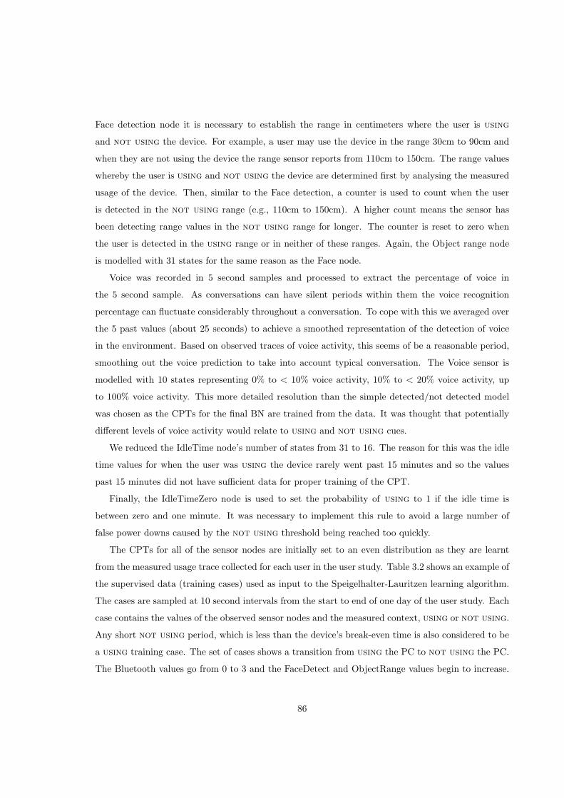
Face detection node it is necessary to establish the range in centimeters where the user is using
and not using the device. For example, a user may use the device in the range 30cm to 90cm and
when they are not using the device the range sensor reports from 110cm to 150cm. The range values
whereby the user is using and not using the device are determined first by analysing the measured
usage of the device. Then, similar to the Face detection, a counter is used to count when the user
is detected in the not using range (e.g., 110cm to 150cm). A higher count means the sensor has
been detecting range values in the not using range for longer. The counter is reset to zero when
the user is detected in the using range or in neither of these ranges. Again, the Object range node
is modelled with 31 states for the same reason as the Face node.
Voice was recorded in 5 second samples and processed to extract the percentage of voice in
the 5 second sample. As conversations can have silent periods within them the voice recognition
percentage can fluctuate considerably throughout a conversation. To cope with this we averaged over
the 5 past values (about 25 seconds) to achieve a smoothed representation of the detection of voice
in the environment. Based on observed traces of voice activity, this seems of be a reasonable period,
smoothing out the voice prediction to take into account typical conversation. The Voice sensor is
modelled with 10 states representing 0% to < 10% voice activity, 10% to < 20% voice activity, up
to 100% voice activity. This more detailed resolution than the simple detected/not detected model
was chosen as the CPTs for the final BN are trained from the data. It was thought that potentially
different levels of voice activity would relate to using and not using cues.
We reduced the IdleTime node’s number of states from 31 to 16. The reason for this was the idle
time values for when the user was using the device rarely went past 15 minutes and so the values
past 15 minutes did not have sufficient data for proper training of the CPT.
Finally, the IdleTimeZero node is used to set the probability of using to 1 if the idle time is
between zero and one minute. It was necessary to implement this rule to avoid a large number of
false power downs caused by the not using threshold being reached too quickly.
The CPTs for all of the sensor nodes are initially set to an even distribution as they are learnt
from the measured usage trace collected for each user in the user study. Table 3.2 shows an example of
the supervised data (training cases) used as input to the Speigelhalter-Lauritzen learning algorithm.
The cases are sampled at 10 second intervals from the start to end of one day of the user study. Each
case contains the values of the observed sensor nodes and the measured context, using or not using.
Any short not using period, which is less than the device’s break-even time is also considered to be
a using training case. The set of cases shows a transition from using the PC to not using the PC.
The Bluetooth values go from 0 to 3 and the FaceDetect and ObjectRange values begin to increase.
86

Table 3.2: Example BN training cases
No. IdleTime Bluetooth FaceDetect VoiceActivity ObjectRange IsNotUsing
1 * 0 2 * 1 Using
2 * 0 1 * 0 Using
3 * 0 1 * 0 Using
4 * 0 1 * 0 Using
5 * 0 0 * 0 Using
6 * 0 2 * 2 Using
7 * 1 4 * 4 *
8 * 2 6 * 5 *
9 * 3 8 * 7 *
10 * 3 10 * 9 *
11 * 3 12 * 11 *
12 1 3 14 * 12 *
13 1 3 16 * 14 NotUsing
14 1 3 18 * 16 NotUsing
15 1 3 20 * 18 NotUsing
16 1 3 22 * 19 NotUsing
17 1 3 24 * 21 NotUsing
18 2 0 25 * 0 NotUsing
19 2 0 27 * 1 NotUsing
20 2 0 29 * 3 NotUsing
The asterisks (*) represent values that are not to be included in the learning. These include idle time
values less than one minute, voice activity values of 0% and any cases where the value of using/not
using is not known. Given this supervised training data the expected probabilities of the CPTs are
estimated.
To give a concrete example of the learning theory explained in Section 3.6, we consider learning of
the CPTs for the Bluetooth node based on the set of cases given in Table 3.2. The Bluetooth node is
a multinomial variable with four values 0, 1, 2 and 3. For each state of the parent node IsNotUsing,
there is a Dirichilet distribution, F , that represents the expected probability of each of the Bluetooth
values, given the parent state. For example, given the user is using the PC we expect the probability
87

of the Bluetooth value 0 (i.e., detected) to be high. The distribution has four parameters a1, a2, a3
and a4 to represent the number of times each Bluetooth value is observed in the given parent state,
and the parameter N , which keeps a total count of the number of cases observed. The expected
probability for any of the Bluetooth values is given as E(Fk) = ak
N . Initially the expected probability
for all values in the Bluetooth node’s CPTs are evenly distributed with value 14 . In the first training
case, the parent state is using and the Bluetooth value is 0. Therefore the expected probability for
Bluetooth value 0 given using rises to 25 and the expected probabilites for the other values reduce
to 15 . By the sixth case the expected probability for Bluetooth value 0 given using rises to 7
10 and
the probability for the other values reduce to 110 . For the following six cases, the state of IsNotUsing
is not known and hence these cases cannot be learnt. The thirteenth training case is the first case
where the parent state is not using. Therefore the expected probability for Bluetooth value 3 given
not using rises to 25 . By the seventeenth case, this probability has risen to 6
9 . In the eighteenth case
the Bluetooth tag is detected again (value 0) but the user is still not using the device. Therefore the
expected probability for Bluetooth value 0 given not using rises to 210 . By the final case the expected
probabilities for Bluetooth values 0, 1, 2, 3 given not using are 412 , 1
12 , 112 and 6
12 respectively.
This has given a concrete example of how the case data is used for learning the CPTs. Example
CPTs for each of the sensor nodes, which have been trained on a full day of case data are described
in Section 4.1.
3.8.2.2 About to use
In the initial about to use model the device is powered up anytime the Bluetooth tag is detected.
This causes a problem when the device is put into standby and the Bluetooth tag is still being
found in the vicinity. The model was extended by adding the InStandbyBTFound node to model
this InStandbyFound (ISF) state. When in the ISF state the influence of the Bluetooth tag being
found is nullified (the probability of Bluetooth being found is 0.5 for both the not using (NU) and
about to use (ATU) cases). This prevents the presence of the Bluetooth tag causing the device to
be immediately powered up again. Only when the device powers down to standby and the tag is not
found (ISNF), will the device power up due to the Bluetooth tag being found again.
The about to use model needs to power up the device as quickly as possibly to avoid the user
experiencing any resume-time delay. Therefore it is not necessary to extend the Bluetooth node to
record recent history as it needs to power up the first time the Bluetooth tag is detected. This
requirement to power up quickly causes a problem for the Face and Object range sensors, as they are
more prone to reporting false detections. When either of the sensors falsely detected a face or object,
88

P(NU) P(ATU)
0.5 0.5
Bluetooth
IsAboutToUse
InStandbyBTFound
P(ISF) P(NISF)
0.5 0.5
NU NU ATU ATU
Bluetooth ISF ISNF ISF ISNF
P(Found) 0.5 0.5 0.5 0.9
P(NotFound) 0.5 0.5 0.5 0.1
Figure 3.18: Final BN about to use model
the device was powered up. Therefore, in the final version of the about to use model the Face and
Object range sensors were not used as they caused too many false power ups. The Voice sensor was
not used either as it is not a good indicator of about to use. The CPTs for the about to use
model are fixed (i.e., not learnt from the data) as shown in Figure 3.18.
3.8.3 DBN models
Finally, a dynamic Bayesian model was designed to investigate if this technique could improve on the
performance of the final Bayesian model, in particular, for devices with relatively long break-even
times.
3.8.3.1 Not using
The DBN not using model is a simple extension of the final BN model to include a number of time
slices in the future. The structure of the nodes is the same within a time slice and the transition arcs
link a node in the previous time slice to the corresponding node in the next time slice (see Figure
3.19). This rolled out network is effectively a standard Bayesian network and the techniques for
89

inference updating and learning are the same. The IdleTimeZero node is only needed at the final
IsNotUsing6 node to implement the rule of using if the idle time is less than one minute. The size
of the time step between time slices is calculated as the break-even time of the device divided by
the number of time slices (6). Therefore, if the break-even time is one minute, the time step is 10
seconds; if the break-even is 6 minutes, the time step is one minute. This gives the prediction of the
not using probability for the IsNotUsing6 query node to be the break-even time in the future for
the device.
IdleTimeZero
Bluetooth1
IdleTime1
Face1
Object1
Voice1
IsNotUsing1
Bluetooth0
IdleTime0
Face0
Object0
Voice0
IsNotUsing0
Bluetooth6
IdleTime6
Face6
Object6
Voice6
IsNotUsing6
Figure 3.19: DBN not using model
Again, as for the learning of the BN model, the CPTs for all sensor nodes are initially set to an
even distribution. The training cases are sampled at the given DBN time step (e.g., 10 seconds, 1
minute) from the start to end of one day of the user study. The training cases for the DBN are much
wider as a value is needed for each sensor node in the each of the time slices. Table 3.3 shows an
example set of training cases for the six time slices of the Bluetooth nodes and the IsNotUsing6 node.
A complete case would include all of the nodes in each of the time slices. The example set of cases
shows the Bluetooth nodes values changing from detected (0) to not detected (3) as the IsNotUsing6node transitions from using to not using the PC. Training the DBN model with the complete case
data learns both the conditional probabilities of the nodes (e.g., the probable values of BT6 given the
IsNotUsing6 state) and the transition probabilities between nodes in the subsequent time slice (e.g.,
the probable values of BT6 given the value of BT5).
90
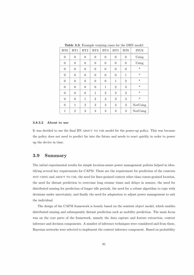
Table 3.3: Example training cases for the DBN model
BT0 BT1 BT2 BT3 BT4 BT5 BT6 INU6
0 0 0 0 0 0 0 Using
0 0 0 0 0 0 0 Using
0 0 0 0 0 0 0 *
0 0 0 0 0 0 1 *
0 0 0 0 0 1 2 *
0 0 0 0 1 2 3 *
0 0 0 1 2 3 3 *
0 0 1 2 3 3 3 *
0 1 2 3 3 3 3 NotUsing
1 2 3 3 3 3 3 NotUsing
3.8.3.2 About to use
It was decided to use the final BN about to use model for the power-up policy. This was because
the policy does not need to predict far into the future and needs to react quickly in order to power
up the device in time.
3.9 Summary
The initial experimental results for simple location-aware power management policies helped in iden-
tifying several key requirements for CAPM. These are the requirement for prediction of the contexts
not using and about to use, the need for finer-grained context other than coarse-grained location,
the need for distant prediction to overcome long resume times and delays in sensors, the need for
distributed sensing for prediction of longer idle periods, the need for a robust algorithm to cope with
decisions under uncertainty, and finally the need for adaptation to adjust power management to suit
the individual.
The design of the CAPM framework is loosely based on the sentient object model, which enables
distributed sensing and subsequently distant prediction such as mobility prediction. The main focus
was on the core parts of the framework, namely the data capture and feature extraction, context
inference and decision components. A number of inference techniques were considered and from these,
Bayesian networks were selected to implement the context inference component. Based on probability
91

theory, they enable inference based on uncertain data and provide mechanisms for learning to adapt
to users’ behaviours. The set of sensors selected for CAPM of desktop PCs were a Bluetooth tag,
web camera, microphone, ultra-sonic object range sensor and idle time from the mouse and keyboard
input events. The design of the networks involved substantial trial and error modelling until a final
BN model was settled on. The evolution of the design of the Bayesian networks is detailed. Finally, a
dynamic Bayesian model was also designed so its performance could be compared to the BN model’s
performance.
The next chapter details the implementation of the CAPM framework for power management of
desktop PCs and their displays.
92

Chapter 4
Implementation
This chapter describes the implementation of the CAPM framework for power management of desk-
top PCs and their display units in an office environment. Figure 4.1 shows the structure of the
implementation.
ConsumePowermanagementAPI
Datacapture &
featureextraction
Contextinference
Decisionmaking
Bluetooth
Video
Sound
Ultrasonicrange
Time of day
Figure 4.1: Software structure
We first describe the sensor hardware and software used for data capture and feature extraction.
Significant characteristics of each of the sensors are also highlighted. We then go on to describe the
choice of Bayesian software used for implementing the Bayesian inference and learning, which is the
core of the CAPM framework. The CAPM implementation is divided into two parts, (a) the runtime
(on-line) CAPM implementation, and (b) the off-line CAPM evaluation software. The runtime CAPM
software provides the actual implementation of the BN policies, whereas the off-line CAPM software
is used for the evaluation of the user study. It records the sensor data and user’s usage of the PC,
and subsequently simulates the range of BN policies for evaluation purposes. The runtime CAPM
93

implementation is first described, including the Windows power management functionality. Finally,
the CAPM evaluation software is described.
4.1 Sensors
The hardware and software implementation of the sensors is detailed in the following sections. The
development platform used was the Microsoft platform SDK, Windows server 2003 family, and the
code was compiled for Windows XP. The Bluetooth sensor required the use of service pack 2. As de-
scribed in Chapter 3 the sensors used in the CAPM implementation were system idle time, Bluetooth
presence, face detection, voice activity detection, and object range detection.
4.1.1 System idle time
System idle time is the amount of time since the user last caused an input event (e.g., moved the mouse
or touched the keyboard). The Windows GetTickCount() method returns the amount of time, in
milliseconds, that has passed since the last time the computer was started. This is called the tick count
of the computer and represents how long the computer has been running. The GetLastInputInfo()
method retrieves the tick count of the last input event into the LASTINPUTINFO structure. The
IdleTimeGetState() method simply subtracts this value from the current tick count to get the idle
time in seconds (see Listing 4.1). The tick count loops every 49.7 days, which is not an issue for this
experiment. The energy cost of this sensor information is not measurable and is assumed to be zero.
Listing 4.1: System idle time
1 int IdleTimeGetState ( ) {
2 LASTINPUTINFO l p i ;
3 l p i . cbS ize = s izeof ( l p i ) ;
4 // Get the TickCount ( time ) o f the l a s t user input
5 GetLastInputInfo(& l p i ) ;
6 // Return the curren t TickCount − l a s t user input TickCount
7 return ( GetTickCount ( ) − l p i . dwTime) / (1000) ;
8 }
In the designed Bayesian network, the idle time node represents the idle time in one minute bins
from 0 to 1 minute, up to 15 minutes and greater. Figure 4.2 shows an example of the learned
conditional probability tables (CPTs) for the idle time node. Figure (a) shows the probability of an
94

0
0.1
0.2
0.3
0.4
0.5
0.6
0.7
0.8
0.9
1
0 1 2 3 4 5 6 7 8 9 10 11 12 13 14 15
Idle time
prob
abili
ty
(a) Probability given Not Using
0
0.1
0.2
0.3
0.4
0.5
0.6
0.7
0.8
0.9
1
0 1 2 3 4 5 6 7 8 9 10 11 12 13 14 15
Idle time
prob
abili
ty
(b) Probability given Using
Figure 4.2: Idle time CPTs
0
0.1
0.2
0.3
0.4
0.5
0.6
0.7
0.8
0.9
1
0 1 2 3 4 5 6 7 8 9 10 11 12 13 14 15
Idle Time
prob
abili
ty
Figure 4.3: Inferred probability of not using
idle time given the user is not using the device and Figure (b) gives the probability of an idle time
given the user is using the device. The 0 to 1 minute period has been excluded from the learning as
for this value the probability of using is explicitly set to one. (The IdleTimeZero node ensures that
using = 1 when the idle time is less than 1 minute.)
Figure 4.3 shows the inferred probability of not using for the given idle times. The probability of
not using rises sharply after the 1 to 2 minute period (from 0.06 to 0.44) and then stabilises around
0.5. It drops off again after the 9 to 10 minute period and finally rises sharply to 0.96 in the 15-
minute-and-greater period. The fluctuation of the probability is due to the lack of cases for learning
in the higher idle time periods and the sharp rise at the end is because the 15-minute-and-greater
period encompasses all cases greater than 15 minutes.
95

Sparsity of data for learning is a common issue for learning of parameters. Also, the discretisation
of continuous values (e.g., idle time) cause problems when upper bound limits are set. Applying a
smoothing function to the idle time CPTs could reduce the fluctuation in the graph of not using
probability versus idle time and may be more appropriate. For example, an exponential function
could possibly be used to ensure the idle time CPTs transition smoothly from the 0 to 1 minute to
the 15-minute-and-greater period. This would need to be explored further as future work.
4.1.2 Bluetooth presence
The initial experimental trials used Bluetooth-enabled mobile phones as location/presence tags. For
the larger user study we purchased dedicated Bluetooth tags as not enough of the population currently
have Bluetooth-enabled phones. The tags we choose were Bluelon BodyTags 002 [5], which have a
Class I (100mW) radio with a range of up to 100m. For the experiment, the power was tuned down
to 2.5mW (giving a range of 10m), which is the range of the Class II radios found in mobile phones.
All Bluetooth devices have a unique device address, and a clock to enable frequency hopping.
A network (piconet) of Bluetooth devices can be established with one device as the master and the
rest as slave devices. There are two possible methods of determining whether a Bluetooth device is
present, either by using device discovery to attempt to discover the device or, if the device’s address
is known, a faster direct attempt to connect to that device can be made. Both of these protocols are
implemented in the link controller layer. In an error-free environment the worst case time to discover
a device is around 10s [8]. Device discovery is the method we used in the initial experimental trial
for detecting the presence of the mobile phone.
We improved on this time by using the connection protocol to detect whether the device is present
or not. To initiate a connection the master device enters the paging mode, whereby it transmits the
slave device’s address on a 32 channel frequency hop sequence. This paging device hops at a fast
rate, one hop every 312.5µs. Meanwhile, the slave device should be in the page scan mode, listening
for connections. This scanning device hops over the same channels at a slow rate of one hop every
40ms. When the paging device catches up with the scanning device, the slave hears its address being
broadcast and then replies to the master. Once this handshaking has been achieved, the connection is
established. For the experiment, the desktop PC acts as the master device continually attempting to
connect to the PC owner’s slave Bluetooth tag. The Windows Winsock API was used to implement
the connection with the tag. The WSALookupServiceBegin function attempts to connect to the given
Bluetooth tag address. If the connection succeeds then we determine the Bluetooth tag is present.
If the connection fails then either the Bluetooth tag is not there or the connection protocol failed to
96

0
0.1
0.2
0.3
0.4
0.5
0.6
0.7
0.8
0.9
1
0 1 2 3
Bluetooth count
prob
abili
ty
(a) Probability given Not Using
0
0.1
0.2
0.3
0.4
0.5
0.6
0.7
0.8
0.9
1
0 1 2 3
Bluetooth count
prob
abili
ty
(b) Probability given Using
Figure 4.4: Bluetooth CPTs
0
0.1
0.2
0.3
0.4
0.5
0.6
0.7
0.8
0.9
1
0 1 2 3
Bluetooth count
prob
abili
ty
Figure 4.5: Inferred probability of not using
connect to the tag, which sometimes happens.
A series of experiments were conducted for the Bluetooth connection. The average time to make a
new connection to a Bluetooth tag was measured to be between 1 and 2 seconds. When the Bluetooth
tag was not there the time it took for the connection to timeout was measured to be between 5 to
6 seconds. The connection error rate is the percentage of times the connection fails to connect with
the tag when the tag is present. This was measured by leaving a tag in close proximity (20cm) for a
4 hour period. The error rate for not detecting the tag once was 14.05%; not detecting twice in a row
was 0.73%; not detecting three times in a row was 0.17% and there were no cases of not detecting
four times in a row. Based on this connection error rate the Bluetooth node was modelled to have
three not detected states.
97

Figure 4.4 shows the Bluetooth CPTs for a typical user. When they are not using the PC (Figure
(a)), the tag is detected with probability 0.14 and not detected (value 3) with probability 0.85. When
they are using the PC (Figure (b)) the Bluetooth tag is nearly always detected (value 0). Figure
4.5 shows the inferred probability of not using rising as the Bluetooth count goes from 0 to 3.
All values of the Bluetooth count are well sampled and the smooth transition of the not using
probability models well the increasing certainty that the user is not there and therefore not using
the PC.
4.1.3 Face detection
A web camera (initially a Creative USB 2.0 camera) was used to capture video at 30 frames per second
(fps) and 640x480 resolution. The general-purpose face detection algorithm is a Haar-like training
classifier, which is implemented by the open computer vision library (OpenCV). This open source
library is a collection of algorithms for basic computer vision problems and was originally developed
by Intel [30].
Face detection is a relatively difficult object detection task due to the large variety of possible face
instances, e.g., faces may be slightly rotated or tilted, some people wear glasses, some have beards
or moustaches, and often part of the face may be in shadow. Statistical model-based training can
be used to cope with this large variety. The Haar-training classifier used by OpenCV was originally
developed by Viola and Jones [64] and is described in [6]. The method uses simple geometric features
(the features are computed in a similar way to coefficients in Haar wavelet transforms) and a cascade
of boosted tree classfiers as the statistical model. Face detection is done by sliding a fixed size window
across the image and classifying whether the candidate image in the window looks like a face or not.
To detect faces of different sizes, the image is scaled. In the algorithm, fourteen Haar-like features
are used (see Figure 4.6).
Each feature is described by its black and white template, its relative coordinate in the window,
and its size. For example, in many faces eyes are darker than the surrounding regions so feature 3 (a)
centered at one of the eyes and properly scaled will likely give a large feature value. The computed
feature value xi is fed into a very simple classfier fi ={
+1, x≥t−1, x<t , where t is a given threshold value, +1
means face detected, and -1 means not detected. A more robust “boosted” classifier is then built from
the set of “weak”classfiers as a weighted sum of the weak classifiers: F = sign(c1f1+c2f2+...+cnfn).
The more classifiers included in the sum the better the prediction of the boosted classifier. To manage
the computational complexity, Viola suggested using a set of boosted classifiers Fk with increasing
complexity. The image is then sequentially applied to the set of classifiers in increasing order. In
98

(a) (b) (c) (d)
(a) (b) (c) (d) (e) (f) (g) (h)
(a) (b)
1. Line features
2. Edge features
3. Center surround features
Figure 4.6: The Haar-like features
experiments, 70-80% of candidate images get rejected in the first two stages, leaving the final more
complex stages to handle candidate images that could be faces. The initial window size for detecting
faces was set to 100x100 pixels to avoid detecting small scale faces, (i.e., in the distance). A nice
property of this algorithm is that there is no need to train the classifier to a specific user’s face.
The positioning of the camera was either on top of the user’s monitor or below it, depending on
the monitor’s height. In one case the face detection did not work as the particular user had their head
very close to the monitor, so it was not possible to get a front on image of the face for recognition.
Figure 4.7 shows 4 sample images of the face detection (where a red box means the face is detected).
It shows that the face needs to be looking straight at the screen for it to be detected. Sometimes a
false detection of a face in the background can occur.
The CPU consumption of the Creative camera was very high for image capture, at around 30%
of the CPU. We found a cheaper Trust USB 2.0 camera, which consumed much fewer CPU resources
(8% CPU) to run the user trials. To estimate the potential error rate of the camera we conducted a
simple experiment, whereby a user constantly looked at the screen for an hour (i.e., their face position
was fixed for this period). From this, the error rate of the face detection was estimated to be 1.58%,
(i.e., the face was not detected once in every 63 samples). This error rate increases in circumstances
of poor lighting or when the camera positioning is not suited to the user’s position.
Figure 4.8 shows typical learned CPTs for the face detection node. Given the user is not using
the PC, the most probable face detection value is 30-and-greater (Figure (a)). If the user is using
the PC the most probable values are between 0 to 4 face detect counts (Figure (b)). This models the
99

Figure 4.7: Face detection
fact that the face is not always detected during the use of the PC.
4.1.4 Voice activity detection
A standard, cheap PC microphone (LabTec AM-22) and standard PC sound card were used for the
sound recording. The voice activity detection (speech detection) algorithm is a simple energy and
periodicity algorithm commonly used for end pointing in speech recognition algorithms [53]. End
pointing is used to seperate acoustic events of interest (i.e., speech) from the background signal.
Rabiner states there are three factors that make the task of speech detection difficult [53]. The first
is the extra sound made by a speaker such as lip smacks, heavy breathing, mouth clicks, and pops.
The second is due to difficult environmental conditions such as noisy backgrounds (e.g., due to fans,
machinery running), non-stationary environments (e.g., door slams, trains passing by, car horns), and
in hostile circumstances when the speaker is stressed (e.g., when navigating an airplane). Rabiner
states that some of these interfering signals produce as much speech like quality as the desired speech
signal itself, making accurate speech detection quite difficult. The final source of difficulty is the
100

0
0.1
0.2
0.3
0.4
0.5
0.6
0.7
0.8
0.9
1
0 2 4 6 8 10 12 14 16 18 20 22 24 26 28 30
Face detect count
prob
abili
ty
(a) Probability given Not Using
0
0.1
0.2
0.3
0.4
0.5
0.6
0.7
0.8
0.9
1
0 2 4 6 8 10 12 14 16 18 20 22 24 26 28 30
Face detect count
prob
abili
ty
(b) Probability given Using
Figure 4.8: Face detection CPTs
distortion introduced by the transmission medium itself. For signals with a stationary and low noise
background, a straight-forward energy-level algorithm produces reasonably good accuracy.
The algorithm we selected is from Intel’s integrated performance primitives (IPP) toolkit [29].
The toolkit provides a library of optimised functions for audio, video, speech, computer vision, image
and signal processing1. The approach involves measuring the short-time energy level of the sound
sample and the periodicity of the sample to filter unwanted noise in the background. Speech signals
are periodic in nature, which distinguishes them from the background noise.
The voice activity detection code records the sound from the microphone every 5 seconds as a pulse
code modulated (PCM) file. The PCM file is processed by the IPP speech detection algorithm and it
returns the percentage of active sample windows in the sound recording. This gives the percentage
of voice activity that occurred in the last 5 seconds of recording.
The voice activity detection was initially tested with a user speaking directly into the microphone.
For the experiment, the microphone was positioned hanging above the user’s work station. This
reduced the performance of the algorithm as the microphone was further from the speech. A possible
solution to this could have been to use better quality microphones, which are more sensitive.
Figure 4.9 shows typical CPTs for the voice activity. There is no significant difference between the
not using and using CPTs, which means that in both contexts the voice activity is quite similar.
This suggests that the voice activity information was not a good indicator for inferring the contexts
using and not using.1Intel’s OpenCV library can use IPP for optimised performance.
101

0
0.1
0.2
0.3
0.4
0.5
0.6
0.7
0.8
0.9
1
0 10 20 30 40 50 60 70 80 90
Voice activity
prob
abili
ty
(a) Probability given Not Using
0
0.1
0.2
0.3
0.4
0.5
0.6
0.7
0.8
0.9
1
0 10 20 30 40 50 60 70 80 90
Voice activity
prob
abili
ty
(b) Probability given Using
Figure 4.9: Voice activity CPTs
4.1.5 Object range detection
An ultrasonic range-finding sensor was used to determine the distance to the nearest object in front
of the PC. The sensor works by transmitting a short burst of high-frequency (ultrasonic) sound into
the environment and measuring the time taken for the reflected echo to return to the receiver. The
distance is calculated by simply dividing the echo time by the speed of sound. The accuracy of an
ultrasonic sensor varies as the speed of sound changes depending on environmental factors such as
temperature, air pressure, humididty, and acoustic interference [59].
We used an SRF08 ultrasonic sensor, which has a range of about 6 metres. The sensor is connected
to an OOPIC-R micro-controller via an IC2 bus. The micro-controller sends the sensor a signal to
transmit, which causes the sensor to transmit the ultrasonic beam. The sensor then listens for an
echo for a period up to 65ms (i.e., corresponding to the maximum range of 6m). Once ranging is
complete, the measured range can be read from the sensor. The micro-controller then outputs this
range reading to its serial port, from which it can be read by the PC.
In the experiment the sensor was positioned at the top of the monitor and its beam angled to
pick up the head of the user when they were sitting at the PC and facing the monitor. This required
a certain amount of calibration and in some cases it was difficult to pick up the user’s head without
picking up the back of a high office chair when the user was not there. Another difficult case was when
the user was turned around 180 degrees talking to a colleague as the back of their head was being
picked up at a similar distance to when they were using the PC. A possible improvement could be to
use an infra-red sensor, which can also distinguish body heat. This would eliminate the more common
problem of picking up the back of a high chair. Infra-red sensors are not as accurate as ultrasonic
102

0
0.1
0.2
0.3
0.4
0.5
0.6
0.7
0.8
0.9
1
10 30 50 70 90 110
130
150
170
190
210
object range (cm)
prob
abili
ty
(a) Probability given Not Using
0
0.1
0.2
0.3
0.4
0.5
0.6
0.7
0.8
0.9
1
10 30 50 70 90 110
130
150
170
190
210
Object range (cm)
prob
abili
ty
(b) Probability given Using
Figure 4.10: Typical using/not using object ranges
ones, so a possibility might be to use both sensors [25]. The reliability of the range detection was
estimated by placing an object 6cm in front of the sensor and recording the measurements over an
hour. The measurements’ median and standard deviation were 5.88cm +/- 0.80cm for the 6cm object.
The sensor more commonly over-estimated the distance with the largest reading being 12cm.
The object range detection node was designed to count when the user was last detected in the
using object range. The using/not using ranges were different for each user and were determined
based on the object range values and the measured usage trace. Figure 4.10 shows typical object
range values given the user is not using (Figure (a)) and using (Figure (b)) the PC. The ranges
are well seperated with the using range from 30cm to 80cm and the not using range from 90cm to
160cm.
However, for some users the separation of ranges was not so clean and the using and not using
ranges coincided. Figure 4.11 shows the using range coinciding with the first part of the not using
range from 90cm to 120cm. In these cases where there is some overlap, the using range is given
precedence (e.g., 40cm to 120cm) and the not using range is reduced to exclude any overlap (e.g.,
130cm to 150cm). This means that in the overlap range it is not possible to classify whether the user
is in the using or not using range and the safest option is to assume they are using to avoid a false
prediction of not using the device.
Once the using/not using ranges are known the object range values can be converted into object
detection counts. The counter is incremented if the object range is in the not using range and reset
to 0 if it is in the using range. This gives a history of when an object was last detected in the using
range. Figure 4.12 shows typical CPTs for the object detection count. Given the user is not using
103

0
0.1
0.2
0.3
0.4
0.5
0.6
0.7
0.8
0.9
1
10 30 50 70 90 110
130
150
170
190
210
Object range (cm)
prob
abili
ty
(a) Probability given Not Using
0
0.1
0.2
0.3
0.4
0.5
0.6
0.7
0.8
0.9
1
10 30 50 70 90 110
130
150
170
190
210
Object range (cm)
prob
abili
ty
(b) Probability given Using
Figure 4.11: Coinciding using/not using object ranges
0
0.1
0.2
0.3
0.4
0.5
0.6
0.7
0.8
0.9
1
0 2 4 6 8 10 12 14 16 18 20 22 24 26 28 30
Object detect count
prob
abili
ty
(a) Probability given Not Using
0
0.1
0.2
0.3
0.4
0.5
0.6
0.7
0.8
0.9
1
0 2 4 6 8 10 12 14 16 18 20 22 24 26 28 30
Object detect count
prob
abili
ty
(b) Probability given Using
Figure 4.12: Object detection CPTs
the PC the most probable object detection count is 30-and-greater (Figure (a)). If the user is using
the PC the most probable object detection count is 0 (Figure (b)).
4.1.6 Sensor power consumption
The power consumption of each sensor was measured to be the difference between the power con-
sumption of the base PC and the power consumed when the individual sensor was operating. A power
monitor was used to accurately measure the energy consumption in Watt hours (Wh) over a 12 hour
period for the base PC and the PC with each of the individual sensors. The measurements were each
repeated 7 times to estimate the possible variance in the energy consumption. The base PC had a
freshly installed operating system with no applications or anti-virus software installed. It included a
104

Bluetooth radio, web camera, and microphone hardware as it is assumed this hardware will become
standard for a PC. Figure 4.13 shows the average power of each of the sensors (i.e., the difference of
power consumed when the sensor was operating and the power of the base PC).
Figure 4.13: Energy consumption of sensors
The average power of the Bluetooth presence detection is estimated at 0.41W +/- 0.19W. This
is based on a sample rate of attempting to connect once every 5 seconds and the tag being present
during normal office usage (i.e., for several periods during the day the tag was not present). It was
also necessary to estimate the energy consumed by recharging the Bluetooth tag. The power of the
charger is 1.03W and it was estimated that 3 hours of charging was necessary for the tag to last the
5 day trial period. Therefore the estimated energy consumption of recharging the Bluetooth tag is
0.62Wh per day, which is added to the energy cost of the Bluetooth presence detection.
The average power of the face detection was estimated at 2.47W +/- 0.22W above the base PC.
This is based on a sample rate of face detection once every 5 seconds. The power of the face detection
is significantly higher than the other sensors and is due to the large amount of processing needed to
perform the face detection algorithm. The average power of the voice activity detection is estimated
at 0.78W +/- 0.40 W. Again, the sample rate is once every 5 seconds but the data processing required
is less than the face detection.
The average power of the object range detection was divided into the power consumed by polling
105

the sensor for readings and the power consumed by the sensor itself. The measurements in Figure
4.13 show the power consumed by polling the sensor to be slightly less than that of the base PC,
which was unusual. We re-measured the base PC and found its power to be the same. We concluded
that the wall-powered OOPIC micro-controller might influence the base PC energy reading and that
the power consumed by reading the RS232 port once every 5 seconds is negligible. The average power
of the SRF08 sensor was measured by measuring the energy consumption of the power supply and
OOPIC micro-controller (over a one hour period) and comparing this with the energy consumption
when the SRF08 sensor was connected. The power difference was measured to be 0.10W +/- 0.03W
(i.e., from 0.07W to 0.13W) for the sensor. A technical specification of the sensor is given by Robot
Electronics [21]. Their measurements state the average current of the sensor in ranging is 12mA and
in standby is 3mA. The sensor ranges for 65ms and is in standby for 1s (the polling frequency was
set to 1s). These figures give the total average power to be 0.02W for the sensor. We took the figure
of 0.07W, which is at the lower end of the measured power, as the estimated average power of the
object range sensor.
4.2 BN software selection
This section defines the general requirements for a Bayesian network tool for CAPM. Most of the
information presented derives from Kevin Murphy’s web page [44] and Appendix B of [35].
4.2.1 Requirements
The general requirements were listed as:
Must
1. support continuous nodes (i.e., continuous-valued variables such as time).
2. support parameter learning (or allow it to be provided).
3. support dynamic BNs.
4. be executable on Windows, Unix, Mac OSX and also other non-standard embedded processors
(for CAPM of other office devices).
5. have an API.
6. support decision networks (or allow it to be provided).
106

Should
1. have good documentation.
2. have source code available and preferably in C, enabling pruning of code. This enables the code
base to be reduced in size for embedded platforms.
3. have a graphical interface for creating networks.
Could
1. support structure learning (i.e., the dependency arcs between nodes in a network).
The main driver behind this set of requirements was the need for a tool that could be used to build
a runtime CAPM implementation that could be executed on users’ PCs.
4.2.2 Tool selection
Based on the above requirements a set of seven possible tools was evaluated. Table 4.1 details the
name, authors, availability of source code, availability of an application programming interface, and
the set of execution environments supported (Windows, Unix, Macintosh, Embedded).
Table 4.1: Comparison of BN tools
Name Authors Source API Execution
Hugin Expert U. Aarhus None Yes Win
Netica Norsys None Yes Win, Unix, Mac, Embed
Genie (SMILE) U. Pittsburgh None Yes Win, Unix
Probabilistic Networks Library (PNL) Intel Research C++ Yes Win, Unix
Bayes Net Toolbox (BNT) Murphy Matlab, C Yes Win, Unix, Mac
Java Bayes Cozman (CMU) Java Yes Win, Unix, Mac
Bayesian Filtering Library (BFL) Klaas Gadeyne C++ Yes Win, Unix, Mac, Embed
The closed source tools Hugin Expert, Netica and Genie (SMILE), have a wide range of func-
tionality and comprehensive documentation. Hugin and Genie have the advantage of being closely
connected to BN research groups and implement more advanced inference algorithms. However, Ge-
nie (being non-commercial) has less functionality, for example, parameter learning is currently being
implemented, whereas, Hugin has structure learning. Genie can read both Hugin and Netica file
107

formats. Netica is a lighter weight implementation, which uses the standard junction tree inference
algorithm and a number of parameter learning algorithms. It is robust, capable of being embedded
(using only the standard C library) and provides for real-time requirements (i.e., all functions take
a predictable amount of time to complete). The open source tools PNL, BNT, Java Bayes and BFL
may lack finish, but make the source code available. Of these tools BFL is out of scope as it only
supports dynamic BNs and BNT is out of scope as it requires MatLab for execution. PNL has more
functionality than Java Bayes and is implemented in C++. We compared Netica and PNL by writing
a simple WaterSprinkler example for both. Netica has quite a simple well-documented API which was
easy to use but potentially less flexible. PNL development is a bit more complex but also possibly
more flexible. We decided to go with Netica and if further functionality was needed through access
to the code base, we could progress to PNL.
4.2.3 Netica
Netica is oriented towards commercial use. Versions of the Netica API are available for Microsoft
Windows (95/NT4 to XP), Linux, Sun Sparc, Macintosh (OS 6 to OS-X), Silicon Graphics and DOS.
Each of these has an identical interface, so code can be moved easily between platforms. They also
provide a service for building custom APIs to suit embedded platforms. There are two versions of
the API. The Java API gives the full functionality of Netica in an easy-to-program object-oriented
style. The C API is compact and fast, and is suitable for embedded systems. Each API comes with
good documentation including example programs and detailed descriptions of each function. The C
API does not require any library other than the Standard C library. The Java API does not require
any Java packages other than those that come with a standard Java 2 environment.
The network supports continuous nodes by allowing controlled discretisation. This is a simple
solution to handling continuous data (e.g., time) but does cause some modelling problems. For exam-
ple, a limit on the range of the data needs to be selected (see Section 4.1.1). The parameter learning
algorithms include the Spiegelhalter and Lauritzen parametrisation algorithm, and the expectation
maximization algorithm, which are sufficient for our current requirements. Structure learning is not
supported but this functionality could be provided by another tool dedicated to structure learning.
The latest version of Netica provides support for dynamic Bayesian networks through their “time-
delay” links. This allows the programmer to build a BN with time-delay links and then “roll out”
the network to include the required time slices. Decision networks are provided for and can support
multiple decision nodes. This enables multi-stage decision problems, where later decisions depend on
the outcomes of earlier ones.
108

The Netica inference engine has been optimised for speed for real-time performance. The network
is compiled into a junction tree of cliques for fast probabilistic reasoning. Programs that use the API
completely control the inference engine. They state that “no API function will ever take any action
until called. The API will not do any I/O unless requested to, and all functions take a predictable
amount of time before returning. Also, a limit may be set on the maximum amount of memory that
Netica will use.”
The graphical inteface is invaluable for making quick prototypes and experimenting with different
structures, learning and inference. The source code is not available as it is a commercial product. A
free version has the entire set of functionality as the licensed version but is limited in the size of net
that can be constructed.
4.3 Runtime (on-line) CAPM implementation
Two versions of the CAPM framework were implemented. The first runtime (on-line) implementation
was used for executing the CAPM policies during the runtime operation of a user’s PC. The second off-
line implementation was used for evaluation of the set of power management policies and is discussed
in Section 4.4.
The runtime version of CAPM was implemented as a background Windows service and uses
Netica’s C API to perform the inference using the Bayesian networks. This implementation was only
used for power management of the PC’s display as the power-up part of CAPM could not execute if
the PC itself was in standby. Additional hardware would be needed to implement automated power
up for the PC, or, as was the case with the SWOB policy, a remote server could be used.
The program sits in a loop continually polling the set of sensors for their current value. The
polling loop is divided into the two policies, power-down and power-up. If the PC’s display is on, the
power-down policy operates and the not using network is used to infer the probability of the user
not using the display. If the display is in standby, the power-up policy operates and the about to
use network is used to infer the probability of the user about to use the display. The Bayesian
networks use predefined CPTs and there is no on-line learning of the CPTs. On-line learning of the
CPTs is a possible area for future work. The decision making policy is a simple threshold decision. If
the probability of the given context is above the threshold then the appropriate power management
action (i.e., power down or power up) is performed.
We needed to determine whether the Bayesian inference consumed a significant amount of energy
or not. The energy consumption of the base PC was measured with the CAPM service executing
109

the full BN policy (i.e., Idle time, Bluetooth, Object range, Face detect, Voice activity). The actual
sensors were not polled for data so the service was just executing the inference of the Bayesian
network, once every 5 seconds. The energy consumption data was measured over a 12 hour period
and compared to the base PC consumption. The average power was estimated at -0.26W +/- 0.56W,
(0.30W, -0.82W), which is not significantly above zero. We therefore regard the energy consumption
of the CAPM inference to be negligible.
The Windows user interface API provides the functionality to switch the display to standby and
back on again. Listing 4.2 details the display (monitor) power management code. The SendMessage
function simply broadcasts a SC MONITORPOWER message to power off and on the display. The
function’s final parameter is set to 2 for powering off and -1 for powering on the display. The energy
consumption of transitioning the display is assumed to be negligible.
Listing 4.2: CAPM
1 void MonitorSuspend (void ) {
2 SendMessage (HWND BROADCAST, WMSYSCOMMAND, (WPARAM)SC MONITORPOWER, 2) ;
3 }
4
5 void MonitorOn (void ) {
6 SendMessage (HWND BROADCAST, WMSYSCOMMAND, (WPARAM)SC MONITORPOWER, −1) ;
7 }
The Windows power management API provides the means to switch the PC to standby. The
SetSystemPowerState function attempts to place the PC into the standby state. When the fForce
parameter is set to FALSE, the function broadcasts a PBT APMQUERYSUSPEND event to each
application to request permission to suspend operation. As long as no application denies the request
to suspend, the PC is put into standby.
The transition energy consumption Te of switching the PC to standby and back on was measured
by switching the PC to standby 10 times in a one hour period. The steady state on (Op) and
standby (Sp) power was measured independently and the on (Os) and standby state (Ss) times were
measured through the event API. The actual measured energy consumption of 22.78Wh is the sum
of the transition energy plus the energy consumed in the on state and the energy consumed in the
standby state (i.e., 22.78Wh = 10xTe + OpxOs + SpxSs). From this equation, the transition energy
was estimated at 0.19Wh per transition. This energy is added to the energy consumption of the
evaluation policies.
110

4.4 Evaluation (off-line) CAPM implementation
The evaluation of the CAPM policies required another set of software for the purpose of data collection
and off-line simulation of the set of policy traces. Figure 4.14 shows the structure of the evaluation
software.
Consume
Datacapture &
featureextraction
Contextinference
Decisionmaking
Bluetooth
Video
Sound
Ultrasonicrange
Time of day
Analysis Results
Figure 4.14: Evaluation software structure
The physical sensor hardware and software providing the data capture and feature extraction is
the same as for the on-line implementation. The evaluation software is divided into the data-collection
stage, which collects all of the data during the running of the user trial, the simulation of the policies
based on the data collected, and finally, the analysis of the simulated policy traces.
4.4.1 Data collection
A set of Windows services were implemented for polling the sensors and writing the time-stamped
values to disk for subsequent processing. These services reused the sensor code from the CAPM
implementation above. The Bluetooth, FaceDetect, ObjectDetect and VoiceActivity services polled
their respective sensor once every 5 seconds and wrote the sensor value to disk. Furthermore, the
Bluetooth service displayed a warning message box to the user if they were detected using the PC
when the Bluetooth tag had not been found for 10 periods or more. This warning ensured that the
users had their Bluetooth tag with them and that it was switched on. The IdleTime service recorded
every idle period greater than 30 seconds to the Windows event log. The PowerEvent service reported
all power event changes (standby, resume, shut down, start up) to the event log.
Finally, in order to evaluate the policies it was necessary to determine when the user was actually
using and not using the PC, (i.e., the device usage). This was achieved by implementing the NotUsing
service that monitored the idle time and for any idle period greater than 60 seconds, it would display
111

a message box asking the user if they were still using the PC. If the user saw this message box and
determined they were still using the PC then they could simply move the mouse to make the box
disappear. If they were involved in some other activity and did not see the message box, then the
display was powered off, establishing that the user was not using the PC for this period. The display
off and display on events were recorded to the event log. This is a sensitive part of the evaluation
as the measurement has the potential to change the user’s normal behaviour. To further minimise
the potential for modifying the user behaviour, an additional rule was added, whereby if the face
was detected looking at the display the policy would not attempt to power off the display. This is
discussed further in Section 5.3.
4.4.2 Simulation of policies
A device model framework was designed and implemented to simulate the set of evaluation policies
based on the recorded set of sensor data and the recorded device usage. This framework was imple-
mented in Java and used Netica’s Java API to interact with the same Bayesian networks used for the
on-line CAPM. The code was divided into three packages, Device Model, Capm, and Capm Analysis.
The Device Model class structure is detailed in Figure 4.15.
DeviceFactory
UsageFactory
State
DataErrorExceptionDeviceDeviceUsage 11
Usage11
StateTime
StateTimeList11
0..*0..*
Figure 4.15: Device Model
The Device class models the power states of a device and the Usage class contains the complete list
of power-state transitions for a particular usage trace. The DeviceUsage class combines a particular
device and usage trace together. The DeviceUsage is then used to provide information on the trace,
such as its energy consumption, the number of false power downs, and the number of manual power
112

ups. There are two types of trace. The measured usage trace is the measured record of when the user
was using and not using the PC. All other traces are policy traces which record when the device was
powered down and up by a particular policy.
The Capm classes are detailed in Figure 4.16. The Monitor class contains the measured usage
trace and reports to the particular Simulation class if the device can be powered down or not. The
Simulation classes use the Monitor and the recorded sensor data to run through the trace from start
to finish and generate the simulated policy trace. The InferenceEngine class provides the interface
to the Netica inference engine and the LearnCases class, implements the learning of the Bayesian
network CPTs based on the training cases. The SimulationEnv class generates these training cases
from the sensor data and the measured usage trace.
SimulationEnv
DBN_PowerDownUpSimulation
SWOBSimulation
ThresholdSimulation
PowerDownUpSimulation
InferenceEngine
LearnCases
Monitor
Figure 4.16: CAPM simluation
The Capm Analysis package processes the simulated policy traces. All of the required evaluation
metrics (e.g., energy consumption, false power downs) are queried from the DeviceUsage class and
printed to a .csv file. The .csv file format enables the results to be imported into a statistical package
for further analysis and presentation.
4.5 Summary
This chapter described the sensors used for CAPM of desktop PCs in an office environment. It
highlights the issues with each of the sensors and their estimated energy consumption. The selection
of the BN tool was then described and the implementation of the on-line CAPM and off-line CAPM
evaluation software were described. The next chapter describes the user study and presents the full
evaluation of the CAPM policies.
113

Chapter 5
Evaluation
This chapter begins by outlining the objectives of the CAPM user study, i.e., the research questions
we are trying to answer. We then describe how the user study was designed to ensure that the analysis
of its results answered the research questions. The data collection and processing of the measured
usage trace is then discussed and the simulation of the policies is described in detail. Finally, the
evaluation metrics are described and the results from the simulation are presented and evaluated.
5.1 Objectives
The first objective of the user study is to evaluate the potential of context-aware power management
for devices in an office environment. The initial experiments highlighted the failing of a simple
location-aware policy (SWOB) for LightUse users (see Section 3.1.5). Adding further types of sensor
can potentially do better but there is a limit as sensors themselves consume energy. The evaluation
objectives were to establish:
1. What is the potential extra energy that can be saved beyond the simple SWOB policy?
2. How much extra energy do policies with additional sensors save?
3. What is the estimated energy cost of operating the sensors?
4. What is the estimated user-perceived performance for each policy?
Overall, we are trying to establish what granularity and what types of context are appropriate for
CAPM of office devices. The sensors explored are user presence based on Bluetooth detection (BT),
near presence based on ultrasonic object range detection (OR), face detection (FD), and voice activity
114

detection (VA). The devices we consider are desktop PCs and their display units. These devices
account for a significant proportion of the energy consumed by office devices [33] and they are possible
to analyse within a single user study. Also, the break-even times of the devices (1 and 5 minutes)
enable evaluation of policy performance over a range of break-even times.
The second objective is to evaluate whether dynamic Bayesian networks are better for implement-
ing context-aware power management than standard Bayesian networks. Also, several general issues
regarding the use of Bayesian networks for CAPM are highlighted.
5.2 Design of the CAPM user study
In order to make some general statements about power management of devices in an office environment
we performed the study on a representative sample of the office population. We defined the population
of the study to be all workers in an office environment that use a desktop PC.
The initial experimental trial (see Section 3.1.5) highlighted the variability of usage patterns and
hence performance of the policies across a small sample of users (4 in total). From this four user
types were identified: HeavyUse, LightUse, FrequentUse and InfrequentUse. The trial also showed
that the performance of the SWOB policy depends primarily on whether the user is LightUse or
HeavyUse. Hence, the study is focused on these two user types. The sample selection for the trial
was designed to choose as diverse a range of users as possible from the set of potential candidates,
in order to capture as broad a range of device usage and office environments as possible. This was
done by generating a list of office users that could feasibly be approached to conduct the trial. The
list included the academic, administrative and postgraduate staff of Trinity College and several office
users from outside the college. There were four sets of hardware available to enable running the user
trials in parallel. However, each user trial took one hour to setup, normally 9 days to collect 5 days
of data and there were invariably problems encountered along the way. Due to the time constraints
and effort needed for conducting the trials, the sample size was set at 20 users. The criteria used for
selection from the list of potential users were:
1. Random, even spread from different job functions.
2. Random, even spread from different office environments.
3. Random, even spread from single office users and open plan office users.
The constraining requirements were that the potential candidates had to have a relatively new PC
(less than 5 years old) running Windows XP, a single display unit, and they had to be the sole user
115

Table 5.1: Sample selection
User Job Office type Location
A lecturer single O’Reilly
B lecturer single Lloyd
C administration open-plan O’Reilly
D postgrad open-plan O’Reilly
E manager open-plan Westland row
F technician open-plan Lloyd
G technician open-plan Lloyd
H administration single O’Reilly
I lecturer single O’Reilly
J administration single O’Reilly
K postgrad open-plan Lloyd
L lecturer single O’Reilly
M administration open-plan O’Reilly
N system admin single O’Reilly
O postgrad open-plan Lloyd
P lecturer single Lloyd
Q programmer open-plan Digital hub
R lecturer single Parson’s building
S administration open-plan Merrion square
T postgrad single Westland row
of the PC. From the list of 33 candidates approached, 13 of them were rejected because they did not
meet the requirement; 5 did not have Windows XP, 2 used laptops, 2 were not comfortable with being
monitored, one was busy moving office and 3 of the PCs had software conflicts with the monitoring
services1. Table 5.1 details the spread of people that were selected for the trial based on job function,
office type and location.
The trial length was set to run for 5 working days. Based on initial results, we believed this would
give enough data for training and simulation of the policies. Idle period data was collected for several
weeks after each trial to enable evaluation of any side affects from the trial.1The PCs’ remotely-managed anti-virus detection software shutdown the monitoring services when it started its
daily execution.
116

In order to compare a range of sensors and policies for each user’s usage trace it was necessary to
collect all sensor data simultaneously as the user was using the PC during the trial and subsequently
run policy simulations on the real usage data. Hence, the trial is broken into a data collection and
processing phase, and a subsequent simulation phase.
5.3 Data collection and processing
As described in Section 4.4.1 the data was collected for all sensors every 5 seconds; each value was
date stamped and stored to file. Furthermore, all idle periods of 30 seconds or more and all power
events were logged to the Windows event log. The most difficult data to collect was the actual usage
of the display and PC, i.e., when the user was actually using or not using these devices. To measure
the actual usage, the not using service attempts to power off the user’s display if the PC has been
idle for greater than 60 seconds. The 60-second period of time attempts to balance accuracy against
the experiment causing excessive user disruption. A message box appears asking the user if they are
still using the PC; if they are the message box disappears by simply moving the mouse. This short
mouse input will be removed in the data processing as it would not have happened during normal
deivce usage. To reduce disruption further the service checks if a face is detected before displaying
the message box. If a face is detected consistently during this period we assume the user is using the
PC and the idle period extends until the face is not detected (i.e., no message box will be displayed
until the face is not detected). It is possible that the face detection is identifying some object other
than a face, but this is unlikely as, (i) the reliability of the face detection was estimated at 1.58%,
(ii) the PCs are single user, and (iii) the user had been inputting 60 seconds before.
We imagined the affect that the not using service may have on the users’ behaviour was that
they would tend to make more inputs than normal to stop the monitor being powered off. This would
lead to a higher frequency of short idle periods than usual occurring in the usage trace. For this
reason, idle period data was collected for several weeks after each trial. The evaluation of this affect
is detailed in Section 5.7.
The event logs are processed to create the measured device-usage trace, of when the user was
using and not using the display or PC. Such a trace is graphed in Figure 5.1 where the line at
level 8 represents using and level 1 represents not using the PC. The line at level 7 represents idle
periods that occurred when using the PC. There are periods in every trace where we don’t know
whether the user was using the PC or not. These are the idle periods before the service attempts
to power down the monitor. The user may or may not be using the device at this time. These idle
117

0
1
2
3
4
5
6
7
8
9
10
15:
00
:00
15:
01
:32
15:
03
:04
15:
04
:36
15:
06
:08
15:
07
:40
15:
09
:12
15:
10
:44
15:
12
:16
15:
13
:48
15:
15
:20
15:
16
:52
15:
18
:24
15:
19
:56
15:
21
:28
15:
23
:00
15:
24
:32
15:
26
:04
15:
27
:36
15:
29
:08
15:
30
:40
15:
32
:12
15:
33
:44
15:
35
:16
15:
36
:48
15:
38
:20
15:
39
:52
15:
41
:24
15:
42
:56
15:
44
:28
15:
46
:00
15:
47
:32
15:
49
:04
15:
50
:36
15:
52
:08
15:
53
:40
15:
55
:12
15:
56
:44
15:
58
:16
15:
59
:48
Figure 5.1: Measured device usage
periods are scanned for face detection events. If a face is detected, we assume the state is using (i.e.,
the user was looking at the display during this idle period). If a face is not detected, a don’t know
state is inserted to indicate that we don’t know whether the user was using the PC or not at this
time. This don’t know state is represented by a line at level 6.
5.4 Simulation of policy traces
All of the policy traces are generated from the measured usage trace. We assume the behaviour of all
the users is good in that they power down their PC when leaving the office for the evening. So, for
all traces the device is switched to off for the night time period. For all policies, the policy is allowed
to power down in the don’t know and not using states; attempting to power down when the user
is still using represents a false power down.
From the measured trace, it is straightforward to generate the estimated Oracle policy trace and
the AlwaysOn trace. The Oracle policy trace is generated by placing the device in its standby state for
all not using periods that are greater than the device break-even time. The solid line in Figure 5.2
represents the power downs and power ups of the Oracle policy and the dashed line is the measured
device usage. The AlwaysOn trace is generated by leaving the device on for the duration of the day.
The SWOB policy was generated by running through the measured trace at a 5 second time step.
The policy attempts to power down if the Bluetooth tag is not detected more than 5 times and the
118

0
1
2
3
4
5
6
7
8
9
10
15:0
0:0
0
15:0
1:3
2
15:0
3:0
4
15:0
4:3
6
15:0
6:0
8
15:0
7:4
0
15:0
9:1
2
15:1
0:4
4
15:1
2:1
6
15:1
3:4
8
15:1
5:2
0
15:1
6:5
2
15:1
8:2
4
15:1
9:5
6
15:2
1:2
8
15:2
3:0
0
15:2
4:3
2
15:2
6:0
4
15:2
7:3
6
15:2
9:0
8
15:3
0:4
0
15:3
2:1
2
15:3
3:4
4
15:3
5:1
6
15:3
6:4
8
15:3
8:2
0
15:3
9:5
2
15:4
1:2
4
15:4
2:5
6
15:4
4:2
8
15:4
6:0
0
15:4
7:3
2
15:4
9:0
4
15:5
0:3
6
15:5
2:0
8
15:5
3:4
0
15:5
5:1
2
15:5
6:4
4
15:5
8:1
6
15:5
9:4
8
Figure 5.2: Oracle versus Measured
current idle time is greater than 60 seconds. If the measured usage is still in the using state a false
power down is reported, otherwise the policy powers down the device. The policy powers up when it
detects the Bluetooth tag (see Figure 5.3).
The range of Threshold policy traces were generated by running through the measured trace at
a 5 second time step. If the current idle time was greater than the given threshold, then the policy
attempts to power down. There is no automated power up for the Threshold policies. Figure 5.4
shows the Threshold 5 policy powering down 5 minutes after an idle period begins.
The Bayesian policies require a learning stage and a simulation stage. To be rigorous, we employed
a five-fold cross-validation strategy to the learning and simulation of the policies [18]. This involves
training the model on one day of data and simulating for the other four days, and repeating this five
times, training on each of the days. The resulting values are then estimated as the average of the
five simulation results, giving a more robust analysis of the policies. It also enables us to look at
variability of performance across training days and simulation days.
The Bayesian models we chose to compare, were idle time (IT), IT-Bluetooth (IT-BT), IT-object
range (IT-OR), IT-BT-OR, IT-BT-face detect (IT-BT-FD), IT-BT-OR-FD and IT-BT-OR-FD-voice
activity (IT-BT-OR-FD-VA). This selection of models gives an increasing order of sensor granularity
to enable comparison of each sensor’s affect on the CAPM policy. Idle time was included in every
model as it is also used in the SWOB and Threshold policies, and Bluetooth was included in all but
one model as it gives the coarse-grained user presence, which is the basis of the SWOB policy. We
119

0
1
2
3
4
5
6
7
8
9
10
15:0
0:0
0
15:0
1:3
2
15:0
3:0
4
15:0
4:3
6
15:0
6:0
8
15:0
7:4
0
15:0
9:1
2
15:1
0:4
4
15:1
2:1
6
15:1
3:4
8
15:1
5:2
0
15:1
6:5
2
15:1
8:2
4
15:1
9:5
6
15:2
1:2
8
15:2
3:0
0
15:2
4:3
2
15:2
6:0
4
15:2
7:3
6
15:2
9:0
8
15:3
0:4
0
15:3
2:1
2
15:3
3:4
4
15:3
5:1
6
15:3
6:4
8
15:3
8:2
0
15:3
9:5
2
15:4
1:2
4
15:4
2:5
6
15:4
4:2
8
15:4
6:0
0
15:4
7:3
2
15:4
9:0
4
15:5
0:3
6
15:5
2:0
8
15:5
3:4
0
15:5
5:1
2
15:5
6:4
4
15:5
8:1
6
15:5
9:4
8
Figure 5.3: SWOB versus Measured
0
1
2
3
4
5
6
7
8
9
10
15:0
0:00
15:0
1:28
15:0
2:56
15:0
4:24
15:0
5:52
15:0
7:20
15:0
8:48
15:1
0:16
15:1
1:44
15:1
3:12
15:1
4:40
15:1
6:08
15:1
7:36
15:1
9:04
15:2
0:32
15:2
2:00
15:2
3:28
15:2
4:56
15:2
6:24
15:2
7:52
15:2
9:20
15:3
0:48
15:3
2:16
15:3
3:44
15:3
5:12
15:3
6:40
15:3
8:08
15:3
9:36
15:4
1:04
15:4
2:32
15:4
4:00
15:4
5:28
15:4
6:56
15:4
8:24
15:4
9:52
15:5
1:20
15:5
2:48
15:5
4:16
15:5
5:44
15:5
7:12
15:5
8:40
Figure 5.4: Threshold 5 versus Measured
120

0
1
2
3
4
5
6
7
8
9
10
15:0
0:0
0
15:0
1:3
2
15:0
3:0
4
15:0
4:3
6
15:0
6:0
8
15:0
7:4
0
15:0
9:1
2
15:1
0:4
4
15:1
2:1
6
15:1
3:4
8
15:1
5:2
0
15:1
6:5
2
15:1
8:2
4
15:1
9:5
6
15:2
1:2
8
15:2
3:0
0
15:2
4:3
2
15:2
6:0
4
15:2
7:3
6
15:2
9:0
8
15:3
0:4
0
15:3
2:1
2
15:3
3:4
4
15:3
5:1
6
15:3
6:4
8
15:3
8:2
0
15:3
9:5
2
15:4
1:2
4
15:4
2:5
6
15:4
4:2
8
15:4
6:0
0
15:4
7:3
2
15:4
9:0
4
15:5
0:3
6
15:5
2:0
8
15:5
3:4
0
15:5
5:1
2
15:5
6:4
4
15:5
8:1
6
15:5
9:4
8
Figure 5.5: BN IT-BT versus Measured
selected IT-OR as a special case to investigate the affect of only having the near presence information.
Within the Bayesian models, there are two variations, normal Bayesian network (BN) and dynamic BN
(DBN). Parameter learning of the models was carried out using the standard Spiegelhalter Lauritzen
algorithm [61].
The set of BN policy traces were generated by running through the measured usage at a 10-second
time step in the power-down cycle and a 5-second time step for the power-up cycle. The power-down
cycle operates when the device is on waiting to be powered down and the power-up cycle operates
when the device is in standby. The shorter 5-second time step is used as the device needs to be
powered up as quickly as possible (this is the limit as the sensor data were recorded at 5-second
intervals). At each time step sensor values from the sensor records are applied to the BN power-down
or power-up model and the model is updated to give the new probability of not using or about
to use. If the probability exceeds the threshold the policy attempts to power down or power up the
device. Figure 5.5 shows the IT-BT BN policy powering down soon after the idle period begins.
The time step for each DBN simulation depends on the break-even time of the device. For the
display with break-even time of 1 minute the time step is 10 seconds (i.e., 6 time slices x 10 seconds),
and for the PC with break-even time of 5 minutes the time step is 50 seconds (i.e., 6 time slices x 50
seconds).
The 14 Bayesian models plus the Oracle, SWOB, six Threshold policies and AlwaysOn policy
resulted in 23 different policies to compare in total for each of the devices.
121

5.5 Evaluation metrics
For each user trial the set of simulated policy traces were analysed according to a set of evaluation
metrics. The metrics chosen were the total energy consumption, delta energy consumption from
Oracle per day, percentage from Oracle per day, number of false power downs (FPDs) per day,
number of manual power ups (MPUs) per day and the number of standby periods less than the
break-even time (SBEs) per day.
The total energy consumption gives the total energy consumed by a particular policy for a par-
ticular user trace. Total energy consumption of a policy cannot be compared across different users
as it is affected by how long each user used the device over the period. In order to compare the
performance of policies across user traces we use the delta energy consumption from Oracle metric.
This is the difference in energy consumption of a particular policy from the Oracle policy for that
user trial.
User-perceived performance is estimated by the number of false power downs the user experienced
in a day and the number of times the user had to manually power up the device. The SBE metric
counts the number of standby periods that were less than the device’s break-even time. It is a measure
of how often a policy powers down for periods that are not worth powering down for. A high number
of SBEs is a concern if the device’s lifetime degrades significantly with many power state transitions.
5.6 Results
The 20 user trials were labelled from A to T, of which 18 were selected for analysis. Both user trial
A and N were omitted due to problems with the face detection data. In case A the camera failed to
detect the face as the angle from the camera to the user’s face was too acute to get a front elevation
image of the face when it was looking at the display. In case N the face detection failed due to difficult
lighting conditions in the office; the user’s face was in shadow with light coming from the window
behind. This is a significant issue for face detection as many computer users work with the lights
switched off in their office.
The 18 users were divided into the two types LightUse and HeavyUse by calculating the percentage
of time they were not using the PC when the Bluetooth tag was detected. A small percentage
indicates the user is a heavy user of the PC when they are in the vicinity and a large percentage
indicates they are a light user. We note here that if a user left their BT tag in the office for an
extended period while absent, they could be misclassified as LightUse. To avoid this users were asked
to attach the tag to something they always take with them such as keys or a mobile phone. A figure
122

User % Not Using User % Not Using
Q 1.3 K 16.9
S 5.8 L 18.3
D 7.4 M 19.3
T 8.9 F 19.4
I 10.6 C 24.5
O 11.1 E 26.2
G 13.1 H 26.7
P 28.2
B 29.0
J 39.9
R 42.9
Table 5.2: LightUse and HeavyUse users
of 15% was chosen as the cut-off giving 7 HeavyUse and 11 LightUse users. 15% was chosen as there
is a significant gap of 3.8% between users G and K and it gives a reasonably balanced number of
users in each type. Table 5.2 below shows this split of LightUse and HeavyUse users.
Results for the Oracle, SWOB, Always On and Threshold policies for the display are presented
first and compared with the results from the initial experimental trial. This larger set of results verify
the conclusions that were made from the initial experimental trial. The potential extra energy that
could be saved from the SWOB policy is then presented and also the estimated energy consumption
of the sensors. Next the results for the BN policies for the display and PC are presented. Finally,
results for the DBN policies for the display and PC are presented.
5.6.1 Oracle, SWOB, Always On and Threshold policies
To compare the results with the initial experimental trials we look at the pattern of total energy
consumption for the LightUse and HeavyUse users and their percentage from the Oracle. Figure 5.6
shows the same pattern for the Oracle, SWOB and Threshold policies as we saw in the initial trial
(the Always On policy is included for completeness). Again, it shows the SWOB policy doing well
for HeavyUse users coming close to Oracle (average 12.2%) and poorly for LightUse users (average
40.6% from Oracle). The initial trials reported around 8% for HeavyUse and greater than 50% for
LightUse users. The standard deviation for HeavyUse is small at 3.7% but quite large for LightUse
123

users at 16.9%, showing there is a large range of usage within the LightUse users.
Figure 5.6 also shows the variability of energy consumption between the users. For example, user
I consumes much less energy (around 500Wh) than user Q (around 2100Wh) because user I spent
less time per day in their office. This variance is why we use the delta energy from Oracle metric
when comparing the energy performance of policies across a set of users.
The user-perceived performance of the policies is estimated by the number of FPDs per day and
the number of MPUs per day. The number of FPDs per day for both LightUse and HeavyUse is
shown in Figure 5.7. The box plots show the median, inter quartile range, range and any outliers in
the data. Some outliers exist in the data as the NotUsing service, which recorded when the user was
using and not using the PC did not work perfectly for all PCs. In a small number of cases the service
appears to have hung for a period of minutes thereby marking small parts of a trace as using when
the person may well not have being using the PC. These small number of outliers are accounted for
in the box plots and do not affect the overall results.
The SWOB policy has no FPDs for both LightUse and HeavyUse, which is sensible as the policy
only powers down when the user is not in the vicinity. We were surprised by the results of FPDs
for the Threshold policies, as the Threshold 5 has very few FPDs (median 0, range 0 to 2). We also
graphed FPDs for Thresholds 1, 2, 3 and 4, which show a steep decline from median 20 per day to
the Threshold 5 median of 0 per day. We are confident that the usage was recorded and analysed
correctly and it suggests that when a user is using their PC there are very few idle periods of greater
than 5 minutes. One possible side effect from the experiment was that the NotUsing service caused
the user’s to make more frequent inputs. This is evaluated in Section 5.7, which indicates that there
was no significant affect to the users’ behaviours.
The number of MPUs per day are shown in Figure 5.8. The SWOB policy has very few MPUs
for both LightUse and HeavyUse (median 0, range 0 to 2), whereas the Threshold policies show more
MPUs for LightUse users than for HeavyUse users, median 8 compared to median 5 for the Threshold
5 policy. Both results intuitively make sense. The SWOB policy only powers down when the user
leaves the vicinity and will power up again when they return. A manual power up will only occur
if the power-up policy does not sense the BT tag in time. For the Threshold policies, there is no
power-up policy and LightUse users will allow the device to power down more often, hence incurring
more MPUs.
We next estimate the extra energy that can potentially be saved by using a more sophisticated
policy than the SWOB policy.
124

0
500
1000
1500
2000
2500
Oracle SWOB Threshold5
Threshold10
Threshold15
Threshold20
Threshold25
Threshold30
AlwaysOn
Wh
B
C
F
H
J
K
L
M
P
R
E
(a) Light Use
0
500
1000
1500
2000
2500
Oracle SWOB Threshold5
Threshold10
Threshold15
Threshold20
Threshold25
Threshold30
AlwaysOn
Wh
D
G
I
O
Q
S
T
(b) Heavy Use
Figure 5.6: SWOB total energy comparison
125

FPD
AlwaysOnThreshold 30Threshold 25Threshold 20Threshold 15Threshold 10Threshold 5Threshold 4Threshold 3Threshold 2Threshold1SWOBOracle
403020100(a) LightUse
FPD
AlwaysOnThreshold 30Threshold 25Threshold 20Threshold 15Threshold 10Threshold 5Threshold 4Threshold 3Threshold 2Threshold1SWOBOracle
403020100(b) Heavy Use
Figure 5.7: False power downs per day
MPU
AlwaysOnThreshold 30Threshold 25Threshold 20Threshold 15Threshold 10Threshold 5SWOBOracle
20151050(a) Light Use
MPU
AlwaysOnThreshold 30Threshold 25Threshold 20Threshold 15Threshold 10Threshold 5SWOBOracle
20151050(b) Heavy Use
Figure 5.8: Manual power ups
5.6.2 Potential extra energy from SWOB
The potential extra energy that can be saved if we can do better than the SWOB policy is simply the
delta energy consumption of the SWOB policy from the Oracle policy. Figure 5.9 shows box plots of
delta energy consumption per day for both LightUse and HeavyUse users of the display and PC.
The box plots show there is significantly more energy to be saved for LightUse users and also there
is a larger variance in their energy consumption. For LightUse of the display, the median potential
energy to be saved is 78Wh, range 20Wh to 185Wh. The equivalent median percentage from Oracle is
31.1%, standard deviation 28.5%. Similarly, for LightUse of the PC, the median potential energy to be
saved is 59Wh, range 5Wh to 150Wh (22.1% from Oracle, standard deviation 21.6%). Furthermore,
126

Wh
HeavyUse PCHeavyUse DispLightUse PCLightUse Disp
200
150
100
50
0
Figure 5.9: Potential extra energy from SWOB
the potential energy is less for the PC as its break-even time is relatively long compared to the
display (5 minutes compared to 1 minute). This effectively means there are less opportunities for
saving energy for the PC as the not using period must be greater than 5 minutes.
For HeavyUse of the display, the median potential energy to be saved is 22Wh, range 5Wh to
80Wh (9.0% from Oracle, 10.0% standard deviation). For HeavyUse of the PC, the median potential
energy is 13Wh, range 0 to 30Wh (5.7% from Oracle, standard deviation 8.4%). Trying to do better
than the SWOB policy for HeavyUse users is therfore difficult.
We next estimate the energy consumption of the sensors used by the CAPM policies.
5.6.3 Energy consumption of sensors
Figure 5.10 shows the estimated energy consumption per day for each of the sensors. The assumption
made is that the sensors run constantly for the duration of the user’s working day at the 5 second
sensor sample rate. So, the sensor energy consumption is calculated as the estimated power of
the sensor (at the sample rate) times the number of hours for the user day. The median energy
consumption per day for the sensors is BT 3.4Wh, OR 0.6Wh, FD 20.2Wh and VA 6.4Wh.
FD and VA consume a significant amount compared to the potential savings from the SWOB
policy for the PC and display (LightUse - 59Wh and 78Wh, HeavyUse - 13Wh and 22Wh). The
energy consumption of OR is significantly lower as there is no data processing needed. The most
significant part of sensor energy consumption is due to the increased CPU cycles for processing the
127

Wh
VAFDORBT
302520151050Figure 5.10: Estimated sensor energy consumption per day
face detection and voice activity data. It may be possible to decrease the sensor energy consumption
by employing some form of power management for the sensors, but this is not explored in the thesis.
We next examine how the more sophisticated Bayesian CAPM policies compare to the SWOB
and Threshold policies for both LightUse and HeavyUse users.
5.6.4 BN models for power management of the display
The energy consumption of the display unit is 45.8W when on and 1.8W in standby. The transition
energy is assumed to be negligible. Its estimated break-even period is 1 minute and its resume time
is 2 seconds. Figure 5.11 shows a box plot of the delta energy from Oracle per day of each policy for
LightUse and HeavyUse users (the estimated sensor energy is not included). The LightUse SWOB
policy’s median energy consumption is 78Wh above the Oracle and ranges from 20Wh to 185Wh
depending on the particular user and day. The equivalent median percentage from Oracle is 31.1%
with standard deviation 28.5%. The inner box of the box plot, which covers the median shows the
95% confidence interval for the median. This signifies the true median lies within this range with 95%
probability. Policies where the confidence interval boxes do not overlap have a significant difference
in their medians. Therefore we can conclude that the BN policies IT-OR, IT-BT-FD, IT-BT-OR,
IT-BT-OR-FD and IT-BT-OR-FD-VA do similarly well energy wise for LightUse users. They do
better energy wise than SWOB with their medians between 32Wh to 42Wh and range from about
15Wh to 120Wh. The equivalent median percentages from Oracle are 13.4% to 17.5% from Oracle
128

and standard deviation 12.7% to 18.6%. They are similar in energy consumption to the Threshold 5
policy with median 46Wh and range 25Wh to 90Wh (median 19.5% from Oracle, standard deviation
13.9%).
The energy consumption for HeavyUse users contrasts dramatically with the LightUse users.
Overall the policies are closer to the Oracle and they have less variance. The SWOB policy performs
similarly well energy wise (median 22Wh, range 5Wh to 80Wh, median 9.0 % from Oracle, standard
deviation 10.0%) to the BN policies IT-BT, IT-OR, IT-BT-FD, IT-BT-OR, IT-BT-OR-FD and IT-
BT-OR-FD-VA. Their medians are between 16Wh to 22Wh and their range is from 5Wh to 65Wh.
The equivalent median percentages from Oracle are 7.2% to 9.0% from Oracle with standard deviation
4.1% to 6.0%. The Threshold 5 policy is also similar with median 29Wh (13.1% from Oracle, standard
deviation 4.8%).
However, when the estimated sensor energy consumption is included there appears a bigger dif-
ference between the BN policies. Figure 5.12 shows the delta energy consumption including the
estimated energy consumption of the sensors for LightUse and HeavyUse. It highlights the energy
consumption of the face detection sensor as being very significant compared to the amount of energy
that can be saved. After taking sensor energy into consideration the lowest consuming policies for
LightUse are IT-OR 40Wh, IT-BT-OR 46Wh and Threshold 5 46Wh (median 17.3% to 19.5% from
Oracle, standard deviation (STD) 13.9% to 18.6%). For HeavyUse the lowest consuming policies are
IT-OR 21Wh, IT-BT-OR 21Wh, SWOB 25Wh, IT-BT 25Wh and Threshold 5 30Wh (median 8.9%
to 13.1% from Oracle, STD 4.7% to 10.1%).
The number of false power downs is shown in Figure 5.13. The SWOB is the best of the CAPM
policies with no false power downs for both LightUse and HeavyUse users. The BN policies for
LightUse are similar with median of 0.5 to 1.25 per day and range of 0 to 3 FPDs per day. There is
no significant difference for HeavyUse users with median 0.25 to 0.75 and range of 0 to 5. One possible
reason why the BN policies perform slightly worse than the Threshold 5 policy (median 0, range 0
to 2) is because the learning of the idle time parameters for the BN models is too aggressive and
perhaps a fixed, more conservative set of parameters would reduce the FPDs to near zero. Further
experimentation would need to be done to achieve close to zero FPDs.
Figure 5.14 shows the number of manual power ups for each policy per day. The best CAPM
policy for LightUse users is SWOB with median 0, then IT-BT (median 2) and IT-BT-OR (median
4.75) next. Since the power-up policy for all BN policies was limited to only powering up on BT, the
more times the device was powered down when the user was in the vicinity, the more MPUs were
incurred.
129

Wh
AlwaysOnThreshold 30Threshold 25Threshold 20Threshold 15Threshold 10Threshold 5IT-BT-OR-FD-VAIT-BT-OR-FDIT-BT-ORIT-BT-FDIT-ORIT-BTITSWOBOracle
200150100500(a) Light Use
Wh
AlwaysOnThreshold 30Threshold 25Threshold 20Threshold 15Threshold 10Threshold 5IT-BT-OR-FD-VAIT-BT-OR-FDIT-BT-ORIT-BT-FDIT-ORIT-BTITSWOBOracle
200150100500(b) Heavy Use
Figure 5.11: Delta energy
130

Wh
AlwaysOnThreshold 30Threshold 25Threshold 20Threshold 15Threshold 10Threshold 5IT-BT-OR-FD-VAIT-BT-OR-FDIT-BT-ORIT-BT-FDIT-ORIT-BTITSWOBOracle
200150100500(a) Light Use
Wh
AlwaysOnThreshold 30Threshold 25Threshold 20Threshold 15Threshold 10Threshold 5IT-BT-OR-FD-VAIT-BT-OR-FDIT-BT-ORIT-BT-FDIT-ORIT-BTITSWOBOracle
200150100500(b) Heavy Use
Figure 5.12: Delta energy including sensor energy
131

FPD
AlwaysOnThreshold 30Threshold 25Threshold 20Threshold 15Threshold 10Threshold 5Threshold 4Threshold 3Threshold 2Threshold1IT-BT-OR-FD-VAIT-BT-OR-FDIT-BT-ORIT-BT-FDIT-ORIT-BTITSWOBOracle
302520151050(a) Light Use
FPD
AlwaysOnThreshold 30Threshold 25Threshold 20Threshold 15Threshold 10Threshold 5Threshold 4Threshold 3Threshold 2Threshold1IT-BT-OR-FD-VAIT-BT-OR-FDIT-BT-ORIT-BT-FDIT-ORIT-BTITSWOBOracle
302520151050(b) Heavy Use
Figure 5.13: False power downs
The simple power-up policy was adopted because powering up based on OR and FD caused many
false power ups. The power-up policy cannot use the same counting technique for its sensors as the
power down, as it needs to power the device up on time (it cannot wait around to become more
certain of the reading). Therefore a false object detection or face detection will cause the device to
falsely power up. This caused particularly poor results if the object range values for using and not
using were close or mixed (see Section 4.1.5).
The MPUs are less for HeavyUse users. This intuitively makes sense as HeavyUse users do not
allow the device to power down as often, therefore requiring less power ups (SWOB median 0, IT-BT
median 0.25, IT-BT-OR median 1).
MPU
AlwaysOnThreshold 30Threshold 25Threshold 20Threshold 15Threshold 10Threshold 5Threshold 4Threshold 3Threshold 2Threshold1IT-BT-OR-FD-VAIT-BT-OR-FDIT-BT-ORIT-BT-FDIT-ORIT-BTITSWOBOracle
302520151050(a) Light Use
MPU
AlwaysOnThreshold 30Threshold 25Threshold 20Threshold 15Threshold 10Threshold 5Threshold 4Threshold 3Threshold 2Threshold1IT-BT-OR-FD-VAIT-BT-OR-FDIT-BT-ORIT-BT-FDIT-ORIT-BTITSWOBOracle
302520151050(b) Heavy Use
Figure 5.14: Manual power ups
132

Figure 5.15 shows the number of standby periods that were less than the break-even time for
LightUse and HeavyUse users. The SWOB is similar for both (LightUse - median 1, range 0 to 5;
HeavyUse - median 1, range 0 to 6) and the BN policies have similar medians (LightUse - 1 to 2.25;
HeavyUse - 0.25 to 2.0) and similar range 0 to 7, 0 to 9. The HeavyUse Threshold policies have
slightly less SBEs than for LightUse (LightUse - Threshold1 6, Threshold5 1; HeavyUse - Threshold1
4, Threshold5 1).
Standby < Breakeven
AlwaysOnThreshold 30Threshold 25Threshold 20Threshold 15Threshold 10Threshold 5Threshold 4Threshold 3Threshold 2Threshold1IT-BT-OR-FD-VAIT-BT-OR-FDIT-BT-ORIT-BT-FDIT-ORIT-BTITSWOBOracle
20151050(a) Light Use
Standby < Breakeven
AlwaysOnThreshold 30Threshold 25Threshold 20Threshold 15Threshold 10Threshold 5Threshold 4Threshold 3Threshold 2Threshold1IT-BT-OR-FD-VAIT-BT-OR-FDIT-BT-ORIT-BT-FDIT-ORIT-BTITSWOBOracle
20151050(b) Heavy Use
Figure 5.15: Standby break-even periods
From these results it is clear that the best policy for HeavyUse users is the SWOB policy perform-
ing well both energy wise and user-perceived performance wise. On average the energy consumption
is 9.0% from the Oracle per day, there are median 0 FPDs and median 0 MPUs, resulting in very
good user-perceived performance. The BN CAPM policies did not save significantly more energy and
caused additional FPDs and MPUs. The median 1 standby break-even is relatively small.
For LightUse users the SWOB energy consumption is not as good and varies considerably across
the users. It is equivalent to the Threshold 15 to 20 policies and on average within 31.1% of Oracle.
To do better energy wise, it seems we must accept some performance penalties in terms of false power
downs and manual power ups. Of the BN policies, the IT-BT-OR policy is one of the lowest energy
policies with the least MPUs and FPDs. The IT-OR policy has similar low energy but worse user-
perceived performance as it does not have the BT sensor for automated power ups. We believe that
with further experimentation with the BN model parameters the number of FPDs could be reduced
to the Threshold 5 level. This is important for the display device as FPDs are more annoying than
MPUs as the resume time is relatively quick.
133

5.6.5 BN models for power management of the PC
The next set of results show the performance of the BN policies for power managing the PC, which
has a longer break-even period of 5 minutes and a resume time of 7 seconds. This break-even time
is difficult to measure and was estimated from the given lifetime on-hours and start-stop cycles for a
standard PC hard disk, which was calculated at 2 minutes (see Section 3.1.5). We multiplied this by
2.5 to give an estimated upper bound for break-even time due to lifetime decay. The BN models have
the same structure as before but the parameters are trained differently as periods where the user was
not using for less than 5 minutes are considered as using cases. The energy consumption of the PC
is 63.0W onidle, 60.0W on and 2.8W in standby. The transition energy was measured to be 0.19Wh
per transition.
Figure 5.16 shows the delta energy consumption including sensor energy consumption. Again,
the pattern is similar to the display device with large variance in the LightUse SWOB policy, which
consumes median 59Wh, range 5Wh to 150Wh (22.1% from Oracle, standard deviation 21.6%), and
Threshold 5 24Wh, IT-OR 27Wh and IT-BT-OR 30Wh consuming the least energy (9.4% to 12.0%
from Oracle, standard deviation 6.6% to 10.9%). In general, all policies are closer to the Oracle than
for the display device because the Oracle does not power down the PC for as many periods.
Similarly, the delta energy consumption for HeavyUse of the PC has a similar pattern to the energy
consumption for the display. The SWOB policy consumes median 13.3Wh, range 0 to 30Wh (5.7%
from Oracle, standard deviation 8.4%) and performs similarly well to the IT-OR 10Wh, IT-BT-OR
14Wh, Threshold 5 14Wh and IT-BT 18Wh policies, range 0 to 40Wh (5.5% to 7.9% from Oracle,
standard deviation 3.8% to 5.7%).
The number of false power downs for LightUse and HeavyUse of the PC are not significantly
different to that of the display (see Figure 5.17). The SWOB policy has no FPDs for both LightUse
and HeavyUse. The BN policy medians for LightUse are 0.25 to 0.5 and HeavyUse are 0.25 to 0.5
compared to LightUse 0.5 to 1.25 and HeavyUse 0.25 to 0.75 FPDs per day for the display.
Again, the MPUs for the PC are not significantly different to the display device. For LightUse
the median MPUs are SWOB 0, IT-BT 2, IT-BT-OR 3.75 and IT-BT-FD 4.0. For HeavyUse the
MPUs are less with SWOB 0, IT-BT 0.25, IT-BT-OR 1.0 and IT-BT-FD 1.0. Though the number
of MPUs are similar to the display, the resume time for the PC is significantly longer so less MPUs
will be tolerated by the user.
It was expected that the PC would have significantly more standby break-even periods than the
display due to the break-even being 5 minutes. The LightUse SWOB (median 2, range 0 to 11)
compares with the display values of (median 1, range 0 to 5) where the medians are similar but the
134
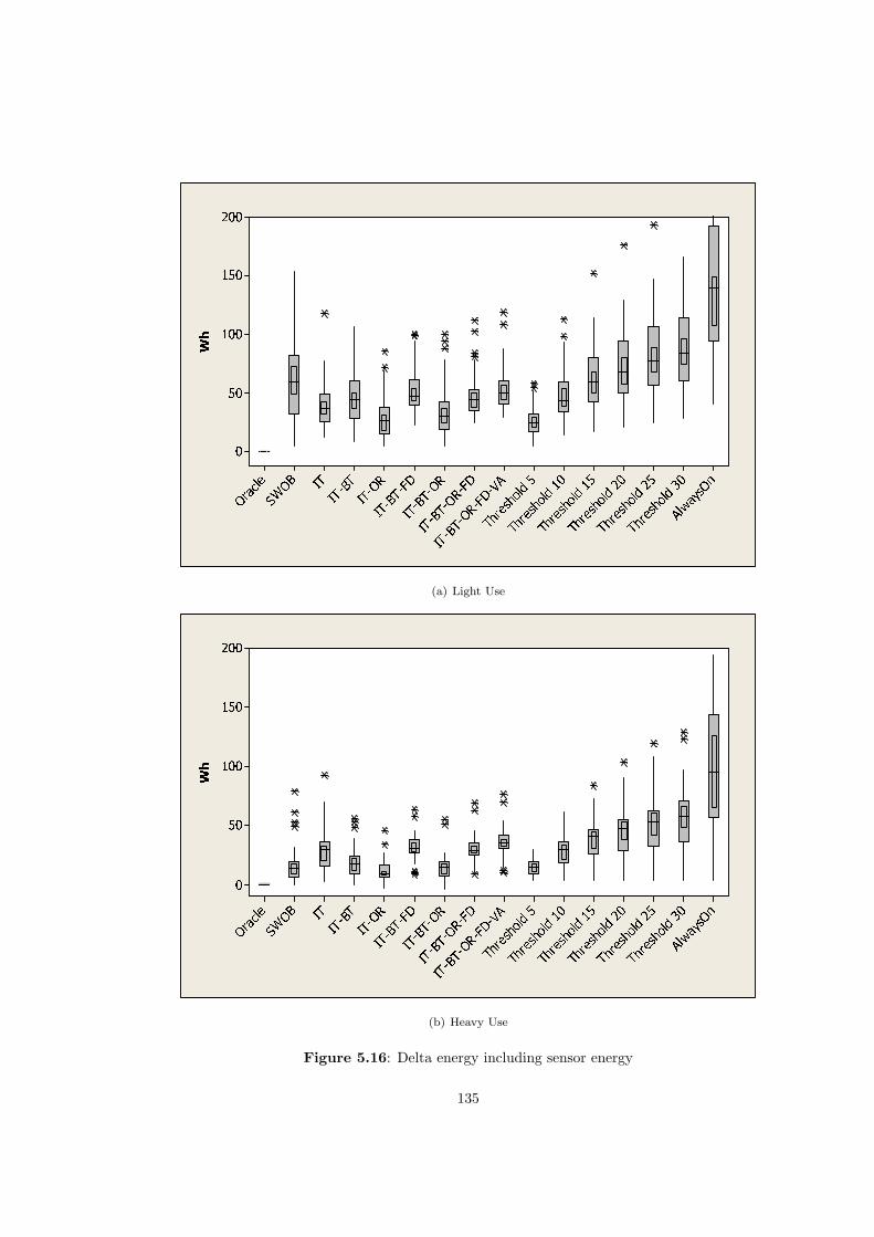
Wh
AlwaysOnThreshold 30Threshold 25Threshold 20Threshold 15Threshold 10Threshold 5IT-BT-OR-FD-VAIT-BT-OR-FDIT-BT-ORIT-BT-FDIT-ORIT-BTITSWOBOracle
200150100500(a) Light Use
Wh
AlwaysOnThreshold 30Threshold 25Threshold 20Threshold 15Threshold 10Threshold 5IT-BT-OR-FD-VAIT-BT-OR-FDIT-BT-ORIT-BT-FDIT-ORIT-BTITSWOBOracle
200150100500(b) Heavy Use
Figure 5.16: Delta energy including sensor energy
135

FPDs
AlwaysOnThreshold 30Threshold 25Threshold 20Threshold 15Threshold 10Threshold 5Threshold 4Threshold 3Threshold 2Threshold1IT-BT-OR-FD-VAIT-BT-OR-FDIT-BT-ORIT-BT-FDIT-ORIT-BTITSWOBOracle
302520151050(a) Light Use
FPD
AlwaysOnThreshold 30Threshold 25Threshold 20Threshold 15Threshold 10Threshold 5Threshold 4Threshold 3Threshold 2Threshold1IT-BT-OR-FD-VAIT-BT-OR-FDIT-BT-ORIT-BT-FDIT-ORIT-BTITSWOBOracle
302520151050(b) Heavy Use
Figure 5.17: False power downs
MPU
AlwaysOnThreshold 30Threshold 25Threshold 20Threshold 15Threshold 10Threshold 5Threshold 4Threshold 3Threshold 2Threshold1IT-BT-OR-FD-VAIT-BT-OR-FDIT-BT-ORIT-BT-FDIT-ORIT-BTITSWOBOracle
302520151050(a) Light Use
MPU
AlwaysOnThreshold 30Threshold 25Threshold 20Threshold 15Threshold 10Threshold 5Threshold 4Threshold 3Threshold 2Threshold1IT-BT-OR-FD-VAIT-BT-OR-FDIT-BT-ORIT-BT-FDIT-ORIT-BTITSWOBOracle
302520151050(b) Heavy Use
Figure 5.18: Manual power ups
136

Standby < Breakeven
AlwaysOnThreshold 30Threshold 25Threshold 20Threshold 15Threshold 10Threshold 5Threshold 4Threshold 3Threshold 2Threshold1IT-BT-OR-FD-VAIT-BT-OR-FDIT-BT-ORIT-BT-FDIT-ORIT-BTITSWOBOracle
20151050(a) Light Use
Standby < Breakeven
AlwaysOnThreshold 30Threshold 25Threshold 20Threshold 15Threshold 10Threshold 5Threshold 4Threshold 3Threshold 2Threshold1IT-BT-OR-FD-VAIT-BT-OR-FDIT-BT-ORIT-BT-FDIT-ORIT-BTITSWOBOracle
20151050(b) Heavy Use
Figure 5.19: Standby break-evens
range is significantly larger for the PC. The HeavyUse SWOB (median 4, range 0 to 10) compares
with the display values of median 1, range 0 to 6, where both the median and range are significantly
larger (see Figure 5.19). The BN policies for LightUse and HeavyUse have similar medians (LightUse
2 to 5.5, HeavyUse 1.0 to 4.0) but the range is slightly more for LightUse. Also, for the Threshold
policies the LightUse have slightly more standby break-even periods than for HeavyUse (LightUse -
Threshold1 14, Threshold5 4; HeavyUse - Threshold1 7, Threshold5 1).
To summarise, the overall pattern of results for power management of the PC are similar to that
of the display. For HeavyUse the SWOB policy is again the clear choice with both low delta energy
consumption 13Wh (5.7% from Oracle) and no FPDs and few MPUs. The fact that the break-even
time is longer means the policies achieve percentages closer to the Oracle policy. The number of
standby break-even periods would be a concern for the lifetime decay of this PC with median 4
standbys per day less than the 5 minute break-even period.
For LightUse the IT-BT-OR policy has one of the lowest delta energy consumptions 30Wh (12%
from Oracle) with the least FPDs and MPUs (FPDs median 0.5, MPUs median 3.75 per day). The
number of MPUs is significant as the resume time of 7 seconds will cause significant user annoyance.
The SWOB policy delta energy consumption for LightUse is 59Wh (22.1% from Oracle), which
appears to be the best overall policy due to it having no false power downs and very few manual
power ups (median 0).
137

5.6.6 DBN models for power management of the display
We experimented with dynamic Bayesian models to see if they could improve the predictive accuracy
of the policies, in particular, reduce the number of FPDs, MPUs and SBEs for the Bayesian policies.
The DBN for the display consists of six time slices with a 10 second interval between time slices. This
gives a prediction for not using that is 1 minute in the future.
Overall the performance of the DBN for power management of the display was very similar to
the standard BN. Figure 5.20 shows the delta energy consumption to be very similar to the standard
BN with the same policies performing the best. For LightUse IT-OR and IT-BT-OR are the best
energy-wise with medians 42Wh and 52Wh compared to 40Wh and 46Wh for the BN versions. For
HeavyUse the best DBN policies are IT-OR, IT-BT-OR and IT-BT with medians 16Wh, 25Wh,
26Wh compared with 21Wh, 21Wh, 25Wh for the BN versions.
The user-perceived performance figures are shown in Appendix A. The FPDs for the DBN policies
are in fact slightly worse than the BN policies with LightUse IT-BT-OR having median 0.75, range
0 to 5 and HeavyUse median 0.75, range 0 to 4. This compares to LightUse for the IT-BT-OR BN
having median 0.75, range 0 to 3 and HeavyUse median 0.5, range 0 to 2. The MPUs are similar to
the BN policies for the display, which is expected as the power-up policies for both are the same. The
SBE periods are also similar to the BN policies with LightUse medians from 1 to 2.5 and HeavyUse
from 1 to 1.5. The BN policies for the display have medians LightUse 1 to 2.25 and HeavyUse 0.25
to 2.0.
Overall there is no significant difference between the BN and DBN models for power management
of the display.
5.6.7 DBN models for power management of the PC
The DBN model for power management of the PC has 6 time slices with 50 second time intervals,
giving a prediction of not using that is 5 minutes into the future. Figure 5.21 shows the energy
consumption of the DBN policies to be significantly higher than the SWOB policy for both LightUse
and HeavyUse users. The user-perceived performance is an improvement on the BN polices (see
Figures in Appendix A).
The reason for the significant increase in energy consumption and improvement in user-perceived
performance is that the DBN policies take a long time for the not using probability to reach the
threshold and power down. Figure 5.22 shows the DBN IT-BT policy powering down 15 minutes
from the point of not using. From these results, it seems that the DBN models give no better
performance than the BN models.
138

Wh
AlwaysOnThreshold 30Threshold 25Threshold 20Threshold 15Threshold 10Threshold 5IT-BT-OR-FD-VAIT-BT-OR-FDIT-BT-ORIT-BT-FDIT-ORIT-BTITSWOBOracle
200150100500(a) Light Use
Wh
AlwaysOnThreshold 30Threshold 25Threshold 20Threshold 15Threshold 10Threshold 5IT-BT-OR-FD-VAIT-BT-OR-FDIT-BT-ORIT-BT-FDIT-ORIT-BTITSWOBOracle
200150100500(b) Heavy Use
Figure 5.20: DBN display delta energy including sensor energy
139

Wh
AlwaysOnThreshold 30Threshold 25Threshold 20Threshold 15Threshold 10Threshold 5IT-BT-OR-FD-VAIT-BT-OR-FDIT-BT-ORIT-BT-FDIT-ORIT-BTITSWOBOracle
200150100500(a) Light Use
Wh
AlwaysOnThreshold 30Threshold 25Threshold 20Threshold 15Threshold 10Threshold 5IT-BT-OR-FD-VAIT-BT-OR-FDIT-BT-ORIT-BT-FDIT-ORIT-BTITSWOBOracle
200150100500(b) Heavy Use
Figure 5.21: DBN PC delta energy including sensor energy
140

0
1
2
3
4
5
6
7
8
9
10
15:0
0:00
15:0
1:28
15:0
2:56
15:0
4:24
15:0
5:52
15:0
7:20
15:0
8:48
15:1
0:16
15:1
1:44
15:1
3:12
15:1
4:40
15:1
6:08
15:1
7:36
15:1
9:04
15:2
0:32
15:2
2:00
15:2
3:28
15:2
4:56
15:2
6:24
15:2
7:52
15:2
9:20
15:3
0:48
15:3
2:16
15:3
3:44
15:3
5:12
15:3
6:40
15:3
8:08
15:3
9:36
15:4
1:04
15:4
2:32
15:4
4:00
15:4
5:28
15:4
6:56
15:4
8:24
15:4
9:52
15:5
1:20
15:5
2:48
15:5
4:16
15:5
5:44
15:5
7:12
15:5
8:40
Figure 5.22: Example DBN policy trace
5.7 Evaluation of the affect of monitoring on users
It was necessary to evaluate if the user’s behaviour was affected by the monitoring of the using and
not using periods during the trial. We assumed that if there was an affect it would be that the
users would make more frequent inputs due to the message box popping up. For example, when
the user was prompted to confirm they were using the PC, they would change from what they were
doing to use the mouse or keyboard and hence create a short idle period of less than 1 minute. If
they just tipped the mouse to signify they were using the PC and continue their activity (for example
reading from the display), the measured idle period is longer. This is because the short mouse input is
removed from the measured trace during the data processing. So, if the monitoring affected the user’s
behaviour there would be significantly more short idle periods of duration 30 seconds to 1 minute.
To evaluate this we compared the frequency of idle periods in 1 minute bins (from 0 to < 1 minutes
to >= 30 minutes) for the trial week and 5 normal weeks when just the idle periods were recorded.
The measured trace for the trial week was processed to leave just the idle periods, so it could be
compared with the traces of the 5 normal weeks. The analysis was done for a random sample of 8 of
the users.
Figure 5.23 shows graphs of idle period frequencies for 6 of these users for the trial week and the
5 normal weeks. The trial week is the thicker line with the circle markers. The graphs show that
the idle period frequencies for the trial week do not vary significantly outside of the normal weekly
variability for each user. This suggests that the monitoring of the trial week did not have a significant
effect on the users’ frequency of input.
141

0
50
100
150
200
250
300
1 2 3 4 5 6 7 8 9 10 11 12 13 14 15 16 17 18 19 20 21 22 23 24 25 26 27 28 29 30 31
idle period
frequ
ency
0
50
100
150
200
250
300
1 2 3 4 5 6 7 8 9 10 11 12 13 14 15 16 17 18 19 20 21 22 23 24 25 26 27 28 29 30 31
idle periodfre
quen
cy
0
50
100
150
200
250
300
1 2 3 4 5 6 7 8 9 10 11 12 13 14 15 16 17 18 19 20 21 22 23 24 25 26 27 28 29 30 31
idle period
frequ
ency
0
50
100
150
200
250
300
1 2 3 4 5 6 7 8 9 10 11 12 13 14 15 16 17 18 19 20 21 22 23 24 25 26 27 28 29 30 31
idle period
frequ
ency
0
50
100
150
200
250
300
1 2 3 4 5 6 7 8 9 10 11 12 13 14 15 16 17 18 19 20 21 22 23 24 25 26 27 28 29 30 31
idle period
frequ
ency
0
50
100
150
200
250
300
1 2 3 4 5 6 7 8 9 10 11 12 13 14 15 16 17 18 19 20 21 22 23 24 25 26 27 28 29 30 31
idle period
frequ
ency
Figure 5.23: Idle traces for 6 of the users
142

0
0.1
0.2
0.3
0.4
0.5
0.6
0.7
0.8
0.9
1
0 1 2 3
Bluetooth count
prob
abili
ty
(a) Light Use
0
0.1
0.2
0.3
0.4
0.5
0.6
0.7
0.8
0.9
1
0 1 2 3
Bluetooth count
prob
abili
ty
(b) HeavyUse
Figure 5.24: Bluetooth parameters given the user is not using
5.8 Evaluation of BNs for device power management
Bayesian networks were used to implement the CAPM power-down policies. The supervised param-
eter learning captured the probability of each sensor value inferring not using and the network
combined these to give an overall not using probability. Figure 5.24 shows the learned BT param-
eters given the user is not using, for a LightUse and HeavyUse user. For the LightUse user, the
presence of the BT tag has a greater probability of not using than for the HeavyUse user. Therefore
for a LightUse user in the vicinity of the PC, the probability of not using will be reached more
quickly as their presence is not a good indication of them using the PC.
However, there were some issues with the BN models. A rule had to be put into the model (the
IdleTimeZero node) to infer using if the idle time was less than 1 minute. This avoided a significant
number of false power downs as the BN models could infer not using too quickly. This would occur
when the learned sensor parameters were stronger than the learned IdleTime parameter for 0 to 1
minute idle time and hence were too quick to predict a high probability of not using.
The parameter learning for sensor values can be irregular if some of the sensor values are only
lightly sampled. The parameter learning algorithm needs sufficient samples of a parameter value
to give an accurate probability estimate for that value. This was in particular a problem for the
IdleTime sensor where in most cases the probability of not using fluctuated when the idle time
became greater than about 9 minutes, as there were few samples for idle times greater than this. One
possible solution discussed in Section 4.1.1 is to apply a smoothing function to the idle time CPTs
to reduce the fluctuation in the not using probability. Another possible solution could be to use a
more conservative fixed parameter for the IdleTime to avoid the false power downs suffered by the
143

0
0.1
0.2
0.3
0.4
0.5
0.6
0.7
0.8
0.9
1
0 1 2 3
Bluetooth count
prob
abili
ty
(a) Bluetooth given Not Using
0
0.1
0.2
0.3
0.4
0.5
0.6
0.7
0.8
0.9
1
0 1 2 3
Bluetooth count
prob
abili
ty
(b) Bluetooth given Using
Figure 5.25: Variance in BT parameters for the 5 training days
BN policies.
The learning of the power-down policy parameters was based on supervised data as we fully
measured when the user was using and not using the PC using the pop-up message box. It would
not be practical to do this in a deployment CAPM situation as it causes user annoyance to ask the
user if they are using the PC or not after every minute of idleness. So, a semi-supervised method of
learning the parameters would have to be developed. This method would only detect the user not
using the PC when it is powered down and using the PC when the idle time is close to zero, say
less than ten seconds. The other intervening cases would not be known.
Also, by looking at the parameter learning for each of the cross-fold training days, some of the
LightUse users show significant variability in the parameter learning depending on which day was
chosen (see Figure 5.25). This can significantly affect the outcome performance of the policies. Figure
5.26 shows the corresponding variability in policy energy consumption depending on the day it was
trained on. The IT, IT-BT and IT-BT-FD policies have large variability for this LightUse user. For
these variable use users, parameter learning over a longer period will produce an average parameter
but the user’s usage will vary significantly from this average.
Finally, the learning of the power-up policies was not successful as the learned about to use
probabilities were very variable across the users. For example, with the simple IT-BT model, the
probability of about to use when the BT tag was detected varied from around 40% to 80% for each
of the users. A simple rule-based policy was more appropriate where the device always powered up
when the BT tag was detected.
144

Wh
IT-BT-OR-FD-VAIT-BT-OR-FDIT-BT-ORIT-BT-FDIT-ORIT-BTIT
1300125012001150110010501000Figure 5.26: Variance in energy consumption per training day
5.9 Summary
The results show clearly that for HeavyUse (<= 15% not using when in the vicinity) users of the
display and PC, the SWOB policy does as well as the BN policies energy-wise, 22Wh (9%) from
Oracle per day for the display and 13Wh (6%) from Oracle per day for the PC. Furthermore, the
user-perceived performance of the SWOB policy is better with no FPDs and median 0, range 0 to 2
MPUs. The BN policies incur a number of FPDs (median 0.25 to 0.75, range 0 to 5) and on average
one MPU per day. The Threshold 5 policy performs similarly well energy-wise and has median
0 FPDs, however has significant MPUs (median 5 per day). Therefore, we can conclude that for
HeavyUse users the SWOB policy is the most appropriate for power management of the display and
PC.
For LightUse (> 15% not using when in the vicinity) users there is potential to do better than
the SWOB policy. On average the potential extra energy that can be saved beyond the simple SWOB
policy for LightUse users of the display is 78Wh (31%) from Oracle per day and for the PC is 59Wh
(22%) from Oracle per day. However, the results show that it is difficult to do significantly better
energy-wise than the SWOB policy without incurring performance penalties of false power downs and
manual power ups.
For LightUse users of the display the best BN policy is IT-BT-OR with energy consumption of
46Wh (19%) from Oracle and from 0 to 3 FPDs (median 0.75) per day and on average 4.75 MPUs
145

per day. The Threshold 5 policy does similarly energy-wise (46Wh) and has less FPDs (median 0,
range 0 to 2) but more MPUs (median 8). We believe that with further tuning of the BN model, the
FPDs could be improved for IT-BT-OR. Therefore we recommend the IT-BT-OR policy as the most
suitable policy for power management of LightUse usage of the display.
For LightUse users of the PC, the best BN policy is again IT-BT-OR with energy consumption
of 30Wh (12%) from Oracle and 0 to 2 FPDs (median 0.5) per day and on average 3.75 MPUs.
The Threshold 5 policy does similarly energy-wise (24Wh), has fewer FPDs (median 0, range 0 to
2) but again more MPUs (median 8). While the performance of the IT-BT-OR policy might be
acceptable for power management of the display, as the resume time is quick, we believe it would
be unacceptable for the PC and hence the SWOB policy should also be recommended for power
management of LightUse usage of the PC.
In all cases the face detection sensor consumes significantly more energy than the object range
detection sensor and does not provide significantly better information. The voice activity sensor
information does not improve the IT-BT-OR-FD policy at all as the quality of its information for
determining not using is very weak.
For the recommended policies for power management of the display (LightUse - IT-BT-OR;
HeavyUse - SWOB) the SBE periods are relatively low (median 2, range 0 to 5; median 1, range
0 to 5) per day. However, for the PC the recommended SWOB policy incurs a significant number of
SBEs (LightUse - median 2, range 0 to 11; HeavyUse - median 4, range 0 to 10). This would be a
concern for power management of devices that incur a significant lifetime decay from switching on
and off frequently. Possibly the inclusion of time of day information may help to reduce the number
of short standby periods, or failing this knowledge of the user’s distributed location may be needed
to predict longer break-even periods. For example, if the user has gone to the bathroom they may be
back soon but if they have left the building it is likely they will be back later.
The DBN policies did not perform better than the BN policies and in the case of the PC performed
significantly worse energy wise due to the long delay before powering down.
It is possible that more tailor made rule-based policies could do better than the BN policies,
achieving similar energy consumption but reducing the number of FPDs. However, we believe the
number of manual power ups will remain similar due to the difficulty of automatically powering up
in time when the user is in the vicinity. Therefore, the conclusions would still remain the same for
the power management policies. For HeavyUse users, user presence (BT tag) is sufficient, whereas for
LightUse users, user presence and near presence (OR detection) do better for the display, but incur
too many MPUs for the PC which has a long resume time.
146

Chapter 6
Conclusions
This thesis began by outlining the motivation for device power management in buildings. There is
a pressing need to reduce overall energy consumption, however, in spite of this there has been a
steady rise in the energy consumed by electrical devices in buildings. Pervasive computing could
further exacerbate the building energy problem, but on the other hand it could provide a solution by
enabling more intelligent context-aware power management of devices.
Chapter 2 reviewed the current state of the art in dynamic power management and context-aware
power management. The review concluded that current dynamic power management techniques are
primarily focused on management of mobile, battery-powered devices and are not suitable for power
management of stationary devices, which have longer break-even and resume times. Furthermore, it
is necessary to obtain context from the user-level (e.g., user location) for effective power management
of stationary devices. There have been several research projects in this area of CAPM, which have
focused on developing techniques for inferring context from sensors. However, there has been no
detailed study into what are the potential energy savings of CAPM and what granularity of context
is appropriate.
6.1 Contribution
The initial experimental trial explored the use of location as a key piece of context for power man-
agement of desktop PCs in an office environment. The resulting SWOB policy powers down the PC
when the user’s presence (Bluetooth phone) is not detected and powers up again when the phone
is detected again. The trial demonstrated that user behaviour is the key factor to the SWOB pol-
icy’s performance. For heavy users, the SWOB policy performs well both in terms of energy and
147

user-perceived performance and for light users it performs badly energy-wise but maintains good
user-perceived performance.
A large user study was carried out to evaluate whether additional, finer-grained context could
do better than the SWOB policy and at what extra cost. The sensors explored were idle time (IT),
Bluetooth presence (BT), face detection (FD), object range detection (OR), and voice activity (VA).
A Bayesian network was used to combine the multi-modal data to infer the contexts not using and
about to use.
The user study revealed the potential extra energy that could be saved beyond that of the SWOB
policy was relatively small for heavy users (6-9% from Oracle). The BN policies with additional
sensors did no better energy-wise and had worse user-perceived performance (median 1 MPU per
day) because these policies power down when the user is still in the vicinity of the device. Therefore,
the SWOB policy is recommended for heavy users of displays and PCs. For light users the SWOB
policy does not perform as well energy-wise (22-31% from Oracle) and the best performing CAPM
policy is IT-BT-OR (12-19% from Oracle). However, there are a significant number of manual power
ups (median 4 to 5 per day) for IT-BT-OR. Therefore, we believe this policy would only be suitable
for power management of displays, which have a short resume time.
The energy consumption of the face detection and voice activity sensors was found to be significant
(FD 20.2Wh, VA 6.4Wh median per day) compared to the potential extra energy that can be saved
for light users (PC 59Wh and display 78Wh median per day). The large energy consumption is due
to the significant amount of CPU processing of the video and audio data. Furthermore, we found
the voice activity sensor did not provide a good cue of the contexts not using and about to use.
Although, the face detection sensor provided valuable information, the energy cost of the sensor
resulted in it performing worse overall than the coarser-grained object-range sensor.
The technique of Bayesian networks did not perform as well as we expected with the BN policies
having a significant number of false power downs, more than the Threshold 5 policy. We believe
that some hand-crafting of the BN parameters would be needed to reduce the number of FPDs to
an acceptable level. Furthermore, the dynamic Bayesian network was not an improvement over the
standard BN. Given the IT-BT-OR policy has relatively few sensors, it is possible that a simple
rule-based policy could do as well, if not better than the BN technique.
148

6.2 Future work
This thesis focused on the off-line evaluation of the BN policies. These policies were trained with
supervised data gathered from the measurement of the users’ usage. Currently the runtime CAPM
framework does not incorporate on-line learning of the CPTs. In the on-line case it is not practical to
fully measure when the user is using and not using the device, as this would cause significant user
annoyance. Therefore, there is a need to develop a semi-supervised approach to learning of the CPTs,
where it is possible to learn the CPTs based on a partial set of observed using and not using cases.
Furthermore, given the results from the evaluation, it would also be necessary to explore techniques
to avoid false power downs occurring.
Another finding from the evaluation is that user behaviour could vary significantly. For some of
the light users, their behaviour changed from day to day, with some days being light use and others
more heavy use. Therefore, another issue to deal with is learning for users with variable behaviour.
Finally, the requirements of distant prediction and distributed sensing were not implemented
in the CAPM framework. These requirements could be addressed by inclusion of CAPM into the
sentient object model. This would enable inclusion of data from distributed sensors, for example,
the location of a user in other parts of the building. This could enable the prediction of longer idle
periods necessary to reduce the number of standbys that are less than the break-even time for devices
with long break-even times (5 minutes and greater). In addition, mobility prediction could be used
for distant prediction to offset delays in sensor response and long device resume times.
149

Appendix A
Additional Evaluation Figures
150

FPD
AlwaysOnThreshold 30Threshold 25Threshold 20Threshold 15Threshold 10Threshold 5Threshold 4Threshold 3Threshold 2Threshold1IT-BT-OR-FD-VAIT-BT-OR-FDIT-BT-ORIT-BT-FDIT-ORIT-BTITSWOBOracle
302520151050(a) Light Use
FPD
AlwaysOnThreshold 30Threshold 25Threshold 20Threshold 15Threshold 10Threshold 5Threshold 4Threshold 3Threshold 2Threshold1IT-BT-OR-FD-VAIT-BT-OR-FDIT-BT-ORIT-BT-FDIT-ORIT-BTITSWOBOracle
302520151050(b) Heavy Use
Figure A.1: DBN display false power downs
MPU
AlwaysOnThreshold 30Threshold 25Threshold 20Threshold 15Threshold 10Threshold 5Threshold 4Threshold 3Threshold 2Threshold1IT-BT-OR-FD-VAIT-BT-OR-FDIT-BT-ORIT-BT-FDIT-ORIT-BTITSWOBOracle
302520151050(a) Light Use
MPU
AlwaysOnThreshold 30Threshold 25Threshold 20Threshold 15Threshold 10Threshold 5Threshold 4Threshold 3Threshold 2Threshold1IT-BT-OR-FD-VAIT-BT-OR-FDIT-BT-ORIT-BT-FDIT-ORIT-BTITSWOBOracle
302520151050(b) Heavy Use
Figure A.2: DBN display manual power ups
151

Standby < Breakeven
AlwaysOnThreshold 30Threshold 25Threshold 20Threshold 15Threshold 10Threshold 5Threshold 4Threshold 3Threshold 2Threshold1IT-BT-OR-FD-VAIT-BT-OR-FDIT-BT-ORIT-BT-FDIT-ORIT-BTITSWOBOracle
20151050(a) Light Use
Standby < Breakeven
AlwaysOnThreshold 30Threshold 25Threshold 20Threshold 15Threshold 10Threshold 5Threshold 4Threshold 3Threshold 2Threshold1IT-BT-OR-FD-VAIT-BT-OR-FDIT-BT-ORIT-BT-FDIT-ORIT-BTITSWOBOracle
20151050(b) Heavy Use
Figure A.3: DBN display standby break-evens
FPD
AlwaysOnThreshold 30Threshold 25Threshold 20Threshold 15Threshold 10Threshold 5Threshold 4Threshold 3Threshold 2Threshold1IT-BT-OR-FD-VAIT-BT-OR-FDIT-BT-ORIT-BT-FDIT-ORIT-BTITSWOBOracle
302520151050(a) Light Use
FPD
AlwaysOnThreshold 30Threshold 25Threshold 20Threshold 15Threshold 10Threshold 5Threshold 4Threshold 3Threshold 2Threshold1IT-BT-OR-FD-VAIT-BT-OR-FDIT-BT-ORIT-BT-FDIT-ORIT-BTITSWOBOracle
302520151050(b) Heavy Use
Figure A.4: DBN PC false power downs
152

MPU
AlwaysOnThreshold 30Threshold 25Threshold 20Threshold 15Threshold 10Threshold 5Threshold 4Threshold 3Threshold 2Threshold1IT-BT-OR-FD-VAIT-BT-OR-FDIT-BT-ORIT-BT-FDIT-ORIT-BTITSWOBOracle
302520151050(a) Light Use
MPU
AlwaysOnThreshold 30Threshold 25Threshold 20Threshold 15Threshold 10Threshold 5Threshold 4Threshold 3Threshold 2Threshold1IT-BT-OR-FD-VAIT-BT-OR-FDIT-BT-ORIT-BT-FDIT-ORIT-BTITSWOBOracle
302520151050(b) Heavy Use
Figure A.5: DBN PC manual power ups
Standby < Breakeven
AlwaysOnThreshold 30Threshold 25Threshold 20Threshold 15Threshold 10Threshold 5Threshold 4Threshold 3Threshold 2Threshold1IT-BT-OR-FD-VAIT-BT-OR-FDIT-BT-ORIT-BT-FDIT-ORIT-BTITSWOBOracle
20151050(a) Light Use
Standby < Breakeven
AlwaysOnThreshold 30Threshold 25Threshold 20Threshold 15Threshold 10Threshold 5Threshold 4Threshold 3Threshold 2Threshold1IT-BT-OR-FD-VAIT-BT-OR-FDIT-BT-ORIT-BT-FDIT-ORIT-BTITSWOBOracle
20151050(b) Heavy Use
Figure A.6: DBN PC standby break-evens
153

Bibliography
[1] Kolmogorov A. Grundbegriffe der warhscheinlichkeitsrechnung.
Springer Verlag, 1933.
[2] Luca Benini, Alessandro Bogliolo, and Giovanni De Micheli. A survey
of design techniques for system-level dynamic power management. IEEE
Transactions on Very Large Scale Integration (VLSI) Systems,
8(3):299-316, June 2000.
[3] Gregory Biegel. A Programming Model for Mobile, Context-Aware
Applications. PhD thesis, University of Dublin, Trinity College,
2004.
[4] Gregory Biegel and Vinny Cahill. A framework for developing mobile,
context-aware applications. In Proceedings of the 2nd IEEE
International Conference on Pervasive Computing and Communications
(PerCom 2004), pages 361-365. IEEE Computer Society, March 2004.
[5] BlueLon. Bodytag bt-002. http://www.bluelon.com/.
[6] Gary Bradski, Adrian Kaehler, and Vadim Pisarevsky. Learning-based
computer vision with intel’s open source computer vision library.
Compute-Intensive, Highly Parallel Applications and Uses, 09(01),
2005.
[7] Matthew Brand and Vera Kettnaker. Discovery and segmentation of
activities in video. IEEE Trans. Pattern Anal. Mach. Intell.,
22(8):844-851, 2000.
[8] Jennifer Bray and Charles F Sturman. Bluetooth Connect Without
Cables. Prentice Hall, 2001.
154

[9] B.G. Buchanan and E.H. Shortliffe. Rule-Based Expert Systems: The
MYCIN Experiments of the Stanford Heuristic Programming Project.
Addison-Wesley, 1984.
[10] Victor Callaghan. The intelligent dormitory homepage.
http://cswww.essex.ac.uk/Research/iieg/idorm.htm.
[11] Suan Khai Chong, Shonali Krishnaswamy, and Seng Wai Loke. A
context-aware approach to conserving energy in wireless sensor
networks. In First International Workshop on Sensor Networks and
Systems for Pervasive Computing, 2005.
[12] Michael H. Coen. Design principles for intelligent environments. In
AAAI ’98/IAAI ’98: Proceedings of the fifteenth national/tenth
conference on Artificial intelligence/Innovative applications of
artificial intelligence, pages 547-554, Menlo Park, CA, USA, 1998.
American Association for Artificial Intelligence.
[13] European Comission. Towards a european strategy for the security of
energy supply, 2000.
http://europa.eu.int/comm/energy_transport/en/lpi_lv_en1.html.
[14] European Comission. Towards a european strategy for the security of
energy supply (technical document), 2000.
http://europa.eu.int/comm/energy_transport/en/lpi_lv_en1.html.
[15] European Comission. 5e in universities, 2003.
http://www.copernicus-campus.org/sites/5EinUniversities.html.
[16] Diane J. Cook. Mavhome smart home project. http://mavhome.uta.edu/.
[17] Anind K. Dey and Gregory D. Abowd. Towards a better understanding of
context and context-awareness. Technical Report GIT-GVU-99-22,
Georgia Institute of Technology, 1999.
[18] T. Dietterich. Statistical tests for comparing supervised
classification learning algorithms. Technical report, Department of
Computer Science, Oregon State University, 1996.
[19] Faiyaz Doctor, Hani Hagras, and Victor Callaghan. An adaptive fuzzy
learning mechanism for intelligent. agents in ubiquitous computing
155

environments. In 6th Biannual World Automation Conference, pages
101-106. TSI Press Series, 2004.
[20] Fred Douglis, P. Krishnan, and Brian Marsh. Thwarting the
power-hungry disk. In USENIX Winter, pages 292-306, 1994.
[21] Robot Electronics. Srf08 ultra sonic range finder technical
specification.
http://www.robot-electronics.co.uk/htm/srf08tech.shtml.
[22] Carla Ellis. The case for higher-level power management. In The
Seventh Workshop on Hot Topics in Operating Systems, Rio Rico,
Arizona, pages 162-167, March 28 - 30 1999.
[23] Jason Flinn, Eyal de Lara, Mahadev Satyanarayanan, Dan S. Wallach,
and Willy Zwaenepoel. Reducing the energy usage of office
applications. In Middleware 2001: Proceedings of the IFIP/ACM
International Conference on Distributed Systems Platforms Heidelberg,
pages 252-272, London, UK, 2001. Springer-Verlag.
[24] Jason Flinn and M. Satyanarayanan. Energy-aware adaptation for
mobile applications. In Symposium on Operating Systems Principles,
pages 48-63, 1999.
[25] Oliver Gassmann and Hans Meixner. Sensors in Intelligent Buildings.
Wiley, 2001.
[26] Colin Harris and Vinny Cahill. Exploiting user behaviour for
context-aware power management. In International Conference On
Wireless and Mobile Computing, Networking and Communications, pages
122-130. IEEE, August 2005.
[27] Edwin O. Heierman and Diane J. Cook. Improving home automation by
discovering regularly occurring device usage patterns. In ICDM ’03:
Proceedings of the Third IEEE International Conference on Data
Mining, page 537, Washington, DC, USA, 2003. IEEE Computer Society.
[28] Hewlett-Packard, Intel, Microsoft, Phoenix, and Toshiba. Advanced
configuration and power interface. http://www.acpi.info/.
[29] Intel. Integrated performance primitives.
156

http://www.intel.com/cd/software/products/asmo-
na/eng/perflib/ipp/index.htm.
[30] Intel. Opencv. http://sourceforge.net/projects/opencvlibrary/.
[31] Ravi Jain and John Wullert, II. Challenges: environmental design
for pervasive computing systems. In Proceedings of the 8th Annual
International Conference on Mobile Computing and Networking, pages
263-270. ACM Press, 2002.
[32] Anna R. Karlin, Mark S. Manasse, Lyle A. McGeoch, and Susan S.
Owicki. Competitive randomized algorithms for nonuniform problems.
In Algorithmica, volume 11, pages 542-571, 1994.
[33] Kaoru Kawamoto, Jonathan G. Koomey, Bruce Nordman, Richard Brown,
Mary Ann Piette, and Alan K. Meier. Electricity used by office
equipment and network equipment in the u.s. In Proceedings of the
2000 ACEEE Summer Study on Energy Efficiency in Buildings. ACEEE,
2000.
[34] Jerzy Kolinsky, Ram Chary, Andrew Henroid, and Barry Press. Building
the power-efficient PC. Intel Press, 2001.
[35] Kevin Korb and Ann Nicholson. Bayesian Artificial Intelligence.
Chapman and Hall/CRC Press UK, 2004.
[36] Robin Kravets and P. Krishnan. Application-driven power management
for mobile communication. Wireless Networks, 6(4):263-277, 2000.
[37] Y. Lu, T. Simunic, and G. De Micheli. Software controlled power
management. In IEEE Hardware/Software Co-Design Workshop, pages
157-161, May 1999.
[38] Yung-Hsiang Lu, Luca Benini, and Giovanni De Micheli.
Operating-system directed power reduction. In International
Symposium on Low Power Electronics and Design, pages 37-42. Stanford
University, July 2000.
[39] Yung-Hsiang Lu, Eui-Young Chung, Tajana Simunic, Luca Benini, and
Giovanni De Micheli. Quantitative comparison of power management
algorithms. In Design Automation and Test in Europe, pages 20-26.
Stanford University, March 2000.
157

[40] Ren C. Luo and Michael G. Kay. Multisensor integration and fusion in
intelligent systems. In Transactions on Systems, Man, and
Cybernetics, volume 19, pages 901-931. IEEE, September 1989.
[41] Anant Madabhushi and J. K. Aggarwal. A bayesian approach to human
activity recognition. In VS ’99: Proceedings of the Second IEEE
Workshop on Visual Surveillance, page 25, Washington, DC, USA, 1999.
IEEE Computer Society.
[42] Michael Mozer. Adaptive house project.
http://www.cs.colorado.edu/ mozer/nnh/.
[43] Michael Mozer. Smart environments: Technologies, protocols, and
applications, chapter 12, pages 273-294. J. Wiley and Sons, November
2004.
[44] Kevin Murphy. Software packages for graphical models.
http://www.cs.ubc.ca/ murphyk/Bayes/bnsoft.html.
[45] United Nations. Kyoto protocol to the united nations framework
convention on climate change.
http://unfccc.int/essential_background/kyoto_protocol/items/1678.php.
[46] Richard E. Neapolitan. Learning Bayesian Networks. Prentice Hall,
April 2003.
[47] The Chartered Institution of Building Services Engineers. Energy
consumption guide 19, 2000.
[48] N. Oliver, E. Horvitz, and A. Garg. Layered representations for
human activity recognition. In Fourth IEEE Int. Conf. on Multimodal
Interfaces, pages 3-8, 2002.
[49] Nuria Oliver and Eric Horvitz. S-seer: Selective perception in a
multimodal office activity recognition system. In MLMI, pages
122-135, 2004.
[50] Nuria Oliver and Eric Horvitz. A comparison of hmms and dynamic
bayesian networks for recognizing office activities. In User
Modeling, pages 199-209, 2005.
[51] G. A. Paleologo, L. Benini, A. Bogliolo, and G. De Micheli. Policy
optimization for dynamic power management. In Proceedings of the
158

35th annual conference on Design automation conference, pages
182-187. ACM Press, 1998.
[52] Matthai Philipose, Kenneth P. Fishkin, Mike Perkowitz, Donald J
Patterson Dirk Hahnel, Dieter Fox, and Henry Kautz. Inferring
Activities from Interactions with Objects. In IEEE Pervasive
Computing: Mobile and Ubiquitous Systems, volume 3, pages 50-57.
IEEE, 2004.
[53] Lawrence Rabiner and Biing-Hwang Juang. Fundamentals of speech
recognition. Prentice-Hall, Inc., Upper Saddle River, NJ, USA, 1993.
[54] J. Rissanen. Modelling by shortest data description. Automatica,
14:465-471, 1978.
[55] Abhishek Roy, Soumya K. Das Bhaumik, Amiya Bhattacharya, Kalyan Basu,
Diane J. Cook, and Sajal K. Das. Location aware resource management
in smart homes. In IEEE International Conference on Pervasive
Computing and Communications, page 481. IEEE, March 2003.
[56] Stuart Russell and Peter Norvig. Artificial Intelligence: A Modern
Approach. Prentice Hall, second edition, 2003.
[57] Jerome H. Saltzer, David P. Reed, and David D. Clark. End-to-end
arguments in system design. ACM Transactions on Computer Systems,
2(4):277-288, November 1984.
[58] M. Satyanarayanan. Pervasive computing: Vision and challenges. IEEE
Personal Communications, pages 10-17, August 2001.
[59] Paul A. Shirley. An introduction to ultrasonic sensing. The Journal
of Machine Perception, 6(11), 1989.
[60] Tajana Simunic, Luca Benini, Peter W. Glynn, and Giovanni De Micheli.
Dynamic power management for portable systems. In Mobile Computing
and Networking, pages 11-19, 2000.
[61] D. J. Spiegelhalter and S. L. Lauritzen. Sequential updating of
conditional probabilities on directed graphical structures.
Networks, 20:579-605, 1990.
[62] Carl Steinbach. A reinforcement-learning approach to power
159

management. Technical report, Artificial Intelligence Laboratory,
MIT, 2002.
[63] Eino Tetri. Profitability of switching off fluorescent lamps:
Take-a-break. In RIGHT LIGHT 4, volume 1, pages 113-116, 1997.
[64] P. Viola and M. Jones. Rapid object detection using a boosted
cascade of simple features. In CVPR, 2001.
[65] von Mises R. Probability, Statistics, and Truth. Allen and Unwin,
1957.
[66] Mark Weiser. The computer for the 21st century. Scientific American,
265(3):94-104, September 1991.
[67] Mark Weiser, Brent Welch, Alan J. Demers, and Scott Shenker.
Scheduling for reduced CPU energy. In Operating Systems Design and
Implementation, pages 13-23, 1994.
[68] Robert Yarham. Natural Ventilation in Non-Domestic Buildings. CIBSE,
1997.
[69] H. Zeng, C. Ellis, A. Lebeck, and A. Vahdat. Currentcy: Unifying
policies for resource management. Technical Report CS-2002-09, Duke
University, Computer Science, May 2002.
[70] Heng Zeng, Xiaobo Fan, Carla Ellis, Alvin Lebeck, and Amin Vahdat.
ECOSystem: Managing energy as a first class operating system
resource. In Tenth International Conference on Architectural Support
for Programming Languages and Operating Systems (ASPLOS X), October
2002.
160