continuous probability distributionscathy/math3339/lecture/lect7...continuous probability...
TRANSCRIPT

Continuous Probability DistributionsSections 5.1 - 5.4
Cathy Poliak, [email protected]
Office in 11c Flemming
Department of MathematicsUniversity of Houston
Lecture 7 - 3339
Cathy Poliak, Ph.D. [email protected] Office in 11c Flemming (Department of Mathematics University of Houston )Sections 5.1 - 5.4 Lecture 7 - 3339 1 / 53

You Try Questions
For each random variable, determine if it is:
a. Discrete b. Continuous
2. The number of cars passing a busy intersection between 4:30 PMand 6:30 PM.
3. The weight of a fire fighter.
4. The amount of soda in a can of Pepsi.
Cathy Poliak, Ph.D. [email protected] Office in 11c Flemming (Department of Mathematics University of Houston )Sections 5.1 - 5.4 Lecture 7 - 3339 2 / 53

Types of Random Variables
A random variable that may assume either a finite number ofvalues or an infinite sequence of values such as 0,1, . . . is referredto as a discrete random variable.
A random variable that may assume any numerical value in aninterval or collection of intervals is called a continuous randomvariable.
Cathy Poliak, Ph.D. [email protected] Office in 11c Flemming (Department of Mathematics University of Houston )Sections 5.1 - 5.4 Lecture 7 - 3339 3 / 53

Example
Suppose we want to determine the probability of waiting for anelevator where the longest waiting time is 5 minutes.
What type of variable do we have?
Suppose we take a sample of 10, 50, 1000, and 10,000 people tosee how long they wait for the elevator. The following arehistograms for the waiting times of each sample.
Cathy Poliak, Ph.D. [email protected] Office in 11c Flemming (Department of Mathematics University of Houston )Sections 5.1 - 5.4 Lecture 7 - 3339 4 / 53

Sample of 10 People Waiting for the Elevator
Histogram of a Sample of 10
Minutes
Den
sity
0 1 2 3 4 5
0.0
0.1
0.2
0.3
0.4
Cathy Poliak, Ph.D. [email protected] Office in 11c Flemming (Department of Mathematics University of Houston )Sections 5.1 - 5.4 Lecture 7 - 3339 5 / 53

Sample of 50 People Waiting for the Elevator
Histogram of a Sample of 50
Minutes
Den
sity
0 1 2 3 4 5
0.00
0.05
0.10
0.15
0.20
0.25
Cathy Poliak, Ph.D. [email protected] Office in 11c Flemming (Department of Mathematics University of Houston )Sections 5.1 - 5.4 Lecture 7 - 3339 6 / 53
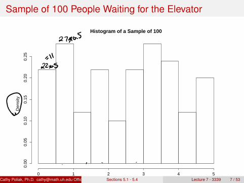
Sample of 100 People Waiting for the Elevator
Histogram of a Sample of 100
Minutes
Den
sity
0 1 2 3 4 5
0.00
0.05
0.10
0.15
0.20
0.25
Cathy Poliak, Ph.D. [email protected] Office in 11c Flemming (Department of Mathematics University of Houston )Sections 5.1 - 5.4 Lecture 7 - 3339 7 / 53

Sample of 1000 People Waiting for the Elevator
Histogram of a Sample of 1000
Minutes
Den
sity
0 1 2 3 4 5
0.00
0.05
0.10
0.15
0.20
0.25
Cathy Poliak, Ph.D. [email protected] Office in 11c Flemming (Department of Mathematics University of Houston )Sections 5.1 - 5.4 Lecture 7 - 3339 8 / 53

Sample of 10,000 People Waiting for the Elevator
Histogram of a Sample of 10,000
Minutes
Den
sity
0 1 2 3 4 5
0.00
0.05
0.10
0.15
0.20
Cathy Poliak, Ph.D. [email protected] Office in 11c Flemming (Department of Mathematics University of Houston )Sections 5.1 - 5.4 Lecture 7 - 3339 9 / 53


Probability distributions
A probability distribution for random variables describes howprobabilities are distributed over the values of the random variable.
For a discrete random variable X , the probability distribution isdefined by probability mass function, denoted by f (X ). Thisprovides the probability for each value of the random variable.
For a continuous random variable, this is called the probabilitydensity function f (x).The probability density function (pdf) f (x) isa graph of an equation. The area under the graph of f (x)corresponding to a given interval provides the probability that therandom variable x assumes a value in that interval.
Cathy Poliak, Ph.D. [email protected] Office in 11c Flemming (Department of Mathematics University of Houston )Sections 5.1 - 5.4 Lecture 7 - 3339 10 / 53

Probability Density Function
For f (x) to be a legitimate pdf, it must satisfy the following twoconditions:
1. f (x) ≥ 0 for all x .
2. The area under the entire graph of f (x) must equal 1.
Cathy Poliak, Ph.D. [email protected] Office in 11c Flemming (Department of Mathematics University of Houston )Sections 5.1 - 5.4 Lecture 7 - 3339 11 / 53

Probability Density Function of Elevator Waiting Times
0 1 2 3 4 5
0.00
0.05
0.10
0.15
0.20
0.25
Density Curve for Elevator Wating Times
Minutes
Den
sity
Cathy Poliak, Ph.D. [email protected] Office in 11c Flemming (Department of Mathematics University of Houston )Sections 5.1 - 5.4 Lecture 7 - 3339 12 / 53

Uniform Distribution
A continuous random variable X is said to have a uniformdistribution on the interval [A,B] if the pdf of X is:
f (x) =
{1
B−A , A ≤ x ≤ B0, otherwise
This is denoted as X ∼ U(a,b)
Cathy Poliak, Ph.D. [email protected] Office in 11c Flemming (Department of Mathematics University of Houston )Sections 5.1 - 5.4 Lecture 7 - 3339 13 / 53

Density curve for waiting time
The rectangle ranges between 0 and 5. The height of the rectangle is:1
highest value−lowest value = 15−0 = 0.2.
0.20
0.15
0.10
0.05
0.00
X
Density
0 5
Distribution PlotUniform, Lower=0, Upper=5
Cathy Poliak, Ph.D. [email protected] Office in 11c Flemming (Department of Mathematics University of Houston )Sections 5.1 - 5.4 Lecture 7 - 3339 14 / 53

From Waiting Time Example Determine the Following
Let X = the waiting time for the elevator. With X ∼ U(0,5).1. P(X ≤ 2)
2. P(X < 2)
3. P(X = 2)
4. P(2 < X < 4)
5. P(X > 4)
6. Find X0 such that P(X ≤ x0) = 0.25.
Cathy Poliak, Ph.D. [email protected] Office in 11c Flemming (Department of Mathematics University of Houston )Sections 5.1 - 5.4 Lecture 7 - 3339 15 / 53

Cathy Poliak, Ph.D. [email protected] Office in 11c Flemming (Department of Mathematics University of Houston )Sections 5.1 - 5.4 Lecture 7 - 3339 16 / 53

Cathy Poliak, Ph.D. [email protected] Office in 11c Flemming (Department of Mathematics University of Houston )Sections 5.1 - 5.4 Lecture 7 - 3339 17 / 53

Your Turn
Old Faithful erupts every 91 minutes. Let X = the time you wait for OldFaithful to erupt.
1. What is the pdf of the time waiting?
2. You arrive there at random and wait for 20 minutes ... what is theprobability you will see it erupt?
Cathy Poliak, Ph.D. [email protected] Office in 11c Flemming (Department of Mathematics University of Houston )Sections 5.1 - 5.4 Lecture 7 - 3339 18 / 53

Example of a density function
Let the random variable X = a dealer’s profit, in units of $5000, on anew automobile with a density function:
f (x) =
{2(1− x) for 0 < x < 10 elsewhere
What is the probability that the dealer’s profit is at least $4000 for anew automobile. That is P(X ≥ 4000
5000) = P(X ≥ 0.8).
Cathy Poliak, Ph.D. [email protected] Office in 11c Flemming (Department of Mathematics University of Houston )Sections 5.1 - 5.4 Lecture 7 - 3339 19 / 53

Finding Probability
To find the probability of the profit at least $4000, we need to find thearea under the curve between 0.8 and 1.
Cathy Poliak, Ph.D. [email protected] Office in 11c Flemming (Department of Mathematics University of Houston )Sections 5.1 - 5.4 Lecture 7 - 3339 20 / 53

Density Function
This is the graph of the density function.
Cathy Poliak, Ph.D. [email protected] Office in 11c Flemming (Department of Mathematics University of Houston )Sections 5.1 - 5.4 Lecture 7 - 3339 21 / 53

Definition of a Density Function
A density function is a non-negative function f defined of the setof real numbers such that:∫ ∞
−∞f (x)dx = 1.
If f is a density function, then its integral F (x) =∫ x−∞ f (u)du is a
continuous cumulative distribution function (cdf), that isP(X ≤ x) = F (x).
If X is a random variable with this density function, then for anytwo real numbers, a and b
P(a ≤ X ≤ b) =
∫ b
af (x)dx .
Cathy Poliak, Ph.D. [email protected] Office in 11c Flemming (Department of Mathematics University of Houston )Sections 5.1 - 5.4 Lecture 7 - 3339 22 / 53
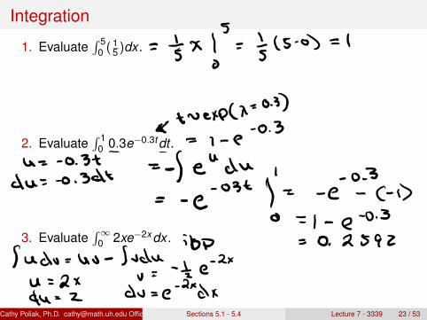
Integration
1. Evaluate∫ 5
0 (15)dx .
2. Evaluate∫ 1
0 0.3e−0.3tdt .
3. Evaluate∫∞
0 2xe−2xdx .
Cathy Poliak, Ph.D. [email protected] Office in 11c Flemming (Department of Mathematics University of Houston )Sections 5.1 - 5.4 Lecture 7 - 3339 23 / 53

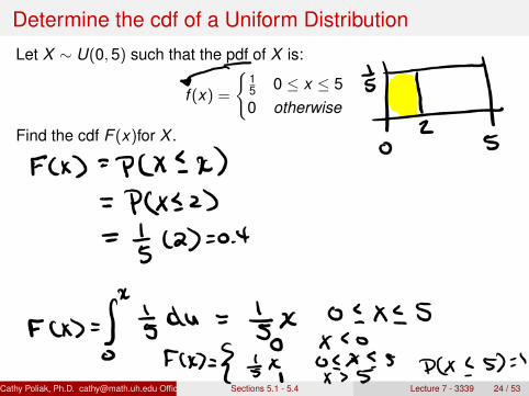
Determine the cdf of a Uniform Distribution
Let X ∼ U(0,5) such that the pdf of X is:
f (x) =
{15 0 ≤ x ≤ 50 otherwise
Find the cdf F (x)for X .
Cathy Poliak, Ph.D. [email protected] Office in 11c Flemming (Department of Mathematics University of Houston )Sections 5.1 - 5.4 Lecture 7 - 3339 24 / 53

Cumulative Density Function
0 1 2 3 4 5
0.0
0.2
0.4
0.6
0.8
1.0
X
Cum
ulat
ive
Pro
babi
lity
Cathy Poliak, Ph.D. [email protected] Office in 11c Flemming (Department of Mathematics University of Houston )Sections 5.1 - 5.4 Lecture 7 - 3339 25 / 53

Using the cdf F (X ) to Compute Probabilities
Let X be a continuous random variable with pdf f (x) and cdf F (x).Then for any number a,
P(X > a) = 1− F (a)
and for any two numbers a and b with a < b,
P(a ≤ X ≤ b) = F (b)− F (a)
Cathy Poliak, Ph.D. [email protected] Office in 11c Flemming (Department of Mathematics University of Houston )Sections 5.1 - 5.4 Lecture 7 - 3339 26 / 53

Example Using CDF
Suppose we have a cdf;
F (x) =
0, x ≤ −1x3+1
9 , −1 ≤ x < 21, x ≥ 2.
1. Determine P(X ≤ 0)
2. Determine P(0 < X ≤ 1)
3. Determine P(X ≥ 0.5)
4. Given this CDF determine the pdf f (x).Cathy Poliak, Ph.D. [email protected] Office in 11c Flemming (Department of Mathematics University of Houston )Sections 5.1 - 5.4 Lecture 7 - 3339 27 / 53
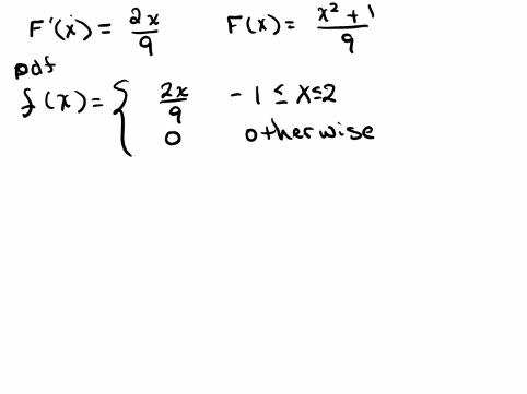

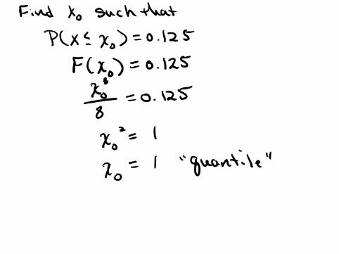
Example
Suppose we have a pdf of
f (x) =
{38x2 0 ≤ X ≤ k0 otherwise
a) Determine k .
b) Give the cdf of this distribution.
c) Determine x0 such that P(X ≤ x0) = 0.125
Cathy Poliak, Ph.D. [email protected] Office in 11c Flemming (Department of Mathematics University of Houston )Sections 5.1 - 5.4 Lecture 7 - 3339 28 / 53

Quantiles
Let F be a given cumulative distribution and let p be any real numberbetween 0 and 1. The (100p)th percentile of the distribution of acontinuous random variable X is defined as
F−1(p) = min{x |F (x) ≥ p}.
For continuous distributions, F−1(p) is the smallest number x such thatF (x) = p.
Cathy Poliak, Ph.D. [email protected] Office in 11c Flemming (Department of Mathematics University of Houston )Sections 5.1 - 5.4 Lecture 7 - 3339 29 / 53

Determine the Percentiles
Given a cdf,
F (x) =
0 X < 018x3 0 ≤ X ≤ 21 X > 2
1. Determine the 90th percentile.
2. Determine the 50th percentile.
3. Find the value of c such that P(X ≤ c) = 0.75.
Cathy Poliak, Ph.D. [email protected] Office in 11c Flemming (Department of Mathematics University of Houston )Sections 5.1 - 5.4 Lecture 7 - 3339 30 / 53
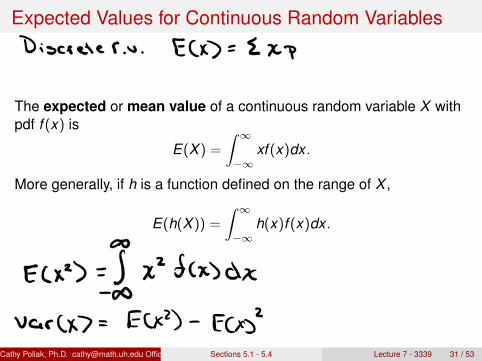
Expected Values for Continuous Random Variables
The expected or mean value of a continuous random variable X withpdf f (x) is
E(X ) =
∫ ∞−∞
xf (x)dx .
More generally, if h is a function defined on the range of X ,
E(h(X )) =
∫ ∞−∞
h(x)f (x)dx .
Cathy Poliak, Ph.D. [email protected] Office in 11c Flemming (Department of Mathematics University of Houston )Sections 5.1 - 5.4 Lecture 7 - 3339 31 / 53

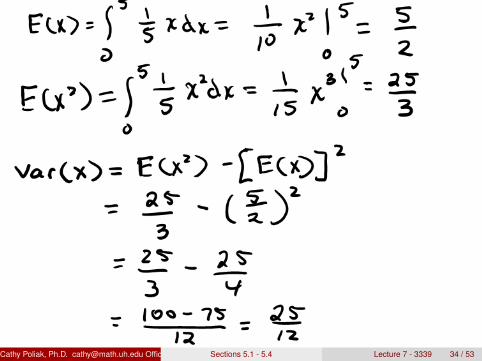
Example
The following is a pdf of X ,
f (x) =
{32(1− x2) 0 ≤ X ≤ 10 otherwise
1. Determine E(X ).
2. Determine E(X 2)
Cathy Poliak, Ph.D. [email protected] Office in 11c Flemming (Department of Mathematics University of Houston )Sections 5.1 - 5.4 Lecture 7 - 3339 32 / 53


Mean and Variance of the Uniform Distribution
Let X ∼ Unif(a,b)
E(X ) = a+b2
Var(X ) = (b−a)2
12
Cathy Poliak, Ph.D. [email protected] Office in 11c Flemming (Department of Mathematics University of Houston )Sections 5.1 - 5.4 Lecture 7 - 3339 33 / 53
Cathy Poliak, Ph.D. [email protected] Office in 11c Flemming (Department of Mathematics University of Houston )Sections 5.1 - 5.4 Lecture 7 - 3339 34 / 53

Example From Quiz 7
Let X be the amount of time (in hours) the wait is to get a table at arestaurant. Suppose the cdf is represented by
F (X ) =
0 x < 0x2
9 0 ≤ x ≤ 31 x > 3
Use the cdf to determine E[X].
Cathy Poliak, Ph.D. [email protected] Office in 11c Flemming (Department of Mathematics University of Houston )Sections 5.1 - 5.4 Lecture 7 - 3339 36 / 53

The Exponential Distribution
X is said to have an exponential distribution with parameter λ(λ > 0) if the pdf of X is:
f (x) =
{λe−λx x ≥ 00 otherwise
Where λ is a rate parameter, we write X ∼ Exp(λ). The cdf of aexponential random variable is:
F (x) =
{0 x < 01− e−λx x ≥ 0
The mean of the exponential distribution is µx = E(X ) = 1λ the
standard deviation is also 1λ .
Cathy Poliak, Ph.D. [email protected] Office in 11c Flemming (Department of Mathematics University of Houston )Sections 5.1 - 5.4 Lecture 7 - 3339 37 / 53

Exponential Density Curves
0 2 4 6 8 10
0.0
0.5
1.0
1.5
2.0
Exponential Density Curves
0 2 4 6 8 10
0.0
0.5
1.0
1.5
2.0
Exponential Density Curves
0 2 4 6 8 10
0.0
0.5
1.0
1.5
2.0
Exponential Density Curves
lambda = 0.5lambda = 1lambda = 2
lambda = 0.5lambda = 1lambda = 2
Cathy Poliak, Ph.D. [email protected] Office in 11c Flemming (Department of Mathematics University of Houston )Sections 5.1 - 5.4 Lecture 7 - 3339 38 / 53

Exponential Distribution Related to the PoissonDistribution
The exponential distribution is frequently used as a model for thedistribution of times between the occurrence of successive events untilthe first arrival.
Suppose that the number of events occurring in any time of length t hasa Poisson distribution with parameter αt .
Where α, the rate of the event process, is the expected number ofevents occurring in 1 unit of time.
The number of occurrences are in non overlapping intervals and areindependent of one another.
Then the distribution of elapsed time between the occurrence of twosuccessive events is exponential with parameter λ = α.
Cathy Poliak, Ph.D. [email protected] Office in 11c Flemming (Department of Mathematics University of Houston )Sections 5.1 - 5.4 Lecture 7 - 3339 39 / 53

Example
Suppose you usually get 3 phone calls per hour.3 phone calls per hour means that we would expect one phonecall every 1
3 hour so λ = 13 .
Compute the probability that a phone call will arrive within the nexthour.
Cathy Poliak, Ph.D. [email protected] Office in 11c Flemming (Department of Mathematics University of Houston )Sections 5.1 - 5.4 Lecture 7 - 3339 40 / 53
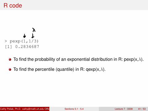
R code
> pexp(1,1/3)[1] 0.2834687
To find the probability of an exponential distribution in R: pexp(x,λ).
To find the percentile (quantile) in R: qexp(x,λ).
Cathy Poliak, Ph.D. [email protected] Office in 11c Flemming (Department of Mathematics University of Houston )Sections 5.1 - 5.4 Lecture 7 - 3339 41 / 53

Examples
Applications of the exponential distribution occurs naturally whendescribing the waiting time in a homogeneous Poisson process. It canbe used in a range of disciplines including queuing theory, physics,reliability theory, and hydrology. Examples of events that may bemodeled by exponential distribution include:
The time until a radioactive particle decaysThe time between clicks of a Geiger counterThe time until default on payment to company debt holdersThe distance between roadkills on a given roadThe distance between mutations on a DNA strandThe time it takes for a bank teller to serve a customerThe height of various molecules in a gas at a fixed temperatureand pressure in a uniform gravitational fieldThe monthly and annual maximum values of daily rainfall and riverdischarge volumes
Cathy Poliak, Ph.D. [email protected] Office in 11c Flemming (Department of Mathematics University of Houston )Sections 5.1 - 5.4 Lecture 7 - 3339 42 / 53

Example from Quiz 7
1. Suppose the time a child spends waiting at for the bus as a schoolbus stop is exponentially distributed with mean 6 minutes.Determine the probability that the child must wait at least 9minutes on the bus on a given morning.
2. Suppose the time a child spends waiting at for the bus as a schoolbus stop is exponentially distributed with mean 4 minutes.Determine the probability that the child must wait between 3 and 6minutes on the bus on a given morning.
Cathy Poliak, Ph.D. [email protected] Office in 11c Flemming (Department of Mathematics University of Houston )Sections 5.1 - 5.4 Lecture 7 - 3339 43 / 53

The "Memoryless" Property
Another application of the exponential distribution is to model thedistribution of component lifetime.
Suppose component lifetime is exponentially distributed withparameter λ.After putting the component into service, we leave for a period oft0 hours and then return to find the components still working; whatnow is the probability that it last at least an addition t hours?We want to find P(X ≥ t + t0|X ≥ t0)
Cathy Poliak, Ph.D. [email protected] Office in 11c Flemming (Department of Mathematics University of Houston )Sections 5.1 - 5.4 Lecture 7 - 3339 44 / 53

The Gamma Function
The gamma function Γ(α) is defined by:
Γ(α) =
∫ ∞0
xα−1e−xdx
Cathy Poliak, Ph.D. [email protected] Office in 11c Flemming (Department of Mathematics University of Houston )Sections 5.1 - 5.4 Lecture 7 - 3339 45 / 53

Properties of the Gamma Function
The most important properties of the gamma function are thefollowing:
1. For any α > 1, Γ(α) = (α− 1)Γ(α− 1)
2. For any positive integer, n, Γ(n) = (n − 1)!
3. Γ(12) =
√π
Cathy Poliak, Ph.D. [email protected] Office in 11c Flemming (Department of Mathematics University of Houston )Sections 5.1 - 5.4 Lecture 7 - 3339 46 / 53

The PDF of a Gamma Distribution
A continuous random variable X is said to have a gamma distributionif the pdf of X is
f (x ;α, β) =
{1
βαΓ(α)xα−1e−x/β x ≥ 0
0 otherwise
where parameters α and β satisfy α > 0, β > 0.
Cathy Poliak, Ph.D. [email protected] Office in 11c Flemming (Department of Mathematics University of Houston )Sections 5.1 - 5.4 Lecture 7 - 3339 47 / 53

Gamma Distribution Related to the Poisson
Gamma distribution is a distribution that arises naturally inprocesses for which the waiting times between events arerelevant.
It can be thought of as a waiting time between Poisson distributedevents, unitl k arrivals.
Thus the scale parameter can also be thought of as the inverse ofthe rate parameter (µ), 1
µ .
Then α = k and β = 1µ
In R, P(X ≤ x) = pgamma(x , α, 1β )
Cathy Poliak, Ph.D. [email protected] Office in 11c Flemming (Department of Mathematics University of Houston )Sections 5.1 - 5.4 Lecture 7 - 3339 48 / 53

Gamma Density Curve
0 2 4 6 8 10
0.0
0.2
0.4
0.6
0.8
1.0
Gamma Density Curve
0 2 4 6 8 10
0.0
0.2
0.4
0.6
0.8
1.0
Gamma Density Curve
0 2 4 6 8 10
0.0
0.2
0.4
0.6
0.8
1.0
Gamma Density Curve
0 2 4 6 8 10
0.0
0.2
0.4
0.6
0.8
1.0
Gamma Density Curve
alpha = 2, beta = 1/3alpa = 1, beta = 1alpha = 2, beta = 2alpha = 2, beta = 1
Cathy Poliak, Ph.D. [email protected] Office in 11c Flemming (Department of Mathematics University of Houston )Sections 5.1 - 5.4 Lecture 7 - 3339 49 / 53

Applications of the Gamma Distribution
The gamma distribution can be used a range of disciplines includingqueuing models, climatology, and financial services. Examples ofevents that may be modeled by gamma distribution include:
The amount of rainfall accumulated in a reservoir
The size of loan defaults or aggregate insurance claims
The flow of items through manufacturing and distributionprocesses
The load on web servers
The many and varied forms of telecom exchange
Cathy Poliak, Ph.D. [email protected] Office in 11c Flemming (Department of Mathematics University of Houston )Sections 5.1 - 5.4 Lecture 7 - 3339 50 / 53

Example
Suppose that the telephone calls arriving at a particular switchboardfollow a Poisson process with an average of 5 calls coming per minute.What is the probability that up to a minute will elapse until 2 calls havecome in to the switchboard?
Average of 5 calls coming per minute means that β = 15 .
Until 2 calls have come into the switchboard means that α = 2.
Cathy Poliak, Ph.D. [email protected] Office in 11c Flemming (Department of Mathematics University of Houston )Sections 5.1 - 5.4 Lecture 7 - 3339 51 / 53

Mean and Variance of the Gamma Distribution
The mean and variance of a random variable X having the gammadistribution are:
E(X ) = µ = αβ
Var(X ) = σ2 = αβ2
Cathy Poliak, Ph.D. [email protected] Office in 11c Flemming (Department of Mathematics University of Houston )Sections 5.1 - 5.4 Lecture 7 - 3339 52 / 53

Example of Gamma Distribution
Suppose that a transistor of a certain type is subjected to anaccelerated life test, the lifetime Y (in weeks) has a gamma distributionwith a mean of 24 and a standard deviation of 12.
1. Find the values of α and β.
2. Find P(Y ≤ 24)
Cathy Poliak, Ph.D. [email protected] Office in 11c Flemming (Department of Mathematics University of Houston )Sections 5.1 - 5.4 Lecture 7 - 3339 53 / 53