section 4.4 cathy poliak, ph.d. [email protected] office ...cathy/math2311/lectures... · a. 2 b....
TRANSCRIPT
Sampling Distributions of x̄ and p̂Section 4.4
Cathy Poliak, [email protected]
Office hours: T Th 2:30 - 5:15 pm 620 PGH
Department of MathematicsUniversity of Houston
February 25, 2016
Cathy Poliak, Ph.D. [email protected] Office hours: T Th 2:30 - 5:15 pm 620 PGH (Department of Mathematics University of Houston )Section 4.4 February 25, 2016 1 / 35
Outline
1 Beginning Questions
2 Sampling Distribution of X̄
3 Unbiased Estimate
4 Finding Probabilities for X̄
5 Proportions
6 Sampling Distribution of p̂
Cathy Poliak, Ph.D. [email protected] Office hours: T Th 2:30 - 5:15 pm 620 PGH (Department of Mathematics University of Houston )Section 4.4 February 25, 2016 2 / 35
Popper Set Up
Fill in all of the proper bubbles.
Use a #2 pencil.
This is popper number 08.
Cathy Poliak, Ph.D. [email protected] Office hours: T Th 2:30 - 5:15 pm 620 PGH (Department of Mathematics University of Houston )Section 4.4 February 25, 2016 3 / 35
Popper Questions
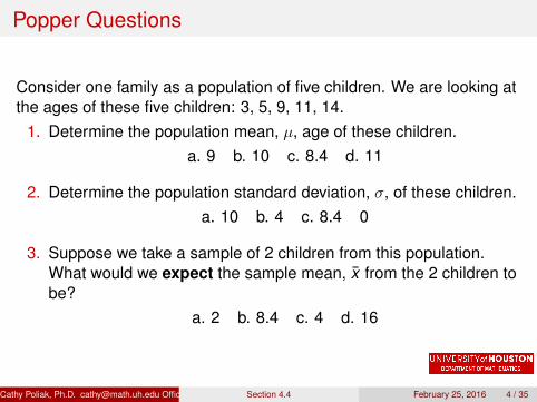
Consider one family as a population of five children. We are looking atthe ages of these five children: 3, 5, 9, 11, 14.
1. Determine the population mean, µ, age of these children.a. 9 b. 10 c. 8.4 d. 11
2. Determine the population standard deviation, σ, of these children.a. 10 b. 4 c. 8.4 0
3. Suppose we take a sample of 2 children from this population.What would we expect the sample mean, x̄ from the 2 children tobe?
a. 2 b. 8.4 c. 4 d. 16
Cathy Poliak, Ph.D. [email protected] Office hours: T Th 2:30 - 5:15 pm 620 PGH (Department of Mathematics University of Houston )Section 4.4 February 25, 2016 4 / 35
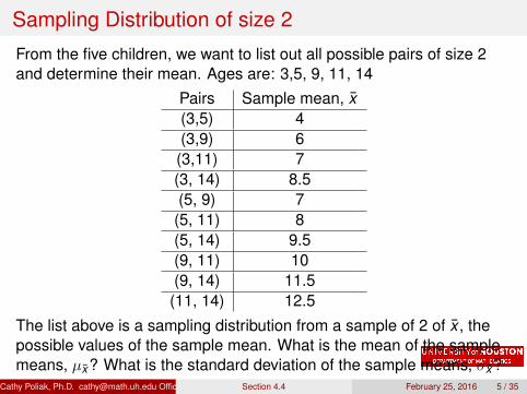
Sampling Distribution of size 2
From the five children, we want to list out all possible pairs of size 2and determine their mean. Ages are: 3,5, 9, 11, 14
Pairs Sample mean, x̄(3,5) 4(3,9) 6(3,11) 7(3, 14) 8.5(5, 9) 7
(5, 11) 8(5, 14) 9.5(9, 11) 10(9, 14) 11.5(11, 14) 12.5
The list above is a sampling distribution from a sample of 2 of x̄ , thepossible values of the sample mean. What is the mean of the samplemeans, µx̄? What is the standard deviation of the sample means, σx̄?
Cathy Poliak, Ph.D. [email protected] Office hours: T Th 2:30 - 5:15 pm 620 PGH (Department of Mathematics University of Houston )Section 4.4 February 25, 2016 5 / 35
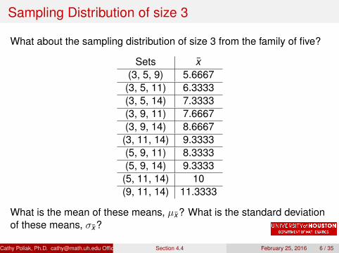
Sampling Distribution of size 3
What about the sampling distribution of size 3 from the family of five?
Sets x̄(3, 5, 9) 5.6667(3, 5, 11) 6.3333(3, 5, 14) 7.3333(3, 9, 11) 7.6667(3, 9, 14) 8.6667
(3, 11, 14) 9.3333(5, 9, 11) 8.3333(5, 9, 14) 9.3333
(5, 11, 14) 10(9, 11, 14) 11.3333
What is the mean of these means, µx̄? What is the standard deviationof these means, σx̄?
Cathy Poliak, Ph.D. [email protected] Office hours: T Th 2:30 - 5:15 pm 620 PGH (Department of Mathematics University of Houston )Section 4.4 February 25, 2016 6 / 35
Sampling distribution
When we describe distributions we use three characteristics:I ShapeI CenterI Spread
To describe the sampling distribution we can use the same threecharacteristics.
This can be shown through histograms or numerical values.
Cathy Poliak, Ph.D. [email protected] Office hours: T Th 2:30 - 5:15 pm 620 PGH (Department of Mathematics University of Houston )Section 4.4 February 25, 2016 7 / 35
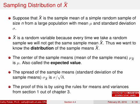
Sampling Distribution of X̄
Suppose that X̄ is the sample mean of a simple random sample ofsize n from a large population with mean µ and standard deviationσ.
X̄ is a random variable because every time we take a randomsample we will not get the same sample mean X̄ . Thus we want toknow the distribution of the sample means X̄ .
The center of the sample means (mean of the sample means) µX̄is µ. Also called the expected value.
The spread of the sample means (standard deviation of thesample means) σX̄ is σ/
√n.
The proof of this is by using the rules for means and variancesfrom section 1 out of chapter 3.
Cathy Poliak, Ph.D. [email protected] Office hours: T Th 2:30 - 5:15 pm 620 PGH (Department of Mathematics University of Houston )Section 4.4 February 25, 2016 8 / 35
Popper Questions
For each of the following scenarios is the bold numbera. parameter or b. statistic?
4. A television station is interested in predicting whether voters intheir listening area are in favor of federal funding for abortions. Itasks its viewers to phone in and indicate whether they are in favoror opposed to this. Of the 2241 viewers who phoned in, 1574(70.24%) were opposed to federal funding for abortions.
5. Every five years, Statistics Canada conducts a Census ofAgriculture. The target of the census is all farms selling one ormore agricultural products. In 2006, Statistics Canada reportedthat the average age of a farmer on Prince Edward Island was51.4 years old.
Cathy Poliak, Ph.D. [email protected] Office hours: T Th 2:30 - 5:15 pm 620 PGH (Department of Mathematics University of Houston )Section 4.4 February 25, 2016 9 / 35
Estimating parameters
As an estimation of the parameters we use their correspondingstatistics.
The parameters we will estimate in this course is the populationmean µ, the population proportion p and the regressionparameters β.
The statistics are random variables. Meaning, if we take differentrandom samples we will get different values for the sample meanX̄ sample proportion p̂ and sample regression estimates b0 or b1.
The sampling distribution of a statistic is the "ideal" distributionof values taken by the statistic in all possible samples of the samesize from the same population.
If the mean of the sampling distribution is the same as the meanof the population then our estimate is considered to be andunbiased estimate.
Cathy Poliak, Ph.D. [email protected] Office hours: T Th 2:30 - 5:15 pm 620 PGH (Department of Mathematics University of Houston )Section 4.4 February 25, 2016 10 / 35
Sampling Distribution Example
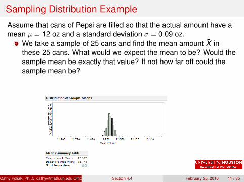
Assume that cans of Pepsi are filled so that the actual amount have amean µ = 12 oz and a standard deviation σ = 0.09 oz.
We take a sample of 25 cans and find the mean amount X̄ inthese 25 cans. What would we expect the mean to be? Would thesample mean be exactly that value? If not how far off could thesample mean be?
Cathy Poliak, Ph.D. [email protected] Office hours: T Th 2:30 - 5:15 pm 620 PGH (Department of Mathematics University of Houston )Section 4.4 February 25, 2016 11 / 35
Sampling Distribution Example
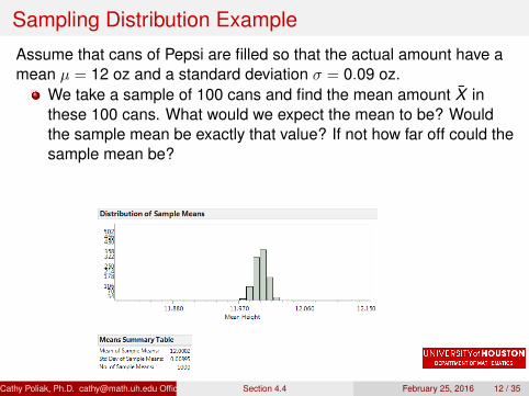
Assume that cans of Pepsi are filled so that the actual amount have amean µ = 12 oz and a standard deviation σ = 0.09 oz.
We take a sample of 100 cans and find the mean amount X̄ inthese 100 cans. What would we expect the mean to be? Wouldthe sample mean be exactly that value? If not how far off could thesample mean be?
Cathy Poliak, Ph.D. [email protected] Office hours: T Th 2:30 - 5:15 pm 620 PGH (Department of Mathematics University of Houston )Section 4.4 February 25, 2016 12 / 35
Shape of the Sample Mean Distribution
If a population has a Normal distribution, then the sample mean X̄of n independent observations also has a Normal distribution withmean µ and standard deviation σ/
√n.
Central limit theorem: For any population, when n is large(n > 30), the sampling distribution of the sample mean X̄ isapproximately a Normal distribution with mean µ and standarddeviation σ/
√n.
Cathy Poliak, Ph.D. [email protected] Office hours: T Th 2:30 - 5:15 pm 620 PGH (Department of Mathematics University of Houston )Section 4.4 February 25, 2016 13 / 35
Example: Amount of Pepsi
Assume that cans of Pepsi are filled so that the actual amount have amean µ = 12 oz and a standard deviation σ = 0.09 oz. Suppose that arandom sample of 4 cans are examined, describe the distribution ofthe sample means X̄ .
Center: µX̄ = µ = 12Spread: σX̄ = σ√
n = 0.09√4
= 0.045
Shape: Unknown because we do not know the original distributionand the sample size is small.
Cathy Poliak, Ph.D. [email protected] Office hours: T Th 2:30 - 5:15 pm 620 PGH (Department of Mathematics University of Houston )Section 4.4 February 25, 2016 14 / 35
Example: Amount of Pepsi
Assume that cans of Pepsi are filled so that the actual amount have amean µ = 12 oz and a standard deviation σ = 0.09 oz. Suppose that arandom sample of 100 cans are examined, describe the distribution ofthe sample means X̄ .
Center: µX̄ = µ = 12Spread: σX̄ = σ√
n = 0.09√100
= 0.009
Shape: Normal because we have a large sample thus we canapply the Central Limit Theorem.
Cathy Poliak, Ph.D. [email protected] Office hours: T Th 2:30 - 5:15 pm 620 PGH (Department of Mathematics University of Houston )Section 4.4 February 25, 2016 15 / 35
Finding Probabilities
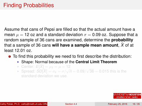
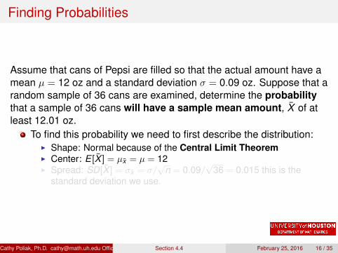
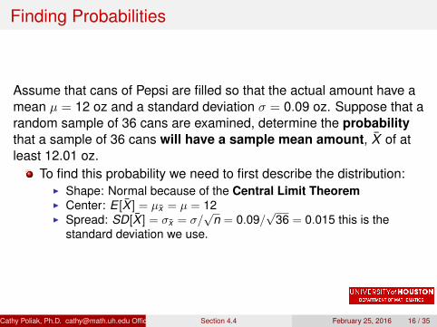
Assume that cans of Pepsi are filled so that the actual amount have amean µ = 12 oz and a standard deviation σ = 0.09 oz. Suppose that arandom sample of 36 cans are examined, determine the probabilitythat a sample of 36 cans will have a sample mean amount, X̄ of atleast 12.01 oz.
To find this probability we need to first describe the distribution:I Shape: Normal because of the Central Limit TheoremI Center: E [X̄ ] = µx̄ = µ = 12I Spread: SD[X̄ ] = σx̄ = σ/
√n = 0.09/
√36 = 0.015 this is the
standard deviation we use.
Cathy Poliak, Ph.D. [email protected] Office hours: T Th 2:30 - 5:15 pm 620 PGH (Department of Mathematics University of Houston )Section 4.4 February 25, 2016 16 / 35
Finding Probabilities
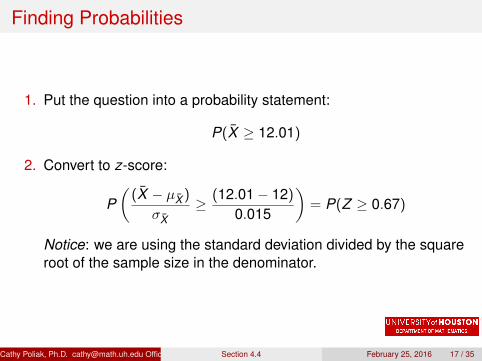
1. Put the question into a probability statement:
P(X̄ ≥ 12.01)
2. Convert to z-score:
P(
(X̄ − µX̄ )
σX̄≥ (12.01− 12)
0.015
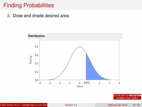
)= P(Z ≥ 0.67)
Notice: we are using the standard deviation divided by the squareroot of the sample size in the denominator.
Cathy Poliak, Ph.D. [email protected] Office hours: T Th 2:30 - 5:15 pm 620 PGH (Department of Mathematics University of Houston )Section 4.4 February 25, 2016 17 / 35
Finding Probabilities
3. Draw and shade desired area.
0.67
Cathy Poliak, Ph.D. [email protected] Office hours: T Th 2:30 - 5:15 pm 620 PGH (Department of Mathematics University of Houston )Section 4.4 February 25, 2016 18 / 35
Finding Probabilities
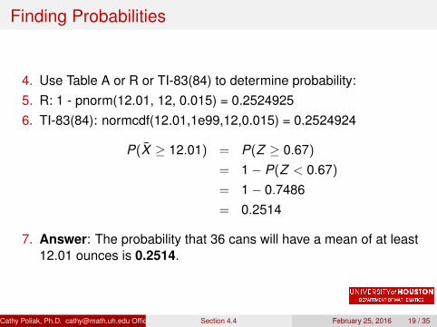
4. Use Table A or R or TI-83(84) to determine probability:5. R: 1 - pnorm(12.01, 12, 0.015) = 0.25249256. TI-83(84): normcdf(12.01,1e99,12,0.015) = 0.2524924
P(X̄ ≥ 12.01) = P(Z ≥ 0.67)
= 1− P(Z < 0.67)
= 1− 0.7486= 0.2514
7. Answer: The probability that 36 cans will have a mean of at least12.01 ounces is 0.2514.
Cathy Poliak, Ph.D. [email protected] Office hours: T Th 2:30 - 5:15 pm 620 PGH (Department of Mathematics University of Houston )Section 4.4 February 25, 2016 19 / 35
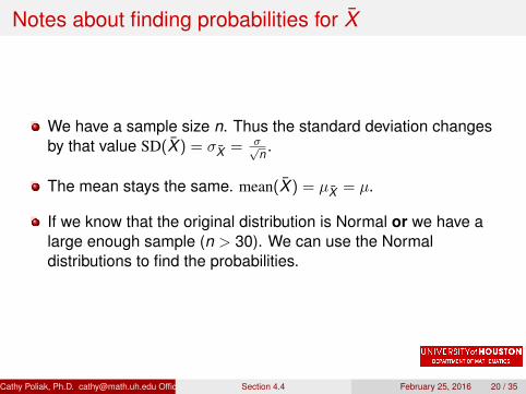
Notes about finding probabilities for X̄
We have a sample size n. Thus the standard deviation changesby that value SD(X̄ ) = σX̄ = σ√
n .
The mean stays the same. mean(X̄ ) = µX̄ = µ.
If we know that the original distribution is Normal or we have alarge enough sample (n > 30). We can use the Normaldistributions to find the probabilities.
Cathy Poliak, Ph.D. [email protected] Office hours: T Th 2:30 - 5:15 pm 620 PGH (Department of Mathematics University of Houston )Section 4.4 February 25, 2016 20 / 35
Popper Questions
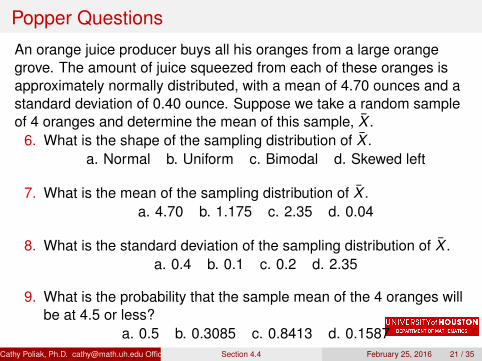
An orange juice producer buys all his oranges from a large orangegrove. The amount of juice squeezed from each of these oranges isapproximately normally distributed, with a mean of 4.70 ounces and astandard deviation of 0.40 ounce. Suppose we take a random sampleof 4 oranges and determine the mean of this sample, X̄ .
6. What is the shape of the sampling distribution of X̄ .a. Normal b. Uniform c. Bimodal d. Skewed left
7. What is the mean of the sampling distribution of X̄ .a. 4.70 b. 1.175 c. 2.35 d. 0.04
8. What is the standard deviation of the sampling distribution of X̄ .a. 0.4 b. 0.1 c. 0.2 d. 2.35
9. What is the probability that the sample mean of the 4 oranges willbe at 4.5 or less?
a. 0.5 b. 0.3085 c. 0.8413 d. 0.1587Cathy Poliak, Ph.D. [email protected] Office hours: T Th 2:30 - 5:15 pm 620 PGH (Department of Mathematics University of Houston )Section 4.4 February 25, 2016 21 / 35
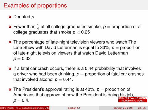
Examples of proportions
Denoted p.
Fewer than 14 of all college graduates smoke, p = proportion of all
college graduates that smoke p < 0.25
The percentage of late-night television viewers who watch TheLate Show with David Letterman is equal to 33%, p = proportionof late-night television viewers that watch David Lettermanp = 0.33
If a fatal car crash occurs, there is a 0.44 probability that involvesa driver who had been drinking, p = proportion of fatal car crashesthat involved alcohol p = 0.44.
The President’s approval rating is at 40%, p = proportion ofAmericans that approve of how the President is doing his job,p = 0.4.
Cathy Poliak, Ph.D. [email protected] Office hours: T Th 2:30 - 5:15 pm 620 PGH (Department of Mathematics University of Houston )Section 4.4 February 25, 2016 22 / 35
Sample Proportions
The population proportion is p a parameter. In some cases we donot know the population proportion, thus we use the sampleproportion, p̂ to estimate p.
The sample proportion is calculated by: p̂ = Xn
X = the number of observations of interest in the sample or thenumber of "successes" in the sample.
n = the sample size or number of observations.
Cathy Poliak, Ph.D. [email protected] Office hours: T Th 2:30 - 5:15 pm 620 PGH (Department of Mathematics University of Houston )Section 4.4 February 25, 2016 23 / 35
Example
According to the National Retail Federation, 34% of taxpayersused computer software to do their taxes.
A sample of 50 taxpayers was selected what do we expect thesample proportion p̂ to be?
Of we take other samples will the sample proportions always bethe same value?
If not what would p̂ be off by?
Cathy Poliak, Ph.D. [email protected] Office hours: T Th 2:30 - 5:15 pm 620 PGH (Department of Mathematics University of Houston )Section 4.4 February 25, 2016 24 / 35
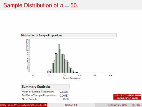
Sample Distribution of n = 50.
Cathy Poliak, Ph.D. [email protected] Office hours: T Th 2:30 - 5:15 pm 620 PGH (Department of Mathematics University of Houston )Section 4.4 February 25, 2016 25 / 35
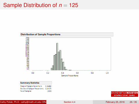
Sample Distribution of n = 125
Cathy Poliak, Ph.D. [email protected] Office hours: T Th 2:30 - 5:15 pm 620 PGH (Department of Mathematics University of Houston )Section 4.4 February 25, 2016 26 / 35
Shape of the distribution of p̂
Notice from the previous histograms that it appears to have aNormal distribution.We can use the Normal distribution as long as np ≥ 10 thenumber of successes are at least 10 and n(1− p) ≥ 10 thenumber of failures are at least 10.
Cathy Poliak, Ph.D. [email protected] Office hours: T Th 2:30 - 5:15 pm 620 PGH (Department of Mathematics University of Houston )Section 4.4 February 25, 2016 27 / 35
Center of the distribution of p̂
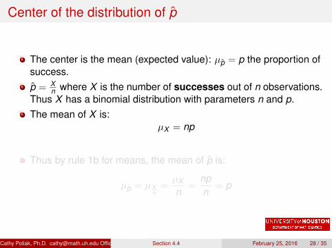
The center is the mean (expected value): µp̂ = p the proportion ofsuccess.p̂ = X
n where X is the number of successes out of n observations.Thus X has a binomial distribution with parameters n and p.The mean of X is:
µX = np
Thus by rule 1b for means, the mean of p̂ is:
µp̂ = µ Xn
=µX
n=
npn
= p
Cathy Poliak, Ph.D. [email protected] Office hours: T Th 2:30 - 5:15 pm 620 PGH (Department of Mathematics University of Houston )Section 4.4 February 25, 2016 28 / 35
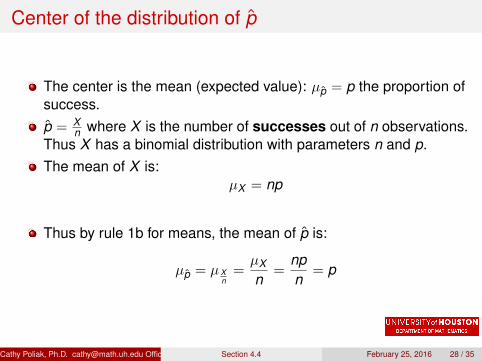
Center of the distribution of p̂
The center is the mean (expected value): µp̂ = p the proportion ofsuccess.p̂ = X
n where X is the number of successes out of n observations.Thus X has a binomial distribution with parameters n and p.The mean of X is:
µX = np
Thus by rule 1b for means, the mean of p̂ is:
µp̂ = µ Xn
=µX
n=
npn
= p
Cathy Poliak, Ph.D. [email protected] Office hours: T Th 2:30 - 5:15 pm 620 PGH (Department of Mathematics University of Houston )Section 4.4 February 25, 2016 28 / 35
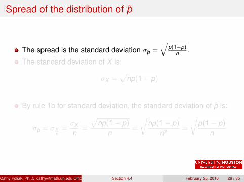
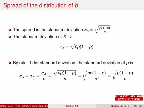
Spread of the distribution of p̂
The spread is the standard deviation σp̂ =√
p(1−p)n .
The standard deviation of X is:
σX =√
np(1− p)
By rule 1b for standard deviation, the standard deviation of p̂ is:
σp̂ = σ Xn
=σX
n=
√np(1− p)
n=
√np(1− p)
n2 =
√p(1− p)
n
Cathy Poliak, Ph.D. [email protected] Office hours: T Th 2:30 - 5:15 pm 620 PGH (Department of Mathematics University of Houston )Section 4.4 February 25, 2016 29 / 35
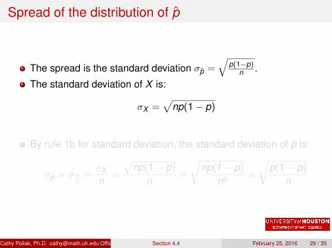
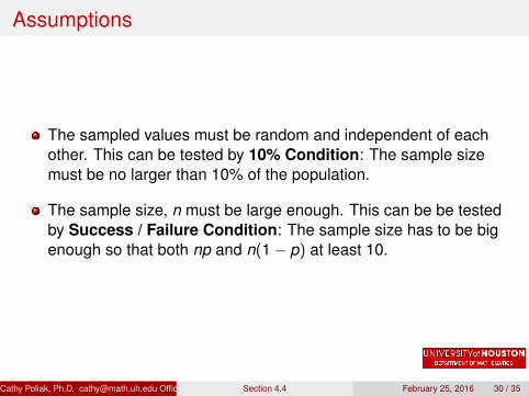
Assumptions
The sampled values must be random and independent of eachother. This can be tested by 10% Condition: The sample sizemust be no larger than 10% of the population.
The sample size, n must be large enough. This can be be testedby Success / Failure Condition: The sample size has to be bigenough so that both np and n(1− p) at least 10.
Cathy Poliak, Ph.D. [email protected] Office hours: T Th 2:30 - 5:15 pm 620 PGH (Department of Mathematics University of Houston )Section 4.4 February 25, 2016 30 / 35
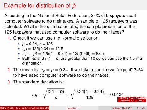
Example for distribution of p̂
According to the National Retail Federation, 34% of taxpayers usedcomputer software to do their taxes. A sample of 125 taxpayers wasselected. What is the distribution of p̂, the sample proportion of the125 taxpayers that used computer software to do their taxes?
1. Check if we can use the Normal distribution.I p = 0.34, n = 125I np = 125(0.34) = 42.5I n(1− p) = 125(1− 0.34) = 125(0.66) = 82.5I Both np and n(1− p) are greater than 10 so we can use the Normal
distribution.
2. The mean is: µp̂ = p = 0.34. If we take a sample we "expect" 34%to have used computer software to do their taxes.
3. The standard deviation is:
σp̂ =
√p(1− p)
n=
√0.34(1− 0.34)
125= 0.0424
Cathy Poliak, Ph.D. [email protected] Office hours: T Th 2:30 - 5:15 pm 620 PGH (Department of Mathematics University of Houston )Section 4.4 February 25, 2016 31 / 35
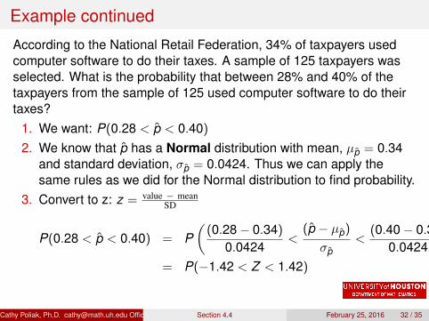
Example continued
According to the National Retail Federation, 34% of taxpayers usedcomputer software to do their taxes. A sample of 125 taxpayers wasselected. What is the probability that between 28% and 40% of thetaxpayers from the sample of 125 used computer software to do theirtaxes?
1. We want: P(0.28 < p̂ < 0.40)
2. We know that p̂ has a Normal distribution with mean, µp̂ = 0.34and standard deviation, σp̂ = 0.0424. Thus we can apply thesame rules as we did for the Normal distribution to find probability.
3. Convert to z: z = value − meanSD
P(0.28 < p̂ < 0.40) = P(
(0.28− 0.34)
0.0424<
(p̂ − µp̂)
σp̂<
(0.40− 0.34)
0.0424
)= P(−1.42 < Z < 1.42)
Cathy Poliak, Ph.D. [email protected] Office hours: T Th 2:30 - 5:15 pm 620 PGH (Department of Mathematics University of Houston )Section 4.4 February 25, 2016 32 / 35
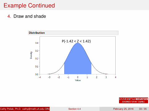
Example Continued
4. Draw and shade
P(-1.42 < Z < 1.42)
Cathy Poliak, Ph.D. [email protected] Office hours: T Th 2:30 - 5:15 pm 620 PGH (Department of Mathematics University of Houston )Section 4.4 February 25, 2016 33 / 35
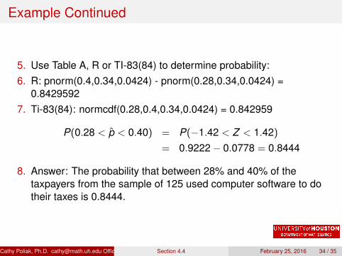
Example Continued
5. Use Table A, R or TI-83(84) to determine probability:6. R: pnorm(0.4,0.34,0.0424) - pnorm(0.28,0.34,0.0424) =
0.84295927. Ti-83(84): normcdf(0.28,0.4,0.34,0.0424) = 0.842959
P(0.28 < p̂ < 0.40) = P(−1.42 < Z < 1.42)
= 0.9222− 0.0778 = 0.8444
8. Answer: The probability that between 28% and 40% of thetaxpayers from the sample of 125 used computer software to dotheir taxes is 0.8444.
Cathy Poliak, Ph.D. [email protected] Office hours: T Th 2:30 - 5:15 pm 620 PGH (Department of Mathematics University of Houston )Section 4.4 February 25, 2016 34 / 35
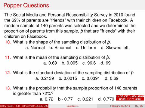
Popper Questions
The Social Media and Personal Responsibility Survey in 2010 foundthe 69% of parents are "friends" with their children on Facebook. Arandom sample of 140 parents was selected and we determined theproportion of parents from this sample, p̂ that are "friends" with theirchildren on Facebook.10. What is the shape of the sampling distribution of p̂.
a. Normal b. Binomial c. Uniform d. Skewed left
11. What is the mean of the sampling distribution of p̂.a. 0.69 b. 0.005 c. 96.6 d. 69
12. What is the standard deviation of the sampling distribution of p̂.a. 0.2139 b. 0.0015 c. 0.0391 d. 0.69
13. What is the probability that the sample proportion of 140 parentsis greater than 72%?
a. 0.72 b.- 0.77 c. 0.221 d. 0.779Cathy Poliak, Ph.D. [email protected] Office hours: T Th 2:30 - 5:15 pm 620 PGH (Department of Mathematics University of Houston )Section 4.4 February 25, 2016 35 / 35