CONTRACT NAS5-21798, "STUDIES OF SQUNDINGS AND IMAGING MEASUREMENTS

FROM GEOSTATIONARY SATELLITES"

Verner E. Suomi, DirectorThe University of WisconsinSpace Science and Engineering Center1225 West Dayton StreetMadison, Wisconsin 53706

(NASA-CR-132799) STUDIES OF SOUNDINGS N73-27761AND IMAGINGS MEASUREMENTS FROM

GEOSTATIONARY SATELLITES Quarterly

Report, 1 Feb. - 30 Apre 1973 (Wisconsin UnclasUniv.) }2zI p HC $3.25 CSCL 03B G3/31 09275

May 1973Quarterly Report for Period 1 February 1973 - 30 April 1973

Prepared for

NATIONAL AERONAUTICS AND SPACE ADMINISTRATIONGODDARD SPACE FLIGHT CENTER

Greenbelt, Maryland 20771

https://ntrs.nasa.gov/search.jsp?R=19730019029 2018-06-04T15:52:33+00:00Z

TECHNIlCAL REPORT STANDARD TITLE PAGE1. Report No. 2. Government Accession No.

4. litle ond Subtitle

STUDIES OF SOUNDINGS AND IMAGINGMEASUREMENTS FROM GEOSTATIONARY SATELLITES

7. Author(s)

Verner E. Suomi9. Performing Organization Name end AddressThe University of WisconsinSpace Science and Engineering Center1225 West Dayton StreetMadison, WI 53706

12. Sponsoring Agency Name end Address

Goddard Space Flight CenterGreenbelt, Maryland 20771

15. Supplementary Notes

16. Abstract

This is the third Quarterly Report on "Studies of Soundingsand Imaging Measurements from Geostationary Satellites."The report covers work performed during the quarter on fiverelated studies.

17. Key Words (S, lected by Author(s))

MeteorologySun GlitterCloud Growth RateSatellite StabilityHiIh ib.olUtion nLptLr

19. Security Classif. (of this report)

Unclassified

18. Distribution Statement

'For sale tby the Clcringlhousc for l:ederal Scientific and Technical Information, Springfield, \irginia 22151.

Figure 2. Technical Report Standard Title Page

3. Recipient's Catalog No.

37Report I)DatMay 1973

6. Performing Organization Code

8. Perfortming Organization Report No.

10. Work Unit No.

11. Contrcct or Gront No.

13. Type of Report and Period Covered

Quarterly Report1 February 1973n- Ansril1 e97 o -

14. Sponsoring Agency Code

-- -- -- -- - -- -

--

i

TABLE OF CONTENTS

Preface . . . . . . . . . . . . . . . . . . . . . . . .

Introduction . . . . . . . . . . . . . . . . . . .

Task Progress .....................

Task A. Investigations of Meteorological DataProcessing Techniques . . . . . . . . . .

Task B. Sun Glitter . . . .. . . . ..... . .

Task D. Cloud Growth Rate Study . . . . . . . . .

Task E. Comparative Studies in Satellite Stability

Task F. High Resolution Optics Study . . . .......

New Technology . . . . . . . . . . . . . . . . . . . . .

Program for Next Reporting Interval . . . . . . . . . .

Conclusions and Recommendations . . . . . . . . . . . .

Appendix

iv

1

3

3

7

8

13

13

14

14

17

Preface

This is the third quarterly report on Contract NAS5-21798, "Studies

of Sounding and Imaging Measurements from Geostationary Satellites."

Significant progress has been made on most tasks during the reporting

period. The prototype McIDAS equipment has continued to work well.

i.

Introduction

This third quarterly report covers work performed from 1 February 1973

through 30 April 1973. In summary, progress by task is as follows:

Task A. Investigations of Meteorological Data ProcessingTechniques

Substantial progress has been made towards correcting ATS line

start errors. This includes the development of an algorithm to

detect the right hand earth limb in very noisy ATS images and the

development of a processing technique which uses the limb detection

algorithms to correct raw ATS data. Line start errors have been

corrected on 23 ATS images, thus allowing relatively accurate wind

determination from otherwise unusable data.

Task B. Sun Glitter

Mr. Jack Kornfield, the student who has almost completed a Ph. D.

thesis on the "Determination of Sea Surface Wind and Stress from

Sunglint Observed by a Geostationary Satellite," is no longer at the

University. However, he is still working to complete the thesis.

In order to meet the University thesis requirements, it must be

completed by October. Therefore, it will be available as a final

report at that time--whether completed as a thesis or not.

Task D. Cloud Growth Rate

In a master's thesis now completed, the effects of changing

sun-satellite-cloud geometry on ATS-3 viewed cloud brightness have

been documented. The brightness contrast analyses within clouds

2

were found to depend on scattering angles. For a large cloud mass

different parts of the same clouds appeared to have different

scattering properties; hence, different normalization corrections

may be required. This suggests an important deficiency of present

normalization procedures, which apply the same correction factor for

all parts of the cloud.

Also considered were observations of the scattering phase function

and the effects of cloud breaks smaller than camera resolution. Work

is underway on the development of a normalization procedure which will

use a theoretical multiple scattering program to generate data on the

brightness of clouds with various thicknesses for varying sun-cloud-

satellite geometries.

Task E. Comparative Studies in Satellite Stability

Appendices 6 and 7 and Part VI to Das' technical report have been

completed. Part VI of the report is attached at the end of this

summary as an appendix. Complete coding of the model is proceeding

on schedule.

Task F. High Resolution Optics Study

The seminar on mesoscale monitoring and prediction has been completed.

Students have studied the causes and behavior of tornadoes, hurricanes,

heavy snow swaths, thunderstorms, hail, sleet, flash floods, clear air

turbulence, fog, and lake and sea breezes. Key observables in the

motion, thermal, and moisture fields were identified and means of

communicating such information to the local Madison community explored.

Two days of briefings were held to transmit this information from the

3

students to SSEC physicists and engineers who will complete the study

by investigating how the key observables can be measured; and, if

time permits, by broadening the scope of the seminar subjects. We

have reached two main conclusions so far: (1) SEOS will combine

attributes necessary for mesoscale study which are not found in any

other observing system, and (2) a high resolution vertical temperature

and moisture sounding capability (in addition to imaging) is required

to adequately treat mesoscale monitoring and prediction.

Operation of the McIDAS system has been virtually trouble-free. Use of

the system has been so intensive, the two primary problems over the last

few weeks have been scheduling users and near saturation of the disk

storage capacity. Certain program objectives and emphases have been shifted

to reflect the demands of the new Task F, High Resolution Optics Study.

Task Progress

Task A. Investigations of Meteorological Data Processing Techniques

During the past quarter, effort on this task has resulted in significant

progress in the correction of ATS line start errors. Specific advances include:

1. Development of an algorithm to detect the right hand earth

limb in very noisy ATS images;

2. Development of a processing technique which uses the limb

detection algorithms to correct raw ATS data; and

3. Correction of line start errors in 23 ATS images, thus allowing

relatively accurate wind determinations from otherwise unuseable

data.

Each of these items is explained in the following series of discussions.

4

Development of Right Hand Algorithm

Development of a noise compensated threshold detection algorithm

for locating an effective left hand earth edge has already been reported

on in previous quarterly reports. The difference between the left hand

and right hand edges of (some) ATS pictures is the amount of communication

noise present. This noise on the right hand side is so large (for days

203, 204, of 1969) that an entirely new algorithm was needed.

Line plots of ATS data (day 204, 1969) near the right hand limb

revealed large and frequent noise spikes both within the earth's disk

and in space. Application of a simple filter (10 sample running mean)

eliminated the spikes but did not remove lower frequency noise components.

However, further filtering was not practical because the rise of the

limb radiance profile would also be filtered out. Instead, the problem

of falsely triggering on a low frequency noise burst was largely avoided

by requiring the threshold to be exceeded at several points over a wide

sample spacing simultaneously. In other words, the edge position was

found at sample N if N was the largest sample number for which the ATS

signal exceeded the specified threshold at N, N-1, N-2, N-5, N-10, N-20,

and N-30. (A better, though more complicated procedure, would be to

find the best fit position of a theoretical profile to the data.) As in

the case of the left hand algorithm, the threshold is augmented by the

mean space noise before testing against the data.

Test runs with thresholds of 5, 10, 20, 30, and 40 were made to find

the threshold which yielded the smallest line to line variance. The 30

threshold was found to be the most stable. The lower thresholds appeared

to be quite sensitive to noise; and the higher threshold appeared to respond

to cloud cover variations. Unfortunately, it was not possible to check the

5

threshold detection results against landmark measurements (as was done

with the left hand algorithm) since no suitable landmarks were illuminated

at the same time the right hand limb was illuminated. The only further

verification available at this time is in the consistency of wind fields

derived from data corrected from the algorithm results.

Development of a Data Processing Technique

Given a measured position of the earth edge for each line of each

ATS image in a sequence, there are a number of ways in which that

information can be used to improve the accuracy of cloud motion vectors.

The method we have chosen after some experimentation is one which maintains

maximum compatibility with already existing data processing software. The

basic operations involved can be summarized as follows:

a) image navigation,

b) calculation of navigation predictions of earth edge

position as a function of line number for each image,

c) threshold detection of earth edge position as a function

of line number for each image, and

d) write new digital tapes which are identical to raw tapes

except for line shifts equal to the differences between

results of b) and c).

After d) is completed, images can be displayed and processed for wind

sets using standard techniques.

The first step (image navigation), although a standard procedure in ATS

data processing, required special procedures and software to allow use of

earth edge corrections of'line start timing errors.

6

The present procedures are being employed in processing data on

the WINDCO (prototype McIDAS) system. We plan to employ somewhat different

and more efficient procedures on the advanced McIDAS system. These will

be discussed in subsequent reports.

Data Processing Activities

In response to needs of Center scientists, corrected digital tapes

have been written for ATS-3 data from day 204, 1969 and day 203, 1969.

The corrected images are 800 line swaths encompassing the target area of

the experiment. We now have 16 such corrected images for day 204, ten

based on left hand limb detection and six based on right hand limb

detection. In addition, seven corrected images have been written for day

203, these based on left hand limb detection. Additional 203 data, as

well as 202 data, will be processed during the next quarter.

Wind sets have now been obtained for both right hand and left hand

based corrections. They show east-west residuals which are comparable

to, or less than, those obtained from raw data with low line start timing

errors. This preliminary verification that the correction procedures do

result in significant data improvement will be made more quantitative

by further tests planned for the next quarter.

7

Task B. Sun Glitter

Sun glitter studies have followed two paths: (1) an investigation of the

utility and technique of obtaining sun glitter measurements from a geostationary

satellite images, and (2) a study of the problems of geometry (pointing angle,

etc.) from a near earth orbiting satellite.

Kornfield has almost completed a Ph.D. thesis on the first subject. He

shows that one can indeed obtain excellent estimates of surface wind velocity

(we already knew we could get good estimates of wind speed) from sun glitter

measurements. There are two ways to.get the wind direction information. One

can use the mean square slope in the cross wind and the downwind directions

separately. The sunglitter intensity is a measure of the slope probability--

but it is also affected by the intervening atmosphere, scatter by the white

caps, scatter by the ocean, and also glitter arising from the sky dome. He

shows how to account for all of these and is able to get wind direction for

typical conditions, but not the very light winds or very strong winds. He has

also found--and this may be more important--that the displacement of the most

probable slope; i.e., the brightest part of the sun glitter, from the position

the sun's image would occupy if the sea were calm, is directly proportional to

the square of surface wind. Indeed, it appears to be directly proportional to

the wind stress on the sea surface. This kind of information is difficult to

extract from geostationary satellite images because they cover such a wide area.

This data would be easy to extract from near earth orbiting satellites. (Kornfield

started this work with support from another sponsor, but his support until recently

has been under this contract. Although no longer at the University, Kornfield

is continuing to write his thesis, which must by University rules be submittedly

by October 1973). There is no specific progress to report on item (2)--the

8

geometry for the near earth satellite--except that the computer programming

effort continues.

Task D. Cloud Growth Rate

A master's thesis outlining the requirements of a normalization procedure

for ATS satellite picture has been completed. The draft Table of Contents

and Introduction of the thesis is included below. In this work, using ATS-3

data the effects of changing sun-satellite-cloud geometry on the cloud brightness

have been clearly demonstrated. One of the primary deficiencies of previous

brightness normalization procedures has been that they apply the same correction

factor for all parts of the cloud. The brightness contrast analyses within

clouds are found to be a function of scattering angles. For a large cloud mass

different parts of the same clouds appear to have different scattering pro-

perties and therefore may require different normalization corrections.

This study also looked into the observations of the scattering phase

function and the effect of possible breaks in the clouds which were smaller

than the camera resolution. The results of this investigation in the form of

the completed thesis will be included in the annual report. Work is presently

proceeding on developing a normalization procedure which will use a theoretical

multiple scattering program to generate data on the brightness of clouds with

various thickness for varying sun-cloud-satellite geometries.

9

At. . -. ! '. Ctents 0,Table of Contents

- page

I. Introduction 1

II. Scattering 4

A. Geometry of Scattering and Definitions 4

B. Phase Function of Various Scatters 6

C. Multiple Scattering 9

1. Effect of Cloud Thickness on Scattered Light 9

2. Effect of Droplet Distribution 11

3. Effect of Phase Function Shape 12

D. Experimentsl Observations 14

1. Experimental Observations of Phase Functions 14

2. Experimental Observations of Clouds 16

IIl. My Observations 21

A. Nature of the Data 21

B. Processing of the Data 22

C. Analysis of Data 27

1 Cloud Contrast 28

2. Phase Functions of Clouds 38

IV. Conclusions and Recomrnendations 43

V. Bibliography 45

10

_. r'! .... '; ; .:, s .;I. Introduct'on A- t , ' '

The purpose of this study is to look into the requirements of

a normalization and standardization proceedure for satellite pictures.

Meteorological satellites now provide pictures of the earth and its

cloud cover on a routine basis. These satellites offer the coverage

and resolution necessary to study and monitor mesoscale phenomena such

as convection, The satellites presently provide pretty pictures.

However they offer the possibilities of providing considerablely

more information on mesoscale phenomena than is presently obtainable.

If one is to try to study mesocale phenomena from a satellite, one

must first understand how light interacts with a cloud and what

information about the clouds can be gotten from the light which the

satellite receives.

The reflected light from clouds depends to a large extent on

·four variables:

a) Drop size distribution and phase state of water particles

b) Number density of scattering particles in the cloud

c) Cloud thickness

d) Angular condition of the measurement system (the zenith angles

of the sun and sensor and their relative azimuth angle)

If one is to study some convective process, such as cloud growth,

one wants only one variable to change at a time. If the cloud

thickness changes, but the sun or the satellite also moves, one needs

a method of removing the effect of the change in the measurement

geometry. This is the normalization problem. Once the normalization

problem has been satisfactorily solved, a considerable amount of

inf-mg ]aqntc-,cn'e gotten from satellite photographs° The volume

flux through a cloud can accurately be determined along with the

associated rainfall and energy release' This combined with the

extensive coverage offered by the satellite provides possibilities

for exploring the large scale energetics associated with convective

systems. But first the normalization problem must be solved.

There have been several approaches made at the normalization

problem. The simplest app roach has been to assume that clouds are

perfect isotropic reflectors and obey Lambert's law. The intensity

of the reflected light will vary as the cosine of the solar zenith

angle for an unchanging cloud. There has been some evidence that

this can be a valid assumnption for very thick clouds. Martin and

Subiri (72) have shown that the tops of cuLmulonimbus clouds display

a Lambertian behavior. Sikdar and Suomi (72) also showed that thick

clouds behave closely as Lambertian reflectors for small solar zenith

angles (+300to -30o)0

However there is considerable evidence in the literature that

other clouds do not behave as Lambertian reflectors, Bartman(67)

measured the scattering off stratocumulus clouds and found anisotropic

reflectance, Ruff, et. at. (68) measured the angular distribution of

solar radiation reflected from clouds as determined from TIROS IV

radiometer measurements, They found clouds generally show an anisotropic

reflectance pattern which varies with solar zenith angle. Erennan and

Bandeen (70) measured the pattern of reflectance of solar radiation

from stratocumnulus clouds using an aircraft-born medium resolution

radiometer. Their results show clouds to be anisotropic witih the

anisotropy- increasing with 5,ncre..sing solar zenith angle.

Sin\3 there is ample evidence that clouds are not isotropic

reflectors, Sikula and Vonder Haar (72).developed a normalization

proceedure based on the empirical date. of Brennan and Bandeen (70),

This proceedure used empirical anisotropic factors which were tabulated

for various solar zenith angles, satellite zenith angles, and the

azmiuth angle between them. This proceedure is an improvement over

the isotropic assumption, but it still has several drawbacks, One

is that it needs continuous revision as more data becomes available,

Another is that it makes no allowance for variations in the types and

variations in the structure of clouds, For any given sun-cloud-satellite

geometry, the same normalization factor is applied to all types of

clouds, and to all parts of a single cloud. A cloud is a cloud, is a

cloud; or is it?

The purpose of this study will be to look into the requirements

of a Letter normalization system and to provide some suggestions

as to possible methods of improving the normalization proceedures.

In order to accomplish this, first the geometry of scattering and

the definition of terms will be reviewed. Then the theoretical

literature will be reviewed. The dependence of the single scattering

phase function on the scatter's size distribution and shape will

be briefly covered. For multiple scattering, the effects of the

cloud's thickness, size distribution, and phase function shape

will be covered. Then experimental observations of phase functions

and of real clouds will be reviewed, In order to provide answers to

'm: c [ 'X- .'..

questions rai scdby -the-theoretical and experimental literature

review, I have made some observations. The question of does the

contrast between the brightest parts and other parts of a cloud

depend upon scattering geometry has not been answered by the

experimental literature even though the theoretical literature

suggests that the contrast does depend upon scattering geometry.

This question is important for normalization because one must know

if the same normalization factor can be applied to all parts of a

single cloud, or if different factors must be applied to different

parts. I will try to answer this question and also the question

of what types of phase functions are found in clouds. Included in

my analysis will be a discussion of possible effects, such as data

biasing and the effect of possible inhomogeneties in the clouds

which could cause misinterpretations of my results.

13

Task E. Comparative Studies in Satellite Stability

Debugging and testing of the computer coded stability model continues.

Part VI, "Boundary Layer Response and Asymptotic Stability" is attached as

an appendix to this progress report.

Task F. High Resolution Optics Study

In February 1973, NASA requested SSEC to reprogram part of its activities

toward a study of potential meteorological uses of the Synchronous Earth

Observation Satellite (SEOS). The basic purpose of the system would be to

detect and predict hazards to life, property, or the quality of the environ-

ment, and to promote proper exploitation and conservation of resources. At

that time, a seminar on mesoscale monitoring and prediction has been completed under

the direction of Professor Suomi. Topics of study were chosen with an eye

toward possible SEOS applications, but the students were interested mainly in

what observables should be observed and in applying them to improving local

weather communication to the general public.

In this seminar, the causes and behavior of tornadoes, hurricanes, heavy

snow swaths, thunderstorms, hail, sleet, flash floods, clear air turbulence,

fog, and lake and sea breezes were summarized. On the basis of these summaries

the key observables in the motion, thermal, and moisture fields were tabulated.

Individual charts were made and combined to form a composite chart identifying

common observables. The information about the key observables to be monitored

has been presented to SSEC project physicists and engineers in two days of

briefings shortly before the end of the semester. The SSEC people will now

consider how the measurements should be made and consider the impact of these

requirements on possible sensing systems, especially SEOS.

14

As a result of post-briefing discussion, two primary conclusions are

already evident:

1. SEOS in uniquely important, and virtually indispensible, for monitor-

ing and study of the meteorological mesoscale. This is because it is

the only observing platform combining the attributes of large area

coverage, high resolution, high signal to noise ratio, and continual

temporal coverage. Other observing platforms fail in one or more of

the above to satisfy observing requirements.

2. SEOS will need a vertical temperature and moisture sounding capability.

The combination of high resolution sounding and imaging is far more

powerful than either alone since by knowing the temperature and moisture

fields as well as the motion field one can get a handle on the dynamics

of mesoscale activity as well as the kinematics. Knowing the forcing

function permits inferences about future change, the key to prediction.

Imaging alone tells us primarily what has happened, not what may happen.

New Technology

No items of new technology have been produced during this quarter.

Program for next reporting interval

Task A. Investigations of Meteorlogical Data Processing Techniques

The right and left edge correction procedure will be applied to tapes for

day 202, 1969. The finding that this convection procedure does result in

significant data improvement will be made more quantitative through tests

beyond the simple comparisons of east-west residuals with residuals from raw

data of low line start timing errors.

15

Additional tests will be preformed to establish relationships between the

level in the atmosphere where brightness values indicate detection (limb

radiance profiles) and sun satellite geometry, clouds at the limb at the place

of scan, and latitude.

Task B. Sun Glitter

This task has been curtailed to provide funds for the new Task F. Kornfield's

completed Ph.D. thesis should be available by October 1973; in any case the

work will be made available as a final report.

Task D. Cloud Growth Rate

Work will begin on a new brightness normalization procedure which will use

a theoretical multiple scattering program to generate data on cloud brightness

as a function of thickness and varying s-ul-cloud-satellite geometries.

Task E. Comparative Studies in Satellite Stability

Debugging and testing of the computer coded model will continue.

Task F. High Resolution Optics Study

In addition to the summary charts prepared by the mesoscale monitoring

seminar mentioned above (charts which stress the meteorological factors), a

systematic classification matrix is being assembled in order to optimize the

specific technical requirements which must be met to successfully monitor the

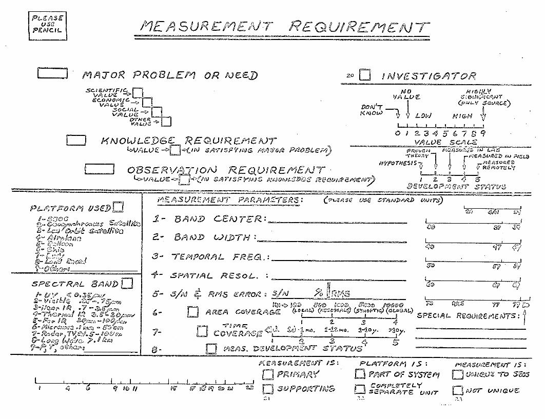
meteorological observables. Measurement Requirement sheets such as the sample

attached will be filled out and the information transferred to punched cards

and computer correlated and classified to develop a consistent set of technical

P.NCIL

M a iOR PROB LEM1 oR Ai) FSF Fo- i vriZo0 Li OA1VES-r1C7A7OR

sc- 6Ar'IF/C.

vP&ALC - m Kova L SE REp'IREM EAJ

Z O SENR/jLIO) r fEQL Eu E IPE/D~eR~ylP / EeIErBEpdTo

C> ~kei-A LoC:J-<,Qs S *SE~JJ c, Sir' msS D ak n F,!sf>Edpa;ba~~w

NOIVA L. E_

wsw V LOW

.peCS LrC. T°-OL- SCRC.)

HIGHI I I~ sI iJ I

VALOE SCAL_

p v J g REJR o77L''R ~~~ " .-- n -R- XT~RWOTNC~SIS79 IqCA506ED

I 2.> > ea -3 o< 5~ib

. Al64ce 2

0- LD5~'cR'~2o'~ ~i

SDLd-A&sDJ iSPE c-RAL SAASILi- Uv < gao -P- vor XG-foo

~-oc rse ws·l. DO~3-n.9-VAQSp 1A1 .7° >Sr9

r C,=

o,

.-- T- -

r~~~s P,~9 CAWT&/?S:6~

1- aAND CEAJ)TE,:

3- 'tEPaPoRA/L FE6L,:

4- SPPA/AL RESoZL.

5- 5/5 4 R'igs EZO,

7-

'&'AS' UJSE SD'AJA)Zar VV/7~);,'

II ~I --co SY 10N

S/ 162. -;J .lNI

1 2. 3 45 3o <a .? I .M. B.¢. ° ,-D y.

Li mCza. STA7-u'Q UL6:-= $4

i I4m 47 .'-

I- i _

I , .L. .

SPECIAL REQLV2ZEplF)T$S:

A vl Su2 0- CNO /S:

I , I - -i [.3] Pr, -,HA- AI , I, . I I: .I:^1:

[] 6CPP1 'r / 5:LX PRP A o o ns ,

C t::Pa1PL'5C7ZsEp pOItI PL'i/

.

PI-ASV.2zewr /5:

2 A3 > vaoJuGr

//EA SUREEi/7VT REG u/REE rAy-- %-

L I I I , I

_ __--_·--111 __ _��_·____

U _.-__

. B . = . . . ... . . .

1��-11 -~---�-�---�-�

�---�--

V, m -, laz) 0-0 oco Oc -5 (gpd

AREA G"UAI -)nL :CQe~ ugpoa (DLILt 9 Te - -

I- � I- -

-- �I · YIIIII----·-XII�-- _ I � I- _- LA:=LL 7 7 c �

I

?-- 0akt bD wo-rH· :

17

requirements which is complete for the phenomena we have investigated.

If time permits, the study will be broadened to other mesoscale phenomena

and potential uses of SEOS in order to make a more complete survey. For the

present, we are concentrating on analyzing and documenting the unique and

significant contributions of the seminar. A full description of the study

results will be completed before the next quarterly report.

Conclusions and Recommendations

None at this time.

APPENDIX

Part VI

"Boundary Layer Response and Asymptotic Stability"

1. Introduction:

In the following, the term "Boundary Layer Response" refers to the motion

of a flexible satellite near the time t = 0, and is not to be confused with the

response of the atmosphere.

In the earlier phases of this work, it was seen that the response of the

system near the time t = 0 was found to be given essentially by the outer

boundary layer equations (3.70) and (3.71). These are rewritten here as follows:

A(_B,0)Y(wB,T) + / B(wB,O)( WB,T) + y(_BT) = 0 (3.70; 6.1)

[AVy]( _lB,0) t (T) + 2 [AVl](WB,0) (T)--1 -'-

+ V[A+y](wB,0 ) wl = d(B' ) (3.71; 6.2)

It was also seen that the long time response of the system is basically

governed by Eqs. (5.58) and (5.113). These equations are

(5.58; 6.3)· B x + B k + B x = 0I- 2- 2- 3-

. A aq + A 0 + A = A20 30 ° -0

(5.113; 6.4)

Equations (6.1) and (6.2) will now be considered in detail for the

boundary layer response. Then Eqs. (6.1) through (6.4) will be examined for

stability of the satellite motion. The notation in these equations were

defined before.

2. The Boundary Layer Equations

The functional matrices A and B of Eqs. (6.1) and (6.2) are defined in

Eqs. (3.6) and (3.7). In Eqs. (6.1) and (6.2) these matrices are to be

and

2

evaluated at t = O. This makes these two linear second order equations

with constant coefficients. Hence y(T) is given by

y(T) = 3y(0O) + 4)y(O)(6.5)

where 4 and 4 are fundamental matrices of Eq. (6.1). Thus y(T)3 4

undergoes damped oscillations. For the two bodies A and B, Eq. (6.5)

becomes

-A3 A3 MA3(0) + 3 A4 -A3(0)

--3 = *B3 -M 3 (0) + +B 4 B3(0)

(6.6)

(6.7)

Substituting the forms of M andinto Eqs (6.6) -And (6.7), respectively,3

into Eqs. (6.6) and (6.7), respectively,

M-3 from Eqs. (4.21) and (4.23)

we obtain

SAl-B + SAiA + 2SA1lB + SA2 + SA3 + SA57BA2

- * [.iB ( {+ (--w + SA1(rb-S A5 6 A2B] + ABIA - 6A[IA] + S A(B

+B + SA2 B + SA4 + SA5 B A2B - SA5[ 6A2-_B]B

+6A BIAWB -6 A[IAB]B ] + SBA2_B

+[SAs 6 A2 + 6AIA + S A5A 2 B-

A5 [B-] A2- A A B- A B- A-

+ +SA5 [B-]A2 Br-~ + 6A[B-A]IB ABe

+ SA5F B6A2-B +A BIA-B 6AuA

=A MA3 (O) + A4-AA3( 0 )(6.8)

3

20and

S WB1-B +sB2- + B3-B + sB4- + sB5 B B2-B

+B B B-B 6B-B =B3-B3(3) + B4-B3( ) (6.9)

From Eq. (6.9), 0 is solved in terms of -B' and we obtain

= exp[-SBSB4t] 0 +f exp[SB2SBT] [g(T)

+ BMB3(0 ) + ~B4-Bf3(0) (6.10)

Eliminating 0, 0 and 0 from Eq. (6.8) by using Eqs. (6.9) and (6.10), the

boundary layer equation for _rB, corresponding to Eq. (4.6a) is obtained as

t

1-B 2-B 3B2B + BB + B4 B5(Tt) [ BUB

*

-S. _B - SB ] (T)dT d + B6u B + B B - A u

+E f(sB '-B ',--uA'-UB) B(t) (6.11)

where.

B (t) [-O S-B2 B3(t) + (SA2+SA3)S-1 B(t)] -3 (O)B8(t) 4 -BAF(t)~ - A1 B2 B3 -MB2(o)

[SAlB 21B(t + (SA2+SA3)SB2B4( ]-B3(0)-t)

-SA4 B5 (T-t) [+ ¢Bi)B 3(T)MB3(0) + B(T)MB3(0)] d

+"A (t)MA3(0) + pA4(t)'-A 3(0) (6.12)

As the body B is nominally static, the terms involving the products of

uB or- B with MB3(t) have been neglected in deriving Eq. (6.11).

4

3. Boundary Layer Solution for B

The maximal probabilistic boundary layer solution for _B is obtained in

a way similar to that used for the asymptotic case. Corresponding to Eqs.

(5.44) and (5.45), the governing equations in this case become

T.. T TBA -B + BX +g (6.13)1-1 2-1 3-2-

and it

B w +B + + B3w B B +S ei(T3d41-B 2 + B 3B B4 Bl-B B3-B

t 0

+(t) - Bs(t) = s¢ g3(tlT)A (T)dT + gA 1+ g ] (6.14)

Comparing Eqs. (6.13) and (6.14) with Eqs. (5.44) and (5.45) we see that

the term B Fi of Eq. (5.45) has been replaced by -B (t) in Eq. (6.14)

without any other change. Hence all the expressions for -B' derived for the

asymptotic case becomes applicable to the boundary layer case if -B (t) is

substituted for B F 04 1-

4. Boundary Layer Solution for w-1

The governing equation for the boundary layer solution for w is given--1

by Eq. (6.2). As the coefficients of w1' 1 and x1 are evaluated at

t = 0, the equation is one with constant coefficients. The initial conditions

are lumped on Eq. (6.1) and so w has zero initial conditions. Hence the--1

solution wl for the bodies A and B are given respectively by the Duhamel's

integrals as

t

-A 5 ( -BO (6.15)--A ~+S(-~(-B0)d

5

and t rU-W

-B1 J B5 (t-T)d(B, O)dT. (6.16)

In the above two equations, ~A5 and B5 are the appropriate fundamental

matrices of the homogeneous equations of Eq. (6.2) for the bodies A and B,

respectively.

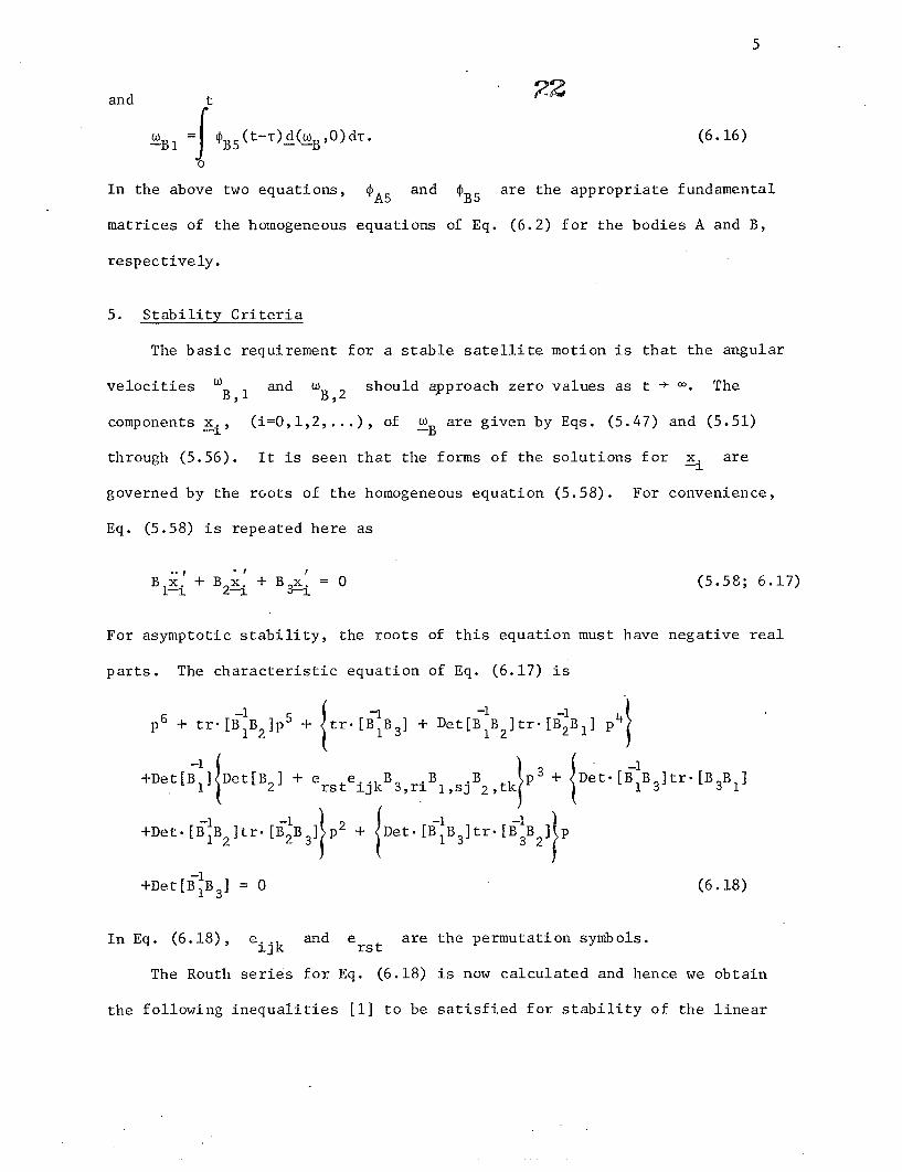
5. Stability Criteria

The basic requirement for a stable satellite motion is that the angular

velocities W and wB should approach zero values as t + a. TheB,1 B,2

components x., (i=0,1,2,...), of __B are given by Eqs. (5.47) and (5.51)

through (5.56). It is seen that the forms of the solutions for x. are--1

governed by the roots of the homogeneous equation (5.58). For convenience,

Eq. (5.58) is repeated here as

Bx + Bx + Bx = (5.58; 6.17)1--i 2-i 3-i

For asymptotic stability, the roots of this equation must have negative real

parts. The characteristic equation of Eq. (6.17) is

-1 5 -1 -1 -1p6 + tr + t[B B3 ] + Det[B 1B2]tr.[B2B1] p4

rDe[B et[ + p3 + Det.[B1B3]tr.[B3B1]+Det[B1] 2] + erst ijk 3,ri lsj 2 ,tk 1 3 3

+Det-.B ]tr.[Btr B3 ]2 p2 + tDet-[B1B 3]tr.[B3B ]2p

+Det[BB 3] = 0 (6.18)

In Eq. (6.18), eijk and erst are the permutation symbols.

The Routh series for Eq. (6.18) is now calculated and hence we obtain

the following inequalities [1] to be satisfied for stability of the linear

6

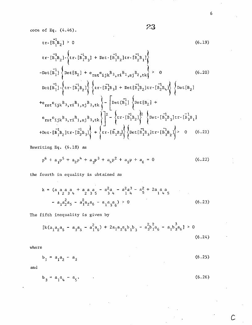
core of Eq. (4.46).

-1tr.[B1B2] > 0

-1tr' [BB2].tr.[BB] + Det[B1B2 ]tr[B2B],tk

-Det[B1 ] {Det[B2 ] + ersteijkB3,riBl,sjB2,tk I

A

0

Det[B].{tr [BIB 2] {tr.[BB 3] + Det[B1B2 ]tr.[B2B4] Det[B2]

-ersteijkB3,riBlsjB3,tk - Det(Bl] {Det[B 2] +

rst ijkB 3,riBl,sj 3,tk 3t r [BB2 ]

B tDet.[BB2] 3] tr.[B] 0-Det.[iB12]t.[2B3 ] -tr[~B ] Det[B11B3] tr.[ 3B2] > 0 (

(6.19)

6.20)

6.21)

Rewriting Eq. (6.18) as

p6 + alP + a2p4 + a3p3 + a4p 2 + ap +a= 0

the fourth in equality is obtained as

k = (a a a a + a a a - a2a - a2a 3 - a2 + 2a a a1 2 3 4 2 3 5 3 4 1 4 5 1 4 5

2 2-a 1a 2 a 5 - ala2 a 6 - ala3a) >0

(6.22)

(6.23)

The fifth inequality is given by

2 22 3[k(a1 a2 a5 - a3a5 - ala 6 ) + 2ala 3a 6blb 3 a3ba 6 ab 3 a >

(6.24)

where

and

(6.25)bi = ala2 - a3

b= a a - a .3 1 4 5

(6.26)

C

((

A

7

The last inequality to be satisfied is

a6 = Det.[BIB3] > 0 (6.27)

The above inequalities will all be obviously satisfied in a well-designed

satellite. These also yield a comparison technique for two satellites. The

comparison is to be made on marginal stability. The design for which al and

a6 are larger has a larger marginal stability and hence is the more desirable

one.

We now consider Eq. (4.25) to examine the conditions for stability of the

relative rotation, O. Equation (4.25) is repeated here for ease of reference.

0 = exp - SB2SB t e + expSBSB4 (T-1 g(T)d (4.25; 6.28)

where g(T) is defined by Eq. (4.26). Evidently, the primary requirement for

-1

stability of 6 is that the eigenvalues of the matrix [-SB2SB4j must have

non-positive real parts. There is another interesting requirement on these

eigenvalues. This arises due to the appearance of g(T) in the integrand in

Eq. (6.28). This requirement is obtained in the following discussion.

-1Let -11,' -P2 and -P3 be the real parts of the eigenvalues of [-SB2SB4],

such that

IP11 > IP21 > IP31 (6.29)

Let -al'- 2 ,'-o 3 be the real parts of the eigenvalues of Eq. (6.17), such that

111 > 1a21 > 131 (6.30)

Then from Eq. (6.28), we have

P3 t ie elT -P 3t -C3 T

0 < e + a . e e e dTr

o

8

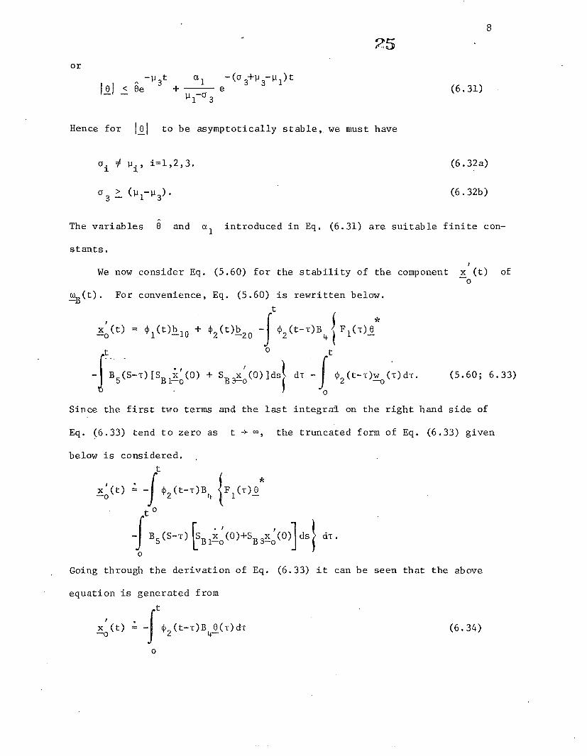
25or

^ -P3t a1 -(oa 3+ 3-Pl )tJ < e +- e (6.31)

11-03

Hence for 181 to be asymptotically stable, we must have

pi' =1,2,3. (6.32a)

0 3 (1 -P3). (6.32b)

The variables 6 and al introduced in Eq. (6.31) are suitable finite con-

stants.

We now consider Eq. (5.60) for the stability of the component x (t) ofo

_.B(t). For convenience, Eq. (5.60) is rewritten below.t

(t) = 1(t)bl0 + 42 2()b2 0 - (t-T)B F()

- B(S-T)[S Bo() + SB (O)]ds dT - (t-T)w (t)dT. (5.60; 6.33)IB IKo B t2Since the first two terms and the last integral on the right hand side of

Eq. (6.33) tend to zero as t + A, the truncated form of Eq. (6.33) given

below is considered.

t

x-(t) | 2(t-T)B F((T)3

-o

Going through the derivation of Eq. (6.33) it can be seen that the above

equation is generated from

t

x (t) 2 (t-T)B 0(T)dT (6.34)-o

9

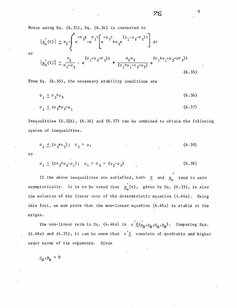
Hence using Eq. (6.31), Eq. (6.34) is converted to

a I -a t aT (

03 3t L *e 3T+ 3eo

or

() < a2 (a -1 3 3 )t a 2a 3 ( 1+p1 1-p 3-2a 3 )ti _,(t)I < e + (a +Pa e

-o -a 1 -p 3 (l+Pl-a 3- 3)

(6.35)

From Eq. (6.35), the necessary stability conditions are

al < a3+p3 (6.36)

a 1 < 2a 3+P3-P1 (6.37)

Inequalities (6.32b), (6.36) and (6.37) can be combined to obtain the following

system of inequalities.

a .< (a 3+p 3 ); a 3 > P, (6.38)

or

a 1 < (2a03 +P 3-Pl); P > a3 > (P-P39)

If the above inequalities are satisfied, both 0 and x tend to zero

asymptotically. It is to be noted that x (t), given by Eq. (6.33), is also--o

the solution of the linear core of the deterministic equation (4.46a). Using

this fact, we now prove that the non-linear equation (4.46a) is stable at the

origin.

The non-linear term in Eq. (4.46a) is c f(-B,`BUAUB). Comparing Eqs.

(4.46a) and (4.35), it can be seen that c f consists of quadratic and higher

order terms of its arguments. Since

UA'UB 0

10

if

--B'B + 0 ,

we have

Lim cIf (v) -Lim = 0

Ivl

-B

v = [_B'-B'-,A'

(6.40)

Then from the Theorem 1, of Struble [2], and the non-linearity condition

(6.40), it follows that Eq. (4.46a) is stable at v(t) = 0.

We now analyze the behaviour of the stochastic differential equations

(5.44) and (5.45). These non-linear equations are

BXl - B + BT3A = c gi+g2Xi1i 2 3 1 1 21 I1 (5.44; 6.41)

Lt JB& +Bw +B w -B JB 5 (r-t)(S c)+S d-c1-B 2-B 2B 3B 4 B-B+B3B)()d

t 0

+w(t) + B4 F 1- = [ g 3 (tT)Xl(0)dT + g4A_ + g511 - f (5.45; 6.42)

It can be proved that the eigenvalues of Eq. (6.17) and those of the left hand

side of Eq. (6.41) are equal in magnitude but opposite in sign. Thus A1 is

unbounded. This result is expected as A , which is a measure of the indeter---1

minacy of the value of -B' should grow larger with time. An interesting

point to be noted is that the larger the marginal stability of WB' the larger

is the marginal instability of -X. Equation (6.42) is now considered to

resolve this apparent paradox.

11

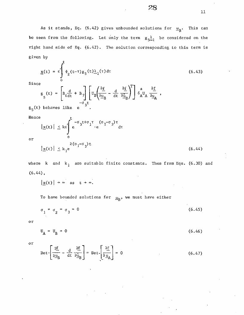
As it stands, Eq. (6.42) gives unbounded solutions for wB. This can

be seen from the following. Let only the term g5X1 be considered on the

right hand side of Eq. (6.42). The solution corresponding to this term is

given by

Since

t

x(t) = E 2 (t) 2 (t- T )g 5 ( t ) l( T) d

0

IB-aId -afg (t) = d + B -

6dt B dt -

g5 g) Denaves liKe e

us PA-

(6.43)

* af

AUA au--A

t

Ix(t0l < -e 3t+ a1T ( 1-o 3) T

2 (a 1- C3 ) tIx(t)I < kIe (6.44)

where k and kl are suitable finite constants. Thus from Eqs. (6.30) and

(6.44),

Ix(t)l + - as t + a.

To have bounded solutions for wB, we must have either

r 1 02 =3 =0 (6.45)

or

(6.46)UA = UB =0

or

[_f d fDet.- = Det = 0

dt uB dt I Det.-, =0ALB u.B Pu

-nenice

or

(6.47)

- / - N

dT

2 9 12

The condition (6.45) ensures purely oscillatory motion of the satellite and

is too restrictive. The condition (6.46) implies deterministic forcing and

control torques. This also is quite difficult to achieve. The implications

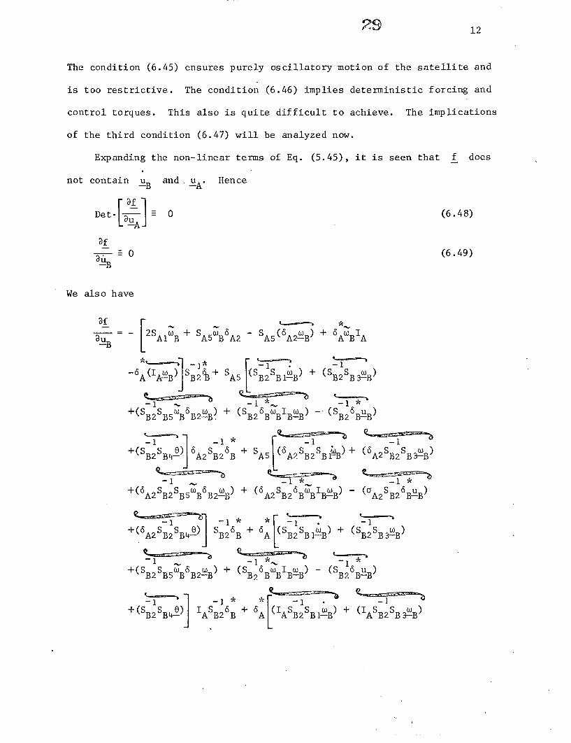
of the third condition (6.47) will be analyzed now.

Expanding the non-linear terms of Eq. (5.45), it is seen that f does

not contain uB and uA. Hence-B -A

Det. L- 0 (6.48)

afE 0 (6.49)

aB

We also have

au 2SAB + SA5 B6A2 SA5(6A 2_B) + 6AaBIA

---] -i -1 -1

-6A(IA!B)]SB2B+ SASB 2SBiL-B) + (SB2SB 3BB)

-1 -1* -1 *

+(SB2SB5 B B2_B) + (SB26I ) - (SB2B-B)

-1 -1* -1*( B2 B4-)S A A2 B2 B A5 A2 B2 B1-PB) (6A2 B2 B3-B

+(6A2SB2SB5WB6B2_B ) +(6A2SB26BBI B BB)- (GA2SB26B-B)

+(6A2SB2SB40) SB26B + 6A SB2SB1-B) B2 -B

-1 -1

+(SB2SB)B B22B) + (s 2IB B1B) +- ( IASB2SB3

+(SB2SB00) j IASB26 B +

30 13

1 -1 * -*

A B2 B5 B B2-4) + (IAB2 OBIB-4) (IA B2 B-B

+(IASB2SB) SB26B - SA5(6A2B)SB26B - SA5( B)A2 SB2 B

· -' -1 * *-- - 1 *--A(IA B )SB2B - A ( AB26B (6.50)

From the above equation, it is seen that Eq. (6.47) can be satisfied if

DetS 6B= 0 (6.51)

Since Eq. (6.51) can never be satisfied, it seem that the random torques tend

to increase the variances of -B indefinitely though the mean values of -B

decrease asymptotically.

6. Single Composite Body Analysis

a) Equation of motion

We now modify the previous analysis for a satellite which consists of the

body B only. This satellite may either be a spin stabilized or a three-axes

stabilized one. All equations through Eq. (4.3) remain valid. Since there

are no contact forces and torques for a single body, equations corresponding

to Eqs. (4.4) and (4.5) become

A = [6B1]B + [6B2] B (6.52)

P = uB - [I B]B + [hB] B - B[I B]B (6.53)

Then the equation for 0B' corresponding to Eq. (4.23) is

S Bi-B + SB + SB5wB[6B2] B

+[B = 0 (6.54)*+[c B ]WB [IB]WB [- 6B]uB = 0 (6.54)

d3I 14

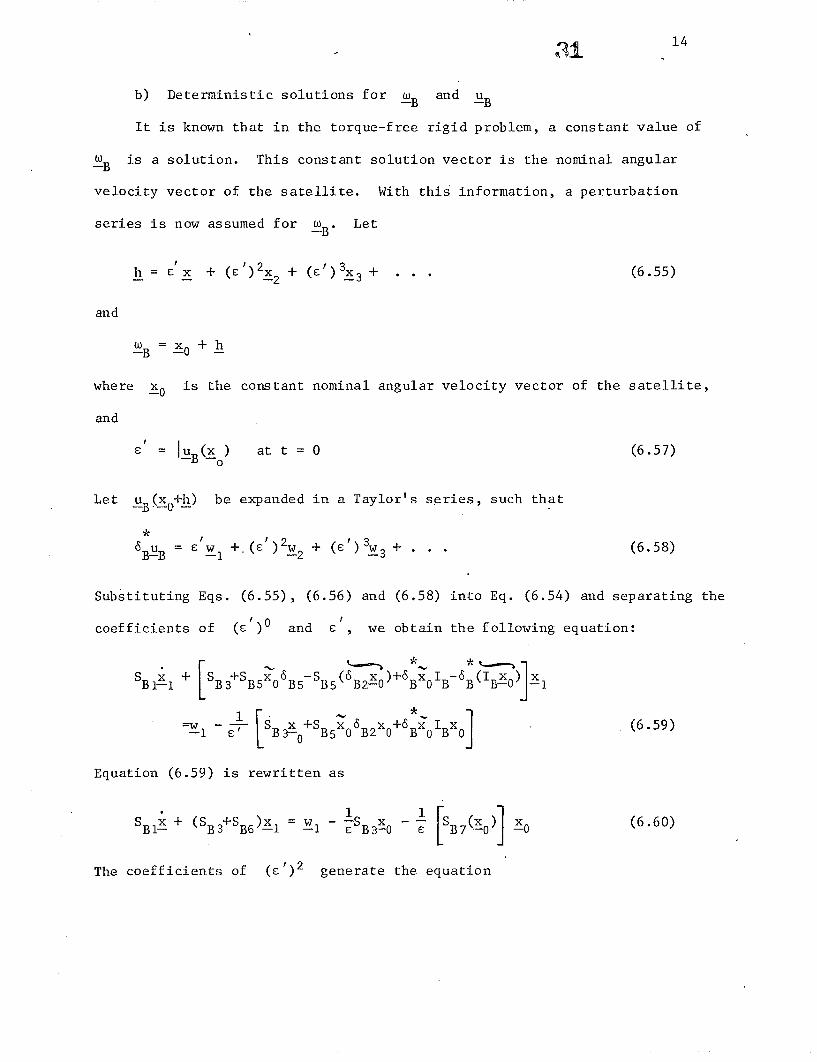
b) Deterministic solutions for wB and UB

It is known that in the torque-free rigid problem, a constant value of

LB is a solution. This constant solution vector is the nominal angular--B

velocity vector of the satellite. With this information, a perturbation

series is now assumed for wB. Let

h = x + () + ( ')3 x3 + . .. (6.55)

and

- x + h-B -O

where xO is the constant nominal angular velocity vector of the satellite,

and

IUB (X ) at t = 0 (6.57)

Let uB(xo+h) be expanded in a Taylor's series, such that

6BB = w 1 + (E') 2w 2 + (') 3 w3 +. (6.58)

Substituting Eqs. (6.55), (6.56) and (6.58) into Eq. (6.54) and separating the

coefficients of (C )O and c , we obtain the following equation:

s x +Is +s £6 S IIB-_ [ B3 B5 06B5 B-S ( B2-0) B +6xTB- B( 0)- x

1 s [ B B B2 BX B(6.59)--w--1 -' %SB5 0B2X0+6B

Equation (6.59) is rewritten as

(S )x 1 x (6.60)SB1 + (SB3+SB6)Xl Wl - SSB B7- -O (6.60)x0

The coefficients of (e')2 generate the equation

15

SBll (SB3+SB6) = -2 SB7(l] - (6.61)

From the coefficients of (¢C)3, we obtain

SBlX3 + (SB3+SB)X3 = 3 -2 [SB7 (x)] xl (6.62)

Equations from higher powers of E can be obtained similarly. Equations

thus obtained are linear with constant coefficients and will be solved as

shown in the earlier parts of this work.

Since the control torque functions w. appear linearly in Eqs. (6.60),

(6.61) etc., w. can be shown to be a "band-bang" control by the method--1

shown earlier. Thus the controls for a single body satellite are seen to be

much simpler than those of the dual-spin configuration.

c) Random solutions for -B and uB

We now follow the method outlined in Part 5 of this work to obtain the

statistical parameters of the random torque responses. The functional, J,

to be minimized in this case is given by

J = [(0) - B(0)] RO [B(0) 7-B()]

+i Zl(t)-ZR(t] R t1 (t)_ZI(t

I - - I -

UB(t) -uB(t)I UB (t)[u-B(t) jB()

+2 _Bl B+SB 3 SB5wB6B2wB + WBIBB

6B-BB + 2[ B dt + 2X4(z 1-h1) (6.63)

For J to be minimum, the following set of equations are to be solved simulta-

neously:

16

SBlB + SB3B + SB56B2_B 2- B B B-B -6B (6.54)

z (t) h[IB(O),t] (6.64)

uB) = (t) + UB(t)+ UB[B] (6.65)

wB (0) = _B(0) + RO [SBl)(6.66)-B 131 (0)+X](6.66)

uB(t) = UB(t) + UB(t)_2 (6.67)

z1(t) = zl(t) + Rl(t)_A4 (6.68)

B1-1 -2 BT B B2-B- BB B.BB1iTSBlTl SB3 + (B SB +B6B2-B+BB B-B)] l

( ·-B \ T=-- ) T (6.69)

A (T) = 0 (6.69a)--1

These equations are reduced to

· *S W + w + w WB -B+ SB3B + SB5wB2-B + 'B BI-B

=*6B (6.70)

B[(t)+UB(6 B) (t (670)

and

T *T

BS1- S 3+ 5 wB B2-SB5( B2-B) BB B w B -B(IB-B -sB - S B3B5%BB2BS(6 w )+6BcBI -6(I _~] 1 = 0 (6.71)

To solve Eqs. (6.70) and (6.71) the following series are used:

B 0 X + x + (E -x + ()3X + . (6.72)

1 : A £10 + C(' 1 + () 2 A + (E') 3 A + . (6.73)1 10 11 -12 -13

--: = '- + w + ( 3 + .. (6.74)6B U.B 1 w -3

17

Let U be defined by

J * *

sU= 6BUB6B (6.75)

Then from Eqs. (6.70) and (6.71) the following set of equations are obtained:

T · TSBl1O - (SB3+SB6) lo = 0 (6.76)

SB (SB3 S 6 )X 1 - -S B73Xo)] Xo UX (6.77)

T TB- B3 B6 -11 SBSB6)7( ) (6.78)B 1~---11

SBl2 + (SB3+SB6)x2 =w 2 [SB7(X x1 + UX11 (6.79)

T TS - (S(6.80)B1-12 (SB3+SB6) 12 [SB7 (-x2] -- lo B7 (6.80)

S + (S + )x w L B7 J -2 L (7x2'i2 1 + UX (6.81)SBi--x3 + (SB3+SB6)x3 = w3 - [SB7T(xl -2 - LB7(x2 x-1 -12

Similarly, more equations of this sequence will be obtained. It is evident

that the random solutions coincide with the deterministic solutions if

UB = 0. These equations also will be solved by the method outlined in Part

5.

From this, the mean and the variances of the pointing error of any rigid

body will be obtained as shown in Part 5.

d) Stability criteria

As in the case of the dual-spin configuration, the random parameter A--1

is unbounded, if the mean values of the response are maintained stable. This

also implies that the variances increase indefinitely. We now obtain the

criteria for stability of the mean values of !B'

18

From Eqs. (6.77), (6.79) and (6.81), it is clear that the asymptotic

stability is governed by the roots of

SB1x + (SB3+SB6)x = (6.82)

For a stable solution, the roots of Eq. (6.82) must have negative real parts.

The characteristic equation of Eq. (6.82) is

Det.[SB1]. p3 + Det [SBJ.trISB (SB3+sB6] p22

F p+Det .B B1 3+SBF =+Det SB3 SB6] tr (SB3+SB6 SBp + Det SB +SB 6 = 0 (6.83)

Using the Routh series of Eq. (6.83), the following inequalities are obtained

as the required criteria:

Det [SB!] > (6.84)

Det [SB 3+SB6] >0 (6.85)

tr. LB (SB3+SB] > 0 (6.86)

and

tr.[SB(SB3+SB6 )] tr.[(SB3+SB6)-SB] > 1 (6.87)

7. Performance Criteria of Satellites

Based on the preceding analysis we now propose several criteria for

evaluating the performance of satellites of different designs. It has been

shown that for each satellite there is an associated outer boundary layer.

The duration of this boundary layer depends on the structural properties and

the nominal angular velocities of the satellites. This duration is /,

where Eq. (3.5) defines c as

19

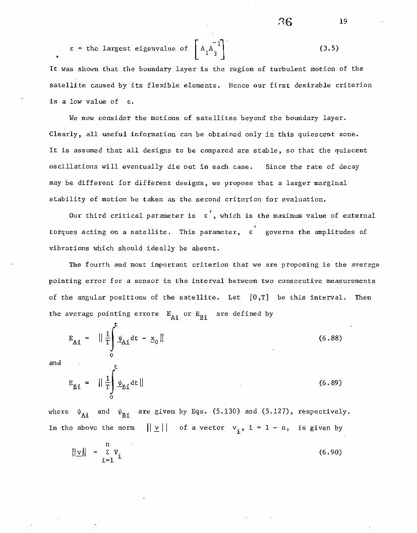
£ = the largest eigenvalue of A 1A (3.5)

It was shown that the boundary layer is the region of turbulent motion of the

satellite caused by its flexible elements. Hence our first desirable criterion

is a low value of s.

We now consider the motions of satellites beyond the boundary layer.

Clearly, all useful information can be obtained only in this quiescent zone.

It is assumed that all designs to be compared are stable, so that the quiscent

oscillations will eventually die out in each case. Since the rate of decay

may be different for different design's, we propose that a larger marginal

stability of motion be taken as the second criterion for evaluation.

Our third critical parameter is C , which is the maximum value of external

torques acting on a satellite. This parameter, C governs the amplitudes of

vibrations which should ideally be absent.

The fourth and most important criterion that we are proposing is the average

pointing error for a sensor in the interval between two consecutive measurements

of the angular positions of the satellite. Let [0,T] be this interval. Then

the average pointing errors EAi or EBi are defined by

t

EAi II 1 idt x (6.88)

and

EBi || dt| (6.89)

o

where Ai and ~Bi are given by Eqs. (5.130) and (5.127), respectively.

In the above the norm |I vi of a vector vi, i =1 - n, is given by

n

IIvll = z V (6.90)i=l1

7 20

8. Conclusions

We now have come to the end of our analysis. In this analysis, the method

of obtaining the motion of the sensors aboard a satellite is obtained by per-

turbation techniques. The most probable motion is obtained after considering

random torques, initial conditions and measurement errors. Several stability

criteria have also been established. Finally, several performance evaluation

parameters have been proposed. It is hoped that these parameters will be a

useful tool in comparing the pointing accuracy of different satellites.

Numerical results will be presented in the following parts of this work.