Control of unicycle mobile robots

Citation for published version (APA):Geluk, T., & Bommer, A. (2003). Control of unicycle mobile robots: Bellybot & Trilobot. (DCT rapporten; Vol.2003.118). Technische Universiteit Eindhoven.

Document status and date:Published: 01/01/2003

Document Version:Publisher’s PDF, also known as Version of Record (includes final page, issue and volume numbers)

Please check the document version of this publication:

• A submitted manuscript is the version of the article upon submission and before peer-review. There can beimportant differences between the submitted version and the official published version of record. Peopleinterested in the research are advised to contact the author for the final version of the publication, or visit theDOI to the publisher's website.• The final author version and the galley proof are versions of the publication after peer review.• The final published version features the final layout of the paper including the volume, issue and pagenumbers.Link to publication

General rightsCopyright and moral rights for the publications made accessible in the public portal are retained by the authors and/or other copyright ownersand it is a condition of accessing publications that users recognise and abide by the legal requirements associated with these rights.

• Users may download and print one copy of any publication from the public portal for the purpose of private study or research. • You may not further distribute the material or use it for any profit-making activity or commercial gain • You may freely distribute the URL identifying the publication in the public portal.

If the publication is distributed under the terms of Article 25fa of the Dutch Copyright Act, indicated by the “Taverne” license above, pleasefollow below link for the End User Agreement:www.tue.nl/taverne

Take down policyIf you believe that this document breaches copyright please contact us at:openaccess@tue.nlproviding details and we will investigate your claim.

Download date: 29. Dec. 2021

Control of unicycle mobile robots: Bellybot & Trilobot

Theo Geluk 480735 Ard Bommer 472173

Supervisor: Prof. Dr. Henk Nijmeijer

Coach: Dr. ir. Paul Lambrechts

Contents

1 Introduction ...................................................................................................... 3 2 A unicycle mobile robot ................................................................................ 4

2.1 Dynamics ....................................................................................................... 4 . . .............................................................................. 2.2 Denvation of an observer 6 .................................................................................... 2.3 Trajectory generation 6

................................................................................................. 2.4 Use of a filter 9 3 Trilobot ............................................................................................................. 12

................................................................................................. 3.1 Introduction 1 2 ................................................ ............................ 3.2 Q-basic programming .. 1 3

..................................................................... 3.3 Tracking cslltroller in Matlab 1 5 ......................................................... 3.4 Using another way of communication 17

4 Bellybot ............................................................................................................. 19 .................................................................................................. 4.1 Introduction 19

.................................................................. 4.2 A mouse as trajectory generator 19 ....................................................................... 4.3 Experiment 1 : Mouse-signal 2 0

................................................. 4.4 Experiment 2: Mouse as input for Bellybot 21 ..................................................................................................... 4.3 Problems -23

.......................................................... 5 Comparing Trilobot and Bellybot 25 6 Conclusions and Recommendations ....................................................... 26 Appendix I Simulink implementation of unwrap system ................ 27

........................... Appendix I1 Simulink implementation of the filter 28 .............................. Appendix I11 Q-basic script of tracking controller 29 .............................. Appendix IV Matlab script of tracking controller 31

... Appendix V Simulink implementation of a trajectory generator 33 Appendix VI Files ............................................................................................ 34

1 Introduction

'Control engineers must master computer and software technologies to be able to build the systems of the future, and software engineers need to use control concepts to master the ever-increasing complexity of computing systems.'[5]

To control a modern mobile robot a control engineer does not have to master control techniques only, also knowledge of software technology and electronic technology is required. A system where multiple of those technologies are integrated is called an embedded system. hi embedded sysiems cei~trel teckiqvles zre used, which xc mostly well documented and repeatedly re-used. When software is involved in a system, problems may arise because software technologies are changing all the time. Also for one problem mostly muitipie software solutions exist. Tnerefore a control engineer should not only document the control techniques used, but also the software techniques. To direct and control mobile robots one should use a combination of those techniques that are well geared to one another. This implies that one should reckon with the dPxnics of the mobile robot, the electronics, which drive it and are used in the measurements. Also the software that enables communication with and control of the robot should be taken into account. Another important part is the trajectory or path that the robot has to follow. Information about the trajectory is needed. Herein there is a difference between an offline and online generated trajectory. In case of an offline determined trajectory, this trajectory can be converted into a suitable control signal for the robot. Concerning an online, real-time generated signal, problems can arise because there is not enough information about the trajectory in time. This implies that one is not sure that the robot is able to track the path in future time. Therefore an adjustment should be made to the reference signal that enables the robot to follow it in every case. The goal of this study is divided in 2 parts. The first goal is to make a mobile robot operational and the possibility of a tracking controller for an offline-generated trajectory is investigated. The second goal is to make an online-trajectory generation for a mobile robot. The organization of this report is as follows: in chapter 2 general dynamics of and trajectory generation for a unicycle mobile robot will be discussed. h chapter 3 a tracking controller is developed for a robot that has to track an offline-generated trajectory. In chapter 4 a real-time generated trajectory is made suitable to be tracked by a mobile robot.

2 A unicycle mobile robot

Unicycle mobile robots are all based on the same principle. They are driven by two separate controlled wheels at the back and are able to turn around their axis. This means that a unicycle mobile robot is not able to move sideways. The kinematic models for unicycle mobile robots are generally almost the same. When a robot has to track a certain trajectory a controller can be used. For this tracking, two things are needed: information about the position and orientation of the robot and information about the trajectory. Information about the robot is needed as fee6back for t5e co~koller. Nomzlly psitior: is measxred. The orientation of a robot can be determined by an observer. The information about the path the robot has to track is needed to determine the inputlcontrol signals for the robot.

2.1 Dynamics

In the report of Sander Noijen [2] a controller and observer are proposed. The kinematic model of a unicycle mobile robot is defined:

This model consists of three states, T = (x, y, 8), respectively denoting the horizontal position, the vertical position and the orientation of the mobile robot, and two inputs ii = (v, w), respectively denoting the forward velocity and the angular velocity.

We consider the problem of tracking a reference trajectory 2, = (x,, y, ,8,) by the reference system:

x, = v, - cos er yr = v, - sin 8,

8, = w,

Where v, and w, are the inputs generated by a trajectory generator. The error

dynamics are expressed in a moving fiame by choosing x, in the direction of v and

y, perpendicular to this direction, as depicted in figure 2.1

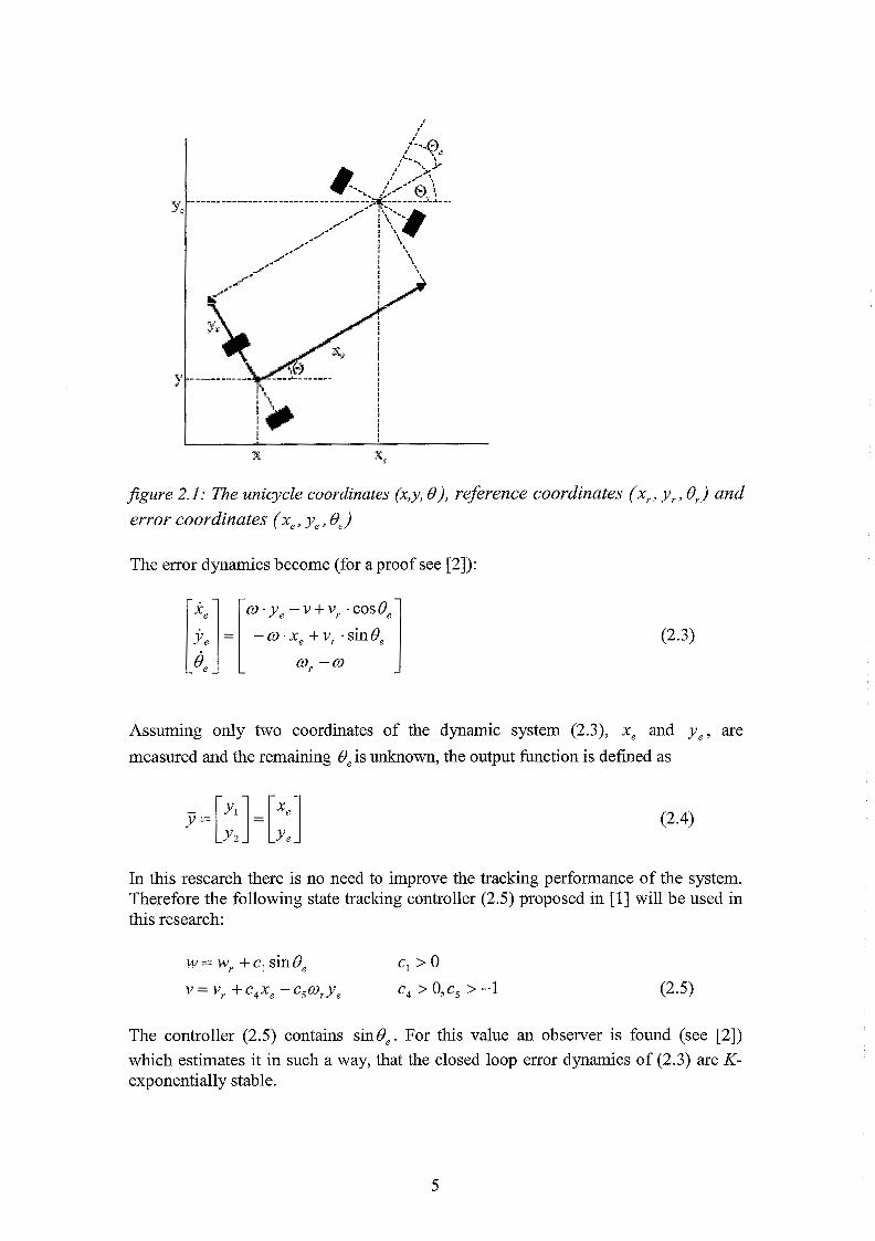
figure 2.1: The unicycle coordinates (x,y, B), reference coordinates (x , , y, , 8,) and error coordinates (x , , ye, Be)

The error dynamics become (for a proof see [2]):

Assuming only two coordinates of the dynamic system (2.3), xe and y e , are

measured and the remaining Be is unknown, the output function is defined as

In this research there is no need to improve the tracking performance of the system. Therefore the following state tracking controller (2.5) proposed in [I] will be used in this research:

w = w, + ci sin Qe c1 > O

V = V , + C 4 X e - C5 Wrye c, > 0, c5 > -1

The controller (2.5) contains sin&. For this value an observer is found (see [2]) which estimates it in such a way, that the closed loop error dynamics of (2.3) are K- exponentially stable.

2.2 Derivation of an observer

The observer-based controller (from [2]), which estimates the orientation of the robot, is dependent on the measurement of both the horizontal and vertical direction. The following help variables are used, each dependent on the measurement in x- or y- direction:

f = sine, + c2y,vr (2.6)

= cos e, + C3x,vr A A

With ( = sin 0, , yl = cos Q, and their estimates by = sin Be, @ = cos 0, , we define the

observer:

Defining the observer errors j = ( - J,@ = y - tp , with the controller of (2.5) and 2 c, = -4c2c6v, the 8, -dynamics become:

with v, bounded to satisfy the conditions for the existence and uniqueness of

solutions and v, persistently exciting (see [2]).

2.3 Trajectory generation

To direct a robot along a certain trajectory, information about that trajectory is needed. If a trajectory is presented as a path consisting of a number of points, then the only information available is the position of these points and possible the time elapsed between these points. This information should be converted into signals suitable for a mobile robot, like an orientation 8 , a forward velocity v and a rotational velocity w .

For computing v, the i - and y -component are needed. Tine desired orientation of the robot should be calculated, if the only trajectory information is the global position (x,y) of the points it consists of. This is possible using the derivatives of x en y, x - and y . With the orientation the values for w can be determined.

With use of the timestep At between two datapoints the velocity in the x- and y- direction can be determined with the following equation:

The velocity in the y-direction is calculated in the same way. The forward speed v then can be calculated by:

The desired orie~tation of the rob& is detemined with the s i p a d vahes of Itref and y,. With the signs of xref and yref the quadrant is determined. The

orientation Or%< can be calculated with the values of xref and yref , where is a help

variable to determine Bref .

Both, the quadrant and the orientation, are used to determine the orientation Oref by

adjusting the angle Oref (Bref = -Oref if in quadrant 4, or just Oref = Oref if in quadrant

1) or by adding n (if in quadrant 2, Bref = n - or by subtracting n (if in

quadrant 3, Oref = -n + Oref ).

Using (2.1 1) causes trouble when xref becomes zero, therefore the cases in which It,,.

or yref are zero Oref is determined without use of (2.11):

In the case of both iref and yref are zero, the previous orientation is retained until

= 0 = 0 > 0 < 0

iref or yref becomes a nonzero value. This implies that when the speed of the robot

becomes zero, it keeps the orientation during the last move. Through determination of 8 , as in table 2.1, Oref will never become exactly - n . Thus the orientation of the

robot will never become - n . For this orientation, where ir <O and yr =0, it follows

from table 2.1 that the orientation is n . This leads to an interval (- ir,n 1 of Bref .

Table 2.1

>O <O = o =O

The rotational velocity is determined by taking the derivative of Oref : wref = Oref .

n I2 -11712

0 n

When Bref switches from n to - n (or from - n to n ) in one timestep, because of the

2 z interval (- n , is I of Bref , it will cause a lugh peak (about - radlsec) in the rotational

At velocity wref . These peaks can cause problems, because they can force the robot to

turn in the wrong direction.

To get rid of these peaks the determination of wref has to be extended in such a way

that peaks in the wref -signai wiii be recognized and replaced by values that smootnen

the signal. Another possibility is to prevent Bref to switch from sign.

First an attempt is made to set a maximum siope for oref . If this siope is exceeded,

e.g. by 6 , switching from -n to n , the actual and calculated wref is replaced by

another value. This value is determined by adding the previous slope to the previous value of wref. Doing this, the slope in the wref -signal is kept.

x-position [m] time [s]

1.5

- 1 (0 a 2 0.5 - .,- P 0 cfr g -0.5

5 -1

-1.5 0 10 20 30 0 10 20 30

time [s] time [s]

4

From figure 2.2 its clear that Bref switches from n to - n (and from - n to n ). This

2a causes a peak (about - = 20n [radlsec]) in wref. In the omega-ref part of the figure

At

-- theta-ref 1

the blue line is the signal wref with eliminated peak values.

A second attempt is made to smoothen the signal wrgby using a filter which

eliminates all the signals with frequencies above 1 Hz. Using a filter causes a phase-

delay in the wTef -signal. Therefore the resulting wr# signal does not correspond with

the derivative of Bref on a specific moment, which implies that this filter is no option.

The third and best attempt is to prevent that Bref switches. The general idea is to add

k2x to Bref when it switches. If for example BEf switches from x to - x , 2 n is added

to Bref . This will cause BEf not to switch (figure 2.3). In Appendix I is shown how

this is implemented in Simulink.

theta-ref with adaption

T -, position / -- theta-ref without adaption 1

x-position [m] time [s]

-2 1 I I 0 10 20 30 0 10 20 30

time [s] time [s]

2 - omega-ref with adaption

Figure 2.3

Limitations of iref and yref have to be implemented, because a robot will have a

1

maximum values for v and w . It is preferable to avoid that the maximum values of v and w are exceeded. Ths is possible by use of a filter. This will be discussed further in section 2.4

- v-ref I

2.4 Use of a filter

I

If from a desired path the only available information is the x- and y-location, the orientation has to be determined. This can be done by use of a filter. This filter is used tr\ LV a dimate the values 2 mc! j , ~ E i c h c m be used to determine m estimate vahe fer

the desired orientation. The general relation between P,P and for a trajectory generator can be presented as:

The column U in (2.13) contains the external inputs, which are determined by the trajectory generator. w contains the model uncertainties. j is the estimated value of the position and ym,, is the measured value of the position. The value v is the measurement uncertainty. With U and w the dynamics of the trajectory generator can be approached.

The difference d = j - y m , should be minimized by the filter using the feedback gain

This gain has to be chosen in such a way that exponentially d + 0 for t -+ a. Its value is determined by use of the Kalman estimation function. This function is just used for tuning, the values for v and w are assumed to be constant. With tuning the

weighting parameters the output values, (i or ), are limited, which is needed to adhound the robot's input signals. The results of using a filter to process the trajectory data is shown in the following figure.

- POS with filter

x-position [m] time [s]

omega-ref with filter ---- v-ref with filter - 9.4

-s .' ; 0.2

-2 0 0 50 100 0 50 100

time [s] time [s]

From figure 2.4 its clear that the filter changes the desired path (and desired velocity) into a path the robot is able to follow. The forward velocity v can be bounded by use of the filter. For the rotational speed another solution is found, which is discussed in section 4.3. Implementation of this filter in Sirnulink and the determination of K is shown in Appendix II.

3 Trilobot

3.1 Introduction

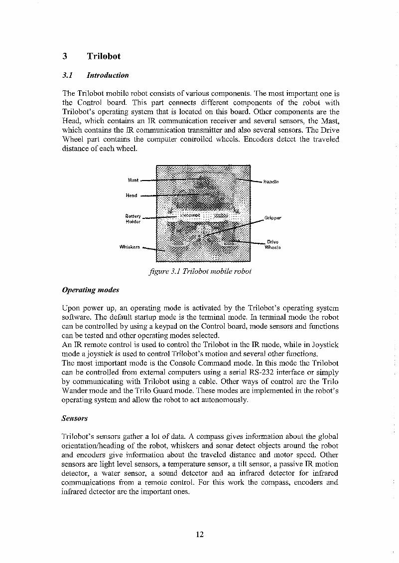
The Trilobot mobile robot consists of various components. The most important one is the Control board. This part connects different components of the robot with Trilobot's operating system that is located on this board. Other components are the Head, which contains an IR communication receiver and several sensors, the Mast, which contains the IR communication transmitter and also several sensors. The Drive -- d

Wneei part contains the computer eontroiled wheels. Zixode-rs deieet the traveled distance of each wheel.

&re 3.1 Trilobot mobile robot

Operating modes

Upon power up, an operating mode is activated by the Trilobot's operating system software. The default startup mode is the terminal mode. In terminal mode the robot can be controlled by using a keypad on the Control board, mode sensors and functions can be tested and other operating modes selected. An IR remote control is used to control the Trilobot in the IR mode, while in Joystick mode a joystick is used to control Trilobot's motion and several other functions. The most important mode is the Console Command mode. In this mode the Trilobot can be controlled from external computers using a serial RS-232 interface or simply by communicating with Trilobot using a cable. Other ways of control are the Trilo Wander mode and the Trilo Guard mode. These modes are implemented in the robot's operating system and allow the robot to act autonomously.

Sensors

Trilsbot's sensors gather a lot of d2t2. compass gives infomatition about the global orientatiodheading of the robot, whiskers and sonar detect objects around the robot and encoders give information about the traveled distance and motor speed. Other sensors are light level sensors, a temperature sensor, a tilt sensor, a passive IR motion detector, a water sensor, a sound detector and an infrared detector for inhared communications from a remote control. For this work the compass, encoders and infrared detector are the important ones.

When communicating with Trilobot by computer the RS-232 interface is used. With the Q-basic programming language commands can be send to and data requested from Trilobot. Also user defined control programs can be written in Q-basic enabling the user to control Trilobot by computer.

Compass

A digital compass is located on Trilobot's mast. Reason for this 'high' location is to minimize the interference of nearby objects that may disrupt the magnetic field. The accuracy of the conpass is 2 degrees 2:d cail be &ested by m u b y metd cbjects, magnetic Gelds or uneven surfaces. The compass returns values as a position code (North, South, etc) or the robot's heading in degrees with a resolution of 1 degree. Reading the compass takes approximately 0 2.5 sec.

Encoders

Trilobot is driven with 2 DC gear motors with optical encoder feedback. These motors can be controlled independently to move straight, rotate on center, or turn in an arc. To monitor the speed and position of the wheels the encoders are used. These encoders consist of a rotating wheel with 22 slots and an optical interrupter is used to- sense the slots.

Motor control

There are two ways to control Trilobot's motion: drive motor control and navigation control. Using drive motor control it is possible to determine the speed with which the Trilobot has to drive, the distance it has covered (in encoder counts) and the arc it has to turn (in a ratio code). For every drive motor control command send to Trilobot the robot returns an 'A', which indicates acknowledged. Using navigation control only rotate and move (distance) commands can be given. For velocity a default value, stored in Trilobot's operating system memory, is used. The difference with the drive motor control is the possibility to choose between commands whch return an 'A' when the motion has begun, or commands which return an 'A' when the motion command is completed. The first option prevents that there has to be waited for completion before a new command can be send.

3.2 Q-basic programming

With use of the Q-basic program language programs can be written to control Trilobot. Two kinds of commands can be send to Triiobot by the RS-232 interface, the get-cc-ad 22d the pI_lt-co~-rnand Get comands ask information from Trilobot, e.g. it's heading or speed. Put commands are commands Trilobot has to execute, e.g. move forward 15 feet.

A simple Q-basic 'tracking' controller

The encoders on the drive wheels give information about the position of the wheels, or the traveled distance. This information does not say anythmg about the global position of the robot, so the encoder data should not be used as feedback in a tracking

controller. A solution for this problem could be the determination of Trilobot's global position using the encoder data in combination with the compass data. By using position and heading, the 'global' position of the Trilobot can be calculated. A problem is that large errors may arise because of the low accuracy of encoder data and compass data. Because for each calculation of the global position the former results are used, the position error grows during Trilobot's motion.

Therefore the tracking controller is only based on the compass data. When the Trilobot is moving in a 'straight' line, a reference heading is set. With the compass . . dztiia, gmng infmmtion about Trilobot's actual heading, a check can be performed if Trilobot is still moving along the desired path. If Trilobot is diverging fiom that path commands can be send to Trilobot to get it back on track. In Q-basic this is all implemented in a loop. A move fcmmrd command (without waiting for completion) is send to the robot, this means that while moving forward, another (e.g. steering) command can be send to the robot. After the move forward command is send, compass data is requested from Trilobot to check the actual heading with the reference heading. If Trilobot diverges too much fiom it's reference heading, e.g. 3 or 4 demees, - a correcting steering command is given. Trilobot keeps steering until the desired heading is reached. Headed in the right orkriLat:loii, the move forward command is send again. Script of ths Q-basic controller is shown in Appendix 111.

To discuss results gained with this controller, data about the time that is required to send information (a command or a data request) to Trilobot and time needed for one loop in the controller is necessary. With this data it would be possible to determine the sample time or the rate with which the controller is able to update Trilobot's input signal. To process this information an implementation has to be made to store Trilobot's and the controller's data to enable data processing after the experiments. Because of the unfamiliarity with the Q-basic program language problems raised trying to implement the required script, therefore the choice has been made to implement the controller in Matlab. Using the Matlab program language enables much more possibilities in data storage and processing.

Using the Q-basic controller for Trilobot it turns out that it is very difficult to store and process results. The only result is the controller's looptime: about 0.4 sec/loop. Other results could not be stored or processed, From the experiment it appeared that t h s controller did not work properly and no continuous motion of Trilobot is possible.

Discussion of results

From the experiments it is clear that with this tracking controller Trilobot is not able to perform good tracking with a satisfizctmy small error. Reasons for this bad tracking behvior are:

- The smaiiest possible steering iqmt is 3 degrees iln--$l the ace-wacy of the compass is 2 degrees. This brings that with an error of 1 or 2 degrees a correcting steering input of 1 degree is possible, but also an input of 5 degrees. This means that the controller can heavily overcorrect an error.

- For each new motion command Trilobot stands still, so the robot cannot perform a continuous move. By starting and stopping each time a new command is executed or received, errors arise because the drive wheels slip.

- Relatively large periods of time are needed to send a move command to Trilobot and read the compass. This means that after detecting Trilobot is diverging from its desired path, or is back on its desired path some time elapses before a correcting command is send to Trilobot. In that time the error may grow, or a new error can develop.

- Trilobot can not receive and execute a motion command while reading the compass because it is not able to execute multiple Q-basic commands at the same time.

Because of the problems iisi~ig the Q-basic program language and the better possibilities of data processing in Matlab, the controller is implemented in Matlab. Programming in Matlab enables a much easier way of writing and editing programs. Also Matlab provides much more possibilities in data processing. The script of the Matlab controller is shown in Appendix IV.

Communication with Trilobot, being in Command mode, is only possibk u s i ~ g Q- basic commands. Therefore the new controller is constructed exactly the same way as the Q-basic controller. This means that, with converting the Q-basic controller to a Matlab controller, no improvements will be made concerning tracking error, sample time, update rate and continuous motion. Results obtained with the controller are shown in the following figures:

By using the same controller as in the Q-basic case, approximately the same results are obtained. Reasons for the error are the same as in the Q-basic controller case,

section 3.2. The only improvement is the programming and data processing environment. As can be seen in figure 3.2 the tracking error is about 5-10 degrees, whch is quite large. To check the update rate of the controller, the time needed for each loop in the control program (see appendix A3) is shown in figure 3.3.

number of loops

Figure 3.3

From figure 3.3 it is clear that it takes quite some time for one control loop, about 0.8 sec. This means that the controller needs 0.8 sec to send a move command (move forward or turn) and check the heading by sending a request command to the compass. This large control loop time implies that the tracking error has quite some time to develop before a correcting move command is sent. To check which part of the control loop time are caused by sending move commands and requests, the time needed to send these are also shown in figwe 3.3. It is not possible to measure the time needed to receive the 'A'-signal. It turns out that the time needed to read the compass is approximately 0.5 sec, which is almost twice the time denoted in Trilobot's manual (0.25 sec) [4]. Time needed to send a move command takes about 0.3 sec. Both times, for commands and requests, should form the control loop time. That is not always the case, which is shown with the time error in figure 3.3. This can be caused by the fact that the computer sometimes needs more time to store or process data.

-.-.-. time needed for each loop - . - time needed ro read compass - - time needed to send commands - time error

1

0.9 - ,, j j

3.4 Using another way of communication

Both, Q-basic and Matlab, controllers have a bad performance. This is explained before and caused by the low update rate, high sample time and the fact that Trilobot is unable to execute multiple commands. These problems are caused by the use of the Q-basic commands and the way of communication between computer and Trilobot.

Reading the compass apart from the controller could be an improvement. If the compass can be read by e.g. a (?+-file, like in the Bellybot interface, the compass part czn be removed from the controller loop. This will decrease the total loop time, which results in a higher update rate and therefore possibly in a better tracking performance.

way tc shortm the loop time is to edit the commands send to Trilobot in such a way that the pc does not expect the acknowledged signal 'A'. By doing this, the pc is, after sending a signal to Trilobot, immediately ready to send another signal because it does not has to wait for the 'A'.

Reading compass on the Bellybot

Data fi-om the HMR3000 compass of the Bellybot is acquired using a (?+-file. With a C MEX Simulink S-function the serial (Com) port of the compass can be read out and data can be imported into the Matlab/Simulink environment. For applying this on the Trilobot it should be investigated if it is possible to read Trilobot's compass by a c++- file and if communication between pc and Trilobot is possible by using the RS-232 interface.

Using another way of sending commands

Reading the compass in a different way only results in a shorter controller loop time. This may result in better tracking performance, but the disability of Trilobot to execute multiple commands on the same moment remains. Therefore, this solution may be an improvement, but it does not solve the problems, which cause the large tracking error and prevent the Trilobot to have a continuous movement. The problems are caused by the use of the Q-basic commands. Each time the controller wants to send a new command (a correcting steering input or a data request for the compass) it has to wait until the former command is executed or acknowledged. The only way to get rid of this problem is to look for another way of sending commands to Trilobot.

If the operating mode of Trilobot is set to R mode, the robot can be controlled by an IR remote control. Being in this mode, it turns out that Trilobot is able to perform continuois motion. This meam that the remote control uses commands that differ from the Q-basic commands. With R control, speed, distance and heading cannot be controlied. If the move f o r ~ ~ l r d bittor, is pressed, Trilobot keeps moving forward until the move forward button is pressed again. The same holds for the heading of the robot. If the move right or left button is pressed, Trilobot keeps turning until that button is pressed again. Most important difference is that the heading of Trilobot, while moving forward, can be changed without stopping the robot. This means that Trilobot, while executing a command, can receive and execute another command without stopping.

Looking at the RC receiver connector on Trilobot's Control Board (l5gure 3.2) it tlms out that Trilobot can read up to 8 channels of information from a remote control receiver. This meam that multiple commands can be send to and received from Trilobot.

Use of IR control

To use the IR remote control in the Trilobot control interface, it should be investigated if the remote controi can be controlled by ps. The remote control sends data as RC5 code to Trilobot. This code is an industry standard coding system used to control appliances such as TV's and VCR's. Software in Trilobot's operating system converts these codes into ASCII text characters that can be used by the software. Trilobot is able to send RC5 codes by two IR LED'S on top of the mast. ASCII characters are converted into RC5 code and the transmitted to e.g. a pc. To control/direct the remote control by computer, similar software as in Trilobot's operating system should be used to convert the computer's ASCII text characters into RC5 code, which can be send to Trilobot by the remote control.

4 Bellybot

4. I Introduction

The Bellybot is a unicycle robot. It is driven by two stepper motors, one for each wheel. (The two wheels do not have exactly the same radii by which Bellybot will not drive the exact trajectory corresponding with the given input). The resolution of the stepper motors is 0.18", with this accuracy no additional encoders are needed. The robotic system is considered velocity controlled, since the stepper motors are fed by a pulse signal, where the freque~cy of the pulses determines the velocity of the motors. A small castor ball at the front-end establishes the mechanical stability of Bellybot. Furthermore Bellybot is a non-autonomous unicycle, ths means it is connected through a Tuedacs-system and an amplifier to a persend computer by means of cables. The planar orientation of the Bellybot, with respect to the Earth's magnetic field, is measured by a digital compass sensor module (HMR300). Information of this device can be used for the Trilobot's compass reading and maybe for the implementation of +L,. ~l~~ bumpass ,, reading of Trilobot in MatlabISimulink environment. The orientation of the Bellybot is also determined by an observer [Report Sander Noijen i joep Keij j. In practice an observer is used instead of the HMR3000. The compass outputs its data at a programmable frequency without any query commands. With a C MEX Sirnulink S- function the serial (COM) port of the compass can be read out and data can be imported into the MatlabiSimulink environment. To measure the position of the Bellybot a drawing system for (internet) meetings, called Ebearn, is used. When used on a whteboard a marker is put into a sleeve, whch contains four infrared transmitters en four ultrasonic transmitters. Two receivers on the edge of the whiteboard measure the position of the sleeve. Such a sleeve is put on the axle position of Bellybot, to measure its position relative to a zero position, initialized at the beginning of the experiment. Ebeam measures with a frequency of 20 Hz. For further details of the experimental setup, one is referred to the master thesis report of Joep Keij

A2 A mouse as trajectoiy generator

For a mobile robot like Bellybot it is desirable that it can be directed by use of a mouse or a tablet with a pencil. This means that the robot has to follow a real time generated path and not a prediscribed path. This trajectory should be converted in a signal, which is suitable for Bellybot. From the trajectory data, the location of the data points and the elapsed time between them, the inputsignals for Bellybot (v and w) have to be determined. v and w have to be determined in such a way that Bellybot is able to track the desired path. Therefore, the robots drive motors should not be saturated am! the izpt s ig~al sho-dd not contain high frequencies, because Bellybot is not able to respond very quickly.

Problems arise when a trajectory is generated by moving the mouse very quickly. Bellybot will not be able to follow that trajectory because it has limitations for its forward and rotational speed. A solution for this problem can be the use of a buffer. The trajectory data has to be stored in that buffer and Bellybot tracks this trajectory at maximum speed (if the mouse moves faster than Bellybot is able to). Problems can arise when trajectory data is imported much faster into the buffer than reference

signals are sent to the robot. This implies on that the place where the robot should be according to the mouse is way ahead of the actual position of the mouse. In this case there is no matter of real-time tracking behavior, so using a buffer is not really an option. Another possibility is the use of a filter that eliminates all the signals of the mouse with a frequency higher then the Bellybot can cope with. The problem using a filter is the phase delay it incorporates. Finally the solution is found in using another filter, with this filter hgh frequencies can be eliminated and the output (8 and j ) can be bounded as discussed in section 2.4. It is still important that the mouse is moved smooth and slowly by the person who is handling it. Implementation of the trajectory generator with mouse signal as input in Simuiink is sham in Apperidx I?. Results using a filter to adjust the mouse signal md also the determination of Bellybots input signals are shown in the following section.

A3 Experiment I : Mouse-signal

The simulations of the trajectory generation in section 2.3 are good estimations of what fne trajectory generator is capbk of. Tn test the trajectory generator a mouse- signal is set as input for the trajectory generator. Because the filter only limits v, there has to be a limitation for w . This is realized by using a saturation-function for w . The o then will be cut off at a maximum and a minimum for w . In this experiment the maximum for w is set to 2 [rad/sec] (and the minimum is -2 [radlsec]), this is because of the following experiment where the mouse signal is used as input for the Bellybot.

The results of the experiment are shown below:

1 I x-position with filter ...--. y-position with filter

1 - theta with filter I

-0.05 0 50 100

time [sec]

0.02 ( I y-filt - y /

time [sec]

This experiment is done with a slow movement of the mouse, that's why the position with the filter is almost the same as the position without filter. The difference between the position with the filter and the position without filter is shown in the lowest 2 figures in figure 4.1. The difference for both x- and y-position is about 0.1 [m]. Also it is clear that the v and w are bounded between the maximum and minimum for respectively v and w . The Orgf increases in time, because the movement is counter

clockwise, and after about 80 seconds the Oref decreases, because the movement is

clockwise. Another experiment is done with a fast movement of the mouse. The trajectory generator works properly: the measured movement of the mouse is adjusted to a movement that Bellybot can follow (v and crl are bounded). When the parameters of the filter are tuned in such a way that the inputsignals for the Bellybot comply with the robot's limitations (vreLmax = 0.2 [mls] and ~i),~,,,= 0.5

[radls]) the mouse signal can be used as input signal for Bellybot.

4.4 Experiment 2: Mouse as input for Bellybot

Now the trajectory generator is properly tested, another experiment can be performed, in which the mouse has to direct Bellybot. The signal of the mouse is adjusted real time by the trajectory generator in such a way that Bellybot can cope with it. Bellybot dnves on a table where an area is of 0.5 by 0.5 meters. On the monitor of the computer is an area of 500 by 500 pixels. When the mouse is moved along this area on the monitor Bellybot has to make the same movement in the area on the table. As

in the previous experiment it is mentioned, a saturation function is used to bound ci,

with a maximum for w of 2 [radlsec], which is the maximum rotational velocity for Bellybot.

The experiment is done by first initializing parameters by executing init-at.m in Matlab. Then the real-time workshop for the Simulink file is created. In the simulink file the 2 seperate simulink files for the trajectory generator (see appendix V) and for Bellybot [2] are combined. Before the experiment is started, E-beam gets three seconds to initialize its reference position.

x-measurement x-ref

X

I . '

-0.2 1 I I I I I 1

0 20 40 60 80 100 120 time [sec]

time [sec]

figure 4.2

0.6 t 1 I

From figure 4.2 and 4.3 it is obvious that the mouse signal can be followed, although not perfectly. To be clear, another figure is made on the right side in figure 4.3 with a fragment (50 till 100 seconds) of time from the results showed in the left figure. Apparently when the mouse movement switches from moving counter clockwise to moving clockwise (at about 73 seconds, x and y approximately zero), the Bellybot drives backwards and then again forwards (like turning a car when there is not enough space). This can be caused by the fact that Bellybot's orientation observer is not robust enough to cope with OEf switching (too fast) from quadrant, which also can be

.-.... y-meas urement ---- y-ref

seen in the left. figure at 1 I7 secczds md qproxirnztely x,y = (0,0.4). Another cause of large errors and unstable behaviour can be found in the initial position and orientation of Beiiyboi. If these differ to =i~ch f i ~ m i;1:tiz? pcsiticn x,y =

(0,O) and O,,, = 0, it is not possible to control Bellybot. Also problems arise if the mouse signal is changing from orientation too quickly. This means that Bellybot's controller and observer are not robust enough and that the determination of wref is not

able to produce a smooth reference signal in every case.

Jigure 4.3

--....

0.6 position-measurement

I I

- error in x

---... position-measurement o,6

1 - - - error in y

h

20 40 60 80 100 120 time [sec]

11

Jig 4.4

--- position-ref

Figure 4.2 and 4.4 show that Bellybot is able to track the mouse signal with an error of approximately 0.05-0.1 meters. Large error values at 73 and 117 seconds are caused by the back- and forward move in a turn, as discussed before. Other reasons for the tracking error can be the low resolution of the E-beam system and difference in radii of the wheels.

- position-ref

4.3 Problems

When using Bellybot, some problems are encountered. The main reason is the communication between the hardware on the Beiiyboi and Sirnulink. Tine data of the Ebeam-system can be read via the USB- or Com-port. In the C-file, used in Simulink to get the Ebeam-data, it is determined that for the Ebeam-data only the USB-port can be used. This is the same port the standard manufacturer software uses to get data from the Ebearn-system. Therefore, during an experiment, the manufacturer software should be inactive. For reading out the data from the HMR3000 the same problem arises. Standard manufacturer software should be inactive if data has to be gathered by using

Simulink. It turns out that reading out data with Simulink is only possible if, before an experiment, a HMR3000 test program is executed. Reading out mouse data in Matlab R12 is possible by using an S-function. Another big problem was the presence of several viruses on the Bellybot computer.

For the Bellybot it is very important that the files being used are on the right place, in the right directory, on the hard disk. The files which are needed to run the Bellybot, get data from the HMR3000, Ebeam and mouse are shown in Appendix VI.

5 Comparing Trilobot and Bellybot

Both robots are unicycle mobile robots, based on the same principle. Therefore it is useful to look for possibilities of applying techniques of the first robot on the second and vice versa. For Trilobot it would be very useful if a position measurement system used for the Bellybot could be applied to determine its global position. Therefore it should be investigated how the information fi-om that system (the E-beam system) can be transferred to the computer without use of cables. The same thing holds for the compass, it would be much better if the compass on Triiobot wouia be the same as the one used on the Bellybot, because that one is far more accurate and has a much higher sample rate. For Bellybot it would be very useful if co~nmunication with the computer would be wireless, like with Trilobot. This should be investigated. Because the only commands sent to Trilobot were Q-basic commands, nothing can be said about applying the existing Matlab controller/observer used on Bellybot for Trilobot. Only when one is able to direct Trilobot using MatlabISimulink, something can be said about that.

6 Conclusions and Recommendations

One of the objectives of this project was to make Trilobot operational and if possible the design of a simple tracking controller. In this report the possibilities of Trilobot are examined and described, also a simple tracking controller is developed. Because of the current limitations of communication between computer and robot the results using this controller are not satisfactory. Because Trilobot is not able to measure its global position it is difficult to let the robot track a certain path. Because the only commands sent to Trilobot are Q-basic commands, nothing can be said about applying the existing matlab controIier/observer, used for Beilybot, also to Triioboi. Only when one is able to direct Trilobot using Matlab/Simulink, something can be said about that. Another objective was the development of an interface, which enabled Bellybot to track a reference signal generated by a mouse. In this report a trajectory generator is developed that converts the mouse signal into a suitable input signal for Bellybot and eventual other unicycle mobile robots. Some experiments are performed that confirmed that the trajectory generation worked. From an experiment with Bellybot and ihe mouse signid as ilipit f ~ r the trajectory gezemtcr, it turned m t thzt Be!!y?mt is able to track the mouse signal. Because the resulting errors where relatively large, some adjustments have to be made to get better performance. These adjustments are listed in the recommendations:

Trilobot

Development of an interface that uses the available information provided by Trilobot to determine its global position. Also investigate the possibility of using the global positioning system of Bellybot applied on Trilobot.

Investigation of the way the IR remote control communicates with Trilobot. By IR control it is possible to let Trilobot perform continuous movements. This is not possible using the Q-basic commands.

Design of an S-function that enables reading Trilobot's compass without sending any query commands. Also investigate the possibility of using the compass used for Bellybot applied on Trilobot

Bellybot

The determination of or$ should be re-examined. If it could be implemented in the

filter this could prevent the use of a siihriition hnction.

Improvement of robustness of the controiier and orientation observer. hi idea for this can be the real-time determination of the controller and observer parameters that are dependent on the forward speed v.

Investigate the possibility to communicate wireless with the computer as in the Trilobot interface.

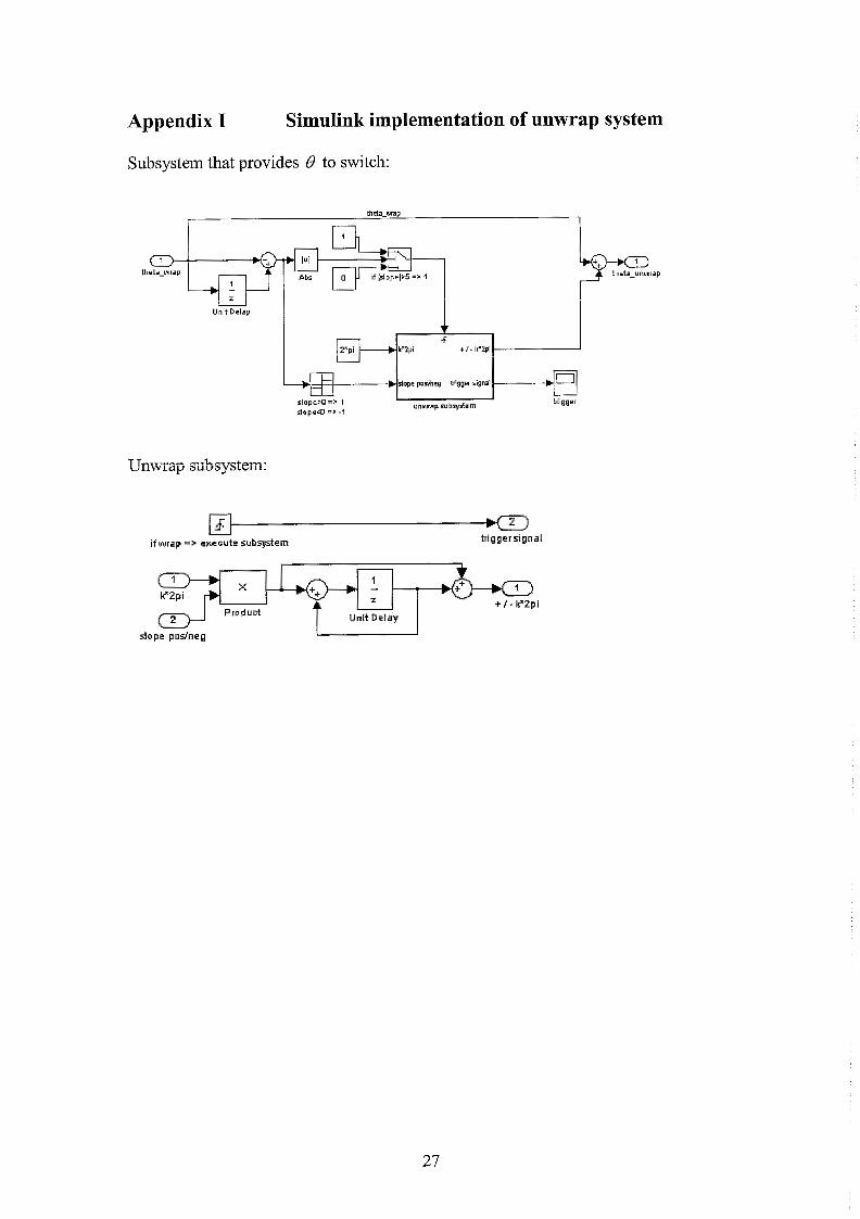
Appendix I Sirnulink implementation of unwrap system

Subsystem that provides 0 to switch:

theta-wnp

slope posheg tngger signal

unwrap s u b e m

if wrap => sxccute subqfstern

Appendix PI Simulink implementation of the filter

Implementation of the filter in Simulink

Matlab script for determination of feedback gain K.

q = 0.01; variance model r = l ; variance measurement uncertainties g = 0.5; weight factor for model uncertainties

sys = SS(A,[B G],C,[D HI); sysd = c2d(sys,dt); [a,b,c,d] = SSDATA(sysd); [KEST,L,P,M,Z] = KALMAN(sysd,Qn,Rn);

with L used as feedback gain K

Appendix I11 Q-basic script of tracking controller.

'CONTROL DRIVING A STRAIGHT LINE 'COMMANDS USED FROM EXAMPLE PROGRAM #l. 'QBASIC

'DRIVE STRAIGT LINE 'DIRECTION: 285 [DEG]

'OPEN THE SERIAL PORT. 'SET-W SCREEN. CLS

LOCATE 1, 1: PRINT " Compass: ";

LOOPCOUNT = 0

'COMPASS HEADING. PRINT #1, "!lGCl"; RO$ = INPUT$(4, #1) LOCATE 1,12 GOSUB WORDTODEC PRINTRO; "DEG "

'LOOPCOUNTER LOOPCOUNT = LOOPCOUNT + 1 PRTNT LOOPCOUNT;

'kleiner dan 281 :meer d m -4 graden afwijking IF RO < 281 THEN

'rotate +3 [DEG] OPDRACHT$ = " ! 1PN20" PRINT "DRAAI - RECHTS";

'groter d m 289:meer dan +4 graden afwij king ELSEIF RO > 289 THEN

'rotate -3 [DEG] OPDRACHT$ = " ! 1PN00" PRINT "DRAAI - LINKS";

landers vooruit ELSE

OPDRACHT$ = " ! 1 PN4 1 " PRINT "RLT - VOORUIT";

END IF

'voer commando uit PRINT #1, OPDRACHT$

'STOP IF KEY PRESSED. LOOP WHILE INKEY$ = ""

t n Lofive& - - a he-,~&&mz! word in RO$ to decimd ,!in RO WQRDTOOEC: R1$ = MID$(RO$, 1, 1) GOSTUB NBTBDEC RO = R1 * 4096 R1$ = MID$(RO$, 2, 1) GOSUB NIBTODEC RO = RO + (R1 * 256) R1$ = MID$(RO$, 3, 1) GOSUB NIBTODEC RO = RO + (R1 * 16) R1$ = MID$(RO$, 4, 1) GOSUB NIBTODEC RO=RO+Rl RETURN

'Convert a hexadecimal byte in RO$ to decimal in RO BYTETODEC: R1$ = MID$(RO$, 1, 1) GOSUB NIBTODEC RO=Rl * 16 R1$ = MID$(RO$, 2, 1) GOSUB NIBTODEC RO=RO+Rl RETURN

'Convert a hexadecimal nibble in R1$ to decimal in R1 NIBTODEC:

IF R1$ = "A" THEN R1= 10: RETURN IFRl$="B"THENRl=ll:RETURN IF R1$ = "C" THEN R1= 12: RETURN F R1$ = "Di' THEN Ri = 13: RET'uIRN II; R1$ = "E" THEN R1 = 14: RETURN IF R1$ = "F" THEN R1= 15: RETURN R1= VAL(Rl$)

RETURN

END

Appendix IV Matlab script of tracking controller.

function regelaarl clear all % MatLab version of tracking controller (already made in Q-basic)

% Define serial port s = serial('COM1'); % Connect fopen(s)

% Initialise Trilobot @rintf(s,'I 1THi 0 1:); f?ead(s, l ,'char'); % head straight @rintf(s,'! 1PEO1 I); fiead(s, 1 ,'charf); % set emergency stop

% Initialise parameters bt=O;i=O; koers=285; tic; tO=clock; heading=[] ; time =[I; stuurtot=[] ; time-act=[] ; time-cornpas=[] ; time-loop=[];

% start loop while bt=O: while bt==O

i=i+ 1 ; tloop0=clock;

% read compasslheading: tcom-pas0=clock; @rintf(s,'! 1 GC1 '); cr=hex2dec(char(fread(s,4,'char')')); % time needed for reading compass: time~compas=[time~compas etime(clock,tcompas0)]; % save heading in vector: heading=[heading cr];

if cr < koers-4 %&ai i -3 graden act=[ ('! 1PM02001008'}];disp('rechts') stuur=- 1 ;

elseif cr > koers+4 %draai -3 graden act=[{'! lPM02OOlOl 8'}];disp('links') stuur= 1 ;

else %rij vooruit

act=[('! 1PM02999900')];disp('voomit') stuur=o;

end

% save commands in vector: % (- 1 =left; 1 =right;O=straight) stuurtot=[stuurtot stuur];

% perfom actions: taciG=clsck; for k=l :length(act)

fprintf(s,act {k)); fread(s, 1 ,'charf); end %time needed for performing actions: time-act=[time-act etime(clock,tactO)];

% display results: disp(sprintf('%2i: compass: %3 .O f ,i,cr))

% stop loop if 35 loops are made: if i==3 5

bt=l ;disp('stopl) end % time needed for each loop: time~loop=[time~loop etime(clock,tloop0)]; % total time needed: time=[time etime(clock,tO)];

end

% stop commando: @rintf(s,'!PM00000100'); fread(s, 1 ,'char1);

% plotwork: figure(l);plot(time,heading) figure(2);plot(time7tirne~compas) figure(3);plot(time7time-act) figure(4);plot(time,time~loop,time,time~compas+time~act);legend('time- 1oop','time(compas+act)')

% save variables to workspace: control.mat save control

% Disconnect and clean up % -- When you no longer need s, you should disconnect it from the robot, % and remove it from memory and from the MATLAB workspace. fclose(s) delete(s) clear s

ret

Appendix V Sirnulink implementation of a trajectory generator

yd-r - d~ter rn ine v-r vref to uspace

reference m o w

4 w-rEf i

thetaref to wpace

Appendix VI Files

For the e-beam vou will need:

ML-worlung directory: -s-ebeam.dl1 (with s-ebeam.c and the MEX-compiler of Matlab the s-ebeam.dl1 can be compiled. S-ebeam.dl1 is an s-hct ion that is used in Matlab)

-WindowsKT-directory: -ebeam.dPP (unfortunately it was not possible to change this name, ebeamdll would be more appropriate. ebeam. cpp (C+ +), ebeam. dsw (project workspace), ebeantdsp (project files) and id%api.iz is needed to compile ebeam. dll) -Wbapi.dll (standard Ebeam manufacturer file)

Wintarget-directory: -&earn !cc.!ih (this kc.lih (library for lcc-compiler) is made with-a DOS- batch (make-ebeam lib.bat), which uses ebeam.dl1 to make the library, renames the ebeam.%b to ebeam-lcc.lib and copies it automatically to the wintarget directory) -In wt - 1cc.tmf there has to be a reference to ebeam-1cc.lib.

For the HMR vou will need: (Always execute the hypertenninal-test (hmrtest.ht) for the HMR3000 first, to open the connection) ML-working directory:

-sfun-hmrread.dl1 (with sfun-hmr7ead.c and the MEX-compiler of Matlab the sfun - hmrread.dl1 can be compiled. Sfun-hmrread.dl1 is an s-function, which is used in Matlab)

WindowsNT-directory: -hmrread.dll (hmrread.cpp, hmrread.dsw and hmrread.dsp are needed to compile hmrread. dll) -In wt - 1cc.tmf there has to be a reference to hmrread-1cc.lib.

Wintarget-directory: -hmrread-lcc.lib (made with: make-hmrreadlib. bat)

For the mouse you will need:

ML-working directory: -s-mouse.dll (with s- mouse.^ and the MEX-compiler of Matlab the s mouse.dl1 can be compiled. S-mouse.dl1 is an s-function, which is used in Mat lab)

WindowsNT-directory: -monse.dll mouse.^, mouse.dsw and mouse.dsp is needed to compile mouse.dll)

Wintarget-directory: - mouse-1cc.lib (made with: make-mouselib. bat)

- In wt - k t m f there has to be a reference to mouse-1cc.lib.

Bibliography

[ l ] Jakubiak J., Lefeber E., Tch6n K., Nijmeijer H. (2002): Two obsewer- based tracking algorithms for a unicycle mobile robot. - International Journal of Applied Mathematical Computational Science, Vol. 12, No. 4, pp 5 13-522.

[2] Noijen S.P.M. (2003): An orientation error observer for a unicycle mobile robot. - DCT 2003.65 - Eindhoven: TUE.

[S] Meij J'.J'.A.M. (2003): Obstacle avoidance for wheeled moSile robotic systems. - DCT 2003.11 - Eindhoven: TUE

[4] h c k Robotics (1998): Trilobot, mobile robot for research and education, user guide. - Hurst, Texas.

[5] Ricardo Sanz, Karl-Erik Arzkn (2003): Trends in Software and Control. - IEEE Control Systems Magazine, June 2003, vo1.23, No. 3,pp 12-1 5