control system theory and design
TRANSCRIPT

7/28/2019 Control System Theory and Design
http://slidepdf.com/reader/full/control-system-theory-and-design 1/290
Lecture Notes
Control Systems Theoryand Design
Herbert Werner

7/28/2019 Control System Theory and Design
http://slidepdf.com/reader/full/control-system-theory-and-design 2/290
Copyright c2009 Herbert Werner ([email protected])
Technische Universitat Hamburg-Harburg
ver. October 20, 2009

7/28/2019 Control System Theory and Design
http://slidepdf.com/reader/full/control-system-theory-and-design 3/290
Contents
Introduction vi
1 State Space Models 1
1.1 From Transfer Function to State Space Model . . . . . . . . . . . . . . . . 2
1.2 From State Space Model to Transfer Function . . . . . . . . . . . . . . . . 5
1.3 Changing Eigenvalues Via State Feedback . . . . . . . . . . . . . . . . . . 6
1.4 Non-Uniqueness of State Space Models and Similarity Transformations . . 8
1.5 Solutions of State Equations and Matrix Exponentials . . . . . . . . . . . . 10
2 Controllability and Pole Placement 20
2.1 The Controllability Gramian . . . . . . . . . . . . . . . . . . . . . . . . . . 21
2.2 The Controllability Matrix . . . . . . . . . . . . . . . . . . . . . . . . . . . 22
2.3 Pole Placement . . . . . . . . . . . . . . . . . . . . . . . . . . . . . . . . . 24
2.4 Uncontrollable Systems . . . . . . . . . . . . . . . . . . . . . . . . . . . . . 26
3 Observability and State Estimation 38
3.1 State Estimation . . . . . . . . . . . . . . . . . . . . . . . . . . . . . . . . 38
3.2 Unobservable Systems . . . . . . . . . . . . . . . . . . . . . . . . . . . . . 43
3.3 Kalman Canonical Decomposition . . . . . . . . . . . . . . . . . . . . . . . 46

7/28/2019 Control System Theory and Design
http://slidepdf.com/reader/full/control-system-theory-and-design 4/290
iv CONTENTS
4 Observer-Based Control 51
4.1 State Estimate Feedback . . . . . . . . . . . . . . . . . . . . . . . . . . . . 51
4.2 Reference Tracking . . . . . . . . . . . . . . . . . . . . . . . . . . . . . . . 53
4.3 Closed-Loop Transfer Function . . . . . . . . . . . . . . . . . . . . . . . . 57
4.4 Symmetric Root Locus Design . . . . . . . . . . . . . . . . . . . . . . . . . 59
5 Multivariable Systems 74
5.1 Transfer Function Models . . . . . . . . . . . . . . . . . . . . . . . . . . . 74
5.2 State Space Models . . . . . . . . . . . . . . . . . . . . . . . . . . . . . . . 76
5.3 The Gilbert Realization . . . . . . . . . . . . . . . . . . . . . . . . . . . . 78
5.4 Controllability and Observability . . . . . . . . . . . . . . . . . . . . . . . 79
5.5 The Smith-McMillan Form . . . . . . . . . . . . . . . . . . . . . . . . . . . 84
5.6 Multivariable Feedback Systems and Closed-Loop Stability . . . . . . . . . 86
5.7 A Multivariable Controller Form . . . . . . . . . . . . . . . . . . . . . . . . 89
5.8 Pole Placement . . . . . . . . . . . . . . . . . . . . . . . . . . . . . . . . . 92
5.9 Optimal Control of MIMO Systems . . . . . . . . . . . . . . . . . . . . . . 94
6 Digital Control 112
6.1 Discrete-Time Systems - z-Transform and State Space Models . . . . . . . 114
6.2 Sampled Data Systems . . . . . . . . . . . . . . . . . . . . . . . . . . . . . 124
6.3 Sampled-Data Controller Design . . . . . . . . . . . . . . . . . . . . . . . . 127
6.4 Frequency Response of Sampled-Data Systems . . . . . . . . . . . . . . . . 135
7 System Identification 147
7.1 Least Squares Estimation . . . . . . . . . . . . . . . . . . . . . . . . . . . 148
7.2 Estimation of Transfer Function Models . . . . . . . . . . . . . . . . . . . 151
7.3 Subspace Identification of State Space Models . . . . . . . . . . . . . . . . 155
7.4 Direct Subspace Identification . . . . . . . . . . . . . . . . . . . . . . . . . 160

7/28/2019 Control System Theory and Design
http://slidepdf.com/reader/full/control-system-theory-and-design 5/290
CONTENTS v
8 Model Order Reduction 167
9 Case Study: Modelling and Multivariable Control of a Process Evapo-rator 174
9.1 Evaporator Model . . . . . . . . . . . . . . . . . . . . . . . . . . . . . . . . 174
9.2 Control Objectives . . . . . . . . . . . . . . . . . . . . . . . . . . . . . . . 175
9.3 Modelling and Design . . . . . . . . . . . . . . . . . . . . . . . . . . . . . . 176
9.4 Controller Design Files . . . . . . . . . . . . . . . . . . . . . . . . . . . . . 176
9.5 Controller Design . . . . . . . . . . . . . . . . . . . . . . . . . . . . . . . . 177
A Vector Norms, Matrix Norms . . . 178
A.1 Vector Norms . . . . . . . . . . . . . . . . . . . . . . . . . . . . . . . . . . 178
A.2 The Matrix-2-Norm . . . . . . . . . . . . . . . . . . . . . . . . . . . . . . . 179
A.3 The Singular Value Decomposition . . . . . . . . . . . . . . . . . . . . . . 181
B Probability and Stochastic Processes 185
B.1 Probability and Random Variables . . . . . . . . . . . . . . . . . . . . . . 185
B.2 Stochastic Processes . . . . . . . . . . . . . . . . . . . . . . . . . . . . . . 195
B.3 Systems with Stochastic Inputs . . . . . . . . . . . . . . . . . . . . . . . . 205
C Solutions to Exercises 213
C.1 Chapter 1 . . . . . . . . . . . . . . . . . . . . . . . . . . . . . . . . . . . . 214
C.2 Chapter 2 . . . . . . . . . . . . . . . . . . . . . . . . . . . . . . . . . . . . 223
C.3 Chapter 3 . . . . . . . . . . . . . . . . . . . . . . . . . . . . . . . . . . . . 232
C.4 Chapter 4 . . . . . . . . . . . . . . . . . . . . . . . . . . . . . . . . . . . . 235
C.5 Chapter 5 . . . . . . . . . . . . . . . . . . . . . . . . . . . . . . . . . . . . 244
C.6 Chapter 6 . . . . . . . . . . . . . . . . . . . . . . . . . . . . . . . . . . . . 259
C.7 Chapter 7 . . . . . . . . . . . . . . . . . . . . . . . . . . . . . . . . . . . . 274
C.8 Chapter 8 . . . . . . . . . . . . . . . . . . . . . . . . . . . . . . . . . . . . 279
Bibliography 280

7/28/2019 Control System Theory and Design
http://slidepdf.com/reader/full/control-system-theory-and-design 6/290
Introduction
Classical techniques for analysis and design of control systems, which employ the concepts
of frequency response and root locus, have been used successfully for more than five
decades in a vast variety of industrial applications. These methods are based on transferfunction models of the plant to be controlled, and allow an efficient design of controllers
for single-input single-output systems. However, when it comes to more complex systems
with several input and output variables, classical techniques based on transfer functions
tend to become tedious and soon reach their limits. For such applications, the so-called
modern control techniques developed in the 1960s and 70s turned out to be more suitable.
They are based on state space models of the plant rather than on transfer function models.
One major advantage of state space models is that multi-input multi-output systems can
be treated in much the same way as single-input single-output systems. This course
provides an introduction to the modern state space approach to control and its theoretical
foundations.
State space models are introduced in Chapter 1; to facilitate the understanding of the
basic concepts, the discussion is initially limited to single-input single-output systems.
The main idea - introduced in Chapters 1 through 4 - is to break the controller design
problem up in two subproblems: (i) the problem of designing a static controller that
feeds back internal variables - the state variables of the plant, and (ii) the problem of
obtaining a good estimate of these internal state variables. It is shown that these two
problems are closely related, they are called dual problems . Associated with state feedback
control and state estimation (the latter is usually referred to as state observation ) are the
concepts of controllability and observability. In Chapter 5 these concepts are extended
to multivariable systems, and it will be seen that this extension is in most aspects rather
straightforward, even though the details are more complex.
A further important topic, discussed in Chapter 6, is the digital implementation of con-
trollers. It is shown that most of the methods and concepts developed for continuous-time
systems have their direct counterparts in a discrete-time framework. This is true for trans-
fer function models as well as for state space models.
The third major issue taken up in this course is about obtaining a model of the plant to be
controlled. In practice, a model is often obtained from experimental data; this approachis known as system identification . In Chapter 7 the basic ideas of system identification

7/28/2019 Control System Theory and Design
http://slidepdf.com/reader/full/control-system-theory-and-design 7/290
Introduction vii
are introduced; identification of transfer function models as well as state space models are
discussed. In Chapter 8 the issue of reducing the dynamic order of a model is addressed -
this can be important in applications where complex plant models lead to a large number
of state variables.
Most chapters are followed by a number of exercise problems. The exercises play an
important role in this course. To encourage student participation and active learning,
derivations of theoretical results are sometimes left as exercises. A second objective is to
familiarize students with the state-of-the-art software tools for modern controller design.
For this reason, a number of analysis and design problems are provided that are to be
solved using MATLAB and Simulink. MATLAB code and Simulink models for these
problems can be downloaded from the web page of this course. A complete design exercise
that takes up all topics of this course - identification of a model, controller and observerdesign and digital implementation - is presented in Chapter 9.
This course assumes familiarity with elementary linear algebra, and with engineering
applications of some basic concepts of probability theory and stochastic processes, such
as white noise. A brief tutorial introduction to each of these fields is provided in the
Appendix. The Appendix also provides worked solutions to all exercises. Students are
encouraged to try to actively solve the exercise problems, before checking the solutions.
Some exercises that are more demanding and point to more advanced concepts are marked
with an asterisk.
The exercise problems and worked solutions for this course were prepared by MartynDurrant MEng.

7/28/2019 Control System Theory and Design
http://slidepdf.com/reader/full/control-system-theory-and-design 8/290

7/28/2019 Control System Theory and Design
http://slidepdf.com/reader/full/control-system-theory-and-design 9/290
Chapter 1
State Space Models
In this chapter we will discuss linear state space models for single-input single-output
systems. The relationship between state space models and transfer function models is
explored, and basic concepts are introduced.
u
y
k b
m
Figure 1.1: Spring-mass-damper system
We begin with an example. Consider the spring-mass-damper system shown in Fig.1.1
with mass m, spring constant k and damping coefficient b. The equation of motion is
y(t) +b
my(t) +
k
my(t) =
1
mu(t). (1.1)
where u(t) is an external force acting on the mass and y(t) is the displacement from
equilibrium. From the equation of motion, the transfer function is easily found to be
G(s) =1
m
s2 + bm
s + km
(1.2)
Introducing the velocity v = y as a new variable, it is straightforward to check that the
second order differential equation (1.1) can be rewritten as a first order vector differential
equation y(t)
v(t)
= 0 1
−k/m −b/m
y(t)
v(t)
+ 0
1/m
u(t) (1.3)

7/28/2019 Control System Theory and Design
http://slidepdf.com/reader/full/control-system-theory-and-design 10/290
2 1. State Space Models
together with an output equation
y(t) = [1 0] y(t)
v(t) (1.4)
The model (1.3), (1.4) describes the same dynamic properties as the transfer function
(1.2). It is a special case of a state space model
x(t) = Ax(t) + Bu(t) (1.5)
y(t) = Cx(t) + Du(t) (1.6)
In general, a system modelled in this form can have m inputs and l outputs, which are
then collected into an input vector u(t) ∈ IRm and an output vector y(t) ∈ IRl. The vector
x(t)
∈IRn is called state vector , A
∈IRn×n is the system matrix , B
∈IRn×m is the input
matrix , C ∈ IRl×n is the output matrix and D ∈ IRl×m is the feedthrough matrix . Equation
(1.5) is referred to as the state equation and (1.6) as the output equation .
The spring-mass-damper system considered above has only one input and one output.
Such systems are called single-input single-output (SISO) systems, as opposed to multi-
input multi-output (MIMO) systems. For a SISO system the input matrix B degenerates
into a column vector b, the output matrix C into a row vector c and the feedthrough
matrix D into a scalar d. Initially, we will limit the discussion of state space models to
SISO systems of the form
x(t) = Ax(t) + bu(t) (1.7)y(t) = cx(t) + du(t) (1.8)
In the above example the direct feedthrough term d is zero - this is generally true for
physically realizable systems, as will be discussed later.
1.1 From Transfer Function to State Space Model
The state space model (1.3), (1.4) for the second order system in the above example was
constructed by introducing a single new variable. We will now show a general method for
constructing a state space model from a given transfer function. Consider the nth order
linear system governed by the differential equation
dn
dtny(t) + an−1
dn−1
dtn−1y(t) + . . . + a1d
dty(t) + a0y(t) =
bmdm
dtmu(t) + bm−1
dm−1
dtm−1u(t) + . . . + b1d
dtu(t) + b0u(t) (1.9)
where we assume for simplicity that the system is strictly proper, i.e. n > m (the case of
bi-proper systems is discussed at the end of this section). A transfer function model of
this system is
Y (s) = G(s)U (s) (1.10)

7/28/2019 Control System Theory and Design
http://slidepdf.com/reader/full/control-system-theory-and-design 11/290
1.1. From Transfer Function to State Space Model 3
where
G(s) =bmsm + bm−1sm−1 + . . . + b1s + b0
sn + an
−1sn−1 + . . . + a1s + a0
=b(s)
a(s)(1.11)
u(t) y(t)b(s)a(s)
Figure 1.2: Transfer function model
The transfer function model of this system is shown in Fig. 1.2. In order to find a state
space model for this system, we will first construct a simulation model by using integrator
blocks. For this purpose, we split the model in Fig. 1.2 into two blocks as shown in Fig.
1.3, and let v(t) denote the fictitious output of the filter 1/a(s).
1a(s)
u(t) b(s) y(t)v(t)
Figure 1.3: Transfer function model
From Fig. 1.3 the input and output signals can be expressed in terms of the new variable
as U (s) = a(s)V (s) and Y (s) = b(s)V (s), or in time domain
u(t) = dn
dtnv(t) + an−1 d
n−1
dtn−1v(t) + . . . + a1 ddt
v(t) + a0v(t) (1.12)
and
y(t) = bmdm
dtmv(t) + bm−1
dm−1
dtm−1v(t) + . . . + b1d
dtv(t) + b0v(t) (1.13)
From (1.12) the signal v(t) can be generated by using a chain of integrators: assume first
that dnv(t)/dtn is somehow known, then integrating n times, introducing feedback loops
as shown in the lower half of Fig. 1.4 (for n = 3 and m = 2) and adding the input signal
u(t) yields the required signal dnv(t)/dtn. The output signal y(t) can then be constructed
as a linear combination of v(t) and its derivatives according to (1.13), as shown in the
upper half of Fig. 1.4.
An implicit assumption was made in the above construction: namely that the initial values
at t = 0 in (1.12) and (1.13) are zero. In the model in Fig. 1.4 this corresponds to the
assumption that the integrator outputs are zero initially. When transfer function models
are used, this assumption is usually made, whereas state space models allow non-zero
initial conditions to be taken into account.
State Variables
Before we derive a state space model from the simulation model in Fig. 1.4, we introduce
the concept of state variables . For a given system, a collection of internal variables
x1(t), x2(t), . . . , xn(t)

7/28/2019 Control System Theory and Design
http://slidepdf.com/reader/full/control-system-theory-and-design 12/290
4 1. State Space Models
v
−a1
−a0
−a2
x1
u y
b2
b1
b0v vv
x3
...
x3 = x2 x2 = x1
Figure 1.4: Simulation model for system (1.9) when n = 3 and m = 2
is referred to as state variables if they completely determine the state of the system at
time t. By this we mean that if the values of the state variables at some time, say t0,
are known, then for a given input signal u(t) where t ≥ t0 all future values of the state
variables can be uniquely determined. Obviously, for a given system the choice of state
variables is not unique.
We now return to the system represented by the simulation model in Fig. 1.4. Here the
dynamic elements are the integrators, and the state of the system is uniquely determined
by the values of the integrator outputs at a given time. Therefore, we choose the integrator
outputs as state variables of the system, i.e. we define
x1(t) = v(t), x2(t) =d
dtv(t), . . . , xn(t) =
dn−1
dtn−1v(t)
The chain of integrators and the feedback loops determine the relationship between the
state variables and their derivatives. The system dynamics can now be described by a set
of first order differential equations
x1 = x2
x2 = x3
...
xn−1 = xn
xn = u − a0x1 − a1x2 − . . . − an−1xn
The last equation is obtained at the input summing junction in Fig. 1.4. The first order
differential equations can be rewritten in vector form: introduce the state vector
x(t) = [x1(t) x2(t) . . . xn(t)]T

7/28/2019 Control System Theory and Design
http://slidepdf.com/reader/full/control-system-theory-and-design 13/290
1.2. From State Space Model to Transfer Function 5
then we have
x1
x2...
xn−1xn
=
0 1 0 . . . 0
0 0 1 0.... . .
...
0 0 0 . . . 1
−a0 −a1 −a2 . . . −an−1
x1
x2...
xn−1xn
+
0
0...
0
1
u(t) (1.14)
This equation has the form of (1.7) and is a state equation of the system (1.9). The
state equation describes the dynamic properties of the system. If the system is physically
realizable, i.e. if n > m, then from (1.13) and Fig. 1.4, the output signal is a linear
combination of the state variables and can be expressed in terms of the state vector as
y(t) = [b0 b1 . . . bn−1]
x1x2...
xn
(1.15)
This equation has the form of (1.8) and is the output equation of the system (1.9) associ-
ated with the state equation (1.14). The system matrices (vectors) A, b and c of this state
space model contain the same information about the dynamic properties of the system as
the transfer function model (1.11). As mentioned above, the choice of state variables for
a given system is not unique, and other choices lead to different state space models for
the same system (1.9). For reasons that will be discussed later, the particular form (1.14)and (1.15) of a state space model is called controller canonical form . A second canonical
form, referred to as observer canonical form , is considered in Exercise 1.8.
Note that for bi-proper systems, i.e. systems where n = m, there will be a feedthrough
term du(t) in (1.15); if the example in Figure 1.4 was bi-proper there would be a direct
path with gain b3 from d3v/dt3 to y.
1.2 From State Space Model to Transfer Function
We have seen how a particular state space model of a system can be constructed when its
transfer function is given. We now consider the case where a state space model is given
and we wish to find its transfer function. Thus, consider a system described by the state
space model
x(t) = Ax(t) + bu(t)
y(t) = cx(t) + du(t)
and assume again that the initial conditions are zero, i.e. x(0) = 0. Taking Laplace
transforms, we have
sX (s) = AX (s) + bU (s)

7/28/2019 Control System Theory and Design
http://slidepdf.com/reader/full/control-system-theory-and-design 14/290
6 1. State Space Models
and solving for X (s) yields
X (s) = (sI − A)−1bU (s) (1.16)
where I denotes the identity matrix. Substituting the above in the Laplace transform of the output equation leads to
Y (s) = c(sI − A)−1bU (s) + dU (s)
Comparing this with the transfer function model (1.10) yields
G(s) = c(sI − A)−1b + d (1.17)
Further insight into the relationship between transfer function and state space model can
be gained by noting that
(sI − A)−1 =1
det(sI − A)adj (sI − A)
where adj (M ) denotes the adjugate of a matrix M . The determinant of sI − A is a
polynomial of degree n in s. On the other hand, the adjugate of sI − A is an n × n
matrix whose entries are polynomials in s of degree less than n. Substituting in (1.17)
and assuming n > m (i.e. d = 0) gives
G(s) =c adj(sI − A)b
det(sI −
A)
The adjugate is multiplied by the row vector c from the left and by the column vector b
from the right, resulting in a single polynomial of degree less than n. This polynomial is
the numerator polynomial of the transfer function, whereas det(sI −A) is the denominator
polynomial. The characteristic equation of the system is therefore
det(sI − A) = 0
Note that the characteristic equation is the same when there is a direct feedthrough term
d
= 0. The values of s that satisfy this equation are the eigenvalues of the system matrix
A. This leads to the important observation that the poles of the transfer function - which
determine the dynamic properties of the system - can be found in a state space model as
eigenvalues of the system matrix A.
1.3 Changing Eigenvalues Via State Feedback
A block diagram representing the state space model (1.7), (1.8) is shown in Fig. 1.5.
Note that no graphical distinction is made between scalar signals and vector signals. The
integrator block represents n integrators in parallel. When the relationship between state
space models and transfer functions was discussed, we assumed x(0) = 0. From now on

7/28/2019 Control System Theory and Design
http://slidepdf.com/reader/full/control-system-theory-and-design 15/290
1.3. Changing Eigenvalues Via State Feedback 7
ux
A
b
x(0)
xc y
Figure 1.5: Block diagram of SISO state space model
we will include the possibility of non-zero initial values of the state variables in the state
space model. In Fig. 1.5 this is done by adding the initial values to the integrator outputs.
The dynamic properties of this system are determined by the eigenvalues of the system
matrix A. Suppose we wish to improve the dynamic behaviour - e.g. when the system is
unstable or has poorly damped eigenvalues. If all state variables are measured, we can
use them for feedback by taking the input as
u(t) = f x(t) + uv(t) (1.18)
where f = [f 1 f 2 . . . f n] is a gain vector, and uv(t) is a new external input. This type of
feedback is called state feedback , the resulting closed-loop system is shown in Fig. 1.6.
f
uuv
x
A
b
x(0)
xc y
Figure 1.6: State feedback
Substituting (1.18) in the state equation yields
x(t) = Ax(t) + b(f x(t) + uv(t))
= (A + bf )x(t) + buv(t)
Comparing this with the original state equation shows that as a result of state feedback
the system matrix A is replaced by A + bf , and the control input u(t) is replaced by uv(t).

7/28/2019 Control System Theory and Design
http://slidepdf.com/reader/full/control-system-theory-and-design 16/290
8 1. State Space Models
The eigenvalues of the closed-loop system are the eigenvalues of A + bf , and the freedom
in choosing the state feedback gain vector f can be used to move the eigenvalues of the
original system to desired locations; this will be discussed later (see also Exercise 1.7).
1.4 Non-Uniqueness of State Space Models and
Similarity Transformations
The state variables we chose for the spring-mass-damper system have a physical meaning
(they represent position and velocity). This is often the case when a state space model is
derived from a physical description of the plant. In general however state variables need
not have any physical significance. The signals that represent the interaction of a systemwith its environment are the input signal u(t) and the output signal y(t). The elements
of the state vector x(t) on the other hand are internal variables which are chosen in a way
that is convenient for modelling internal dynamics; they may or may not exist as physical
quantities. The solution x(t) of the forced vector differential equation x(t) = Ax(t)+bu(t)
with initial condition x(0) = x0 can be thought of as a trajectory in an n-dimensional
state space , which starts at point x0. The non-uniqueness of the choice of state variables
reflects the freedom of choosing a coordinate basis for the state space. Given a state space
model of a system, one can generate a different state space model of the same system by
applying a coordinate transformation.To illustrate this point, consider a system modelled as
x(t) = Ax(t) + bu(t), x(0) = x0
y(t) = cx(t) + du(t)
A different state space model describing the same system can be generated as follows. Let
T be any non-singular n × n matrix, and consider a new state vector x(t) defined by
x(t) = T x(t)
Substituting in the above state space model gives
T ˙x(t) = AT x(t) + bu(t)
or˙x(t) = T −1AT x(t) + T −1bu(t)
and
y(t) = cT x(t) + du(t)
Comparing this with the original model shows that the model (A,b,c,d) has been replaced
by a model (˜
A,˜b, c, d), where
A = T −1AT, b = T −1b, c = cT

7/28/2019 Control System Theory and Design
http://slidepdf.com/reader/full/control-system-theory-and-design 17/290
1.4. Non-Uniqueness of State Space Models and Similarity Transformations 9
Note that the feedthrough term d is not affected by the transformation, because it is not
related to the state variables.
In matrix theory, matrices A and A related by
A = T −1AT
where T is nonsingular, are said to be similar , and the above state variable transformation
is referred to as a similarity transformation . Similarity transformations do not change the
eigenvalues, we have
det(sI − A) = det(sI − T −1AT ) = det(T −1(sI − A)T ) = det(sI − A)
In fact, it is straightforward to check that the models (A,b,c) and (˜
A,˜b, c) have the same
transfer function (see Exercise 1.9).
To see that T represents a change of coordinate basis, write x = T x as
x = [t1 t2 . . . tn]
x1
x2...
xn
= t1x1 + t2x2 + . . . + tnxn
where ti is the i
th
column of T . Thus, xi is the coordinate of x in the direction of thebasis vector ti. In the original coordinate basis, the vector x is expressed as
x = e1x1 + e2x2 + . . . + enxn
where ei is a vector with zeros everywhere except for the ith element which is 1.
We have thus seen that for a given transfer function model, by choosing a nonsingular
transformation matrix T we can find infinitely many different but equivalent state space
models. As a consequence, it is not meaningful to refer to the state variables of a system ,
but only of the state variables of a particular state space model of that system. Conversely,
all state space models that are related by a similarity transformation represent the samesystem. For this reason, a state space model is also referred to as a particular state space
realization of a transfer function model.
Diagonal Form
To illustrate the idea of a similarity transformation, assume that we are given a 3rd order
state space model (A,b,c) and that the eigenvalues of A are distinct and real. Suppose we
wish to bring this state space model into a form where the new system matrix is diagonal.
We need a transformation such that
A = T −1AT = Λ

7/28/2019 Control System Theory and Design
http://slidepdf.com/reader/full/control-system-theory-and-design 18/290
10 1. State Space Models
where Λ = diag (λ1, λ2, λ3). It is clear that the λi are the eigenvalues of A. To find the
required transformation matrix T , note that AT = T A or
A[t1 t2 t3] = [t1 t2 t3]
λ1 0 00 λ2 0
0 0 λ3
Looking at this equation column by column, we find that
Ati = λiti, i = 1, 2, 3
Therefore, the columns of T are the (right) eigenvectors of A. Since we assumed that
the eigenvalues of A are distinct, the three eigenvectors are linearly independent and T is
non-singular as required.
State space models with a diagonal system matrix are referred to as modal canonical
form , because the poles of a system transfer function (the eigenvalues appearing along
the diagonal) are sometimes called the normal modes or simply the modes of the system.
1.5 Solutions of State Equations and Matrix
Exponentials
We now turn to the solution of the forced vector differential equation
x(t) = Ax(t) + bu(t), x(0) = x0
First, we consider the scalar version of this problem
x(t) = ax(t) + bu(t), x(0) = x0
where x(t) is a single state variable and a is a real number. The solution to this problem
can be found by separating variables: we have
d
dt
e−atx
= e−at(x − ax) = e−atbu
Integration from 0 to t and multiplication by eat yields
x(t) = eatx0 +
t
0
ea(t−τ )bu(τ )dτ
Crucial for finding the solution in this scalar case is the property
d
dteat = aeat

7/28/2019 Control System Theory and Design
http://slidepdf.com/reader/full/control-system-theory-and-design 19/290
1.5. Solutions of State Equations and Matrix Exponentials 11
of the exponential function. To solve the state equation when x ∈ IRn, we would need
something liked
dt eAt
= AeAt
for a n × n matrix A. This leads to the definition of the matrix exponential
eAt = I + At +1
2!A2t2 +
1
3!A3t3 + . . . (1.19)
It can be shown that this power series converges. Differentiating shows that
d
dteAt = A + A2t +
1
2!A3t2 +
1
3!A4t3 + . . .
= A(I + At +1
2!A2t2 +
1
3!A3t3 + . . .)
= AeAt
as required. Incidentally, this also shows that AeAt = eAtA because A can be taken as a
right factor in the second equation above.
The solution of the state equation can thus be written as
x(t) = eAtx0 +
t
0
eA(t−τ )bu(τ )dτ
The transition matrix Φ(t) of a state space model is defined as
Φ(t) = eAt
With this definition, the solution becomes
x(t) = Φ(t)x0 +
t
0
Φ(t − τ )bu(τ )dτ (1.20)
The first term on the right hand side is called the zero-input response , it represents the
part of the system response that is due to the initial state x0. The second term is called
the zero-initial-state response , it is the part of the response that is due to the external
input u(t).
The frequency domain expression (1.16) of the solution was derived by assuming a zero
initial state. When the initial state is non-zero, it is easy to verify that the Laplace
transform of x(t) is
X (s) = Φ(s)x0 + Φ(s)bU (s) (1.21)
where
Φ(s) = L[Φ(t)σ(t)] = (sI − A)−1
is the Laplace transform of the transition matrix. The second equation follows directly
from comparing the expression obtained for X (s) with the time-domain solution (1.20).

7/28/2019 Control System Theory and Design
http://slidepdf.com/reader/full/control-system-theory-and-design 20/290
12 1. State Space Models
The definition of Φ(t) implies that this matrix function is invertible, we have
Φ−1(t) = e−At = Φ(
−t)
Another useful property of Φ(t) was shown above, namely:
AΦ(t) = Φ(t)A
Stability
From the study of transfer function models we know that a system is stable if all its
poles are in the left half plane. For a transfer function model, stability means that after
a system has been excited by an external input, the transient response will die out and
the output will settle to a new equilibrium value once the external stimulus has beenremoved. Since we have seen that poles of a transfer function become eigenvalues of the
system matrix A of a state space model, we might ask whether stability of a state space
model is equivalent to all eigenvalues of A being in the left half plane. In contrast to
transfer function models, the output of a state space model is determined not only by
the input but also by the initial value of the state vector. The notion of stability used
for transfer functions is meaningful for the part of the system dynamics represented by
the zero-initial-state response, but we also need to define stability with respect to the
zero-input response, i.e. when an initial state vector x(0) = 0 is driving the system state.
Definition 1.1 An unforced system x(t) = Ax(t) is said to be stable if for all x(0) = x0, x0 ∈ IR we have x(t) → 0 as t → ∞.
Now consider the zero-input response
x(t) = eAtx0
or in frequency domain
X (s) = (sI − A)−1x0
Assuming that the eigenvalues are distinct, a partial fraction expansion reveals that
x(t) = φ1eλ1t + . . . + φneλnt
where λi are the eigenvalues of A, and φi are column vectors that depend on the residual
at λi. It is clear that x(t) → 0 if only if all eigenvalues have negative real parts. Thus, we
find that stability with respect to both zero-initial state response and zero-input response
requires that all eigenvalues of A are in the left half plane.
The Cayley-Hamilton Theorem
We conclude this chapter with an important result on the representation of the transition
matrix. The following is derived (for the case of distinct eigenvalues) in Exercise 1.3:

7/28/2019 Control System Theory and Design
http://slidepdf.com/reader/full/control-system-theory-and-design 21/290
1.5. Solutions of State Equations and Matrix Exponentials 13
Theorem 1.1 (Cayley-Hamilton Theorem)
Consider a matrix A∈
IRn×n. Let
det(sI − A) = a(s) = sn + an−1sn−1 + . . . + a1s + a0 = 0
be its characteristic equation. Then
An + an−1An−1 + . . . + a1A + a0I = 0
In the last equation the 0 on the right hand side stands for the n × n zero matrix. This
theorem states that every square matrix satisfies its characteristic equation.
With the help of the Cayley-Hamilton Theorem we can express the matrix exponential
eAt - defined as an infinite power series - as a polynomial of degree n
−1. Recall the
definition
eAt = I + At +1
2!A2t2 +
1
3!A3t3 + . . . +
1
n!Antn + . . . (1.22)
From Theorem 1.1 we have
An = −an−1An−1 − . . . − a1A − a0I
and we can substitute the right hand side for An in (1.22). By repeating this, we can in fact
reduce all terms with powers of A greater than n to n − 1. Alternatively, we can achieve
the same result by polynomial division. Let a(s) = det(sI − A) be the characteristic
polynomial of A with degree n, and let p(s) be any polynomial of degree k > n. We can
divide p(s) by a(s) and obtain p(s)
a(s)= q (s) +
r(s)
a(s)
where the remainder r(s) has degree less than n. Thus, p(s) can be written as
p(s) = a(s)q (s) + r(s)
Replacing s as variable by the matrix A, we obtain the matrix polynomial equation
p(A) = a(A)q (A) + r(A) = r(A)
where the second equation follows from a(A) = 0. Since the polynomial p was arbitrary,
this shows that we can reduce any matrix polynomial in A to a degree less than n. Thisis also true for the infinite polynomial in (1.22), and we have the following result.
Theorem 1.2
The transition matrix of an nth-order state space model can be written in the form
Φ(t) = α0(t)I + α1(t)A + α2(t)A2 + . . . + αn−1(t)An−1 (1.23)
Note that the polynomial coefficients are time-varying, because the coefficients of the
infinite polynomial (1.22) are time-dependent. One way of computing the functions αi(t)for a given state space model is suggested in Exercise 1.5.

7/28/2019 Control System Theory and Design
http://slidepdf.com/reader/full/control-system-theory-and-design 22/290
14 1. State Space Models
Exercises
Problem 1.1
This exercise is a short revision of the concept of linearisation of physical model equations.
Consider the water tank in Figure 1.7.
0
f in
f out
= uValve positionh
Figure 1.7: State feedback
With the notation
At tank cross sectional area
h water height
f in inlet flow rate (vol/sec)
f out outlet flow rate (vol/sec)
P hydrostatic pressure at the tank’s bottom
u valve position
the relationships between pressure and water depth, and pressure and water flow out of
the tank are given by
P = hρg
f out = kv
√ P u
a) Describe the relationship between water height h, inflow f in and valve position u by
a differential equation. Why is this not linear?
b) Determine the valve position u0, that for a constant water height h0 and inflow f in0
keeps the level in the tank constant.
c) Show that for small deviations δh, δu of h and u, respectively, from a steady state
(h0,u0) the following linear approximation can be used to describe the water level

7/28/2019 Control System Theory and Design
http://slidepdf.com/reader/full/control-system-theory-and-design 23/290
Exercises 15
dynamics, where kt =√
ρgkv:
δ h =−
f in0
2Ath0δh
−kt
At h0δu
Hint: Use the Taylor-series expansion of f (h + δ ) for small δ
d) Write down the transfer function of the system at the linearised operating point
around the steady state (h0,u0). Identify the steady state process gain and the time
constant of the linearised system.
e) For the linearised system in (c) with input u and output h, determine a state space
model of the form
x = Ax + buy = Cx + du
Problem 1.2
Consider the circuit in Figure 1.8.
+ −
L
vl
C R
i
vs
vcvr
Figure 1.8: State feedback
a) Show that the voltage vr over the resistance R can be described by the state space
representation
x = Ax + bu, y = cx
where
x =
i
vc
, u = vs, y = vr
A = −R/L −1/L
1/C 0 , b = 1/L
0 , c = R 0Use the physical relationships vs = vc + vl + vr, vl = L di
dt, i = C dvc
dt.

7/28/2019 Control System Theory and Design
http://slidepdf.com/reader/full/control-system-theory-and-design 24/290
16 1. State Space Models
b) Show that the circuit can also be described by the following differential equation:
LC d2vc
dt2+ RC
dvc
dt+ vc = vs
c) Write this equation in state space form with state variables x1 = vc and x2 = vc.
Problem 1.3
Consider a matrix A ∈ IRn×n with the characteristic polynomial
det (sI − A) = a(s) = sn + an−1sn−1 + . . . + a1s + a0
a) Show that if A has distinct eigenvalues (λ1, λ2 . . . λn), the following relationshipholds:
Λn + an−1Λn−1 + . . . + a0I = 0
with Λ =
λ1 0 . . . 0
0 λ2 . . . 0...
.... . .
...
0 . . . 0 λn
Hint: use the fact that a matrix A with distinct eigenvalues can be written as A =
T −1ΛT ; where Λ is diagonal.
b) Now show that
An + an−1An−1 + . . . + a0I = 0
(This proves the Cayley-Hamilton Theorem for distinct eigenvalues)
Problem 1.4
Consider the homogeneous 2 × 2 system
x = Ax
where the distinct, real eigenvalues of A are λ1 and λ2 with corresponding eigenvectors t1and t2.
a) Using the Laplace transform
sX (s) − x(0) = AX (s)
show that
X (s) = T 1
s−λ10
0 1s−λ2T −1x(0), T = [t1 t2]
where ti are the columns of T .

7/28/2019 Control System Theory and Design
http://slidepdf.com/reader/full/control-system-theory-and-design 25/290
Exercises 17
b) Show that with the initial condition
x(0) = kt1
we have
X (s) =1
s − λ1
t1
c) For
A =
−1 1
−2 −4
Plot, using MATLAB, the behaviour of the system in a phase plane diagram (i.e.
sketch x2(t) over x1(t) as t goes from zero to infinity) for the initial values of the
state vector
i) x(0) = t1
ii) x(0) = t2
Problem 1.5
a) Use the fact that the eigenvalues of A are solutions of the characteristic equation to
show that eλit for all eigenvalues λ = λ1, λ2 . . . λn can be expressed as
eλt = α0(t) + α1(t)λ + . . . + αn−1(t)λn−1
b) By considering this identity for each of the eigenvalues, determine the functions
αi(t), i = 1, . . . , n − 1 in (1.23). Assume that the eigenvalues are distinct.
Hint: Use the fact that for distinct eigenvalues the following matrix is invertible:
1 λ1 . . . λn−11
1 λ2 . . . λn−12
.
..... . . .
.
..1 λn . . . λn−1
n
Problem 1.6
Consider the system x = Ax + bu with
A =
−6 2
−6 1
, b =
1
0, c =
1 1a) Use the results from Problem 1.5 to calculate the functions α0(t), α1(t) and eAt.

7/28/2019 Control System Theory and Design
http://slidepdf.com/reader/full/control-system-theory-and-design 26/290
18 1. State Space Models
b) Calculate the state and output responses, x(t) and y(t), with initial values x(0) =
2 1
T
c) Calculate the output response with initial values from (b) and a step input u(t) =
2σ(t)
Problem 1.7
a) Convert the 2nd order model of the spring mass system (1.1) into the controllercanonical form. Use the values
m = 1, k = 1, b = 0.1
b) For this model, calculate (sI − A)−1 and c(sI − A)−1b.
c) Calculate gain matrix f = [f 1 f 2] for a state feedback controller u = f x, which will
bring the system with an initial state of x(0) = [1 0]T back to a steady state with asettling time (1%) ts ≤ 5 and with damping ratio ζ ≥ 0.7.
d) Calculate f , using MATLAB, for the settling time ts ≤ 5 and damping ratio ζ ≥ 0.7.
Hint: Consider the characteristic polynomial of the closed loop system.
Problem 1.8
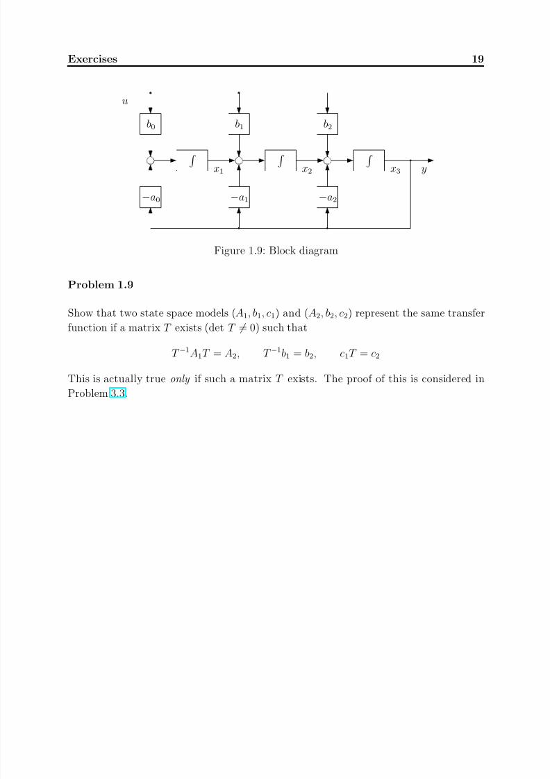
Consider the system in Figure 1.9.
Determine a state space model with states x1, x2, x3 for this system. Show that the
transfer function of this system is
Y (s) =b2s2 + b1s + b0
s3 + a2s2 + a1s1 + a0U (s)
(This particular state space representation is called the observer canonical form .)
7/28/2019 Control System Theory and Design
http://slidepdf.com/reader/full/control-system-theory-and-design 27/290
Exercises 19
y
b0
x1
−a1−a0
b1 b2
x2 x3
−a2
u
Figure 1.9: Block diagram
Problem 1.9
Show that two state space models (A1, b1, c1) and (A2, b2, c2) represent the same transfer
function if a matrix T exists (det T = 0) such that
T −1A1T = A2, T −1b1 = b2, c1T = c2
This is actually true only if such a matrix T exists. The proof of this is considered in
Problem 3.3.

7/28/2019 Control System Theory and Design
http://slidepdf.com/reader/full/control-system-theory-and-design 28/290
Chapter 2
Controllability and Pole Placement
This chapter will introduce the first of two important properties of linear systems that
determine whether or not given control objectives can be achieved. A system is said to be
controllable if it is possible to find a control input that takes the system from any initial
state to any final state in any given time interval. In this chapter, necessary and sufficient
conditions for controllability are derived. It is also shown that the closed-loop poles can
be placed at arbitrary locations by state feedback if and only if the system is controllable.
We start with a definition of controllability. Consider a system with state space realization
x(t) = Ax(t) + bu(t) (2.1)
y(t) = cx(t)
Definition 2.1
The system (2.1) is said to be controllable if for any initial state x(0) = x0, time tf > 0
and final state xf there exists a control input u(t), 0 ≤ t ≤ tf , such that the solution of
(2.1) satisfies x(tf ) = xf . Otherwise, the system is said to be uncontrollable.
Since this definition involves only the state equation, controllability is a property of thedata pair (A, b).
Example 2.1
As an example of an uncontrollable system, considerx1(t)
x2(t)
=
λ 0
0 λ
x1(t)
x2(t)
+
1
1
u(t), x0 =
0
0
, xf =
2
3
From the solution of the state equation
x1(t) = x2(t) =
t
0
eλ(t−τ )u(τ )dτ

7/28/2019 Control System Theory and Design
http://slidepdf.com/reader/full/control-system-theory-and-design 29/290
2.1. The Controllability Gramian 21
and it is clear that there exists no input u(t) that will bring the system to the final state
xf .
2.1 The Controllability Gramian
Returning to the system (2.1), controllability requires that there exists an input u(t) on
the interval 0 ≤ t ≤ tf such that
xf = eAtf x0 +
tf
0
eA(tf −τ )bu(τ )dτ (2.2)
To establish conditions for the existence of such a control input, we will first present a
particular choice of input that satisfies (2.2) under the assumption that a certain matrix
is invertible. We will then show that if (2.1) is controllable, this assumption is always
true.
Thus, consider the input
u(t) = −bT eAT (tf −t)W −1c (tf )(eAtf x0 − xf ) (2.3)
where the matrix W c(t) ∈ IRn×n is defined as
W c(t) = t
0 eAτ
bbT
eAT τ
dτ (2.4)
That this input takes the system from x0 to xf can be easily verified by substituting (2.3)
into (2.2), this leads to
xf = eAtf x0 − W c(tf )W −1c (tf )(eAtf x0 − xf )
To see that the left factor in the second term is W c(tf ), observe that (using a change of
variables) t0
f (t − τ )dτ = t0
f (λ)dλ.
In the above derivation the assumption that W c(tf ) is invertible is necessary for the input
(2.3) to exist. The matrix function W c(t) in (2.4) plays an important role in systemtheory, it is called the controllability Gramian of the system (2.1).
The matrix W c(t) is positive semidefinite for any t > 0, because for any column vector
q ∈ IRn we have
q T
t
0
eAτ bbT eAT τ dτ
q =
t
0
(q T eAτ b)2dτ ≥ 0
This also shows that if W c(t) is positive definite for some t > 0, it is positive definite for
all t > 0. We will use the notation M > 0 and M ≥ 0 to indicate that a matrix M is
positive definite or positive semi-definite, respectively. Since W c(t) has full rank and is
invertible only if W c(t) > 0, a necessary condition for u(t) in (2.3) to exist is that the
controllability Gramian is positive definite.

7/28/2019 Control System Theory and Design
http://slidepdf.com/reader/full/control-system-theory-and-design 30/290
22 2. Controllability and Pole Placement
The following Theorem gives a necessary and sufficient condition for controllability.
Theorem 2.1
The system (2.1) is controllable if and only if the controllability Gramian W c(t) in (2.4)
is positive definite for any t > 0.
Proof
That W c(t) > 0 for any t > 0 implies controllability has already been shown, it follows
from the existence of u(t) in (2.3). To prove the Theorem, it remains to show that con-
trollability also implies W c(t) > 0 for any t > 0. Thus, assume that (A, b) is controllablebut that there exists a time tf > 0 such that the controllability Gramian is not invertible,
i.e. rank W c(tf ) < n. Then there exists a column vector q = 0 such that
q T
tf
0
eAτ bbT eAT τ dτ
q =
tf
0
(q T eAτ b)2dτ = 0
which implies
q T eAτ b = 0, 0 ≤ τ ≤ tf
Now choose xf = 0, then
0 = eAtf x0 +
tf
0
eA(tf −τ )bu(τ )dτ
and therefore
q T eAtf x0 = 0
If we choose x0 = e−Atf q we have q T q = 0, which contradicts the assumption q = 0. Thus
W c(t) cannot be singular for any t. This completes the proof.
Note that in order to show that (2.1) is controllable, it is sufficient to show that W c(t) > 0
for some t > 0.
2.2 The Controllability Matrix
We will now see that we can check whether a given system is controllable without com-
puting the controllability Gramian (2.4). An equivalent condition for controllability is
provided by the following theorem.

7/28/2019 Control System Theory and Design
http://slidepdf.com/reader/full/control-system-theory-and-design 31/290
2.2. The Controllability Matrix 23
Theorem 2.2
The controllability Gramian W c(t) is positive definite for all t > 0 if and only if the
controllability matrix
C(A, b) = [b A b A2b . . . An−1b] (2.5)
has full rank.
Proof
First assume that W c(t) > 0 for all t > 0 but rank C(A, b) < n. Then there exists a vector
q = 0 such that
q T Aib = 0, i = 0, 1, . . . , n − 1
It follows from Theorem 1.2 that in this case
q T eAtb = 0
for all t > 0, or equivalently q T W c(t) = 0 for all t > 0. This contradicts the assumption,
therefore rank C(A, b) = n.
Conversely, assume that rank C(A, b) = n but W c(tf ) is singular for some tf . Then there
exists a vector q
= 0 such that
q T eAtb = 0
for 0 ≤ t ≤ tf . Thus, we have for t = 0
q T b = 0
and evaluating the ith derivative of q T eAtb at t = 0 yields
q T Aib = 0, i = 1, 2, . . .
This impliesq T [b A b A2b . . . An−1b] = 0
which contradicts the assumption that C(A, b) has full rank. Therefore, W c(t) must be
non-singular for any t > 0. This completes the proof.
Combining Theorem 2.1 and 2.2, we have
Corollary 2.1
The system (2.1) is controllable if and only if the controllability matrix C(A, b) has full
rank.

7/28/2019 Control System Theory and Design
http://slidepdf.com/reader/full/control-system-theory-and-design 32/290
24 2. Controllability and Pole Placement
2.3 Pole Placement
It was shown in Chapter 1 that state feedback can be used to change the poles of a system(which turned out to be eigenvalues of the system matrix), and that the location of the
closed-loop eigenvalues depends on the choice of the feedback gain vector f . An important
question is whether for any given choice of pole locations - constrained of course by the
fact that complex eigenvalues of a real matrix are symmetric about the real axis - there
exists a feedback gain vector f that achieves the desired closed-loop poles. We will now
show that this is indeed the case if the system is controllable.
Consider again the system (2.1) with x(0) = 0. Assume the control input is taken to be
u(t) = f x(t) + uv(t)
leading to the closed-loop system
x(t) = (A + bf )x(t) + buv(t)
Let
a(s) = det(sI − A) = sn + an−1sn−1 + . . . + a0
denote the open-loop characteristic polynomial, and
a(s) = det(sI − A − bf ) = sn + an−1sn−1 + . . . + a0 (2.6)
the closed-loop characteristic polynomial. The question is whether for any choice of
closed-loop eigenvalues - equivalently for any polynomial a(s) - it is possible to find a gainvector f that satisfies (2.6).
To answer this question, we investigate the closed-loop transfer function from uv to y.
The open-loop transfer function from u to y is
G(s) =b(s)
a(s)= c(sI − A)−1b
From Fig. 2.1 - where we introduced a new signal z (t) - we find that
Z (s)
U (s)= f (sI
−A)−1b =
m(s)
a(s)(2.7)
where m(s) denotes the numerator polynomial of the transfer function from u to z .
Now closing the loop, we have
Z (s)
U v(s)=
m(s)/a(s)
1 − m(s)/a(s)=
m(s)
a(s) − m(s)
and the closed-loop transfer function is
Y (s)
U v(s)=
Y (s)
U (s)
U (s)
Z (s)
Z (s)
U v(s)=
b(s)
a(s) − m(s)
An important observation that follows from the last equation is

7/28/2019 Control System Theory and Design
http://slidepdf.com/reader/full/control-system-theory-and-design 33/290
2.3. Pole Placement 25
yu x
A
b
x(0)
xc
z
uv
f
Figure 2.1: State feedback
Theorem 2.3
State feedback does not change the zeros of a system.
The closed-loop characteristic polynomial is related to the open-loop characteristic poly-
nomial by
a(s) = a(s) − m(s)
Note that from (2.7)m(s) = a(s)f (sI − A)−1b
thus
a(s) − a(s) = −a(s)f (sI − A)−1b (2.8)
For a given choice of closed-loop eigenvalues, the left hand side is fixed, and the question
is whether a vector f exists that satisfies this equation.
We will need the following resolvent identity, which is derived in Exercise 2.4.
a(s)(sI
−A)−1 = sn−1I + sn−2(an
−1I + A) + sn−3(an
−2I + an
−1A + A2) + . . .
Substituting this in (2.8) yields
a(s) − a(s) = −f (sn−1I + sn−2(an−1I + A) + sn−3(an−2I + an−1A + A2) + . . .)b
= −f bsn−1 − f (an−1I + A)bsn−2 − f (an−2I + an−1A + A2)bsn−3 − . . .
Equating coefficients, we have
an−1 − an−1 = −f b
an−2 − an−2 = −f (an−1b + Ab)
an−3
−an
−3 =
−f (an
−2b + an
−1Ab + A2b)
...

7/28/2019 Control System Theory and Design
http://slidepdf.com/reader/full/control-system-theory-and-design 34/290
26 2. Controllability and Pole Placement
If we introduce the vector
p = [an
−1
−an
−1 an
−2
−an
−2 . . . a1
−a1 a0
−a0]
then we can write the above in matrix form as
p = −f [b A b A2b . . . An−1b]
1 an−1 an−2 . . . a10 1 an−1 . . . a20 0 1 a3...
.... . .
...
0 0 0 . . . 1
Let T a denote the Toeplitz matrix on the right hand side, and note that the second factor
on the right hand side is the controllability matrix C(A, b). Since T a is invertible, we cansolve for the desired gain vector f if and only if C(A, b) has full rank. In this case
f = − p T −1a C−1(A, b) (2.9)
This proves the following.
Theorem 2.4
The eigenvalues of the system (2.1) can be placed at arbitrary locations by state feedback if and only if (A, b) is controllable.
If the system is controllable, equation (2.9) - which is known as Bass-Gura formula - can
be used to compute the state feedback gain required to assign the desired eigenvalues.
2.4 Uncontrollable Systems
We derived two equivalent tests for the controllability of a system - checking the rank
either of the controllability Gramian or of the controllability matrix. Now we will address
the question of what can be said about a system if it fails these rank tests. It is often
helpful for gaining insight if a state space model is in diagonal form. Consider a model
with state equation x1
x2
x3
=
λ1 0 0
0 λ2 0
0 0 λ3
x1
x2
x3
+
b1
b20
u
In this diagonal form the state variables are decoupled, and because the last element in
b is zero, there is no way to influence the solution x3(t) via the control input u(t). The
system is clearly uncontrollable in the sense of Definition 2.1, because we cannot take x3
to any desired value at a given time. On the other hand, it may well be possible to take

7/28/2019 Control System Theory and Design
http://slidepdf.com/reader/full/control-system-theory-and-design 35/290
2.4. Uncontrollable Systems 27
x1 and x2 to any desired value - this is indeed the case if λ1 = λ2 and b1, b2 are non-zero.
This example illustrates that when a system is uncontrollable, it is often of interest to
identify a controllable subsystem. The following Theorem suggests a way of doing this.
Theorem 2.5
Consider the state space model (2.1), and assume that rank C(A, b) = r < n. Then there
exists a similarity transformation
x = T cx, x =
xc
xc
such that ˙xc
˙xc
=
Ac A12
0 Ac
xc
xc
+
bc
0
u, y = [cc cc]
xc
xc
(2.10)
with Ac ∈ IRr×r and (Ac, bc) controllable. Moreover, the transfer function of the system is
G(s) = c(sI − A)−1b = cc(sI − Ac)−1bc
Proof
Let (¯
A,¯b, c) denote the transformed model (2.10), then
C(A, b) = C(T −1c AT c, T −1c b) = [T −1c b T −1c A b . . . T −1c An−1b]
Thus C(A, b) = T −1c C(A, b). This shows that rank C(A, b) = rank C(A, b) = r. The
controllability matrix C(A, b) has the form
C(A, b) =
bc Acbc . . . An−1
c bc
0 0 . . . 0
The first r columns are linearly independent; to see this, note that for each k
≥r, Ak
c is
a linear combination of Aic, 0 ≤ i < r by the Cayley-Hamilton Theorem. Therefore
rank [bc Acbc . . . Ar−1c bc] = r
i.e. (Ac, bc) is controllable.
Next we show that a matrix T c that transforms an uncontrollable state space realization
into the form of (2.10) always exists. In fact, such a transformation matrix is
T c = [b Ab . . . Ar−1b q r+1 . . . q n]
where the first r columns are the linearly independent columns of C(A, b), and q r+1 . . . q nare any n − r linearly independent vectors such that T c is nonsingular. To verify that this

7/28/2019 Control System Theory and Design
http://slidepdf.com/reader/full/control-system-theory-and-design 36/290
28 2. Controllability and Pole Placement
choice of T c indeed results in (2.10), substitute in AT c = T cA to get
[Ab A2b . . . Arb Aq r+1 . . . A q n] = [b Ab . . . Ar−1b q r+1 . . . q n] ∗ ∗0 ∗
= T c
Ac A12
0 Ac
Here ∗ denotes matrix blocks with possibly non-zero elements. That the lower left block
in the matrix on the right is zero follows from the fact that the first r columns of the
matrix on the left hand side of the equation are linear combinations of the first r columns
of C(A, b) by the Cayley-Hamilton Theorem. Similarly, we have
b = T cb = [b A b . . . ]
1
0...
0
The last statement of the Theorem is easily verified by computing the transfer function
of the model (A, b, c) in (2.10). This completes the proof.
The transformation matrix T c used in this proof is not the best choice from a numerical
point of view. A numerically reliable way of constructing a transformation matrix T c is
to use QR factorization: if C = QR is a QR factorization of C, then T c = Q.
The fact that C(A, b) = T −1c C(A, b) was used above to show that the subsystem with r
state variables is controllable. An important observation is that this equation holds for
any transformation T . In particular, if the state space model (2.1) is controllable and
T is a transformation to (A, b, c), then we have C(A, b) = T −1C(A, b) and therefore rank
C(A, b) = rank C(A, b) = n. This proves the following:
Theorem 2.6
Controllability is invariant under similarity transformations.
This result shows that controllability is not a property of a particular state space realiza-
tion, but a property of a system which is independent of the coordinate basis.
Example 2.2
Consider a system with state space realizationx1(t)
x2(t)
=−1 0
0 −1
x1(t)
x2(t)
+1
2
u(t), y(t) = [1 1]
x1(t)
x2(t)

7/28/2019 Control System Theory and Design
http://slidepdf.com/reader/full/control-system-theory-and-design 37/290
2.4. Uncontrollable Systems 29
The system is not controllable, we have
C(A, b) = 1
−1
2 −2and rank C = 1. To bring this system in the form of (2.10), we construct the transforma-
tion matrix T c = [t1 t2] by taking t1 = b and choosing t2 orthogonal to t1. Thus
T c =
1 1
2 −0.5
and T −1c =
0.2 0.4
0.8 −0.4
Applying this transformation yields
A = T −1
c AT c = −T −1
c T c = −1 0
0 −1 , b = T −1
c b = 1
0 , c = cT c = [3 0.5]
This realization has the required zeros in A and b, and
C(A, b) =
1 −1
0 0
Controllable Subspace
If a system is not controllable, one might ask which parts of the state space can be reached
by the state vector, starting from the origin. Assuming x(0) = 0, we have
x(t) =
t
0
eA(t−τ )bu(τ )dτ
=
t
0
α0(t − τ )I + α1(t − τ )A + . . . + αn−1(t − τ )An−1 bu(τ )dτ
where Theorem 1.2 has been used in the last equation. The expression inside the integral
can be rearranged as
x(t) =
t
0
[b Ab . . . An−1b]
α0(t − τ )...
αn−1(t − τ )
u(τ )dτ
which can also be written as
x(t) = [b Ab . . . An−1b]
β 0(t)
...
β n−1(t)
whereβ i(t) =
t
0
αi(t − τ )u(τ )dτ

7/28/2019 Control System Theory and Design
http://slidepdf.com/reader/full/control-system-theory-and-design 38/290
30 2. Controllability and Pole Placement
Observing that the matrix on the right hand side is the controllability matrix C, we
conclude that the state vector x(t) can only take values that are linear combinations of
the columns of C
, i.e.
x(t) ∈ R(C)
Here R() denotes the column space of a matrix. Thus, the part of the state space that
is reachable from the origin is precisely the column space of the controllability matrix.
This space is called the controllable subspace . For a controllable system, the controllable
subspace is the entire state space.
Returning to Example 2.2, the controllable subspace is spanned by the vector [1 2]T , it
is a line through the origin with slope 2.
Stabilizability
The state variables of the uncontrollable subsystem (Ac, 0, bc) cannot be influenced through
the system input, but they can have an effect on the system output through cc. It is clear
that if Ac has eigenvalues in the right half plane, then there is no way to stabilize the
system by state feedback. This motivates the following definition.
Definition 2.2
The system with state space realization (2.1) is said to be stabilizable if there exists a state feedback law u(t) = f x(t) such that the resulting system is stable.
If (2.1) is uncontrollable and (2.10) is another realization of the same system, then the
system is stabilizable if and only if Ac has no eigenvalues in the right half plane.
The decomposition of a state space model into a controllable and an uncontrollable sub-
system is shown in the form of a block diagram in Fig. 2.2.
xc
y
(Ac, 0, cc)
A12
u (Ac, bc, cc)
xc
Figure 2.2: Decomposition of uncontrollable realization

7/28/2019 Control System Theory and Design
http://slidepdf.com/reader/full/control-system-theory-and-design 39/290
2.4. Uncontrollable Systems 31
The Popov-Belevitch-Hautus Test
We have already seen two necessary and sufficient conditions for a system to be control-
lable, in terms of the rank of the controllability Gramian and the controllability matrix,respectively. We finally mention an alternative condition for controllability that is some-
times useful, the Popov-Belevitch-Hautus (PBH) test.
Theorem 2.7 The system (2.1) is controllable if and only if the matrix
[sI − A b] (2.11)
has full row rank for all s ∈ |C.
A proof is presented in Exercise 2.9.Note that as a consequence of this result, a system is stabilizable if and only if the matrix
2.11) does not loose rank for all s in the right half plane.

7/28/2019 Control System Theory and Design
http://slidepdf.com/reader/full/control-system-theory-and-design 40/290
32 2. Controllability and Pole Placement
Exercises
Problem 2.1
Consider the system
x =
−1 0
1 1
x +
−2
1
u, y =
0 1
x
with initial values x10
x20
=
x1(0)
x2(0)
a) Identify whether the system is stable or unstable.
b) Determine whether the system is controllable or uncontrollable, and stabilizable or
unstabilizible.
c) Show the controllable and uncontrollable subspaces in a phase plane diagram.
d) Calculate the laplace transform of the response x(t) to initial values [x10 x20]T with
the input u(t) = 0. Describe the relationship between initial values required to
ensure that the system eventually reaches equilibrium at [0 0]T . Relate this to the
answer to part c).
e) Calculate the transfer function of the system.
f) Does the transfer function fully describe the dynamic behaviour of the system? If
not, why not?
Problem 2.2
Determine the controller and observer canonical forms for the system with transfer func-tion
H (s) =4s3 + 25s2 + 45s + 34
s3 + 6s2 + 10s + 8
Problem 2.3
This problem shows how the limit of the controllability Gramian as t → ∞ can be
represented as the solution of an algebraic matrix equation.
For the stable system
x(t) = Ax(t) + bu(t)

7/28/2019 Control System Theory and Design
http://slidepdf.com/reader/full/control-system-theory-and-design 41/290
Exercises 33
The limiting value of the controllability Gramian, W c is
W c = limt→∞
W c(t)
a) Calculate the derivatived
dt(eAtbbT eAT t)
b) Show that for all t > 0 the following is true:
AW c(t) + W c(t)AT =
t
0
d
dτ eAτ bbT eAT τ dτ
c) Show that as t → ∞ the controllability Gramian W c(t) satisfies the algebraic equa-
tion
AW c + W cAT + bbT = 0
Problem 2.4
Derive the resolvent identity of Theorem 2.3:
a(s)(sI − A)−1 = sn−1I + sn−2(an−1I + A)
+sn−3(an−2I + an−1A + A2) + . . . + (a1I + . . . + an−1An−2 + An−1)
Hint: Use the Cayley-Hamilton Theorem.
Problem 2.5
For the system
x = Ax + bu
where
A =
1 −2
3 −4
, b =
3
1
use the Bass-Gura formula (2.9) to calculate a state feedback gain vector f that achieves
a damping ratio ζ = 0.7 and a natural frequency ωn = 2.0.
Use Matlab to simulate the responses of the states to a unit step change in the closed
loop system input uv.

7/28/2019 Control System Theory and Design
http://slidepdf.com/reader/full/control-system-theory-and-design 42/290
34 2. Controllability and Pole Placement
Problem 2.6
Consider the system in Figure 2.3. The equations of motion of this system are
M v = −mgθ1 − mgθ2 + u
m(v + liθi) = mgθi, i = 1, 2
where v(t) is the speed of the cart and u(t) is a force applied to the cart.
m
l2θ2
u
m
l1θ1
Mass M
Figure 2.3: Pendulum on cart
a) Determine a state space model of this system with state variables θ1, θ2, θ1 and θ2.
b) What happens to the last 2 rows of A and b if the pendulums have the same length?
c) Assume now that the pendulums have the same length. Show that the controllability
matrix of the system can be written in the form:
C =
0 b1 0 b1
0 b1 0 b1b1 0 b1 0
b1 0 b1 0
Show then that the controllable subspace is defined by θ1 = θ2 and θ1 = θ2.
d) When only the force u(t) is available as a control input, explain why it is possible
to bring both the pendulums to an equilibrium with θ1 = θ2 = 0, θ1 = θ2 = 0 if the
pendulums have the same initial angle. Then show that this equilibrium cannot be
reached if the pendulums have different initial angles.

7/28/2019 Control System Theory and Design
http://slidepdf.com/reader/full/control-system-theory-and-design 43/290
Exercises 35
Problem 2.7
a) For the system in Problem 2.6, generate a state space model in Matlab with thefollowing parameter values: g = 10, M = 10, m = 1.0, l1 = 1.0, l2 = 1.5.
b) Use Matlab to design a state feedback controller with the following properties
– A damping ratio of ζ > 0.7 for each pair of poles
– A natural frequency of ωn > 5 for each pair of poles
– In responding to the initial conditions θ1 = 0.5, θ2 = 1.0, θ1 = θ2 = 0, the
magnitude of the input signal u should be less than 2000 and the maximum
angle error should be less than 1.5
Problem 2.8
In this problem it is demonstrated for a 3rd order system, that a similarity transformation
matrix T exists that takes a state space realization into controller canonical form if and
only if (A, b) is controllable.
a) First assume that a transformation matrix
T =
t1 t2 t3
exists, where ti are the columns of T , and that the resulting controller form is
(Ac, bc, cc). Use the structure of the controller form to show that t3 = b.
b) Use the structure of the controller form to show that
t1 = A2b + Aba2 + ba1
t2 = Ab + a2b
where a0, a1 and a2 are the coefficients of the characteristic polynomial of A.
c) Show that
T = Ca1 a2 1
a2 1 0
1 0 0
where C is the controllability matrix of (A, b).
d) Why is T a transformation matrix only if (A, b) is controllable?

7/28/2019 Control System Theory and Design
http://slidepdf.com/reader/full/control-system-theory-and-design 44/290
36 2. Controllability and Pole Placement
Problem 2.9
For the system of order n
x = Ax + bu
consider a vector q = 0 such that
q T A = λq T and q T b = 0
a) Show that if such a q exists then
q T C = 0
where C is the controllability matrix of A, b.
b) Explain why the system is uncontrollable if such a q exists. The converse is in factalso true.
c) Explain why sI − A b
always has rank n when s is not an eigenvalue of A.
d) From a) and b) it follows that a system is uncontrollable if and only if any left
eigenvector of A belongs to the null space of b, i.e. a q exists such that q T A = λq T
and q T b = 0. Using this fact show that
rank
sI − A b
< n
where s is any eigenvalue of A, is true if and only if the system is uncontrollable,.
Problem 2.10
Find a state space model for the system in Figure 2.4. Calculate its controllability matrix
and its transfer function.
Problem 2.11
Consider a controllable system
x = Ax + bu
Show that with the state feedback u = f x + uv the closed loop system
x = (A + bf )x + buv
is still controllable.
Hint: Use the fact that only controllable systems can have state space models in controller canonical form.

7/28/2019 Control System Theory and Design
http://slidepdf.com/reader/full/control-system-theory-and-design 45/290
Exercises 37
u
yg2
g1
x2 −a0 −a1
x1
Figure 2.4: Controllability form

7/28/2019 Control System Theory and Design
http://slidepdf.com/reader/full/control-system-theory-and-design 46/290
Chapter 3
Observability and State Estimation
The discussion of state feedback in the previous chapter assumed that all state variables
are available for feedback. This is an unrealistic assumption and in practice rarely the
case. A large number of sensors would be required, while it is known from classical control
theory that efficient control loops can be designed that make use of a much smaller number
of measured feedback signals (often just one). However, the idea of state feedback can still
be used even if not all state variables are measured: the measurements of state variables
can be replaced by estimates of their values. In this chapter we discuss the concept of
state estimation via observers. Moreover, after discussing controllability we introduce the
second of two important properties of a linear system: a system is called observable if thevalues of its state variables can be uniquely determined from its input and output signals.
It turns out that the problem of designing a state estimator has the same mathematical
structure as the problem of designing a state feedback controller; for this reason they are
called dual problems .
Since the plant models we encounter are usually strictly proper, we will limit the discussion
to strictly proper systems.
3.1 State Estimation
Consider the system represented by the state space model
x(t) = Ax(t) + bu(t), x(0) = x0
y(t) = cx(t) (3.1)
Assume it is desired to change the eigenvalues of the system to improve its dynamic
properties, but only the input signal u(t) and the output signal y(t) are available for
feedback. The idea of state feedback discussed in the previous chapter can still be used
if we can obtain an estimate of the state vector x(t). One possible approach is indicated

7/28/2019 Control System Theory and Design
http://slidepdf.com/reader/full/control-system-theory-and-design 47/290
3.1. State Estimation 39
in Fig. 3.1. As part of the controller, we could simulate the system using the same state
space model as in (3.1), and apply the same input u(t) to the simulation model that is
applied to the actual plant. Provided that the initial values of the state variables (the
integrator outputs) are known, and that the simulation model is an exact replication of
the actual system, the estimated state vector x(t) will track the true state vector exactly.
This estimated state vector could then be used to implement a state feedback controller.
y
x
A
b
x(0)
xc
˙x
A
b
x(0)
xc
u y
Figure 3.1: Open-loop state estimator
Unfortunately, the initial state values are in general not known, and for this reason the
scheme in Fig. 3.1 is impractical. The estimated state vector x(t) is governed by
˙x(t) = Ax(t) + bu(t), x(0) = x0
and subtracting this from (3.1) shows that the dynamics of the estimation error x(t) =x(t) − x(t) are determined by
˙x(t) = Ax(t), x(0) = x(0) − x(0)
In general x(0) = 0, and it will depend on the eigenvalues (λ1, . . . , λn) of A how fast (or
if at all) the error will go to zero: a partial fraction expansion of X (s) = (sI − A)−1x(0)
shows that
x(t) = φ1eλ1t + . . . + φneλnt
where φi is a column vector that depends on the residual at λi. If A has eigenvalues close
to the imaginary axis, error decay will be slow, and if the plant is unstable, the error will
become infinite.

7/28/2019 Control System Theory and Design
http://slidepdf.com/reader/full/control-system-theory-and-design 48/290
40 3. Observability and State Estimation
bx
A
x(0)
xcu
˙x
A
b
x(0)
x c
l
y
y
-
Figure 3.2: Closed-loop state estimator
Estimation Error Feedback
The problem of dealing with unsatisfactory error dynamics can be addressed in the same
way as the problem of modifying unsatisfactory plant dynamics - by using feedback. To
improve the error dynamics of the estimator in Fig. 3.1, we introduce error feedback
as shown in Fig. 3.2. The measured output signal y(t) is used to compute the output
estimation error y(t) − y(t), which is multiplied by a gain (column) vector l and added
to the integrator input of the estimator. This configuration is known as a state observer .
The estimator dynamics are now
˙x(t) = Ax(t) + lc(x(t) − x(t)) + bu(t) (3.2)
and subtracting this from (3.1) leads to
x(t) − ˙x(t) = A(x(t) − x(t)) + lc(x(t) − x(t))
or˙x(t) = (A + lc) x(t), x(0) = x(0) − x(0) (3.3)
The error dynamics are now determined by the eigenvalues of A + lc. A and c are given
plant data, but the gain vector l can be chosen freely to obtain desired eigenvalues. The
situation closely resembles pole placement via state feedback, where a gain (row) vector
f is chosen to place the eigenvalues of A + bf in desired locations of the complex plane.
The only difference is that f is a right factor in the product bf , whereas l is a left factor

7/28/2019 Control System Theory and Design
http://slidepdf.com/reader/full/control-system-theory-and-design 49/290
3.1. State Estimation 41
in the product lc. However, observing that the eigenvalues do not change if a matrix
is transposed, we can equivalently consider the problem of choosing a row vector lT to
obtain desired eigenvalues of (A + lc)T = AT + cT lT . This problem has exactly the same
form as the problem of pole placement by state feedback.
Duality of State Feedback and State Estimation
The last observation suggests that we can use the formula (2.9) for pole placement to
compute the estimator gain vector l. All we need to do is to make the replacements
A → AT , b → cT , f → lT
and then use (2.9) to get
lT
= − p T −1
a C−1
(AT
, cT
)
In the coefficient vector p the desired characteristic polynomial of the observer ao(s) =
det(sI − A − lc) is then used instead of the desired characteristic plant polynomial.
However, the question remains whether it is always possible to find a gain vector l that
achieves any set of desired observer eigenvalues. For the pole placement problem a neces-
sary and sufficient condition was found to be that the controllability matrix C(A, b) has
full rank. Using again the above replacements, it follows that a necessary and sufficient
condition for arbitrary assignability of observer eigenvalues is that the matrix
C(AT , cT ) = [cT AT cT . . . (AT )n−1cT ]
has full rank. We will call the transpose of this matrix the observability matrix of the
model (3.1)
O(c, A) = CT (AT , cT ) =
c
cA...
cAn−1
(3.4)
The Theorem below follows now simply from the fact that the pole placement problem
and the state estimation problem have the same mathematical form.
Theorem 3.1
The eigenvalues of the state estimator (3.2) for the system (3.1) can be placed at arbitrary
locations by a suitable choice of the estimator gain vector l if and only if the observability
matrix O(c, A) has full rank.
Pole placement and state estimation are said to be dual problems . For each result about
state feedback in the last chapter, we will obtain an equivalent result about state estima-
tion by invoking the duality between both problems, i.e. by making suitable replacements.

7/28/2019 Control System Theory and Design
http://slidepdf.com/reader/full/control-system-theory-and-design 50/290
42 3. Observability and State Estimation
Comparing both problems, we recall that rank C(A, b) = n is a necessary and sufficient
condition for a system to be controllable, and that controllability is an important prop-
erty of a system that determines whether the poles can be shifted via state feedback to
arbitrary locations. This raises the question of what the property rank O(c, A) = n tells
us about a system. The following definition will help to clarify this.
Definition 3.1
The system with state space model (3.1) is said to be observable if for any tf > 0 the
initial state x(0) can be uniquely determined from the time history of the input u(t) and
the output y(t) in the time interval 0 ≤ t ≤ tf . Otherwise, the system is said to be
unobservable.
Note that - given the time history of u(t) - knowledge of x(0) is all that is needed to
uniquely determine the state vector x(t) by solving the state equation.
Theorem 3.2
The system (3.1) is observable if and only if the observability matrix O(c, A) has full rank.
Proof
First we show that rank O(c, A) = n implies observability. For 0 ≤ t ≤ tf we have
y(t) = ceAtx(0) +
t
0
ceA(t−τ )bu(τ )dτ
Since u(t) is known, the second term on the right hand side can be computed and sub-
tracted on both sides of the equation. We can therefore replace the above by an equivalent
system with a modified output and assume without loss of generality that u(t) = 0, t > 0.
We thus consider the zero-input response
y(t) = ceAtx(0), 0 ≤ t ≤ tf
At t = 0 we have y(0) = cx(0), and taking derivatives we obtain y(0) = cAx(0), y(t) =
cA2x(0) etc, and thus
y(0)
y(0)
y(0)...
y(n−1)(0)
=
c
cA
cA2
...
cAn−1
x(0) (3.5)
This equation can be uniquely solved for x(0) if the observability matrix has full rank.
This proves the first claim.

7/28/2019 Control System Theory and Design
http://slidepdf.com/reader/full/control-system-theory-and-design 51/290
3.2. Unobservable Systems 43
To show that observability implies rank O(c, A) = n, assume that the system is observable
but rank O(c, A) < n. Then there exists a column vector x0 = 0 such that O(c, A)x0 = 0,
this implies cAix0 = 0 for i = 0, 1, . . . , n−
1. Now assume that x(0) = x0, then by Theorem
1.2 we have y(t) = ceAtx0 = 0. Therefore, the initial state cannot be determined from the
output y(t) = 0 and the system is unobservable by Definition 3.1, which contradicts the
assumption. This completes the proof.
Having established the non-singularity of the observability matrix as a necessary and suf-
ficient condition for observability, we can now derive the following results from Theorems
2.1 and 2.2 simply by making the replacements A → AT and b → cT .
Theorem 3.3
The following statements are equivalent:
(i) The system (c, A) is observable.
(ii) The system (AT , cT ) is controllable.
(iii) The observability Gramian
W o(t) = t
0 eAT τ
cT
ceAτ
dτ
is positive definite for t > 0.
(iv) The observability matrix O(c, A) has full rank.
(v) The matrix sI − A
c
(3.6)
has full column rank for all s ∈ |C.
Statement (v) is the dual of the PBH test for controllability.
3.2 Unobservable Systems
To explore the analogy between controllability and observability further, we will now
establish a decomposition result for unobservable systems. Consider the example
x1
x2
x3
= λ1 0 0
0 λ2 0
0 0 λ3
x1
x2
x3
+ b1b2b3
u, y = [c1 c2 0]x1
x2
x3

7/28/2019 Control System Theory and Design
http://slidepdf.com/reader/full/control-system-theory-and-design 52/290
44 3. Observability and State Estimation
This system is not observable because the output y(t) is completely independent of the
state variable x3(t). On the other hand, the initial values of the state variables x1(t) and
x2(t) can be determined from the input and output if λ1
= λ2 and c1, c2 are non-zero.
Again, the question is how to identify observable subsystems in general. The answer is
given by the following dual version of Theorem 2.5.
Theorem 3.4
Consider the state space model (3.1) and assume that rank O(c, A) = r < n. Then there
exists a similarity transformation
x = T ox, x = xo
xo
such that ˙xo
˙xo
=
Ao 0
A21 Ao
xo
xo
+
bo
bo
u, y = [co 0]
xo
xo
(3.7)
with Ao ∈ IRr×r and (co, Ao) observable. Moreover, the transfer function of the system is
G(s) = c(sI − A)−1b = co(sI − Ao)−1bo.
The transformation T o is a dual version of T c. The inverse of a such a transformation T ois
T −1o =
cT AT cT . . . ArT cT q T r+1 . . . q T
n
T
For any similarity transformation T such that x = T x, we have
O(c, A) = O(cT,T −1AT ) = O(c, A)T −1
and the dual version of Theorem 2.6 is
Theorem 3.5
Observability is invariant under similarity transformations.
Example 2.2 continued
Consider again the system with state space realization
x1(t)
x2(t)
=−1 0
0 −1
x1(t)
x2(t)
+1
2
u(t), y(t) = [1 1]
x1(t)
x2(t)

7/28/2019 Control System Theory and Design
http://slidepdf.com/reader/full/control-system-theory-and-design 53/290
3.2. Unobservable Systems 45
The system is not observable, we have
O(c, A) = 1 1
−1 −1and rank O = 1. To bring this system in the form of (3.7), we construct the transformation
matrix T −1o by taking c as first row and choosing the second row orthogonal to c. Thus
T −1o =
1 1
1 −1
and T o =
0.5 0.5
0.5 −0.5
Applying this transformation yields
A = T −1
o AT o = −T −1
o T o = −1 0
0 −1 , b = T −
1o b = 3
−1 , c = cT o = [1 0]
This realization has the required zeros in A and c, and
O(c, A) =
2 0
−2 0
Observable Subspace
In the previous chapter we introduced the concept of a controllable subspace. As one
would expect, there is a dual concept associated with observability. We will illustrate itwith the above example. From (3.5) we have
y(0)
y(0)
= O(c, A)x0
Assuming that
x0 =
1
1
, and u(t) = 0
we have x1(t) = x2(t) = e−t and y(t) = x1(t) + x2(t) = 2e−t. Pretending we do not know
the value of x0, we can try use the above to find an estimate x0 of the initial state vectorfrom the observed output; for this purpose we write
Y = O x0 (3.8)
Substituting y(0) = 2 and y(0) = −2 yields2
−2
=
1 1
−1 −1
x10
x20
A solution x0
to this linear equation exists if and only if
Y ∈ R(O)

7/28/2019 Control System Theory and Design
http://slidepdf.com/reader/full/control-system-theory-and-design 54/290
46 3. Observability and State Estimation
i.e. if Y is in the range space of the observability matrix. Of course, we know that in
general a solution must exist , because there must have been some initial value x0 of the
state vector at time t = 0 that generated the output data inY
(and for this example we
know the solution anyway). More insight is obtained by considering the null space of the
observability matrix
N (O) = x : Ox = 0By inspection, the null space in this example is
N (O) = R
1
−1
Therefore, all vectors
x0 = x0 + α 1
−1
with arbitrary α ∈ IR will satisfy (3.8). This is a line through the point x0 and the
direction of the vector [1 − 1]T . If we did not know the value of x0, we could from the
observed output only conclude that it must be on this line. In general, the null space
of the observability matrix is called the unobservable subspace , and its complement, the
row space of the observability matrix, is called the observable subspace . For an observable
system, the observable subspace coincides with the entire state space.
Detectability
We now define the dual concept to stabilizability.
Definition 3.2
The system with state space realization (3.1) is said to be detectable if there exists a gain
vector l such that all eigenvalues of A + lc are in the left half plane.
If (3.1) is unobservable and (3.7) is another realization of the same system, then the
system is detectable if and only if Ao has no eigenvalues in the right half plane. The
decomposition of a state space model into an observable and an unobservable subsystem
is shown in Fig. 3.3.
3.3 Kalman Canonical Decomposition
If a system is both uncontrollable and unobservable, then a careful combination of Theo-
rem 2.5 and Theorem 3.4 can be used to show that there exists a similarity transformation

7/28/2019 Control System Theory and Design
http://slidepdf.com/reader/full/control-system-theory-and-design 55/290
3.3. Kalman Canonical Decomposition 47
(Ao,
(Ao, bo, co)
A21
xo
xo
u y
bo, co)
Figure 3.3: Decomposition of unobservable realization
that takes the system into the following form
˙xco
˙xco
˙xco
˙xco
=
Aco 0 A13 0A21 Aco A23 A24
0 0 Aco 0
0 0 A43 Aco
xco
xco
xco
xco
+
bco
bco
0
0
u, y = [cco 0 cco 0]
xco
xco
xco
xco
(3.9)
Of the four subsystems, it is only the controllable and observable subsystem ( Aco, bco, cco)
that determines the input-output behaviour of the system. A block diagram interpretation
of this decomposition is shown in Fig. 3.4; the dashed lines indicate interaction between
subsystems due to the non-zero off-diagonal blocks in A.
(Aco, bco, cco)
(Aco, bco, cco)
(Aco, bco, cco)
u y(Aco, bco, cco)
Figure 3.4: Kalman decomposition of uncontrollable and unobservable realization
The transfer function of the system is
G(s) = c(sI − A)−1b = cco(sI − Aco)−1bco
The transfer function of the realization (A,b,c) is of order n, whereas that of (Aco, bco, cco)
is of order r < n, where r is the dimension of xco. The fact that they are equal shows that

7/28/2019 Control System Theory and Design
http://slidepdf.com/reader/full/control-system-theory-and-design 56/290
48 3. Observability and State Estimation
a pole-zero cancellation must occur in the transfer function of an uncontrollable and/or
unobservable realization. This motivates the following definition.
Definition 3.3
A realization (A,b,c) is said to be a minimal realization if it has the smallest order, i.e.
the smallest number of state variables, among all realizations having the same transfer
function c(sI − A)−1b.
From this definition and the above discussion of the Kalman decomposition, we conclude
the following.
Theorem 3.6
A realization (A,b,c) is minimal if and only if (A, b) is controllable and (c, A) is observable.

7/28/2019 Control System Theory and Design
http://slidepdf.com/reader/full/control-system-theory-and-design 57/290
Exercises 49
Exercises
Problem 3.1
Determine whether the system below is stabilizable, and whether it is detectable.x1(t)
x2(t)
=
−2 0
1 1
x1(t)
x2(t)
+
1
1
u(t), y(t) = [2 0]
x1(t)
x2(t)
Problem 3.2
Consider the system in Figure 3.5. Here m is the mass of the pendulum, M is the mass
of the trolley, d the position of the trolley, θ the pendulum angle, F the coefficient of
friction, and L the distance from the center of gravity of the pendulum to the point of
connection to the trolley. With the state variables
xT =
d d d + Lθ d + Lθ
the system dynamics can be described by the state space model
x = Ax + bu, y = cx
where
A =
0 1 0 0
0 −F/M 0 0
0 0 0 1
−g/L 0 g/L 0
, b =
0
1/M
0
0
u
0d
Mass M
L
m
θ
Figure 3.5: Pendulum on cart

7/28/2019 Control System Theory and Design
http://slidepdf.com/reader/full/control-system-theory-and-design 58/290
50 3. Observability and State Estimation
a) If the angle θ is available as a measured signal, what is the output vector c of the
state space model?
b) What are the eigenvalues of the system?
Hint: Use the fact that the top right 2 × 2 submatrix is zero
c) With the parameter values M = 2, F = 0.1, L = 0.5 use Matlab to program the
PBH test from Problem 2.9 , and then to show that the system is controllable but
not observable.
d) What is the eigenvalue of the unobservable mode? Give a physical explanation for
the fact that the system is not observable.
e) Construct a new state space model with the state variables
xT =
d Lθ Lθ d
Show that the state variable d is unobservable.
f) Show that the system is observable when the measured variable is d + Lθ instead of
θ.
Problem 3.3
Consider two minimal realisations of SISO systems S 1 = (A1,b1,c1) and S 2 = (A2,b2,c2)
that represent the same transfer function, with similarity transforms T c1 and T c2 that
transform S 1 and S 2 respectively to the controller canonical form S c.
a) What is the similarity transform that transforms S 1 to S 2?
b) Prove that two minimal realisations represent the same transfer function only if
there exists a similarity transform T that transforms S 1 to S 2.

7/28/2019 Control System Theory and Design
http://slidepdf.com/reader/full/control-system-theory-and-design 59/290
Chapter 4
Observer-Based Control
In this chapter we will combine the ideas of state feedback and state estimation to con-
struct a controller that uses only the measured plant output as feedback signal. We
investigate the dynamic properties of the closed-loop system, and we will see that the dy-
namics of state feedback control and of state estimation can be designed independently.
Tracking of reference inputs will also be discussed; this will lead us to a discussion of the
zeros of a state space model and how they are determined by the observer configuration.
4.1 State Estimate Feedback
Fig. 4.1 shows a state feedback loop where feedback of the state vector (see Fig. 1.6) has
been replaced by feedback of an estimated state vector. From the figure, it can be seen
that the dynamic behaviour of the closed-loop system is governed by the plant equation
x = Ax + bf x + buv, x(0) = x0
and the observer equation
˙x = (A + bf + lc)x − lcx + buv, x(0) = x0
The state variables of the closed-loop system are the state variables of the plant and the
observer. Introducing the closed-loop state vector [xT xT ]T , the closed-loop state and
output equations can be written asx˙x
=
A bf
−lc A + bf + lc
x
x
+
b
b
uv,
x(0)
x(0)
=
x0
x0
y = [c 0]x
x

7/28/2019 Control System Theory and Design
http://slidepdf.com/reader/full/control-system-theory-and-design 60/290
52 4. Observer-Based Control
uv
x A
b
x(0)
xc
˙x
A
b
x(0)
x c
l
y
y
-
u
f
Figure 4.1: Observer-based state feedback
More insight into the structure of this system is gained by applying to this state space
model of the closed-loop system the similarity transformationx
x
= T
x
x
, T =
I 0
I −I
Under this transformation, the observer state vector x is replaced by the estimation error
x, and the closed-loop state and output equations becomex˙x
=
A + bf −bf
0 A + lc
x
x
+
b
0
uv,
x(0)
x(0)
=
x0
x0
(4.1)
y = [c 0]
x
x
The block triangular form of the system matrix reveals that the eigenvalues of the closed-
loop system are the eigenvalues of (A + bf ) together with the eigenvalues of (A + lc). But
these are precisely the eigenvalues assigned by state feedback and the observer eigenvalues,
respectively. An important conclusion is that state feedback and state observer can be
designed independently; this fact is referred to as the separation principle .

7/28/2019 Control System Theory and Design
http://slidepdf.com/reader/full/control-system-theory-and-design 61/290
4.2. Reference Tracking 53
A second observation is that the state space model (4.1) has the same form as the control-
lable/uncontrollable decomposition of Theorem 2.5. The estimation error x is uncontrol-
lable from the input uv, whereas the system state x is controllable if (A, b) is controllable,
because - as shown in Exercise 2.11 - the system (A + bf,b) is controllable if (A, b) is con-
trollable. The estimation error is observable: a non-zero initial error will have an effect
on the output. The closed-loop transfer function from uv to y is
Gcl(s) = c(sI − A − bf )−1b
which is the same transfer function as that achieved with direct state feedback. This is of
course a consequence of the fact that the observer is not controllable from the input: if
the initial estimation error is zero, the estimated state vector used for feedback is identical
with the actual plant state vector.
Choice of Observer Eigenvalues
The observer eigenvalues determine the speed at which the estimate error decays; they
should obviously be placed to the left of the plant eigenvalues, so that the estimates can
track the evolution of the state variables. The question is how fast one can make the
observer - the limiting factor is measurement noise. Placing observer eigenvalues far to
the left will lead to a high gain at high frequencies and thus amplify noise. Choosing the
location of the observer eigenvalues is therefore a trade-off between speed of estimation
and sensitivity to sensor noise; this is illustrated in Exercise 4.1.
4.2 Reference Tracking
When the idea of state feedback was introduced in Chapter 1, the objective was to modify
the dynamic properties of a system by moving its eigenvalues to desired locations. We
will now discuss how observer-based state feedback can be used to design a control system
for tracking a reference input. The question is how to introduce the reference input into
the loop. One possibility is shown in Fig. 4.2, this loop has the structure of a standardcontrol loop with unity feedback.
eObserver f Plant
uxyr
-
Figure 4.2: Introduction of reference input
An alternative way of introducing the reference input into the loop is shown in Fig. 4.3.
The difference between both configurations can be seen by considering a step function

7/28/2019 Control System Theory and Design
http://slidepdf.com/reader/full/control-system-theory-and-design 62/290
54 4. Observer-Based Control
r(t) = σ(t) as reference input. In both configurations we assume that the plant output
will not change instantaneously in response to a changing plant input. In Fig. 4.2, the
reference step will then result in a step change in the control error e, which in turn excites
the observer dynamics but not the plant, and leads to an estimation error instantaneously
after the reference step is applied. In contrast, in Fig. 4.3 plant and observer are excited
in exactly the same way; no estimation error is introduced by the reference step. We
would therefore expect that the configuration in Fig.4.3 is superior to that in Fig.4.2.
-
Plant y
x Observerf
uvr
Figure 4.3: Alternative introduction of reference input
Zeros of State Space Models
Since the loop itself is the same in Fig. 4.2 and Fig. 4.3, the closed-loop eigenvalues are
the same - they are the eigenvalues of (A + bf ) and (A + lc). The difference between
both configurations is due to the fact that they have different zeros . Before we discuss the
zeros of a state space model, we briefly review the concept of a zero of a transfer functionmodel. Consider a system with transfer function
G(s) =(s − z 1)(s − z 2)
(s − p1)(s − p2)(4.2)
Assume that an input signal u(t) = u0es0tσ(t) is applied to this system. Here s0 can be
real or complex. If s0 is complex there will also be an input component corresponding to
its complex conjugate; here we consider for simplicity only a single real component. The
Laplace transform of the input is
U (s) = u0
s − s0
resulting in the output
Y (s) =(s − z 1)(s − z 2)
(s − p1)(s − p2)· u0
s − s0(4.3)
or in time domain
y(t) = (k1e p1t + k2e p2t + k0es0t)σ(t) = ytrans(t) + yext(t)
where ytrans(t) = (k1e p1t + k2e p2t)σ(t) is the transient component of the response - deter-
mined by the system poles - and yext(t) = k0es0tσ(t) is the component of the response
that reflects the direct effect of the external input signal u(t).

7/28/2019 Control System Theory and Design
http://slidepdf.com/reader/full/control-system-theory-and-design 63/290
4.2. Reference Tracking 55
A zero of the system (4.2) is a value of s for which G(s) = 0; in the above case there
are zeros at s = z 1 and s = z 2. In time domain, another way of looking at these zeros
is to assume that s0 in the exponent of the above input signal is equal to one of the
zeros, i.e. u(t) = u0ezitσ(t) where i = 1 or i = 2. In (4.3) the factor s − s0 = s − z i in
the denominator will disappear, thus yext(t) = 0, t ≥ 0 and y(t) = ytrans(t) - only the
transient component will appear in the output.
Now assume that
x = Ax + bu, x(0) = x0
y = cx + du (4.4)
is a state space realization of this system. Note that a non-zero feedthrough term du is
included in the output equation, reflecting the assumption that G(s) in (4.2) has an equal
number of poles and zeros; to consider direct feedthrough will turn out to be useful when
we discuss the closed-loop zeros of the control loops in Fig. 4.2 and Fig. 4.3. Applying
again the input u(t) = u0es0tσ(t) will give a response with Laplace transform
Y (s) = cΦ(s)x0 + (cΦ(s)b + d)u0
s − s0(4.5)
where Φ(s) = (sI − A)−1. The second term on the right hand side - the zero-initial-state
response - is precisely the response in (4.3), which can be decomposed into ytrans(t) and
yext(t). If s0 = z i, i = 1, 2, then with the above input we have yext(t) = 0, and theoutput signal y(t) consists of the zero-input response and the transient component of the
zero-initial-state response. Compared with the transfer function response (4.3), there is
an additional term - the zero-input response cΦ(s)x0 - present in the output, and we could
ask the question whether it is possible that ytrans and cΦ(s)x0 cancel each other. In other
words: can the response to u(t) = u0ezitσ(t) be made zero for all t ≥ 0 by a suitable
choice of x0?
The answer to this question is yes: if the initial state is
x0 = Φ(z i)bu0 (4.6)
the output (4.5) will vanish completely. To see this, substitute the above in (4.5) to get
Y (s) = c
Φ(s)Φ(z i) + Φ(s)
1
s − z i
bu0 + du0
1
s − z i
It can then be shown that
Φ(s)Φ(z i) + Φ(s)1
s − z i= Φ(z i)
1
s − z i
thusY (s) = (cΦ(z i)b + d)u0
1
s − z i= 0 (4.7)

7/28/2019 Control System Theory and Design
http://slidepdf.com/reader/full/control-system-theory-and-design 64/290
56 4. Observer-Based Control
because cΦ(z i)b + d = G(z i) = 0, and we have y(t) = 0, t ≥ 0.
The above discussion shows that it is possible to make the output vanish by choosing x0
as in (4.6) if z i is a zero of the transfer function model of the system and the input isu(t) = u0ezitσ(t). (It can in fact be shown that this is true only if z i is a zero of the
transfer function.) We can use this fact for a definition of the zeros of a state space model
that is consistent with the concept of transfer function zeros.
Definition 4.1
The complex number z is a zero of the model (4.4) if and only if there exists an initial
state x0 such that the response to the input vector u(t) = u0eztσ(t) is zero for all t ≥ 0.
From (4.7) we see that if z is a zero, and the input u(t) = u0ezt is applied for t ≥ 0, the
state vector will be x(t) = x0ezt, and for the output we have y(t) = 0. Substituting these
in (4.4) yields
x = zx0ezt = Ax0ezt + bu0ezt
and
y = cx0ezt + du0ezt = 0
After dividing by ezt this can be written aszI − A −b
c d
x0
u0
=
0
0
Therefore, z is a zero if and only if the matrix on the left hand side is singular.
Theorem 4.1
A complex number s is a zero of the model (4.4) if and only if
det
sI − A −b
c d
= 0
A value of s that satisfies the condition of this theorem is called an invariant zero of
the system, whereas a value of s such that G(s) = 0 is called a transmission zero. This
distinction will be taken up again in Definitions 5.5 and 5.6. One can show that if a
state space realization is minimal, invariant and transmission zeros are the same, but if
a realization has uncontrollable or unobservable modes, then there will be invariant zeros
that do not appear as transmission zeros.

7/28/2019 Control System Theory and Design
http://slidepdf.com/reader/full/control-system-theory-and-design 65/290
4.3. Closed-Loop Transfer Function 57
4.3 Closed-Loop Transfer Function
Returning to the reference tracking problem, we can now use Theorem 4.1 to study theclosed-loop zeros of the configurations in Fig. 4.2 and Fig. 4.3. We will do this however in
a more general framework. The controller is determined by the state feedback gain vector
f and the observer with gain vector l. Referring to Fig. 4.1, a state space model of the
controller with input y and output u is
˙x = (A + bf + lc)x − ly
u = f x
The most general way of introducing a reference input signal r into the control loop is to
add r to both the state equation and the output equation of the controller, this leads to
˙x = (A + bf + lc)x − ly + wr
u = f x + vr (4.8)
Fig. 4.4 shows the resulting control loop. Here w and v are a gain vector and a constant,
respectively, that can be chosen by the designer. The configurations in Fig. 4.2 and Fig.
4.3 can now be obtained as special cases, see Exercise 4.3 and the discussion below.
f
Plant yu
vr
w
xObserver
Figure 4.4: General structure for introducing reference input
It is clear that the choice of w and v has no influence on the closed-loop eigenvalues, but
after the discussion above we expect it to have an effect on the closed-loop zeros. Tostudy this effect, we first observe that the control loop can be redrawn as in Fig. 4.5, and
that any zero of the controller, i.e. any zero from r to u will also be a zero from r to y
unless it is cancelled by a pole of the plant. The closed-loop zeros are therefore - if no
pole-zero cancellation occurs - the controller zeros together with the plant zeros.
We can now use Theorem 4.1 to find the zeros of the controller. With the state space
model (4.8) of the controller, and assuming y = 0 (because we are interested in the
dynamic behaviour from r to u), we obtain as condition for s to be a zero of the controller
- and therefore of the closed loop
detsI − A − bf − lc −w
f v
= 0

7/28/2019 Control System Theory and Design
http://slidepdf.com/reader/full/control-system-theory-and-design 66/290
58 4. Observer-Based Control
r Plant yu
Controller
Figure 4.5: Control loop
The roots of the determinant polynomial are not changed if we perform row or column
operations on the matrix, so we can divide the last column by v and - after multiplying
from the right by f - subtract it from the first block column. This yields
det sI
−A
−bf
−lc + 1
vwf
−1v
w
0 1 = 0
or
γ (s) = det(sI − A − bf − lc +1
vwf ) = 0 (4.9)
Introducing Af l = A + bf + lc and w = −w/v, this last equation tells us that - after f
and l have been fixed - we can choose the vector w to arbitrarily assign the closed-loop
zeros, i.e. the eigenvalues of Afl + wf , in the same way that we can choose l to assign the
observer eigenvalues, provided (w, Af l) is observable.To summarize the discussion of closed-loop zeros in this section, we have seen that the
closed-loop transfer function from r to y in Fig. 4.4 is
Gcl(s) =Y (s)
R(s)= K
γ (s)b(s)
a(s)ae(s)(4.10)
where γ (s) is the zero polynomial in (4.9), K a constant gain, a(s) = det(sI −A− bf ) the
characteristic polynomial of the system under direct state feedback and ae(s) = det(sI
−A − lc) the observer characteristic polynomial. This explains why the control loop inFig. 4.3 is superior to that in Fig. 4.2: in Fig. 4.3 we have w = vb, thus γ (s) = ae(s)
and the observer dynamics are cancelled in the closed-loop transfer function. In fact the
closed-loop system in 4.3 is equivalent to that in Fig. 4.1 if we take uv = vr, and the pole-
zero cancellation in (4.10) is equivalent to the fact observed earlier that the estimation
error in Fig. 4.1 is uncontrollable from the input uv. Note that the static gain from r to
y in Fig.4.3 is −vc(A + bf )−1b; to achieve a zero steady-state tracking error one should
therefore choose
v =−
1
c(A + bf )−1b.

7/28/2019 Control System Theory and Design
http://slidepdf.com/reader/full/control-system-theory-and-design 67/290
4.4. Symmetric Root Locus Design 59
4.4 Symmetric Root Locus Design
In this and the previous two chapters we established that when a system is controllableand observable, we can design an observer-based state feedback controller and place the
plant and observer eigenvalues at will by choice of the gain vectors f and l. This is a
powerful result that opens the door to efficient design techniques. However, when faced
directly with the question of where to place the plant and observer eigenvalues for a
given control problem, it often turns out to be surprisingly difficult to achieve a good
design by choosing plant and observer poles in a trial and error fashion. Of course, we
can approximate the closed-loop behaviour by a dominant pole pair and use guidelines
from classical control to translate design specifications like damping ratio or rise time into
required pole locations. However, for higher order systems that still leaves the question
of what to do about the remaining poles. Moreover, one will find that in general it is
not a good idea to choose closed-loop pole locations without considering the open-loop
poles and zeros. We have seen from equation (2.9) for example that the feedback gains
(and thus the required control effort) will increase if the closed-loop poles are moved far
away from their open-loop locations. But physical actuator limitations will always impose
a constraint on the controller design, and require a trade-off between performance and
control effort.
In fact, the real power of state space design methods reveals itself when the design is
based on a systematic procedure, which usually involves the search for a controller that isoptimal - i.e. the best that can be achieved - in the sense of a given performance measure.
While a rigorous treatment of optimal controller design methods is beyond the scope
of this course, we will conclude this chapter with a brief presentation of a widely used
method for choosing pole locations, which for single-input single-output systems can be
used in a way similar to root locus design. The main result is presented here without
proof - this problem and its solution is discussed in detail in the lecture course ”Optimal
and Robust Control”.
Linear Quadratic Regulators for SISO Systems
Consider a system described by the state space model
x = Ax + bu, x(0) = x0
y = cx (4.11)
where (A, b) is stabilizable and (c, A) is detectable. Assume that the desired setpoint for
this system is y = 0, but that at time t = 0 some external disturbance has driven the
system away from its equilibrium to a state x(0) = x0
= 0 and thus y
= 0. We wish to
find a control input u(t) that brings the system back to its equilibrium at x = 0 as quickly
as possible, but with ”reasonable” control effort. One way of assessing the capability of a

7/28/2019 Control System Theory and Design
http://slidepdf.com/reader/full/control-system-theory-and-design 68/290
60 4. Observer-Based Control
controller to achieve this objective is to evaluate the cost function
V = ∞
0
(y2(t) + ρu2(t)) dt, ρ > 0 (4.12)
The first term under the integral represents the control error, and the second term the
control effort. The parameter ρ - a positive constant - is a tuning parameter that allows the
designer to adjust the balance between the weights attached to control error and control
effort in this cost function. The optimal controller in the sense of this cost function is
the controller that minimizes V . It is clear that if ρ is chosen to be large, the optimal
controller will use less control effort (control being ”expensive”) and thus achieve a slower
response than an optimal controller with a smaller value of ρ in the cost function.
It turns out that the optimal control law takes the form of state feedback control
uopt(t) = f x(t)
where f is the optimal state feedback gain. The following Theorem - presented here
without proof - provides a characterization of the optimal controller in terms of the optimal
closed-loop eigenvalues.
Let G(s) = b(s)/a(s) denote the transfer function of the system (4.11), i.e. G(s) =
c(sI − A)−1b. Then one can show the following
Theorem 4.2
The optimal state feedback controller uopt(t) = f x(t) that minimizes the cost function
(4.12) for the system (4.11) places the eigenvalues of A + bf at the stable roots (the roots
in the left half plane) of the polynomial
p(s) = a(−s)a(s) +1
ρb(−s)b(s) (4.13)
Before we discuss how to use this Theorem for optimal controller design, we will havea closer look at the properties of the polynomial p(s). If x(t) ∈ IRn, the open loop
characteristic polynomial a(s) has degree n, and p(s) will have degree 2n. Thus p(s) has
2n roots. It is easy to see that if s0 is a zero of p(s), then −s0 is also a zero of p(s).
This means that in the complex plane, the roots of p(s) are symmetric with respect to
the imaginary axis - half of the roots are stable and the other half unstable. The n stable
roots are the optimal eigenvalues, and Theorem 4.2 provides a direct way of computing
these from the open-loop model. Knowing the optimal eigenvalues, we can compute the
optimal state feedback gain f by solving a pole placement problem.
We would face a difficulty, however, if it turns out that p(s) has roots on the imaginary
axis, because then the roots could not be divided into n stable and n unstable ones. That

7/28/2019 Control System Theory and Design
http://slidepdf.com/reader/full/control-system-theory-and-design 69/290
4.4. Symmetric Root Locus Design 61
this situation does not arise is guaranteed by the following Theorem, the proof of which
is left to Exercise 4.9.
Theorem 4.3
The polynomial p(s) has no roots on the imaginary axis if (A, b) is stabilizable and (c, A)
is detectable.
When designing an optimal controller, the tuning parameter ρ in the cost function plays
an important role. To display the effect of ρ on the closed-loop eigenvalues graphically,
divide the equation p(s) = 0 by a(−s)a(s) to obtain
1 +1
ρG(−s)G(s) = 0 (4.14)
The optimal eigenvalues are the values of s in the right half plane that satisfy this equation.
Now recall that the effect of the controller gain K on the closed-loop eigenvalues of a
control system with loop transfer function L(s) is displayed as the root locus of the
characteristic equation 1 + KL(s) = 0. Comparing this with (4.14), we see that if we
make the replacements
L(s) → G(−s)G(s), K → 1ρ
we can use standard root locus techniques to display the optimal eigenvalue locations for
values of ρ in the range 0 ≤ ρ < ∞. This optimal root locus is symmetric with respect
to the imaginary axis, the root locus branches in the left half plane represent the optimal
eigenvalues.
In summary, an optimal state feedback controller for the system (4.11) with cost function
(4.12) can be designed as follows.
• Use standard root locus tools to plot the root locus of 1 + 1ρ
G(−s)G(s) = 0
• Choose a set of optimal closed-loop eigenvalues from the root locus plot (this is a
choice of ρ and thus a decision on the trade-off between performance and control
effort)
• Compute the optimal state feedback gain by solving a pole placement problem.
This design technique is known as symmetric root locus technique, and the resulting
optimal state feedback controller is called a linear quadratic regulator (LQR).

7/28/2019 Control System Theory and Design
http://slidepdf.com/reader/full/control-system-theory-and-design 70/290

7/28/2019 Control System Theory and Design
http://slidepdf.com/reader/full/control-system-theory-and-design 71/290
4.4. Symmetric Root Locus Design 63
Theorem 4.4
The observer gain l that minimizes
limt→∞
E [xT (t)x(t)]
places the eigenvalues of A + lc at the stable solutions (the solutions in the left half plane)
of
1 + qGn(−s)Gn(s) = 0 (4.17)
The term E [xT x] is a measure of the “size” of the estimation error. An observer designed
according to Theorem 4.4 to minimize the estimation error is also known as a Kalman
filter . An output feedback controller obtained by combining an LQR state feedback gain
with a Kalman filter is referred to as a linear quadratic Gaussian (LQG) controller. Some
insight into the nature of optimal state feedback and estimation in the above sense can
be gained by considering the limiting cases ρ → ∞, ρ → 0 and q → ∞, q → 0; this is
explored in Exercises 4.7 and 4.8.

7/28/2019 Control System Theory and Design
http://slidepdf.com/reader/full/control-system-theory-and-design 72/290
64 4. Observer-Based Control
Exercises
Problem 4.1
Download the Matlab file cs4_1pend_obs.m and the Simulink file cs4_sim_obs.mdl.
The first block (cell) of cs4_1pend_obs.m generates a second order plant model [A,b,c,0]
and a state feedback gain f in the Matlab workspace. A closed-loop system with plant
and observer-based state-feedback is given in the Simulink model cs4_sim_obs.mdl. To
be able to simulate the closed-loop response to a non-zero initial condition and displays
the response the observer matrices Aobs and Bobs have to be defined.
a) Write a Matlab function cs4_mkobs.m that calculates Aobs and Bobs to place the
observer poles at arbitrary desired positions
b) Use your file cs4_mkobs.m to place the observer poles at
i) s = −10 ± 10 j
ii) s = −1 ± 1 j
Simulate and compare the time responses generated for of each of the 2 observers
with
i) the Matlab variable noise_switch=0 (in cs4_1pend_obs.m)
ii) the Matlab variable noise_switch=1
For each observer, use Matlab to generate a Bode plot of the closed-loop system
from the disturbance and noise inputs d and n to the output y and plant input u.
The necessary code can be written in the last block cs4_1pend_obs.m or in a new
function. Explain the differences of behaviour between the 2 observers.
c) With the given controller f, find observer poles such that the following conditionsare fulfilled: The 5% settling time for the output is less than 7.0 and the stan-
dard deviation of the noise in the input u is less than 0.3 after the transients have
disappeared.
Problem 4.2
For the system x = Ax + bu, y = cx, where
A = 0 1 0
0 0 1−2 −5 −4
, b = 0
01
, c = 5 4 1

7/28/2019 Control System Theory and Design
http://slidepdf.com/reader/full/control-system-theory-and-design 73/290
Exercises 65
a) Calculate the poles and zeros of the system.
b) Calculate the input and initial conditions that produce zero output: y(t) = 0, t
≥0.
Hint: Use complex conjugates to find real input signals associated with complex
zeros.
c) Simulate the system with these initial conditions in Matlab.
Problem 4.3
Consider the two degree of freedom (2DOF) system in Figure 4.6, where x is the stateestimate and r is the setpoint. The details of the observer are shown in Figure 4.7.
A state space realization of the system G(s) is
A =
−2 1
0 −3
, b =
1
1
, c =
1 3
uv
yr
G(s)
System
f
Observerx
Figure 4.6: 2DOF arrangement 1
a) Design with calculator a controller and an observer so that the controller poles are
at −3 ± 3 j and the poles of the observer are at −10 ± 10 j. Check the results using
Matlab.
b) Construct a state space model of the closed-loop system from r to y in Figure 4.6.
Use as state variables the plant state vector x and the estimation error x. What
can be said about controllability of the estimation error states from the input r?
Determine analytically the closed-loop transfer function from r to y
c) Calculate the constant v such that y(∞) = r.

7/28/2019 Control System Theory and Design
http://slidepdf.com/reader/full/control-system-theory-and-design 74/290
66 4. Observer-Based Control
l
A
-
˙xb
x
x(0)
c
y
Figure 4.7: Observer detail
d) Consider the closed loop with the same controller and observer matrices, but the
new observer position shown in Figure 4.8. Note that in this figure the observer
detail in Figure 4.7 is rotated by 180o and error e enters the observer instead of the
output y.
What is the correspondence between the poles of this system from r to y and thedesigned controller and observer pole positions?
-f Observer
G(s)System yr uxe
Figure 4.8: 2DOF arrangement 2
Hint: Use a similarity transformation to make the [2, 1] block of the closed loop
system matrix zero.
What are the zeros of the closed-loop system? Why do the open -loop zeros appear
in the closed-loop system?
e) Use Matlab to compare the time response of the observer states with the observer
configurations in Figures 4.6 and 4.8. Use the design from part (a) and a step input
in r for the comparison. What effect do the open-loop zeros have on the response?

7/28/2019 Control System Theory and Design
http://slidepdf.com/reader/full/control-system-theory-and-design 75/290
Exercises 67
f) Show that the behaviour of the system in Figure 4.9 is described by
˙x = (A + bf + lc)x−
ly + wr
u = f x + vr
Details of the observer structure is shown in Figure 4.10.
w
f
vG(s)
System
Observerx
yr u
Figure 4.9: 2DOF arrangement 3
How must the values of v and w be chosen to achieve a closed-loop behaviour
identical to that in Figure 4.6?
g) How must v and w be chosen so that only the signal e = r−y is used by the observer
(as in Figure 4.8 )?
Problem 4.4
Consider a controllable and observable system
x = Ax + bu, y = cx
a) How are the poles and zeros of this system related to the numerator and denominator
of its transfer function?
b) Under what conditions could such a system become unobservable under state feed-
back?
Hint: Consider the transfer function of a system with state feedback.

7/28/2019 Control System Theory and Design
http://slidepdf.com/reader/full/control-system-theory-and-design 76/290
68 4. Observer-Based Control
f x
A
˙xb
x
x(0)
c
y
l
-
y
wr
Figure 4.10: 2DOF arrangement 3 observer detail
x
d
Observer
SystemG(s)
BP
yu
f
rv
Figure 4.11: 2DOF controller
Problem 4.5
Assume that the controller, the observer and the constant v are the same as in Problem4.3 parts (a) and (b).
a) Consider Figure 4.11 with the control loop broken at point ‘BP’. Calculate the
following transfer functions analytically, and use the command linmod to confirm
your answers
i) Gd(s) from d to y
ii) Gfb(s) from y to u
iii) G pc(s) from r to u

7/28/2019 Control System Theory and Design
http://slidepdf.com/reader/full/control-system-theory-and-design 77/290
Exercises 69
With the loop closed,write transfer function from r to y as a function of Gd(s),
Gf b(s) and G pc(s). What happens to the zeros of G pc(s) in closed loop?
b) How large is the error
limt→∞
(y − r),
when the disturbance d in Figure 4.11 has the constant value d0 and r = 0?
c) Assume that the system matrix of the plant is replaced by (1+)A. With r(t) = σ(t)
and = 0.1 use Matlab to calculate limt→∞(y − r)
d) The system is augmented by an integrator as shown in Figure 4.12. Use Simulink
to build a simulation model of this system. Use Matlab to design the controller
components f and f I to place the closed loop poles in the positions
s = −5, s = −3 + 3 j, s = −3 − 3 j
Hint: The integrator adds an extra state variable xI to the plant, so it is possible to
assign three pole locations with the composite controller f =
f f I
e) With the controller from part (d), how large is the error
limt→∞
(y − r),
with constant reference input r, constant disturbance d or constant = 0.05 ?
Explain these results.
Hint: It is not necessary to run a simulation to answer this question
x
f I xI
G(s)System
f
Observer
u1s
r y-
Figure 4.12: Addition of integrator

7/28/2019 Control System Theory and Design
http://slidepdf.com/reader/full/control-system-theory-and-design 78/290
70 4. Observer-Based Control
Problem 4.6
An inverted pendulum can be described by a state space model
A =
0 1
1 0
, b =
0
−1
, c =
1 0
The first state variable is the position of the pendulum and the second state variable is
its speed. In the performance index
J =
∞0
[z 2(t) + ρu2(t)]dt
z is two times the position of the pendulum added to its speed.
a) Plot the symmetric root locus for this performance index using Matlab.
b) Use Matlab to design an optimal state feedback controller and constant gain pre-
filter v (similar to that in Figure 4.11) such that
i) the steady state tracking error is zero, i.e.
limt→∞
(y − r) = 0
ii) following a unit step input r(t) = σ(t), the 95% rise time is less than 2.5 and
the maximum input magnitude |u| is less than 3.0.
c) A stochastic model of this system is
x = Ax + bu + bnnx
y = cx + ny
where nx and ny are white noise processes and
bn =
0.1 1.0
T
, S x = 0.2, S y = 5 · 10−6
Design a Kalman filter (using Matlab) to minimize E [xT x], where x is the estimation
error.
d) Simulate the response of the closed-loop system to a unit step input in r(t). Use the
block band_limited_white_noise in Simulink with sample time=0.01 to simulate
the white noise signals.
e) Consider now the system with the deterministic disturbance d instead of the stochas-
tic noises nx and ny
x = Ax + bu + bndy = cx
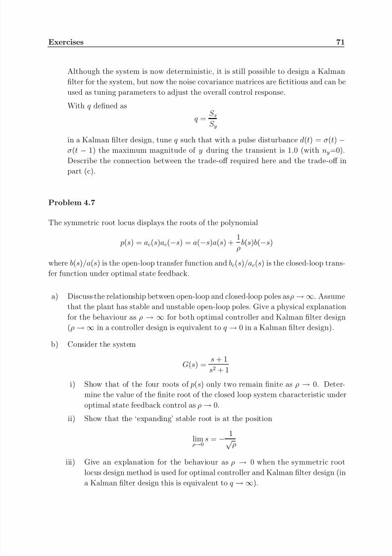
7/28/2019 Control System Theory and Design
http://slidepdf.com/reader/full/control-system-theory-and-design 79/290
Exercises 71
Although the system is now deterministic, it is still possible to design a Kalman
filter for the system, but now the noise covariance matrices are fictitious and can be
used as tuning parameters to adjust the overall control response.
With q defined as
q =S xS y
in a Kalman filter design, tune q such that with a pulse disturbance d(t) = σ(t) −σ(t − 1) the maximum magnitude of y during the transient is 1.0 (with ny=0).
Describe the connection between the trade-off required here and the trade-off in
part (c).
Problem 4.7
The symmetric root locus displays the roots of the polynomial
p(s) = ac(s)ac(−s) = a(−s)a(s) +1
ρb(s)b(−s)
where b(s)/a(s) is the open-loop transfer function and bc(s)/ac(s) is the closed-loop trans-
fer function under optimal state feedback.
a) Discuss the relationship between open-loop and closed-loop poles as ρ → ∞. Assume
that the plant has stable and unstable open-loop poles. Give a physical explanation
for the behaviour as ρ → ∞ for both optimal controller and Kalman filter design
(ρ → ∞ in a controller design is equivalent to q → 0 in a Kalman filter design).
b) Consider the system
G(s) =s + 1
s2 + 1
i) Show that of the four roots of p(s) only two remain finite as ρ→
0. Deter-
mine the value of the finite root of the closed loop system characteristic under
optimal state feedback control as ρ → 0.
ii) Show that the ‘expanding’ stable root is at the position
limρ→0
s = − 1√ ρ
iii) Give an explanation for the behaviour as ρ → 0 when the symmetric root
locus design method is used for optimal controller and Kalman filter design (in
a Kalman filter design this is equivalent to q → ∞).

7/28/2019 Control System Theory and Design
http://slidepdf.com/reader/full/control-system-theory-and-design 80/290
72 4. Observer-Based Control
Problem 4.8
Consider again the polynomial p(s) of Problem 4.7. Let
a(s) = sn + an−1sn−1 + . . . + a0
b(s) = bmsm + bm−1sm−1 + . . . + b0
where m < n, and assume ρ → 0.
a) Show that P (s) = ac(s)ac(−s) has 2m finite roots. What are their locations?
b) Show that for large values of s the roots of the polynomial p(s) tend towards the
roots of
(−1)ns2n +1
ρ(−1)mb2ms2m = 0
Hint: For large s, you can assume that a(s) ≈ sn and b(s) ≈ bmsm
d) Show that in general the roots are complex with magnitudes
|s| = r =
b2mρ
12(n−m)
e) For n − m = 1 show that the infinite root of ac(s) is −r.
f ) For n − m = 2 show that the infinite roots of ac(s) are 1√ 2
r(−1 ± j)
Problem 4.9
Consider a system with transfer function
G(s) =b(s)
a(s)
a) Assume that the symmetric root locus polynomial p(s) has a root on the imaginary
axis. Show that this implies that
|a( jw)|2 +1
ρ|b( jw)|2 = 0
b) Show that this can only be true if a(s) and b(s) can be factored as
a(s) = a(s)(s − jω0)
b(s) = b(s)(s − jω0)

7/28/2019 Control System Theory and Design
http://slidepdf.com/reader/full/control-system-theory-and-design 81/290
Exercises 73
c) Use (b) to show that p(s) has no roots on the imaginary axis if the system is
stabilizable and detectable.
Hint: Show that there is a contradiction between the symmetric root locus having roots on the imaginary axis and the plant being stabilizable and detectable.

7/28/2019 Control System Theory and Design
http://slidepdf.com/reader/full/control-system-theory-and-design 82/290
Chapter 5
Multivariable Systems
The previous chapters introduced the basic concepts of state space methods for the anal-
ysis and design of control systems; however, the discussion was limited to single-input
single-output systems. A major advantage of state space methods is the fact that multi-
input multi-output systems can be handled within the same framework. In this chapter
we will extend the concepts and results introduced so far to MIMO systems.
5.1 Transfer Function Models
As an example of a multivariable system, a simplified model of a turbogenerator is shown
in Fig. 5.1. A gas turbine is driving a synchronous generator; the gas inflow is controlled
by a servo valve (control input u1). A second control input (u2) is the adjustable excitation
current. Measured outputs are the turbine speed (y1) and the rectified voltage across a
symmetric load (y2).
Each control input has an effect on both measured outputs. Assuming that the plant
behaviour has been linearized about a given operating point, a dynamic model of this
system includes four linear sub-models, describing the dynamics from each input to each
output, i.e. gas inflow → turbine speed, gas inflow → output voltage, excitation current →turbine speed and excitation current → output voltage. If both turbine speed and output
voltage are to be controlled independently, then an efficient control strategy should take
each of these four sub-models into account. A compact way of representing the overall
dynamics of the plant is to collect input and output signals into an input and an output
signal vector, respectively. A transfer function model can then be written asY 1(s)
Y 2(s)
=
G11(s) G12(s)
G21(s) G22(s)
U 1(s)
U 2(s)
where each linear sub-model is represented by a single-input single-output transfer func-
tion model Gij(s).

7/28/2019 Control System Theory and Design
http://slidepdf.com/reader/full/control-system-theory-and-design 83/290
5.1. Transfer Function Models 75
excitationcurrent
servovalve
y1
u1 u2
turbine
load
tachogenerator
synchronousgenerator
symmetric
y2
GT
Figure 5.1: Turbogenerator
Multivariable systems can be inerconnected in the same way as single-input single-output
systems. Care must however be taken because matrix multiplication is not commutative.
For two given systems with transfer functions G1(s) and G2(s), some basic connections
are shown in Figures 5.2 - 5.4.A series connection is shown in Figure 5.2. This connection is possible if the dimensions
of y1 and u2 are equal, an equivalent system is then G2(s)G1(s). Note that in general this
is different from G1(s)G2(s), the latter product is not even defined if the dimensions of
y2 and u1 are not the same.
y1 = u2G2(s) y2u1 G1(s)
Figure 5.2: Blocks in series
Figure 5.3 shows a parallel connection. If both systems have the same number of inputs
and outputs, this connection is possible and an equivalent system is G1(s) + G2(s).
The feedback loop shown in Figure 5.4 requires that the dimensions of y1 and u2 as well
as the dimensions of y2 and u1, respectively, are the same. Solving
y1 = G1(r + G2y1)
for y1 yields
y1 = (I − G1G2)−1G1r (5.1)

7/28/2019 Control System Theory and Design
http://slidepdf.com/reader/full/control-system-theory-and-design 84/290
76 5. Multivariable Systems
u
G1(s)
G2(s)
y1
y2
y
Figure 5.3: Blocks in parallel
On the other hand, if we solve
u1 = r + G2G1u1
for u1 we obtain
y1 = G1(I − G2G1)−1r (5.2)
Note that (5.1) and (5.2) are equivalent expressions for the closed-loop system in Figure
5.4.
u1
G1(s) y1
u2
y2
G2(s)
r
Figure 5.4: Blocks in feedback
5.2 State Space Models
Recall that a multivariable state space model
x(t) = Ax(t) + Bu(t)
y(t) = Cx(t) + Du(t)
was introduced in Chapter 1, where B and D have as many columns as there are plant
inputs, and the number of rows of C and D equals the number of plant outputs. For
strictly proper systems we have D = 0.
An experimentally identified state space model of a turbogenerator plant as described
above is introduced and explored in Exercise 5.3. We will now discuss the conversion

7/28/2019 Control System Theory and Design
http://slidepdf.com/reader/full/control-system-theory-and-design 85/290
5.2. State Space Models 77
between transfer function models and state space models of multivariable systems. Given
a state space model, it is straightforward to check - just as in the SISO case discussed in
Chapter 1 - that the associated transfer function is
G(s) = C (sI − A)−1B + D (5.3)
Obtaining a state space model from a given transfer function matrix is less straightforward,
this will be illustrated by an example.
Example 5.1
Consider a plant with two inputs and two outputs, that can be described by the transfer
function matrix
G(s) = 1
s+1
2
s+1−1
(s+1)(s+2)1
s+2
(5.4)
As a first attempt to construct a state space realization of this model, we combine the
state space models (Aij, bij, cij) of the four SISO transfer functions Gij(s) to obtain the
MIMO model. Controller forms of the four sub-models can be written down by inspection
as
G11(s) → (−1, 1, 1)
G12(s) → (−1, 1, 2)
G21(s) → 0 1−2 −3
,0
1
, [−1 0]
G22(s) → (−2, 1, 1)
These four models can be arranged as
x =
A11 0
A12
A21
0 A22
x +
b11 0
0 b12b21 0
0 b22
u1
u2
y1y2
=c11 c12 0 0
0 0 c21 c22
x
yielding the MIMO state space model
x =
−1 0 0 0 0
0 −1 0 0 0
0 0 0 1 0
0 0 −2 −3 0
0 0 0 0 −2
x +
1 0
0 1
0 0
1 0
0 1
u1
u2
y1y2
=1 2 0 0 0
0 0 −1 0 1
x (5.5)

7/28/2019 Control System Theory and Design
http://slidepdf.com/reader/full/control-system-theory-and-design 86/290
78 5. Multivariable Systems
The state vector of the MIMO model contains five state variables - the state variables
of each sub-model; the order of the MIMO model equals the sum of the orders of the
sub-models. One can check that substituting the matrices (A,B,C ) of this model in (5.3)
yields indeed the transfer function matrix (5.4).
5.3 The Gilbert Realization
We will now present a different way of finding a state space realization of a transfer func-
tion model, known as Gilbert realization . This realization is only possible if all eigenvalues
of the model are distinct, i.e. if no sub-model has repeated eigenvalues. The idea is as
follows. First, a transfer function matrix G(s) can be rewritten as
G(s) =1
d(s)N (s)
where the least common multiple d(s) of all denominator polynomials has been pulled
out as a common factor, leaving a “numerator” polynomial matrix N (s). Assuming deg
d(s) = r, a partial fraction expansion is
G(s) =N 1
s − λ1
+N 2
s − λ2
+ . . . +N r
s − λr
where the residuals N i can be computed elementwise. Defining
ρi = rank N i
each residual matrix N i can be factored as
N i = C iBi, C i ∈ IRl×ρi, Bi ∈ IRρi×m
Now each term in the partial fraction expansion can be written as
N is
−λi
= C i1
s
−λi
Bi = C i(sI ρi − λiI ρi)−1Bi
where I ρi denotes the ρi × ρi identity matrix. Thus we obtain for each term a state space
realizationN i
s − λi→ (Ai, Bi, C i)
where Ai = λiI ρi . A combination of these terms by forming a parallel connection yields a
MIMO state space model
x =
λ1I ρ1 0
. . .
0 λrI ρr
x +
B1
...
Br
u
y = [C 1 . . . C r]x

7/28/2019 Control System Theory and Design
http://slidepdf.com/reader/full/control-system-theory-and-design 87/290
5.4. Controllability and Observability 79
This realization of G(s) has ρ =r
i=1 ρi state variables.
Example 5.1 (continued)To obtain the Gilbert realization of the model (5.4), we rewrite G(s) as
G(s) =1
d(s)N (s) =
1
(s + 1)(s + 2)
s + 2 2(s + 2)
−1 s + 1
and compute the partial fraction expansion as
G(s) =1
s + 1
1 2
−1 0
+
1
s + 2
0 0
1 1
We have ρ1 = 2, ρ2 = 1. Factorizing N 1 and N 2 as
N 1 = C 1B1 =
1 0
0 1
1 2
−1 0
, N 2 = C 2B2 =
0
1
[1 1]
we obtain the MIMO model
x =
−1 0 0
0 −1 0
0 0 −2
x +
1 2
−1 0
1 1
u1
u2
y1y2
=
1 0 0
0 1 1
x (5.6)
This realization of G(s) in Example 5.1 has three state variables, two less than the realiza-
tion in (5.5). However, it is straightforward to check that substituting the matrices of this
model in (5.3) yields the same transfer function. From the discussion in Chapter 3, we
would therefore expect that at least two state variables in (5.5) are either uncontrollable
or unobservable. This is indeed the case, but before we can establish this, we need to
extend the concepts of controllability and observability to MIMO systems.
5.4 Controllability and Observability
We will now extend the results of Chapters 2 and 3 to MIMO systems. Consider a system
with state space realization
x(t) = Ax(t) + Bu(t)
y(t) = Cx(t) + Du(t) (5.7)
where x(t) ∈ IRn, u(t) ∈ IRm, y(t) ∈ IRl, and the matrices (A,B,C,D) are of compatible
dimensions.

7/28/2019 Control System Theory and Design
http://slidepdf.com/reader/full/control-system-theory-and-design 88/290
80 5. Multivariable Systems
Definition 5.1
The system (5.7) is said to be controllable if for any initial state x(0) = x0, time tf > 0
and final state xf there exists a control input u(t), 0 ≤ t ≤ tf , such that the solution of
(5.7) satisfies x(tf ) = xf . Otherwise, the system is said to be uncontrollable.
The following can be shown in a way similar to the proofs of the corresponding SISO
results in Chapter 2.
Theorem 5.1
The following statements are equivalent:
(i) The system (5.7) is controllable.
(ii) The controllability Gramian
W c(t) =
t
0
eAτ BB T eAT τ dτ
is positive definite for any t > 0.
(iii) The controllability matrix
C(A, B) = [B AB . . . An−1B]
has full row rank.
(iv) The matrix
[sI − A B]
has full row rank for all s
∈|C.
Notice that in contrast to SISO systems where the controllability matrix C(A, b) is a n×n
square matrix, the controllability matrix C(A, B) of a MIMO system is n × mn, i.e. it has
more columns than rows. But just as for SISO systems, rank C(A, B) = n (full row rank)
ensures that the controllable subspace - the column space of C(A, B) - is the whole state
space. It is possible that the partial controllability matrix
Cr(A, B) = [B AB . . . Ar−1B]
where r < n, has rank n. In this case the smallest integer ν c for which rank Cν c(A, B) = n
is called the controllability index of the system (A, B).

7/28/2019 Control System Theory and Design
http://slidepdf.com/reader/full/control-system-theory-and-design 89/290
5.4. Controllability and Observability 81
Definition 5.2
The system (5.7) is said to be observable if for any tf > 0 the initial state x(0) can be
uniquely determined from the time history of the input u(t) and the output y(t) in the
time interval 0 ≤ t ≤ tf . Otherwise, the system is said to be unobservable.
Theorem 5.2
The following statements are equivalent:
(i) The system (5.7) is observable.
(ii) The observability Gramian
W o(t) =
t
0
eAT τ C T CeAτ dτ
is positive definite for any t > 0.
(iii) The observability matrix
O(C, A) = C
CA...
CAn−1
has full column rank.
(iv) The matrix sI − A
C
has full column rank for all s
∈|C.
The proof of Theorem 3.2 (the SISO version of the statement (iii) ⇔ (i) in Theorem 5.2)
was based on the fact that the equation
Y = O(c, A)x(0)
where Y is a column vector containing y(0), y(0) etc., can be solved uniquely for x(0)
if the observability matrix O(c, A) has full rank. For MIMO systems the observability
matrix is ln
×n, i.e. it has more rows than columns. However, multiplying the above from
the right by OT leads to
x(0) = (OT O)−1OT Y
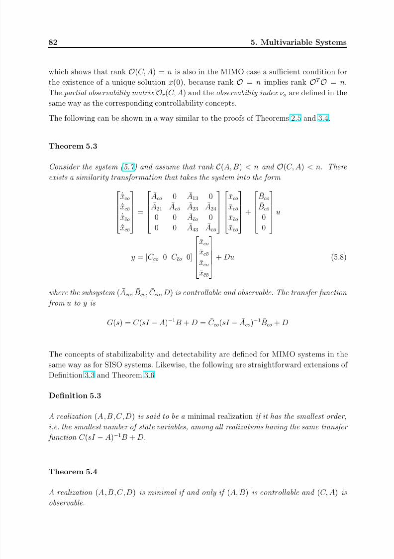
7/28/2019 Control System Theory and Design
http://slidepdf.com/reader/full/control-system-theory-and-design 90/290
82 5. Multivariable Systems
which shows that rank O(C, A) = n is also in the MIMO case a sufficient condition for
the existence of a unique solution x(0), because rank O = n implies rank OT O = n.
The partial observability matrix O
r(C, A) and the observability index ν o are defined in the
same way as the corresponding controllability concepts.
The following can be shown in a way similar to the proofs of Theorems 2.5 and 3.4.
Theorem 5.3
Consider the system (5.7) and assume that rank C(A, B) < n and O(C, A) < n. There
exists a similarity transformation that takes the system into the form
˙xco
˙xco
˙xco
˙xco
=
Aco 0 A13 0A21 Aco A23 A24
0 0 Aco 0
0 0 A43 Aco
xco
xco
xco
xco
+
Bco
Bco
0
0
u
y = [C co 0 C co 0]
xco
xco
xco
xco
+ Du (5.8)
where the subsystem (Aco, Bco, C co, D) is controllable and observable. The transfer function from u to y is
G(s) = C (sI − A)−1B + D = C co(sI − Aco)−1Bco + D
The concepts of stabilizability and detectability are defined for MIMO systems in the
same way as for SISO systems. Likewise, the following are straightforward extensions of
Definition 3.3 and Theorem 3.6
Definition 5.3
A realization (A,B,C,D) is said to be a minimal realization if it has the smallest order,
i.e. the smallest number of state variables, among all realizations having the same transfer
function C (sI − A)−1B + D.
Theorem 5.4
A realization (A,B,C,D) is minimal if and only if (A, B) is controllable and (C, A) is
observable.

7/28/2019 Control System Theory and Design
http://slidepdf.com/reader/full/control-system-theory-and-design 91/290
5.4. Controllability and Observability 83
Returning to Example 5.1 and its Gilbert realization, it turns out that (5.3) is a minimal
realization, because - as shown in Exercise 5.9 - a Gilbert realization is always controllable
and observable.
Multivariable Poles and Zeros
A linear system is stable if all its poles are strictly inside the left half of the complex
plane. So far we have not yet extended the concept of poles and zeros to multivariable
systems. As Example 5.1 indicated, it may not be trivial to determine what the poles
of a multivariable system are. Clearly, in that example we can say by inspection of the
transfer function matrix that the poles are located at s = −1 and s = −2. What is
however not immediately clear is the multiplicity of the poles at these locations. Exactly
how many poles the system has at each of these locations plays for example a role when
a multivariable version of the Nyquist stability criterion is used to assess the closed-loop
stability of a control system. At first glance, it is not even clear how many poles the
system has at all - to answer that question we need to know the degree of its minimal
realization.
We will define poles of a multivariable system in terms of a minimal state space realization.
Let (A,B,C,D) be a realization of G(s), and recall that
G(s) =C adj(sI
−A)B
det(sI − A) + D
The numerator C adj(sI − A)B is a polynomial matrix, and it is clear that every pole
of G(s) must be a zero of det (sI − A) (i.e. an eigenvalue of A). However, not every
zero of det (sI − A) needs to be a pole (because there may be cancellations by zeros in
the numerator that occur in all subsystems). If this happens, the realization is either
uncontrollable or unobservable, which motivates the following definition.
Definition 5.4
Let (A,B,C,D) be a minimal realization of a system with transfer function matrix G(s).The eigenvalues of A are called the poles of G(s).
In Section 4.2 we introduced the distinction between invariant zeros and transmission
zeros.
Definition 5.5
Let (A,B,C,D) be a realization of G(s). G(s) has an invariant zero at z i if z i satisfies
detz iI − A −B
C D
= 0.

7/28/2019 Control System Theory and Design
http://slidepdf.com/reader/full/control-system-theory-and-design 92/290
84 5. Multivariable Systems
Definition 5.6
G(s) has a transmission zero at z i if there exists a vector u0
= 0 such that G(z i)u0 = 0.
Recall from Section 4.2 that if a state space realization is minimal, invariant and trans-
mission zeros are the same, but if a realization has uncontrollable or unobservable modes,
then there will be invariant zeros that do not appear as transmission zeros.
Multivariable poles and zeros are usually defined in terms of the Smith-McMillan form of
a system which is discussed in the next section. One can prove that the poles according
to Definition 5.4 and the transmission zeros according to Definition 5.6 are the same as
those defined in terms of the Smith-McMillan form.
5.5 The Smith-McMillan Form
We will now introduce an alternative definition of multivariable poles and zeros. Consider
again the system of Example 5.1. The transfer function is
G(s) =
1
s+12
s+1
−1(s+1)(s+2)
1s+2
=
1
(s + 1)(s + 2)
s + 2 2(s + 2)
−1 s + 1
=
1
d(s)N (s)
where d(s) is the least common multiple of all denominator polynomials. Obviously, the
poles of this system should be defined such that the poles of the individual elements of
G(s) are included; what is less obvious is with what multiplicity these poles - at s = −1
and s = −2 in the above example - should be counted as poles of the MIMO system. Even
less obvious are the zeros of this system. The multivariable poles and zeros are usually
defined in terms of a diagonal canonical form to which every transfer function matrix can
be reduced, known as the Smith-McMillan form .
The Smith-McMillan FormTo introduce the Smith-McMillan form, we start with the factorization G(s) = N (s)/d(s),
where N (s) is a polynomial matrix and d(s) the least common multiple of the denomi-
nators. The following Theorem states that every polynomial matrix can be transformed
into a special diagonal form by elementary row or column operations. (Elementary row
or column operations are the interchange of two rows or columns, and the addition of a
polynomial multiple of a row or column to another.)
Theorem 5.5
A polynomial matrix N (s) of dimension l × m can always be transformed by a sequence

7/28/2019 Control System Theory and Design
http://slidepdf.com/reader/full/control-system-theory-and-design 93/290
5.5. The Smith-McMillan Form 85
of elementary column and row operations into the form
Λ(s) =
β 1(s) 0
. . .
β r(s)
0 0
(5.9)
where the β i(s) are unique monic polynomials (i.e. the highest power of s has coefficient
1) such that β i(s) | β i+1(s) ( β i(s) divides β i+1(s) without remainder) for i = 1, . . . , r, and
r is the rank of N (s) for almost all s.
The matrix Λ(s) is known as the Smith form of N (s). To prove the Theorem, we outline
how the Smith form can be constructed. By interchange of columns and rows, bring theelement of N (s) with least degree to the (1,1) position. Use elementary row operations
to make all entries in the first column below the (1,1) entry zero. Use elementary column
operations to make all entries in the first row except the (1,1) entry zero. These column
operations may bring back non-zero elements to the first column. In this case repeat the
above steps until all elements of row 1 and column 1 are zero except the (1,1) entry. This
yields a matrix of the form β 1(s) 0
0 N 1(s)
where β 1(s) divides every element of N 1(s). Repeat the whole procedure on N 1(s). Pro-ceeding in this way leads to the Smith form Λ(s) of N (s).
We will say that N (s) is similar to Λ(s) and use the notation N (s) ∼ Λ(s). Now returning
to the factorization
G(s) =1
d(s)N (s)
of a transfer function matrix, it follows that
G(s) ∼1
d(s) Λ(s) = β 1(s)α1(s)
0. . .
β r(s)αr(s)
0 0
(5.10)
where β i(s) | β i+1(s) and αi+1(s) | αi(s). This form of a transfer function matrix is called
the Smith-McMillan form.
Definition 5.7
Consider a transfer function matrix G(s) and its Smith-McMillan form as in (5.10).
Introduce the polynomials
β (s) = β 1(s)β 2(s) . . . β r(s), α(s) = α1(s)α2(s) . . . αr(s) (5.11)

7/28/2019 Control System Theory and Design
http://slidepdf.com/reader/full/control-system-theory-and-design 94/290
86 5. Multivariable Systems
The roots of the polynomials β (s) and α(s) are called the zeros and poles of G(s), respec-
tively. The degree of α(s) is called the McMillan degree of G(s).
It is clear from the above definition that the poles of G(s) include all poles of its individual
entries. Moreover, the Smith-McMillan form determines the multiplicity of each pole. The
McMillan degree is equal to the number of poles. It can be shown that the poles of G(s) in
the sense of Definition 5.7 are the eigenvalues of the state matrix of a minimal realization.
This also implies that the McMillan degree of G(s) is the order of its minimal realization.
Returning to the system of Example 5.1, we find that (see Exercise 5.6)
G(s) = 1
s+12
s+1
−1(s+1)(s+2)
1s+2
∼ − 1
(s+1)(s+2)0
0 s+3s+1
Thus, the poles are -1, -1 and -2. These are exactly the eigenvalues of the Gilbert re-
alization, and the order of the Gilbert realization is equal to the McMillan degree. The
system also has a zero at s = −3. This zero is not obvious from the transfer function
matrix G(s), but we have
G(−3) =
−12
−1
−12
−1
so -3 is a value of s where G(s) loses its full rank. The significance of such multivariable
zeros is illustrated in Exercises 5.11 and 5.12, where it is shown that a multivariableright-half-plane zero has an effect similar to a right-half-plane zero of a SISO system.
5.6 Multivariable Feedback Systems and Closed-Loop
Stability
In this section we introduce a multivariable feedback structure and discuss its stability.
Well-Posedness of a Feedback Loop
Consider the feedback loop in Figure 5.5. For given proper transfer functions G1(s) and
G2(s), we might first want to check whether the closed-loop transfer function is proper.
That this may not always be the case is illustrated by the following example. Let
G1(s) = 1, G2(s) =s − 2
s + 3
Even though both transfer functions are proper, we have
e2 =
s + 3
5 (u1 + u2)
Thus, the transfer function from u1 to e2 is not proper.

7/28/2019 Control System Theory and Design
http://slidepdf.com/reader/full/control-system-theory-and-design 95/290
5.6. Multivariable Feedback Systems and Closed-Loop Stability 87
Definition 5.8 A feedback loop is well-posed if all closed-loop transfer functions are
proper.
One can show that if either G1(s) or G2(s) is strictly proper, the feedback loop in Figure
5.5 is well-posed. From now on we will assume that the feedback loops we consider are
well-posed.
e1G1(s)u1
G2(s) u2
e2
Figure 5.5: Feedback loop
Internal Stability
Assume we want to check the stability of the closed-loop transfer function from u1 to
the output of G1 in Figure 5.5. In the case of single-input single-output systems, the
closed-loop transfer function from u1 to the output of G1 is
G1(s)1 − G1(s)G2(s)
To check stability we could investigate the zeros of the denominator 1 − G1G2 - this is in
fact what we do when we apply the Nyquist stability test or root locus techniques. Again,
a simple example illustrates that we need to be careful.
Example 5.2
Let
G1(s) =1
s − 1, G2(s) =
s − 1
s + 2We can check that
1 − G1(s)G2(s) =s + 1
s + 2
which has no zeros in the right half plane. However, the closed-loop transfer function is
G1(s)
1 − G1(s)G2(s)=
s + 2
(s + 1)(s − 1)
which is unstable. The problem here is that an unstable pole-zero cancellation prevents
the unstable closed-loop pole from being detected. One might ask why this issue has not
been raised when the Nyquist stability test for SISO systems was introduced. The answer
is that when using classical design techniques for SISO systems, one can asssume that the

7/28/2019 Control System Theory and Design
http://slidepdf.com/reader/full/control-system-theory-and-design 96/290
88 5. Multivariable Systems
designer has explicit control over pole and zero locations and will usually avoid unstable
pole-zero cancellations. For MIMO systems, automated design techniques are often used
to find a controller, and in some cases internal stability must be checked.
We now turn to MIMO systems and allow u1, u2, e1 and e2 to be vector signals. Again
we want to check whether the feedback loop in Figure 5.5 is internally stable. Define the
transfer functions H ij(s), i = 1, 2 bye1e2
=
H 11 H 12H 21 H 22
u1
u2
Definition 5.9
The feedback system in Figure 5.5 is called internally stable if and only if the transfer function matrix
H 11(s) H 12(s)
H 21(s) H 22(s)
is stable.
This definition makes sure that no unstable pole-zero cancellation prevents an unstable
closed-loop pole from being detected. Note that internal stability requires that each of
the four transfer matrices H ij(s) is stable.
One can show that the feedback loop is internally stable if and only if
(i) there is no unstable pole-zero cancellation in G1(s)G2(s), and
(ii) the transfer function (I − G1(s)G2(s))−1 is stable.
Now introduce
φ(s) = det(I
−G1(s)G2(s))
and note that (ii) is equivalent to φ(s) having all its zeros in the open left half plane. With
these results we can now formulate a MIMO version of the Nyquist stability criterion. Let
n1 be the number of unstable poles of G1(s) and n2 the number of unstable poles of G2(s).
Observing that φ(s) has all zeros in the open left half plane if and only if the Nyquist plot
of φ( jω) encircles the origin n1 + n2 times counter-clockwise, we conclude the following.
Theorem 5.6 The feedback loop in Figure 5.5 is internally stable if and only if
(i) there is no pole-zero cancellation in G1(s)G2(s)
(ii) the Nyquist plot of φ( jω) encircles the origin n1 + n2 times counter-clockwise.

7/28/2019 Control System Theory and Design
http://slidepdf.com/reader/full/control-system-theory-and-design 97/290
5.7. A Multivariable Controller Form 89
5.7 A Multivariable Controller Form
We will now extend the idea used in Section 1.1 for the construction of the controller formstate space realization to multivariable systems. The resulting multivariable controller
form will be the basis for a discussion of multivariable pole placement in the following
section.
In the SISO case, the starting point for the construction of a state space model from a
transfer function was the factorization of the transfer function model shown in Fig. 1.3.
For a l × m MIMO transfer function model G(s), we now introduce the factorization
G(s) = N (s)D−1(s) (5.12)
where N (s) is a l×m and D(s) a m×m polynomial matrix. Such a representation is calleda (right) matrix fraction description (MFD) of G(s) (a left matrix fraction description is
G(s) = D−1(s)N (s)). An MFD of G(s) is not unique, one choice is to start with the
factorization G(s) = N (s)/d(s) that was used for the Gilbert realization, and to define
D(s) = d(s)I . Other MFDs can be generated by multiplying G(s) from the right by a
polynomial matrix D(s) which is chosen such that all denominator polynomials in G(s)
are cancelled, leading to G(s)D(s) = N (s) where N (s) is a polynomial matrix.
We will now illustrate the construction of a multivariable controller form with an example.
Example 5.3
Consider a plant with transfer function model
G(s) =
s
(s+1)2(s+2)2s
(s+2)2
−s(s+2)2
−s(s+2)2
(5.13)
An MFD of this plant is
G(s) = s 0
−s s2
0 −(s + 1)2(s + 2)
(s + 2)2
s + 2 −1
(5.14)
To follow the development in Section 1.1, we introduce the representation shown in Fig.
5.6 (the MIMO equivalent of Fig. 1.3), where the m-dimensional signal vector v(t) is
introduced as the output of the multivariable filter D−1(s). In the SISO case, the idea was
to express input and output signal in terms of v(t), to assume that the highest derivative
of this signal (determined by the highest power of s in a(s)) is somehow available and
then to generate it by using a chain of integrators. To do something similar for a MIMO
system, we first need the equivalent of the highest derivative of v(t). Now v(t) is a signal
vector, and we should consider the highest powers of s in D(s). We will do this by writing
D(s) as
D(s) = DhS (s) + DlΨ(s) (5.15)

7/28/2019 Control System Theory and Design
http://slidepdf.com/reader/full/control-system-theory-and-design 98/290
90 5. Multivariable Systems
where
S (s) =
s2 0
0 s3D−1(s)u(t) N (s) y(t)
v(t)
Figure 5.6: Matrix fraction description of plant model
is a diagonal matrix that has the highest power of s in each column of D(s) as element in
the corresponding position, Ψ(s) contains the lower powers of s, and Dh and Dl are the
coefficient matrices for the highest and the lower powers of s, respectively. For the MFD
in (5.14) this decomposition is
D(s) =
0 −(s + 1)2(s + 2)
(s + 2)2 s + 2
=
0 −s3 − 4s2 − 5s − 2
s2 + 4s + 4 s + 2
=
0 −1
1 0
s2 0
0 s3
+
0 0 −4 −5 −2
4 4 0 1 2
s 0
1 0
0 s2
0 s
0 1
= DhS (s) + DlΨ(s)
The next step is to generate v(t) by repeatedly integrating the highest derivatives of each
element of this signal vector. We have
U (s) = D(s)V (s) = DhS (s)V (s) + DlΨ(s)V (s) (5.16)
thus
S (s)V (s) = −D−1h DlΨ(s)V (s) + D−1
h U (s) (5.17)
Equation (5.16) is the MIMO equivalent of (1.12) in the SISO case, where the plant model
was normalized such that the characteristic polynomial a(s) is monic. The assumptionthat Dh is invertible corresponds in the scalar case to the assumption that a(s) is indeed
a polynomial of degree n (i.e. an = 0). Because
S (s)V (s) =
s2 0
0 s3
V 1(s)
V 2(s)
→
v1(t)...v 2(t)
and
Ψ(s)V (s) =
s 0
1 0
0 s2
0 s
0 1
V 1(s)
V 2(s) →
v1(t)
v1(t)
v2(t)
v2(t)
v2(t)

7/28/2019 Control System Theory and Design
http://slidepdf.com/reader/full/control-system-theory-and-design 99/290
5.7. A Multivariable Controller Form 91
the vector S (s)V (s) represents the highest derivatives of each element of v(t), whereas
Ψ(s)V (s) collects all lower derivatives. We can now proceed in the same way as in the
SISO case: we assume temporarily that the highest derivative of each element of v(t)
is available, and integrate repeatedly to obtain all lower derivatives. Instead of a single
integrator chain, we need however m integrator chains. The outputs of the integrators
are the entries of Ψ(s)V (s), which can be used for feedback through the gain matrix
D−1h Dl and added to D−1
h U (s) to generate the vector S (s)V (s), according to (5.17). Like
in (1.13) for SISO systems, the output vector Y (s) can be obtained as a weighted sum of
the elements of Ψ(s)V (s): from Fig. 5.6 we have
Y (s) = N (s)V (s) = N lΨ(s)V (s)
where N l is the coefficient matrix of N (s). This leads to the model in Fig. 5.7, which is
a multivariable version of Fig. 1.4. A controllable state space realization of this model is
developed in Exercise 5.13.
−
Ψv
v1
v2
D−1h Sv
v2
v1 v2
v1
N l
...v2
D−1h Dl
u
y
Ψv
Figure 5.7: Time-domain model of G(s)
For reasons that will become clear when pole placement by state feedback around this
realization is discussed in the next section, we will call this realization a multivariable con-
troller form . In the scalar case, we called the equivalent realization a canonical controller
form, reflecting the fact that for a SISO system, the procedure described in Section 1.1
leads to a unique realization. This is not the case for a MIMO system: the model in Fig.
5.7 depends on the choice of MFD (in the given example on (5.14)), which is not unique.
Because different MFDs will lead to different controller forms of the same system, this
multivariable controller form is not called a canonical realization.

7/28/2019 Control System Theory and Design
http://slidepdf.com/reader/full/control-system-theory-and-design 100/290
92 5. Multivariable Systems
5.8 Pole Placement
We will now develop a multivariable version of the pole placement technique that wasused in Exercise 1.7. In the previous section we saw that a multivariable controller form
can be constructed from an MFD
G(s) = N (s)D−1(s)
where D(s) is chosen such that its highest coefficient matrix Dh in (5.15) has full rank.
Referring to the model in Fig. 5.7, it is clear that the state variables of this system are
completely determined by the signal vector Ψ(s)V (s). We can therefore represent state
feedback through a gain matrix F as shown in Fig. 5.8. From Fig. 5.8, the closed-loop
transfer function isGF (s) =
Y (s)
U v(s)= N (s)D−1
F (s)
We have
U (s) = D(s)V (s) = U v(s) + F Ψ(s)V (s)
thus
U v(s) = (D(s) − F Ψ(s))V (s) = DF (s)V (s)
which shows that
DF (s) = D(s) − F Ψ(s) (5.18)and after substituting from (5.15)
DF (s) = DhS (s) + (Dl − F )Ψ(s) (5.19)
D−1F (s)
Ψ(s)
D−1(s)
F
uuv N (s) y
v
x
Figure 5.8: State feedback for multivariable controller form
This should be compared with the observation made in Exercise 1.7, that for a SISO
model under state feedback around a controller form realization (Ac, bc, cc) we have
det(sI − Ac − bcf ) = sn + (an−1 − f n)sn−1 + (an−2 − f n−1)sn−2 + . . . + (a0 − f 1)

7/28/2019 Control System Theory and Design
http://slidepdf.com/reader/full/control-system-theory-and-design 101/290
5.8. Pole Placement 93
where
det(sI − A) = sn + an−1sn−1 + . . . + a0
is the open-loop characteristic polynomial. All coefficients (except for the highest power of s) of the closed-loop polynomial can be assigned arbitrary values by the appropriate choice
of the state feedback gains f i, therefore the closed-loop eigenvalues can be arbitrarily
chosen. From (5.19) we see that the same is true for MIMO systems: by choosing the
gain matrix F we can arbitrarily change all coefficients in D(s) except for the highest
powers in each column. We would therefore expect that by choice of F we can obtain any
desired closed-loop polynomial. This is indeed the case, and we will derive a procedure
for computing a gain matrix F that achieves this. We also observe that - just as we found
for SISO systems - state feedback does not alter the numerator polynomial matrix N (s).
An Eigenvector Method for Pole Placement
We will now assume that the plant is represented by a state space model in the controller
form (Ac, Bc, C c) developed in Exercise 5.13 from Fig. 5.7. Thus assume that the plant
dynamics are governed by the state equation
x(t) = Acx(t) + Bcu(t)
and state feedback u(t) = F x(t) is to be used to assign a set of distinct closed-loop
eigenvalues λ1, λ2, . . . , λn. These closed-loop eigenvalues are the solutions of
det DF (s) = 0
We will also need the closed-loop eigenvectors , i.e. the vectors hi, i = 1, . . . , n that satisfy
(Ac + BcF )hi = λihi
It can be shown that the eigenvectors hi can be expressed as
hi = Ψ(λi) pi
where pi is any vector in the nullspace of DF (λi), i.e. a vector such that
DF (λi) pi = 0
(this is illustrated in Exercise 5.14.) Now from (5.18) it follows that
D(λi) pi − F Ψ(λi) pi = 0
Defining the vectors gi = D(λi) pi, i = 1, . . . , n, we thus have
F hi = gi, i = 1, . . . , n
or
F [h1 . . . hn] = [g1 . . . gn]

7/28/2019 Control System Theory and Design
http://slidepdf.com/reader/full/control-system-theory-and-design 102/290
94 5. Multivariable Systems
Because the eigenvalues are assumed distinct, the eigenvectors are linearly independent
and we can solve for the state feedback gain
F = [g1 . . . gn][h1 . . . hn]−1 (5.20)
If the desired eigenvalues are not distinct, one can use generalized eigenvectors to obtain
a unique solution F to the pole placement problem.
The discussion leading to (5.20) shows that not only the closed-loop eigenvalues, but -
within limits - also the closed-loop eigenvectors can be assigned by state feedback. The
procedure can be summarized as follows.
1. Choose distinct closed-loop eigenvalues λ1, . . . , λn.
2. Choose closed-loop eigenvectors h1, . . . , hn such that
hi ∈ R(Ψ(λi)), i = 1, . . . , n (5.21)
and such that eigenvectors associated with a complex conjugate eigenvalue pair are
also a complex conjugate pair. With this choice, there exist vectors pi such that
hi = Ψ(λi) pi, i = 1, . . . , n.
3. Define gi = D(λi) pi, i = 1, . . . , n.
4. Compute the state feedback gain matrix F from (5.20). This gain matrix satisfies
(Ac + BcF )hi = λihi, i = 1, . . . , n
Step 2 of this procedure indicates that a given set of closed-loop eigenvalues does not
uniquely determine the state feedback gain, but that we can choose the closed-loop eigen-
vectors as well - subject to the constraint (5.21). Recall that for SISO systems equation
(2.9) shows that the solution to the pole placement problem is unique. For MIMO systems,
the additional degree of freedom can be exploited to find a solution that improves certain
performance measures. One way of choosing closed-loop eigenvalues and eigenvectors isbriefly outlined next.
5.9 Optimal Control of MIMO Systems
We will now extend the symmetric root locus design introduced in Section 4.4 to MIMO
systems. Consider a system with state space representation
x(t) = Ax(t) + Bu(t), x(0) = x0
y(t) = Cx(t)

7/28/2019 Control System Theory and Design
http://slidepdf.com/reader/full/control-system-theory-and-design 103/290
5.9. Optimal Control of MIMO Systems 95
where (A, B) is stabilizable and (C, A) is detectable. As in the SISO case, assume that
x0 = 0 and that we wish to find a control input u(t) that brings the system quickly back
to x = 0. A MIMO version of the cost function (4.12) is
V =
∞0
(yT (t)y(t) + uT (t)Ru(t))dt, R > 0
where R ∈ IRm×m is a positive definite matrix that places a cost on the control effort. A
more general form of a cost function is
V =
∞0
(xT (t)Qx(t) + uT (t)Ru(t))dt, R > 0, Q ≥ 0 (5.22)
where Q ∈ IRn×n is a positive semidefinite weighting matrix on the control error. A
common choice of weighting matrices is
Q = C T C, R =
ρ1 0
. . .
0 ρm
where Q is fixed and the ρi can be used as tuning parameters as discussed below.
Next, define the matrix
H =
A −BR−1BT
−Q −AT
(5.23)
This 2n×2n matrix plays an important role in optimal control. By applying the similaritytransformation
T =
0 I
−I 0
one can show that H is similar to −H T , which implies that if λ is an eigenvalue of H then
so is −λ. A matrix with this property is called a Hamiltonian matrix , its eigenvalues are
symmetric about the imaginary axis. For a SISO system and the choices Q = cT c and
R = ρ, one can verify that the characteristic polynomial of H is exactly the polynomial
p(s) of the symmetric root locus design, that was introduced in Section 4.4 and provides
the optimal closed-loop eigenvalues. For MIMO systems, it turns out that the Hamiltonian
matrix (5.23) provides not only the optimal eigenvalues, but also the optimal eigenvectors.
Partition the eigenvectors of H as
H
hi
gi
= λi
hi
gi
, i = 1, . . . , 2n (5.24)
where hi contains the top n entries of the 2n-dimensional eigenvectors. Assume that H
has no eigenvalues on the imaginary axis (as in the SISO case, it can be shown that
eigenvalues on the imaginary axis represent unobservable or uncontrollable modes, which
are excluded by the assumption of stabilizability and detectability). Then the optimal
control law that minimizes the cost V in (5.22) takes the form of state feedback
uopt(t) = F x(t)

7/28/2019 Control System Theory and Design
http://slidepdf.com/reader/full/control-system-theory-and-design 104/290
96 5. Multivariable Systems
and we have the following result, which is given here without proof.
Theorem 5.7
The optimal state feedback control law uopt(t) = F x(t) that minimizes the cost function
(5.22) places the eigenvalues of (A + BF ) at the stable eigenvalues of H . Moreover, the
eigenvectors of (A + BF ) are the partitions hi of the eigenvectors of H that are associated
with the stable eigenvalues.
Theorem 5.7 can be combined with the formula (5.20) to solve an optimal pole placement
problem: compute the stable eigenvalues and eigenvectors of H , and use (5.20) to compute
the optimal state feedback gain F . With the choice of weighting functions Q = C T C andR = diag (ρ1, . . . , ρm), the tuning parameters ρi can be used to trade control performance
against control effort in each input channel independently. This is illustrated in Exercise
5.10 for the turbogenerator design problem.
Optimal State Estimation
For a multivariable version of the method for optimal state estimation in Section 4.4, we
extend the deterministic state space model to
x(t) = Ax(t) + Bu(t) + w(t)y(t) = Cx(t) + v(t)
where w(t) and v(t) are white noise processes: the n-dimensional vector w(t) represents
process noise, and the l-dimensional vector v(t) measurement noise. As before, both noise
processes are assumed to be wide-sense stationary, zero-mean, Gaussian distributed and
uncorrelated, and to satisfy
E [w(t)wT (t + τ )] = Qeδ (τ ), E [v(t)vT (t + τ )] = Reδ (τ ), E [w(t)vT (t + τ )] = 0
One can show that the observer gain L that solves
minL limt→∞E [xT (t)x(t)]
i.e. that minimizes the noise power in the state estimation error, is obtained by solving
the dual version of the optimal pole placement problem, with the replacements
A, B → AT , C T
and
Q, R → Qe, Re
In practice, the noise covariance matrices are often not known explicitly, but are used as
tuning parameters. Common choices are Qe = BB T and Re = diag(r1, . . . , rl), where the
values of ri can be used to tune the speed of estimation for each output channel. This isillustrated in Exercise 5.15 for the turbogenerator design problem.

7/28/2019 Control System Theory and Design
http://slidepdf.com/reader/full/control-system-theory-and-design 105/290
Exercises 97
Exercises
Problem 5.1
Consider the plant
G(s) =1
(s + 1)(s + 5)(s + 0.1)
1 0.2
−0.1 2
a) How many characteristic loci does this plant have?
b) Write a Matlab script to determine the eigenvalues of G(s) as s takes values along
the positive and negative imaginary axis, and to draw the characteristic loci.
c) Use the plot to determine the maximum value of the constant k such that with the
controller kI in negative feedback the system remains stable.
Hint: The commands frd and frdata are useful Matlab commands for working with
multivariable frequency responses.
Problem 5.2
Consider the multivariable closed-loop system in Figure 5.9.
a) Show that the transfer function from r to e is
S = (I + GK )−1
This function is called the sensitivity function . Show that S is also the transfer
function from do to y.
b) Show that the transfer function from r to y is
T = (I + GK )−1GK = G(1 + KG)−1K = GK (I + GK )−1
This function is called the complementary sensitivity function .
c) What is the transfer function from di to ug? (This function is sometimes called the
input sensitivity function S I .) Show that GS I = SG. Note that S I = S for SISO
systems.

7/28/2019 Control System Theory and Design
http://slidepdf.com/reader/full/control-system-theory-and-design 106/290
98 5. Multivariable Systems
−
di
r e K (s) G(s)ugu y
do
Figure 5.9: Multi-variable closed loop system
Problem 5.3
Consider the state space model of an experimental turbogenerator with the followinginputs and outputs:
Input 1 (u1): Gas control valve of the turbine
Input 2 (u2): Excitation current of the generator
Output 1 (y1): Turbine speed
Output 2 (y2): Generator terminal voltage
Figure 5.10 indicates the inputs (u1, u2), the outputs (y1, y2) and the disturbances (d1,
d2) associated with the plant, G(s).
y2G(s)ug2
ug1
d1
u1
u2
d2
y1
Figure 5.10: Turbogenerator inputs, outputs and disturbances
An observer-based state feedback controller is to be designed, for this system, such that
the following operating requirements are satisfied.
i) There should be zero steady state error for:
– step changes in set points.
– step disturbances.

7/28/2019 Control System Theory and Design
http://slidepdf.com/reader/full/control-system-theory-and-design 107/290
Exercises 99
– small variations in model parameters (A,B,C,D).
ii) There should be no state estimation errors following a change in setpoint.
Matrices A, B, C and D of the plant model can be obtained from Matlab file cs5_tgen.m.
Same model will be used in problems 5.10 and 5.15 also
a) Draw the block diagram of the closed-loop system. Explain the structure of the
closed-loop system. Show the dimensions of the matrices and the signals in the
system.
b) Create the closed loop system in Simulink. Tune the pole locations of the controller
using pole placement to achieve the following setpoint tracking specifications.
i) The 5% settling time for output y1 should be less than 3.0 and the maximum
change in y2 should be less than 0.15 for step changes to setpoint r1.
ii) The 5% settling time for output y1 should be less than 2.0 and the maximum
change in y1 should be less than 0.15 for step changes to setpoint r2.
Hints:
– Consider the effect of the observer poles on the responses.
– To restrict the search for appropriate pole positions, use damping ratios greater
than 0.5 for pairs of poles.
– Matlab function place() can be used for MIMO systems as well as for SISO
systems.
c) Modify the observer pole locations with pole placement so that the maximum
changes in y1 and y2 are both less than 1.0 in response to a unit step disturbance
d1(t) = σ(t).
Problem 5.4
The turbogenerator from Problem 5.3 is controlled by the controller
K (s) =
k11
1 + 1
τ I s
0
0 k22
where k11 = 4.5, k22=3.2 and τ I = 0.1 in the configuration shown in Figure 5.9.
a) Use Matlab to show that the resulting closed loop system is stable.

7/28/2019 Control System Theory and Design
http://slidepdf.com/reader/full/control-system-theory-and-design 108/290
100 5. Multivariable Systems
b) Use the Matlab command sigma to plot the singular values of the sensitivity function
S and the complementary sensitivity function T . Explain the low and high frequency
behaviour in terms of the controller.
c) Calculate the input and output direction corresponding to each singular value of
S at zero frequency. Explain the significance of these directions in terms of the
controller.
Problem 5.5
The plant
G(s) =1
(s + 2)(s + 1)
1 1
1 + 2s 2
is subject to an input disturbance d, and a controller is to be designed for tracking a
reference r, see Figure 5.11.
−G(s)u
e
rd
Figure 5.11: System to be controlled
The maximum allowable magnitude of error and input in each channel are given by the
elements of the vectors
emax =
0.2
0.5
, umax =
1.0
2.0
respectively, i.e.
|e1(t)| < 0.2, |e2(t)| < 0.5, |u1(t)| < 1.0, |u2(t)| < 2.0 ∀t > 0
The input disturbance vector di has its maximum allowable magnitudes at dmax and the
setpoint vector r has its maximum at rmax
dmax =
0.1
0.1
, rmax =
4
0.4
The plant model is to be scaled so that with scaled variables u, y and d the plant dynamics
can be described by
y = Gu + Gdd

7/28/2019 Control System Theory and Design
http://slidepdf.com/reader/full/control-system-theory-and-design 109/290
Exercises 101
and for a scaled setpoint r the error dynamics can be described by
e = Rr
−y
where R is a diagonal scaling matrix.
a) Calculate a diagonal scaling matrix for the error e so that the scaled error vector e
at its maximum is
emax =1√
2
1
1
b) Use diagonal scalings of the true inputs u and outputs y to determine G so that the
scaled output and input vectors y and u at their maximum magnitudes are
ymax =1√
2
1
1
, umax =
1√ 2
1
1
Interpret these scalings in terms of the importance assigned to the scaled input and
output variables.
Hint: y should have the same scaling as e in part (a).
c) Determine a diagonal scaling of the true disturbance di to determine Gd so that the
scaled disturbance d at its maximum magnitude is
dmax =1√
2
1
1
d) Calculate a diagonal scaling matrix R so that the scaled setpoint vector r at its
maximum magnitude is
rmax =1√
2
1
1
Hint: Note that Rr should be in the same scaled units as e and y.
e) Consider the scaled plant in closed loop with scaled setpoint changes r. What
constraint on the corresponding sensitivity function S ensures that the error does
not violate the constraints during the expected variation of r?
Problem 5.6
Consider a system with transfer function
G(s) = 1
(s+1)
2
(s+1)−1(s+1)(s+2)
1(s+2)

7/28/2019 Control System Theory and Design
http://slidepdf.com/reader/full/control-system-theory-and-design 110/290
102 5. Multivariable Systems
a) Write the transfer function as
G(s) =1
d(s)G(s)
where d(s) is the lowest common multiple of the denominator.
b) Use row and column exchange to bring the non-zero elements of G(s) with lowest
order into the position (1, 1).
c) Use elementary row and column operations to bring the positions (1, 2) and (2, 1)
to zero.
d) Divide the elements of the matrix obtained in (c) by d(s). (The resulting matrix is
the Smith-McMillan form of the system.) What are the system poles and zeros?
Problem 5.7
Consider a system described by the state space model
A =
−1 0 0 0 0
0 −1 0 0 0
0 0 0 1 0
0 0 −2 −3 0
0 0 0 0 −2
, B =
1 0
0 1
0 0
1 0
0 1
,
C =
1 2 0 0 0
0 0 −1 0 1
, D =
0 0
0 0
Use the Matlab command minreal to compute the Kalman canonical form of this system.
Identify the uncontrollable and unobservable states from this form.
Hint: Read the online help of the command minreal.
Problem 5.8
Construct by hand the Gilbert realization of the system with transfer function
G(s) =
−s(s2+3s+2)
1(s2+3s+2)
−s(s2+3s+2)
−1(s+2)

7/28/2019 Control System Theory and Design
http://slidepdf.com/reader/full/control-system-theory-and-design 111/290
Exercises 103
Problem 5.9
The controllability matrixC
of the Gilbert realization of a system with m inputs and
outputs, n state variables and a denominator with r distinct roots can be factorised as
C = BV where V =
I m λ1I m . . . λn−1
1 I m...
.... . .
...
I m λrI m . . . λn−1r I m
For the special case n = 2, m = 2 and r = 2 (that is, no root is repeated) show this and
find the matrix B. Hint: Show first that the state space model B matrix can be written
as
B = B1
B2 = B1 0
0 B2 I
I Use the fact that V has full rank to show that the Gilbert realization of a system is
controllable and, by duality, also observable.
Problem 5.10
For the turbogenerator plant from Problem 5.3 and with the controller structure in Figure
5.12, the cost function
J = ∞0
(xT Qx + uT Ru)dt
is to be minimized, where
u1, u2 are the plant inputs
x1 . . . x4 are the plant state variables
x5, x6 are the state variables of the integrator block
y1, y2 are the plant outputs
r1, r2 are the setpoints for y1 and y2
a) Determine Q and R such that
J =
∞0
(k1(y21 + y22) + k2(x2
5 + x26) + k3(u2
1 + u22))dt
b) Explain qualitatively what change to performance is expected when
i) k1 is increased while k2 and k3 are held constant
ii) k2 is increased while k3 and k1 are held constant
iii) k3 is increased while k1 and k2 are held constant

7/28/2019 Control System Theory and Design
http://slidepdf.com/reader/full/control-system-theory-and-design 112/290
104 5. Multivariable Systems
rB
F
A
1s
C 1s-
d
u yF I
Figure 5.12: State feedback control with integral action
Why can k1 be set to 1 without loss of generality?
c) Use the Matlab command lqr and the Simulink model of the turbogenerator from
Problem 5.3 to find values of k2 and k3 with k1 = 1 such that in closed loop the
following conditions are satisfied:
i) Following a step change in setpoint r1(t) = σ(t) or r2(t) = σ(t),
∗5% settling times for y1 or y2 remain less than 1.2s.
∗ The overshoots in y1 and y2 are less than 5%.
∗ Cross coupling remains less than 1%.
ii) The overshoots on inputs (u1, u2) following setpoint change r1(t) = σ(t) or
r2(t) = σ(t) are less than 50%.
iii) Following a disturbance d1(t) = σ(t) or d2(t) = σ(t) the maximum change to
y1 or y2 is less than 0.05.
Hints: To make a significant change to performance k2 and k3 have to be changed
by a factor of greater than 5; consider k2 in the range 10−1 to 103 and k3 in the
range 10−6 to 102.
d) Compare the LQR approach used here to the pole placement approach used in
Problem 5.3 in terms of achieved performance and time used in tuning the controller.

7/28/2019 Control System Theory and Design
http://slidepdf.com/reader/full/control-system-theory-and-design 113/290

7/28/2019 Control System Theory and Design
http://slidepdf.com/reader/full/control-system-theory-and-design 114/290
106 5. Multivariable Systems
e) Consider the elements of the transfer matrix T (s)
T (s) = T 11(s) T 12(s)
T 21(s) T 22(s)(Recall from Problem 5.2 that T (s) is the transfer function from r to y.) Show that
internal stability imposes the following constraints on the relationship between the
elements of T at s = z i for any right half plane zero z i
α1T 11(z i) + α2T 21(z i) = 0
α1T 12(z i) + α2T 22(z i) = 0
where α1 and α2 are constants depending on z i. What are their values for G(s)?
Problem 5.12
Here the constraints from Problem 5.11.e imposed by internal stability in the presence of
right half plane zeros and their effect on achievable closed-loop performance are further
investigated.
a) What constraints on the elements of T (s) for any 2 input 2 output system are
imposed by internal stability if in steady state the outputs must be equal to thesetpoints, that is as t → ∞, r → y?
Hint: Consider the conditions on T (s) as t → ∞, that is as s → 0
b) What constraints are imposed on the elements of T (s) for any 2 input 2 output
plant if it is desired that the two input-output channels of the system are completely
decoupled in closed loop, i.e. there is no movement in y2 following a change in r1and no movement in y1 following a change in r2?
Hint: This is a constraint only on the off-diagonal elements.
c) From (b), the constraints
α1T 11(z i) + α2T 21(z i) = 0
α1T 12(z i) + α2T 22(z i) = 0
where α1 and α2 are constants, must hold on the elements of T (s) if G(s) is a 2 × 2
transfer function with a right half plane zero at z i.
Show that the complementary sensitivity function
T 1(s) = 11+0.01s 0
0 11+0.01s

7/28/2019 Control System Theory and Design
http://slidepdf.com/reader/full/control-system-theory-and-design 115/290
Exercises 107
violates this constraint and the design constraints from parts (a) and (b), whereas
T 2(s) = zi−szi+s
0
0 zi−szi+s
does not violate these constraints. Sketch the step responses. While fulfilling the
above constraints, is it possible to find a T (s) with a better step response? Explain
how these constraints lead to a fundamental limitation imposed by right half plane
zeros.
Problem 5.13
Consider the system
G(s) =
s
(s+1)2(s+2)2s
(s+2)2
−s(s+2)2
−s(s+2)2
w1D−1
h -
D−1h Dl
N lGo(s)u yw2
Figure 5.14: Multivariable controller form
G(s) can be written as
G(s) = N (s)D−1(s), N (s) =
s 0
−s s2
, D(s) =
0 −(s + 1)2(s + 2)
(s + 2)2 s + 2 where
D(s) = DhS (s) + Dlψ(s), S (s) =
s2 0
0 s3
, ψ(s) =
s 0
1 0
0 s2
0 s
0 1
The signal vector v is defined as
u = D(s)v
The system G(s) can then be represented as in Figure 5.14, where w1 = S (s)v and
w2 = ψ(s)v.

7/28/2019 Control System Theory and Design
http://slidepdf.com/reader/full/control-system-theory-and-design 116/290
108 5. Multivariable Systems
a) What is the transfer matrix G0(s) in Figure 5.14 as a function of the matrices
introduced here?
b) Determine G0(s) for the given system G(s)
c) What is the matrix N l in Figure 5.14 for the given System G(s)?
Hint: What is y as a function of v and of ψ(s)v ?
d) Give a state space realization (A0, B0, C 0, D0) of G0(s) with
x1 = u1, x4 = u2, C = I
e) Determine a state space realization (A,B,C,D) of the complete system G(s) as a
matrix function of G0(s).
Hint: The whole system can be seen as the system (A0, B0, C 0, D0) under state
feedback.
f) Calculate a state space realization A,B,C,D of the given system G(s)
Problem 5.14
For the following, use the state space realization of G(s) from Problem 5.13.
a) Use Matlab to calculate a state feedback gain matrix F that places the closed-loop
poles at
−2, −3 + 2 j, −3 − 2 j, −5 + 3 j, −5 − 3 j
b) Calculate the eigenvectors hi (i = 1 . . . 5) for each closed-loop eigenvalue λi
c) With the Matlab command ’\’ find vectors pi that satisfy
hi = ψ(λi) pi
where
DF (s) = D(s) − F ψ(s)
d) Check that
DF (λi) pi = 0
holds for all closed-loop eigenvalues.

7/28/2019 Control System Theory and Design
http://slidepdf.com/reader/full/control-system-theory-and-design 117/290
Exercises 109
Problem 5.15
Download the files cs5_tgen_LQG_FIXME.m, cs5_tgen_LQG_plot.m and cs5_tgensfmod2.mdl.
cs5_tgen_LQG_FIXME.m contains a program designing state-feedback gain matrices F and
F I for the turbogenerator model as discussed in Problem 5.10 and a Kalman filter for the
closed-loop configuration shown in Figure 5.15. This Figure includes input disturbance
and measurement noise
d =
d1d2
and n =
n1
n2
x
x
F I
1
s
A
BF
C L
1s
G(s)xI
-
-
r yu
d
n
p1
p2
Figure 5.15: LQG control with integral action
a) With covariance matrices
Qe = BB T , Re =
r1 0
0 r2
how would you expect the observer poles and Kalman filter gains to change as Re is
varied? How would you expect responses to setpoint changes, disturbances at input
d and sensitivity to output noise to vary as Re is varied? Explain your answers.
b) Tune the filter by changing the gains r1 and r2, so that the following conditions are
fulfilled

7/28/2019 Control System Theory and Design
http://slidepdf.com/reader/full/control-system-theory-and-design 118/290
110 5. Multivariable Systems
i) Conditions (i) to (iii) from Problem 5.10 part (c) are satisfied.
ii) Following a step disturbance d1(t) = σ(t) or d2(t) = σ(t) the maximum changes
in y1 and y2 should both be less than 0.6.
iii) The spectral density of the noise in u1 and u2 is less than 0.05 when mea-
surement noise is present at each of the outputs of the plant (parameters as
defined for the Simulink block band-limited white noise) with noise power
= 0.0001 and sample time = 0.01
Hint: You should modify the Simulink model of the controller to include the Kalman
filter. The closed-loop performance is not sensitive to small changes in Re - consider
values of r1 between 10−2 and 104 and variations in r1/r2 of between 10−4 and 104
c) Use Matlab to plot the singular value plots of the closed-loop system from
(i) r to y, (ii) d to y, (iii) n to u
and for the open-loop system when the loop is broken at points p1 and p2.
Describe the relationship between the open-loop and closed-loop frequency responses,
and between the closed-loop frequency response and the time responses.
Problem 5.16
A system with transfer function G(s) and state space realization
A =
0 10
−10 0
, B =
1 0
0 1
, C =
1 10
−10 1
, D = 0
has a constant feedback gain matrix
K = I
connected in negative feedback between input and output.
a) What is the transfer function matrix G(s)?
b) Determine the transfer function from w1 to z 1 in Figure 5.16, and from w2 to z 2 in
Figure 5.17
Hint: Determine K (s)G(s), then put a feedback connection into the loop.
c) What are the gain and phase margins for the closed-loop system from w1 to z 1, and
what are the margins from w2 to z 2?

7/28/2019 Control System Theory and Design
http://slidepdf.com/reader/full/control-system-theory-and-design 119/290
Exercises 111
y2
K
w1z 1
G(s)−
−
y1
Figure 5.16: Open loop in channel 1
y2G(s)
K
z 2 w2
−−
y1
Figure 5.17: Open loop in channel 2
d) The plant inputs are now perturbed by a constant matrix G such that
u = Gu, y = G(s)u
where
u1 = (1 + 1)u1, u2 = (1 + 2)u2
and 1, 2 are constants.
Determine an open-loop state space model A, B, C with these errors, and the cor-
responding closed-loop model Acl and Bcl.
e) Write down the characteristic polynomial for˜
A()cl. With 2 = 0 how large can 1become before the system becomes unstable. With 1 = 0, how large can 2 become
before the system becomes unstable?
f ) With 2 = −1 = − how large can become, before the system becomes unstable?
g) What does this suggest about the value of SISO gain margins in determining the
robustness of MIMO systems?

7/28/2019 Control System Theory and Design
http://slidepdf.com/reader/full/control-system-theory-and-design 120/290
Chapter 6
Digital Control
All controllers discussed so far were modelled by differential equations, transfer function
(matrices) or by linear state space models involving a first order vector differential equa-
tion . These representations have in common that the input and output signals of such
controllers are defined on the whole time axis - we will call such signals continuous-time
signals . These assumptions imply that controllers are implemented using analog electronic
devices. Today, most controllers are implemented digitally - the control law is realized
as code on a microprocessor. Microprocessors cannot handle continuous-time signals di-
rectly, they can only process sequences of numbers. A signal consisting of a sequence of
numbers is called a discrete-time signal . In this chapter we will develop tools for analyzingand designing digital controllers, and we will see that many results on continuous-time
controller design can be translated into a discrete-time framework.
A/D
-r(t) G(s)
u(t)y(t)
T
Differenceequations
D/Ahold
T
Figure 6.1: Control loop with digital controller
The block diagram in Fig. 6.1 shows the structure of a control loop with a digital controller.
The plant - represented by the transfer function G(s) - has continuous-time input and
output signals. An analog-to-digital (A/D) converter takes samples of the measured
feedback signal y(t) repeatedly every T seconds, where T is the sampling period , and
converts the sampled values into binary numbers. These are subtracted from samplesof the reference input (here assumed also binary) to generate a sequence of sampled

7/28/2019 Control System Theory and Design
http://slidepdf.com/reader/full/control-system-theory-and-design 121/290
113
control errors. A control algorithm in the form of difference equations takes the sampled
control error as input and generates a sequence of values, which is then converted into
a continuous-time control signal u(t) by a digital-to-analog (D/A) converter and a hold
element. We assume that the operation of the A/D and D/A converters and of the
sample and hold devices are synchronized. The components inside the dashed box in Fig.
6.1 together form a digital controller.
The operation of a digital controller involves two types of discretization: a discretization of
time, and a discretization of signal values due to the conversion into binary numbers with
finite word length. In this chapter we will study the consequences of the discretization of
time. We will assume that the resolution of the AD converter is sufficiently high so that
quantization effects can be neglected. The effect of finite word length at fast sampling
rates is however explored in Exercise 6.12.
u(kT )
D/Ahold
Differenceequations
A/DT
y(t) u(t)
r(kT )
-y(kT )
Figure 6.2: Continuous-time and discrete-time signals in the loop
The conversion between continuous-time and discrete-time signals inside the digital con-
troller is shown again in Fig. 6.2. The signals entering and leaving the controller are
continuous-time signals, they represent plant input u(t) and output y(t). The control
algorithm itself operates on discrete-time signals, i.e. sequences of numbers u(kT ) and
y(kT ), which are the values of the continuous-time plant input and output sampled at
time instants t = kT , where k = 0, 1, . . .. The block labelled ”D/A hold” converts the
sequence of control inputs u(kT ) into a continuous-time signal u(t) that can be applied
to the plant input. Usually a zero-order hold is used for this purpose; a zero-order hold
generates a continuous-time signal according to
u(t) = u(kT ), kT ≤ t < (k + 1)T. (6.1)
There are two aspects of time-discretization that need to be understood: we need to
study the process of converting continuous-time into discrete-time signals and vice versa,
and we need to know how to represent systems that operate only on discrete-time sig-
nals. Systems that operate only on discrete-time signals are called discrete-time systems ,
whereas systems that involve both continuous-time and discrete-time signals are called
sampled-data systems .

7/28/2019 Control System Theory and Design
http://slidepdf.com/reader/full/control-system-theory-and-design 122/290
114 6. Digital Control
6.1 Discrete-Time Systems -
z-Transform and State Space Models
The block labelled “difference equations” in Fig. 6.2 represents the dynamic behaviour
of the controller. The input to this block is the sequence of numbers y(kT ), and the
output is the sequence of numbers u(kT ), where k = 0, 1, . . . The factor T in the time
argument reflects the fact that these sequences are generated by sampling continuous-
time signals every T seconds. The processor that generates the control action is only
sequentially processing incoming numbers - the sampling period itself has no effect on the
sequence of numbers that is produced as output. (We assume however that the sampling
period is longer than the computation time required for generating the next output value).
When studying discrete-time systems, we will use a simplified notation and write y(k) andu(k) instead of y(kT ) and u(kT ), but we will return to the latter notation when we are
interested in the interaction between discrete-time signals and continuous-time systems.
Formally we let the integer variable k run from −∞ to +∞, but - similar to our treatment
of continuous-time systems - we will assume that
x(k) = 0, k < 0
i.e. all signals that we consider are zero for k < 0. Important discrete-time signals which
we will use frequently in this chapter are the discrete-time unit impulse
δ (k) = 1, k = 0
0, else(6.2)
and the discrete-time unit step function
σ(k) =
1, k ≥ 0
0, k < 0(6.3)
Another important signal type is described by the discrete-time exponential function
x(k) = e−ak, k
≥0
0, k < 0 (6.4)
Note that using the step function we can also write x(k) = e−akσ(k).
Just as the dynamic behaviour of a continuous-time system can be represented by differ-
ential equations, the dynamics of a discrete-time system can be described - as the block
label in Fig. 6.2 suggests - by difference equations . A linear difference equation has the
form
y(k) + a1y(k − 1) + . . . + any(k − n) = b0u(k) + b1u(k − 1) + . . . + bnu(k − n) (6.5)
If b0 = 0 the output y(k) at time k depends on the input u(k) at the same time - the
system responds instantaneously. Physically realizable systems cannot do this, and when

7/28/2019 Control System Theory and Design
http://slidepdf.com/reader/full/control-system-theory-and-design 123/290
6.1. Discrete-Time Systems - z-Transform and State Space Models 115
a discrete-time model is used to represent a plant to be controlled we will often assume
b0 = 0. However, models with b0 = 0 are sometimes used as an approximation of a
controller when its response is fast compared with the sampling period.
A comment is also in order about the number of samples involved in the above difference
equation. The integer n is used to denote the number of past input and output samples
that have an effect on the present value of the output - equation (6.5) is called an nth order
difference equation. In general, the number of past input samples and output samples
that determine the present output need not be the same, in that case we let n denote the
larger one of these values and set the coefficients that are not needed to zero.
Example 6.1
The use of difference equations for describing discrete-time dynamic behaviour is nowillustrated with an example. Consider the system
y(k) + 0.5y(k − 1) = u(k − 1) (6.6)
and the input signal u(k) = σ(k). Because input and output are zero for k < 0 we have
y(0) = 0. The solution for k > 0 is obtained by computing
y(k) = −0.5y(k − 1) + u(k − 1)
successively, this yields
k 0 1 2 3 4 5 . . .
u(k) 1 1 1 1 1 1 . . .
y(k) 0 1 0.5 0.75 0.625 0.6875 . . .
The output is oscillating and appears to converge towards a value between 0.625 and
0.6875. If the difference equation (6.6) is changed to
y(k) − 0.5y(k − 1) = u(k − 1) (6.7)
we have to solve
y(k) = 0.5y(k − 1) + u(k − 1)
yieldingk 0 1 2 3 4 5 . . .
u(k) 1 1 1 1 1 1 . . .
y(k) 0 1 1.5 1.75 1.875 1.9375 . . .
Now the solution is monotonically increasing and appears to converge to a value around
2. We will return to this example after introducing the z-transform.
The z-Transform
When dealing with continuous-time systems, we found it convenient to transform linear
differential equations into algebraic equations in frequency domain; this allows us to

7/28/2019 Control System Theory and Design
http://slidepdf.com/reader/full/control-system-theory-and-design 124/290
116 6. Digital Control
represent linear systems by transfer function models. The tool for doing this is the
Laplace transform, and a similar tool - the z-transform - is available for transforming
difference equations into algebraic frequency domain equations. Recall that the Laplace
transform of a continuous-time signal x(t) which is zero for negative time is defined as
L[x(t)] = X (s) =
∞0
x(t)e−stdt
This transformation maps functions of time into functions of the complex variable s. Its
usefulness comes from the fact that (assuming x(0) = 0)
L[x(t)] = sX (s)
which means that taking derivatives in time domain reduces to multiplication by thecomplex variable s in frequency domain. For a discrete-time signal x(k) which is zero for
k < 0, we now define its z-transform as
Z [x(k)] = X (z ) =∞
k=0
x(k)z −k (6.8)
This transformation maps functions of the discrete time variable k into functions of the
complex variable z . Equation (6.8) defines the z-transform as an infinite power series in
z −1. Just as the Laplace integral converges for all s such that Re(s) > c if the limit
limt→∞
e−ct|x(t)|
exists, the power series in (6.8) converges for all z such that |z | > r if the limit
limk→∞
rk|x(k)|
exists. Because the signals we usually encounter in control systems do not grow faster
than exponentially, both Laplace transform and z-transform converge, so that the region
of convergence is usually not an issue of concern.
That the z-transform is as useful as the Laplace transform is due to the fact that
Z [x(k − 1)] =∞
k=0
x(k − 1)z −k =∞
l=−1x(l)z −l−1 = z −1
∞l=0
x(l)z −l
where a change of variables has been used together with the assumption that x(k) = 0
for k ≤ 0. Comparing the last expression with the definition of the z-transform, we find
Z [x(k − 1)] = z −1X (z ) (6.9)
Repeating this n times, one obtains
Z [x(k − n)] = z −nX (z ) (6.10)

7/28/2019 Control System Theory and Design
http://slidepdf.com/reader/full/control-system-theory-and-design 125/290
6.1. Discrete-Time Systems - z-Transform and State Space Models 117
Similarly one can show that
Z [x(k + 1)] = z (X (z )
−x(0))
Pulse Transfer Function
We can use this result to take the difference equation (6.5) into frequency domain. Ap-
plying (6.9) term by term (and assuming b0 = 0) we obtain
Y (z ) + a1z −1Y (z ) + . . . + anz −nY (z ) = b1z −1U (z ) + . . . + bnz −nU (z )
or(1 + a1z −1 + . . . + anz −n)Y (z ) = (b1z −1 + . . . + bnz −n)U (z )
Dividing by the polynomial on the left hand side, we get
Y (z ) = G(z )U (z ) (6.11)
where G(z ) is the pulse transfer function
G(z ) =b1z −1 + . . . + bnz −n
1 + a1z −1 + . . . + anz −n
=b1z n−1 + . . . + bn
z n + a1z n−1 + . . . + an
(6.12)
This shows that the z-transform can be used in a way similar to the Laplace transform to
obtain a transfer function model of a discrete-time system. Before we study the dynamic
behaviour of discrete-time systems, we first compute the z-transform of the three discrete-
time signals introduced before: unit impulse, unit step and exponential function.
Unit Impulse
The discrete-time unit impulse was defined in (6.2), and from the definition we have
immediately
Z [δ (k)] =∞
k=0
δ (k)z −k = 1 (6.13)
Unit Step
From (6.3) we obtain
Z [σ(k)] =∞
k=0z −k =
1
1
−z −1
=z
z
−1
(6.14)
Note that the above geometric series converges if |z | > 1.

7/28/2019 Control System Theory and Design
http://slidepdf.com/reader/full/control-system-theory-and-design 126/290
118 6. Digital Control
Exponential Function
The z-transform of signals described by (6.4) can be computed as
Z [x(k)] =∞
k=0
e−akz −k =∞
k=0
(e−az −1)k =1
1 − e−az −1=
z
z − e−a(6.15)
where the region of convergence is |z | > e−a.
Table 6.1 lists some commonly encountered discrete-time signals together with their z-
transforms. Except for the first and the last entry, the discrete-time signals are assumed
to have been generated by sampling the continuous-time signals in the second column
with sampling time T . The corresponding Laplace transforms are also shown.
Final Value Theorem and Steady State Gain
In Exercise 6.2 it is shown that the final value of a discrete-time signal x(k) - if it exists
- can be obtained from
limk →∞
x(k) = limz→1
(z − 1)X (z ) (6.16)
This result can be used to compute the static gain of a system with transfer function
G(z ). The step response is
Y (z ) = G(z )z
z − 1and using (6.16) yields
y(∞) = limz→1
(z − 1)G(z )z
z − 1= G(1) (6.17)
provided the limit exists. Thus, the static gain of a discrete-time system is obtained by
evaluating its transfer function at z = 1.
Example 6.2
Returning to the example (6.6), we have
G(z ) =z −1
1 + 0.5z −1=
1
z + 0.5
and thus G(1) = 0.67. For the system in (6.7) we obtain
G(z ) =1
z − 0.5
and a static gain G(1) = 2, confirming the time domain solution. The use of pulse transfer
functions is further explored in Exercise 6.1.

7/28/2019 Control System Theory and Design
http://slidepdf.com/reader/full/control-system-theory-and-design 127/290
6.1. Discrete-Time Systems - z-Transform and State Space Models 119
X (s) x(t) x(k) X (z )
δ (k) 1
1
s σ(t) σ(k)
1
1 − z −1
1
s + a e−atσ(t) e−akT σ(k)
1
1 − e−aT z −1
1
s2 tσ(t) kT σ(k)
T z −1
(1 − z −1)2
a
s(s + a) (1 − e−at
)σ(t) (1 − e−akT
)σ(k)
(1
−e−aT )z −1
(1 − z −1)(1 − e−aT z −1)
b − a
(s + a)(s + b) (e−at − e−bt)σ(t) (e−akT − e−bkT )σ(k)(e−aT − e−bT )z −1
(1 − e−aT z −1)(1 − e−bT z −1)
1
(s + a)2 te−atσ(t) kT e−akT σ(k)
T e−aT z −1
(1 − e−aT z −1)2
s
(s + a)2
(1 − at)e−at
σ(t) (1 − akT )e−akT
σ(k)
1 − (1 + aT )e−aT z −1
(1 − e−aT z −1)2
b
s2 + b2 sin bt σ(t) sin bkT σ(k)z −1 sin bT
1 − 2z −1 cos bT + z −2
s
s2 + b2 cos bt σ(t) cos bkT σ(k)1 − z −1 cos bT
1 − 2z −1 cos bT + z −2
akσ(k)
1
1
−az −1
Table 6.1: Table of z-transforms
Initial Value Theorem
The initial value x(0) of a discrete-time signal x(k) is given by
x(0) = limz→∞
X (z )
This follows directly from
X (z ) = x(0) + x(1)z −1 + x(2)z −2 + . . .

7/28/2019 Control System Theory and Design
http://slidepdf.com/reader/full/control-system-theory-and-design 128/290
120 6. Digital Control
Impulse Response and Discrete Convolution
We know that the transfer function of a continuous-time system is equal to the Laplace
transform of its impulse response. In frequency domain, the output is given by theproduct of input and transfer function. In time domain, this frequency domain product
corresponds to the convolution of input signal and impulse response.
A similar time domain interpretation of the frequency domain relationship (6.11) between
input and output can be given for discrete-time systems. Consider a discrete-time system
with transfer function G(z ), and assume that a unit impulse input u(k) = δ (k) is applied.
In frequency domain we have
Y (z ) = G(z )U (z ) = G(z )
Thus G(z ) is the z-transform of the impulse response y(k) = g(k), and we have
G(z ) =∞
k=0
g(k)z −k
In Exercise 6.9 it is shown that for an arbitrary input signal u(k) the output is given by
y(k) =k
l=0
g(l)u(k − l) (6.18)
which is a discrete-time version of the convolution integral.
Discrete-Time State Space Models
It is also possible to represent a discrete-time model in state space form. Consider the
system shown in Fig. 6.3.
b(z )a(z )
y(k)u(k)
Figure 6.3: Pulse transfer function model
Just as for continuous-time systems, a simulation model can be constructed by splitting
the transfer function up as shown in Fig. 6.4.
1a(z ) y(k)
v(k)u(k) b(z )
Figure 6.4: Pulse transfer function model
Using the fictitious signal v(k), it is possible to construct the discrete-time version of
the controller canonical form. In contrast to continuous-time systems, here it is not a

7/28/2019 Control System Theory and Design
http://slidepdf.com/reader/full/control-system-theory-and-design 129/290
6.1. Discrete-Time Systems - z-Transform and State Space Models 121
chain of integrators but a chain of time delay blocks that forms the core of the simulation
model. This reflects the fact that we are dealing with difference equations rather than
differential equations. Accordingly, the state equation is a first order vector difference
equation instead of a vector differential equation. A state space model of a discrete-time
MIMO system has the form
x(k + 1) = Φx(k) + Γu(k)
y(k) = Cx(k) + Du(k) (6.19)
where Φ and Γ denote the discrete-time system matrix and input matrix, and C and D the
measurement and feedthrough matrix, respectively. Note that for a SISO system D = 0 if
b0 = 0 in (6.5) or (6.12); for a MIMO system, the b0s of all entries of the transfer function
matrix must be zero. A way of constructing the discrete-time controller canonical formof a SISO model from the representation in Fig. 6.4 is shown in Exercise 6.4.
Since the state equation is a difference equation, its solution can be constructed recursively.
Assume that x(0) and an input sequence u(k), k = 0, 1, 2, . . . for the model (6.19) are
given. Starting at time k = 1 we have
x(1) = Φx(0) + Γu(0)
x(2) = Φx(1) + Γu(1)
= Φ2x(0) + ΦΓu(0) + Γu(1)
x(3) = Φx(2) + Γu(2)= Φ3x(0) + Φ2Γu(0) + ΦΓu(1) + Γu(2)
...
x(k) = Φkx(0) +k−1l=0
Φk−l−1Γu(l) (6.20)
The first term on the right hand side of the last equation represents the unforced (zero-
input) response, whereas the second term describes the forced (zero-initial-state) response.
Pulse Transfer Function from State Space Model
Taking the z-transform of (6.19) and assuming x(0) = 0 we have
zX (z ) = ΦX (z ) + ΓU (z )
which can be solved for X (z ) to obtain
Y (z ) =
C (zI − Φ)−1Γ + D
U (z ) = G(z )U (z )
Thus, the relationship between state space model and transfer function of a discrete-time
system is
G(z ) = C (zI − Φ)−1Γ + D (6.21)

7/28/2019 Control System Theory and Design
http://slidepdf.com/reader/full/control-system-theory-and-design 130/290
122 6. Digital Control
Note that this relationship is the same as that for continuous-time systems. In particular,
the poles of the pulse transfer function are eigenvalues of the system matrix Φ.
Stability of Discrete-Time Systems
Following Definition 1.1 for continuous-time systems, we define the stability of an unforced
discrete-time system in terms of its state space model as follows.
Definition 6.1 An unforced system x(k + 1) = Φx(k) is said to be stable if for all
x(0) = x0, x0 ∈ IR we have x(k) → 0 as k → ∞.
From (6.20), the response to a non-zero initial state x(0) is
x(k) = Φkx(0)
Assuming that it is possible to diagonalize Φ, the elements of the response x(k) are
combinations of terms λki , where λi are the eigenvalues of Φ. Since stability requires that
all solutions go to zero as k goes to infinity, we need
|λi| < 1, i = 1, . . . , n
We thus have
Theorem 6.1 A discrete-time system x(k + 1) = Φx(k) is stable if and only if all
eigenvalues of Φ are strictly inside the unit disc.
From 6.21 and the relationship between pulse transfer function poles and eigenvalues of
Φ, we expect that a pulse transfer function is stable if its poles are strictly inside the unit
disc. This is indeed confirmed in the next section where stability of sampled-data systems
is discussed.
Controllability and Observability
It is straightforward to extend the definitions of controllability and observability to a
discrete-time system with state space model (6.19).
Definition 6.2
The discrete-time system (6.19) is said to be controllable if for any initial state x(0) = x0,
kf > 0 and final state xf there exists a control sequence u(k), 0 ≤ k ≤ kf , such that the
solution of (6.19) satisfies x(kf ) = xf . Otherwise, the system is said to be uncontrollable.

7/28/2019 Control System Theory and Design
http://slidepdf.com/reader/full/control-system-theory-and-design 131/290
6.1. Discrete-Time Systems - z-Transform and State Space Models 123
Definition 6.3
The discrete-time system with state space model (6.19) is said to be observable if there
exists a kf > 0 such that the initial state x(0) can be uniquely determined from the input
sequence u(k) and the output sequence y(k) in the interval 0 ≤ k ≤ kf . Otherwise, the
system is said to be unobservable.
Whereas the controllability and observability Gramians take different forms for discrete-
time systems, the controllability and observability matrices have the same form as for
continuous-time systems.
To show this for the controllability matrix, consider the solution of (6.19) given by (6.20)
at k = n
x(n) = Φnx(0) +n−1l=0
Φn−l−1Γu(l)
= Φnx(0) + Φn−1Γu(0) + . . . + Γu(n − 1)
= Φnx(0) + Cd U
where
Cd = [Γ ΦΓ . . . Φn−1Γ]
is the discrete-time controllability matrix and
U = [uT (n − 1) uT (n − 2) . . . uT (0)]
From
x(n) − Φnx(0) = Cd U
we have
Theorem 6.2 There exists a sequence u(0), u(1), . . . , u(n − 1) that takes the system (6.19) from any initial state to any desired state in no more than n steps if and only if
Cd has rank n.
Note that the part of the state space that can be reached from the origin (the controllable
subspace) is spanned by the columns of the controllability matrix.
To derive an equivalent result for observability of discrete-time systems, we consider with-
out loss of generality instead of (6.19) the unforced system
x(k + 1) = Φx(k)y(k) = Cx(k)

7/28/2019 Control System Theory and Design
http://slidepdf.com/reader/full/control-system-theory-and-design 132/290
124 6. Digital Control
because - as in the continuous-time case - the effect of a known input sequence can be
eliminated from the model. Assume that y(0), y(1), . . . , y(n − 1) are known. We then
have
y(0) = Cx(0)
y(1) = Cx(1) = C Φx(0)
...
y(n − 1) = C Φn−1x(0)
or in vector notation
Y = Od x(0)
where
Od =
C
C Φ...
C Φn−1
is the discrete-time observability matrix and
Y = [yT (0) yT (1) . . . yT (n − 1)]
We thus obtain the following.
Theorem 6.3 The discrete-time system (6.19) is observable if and only if the observ-
ability matrix Od has rank n.
Stabilizability and detectability of discrete-time systems can be defined in the same way
as for continuous-time systems, also the Kalman decomposition and the concept of a
minimal realization.
6.2 Sampled Data Systems
In (6.8) we defined the z-transform of a discrete-time signal x(k) without making any
reference to the possibility that this sequence may have been obtained by sampling a
continuous-time signal x(t) at time instants t = kT, k = 0, 1, 2, . . . Therefore the notion
of a sampling period T played no role when we introduced the pulse transfer function. We
now return to the continuous-time origin of the discretized signals, and we will explore
the relationship between the Laplace transform of a continuous-time signal x(t) and its
sampled version x(kT ). For this purpose, we will now have a closer look at the sampling
process. A useful mathematical model for the process of sampling a signal is given by
the impulse sampler shown in Fig. 6.5. In this model the sampling process is viewed as
modulating a train of delta impulses δ (t), δ (t − T ), δ (t − 2T ) etc., i.e. the sampled signal

7/28/2019 Control System Theory and Design
http://slidepdf.com/reader/full/control-system-theory-and-design 133/290
6.2. Sampled Data Systems 125
δ
T 3T 2T t
x(t)
T 3T 2T t
x∗(t)
T
Figure 6.5: Impulse sampler
is represented by a train of delta impulses where the impulse weight at time kT is equal
to the value of the sampled signal x(kT ) at this sampling instant.
The output x∗(t) of the impulse sampler is then given by
x∗(t) =∞
k=0
x(kT )δ (t − kT ) (6.22)
and its Laplace transform is
L[x∗(t)] =∞
k=0
x(kT )e−kT s (6.23)
Comparing this with the z-transform of x(kT )
Z [x(kT )] =∞
k=0
x(kT )z −k
we find that these two transforms are equivalent if we define the complex variable z as
z = eT s (6.24)
Example 6.3
To illustrate the above relationship between the complex variables of Laplace and z-
transform, respectively, consider the exponential function
x(t) = Ke−atσ(t)
Its Laplace transform is
X (s) =K
s + a
Such a signal would arise as a component of the step response of a system with a pole at
s =−
a. Now assume x(t) is sampled with sampling period T so that
x(kT ) = Ke−akT σ(kT )

7/28/2019 Control System Theory and Design
http://slidepdf.com/reader/full/control-system-theory-and-design 134/290
126 6. Digital Control
From (6.15) the z-transform of the sampled signal is
Z [x(kT )] = K 1 − e−aT z −1
Note that we now include the sampling period T . Again, this signal would be a component
of the step response of a discrete-time system with a pole at z = e−aT . Comparing the pole
locations of the continuous-time and the discrete-time system shows that the continuous-
time pole in the s-plane is mapped into the z-plane according to (6.24).
−1 −0.8 −0.6 −0.4 −0.2 0 0.2 0.4 0.6 0.8 1
−1
−0.8
−0.6
−0.4
−0.2
0
0.2
0.4
0.6
0.8
1
0.9
0.8
0.7
0.6
0.5
0.4
0.3
0.2
0.1
π /T
0.9π /T
0.8π /T
0.7π /T
0.6π /T
0.5π /T
0.4π /T
0.3π /T
0.2π /T
0.1π /T
π /T
0.9π /T
0.8π /T
0.7π /T
0.6π /T
0.5π /T
0.4π /T
0.3π /T
0.2π /T
0.1π /T
Real Axis
I m a g i n a r y A x i s
Figure 6.6: Curves of constant damping and constant natural frequency

7/28/2019 Control System Theory and Design
http://slidepdf.com/reader/full/control-system-theory-and-design 135/290
6.3. Sampled-Data Controller Design 127
Pole Location and Stability
A continuous-time system is stable if all poles satisfy Re s < 0, i.e. if all poles are in the
left half plane. Moreover, a pole or a pole pair with a real part satisfying Re s < −σwill correspond to an exponential decay with time constant less than 1/σ. Using the
definition (6.24), an equivalent interpretation of pole locations can be given for a discrete-
time system that is obtained by sampling a continuous-time system. Points in the s-plane
satisfying Re s < 0 are mapped into points in the z-plane that satisfy |z | < 1, i.e. the
left half plane is mapped into a disc centered at the origin with radius 1 - the unit disc .
Discrete-time systems are stable if all poles are located inside the unit disc. Note that
this result - obtained for sampled continuous-time systems - is consistent with Theorem
6.1 that was derived for purely discrete-time systems.
Poles corresponding to a response with time constant faster than 1/σ satisfy |z | < e−σT
- they are located inside a disc with radius e−σT < 1. We can take the analogy between
continuous-time and discrete-time systems further: consider the second order continuous-
time systemω2
n
s2 + 2ζωns + ω2n
The poles of this system are mapped by (6.24) into the roots of
z 2 + a1z + a0
where
a1 = −2e−ζωnT cos
1 − ζ 2ωnT
and
a0 = e−2ζωnT
Figure 6.6 shows the curves of constant ζ and ωnT for the sampled system. This figure
relates the damping ratio and the natural frequency of a discrete-time second order system
to its pole locations. See also Exercise 6.3.
6.3 Sampled-Data Controller Design
We are now in a position to address the problem of designing a digital controller for the
control loop shown in Fig. 6.1. The controller is a discrete-time system, while the plant
inputs and outputs are continuous-time signals. There are two ways of dealing with this
hybrid nature of the control loop:
1. One can first design a continuous-time controller C (s), using standard design tech-
niques for continuous-time systems, and then try to find a pulse transfer function
D(z ) that approximates the dynamic behaviour of the controller C (s).

7/28/2019 Control System Theory and Design
http://slidepdf.com/reader/full/control-system-theory-and-design 136/290
128 6. Digital Control
2. Alternatively, the continuous-time plant can be discretized first, and a discrete-time
controller D(z ) can be designed directly for the discretized plant. Both approaches
are used in practice and will now be discussed.
Continuous-Time Design - Tustin Approximation
Fig. 6.7 shows a slightly modified version of the control loop of Fig. 6.1 with a continuous-
time plant transfer function G(s) and the discrete-time controller D(z ). The controller
input is connected to a sampler, and the controller output to a zero order hold (zoh).
u(t) G(s)T
D(z ) zoh
C (s)
y(t)e(t)-
r(t)
Figure 6.7: Continuous-time controller design
Note that the input e(t) and the output u(t) of the controller are continuous-time signals.
Assume that a continuous-time controller C (s) has been designed that meets the design
specifications. The task is then to find a pulse transfer function D(z ) such that the dashed
block - which is a continuous-time system due to the presence of the sampler and the hold
- approximates C (s) sufficiently well so that the design specifications are also met with a
digital controller. There are several ways of constructing discrete-time approximations of
continuous-time transfer functions; one of them - known as Tustin approximation - will
be discussed next.
We begin with the discrete-time approximation of the basic building block of continuous-
time systems, an integrator. Thus, consider a pure integral controller
u(t) = t
0
e(τ )dτ
At time t = kT we have
u(kT ) =
kT
0
e(τ )dτ =
kT −T
0
e(τ )dτ +
kT
kT −T
e(τ )dτ
or
u(kT ) = u(kT − T ) +
kT
kT −T
e(τ )dτ
The second term on the right hand side represents the area under e(t) marked in Fig. 6.8.
For the Tustin method, e(t) is approximated between the last two samples by a straight
line. This yieldsu(kT ) = u(kT − T ) +
T
2(e(kT − T ) + e(kT ))

7/28/2019 Control System Theory and Design
http://slidepdf.com/reader/full/control-system-theory-and-design 137/290
6.3. Sampled-Data Controller Design 129
0000
0000
0000
0000
0000
0000
0000
0000
1111
1111
1111
1111
1111
1111
1111
1111
kT t
e(t)
kT − T
Figure 6.8: Sampling an integrator
or in z -domain
U (z ) = z −1U (z ) + T 2
(z −1E (z ) + E (z ))
Thus we find the pulse transfer function from e to u as
U (z )
E (z )=
T
2· 1 + z −1
1 − z −1=
12T 1−z−1
1+z−1
Similarly one can check that for a controller with continuous-time transfer function
C (s) =K
s + a
the same approximation as above leads to a discrete-time controller
D(z ) =K
2T 1−z−1
1+z−1 + a
More generally, making the substitution
s =2
T · 1 − z −1
1 + z −1=
2
T · z − 1
z + 1(6.25)
in every term in the controller transfer function that contains s yields a pulse transfer
function D(z ) that is based on the above trapezoidal approximation of an integral.
If a discrete-time controller D(z ) is implemented in the control system in Fig. 6.7, thevalue of the control signal u(t) is held constant by the zero order hold block connected to
the controller output until the next value is available, so that the continuous-time control
input consists of steps as shown in Fig. 6.2. Due to the fact that physical systems have a
limited bandwidth, the effect of this control input on the plant will have the same effect as
a low-pass filtered version of this step-shaped signal. This is illustrated in Fig. 6.9, where
it can be seen that the hold operation introduces a time-delay of approximately T /2.
Thus, while the idea was to approximate the behaviour of the continuous-time controller
C (s) by a discrete-time controller, the discretized controller D(z ) is actually emulating
the effect of a controller
C (s) ≈ C (s)e−T 2
s ≈ C (s)2/T
s + 2/T

7/28/2019 Control System Theory and Design
http://slidepdf.com/reader/full/control-system-theory-and-design 138/290
130 6. Digital Control
u(kT )u
Continuous control u(t)
Average u(t) Control from D/A
1 2 3 4 5 7 86 kT
Figure 6.9: Introduction of a time delay through the hold operation
Taking this time delay into account when designing the continuous-time controller gives a
reasonable prediction of the effect of the zero-order hold when the sampling rate is slower
than 20ωb. To keep this effect small, the sampling frequency ωs = 2π/T should be much
higher than the system bandwidth ωb - experience suggests that the sampling frequency
should be at least 20 ∼ 30ωb.
Discrete-Time Design - Exact Discretization
A modified version of the control loop in Fig. 6.7 is shown in Fig. 6.10. Now the whole
control loop is viewed as a discrete-time system - the idea is to model the continuous-time
plant only in the sampling instants and to carry out the design in discrete-time.
T -y(k)
e(k) u(k)
H (z )
r(k) D(z ) zoh G(s)
Figure 6.10: Discrete-time controller design
For this purpose, the sampler has been moved “around the loop” to the plant output. The
task is now to find a discrete-time transfer function H (z ) that describes the behaviour of
the system inside the dashed box, i.e. the plant with hold and sampler. We will see that
- in contrast to the Tustin approximation - an exact discretization is possible in this case,
in the sense that the discretized model describes the behaviour of the continuous-time
plant exactly in the sampling instants.

7/28/2019 Control System Theory and Design
http://slidepdf.com/reader/full/control-system-theory-and-design 139/290
6.3. Sampled-Data Controller Design 131
For the derivation of the discretized model we will use a state space realization of the
plant transfer function. Thus, assume that
x(t) = Ax(t) + Bu(t)
y(t) = Cx(t) + Du(t)
is a realization of G(s). To describe the evolution of the state vector x(t) from time kT
to kT + T , we recall that the solution of the state equation at time t, starting at t0 < t,
is given by
x(t) = eA(t−t0)x(t0) +
t
t0
eA(t−τ )Bu(τ )dτ
Substituting kT + T and kT for t and t0, respectively, yields
x(kT + T ) = eAT x(kT ) + kT +T
kT
eA(kT +T −τ )Bu(τ )dτ
Now we can exploit the fact that the shape of the input signal between two sampling
instants is known exactly: due to the presence of the zero-order hold we have
u(kT + τ ) = u(kT ), 0 ≤ τ < T
With the change of variables t = kT + T − τ we obtain
x(kT + T ) = eAT x(kT ) + T
0eAtBdt u(kT ) (6.26)
Defining
Φ = eAT , Γ =
T
0
eAtBdt (6.27)
this becomes
x(kT + T ) = Φx(kT ) + Γu(kT ) (6.28)
This is the discrete-time state equation (6.19) that was introduced earlier, now obtained
by sampling a continuous-time system at sampling instants kT . Given a continuous-time
model, the discrete-time matrices Φ and Γ can be computed from (6.27). Note that thediscrete-time model describes the continuous-time system exactly in the sampling instants
kT . The reason for this is that due to the presence of the zero-order hold the shape of
the input signal between sampling instants is known exactly - which is not the case for
the Tustin approximation. No time delay is produced in this approach - the discrete-
time model describes the continuous-time system exactly in the sampling instants even
when the sampling frequency is low. There are however other considerations that demand
sampling to be sufficiently fast, this will be discussed in the next section.
Having obtained a discrete-time plant model, one can design a controller directly by
using discrete-time versions of continuous-time techniques such as discrete-time root locus
design, pole placement or discrete-time optimal state feedback and state estimation.

7/28/2019 Control System Theory and Design
http://slidepdf.com/reader/full/control-system-theory-and-design 140/290
132 6. Digital Control
Optimal State Feedback and Optimal State Estimation
Given the discrete-time state equation (6.28) that describes the states exactly in the
sampling instants, one can use the idea of state feedback just as in the continuous-timecase: the control law u(k) = F x(k) + uv(k) yields the closed-loop system
x(k + 1) = (Φ + ΓF )x(k) + Γuv(k) (6.29)
If the system is controllable, the state feedback gain matrix F can be chosen to obtain
any desired closed-loop poles. Moreover, one can compute the state feedback gain that
minimizes the quadratic cost function
V d =∞
k=0 xT (k)Qx(k) + uT (k)Ru(k) (6.30)
by using a discrete-time version of the method discussed in Section 5.9. The dual problem
of finding an optimal state estimator can be solved with the same tools.
Examples of discrete-time controller design are provided in Exercises 6.5, 6.6 and 6.8.
Deadbeat Control
While discrete-time versions exist for all continuous-time design methods, there is a
discrete-time control scheme for which no continuous-time equivalent exists. This scheme
is called deadbeat control because it brings a system from any initial state to the origin inat most n sampling periods. Given a controllable system (6.28), the idea is to use state
feedback to assign all closed-loop poles to the origin. Assuming that the model (6.28) is
in controller canonical form, the closed loop matrix then has the form
Φ + ΓF =
0 1 0 . . . 0
0 0 1 . . . 0...
......
...
0 0 0 . . . 1
0 0 0 . . . 0
Note that this closed-loop matrix is nilpotent, i.e. we have
(Φ + ΓF )n = 0
Since the solution of the closed-loop state equation at k = n is (assuming uv(k) = 0)
x(n) = (Φ + ΓF )nx(0)
it is clear that any initial state is taken to the origin in no more than n steps.
It should however be mentioned that deadbeat control is mainly of theoretical interest:
the only design parameter is the sampling time T , and when a short sampling time is

7/28/2019 Control System Theory and Design
http://slidepdf.com/reader/full/control-system-theory-and-design 141/290
6.3. Sampled-Data Controller Design 133
chosen the control signal that would theoretically result in a settling time of n sampling
periods is typically very large. In practice, the actuators would be driven into saturation,
resulting in a longer settling time.
Deadbeat control is explored in Exercise 6.7.
Zeros of Sampled-Data Systems We have seen earlier in this section that when input
and output signals of a continuous-time system are sampled at t = kT, k = 0, 1, 2, . . .
using the Tustin approximation or exact (zero-order hold) discretization, a pole at s = pi
is mapped into a pole at z = e piT of the resulting discrete-time system. Unfortunately,
it is not possible to give an equally simple formula for the mapping of zeros. However,
results are available for the limiting case where the sampling interval goes to zero; these
can also be used to approximate the mapping of zeros when sampling is sufficiently fast.Consider a continuous-time system with transfer function
G(s) = K 0(s − z 1)(s − z 2) . . . (s − z m)
(s − p1)(s − p2) . . . (s − pn), m < n (6.31)
This system has n poles and m zeros and therefore a pole excess of n − m. Assume we
want to find a pulse transfer function
H (z ) =
b0 + b1z −1 + . . . + bnz −n
1 + a1z −1 + . . . + anz −n =
b0z n + b1z n−1 + . . . + bn
z n + a1z n−1 + . . . + an (6.32)
that describes the behaviour of G(s) sampled with sampling time T . It is straightforward
to check that when using the Tustin approximation, i.e. making the substitution (6.25),
in the resulting pulse transfer function we will always have b0 = 0. Thus the sampled
system has n zeros, n − m more than the underlying continuous-time system. One can
also verify that when we use the model
H (z ) = C (zI − Φ)−1Γ + D (6.33)
where Φ and Γ are computed from (6.27), the discrete-time system will have n zeros if
D = 0 and n − 1 zeros if D = 0.
This means that the sampling process can introduce additional zeros; these are referred
to as sampling zeros . A useful fact, stated here without proof, is the following. Assume
that the continuous-time system (6.31) is sampled with sampling time T , and that exact
(zero-order hold) discretization results in the discrete-time model (6.32). Then one can
show that when the sampling time approaches zero, m zeros of the discrete-time model
will approach eziT , where z i, i = 1, 2, . . . , m are the continuous-time zeros. The remaining
n−
m−
1 sampling zeros will approach the zeros of the system shown in Fig. 6.11. This
issue is explored further in Exercise 6.11.

7/28/2019 Control System Theory and Design
http://slidepdf.com/reader/full/control-system-theory-and-design 142/290
134 6. Digital Control
1sn−mzoh
T
Figure 6.11: Model for the approximation of sampling zeros
Time Delay Systems
It is straightforward to include a time delay in a discrete-time model - in fact much easier
than including a delay in a continuous-time model. To see this, consider a continuous-time
system with transfer function G(s). If the response of this system is delayed by the time
T d, the transfer function of the delayed system is G(s) = G(s)e−sT d
. Now suppose thesystem is sampled with a sampling time T , and assume for simplicity that the time delay
is an integer multiple of the sampling time, i.e.
d =T dT
is an integer. If H (z ) is a pulse transfer function describing the system G(s) in the
sampling instants kT , then it follows from the properties of the z-transform that the
transfer function of the delayed system is
H (z ) = H (z )z −d (6.34)
In contrast to continuous-time systems, the pulse transfer function of a time delay system
is still a rational function in the complex variable z - adding a time delay of d sampling
intervals to a discrete-time system is equivalent to adding d poles at the origin. For this
reason it is also much simpler to implement a time delay in a digital controller than in
an analog, continuous-time controller; this is important for example when using a Smith
predictor.
Example 6.4
Consider a plant with transfer functionG(s) =
K 0τ s + 1
Assume that the control input to this plant is formed by a zero-order hold with sampling
time T . An exact discretization is then possible and yields the pulse transfer function
H (z ) =K 1z −1
1 − az −1
The pole at s = −1/τ is mapped into a pole at z = a = e−T /τ , and from H (1) = G(0) we
have K 1 = K 0(1 − a). If a time delay of T d = 2T is added to the model, the continuous-
time model becomesG(s) =
K 0τ s + 1
e−2T s

7/28/2019 Control System Theory and Design
http://slidepdf.com/reader/full/control-system-theory-and-design 143/290
6.4. Frequency Response of Sampled-Data Systems 135
and for the discrete-time model we obtain
H (z ) =K 1z −3
1 − az −1=
K 1
z 2(z − a)= z −2H (z )
6.4 Frequency Response of Sampled-Data Systems
The frequency response of a system is determined by its response to sinusoidal inputs
over a range of frequencies. To study the frequency response of a sampled-data system,
consider a continuous-time system with input signal u(t) = sin ωt. Let input and output
be sampled at time instants t = kT, k = 0, 1, 2, . . ., and assume that the discrete-time
behaviour of the system is represented by H (z ). The sampled input is then
u(kT ) = sin ωkT = Im e jωkT
and using (6.18) with the discrete-time impulse response h(kT ) we obtain
y(kT ) =∞
l=0
h(lT ) Im e jω(k−l)T
= Im e jωkT ∞
l=0h(lT ) e− jωlT
= Im H (e jωT ) e jωk T
= Im |H (e jωT )| e jφe jωk T
where
φ(e jωT ) = arg H (e jωT )
is the phase angle of H (e jωT ). Taking the imaginary part in the last equation yields
y(kT ) = |H (e jωT )| sin(ωkT + φ(e jωT )) (6.35)
The response to a sampled sinusoidal input is therefore again a sampled sinusoidal signalwith the same frequency. Amplitude and phase shift of the response are determined by
the magnitude and phase, respectively, of the pulse transfer function evaluated at the
given frequency. The difference between a continuous-time and a discrete-time frequency
response is that the continuous-time frequency response is obtained by evaluating G(s)
at s = jω , whereas the pulse transfer function H (z ) is evaluated at z = e jωT . Moreover,
the fact that
e jωT = e j(ωT +2π)
implies that the discrete-time frequency response is periodic. Travelling from
− jπ/T
to + jπ/T along the jω axis in the s plane corresponds to travelling from − jπ to + jπ
anticlockwise along the unit circle. Further excursions along the jω axis merely retrace
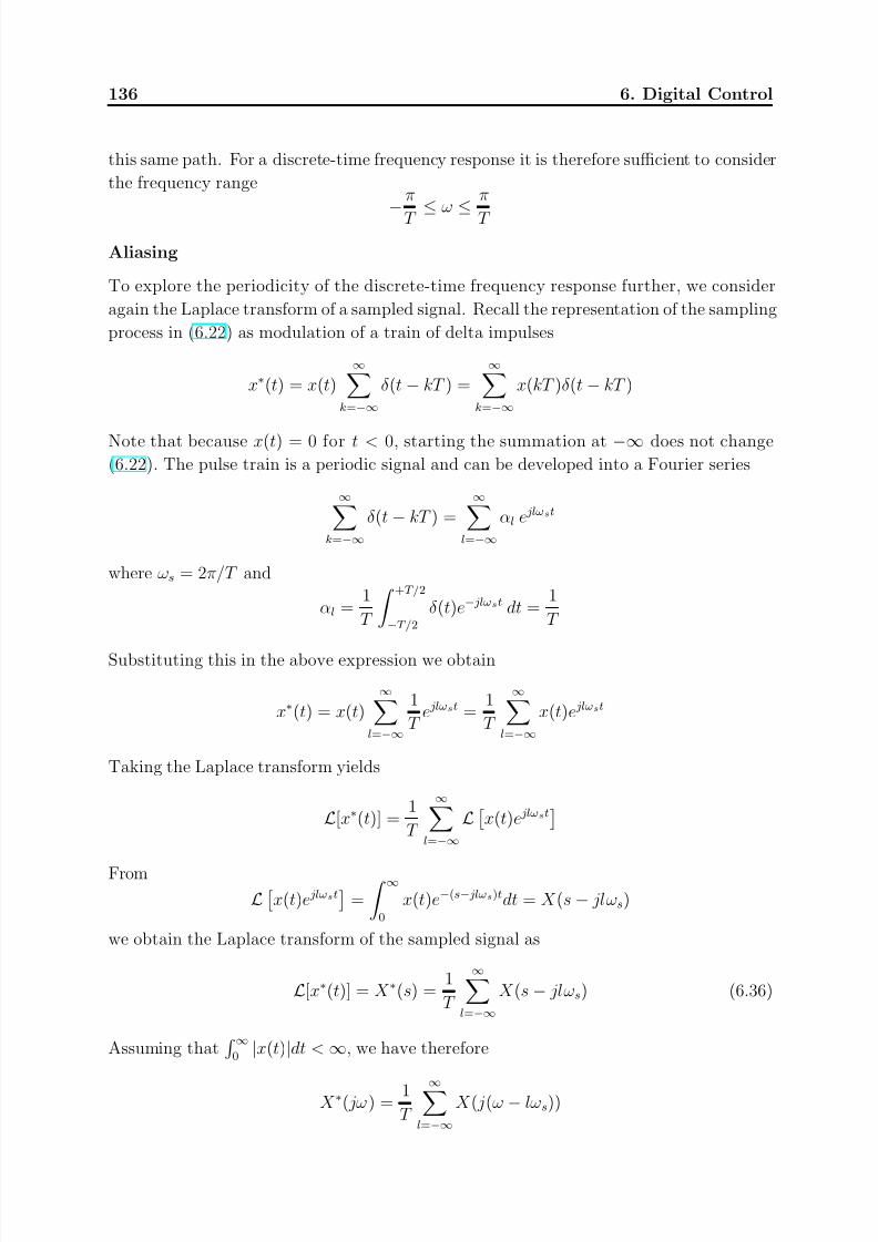
7/28/2019 Control System Theory and Design
http://slidepdf.com/reader/full/control-system-theory-and-design 144/290
136 6. Digital Control
this same path. For a discrete-time frequency response it is therefore sufficient to consider
the frequency range
−π
T ≤ω
≤π
T
Aliasing
To explore the periodicity of the discrete-time frequency response further, we consider
again the Laplace transform of a sampled signal. Recall the representation of the sampling
process in (6.22) as modulation of a train of delta impulses
x∗(t) = x(t)∞
k=−∞δ (t − kT ) =
∞k=−∞
x(kT )δ (t − kT )
Note that because x(t) = 0 for t < 0, starting the summation at −∞ does not change(6.22). The pulse train is a periodic signal and can be developed into a Fourier series
∞k=−∞
δ (t − kT ) =∞
l=−∞αl e jlωst
where ωs = 2π/T and
αl =1
T
+T /2
−T /2
δ (t)e− jlωst dt =1
T
Substituting this in the above expression we obtain
x∗(t) = x(t)∞
l=−∞
1
T e jlωst =
1
T
∞l=−∞
x(t)e jlωst
Taking the Laplace transform yields
L[x∗(t)] =1
T
∞l=−∞
L x(t)e jlωst
From
L x(t)e jlωst
=
∞0
x(t)e−(s− jlωs)tdt = X (s − jlωs)
we obtain the Laplace transform of the sampled signal as
L[x∗(t)] = X ∗(s) =1
T
∞l=−∞
X (s − jlωs) (6.36)
Assuming that
∞0
|x(t)|dt < ∞, we have therefore
X ∗( jω) = 1T
∞l=−∞
X ( j(ω − lωs))

7/28/2019 Control System Theory and Design
http://slidepdf.com/reader/full/control-system-theory-and-design 145/290
6.4. Frequency Response of Sampled-Data Systems 137
This is the superposition on the jω-axis of the transform of the original continuous-time
signal and its replications shifted by lωs, l = ±1, ±2, . . . If the signal x(t) contains no
frequency components at ω > ωb and if ωb < ωs
2, then the replicated spectra do not overlap,
and the original signal could theoretically be recovered by ideal low pass filtering. Fig.
6.12 illustrates this important result, which is in fact a statement of Shannon’s sampling
theorem : a signal x(t) can only be exactly reconstructed from its sampled version x∗(t)
if ωs > 2ωb, i.e. the sampling frequency is more than twice the signal bandwidth. The
maximum signal bandwidth
ωN =ωs
2=
π
T for which a reconstruction is possible, is called the Nyquist frequency . If the signal contains
frequency components above the Nyquist frequency, the sampling process will bring high
x(t)
0 ω−ωb ωb
|X ( jω)|
t
(a) Amplitude spectrum of continuous-time signal
x(t)
0−ωs ωs ω
|X ∗( jω)|
−ωb ωs
2
ωb−ωs
2t
(b) Amplitude spectrum of sampled signal, ωs > 2ωb
ωs ω
|X ∗( jω)|
t
x(t)
0 ωs
2−ωs
2
−ωs
(c) Amplitude spectrum of sampled signal, ωs < 2ωb
Figure 6.12: Aliasing effect of sampling

7/28/2019 Control System Theory and Design
http://slidepdf.com/reader/full/control-system-theory-and-design 146/290
138 6. Digital Control
frequency components back into the range below the Nyquist frequency and thus distort
the original signal. This effect is known as aliasing . A common measure called anti-
aliasing is to low-pass filter a signal before sampling with a filter bandwidth below the
Nyquist frequency but well above the signal bandwidth.
The frequency response of a sampled-data system including a zero-order hold is discussed
in Exercises 6.14 and 6.15.
Choice of Sampling Frequency
The sampling theorem suggests a lower bound on the sampling frequency for a digital con-
trol system: it must be higher than twice the bandwidth of the system, for otherwise the
information about the underlying continuous-time signals carried by the sampled signals
will be distorted. In practice, the sampling frequency is chosen higher than this. Whena digital controller is obtained via continuous-time design and Tustin approximation, the
time delay of T /2 resulting from the approximation demands a sampling frequency of at
least 20 ∼ 30ωb, as discussed earlier.
On the other hand, in the case of a direct discrete-time design with plant model (6.27), the
discretization is exact if a zero-order hold is present at plant input, even if sampling is slow.
However, it is important to realize that between sampling instants the control system is
effectively operating in open loop - the feedback loop is closed only in the sampling instants.
The effect of a disturbance occurring between two sampling instants will not be detected
and acted against before the following sampling instant. If the sampling time is long, the
effect of such a disturbance may be significant. A rule of thumb is to choose the sampling
rate at least five to ten times larger than the system bandwidth.

7/28/2019 Control System Theory and Design
http://slidepdf.com/reader/full/control-system-theory-and-design 147/290
Exercises 139
Exercises
Problem 6.1
a) For the discrete-time system with transfer function
G(z ) =2z 2 − 6z
2z 2 − 6z + 4
use polynomial division to determine the first 3 values of the impulse response of
the system.
b) By partial fraction expansion, determine the response of the system
G(z ) =1
1 − 2z −1
to the input
u(k) = 2e−kσ(k)
Problem 6.2
a) Show that∞
k=0
x(k)z −k −∞
k=0
x(k − 1)z −k = X (z ) − z −1X (z )
and, with x(k) = 0 when k < 0, that:
limz→1
∞k=0
[x(k)z −k − x(k − 1)z −k] = limk→∞
x(k)
b) Use the result from (a) to prove the Final Value Theorem for discrete-time signals
limk→∞
x(k) = limz→1
(z − 1)X (z )

7/28/2019 Control System Theory and Design
http://slidepdf.com/reader/full/control-system-theory-and-design 148/290
140 6. Digital Control
Problem 6.3
a) For a given sampling time T , sketch in the z -plane the regions corresponding to thefollowing regions in the s-plane: Re(s) and Im(s) refer to the real and imaginary
parts of a complex point s respectively.
i) Re(s) < −0.1T
, Re(s) < −0.5T
and Re(s) < −1.0T
ii) |Im(s)| < 0.5 πT
, |Im(s)| < 1.0 πT
and |Im(s)| < 1.5 πT
b) For a second order system, sketch lines in the z -plane corresponding to constant
damping ratios ζ = 0, 0.5 and 1.
c) For a second order system, sketch lines in the z -plane corresponding to constant
natural frequencies ωn = π2T
and πT
.
Problem 6.4
For the discrete-time system governed by the difference equation
y(k) + a1y(k − 1) + a2y(k − 2) + a3y(k − 3) = b1u(k − 1) + b2u(k − 2) + b3u(k − 3)
construct a state space model in controller canonical form, similar to the controller formfor continuous system. Sketch the corresponding block diagram.
Problem 6.5
Consider a plant with continuous transfer function
G(s) =b
s + a, a > 0
This plant is to be controlled by a controller K as shown in figure 6.13.
Gr y-
K
Figure 6.13: Closed-loop system
a) At first, G(s) is to be controlled using a continuous-time proportional feedback
controller K (s) = K p. Sketch the continuous-time root locus for a = 2 and b = 1.

7/28/2019 Control System Theory and Design
http://slidepdf.com/reader/full/control-system-theory-and-design 149/290
Exercises 141
b) Calculate an exact (zero-order-hold) discretization Gd(z ) of G(s) as a function of a
and b.
c) The plant is now to be controlled with the discrete-time proportional feedback con-troller K d(z ) = K pd and sampling time T = 0.2. Using the discrete-time plant
transfer function Gd(z ) from (b), sketch the discrete-time root locus with a = 2 and
b = 1. At what value of K pd does the system become unstable?
d) Using the continuous-time and discrete-time root loci, compare the closed-loop be-
haviour as K p → ∞ and K pd → ∞ for the system with continuous-time and discrete-
time controllers, respectively. Describe qualitatively why this behaviour occurs.
e) Create a Simulink model to compare the following closed-loop responses (a = 2,
b = 1)
i) with continuous-time plant and continuous-time controller where K p = 5
ii) with the continuous-time plant and discrete-time controller where K pd = 5
iii) with discretized plant from (b) and the discrete-time controller where K pd = 5.
Hint : Generate the discrete-time controller using the command c2d with the option
’tustin’.
Problem 6.6
Consider a continuous-time system with transfer function
G(s) =1
s2
This system is to be controlled as shown in Figure 6.13.
a) Calculate the exact (zero-order-hold) discretization Gd(z ) of G(s).
b) Sketch the root loci for the continuous-time plant and for the discrete-time plant,
each with proportional controllers. Can the plant be stabilized using either a
continuous-time or discrete-time proportional controller?
c) Gd(z ) is now to be controlled with a discrete-time PD-controller
K d(z ) = K pd(1 + T d(1 − z −1))
Show that this can be written as
K d
(z ) = K pd2
z − α
z
where α is a function of T d and K pd2 is K pd/(1 − α).

7/28/2019 Control System Theory and Design
http://slidepdf.com/reader/full/control-system-theory-and-design 150/290
142 6. Digital Control
d) Use rltool to find K pd2 and α so that a settling time < 2.0 and a damping ratio
ζ ≈ 0.7 are achieved. Use a sampling time T = 0.2 s.
Hint: You can use the design constraints settling time and damping ratio in rltool .
e) Use rltool again to calculate K p and α, so that the settling time < 4.5 and ζ ≈ 0.707.
This time use a sampling period of T = 0.5 s. Is it possible to achieve a settling
time < 2.0 with a discrete-time PD controller with T = 0.5 s?
Problem 6.7
a) Use Matlab to design a state feedback dead-beat controller K db for the discretized
double integrator Gd(z ) from Problem 6.6. You can either use the function ackerif available in your Matlab distribution, or place where you set the desired pole
locations to values close to 0 (place requires distinct pole locations, e.g. [0 1e-5]).
b) Use Matlab and Simulink to construct the closed loop system consisting of plant
G(s), the discrete state feedback controller K db, a sampler and a zero order hold
unit, and a disturbance at input of G(s). Plot the step response of the output of
G(s) to this disturbance.
Problem 6.8
This problem refers to the state space model of the turbogenerator and the continuous-
time controller and observer designed in Problem 5.15. You can use the script file
cs5_tgen_LQG.m to generate the controller..
a) Use Matlab to generate Tustin-approximation Ki of the controller with sampling
times T s = 0.02 and T s = 0.5.
Hint: You need to determine the Tustin approximation of the complete controller,
including the state feedback controller, Kalman filter and integrators. One (of many)ways to do this is to use the Matlab function linmod with a Simulink model of the
complete controller.
b) Simulate the response of the closed-loop system with both discretized controllers
(for T s = 0.02, 0.5) to a disturbance d1(t) = σ(t). Compare your response with the
one obtained in Problem 5.15.
c) Discretise the augmented plant (that is, including the integrators) for T s = 0.02 and
T s = 0.5. For each of these discretized systems design an LQG controller with the
same performance weights as in 5.15.
Hint: Use the command dlqr to design a discrete LQR controller and Kalman filter.

7/28/2019 Control System Theory and Design
http://slidepdf.com/reader/full/control-system-theory-and-design 151/290
Exercises 143
d) Compare the performance achieved with discrete time controllers of part a) and
c) for disturbance d1(t) = σ(t).
e) Simulate the response of the controller from exercise 5.15 and the disturbance d1 =σ(z ), but with a delay of 0.25 s between the controller output and the plant input.
Compare your answer with the response obtained in part b).
Hint: Use either Pad’e approximation, if you are performing the simulation in Mat-
lab, or transport delay block if you are using Simulink.
Problem 6.9
Consider a system with impulse response g(k) and transfer function
G(z ) =∞
k=0
g(k)z −k
Show that the response y(k) to an input signal u(k) with z-transform
U (z ) =∞
k=0
u(k)z −k
is given by
yk =k
l=0
g(l)u(k − l)
Problem 6.10
The discrete-time system G(z ) is described by the following set of matrices:
Φ = 0 0 1
0 0.2 2
0 0 0.1 , Γ = 0
1
1 , C = 2 1 0 , D = 0
a) Compute the impulse response of the system for the first 4 sampling instants.
b) Compute the system response to an input signal u = 5, 0, −1, 2. Consider zero
initial conditions.
Problem 6.11
The locations of zeros of a discrete-time system produced by exact (zero-order-hold)
discretization of a continuous-time system can be approximated by the model shown in
Figure 6.11.

7/28/2019 Control System Theory and Design
http://slidepdf.com/reader/full/control-system-theory-and-design 152/290
144 6. Digital Control
a) What zeros would you therefore expect, when the continuous-time systems
(i)
G(s) = s + 1s2 + 4s + 1
(ii)
G(s) =1
s3 + s2 + s
are sampled at high sampling rates with a zero order hold?
Hint: Calculate a state space model of the exact discretization of 1/sn−m
b) Check the results from (a) with the Matlab function c2d. For which sampling
times is the sampled system (ii) minimum phase? For which sampling times is itnon-minimum phase?
Problem 6.12
Practical representations of digital signals have finite word-length. Explain why this can
lead to problems if high sampling rates are used.
Hint: What happens to the locations of the poles and to the system matrix of a discrete-
time state space model if the sampling time approaches zero?
Problem 6.13
Consider the system
G(s) =0.2
s + 0.2
a) What is the time constant (τ ), bandwidth and gain of G(s).
b) Compute the frequency ω3 of a sinusoidal signal u(t) = sin(ω3t), which when appliedas an to G(s) it will generate an output y(t) with amplitude 3 dB smaller than the
steady-state gain.
c) The system is to be controlled in closed-loop as in Fig. 6.10. Assume that the
closed-loop bandwidth is the same as the bandwidth of the plant. What sampling
times T s are acceptable for the task?

7/28/2019 Control System Theory and Design
http://slidepdf.com/reader/full/control-system-theory-and-design 153/290
Exercises 145
Problem 6.14
Figure 6.14 shows a delta sampler with a zero-order hold (zoh ) unit.
u(t) zohT
y(t)
δ
u∗(t)
Figure 6.14: Zero order hold with delta sampler
a) Find an expression for y(t) as a function of u(t) at the sampling instants.
Hint: Use positive and negative step functions to represent the signal y(t).
b) Calculate the Laplace transform Y (s) of the output signal as a function of U (s).
c) Show that the transfer function of the zoh unit is
Gzoh(s) =Y (s)
U ∗(s)=
1
s(1 − e−T s)
d) Show using (c) that the frequency response of the zoh unit is
Gzoh( jω) = T sin(ωT /2)
ωT /2e−
12T jω
Sketch the bode diagram of the sample and hold unit for T = 1s.
Problem 6.15
The frequency response of the system in Figure 6.15 is to be investigated, where
G(s) =1
s + 1
u∗(t)
T G(s)zoh
δ
u(t) y(t)
Figure 6.15: Sampler and system G(s)

7/28/2019 Control System Theory and Design
http://slidepdf.com/reader/full/control-system-theory-and-design 154/290
146 6. Digital Control
a) Calculate u∗(t) when u(t) = sin ωt.
Hint: Represent the sequence of delta impulses associated with the delta-sampler by
a real Fourier series ∞
k=−∞δ (t − kT ) =
1
T
1 + 2
∞l=1
cos lωst
b) Simulate the response to the input signal in (a) for the frequencies ω = 2 rad/s,
ω = 20 rad/s and ω = 60 rad/s when the sampling period is T = 0.05 s. Interpret
the simulation with the help of the results in (a) and Problem 6.14.d. For the
simulation, use the Simulink model cs6_simzoh.mdl

7/28/2019 Control System Theory and Design
http://slidepdf.com/reader/full/control-system-theory-and-design 155/290
Chapter 7
System Identification
All methods for designing and analyzing control systems that have been introduced in
this course are model based , i.e. it is assumed that a dynamic plant model in the form
of a transfer function or state space realization is available. In practice, obtaining such
a model can take up a significant part of the time required for solving a given control
problem. In Exercises 1.1, 1.2 or 2.6, state space models of physical systems were derived
from the knowledge of the underlying physical laws. However, such physical modelling
can become difficult if the plant dynamics are complex and not well understood. An
alternative is to obtain a plant model experimentally by measuring the response of the
plant to suitable test signals; this approach is known as system identification . Becauseno physical insight into the plant behaviour is utilized, this method is also referred to as
black box modelling . This chapter gives an introduction to the basic concepts of system
identification.
Transfer functions and state space models are called parametric models , because the com-
plete information about the dynamic behaviour of the system is contained in a fixed
number of parameters - e.g. the coefficients of the transfer function polynomials or the
entries of the matrices of a state space model. Nonparametric models on the other hand
are representations of plant dynamics that cannot be expressed by a finite number of
parameters, such as the shape of the frequency response or the impulse response of thesystem. In this chapter we will consider the experimental identification of parametric
plant models. Because the input-output data used for system identification are usually
sampled-data sequences, the identified models are discrete-time models. After introducing
the concept of a linear regression model in Section 7.1, we will discuss the identification
of transfer function models for SISO systems in Section 7.2. Sections 7.3 and 7.4 then
present two recently developed techniques for identifying SISO and MIMO state space
models

7/28/2019 Control System Theory and Design
http://slidepdf.com/reader/full/control-system-theory-and-design 156/290
148 7. System Identification
7.1 Least Squares Estimation
Assume that we are observing a process - characterized by a quantity y(t) - at time in-stants t = 0, T, 2T , . . . where T is a given sampling time. Using the shorthand notation
introduced earlier and suppressing the sampling time, this observation yields a data se-
quence y(k), k = 0, 1, 2, . . . Assume further that the process variable y(k) at time instant
kT depends linearly on the values of other variables m1(k), m2(k), . . . , mn(k) which are
known and available at the same time. A linear process model is then
y(k) = m1(k) p1 + m2(k) p2 + . . . + mn(k) pn + e(k) (7.1)
where the dependence on the measured variables is determined by the parameters p1, p2, . . . , pn.
The term
e(k) = y(k) − m1(k) p1 − m2(k) p2 − . . . − mn(k) pn
is added to allow for modelling errors, e.g. measurement errors or inaccurate knowledge
of values of the parameters pi. Further modelling errors could arise if the true process
depends on the measured variables in a nonlinear way, or if it depends on additional
variables that are not included in the above model.
The model (7.1) can be written in a more compact form as a linear regression model
y(k) = [m1(k) . . . mn(k)] p1
..
. pn
+ e(k) = m
T
(k) p + e(k) (7.2)
where two column vectors - the vector of regression variables m(k) and the parameter
vector p - have been introduced. Given a set of measured data y(l) and m(l), l =
0, 1, . . . , k, we can now pose the least squares estimation problem : find the parameter
vector p that best fits the data, in the sense that the sum of the squared errors
V ( p) =k
l=0
e2(l) (7.3)
is minimized.
Example 7.1
Suppose a transfer function model of an unknown system is to be identified which is
thought to be governed by a first order linear difference equation. The task is then to
find parameters a and b of the transfer function
G(z ) =bz −1
1 + az −1
that lead to a good fit between measured data and output data predicted by the transfer
function model. The situation is illustrated in Fig. 7.1: the same input sequence u(k)

7/28/2019 Control System Theory and Design
http://slidepdf.com/reader/full/control-system-theory-and-design 157/290
7.1. Least Squares Estimation 149
is applied to the unknown system and to the model G(z ), yielding the actual system
response y(k) and the response y(k) predicted by the model, respectively. The modelling
error is
e(k) = y(k) − y(k)
This problem can be expressed in the form of a linear regression model by writing the
difference equation of the system as
y(k) = −ay(k − 1) + bu(k − 1) + e(k)
= [−y(k − 1) u(k − 1)]
a
b
+ e(k)
= mT (k) p + e(k) = y(k) + e(k)
ykSystem
G(z )
uk ek-
yk
Figure 7.1: Identification of a transfer function model
Solving the Least Squares Estimation Problem
If a data set y(l), u(l), l = 0, 1, 2, . . . , k is available, we can arrange it in the form
Y = Mp + E (7.4)
where we define
Y =
y(0)...
y(k)
, M =
mT (0)...
mT (k)
, E =
e(0)...
e(k)
Similarly, we introduce the vector
Y = Mp
of predicted outputs. Assuming initially that the unknown system can indeed be accu-
rately described by a linear model of the assumed order, and that there are no measure-
ment errors, the modelling error will be zero if the parameter vector p takes its “true”
value: in that case we have Y = Y , or
M p = Y (7.5)
If we have more measurements available than model parameters, i.e. if k > n, this is an
overdetermined system of equations. Multiplying from left by M T
yields
M T M p = M T Y (7.6)

7/28/2019 Control System Theory and Design
http://slidepdf.com/reader/full/control-system-theory-and-design 158/290
150 7. System Identification
This equation is called the normal equation associated with the given estimation problem.
If M has full column rank, the matrix M T M ∈ IRn×n is non-singular, and we can compute
p = (M T M )−1M T Y (7.7)
However, the parameter vector p obtained from (7.7) will satisfy (7.5) only if the system
is indeed exactly governed by a linear difference equation of the assumed order, and if
there are no measurement errors. In real life problems, neither condition will be met, so
that p will not satisfy (7.5) but only (7.4) with E = 0. The best we can then achieve is
to find the parameter vector p that is associated with the “smallest modelling error” -
in other words the closest approximation we can get with this model in the presence of
measurement errors. The following result is derived in Exercise 7.1.
Theorem 7.1
The sum of square errors V ( p) (7.3) is minimized if the parameter vector satisfies the
normal equation (7.6).
If the matrix M T M is nonsingular, the minimizing parameter vector is given by (7.7).
Geometric Interpretation
A geometric interpretation of the normal equation goes as follows. Rewrite (7.4) as
E = Y − Mp
or e(0)
...
e(k)
=
y(0)
...
y(k)
−
m1(0)
...
m1(k)
p1 − . . . −
mn(0)
...
mn(k)
pn
Introducing the column vectors
ϕi =
mi(0)...
mi(k)
, i = 1, . . . , n
we thus have
E = Y − ϕ1 p1 − . . . − ϕn pn
If the true system can be accurately described by the assumed linear model and if there are
no measurement errors, then Y would be in the space spanned by the vectors ϕ1 . . . ϕn.
In real life, unmodelled features of the system and measurement errors will in general
lead to a vector Y that is outside the data space. The estimation problem can then be
interpreted as searching for the linear combination of the vectors ϕ1 . . . ϕn that comes

7/28/2019 Control System Theory and Design
http://slidepdf.com/reader/full/control-system-theory-and-design 159/290
7.2. Estimation of Transfer Function Models 151
ϕ2
p2
p1
ϕ1
Y
E
Y
Figure 7.2: Geometric interpretation of the least squares estimation problem
closest to the vector Y , i.e. that minimizes the squared error E T E . This is illustrated in
Fig. 7.2 for the special case n = 2: what we are looking for is the projection Y of the
vector Y onto the space (a plane if n = 2) spanned by the measurement vectors ϕi, and
Y is the vector closest to Y if the error E is orthogonal to this space (plane). But E is
orthogonal to this space if it is orthogonal to each of the measurement vectors, i.e. if it
satisfies
ϕT i E = 0, i = 1, . . . , n
This can be written in a more compact form as M T E = 0 or
M T (Y − M p) = 0
which is just the normal equation (7.6).
7.2 Estimation of Transfer Function Models
We will now apply the idea of least squares estimation to identify a transfer function model
of a system from measured input and output data. Thus, assume that data sequences
u(0), . . . , u(k) and y(0), . . . , y(k) are available and that we want to find the pulse
transfer function that gives the best fit between input and output data. In order to apply
the above estimation technique, we need to fix the number of parameters, in this case the
order of numerator and denominator polynomial of the estimated transfer function. We
will initially assume for simplicity that the system to be identified can be modelled by
the difference equation
y(k) = b1u(k − 1) + b2u(k − 2) + . . . + bnu(k − n) (7.8)
which means there is no autoregressive component in the output (the ais are zero) - we
will later remove this assumption. The difference equation can be written in regressor

7/28/2019 Control System Theory and Design
http://slidepdf.com/reader/full/control-system-theory-and-design 160/290
152 7. System Identification
form as
y(k) = [u(k
−1) u(k
−2) . . . u(k
−n)]
b1...
bn = mT (k) p
The measurement matrix M takes the form
M =
u(n − 1) u(n − 2) . . . u(0)
u(n) u(n − 1) . . . u(1)...
...
u(k) u(k − 1) . . . u(k − n + 1)
where we take mT (n) as the first row, and we have
M T M =
ki=n−1 u2
i
ki=n−1 uiui−1 . . .
ki=n−1 uiui−n+1k
i=n−1 ui−1ui
ki=n−1 u2
i−1 . . .k
i=n−1 ui−1ui−n+1
.... . .
...ki=n−1 ui−n+1ui
ki=n−1 ui−n+1ui−1 . . .
ki=n−1 u2
i−n+1
where we used the shorthand notation ui for u(i). For a solution (7.7) to the estimation
problem to exist, this n
×n matrix needs to be invertible. This requirement places a
condition on the input sequence u(0), . . . , u(k). For example, it is obvious that with
a constant input sequence 1, . . . , 1 the rank of M T M will be one and a solution for a
model with more than one estimated parameter will in general not exist. To explore this
further, we will use the empirical autocorrelation of the data sequence u(k), defined as
cuu(l) = limk→∞
1
k
ki=1
u(i)u(i − l)
Introducing the matrix
C uu(n) =
cuu(0) cuu(1) . . . cuu(n − 1)cuu(1) cuu(0) . . . cuu(n − 2)
.... . .
...
cuu(n − 1) cuu(n − 2) . . . cuu(0)
we find that
limk→∞
1
kM T M = C uu(n)
Thus, for sufficiently long data sequences (when the end effects can be neglected and we
can consider all sums as taken from 1 to k) we may interpret the matrix M T M as a scaled
version of the empirical covariance C uu(n) of the input signal.

7/28/2019 Control System Theory and Design
http://slidepdf.com/reader/full/control-system-theory-and-design 161/290
7.2. Estimation of Transfer Function Models 153
Persistent Excitation
The condition that the matrix M T M must have full rank is called an excitation condition
- the input signal must be sufficiently rich to excite all dynamic modes of the system.We have seen that for long data sequences we can consider the matrix C uu(n) instead of
M T M . The following definition provides a measure for the richness of an input signal.
Definition 7.1
A signal u(k) is said to be persistently exciting of order n if the matrix C uu(n) is positive
definite.
The next result is useful for checking whether a signal is persistently exciting of a given
order.
Theorem 7.2
A signal u(k) is persistently exciting of order n if and only if
limk→∞
1
k
kl=0
a(z )u(l)
2> 0 ∀a(z ) : deg a(z ) ≤ n (7.9)
Here a(z ) is a polynomial in the forward shift operator z , i.e.
a(z ) = a0 + a1z + a2z 2 + . . . + an−1z n−1
Recall that the forward shift operator is defined by
zu(l) = u(l + 1)
With these definitions, multiplying a signal u(k) by a(z ) yields
a(z )u(l) = a0u(l) + a1u(l + 1) + a2u(l + 2) + . . . + an−1u(l + n − 1)
It is straightforward to prove the above Theorem by observing that the sum on the left
hand side of the inequality can be rewritten as
limk→∞
1
k
kl=0
(a(z )u(l))2 = aT C uu(n)a
where aT = [an−1 an−2 . . . a0]
Theorem 7.2 can be used to determine an upper bound on the order of the persistent
excitation of a given signal: if one can find a polynomial a(z ) of order n that does not
satisfy (7.9), then the signal is not persistently exciting (PE) of order n. This idea can
be used to show that

7/28/2019 Control System Theory and Design
http://slidepdf.com/reader/full/control-system-theory-and-design 162/290
154 7. System Identification
• an impulse δ (k) is PE of order 0
• a step function σ(k) is PE of order 1
• a sine wave is PE of order 2
• white noise is PE of any order
For step functions and white noise, this is discussed in Exercise 7.2. White noise is there-
fore commonly used as test input when a linear model is to be identified experimentally.
ARX Models
The model (7.8) was based on the assumption that the present output does not depend
on past outputs, i.e. there is no autoregressive component in the output. We now remove
this assumption and consider the model
y(k) = −a1y(k − 1) − . . . − any(k − n) + b1u(k − 1) + . . . bnu(k − n)
= [−y(k − 1) . . . − y(k − n) u(k − 1) . . . u(k − n)]
a1...
an
b1...
bn
which corresponds to the difference equation model introduced for discrete-time systems
in the previous chapter. Such a model is called an ARX model , where ARX stands
for AutoRegressive with eXogenous input. The results discussed in this section can be
extended to ARX models by using the empirical cross-covariance function
cuy(l) = limk→∞
1
k
ki=1
u(i)y(i − l)
It follows then that
limk→∞
1
kM T M =
C yy −C uy
−C uy C uu
where the matrices C yy and C uy are defined in the same way as C uu.
The least-squares estimation of an ARX model from measured data is illustrated in Ex-
ercise 7.4.

7/28/2019 Control System Theory and Design
http://slidepdf.com/reader/full/control-system-theory-and-design 163/290
7.3. Subspace Identification of State Space Models 155
7.3 Subspace Identification of State Space Models
The discussion in the previous section was limited to SISO transfer function models.The approach presented there can be extended to cover MIMO models in ARX form, but
working with multivariable systems is usually more convenient in a state space framework.
In this and the following section we present a recently developed approach to estimating
SISO and MIMO state space models.
To introduce the idea, we begin with a SISO state space model
x(k + 1) = Φx(k) + Γu(k), x(0) = 0
y(k) = cx(k) + du(k)
Note that we use the same symbol Γ for discrete-time SISO and MIMO models, in a SISO
model it represents a column vector. Now assume that x(0) = 0, and consider the impulse
response of the above model, i.e. the response to the input u(k) = δ (k). Observing that
for k > 0 we have x(k) = Φk−1Γ, we find that the impulse response g(k) is given by
g(k) =
0, k < 0
d, k = 0
cΦk−1Γ, k > 0
The values d, cΓ, cΦΓ, . . . of the impulse response sequence are called the Markov parameters of the system.
Turning now to multivariable systems, we first need to clarify what we mean by the
impulse response of a MIMO model
x(k + 1) = Φx(k) + Γu(k), x(0) = 0
y(k) = Cx(k) + Du(k) (7.10)
We can apply a unit impulse to one input channel at a time and observe the resulting
response at each output channel
uδi(k) =
0...
0
δ (k)
0...
0
→ yδi(k) =
g1i(k)
...
gli(k)
Here δ (k) is placed in the ith entry of the input vector, while all other inputs are zero.
An entry g ji(k) in the output vector represents the response at output channel j to a unit

7/28/2019 Control System Theory and Design
http://slidepdf.com/reader/full/control-system-theory-and-design 164/290
156 7. System Identification
impulse applied at input channel i. The complete information about the impulse responses
from each input to each output can then be represented by the impulse response matrix
g(k) =
g11(k) . . . g1m(k)...
...
gl1(k) . . . glm(k)
Introducing the notation
Γ = [Γ1 Γ2 . . . Γm], D = [d1 d2 . . . dm]
where Γi and di denote the ith column of the matrices Γ and D, respectively, we find that
with input uδi(k) we have xδi(k) = Φk−1Γi for k > 0, and at k = 0 we have yδi(k) = di.
Combining the responses to impulses at all input channels, we obtain
g(k) = [yδ1(k) . . . yδm(k)] =
0, k < 0
D, k = 0
C Φk−1Γ, k > 0
(7.11)
The impulse response describes input-output properties of a system, and we would expect
it to be independent of a particular coordinate basis that has been chosen for a given
state space model. This seems to contradict the fact that the impulse response in (7.11)
is given in terms of the matrices (Φ, Γ, C ) of a state space model, which clearly depend
on the choice of coordinate basis. However, it is easily checked that applying a similarity
transformation T - which yields a realization (T −1ΦT, T −1Γ, CT ) - will not change theimpulse response.
Constructing a Model from the Impulse Response
Assume that measured impulse response data of a system are available and have been
arranged in the form of a matrix
H k =
g(1) g(2) g(3) . . . g(k)
g(2) g(3) . . . g(k + 1)
g(3)...
......
g(k) g(k + 1) . . . g(2k − 1)
A matrix with this structure is called a Hankel matrix if the g(l) are scalar, and a block-
Hankel matrix if the g(l) are matrices. Using (7.11) in the above we obtain
H k =
C Γ C ΦΓ C Φ2Γ . . . C Φk−1Γ
C ΦΓ C Φ2Γ . . . C ΦkΓ
C Φ2Γ...
... ...
C Φk−1Γ C ΦkΓ . . . C Φ2k−2Γ
(7.12)

7/28/2019 Control System Theory and Design
http://slidepdf.com/reader/full/control-system-theory-and-design 165/290
7.3. Subspace Identification of State Space Models 157
Assume the number of samples is sufficiently large so that k > n, where n is the order
of the state space model. Note that at this point we know nothing about the system
apart from its impulse response. In particular, we do not know the order n of the system.
Important in this context is the rank of the matrix H k. To investigate this, we first observe
that we can factor H k as
H k =
C
C Φ...
C Φk−1
[Γ ΦΓ . . . Φk−1Γ] = OkCk
Here Ok and Ck are the extended observability and controllability matrices , respectively,
of the model (7.10), where the term “extended” is added because the number of samples
k is greater than the expected order n of the system. Assuming that we are interested in
estimating a model (7.10) that represents a minimal realization of a system, i.e. if (Φ, Γ)
is controllable and (C, Φ) is observable, then we have
rank Ok = rank Ck = n
which implies
rank H k = n (7.13)
Thus, we can obtain the order from the measured data by computing the rank of H k.
The Ideal Case
Assume that for a given system with m inputs and l outputs the measured discrete-time
impulse response g(k) is available, and that we want to identify a discrete-time state
space model (Φ, Γ, C ). For systems where D = 0, the feedthrough matrix is given by
g(0). Initially we do not know the dynamic order of this model, but we assume that we
have a sufficient number of samples of the impulse response, so that we can form the
mk × lk matrix H k for a value of k that is larger than the expected order of the model. If
the impulse response data were indeed generated by a linear state space model of the form
(7.10) with n state variables, and if no measurement errors are present in the data, thenthe order n of the model can be easily determined by checking the rank of H k. Knowing
n we can then factor H k as
H k = M L, M ∈ IRlk×n, L ∈ IRn×mk
such that
rank M = rank L = n
This can be done using singular value decomposition as explained below. Note that this
factorization is not unique. Finally, we define the matrices M and L to be the extended
observability and controllability matrices
Ok = M, Ck = L

7/28/2019 Control System Theory and Design
http://slidepdf.com/reader/full/control-system-theory-and-design 166/290
158 7. System Identification
The first l rows of M therefore represent the measurement matrix C , and the first m
columns of L form the input matrix Γ. To find the state matrix Φ, define
Ok =
C Φ
...
C Φk
= OkΦ
Note that we can generate Ok from measured data by factorizing the larger Hankel matrix
H k+1 and removing the first l rows from Ok+1. Multiplying the above from the left by
OT k we obtain
OT k
OkΦ =
OT k
¯
Ok
Since Ok has full row rank, we can compute Φ from
Φ = (OT k Ok)−1OT
k Ok
The above describes a procedure for constructing the matrices Φ, Γ and C from measured
impulse response data. At this point a question arises: we know that a state space model
of a given system is not unique but depends on the coordinate basis chosen for the state
space. One could therefore ask where this choice was made in the above construction.
The answer is that the factorization H k = ML is not unique, in fact if M and L arefactors of rank n and if T is an arbitrary nonsingular n × n matrix, then it is easy to see
that MT and T −1L are also rank n factors of H k. With this latter choice we obtain
Ok = OkT, Ck = T −1Ck
From Chapters 2 and 3 we know however that these are the observability and controllabil-
ity matrices, respectively, of the model obtained by applying the similarity transformation
T to (Φ, Γ, C ). This shows that a choice of coordinate basis is made implicitly when H k
is factored into M L.
Modelling Errors and Measurement Noise
The above procedure for identifying a state space model relies on the assumption that
the measured data were indeed generated by a linear system and are not corrupted by
measurement noise. In practice, neither assumption will be true. One consequence of
this is that no matter how large k is chosen, the matrix H k will usually have full rank.
To extract information about the model order in spite of data being corrupted, one can
use the technique of singular value decomposition , a brief review of which is given in the
Appendix.

7/28/2019 Control System Theory and Design
http://slidepdf.com/reader/full/control-system-theory-and-design 167/290
7.3. Subspace Identification of State Space Models 159
Singular Value Decomposition
Consider a singular value decomposition of the data matrix H k ∈ IRkl×km
H k = QΣV T (7.14)
where Σ is a diagonal matrix with nonnegative diagonal entries, and Q and V are orthog-
onal, i.e. they satisfy
QQT = I kl, V V T = I km
Assume that the singular values are arranged in decreasing order such that
σ1 ≥ σ2 ≥ . . . ≥ σr > σr+1 = . . . σ p = 0
where p = min(kl,km). In this case we have rank H k = r, because an important fact
about singular value decomposition is that the rank of a matrix is equal to the numberof its nonzero singular values. Here σr+1 and all the following singular values are zero.
On the other hand, if the singular values σr+1, . . . , σ p are very small - much smaller than
σr - but nonzero, the matrix H k has full rank but is “close to being singular”. This
is precisely the situation we encounter when a block-Hankel matrix is constructed from
impulse response data that are corrupted by measurement noise. One of the powerful
features of the singular value decomposition is that it allows us to distinguish significant
information from noise effects by inspection of the singular values. An example is shown in
Fig. 7.3, where the singular values of a matrix are shown in decreasing order. If these were
the singular values of a Hankel matrix constructed from a measured impulse response, we
would conclude that the system dynamics can be described reasonably well by a 4 th order
model and that the remaining nonzero but small singular values represent noise effects.
σi
21 3 4 5 6 i
Figure 7.3: Determining the numerical rank
If σr+1 is much smaller than σr, we say that the numerical rank of H k is r. Another way
of looking at this is to write (7.14) as
H k = q 1 q 2 . . . q klσ1 0 0 . . . 0
.. . 0 . . . 0
0 σ p 0 . . . 0
vT 1
vT 2
...
vT km

7/28/2019 Control System Theory and Design
http://slidepdf.com/reader/full/control-system-theory-and-design 168/290
160 7. System Identification
where q i and vi represent the ith column of Q and V , respectively. Expanding the right
hand side column by column, we obtain
H k =
pi=1
σiq ivT i =
ri=1
σiq ivT i +
pi=r+1
σiq ivT i = QsΣsV T
s + QnΣnV T n
where Qs ∈ IRkl×r and V s ∈ IRkm×r are the matrices formed by the first r columns of Q
and V , respectively. The matrices Qn ∈ IRkl×(kl−r) and V n ∈ IRkm×(km−r) are similarly
formed by the remaining columns. If the singular values σr+1, . . . , σ p are much smaller
than σr, the last term on the right hand side can be neglected and we have
H k ≈ QsΣsV T s
or
H k ≈q 1 q 2 . . . q r
σ1 0 0 . . . 0
. . . 0 . . . 0
0 σr 0 . . . 0
vT 1
vT 2...
vT r
= QsΣ1/2s Σ1/2
s V T s
where r is the numerical rank of H k. Now taking r as the estimated model order n, we can
define the extended observability and controllability matrices Or ∈ IRkl×r and Cr ∈ IRkm×r
as
Or = QsΣ1/2s , Cr = Σ1/2
s V T s
A state space model (Φ, Γ, C ) of order n can then be obtained as in the case of ideal
measurements.
The identification of a state space model from the impulse response is illustrated in Ex-
ercise 7.5.
7.4 Direct Subspace Identification
The method outlined in the previous section assumes that the measured impulse response
is available. In practice it is usually better to use more general data, obtained for exampleby applying a white noise input signal. We will now present a technique for identifying
state space models without using the measured impulse response, referred to as direct
subspace identification .
Consider again the model (7.10). Beginning at time k, the output at successive time
instants is given by
y(k) = Cx(k) + Du(k)
y(k + 1) = C Φx(k) + C Γu(k) + Du(k + 1)
y(k + 2) = C Φ2x(k) + C ΦΓu(k) + C Γu(k + 1) + Du(k + 2)
...

7/28/2019 Control System Theory and Design
http://slidepdf.com/reader/full/control-system-theory-and-design 169/290
7.4. Direct Subspace Identification 161
Introducing the vectors
Y k =
y(k)
y(k + 1)...
y(k + α − 1)
, U k =
u(k)
u(k + 1)...
u(k + α − 1)
of input and output data, we can write
Y k = Oαx(k) + ΨαU k (7.15)
where
Oα =
C
C Φ
C Φ2
...
C Φα−1
, Ψα =
D 0 0 . . . 0
C Γ D 0 . . . 0
C ΦΓ C Γ D 0...
. . .. . .
C Φα−2Γ C Φα−1Γ . . . C Γ D
Assume that a sufficient number of measurements has been collected so that we can form
the input and output data matrices
Y = [Y 1 Y 2 . . . Y N ], U = [U 1 U 2 . . . U N ],
Define also the matrix of state variables
X = [x(1) x(2) . . . x(N )]
From (7.15), these data matrices satisfy
Y = OαX + Ψα U (7.16)
In this equation only U and Y are known; note that U ∈ IRmα×N . We assume that the
number (N + α − 1) of measurements - which is required to fill the above matrices - is
large enough such that α can be chosen greater than the expected model order, and N
such that N > mα. To identify a state space model, we need to estimate the matrices
Oα (from which C and Φ can be extracted) and Ψα (from which we get D and Γ).
Estimating the Term OαX
As a first step, we will eliminate the effect of the input data on the output data in (7.16)
and estimate the product OαX . This can be achieved by projecting the output data onto
the nullspace of the input data matrix U . The nullspace N ( U ) is defined as the space of
all vectors q that are made zero when multiplied from the left by U : N ( U ) = q : U q = 0
Now define the matrix Π as
Π = I − U T ( UU T )−1 U

7/28/2019 Control System Theory and Design
http://slidepdf.com/reader/full/control-system-theory-and-design 170/290
162 7. System Identification
All columns of Π are orthogonal to U , this can be seen from
U Π =
U − UU T (
UU T )−1
U = 0
Note that Π is constructed from measured data only. Here we assumed that ( UU T ) is
invertible, a condition for this is that the input is persistently exciting of order mα.
Multiplying equation (7.16) from the right by Π then yields
Y Π = (OαX + Ψα U )Π = OαX Π
The left hand side is known (because it is constructed from measured data), thus the
product OαX Π is known. Observing that Oα ∈ IRlα×n and X Π ∈ IRn×N , we can obtain
an estimate of the extended observability matrix by determining the numerical rank n
of the matrix Y Π and by factoring it into a left factor with n columns and full columnrank, and a right factor with n rows. This can be done by computing the singular value
decomposition
Y Π = QsΣsV T s + QnΣnV T
n ≈ QsΣ1/2s Σ1/2
s V T s
and by taking
Oα = QsΣ1/2s
Here again the order of the system is estimated by inspection of the singular values - this
time of the data matrix Y Π. From Oα the matrices C and Φ can be obtained as described
in the previous section.
Estimating the Term Ψα U We can now use the estimate of Oα to eliminate the first term on the right hand side of
(7.16). For this purpose, observe that from
QQT =
QT
s
QT n
[Qs Qn] =
I 0
0 I
we have QT n Qs = 0 and therefore QT
n
Oα
≈0. Thus, from (7.16) we obtain
QT nYU −R = QT
n Ψα
where U −R = U T ( UU T )−1 denotes the right inverse of U . The left hand side of this
equation and Qn are known, so that Ψα is the only unknown term. The matrices Γ and
D can then be obtained by solving a linear system of equations, details are omitted.

7/28/2019 Control System Theory and Design
http://slidepdf.com/reader/full/control-system-theory-and-design 171/290
Exercises 163
Exercises
Problem 7.1
Consider the sum of squared errors
V ( p) =k
l=0
e2(l) = E T E = (Y − Mp)T (Y − Mp)
introduced in (7.3). Show that V ( p) is minimized by the parameter vector p = ˆ p where
ˆ p = (M T M )−1M T Y
Hint: One way of proving the above is by the approach of completion of squares
Problem 7.2
a) Show that for the step function σ(k)
(z − 1)σ(k) = 1 at k = −1
and
(z − 1)σ(k) = 0 at k ≥ 0
b) If for a given signal u(k) there is at least one polynomial a(z ) of order n such that
limk→∞
1
k
kl=0
(a(z )u(l))2 = 0
what does this indicate about the order of persistent excitation u(k)?
c) Use the polynomial
a(z ) = z − 1
and the results from (a) and (b) to find the greatest possible order of persistent
excitation of a step function.
d) Calculate the empirical covariance matrix C uu(1) for the step function. Use this
matrix to show that the order of persistent excitation of a step function is 1.
e) Use the empirical covariance matrices C uu(1), C uu(2) . . . C uu(n) to show that the
order of persistent excitation of sampled white noise is arbitrarily high. Use the fact
that the correlation between white noise at times T and kT + T is 0.

7/28/2019 Control System Theory and Design
http://slidepdf.com/reader/full/control-system-theory-and-design 172/290
164 7. System Identification
Problem 7.3
a) For the input signal
u(k) = sin ωkT
show that
(z 2 − 2z cos ωT + 1)u(k) = 0
where T is the sampling time.
Hint: Determine (z 2−2z cos ωT +1)u(k) and simplify using trigonometric identities.
b) Find the greatest possible order of persistent excitation of the signal u(k)?
c) The autocorrelation function for any signal x(t) is defined as,
Rx(τ ) = limN →∞
1
N
N k=0
x(kT )x(kT ± τ )
It can be shown that for u(t) = sin ωt,
Ru(τ ) =1
2
cos ωτ
Using these facts show that for the signal u(k)
C uu(2) =1
2
1 cos ωT
cos ωT 1
Hint: Write the elements of C uu(2) in terms of the autocorrelation function.
c) What is the order of persistent excitation of the signal u(k) when
i) T = 2πω
ii) T = 2πω
Explain these results.

7/28/2019 Control System Theory and Design
http://slidepdf.com/reader/full/control-system-theory-and-design 173/290
Exercises 165
Problem 7.4
Download cs7_LSsysdat.mat. The MAT file contains sampled input and output signals
of a SISO system, where the input signal is a step (input u1, output y1), a sinusoid (input
u2, output y2) or white noise (input u3, output y3). A pulse transfer function is to be
determined that approximates the behaviour of the system from which the measurements
were taken.
a) From N samples of the inputs and N samples of the output create the measurement
matrix M for a system of order n. What is the dimension of the matrix M produced
from these data?
b) Determine the rank of the matrix M T M for
i) the sinusoid
ii) the white noise signal
Explain the results.
c) From output data generated from white noise, calculate a least squares estimate of
the model parameters.
d) i) Estimate the models of order 2, 3 and 4 using the white noise input signal.
ii) Validate the model for the step and sinusoidal input signals.
iii) What is the order of the system?
e) Explain the results from (d) with the help of Problems 7.2 and 7.3.b.
Problem 7.5
Download the Matlab script cs7_mkdata.m. This script generates the impulse responses
g(k) and gn(k) of a system with 2 inputs and 2 outputs. The sequence g(k) is noise free,
whereas gn(k) is corrupted by measurement noise.
a) Generate from the sequence g(k) the block Hankel matrix of the impulse response.
Estimate upper and lower limits for the order n of the system and determine by
factorization of the block Hankel matrix linear state space models of the system for
different values of the order n. Compare the impulse responses of the estimated
models with the output sequence g(k).
Hint: You can use the function mkhankel.m to generate the Hankel matrix.
b) Repeat the estimation for the noisy impulse response gn(k).

7/28/2019 Control System Theory and Design
http://slidepdf.com/reader/full/control-system-theory-and-design 174/290
166 7. System Identification
Problem 7.6
This exercise uses the Matlab Identification toolbox GUI ident to identify a state space
model from sets of data with two inputs and two outputs. The data is in the file
cs9_identGUI.mat.
Two sets data are contained in the file,iodata1 and iodata2. They are in the Matlab
format iddata that can be directly imported into ident.
a) Import the data set iodata1 and generate direct subspace identified models of
different orders using the command n4sid.
b) validate the models generated against the data set iodata2. What is the model
order that most effectively describes the plant behaviour?

7/28/2019 Control System Theory and Design
http://slidepdf.com/reader/full/control-system-theory-and-design 175/290
Chapter 8
Model Order Reduction
Modern state space design techniques - like those discussed in this course - produce
controllers of the same dynamic order as the generalized plant. Thus, when the system
to be controlled has a high dynamic order, the controller may be too complex to be
acceptable for implementation. In such cases, the plant model should be approximated
by a simplified model. Alternatively, a high-order controller can be approximated by a
low-order controller. This chapter gives a brief introduction to the topic of model order
reduction.
Consider a stable system with transfer function G(s) and state space realization
x = Ax + Bu, y = Cx + Du
with n dimensional state vector x. If the number of states n is very large, one could try
to find a model of lower order that behaves ”similar” to the original system. For example,
if some of the state variables do not have much effect on the system behaviour, one might
consider removing these states from the model. Thus, we need to know which states are
”important” for the model and which ones are not. The controllability Gramian and the
observability Gramian turn out to be helpful for answering this question.
Controllability Gramian
Recall the definition of the controllability Gramian
W c =
∞0
eAtBB T eAT t dt
A useful geometrical interpretation of W c - given here without proof - is the following.
Define the set S c as the set of all points in state space to which the state vector x(t) of the
system can be driven from the origin with an input signal u(τ ), 0 ≤ τ ≤ t, that satisfies t
0
uT (τ )u(τ )dτ ≤ 1

7/28/2019 Control System Theory and Design
http://slidepdf.com/reader/full/control-system-theory-and-design 176/290
168 8. Model Order Reduction
In other words: we consider all input signals with energy less than or equal to 1 (assume
that u(τ ) = 0 for τ > t). Compute the singular value decomposition of the controllability
Gramian
W c = V ΣV T
where
Σ = diag (σ1, σ2, . . . σn) and V = [v1 v2 . . . vn]
The singular values are ordered such that σ1 ≥ σ2 ≥ . . . ≥ σn as usual. The set S c of
points in the state space reachable with input energy 1 is then a hyper-ellipsoid centered
at the origin, with semi-axes in the directions of the columns vi of V , and length given by
the square root of the corresponding singular value. This is illustrated in Figure 8.1 for a
second order system. Note that v1 is the direction that is most easily controlled, whereas
small singular values indicate directions which are difficult to control.
σ
1/2
2 v2
σ1/21 v1
S c
x1
x2
Figure 8.1: Interpretation of the controllability Gramian
Observability Gramian
A similar interpretation can be given for the observability Gramian
W o =
∞0
eAT tC T CeAt dt
Define the set S o as the set of all points in the state space which - when taken as initial
conditions x(0) - lead to a zero-input response y(t) that satisfies ∞0
yT (t)y(t)dt ≤ 1
Again the singular value decomposition
W o = V ΣV T

7/28/2019 Control System Theory and Design
http://slidepdf.com/reader/full/control-system-theory-and-design 177/290
169
where
Σ = diag (σ1, σ2, . . . σn) and V = [v1 v2 . . . vn]
determines the set S o - it is a hyper-ellipsoid centered at the origin with semi-axes given
by vi/√
σi. This set is illustrated for a second order system in Figure 8.2. Note that the
axes are long in directions with small singular values, indicating directions that have little
effect on the output. These directions are difficult to observe.
x2
x1
S o
v2
σ1/2
2 v1σ1/21
Figure 8.2: Interpretation of the observability Gramian
Balanced Realization
The question posed at the beginning of the chapter was: which state variables are im-
portant for the system and which ones are not? The singular value decomposition of the
Gramians tells us which states show only a weak response to a control input (the ones
associated with small singular values of W c), and which ones have only weak influence on
the observed output (the ones where the singular values of W o are small). Now it would
be unwise to remove a state variable from the model only because it shows little responseto control inputs - the same state variable may have a strong effect on the output. The
reverse may be true for states with small singular values of W o. To find out which states
have little influence both in terms of controllability and observability, we will use a special
state space realization of the plant model which is known as balanced realization .
We should keep in mind that controllability and observability are state space concepts.
The problem considered here can of course also be expressed in terms of input-output be-
haviour, i.e. transfer function models: the notion of near-uncontrollable or near-unobservable
then takes the form of near pole-zero cancellations. The state space framework lends itself
however better to a numerical treatment.
Initially we assumed a state space realization of G(s) with system matrices A,B,C and

7/28/2019 Control System Theory and Design
http://slidepdf.com/reader/full/control-system-theory-and-design 178/290
170 8. Model Order Reduction
D. Applying a similarity transformation T leads to a different state space model
(A,B,C,D)
→(T −1AT,T −1B , C T, D)
for the same plant. The eigenvalues and the input/output behaviour of both state space
models are the same, because they are realizations of the same transfer function. The
controllability and observability Gramians however are different: it is straightforward to
check that if W c and W o are the Gramians of the original model, then T −1W cT −T and
T T W oT are the Gramians of the transformed model, respectively.
A balanced realization of G(s) has the property that its controllability and observability
Gramians are equal and diagonal
W c = W o = σ1 0
. . .
0 σn
Using Cholesky factorization and singular value decomposition, it is always possible to
find a similarity transformation T that brings a given state space model into this form -
in MATLAB one can use the function balreal() for this task. The diagonal entries of the
Gramian are called the Hankel singular values of the system. In the coordinate basis of
the state space associated with the balanced realization, a small Hankel singular value
indicates that a state has little influence both in terms of controllability and observability.
Therefore, this realization is well suited for model reduction by removing ”unimportant”state variables. We will discuss two different ways of doing this.
Let (A,B,C,D) be a balanced realization of G(s) with n state variables. Assume the
inspection of the Hankel singular values indicates that only r states are significant and
that the last n − r Hankel singular values are small enough to be neglected. Partition the
state space model as
A =
A11 A12
A21 A22
, B =
B1
B2
, C = [C 1 C 2] (8.1)
where A11 ∈ IRr×r, A22 ∈ IR(n−r)×(n−r) etc.
Balanced Truncation
The subsystem (A11, B1, C 1, D) of the partitioned model (8.1) contains the states with
significantly large Hankel singular values. One approach to model order reduction is to
use this system with r state variables as an approximation of the full order model G(s).
This approach is known as balanced truncation , because the parts of the model associated
with insignificant states are simply ignored.
An important property of the resulting reduced order model
Gtr(s) = C 1(sI − A11)−1B1 + D

7/28/2019 Control System Theory and Design
http://slidepdf.com/reader/full/control-system-theory-and-design 179/290
171
is that it satisfies
Gtr( j∞) = G( j∞) = D
The direct feedthrough terms of full order and truncated model are the same. Thisindicates that both models will exhibit similar high-frequency behaviour.
Balanced Residualization
An alternative approach is not to ignore the insignificant states, but to assume that they
are constant and take them into account in the reduced order model. This method is
known as balanced residualization . In the partitioned model
x1
x2 = A11 A12
A21 A22 x1
x2 + B1
B2 u
y = [C 1 C 2]
x1
x2
+ Du
we make the assumption
x2 = 0
and eliminate x2 from the model. It is straightforward to check that the resulting reduced
order model is
Gres(s) = C res(sI
−Ares)
−1Bres + Dres
where
Ares = A11 − A12A−122 A21, Bres = B1 − A12A−1
22 B2
C res = C 1 − C 2A−122 A21, Dres = D − C 2A−1
22 B2
The feedthrough term is different from that of the full order model, indicating that the
high-frequency behaviour will not be the same. In fact the reduced model was arrived at
by assuming that derivatives of some state variables are zero. This is true in steady state,
so we would expect similar behaviour of full order and reduced model at low frequencies.
One can indeed verify that the steady state gains of both models are the same, i.e.
G(0) = Gres(0) = D − CA−1B
Example 8.1
A linearized model of a High Voltage DC transmission system with 31 state variables
is approximated by a second order model. Figure 8.3.a shows the magnitude frequency
response when balanced truncation is used. Figure 8.3.b shows the result of balanced
residualization. The results illustrate that balanced truncation attempts to capture the
high frequency behaviour of the full order model, whereas balanced residualization cap-
tures its low frequency behaviour.

7/28/2019 Control System Theory and Design
http://slidepdf.com/reader/full/control-system-theory-and-design 180/290
172 8. Model Order Reduction
Order Reduction for Unstable Models
So far we assumed that the full order model is stable - a balanced realization is defined
only for stable systems. If the reduced order model is to be used for controller design, itwould be unwise to ignore any unstable pole of the plant. One way of dealing with an
(a) Balanced truncation
(b) Balanced residualization
Figure 8.3: Comparison of balanced truncation (a) and balanced residualization (b)

7/28/2019 Control System Theory and Design
http://slidepdf.com/reader/full/control-system-theory-and-design 181/290
Exercises 173
unstable high order system is to split it up into a stable and an antistable part, i.e.
G(s) = Gs(s) + Gu(s)
where Gs(s) is stable and Gu(s) has all poles in the right half plane. The stable part of
the system can then be reduced by balanced truncation or residualization to Gs(s), and
a reduced model of the plant that retains all unstable modes is
G(s) = Gs(s) + Gu(s)
This approach is implemented in the MATLAB function balmr().
Exercises
Problem 8.1
a) Write Matlab functions based on the theory in this Chapter to perform model order
reduction by both truncation and residualisation. You may use the matlab command
balreal to get a balanced realisation.
b) The file cs8_HVDC_31.mat contains a linearised model of a high voltage DC trans-mission scheme described in Example 8.1. Use your functions to reproduce the
magnitude plots for the second order, reduced, models created by both truncation
and residualisation.

7/28/2019 Control System Theory and Design
http://slidepdf.com/reader/full/control-system-theory-and-design 182/290

7/28/2019 Control System Theory and Design
http://slidepdf.com/reader/full/control-system-theory-and-design 183/290
9.2. Control Objectives 175
y3 =Temperature
Inflow
y2 =Pressure
u2 =Gas outflow
y1 =Level fluid inflowu3 =Heating
u1 =fluid outflow
Figure 9.1: Process diagram of evaporator
There are three outputs that are measured and are to be controlled:y1 = Reactor liquid level
y2 = Reactor pressure
y3 = Reactor temperature
as well as an unmeasured disturbance – Reactor inflow.The time unit of the model is the minute.
The file plantdata.mat contains the steady state values for input u0, state vector x0evap,
output y0 and a vector of process parameters pvec used in obtaining the test data. The
file also contains two sets of measured input and output signals for the plant in open
loop with a sampling time of 0.05 minutes which should be used for system identification:
utest1, ytest1 and utest2, ytest2.
9.2 Control Objectives
A controller is to be designed to achieve the following objectives:
1. After step changes in setpoints or reactor inflow the steady state error must be zero.
2. Following a step disturbance of size 0.4 in the evaporator inflow the following con-
ditions must be satisfied:
(a) The outputs must always be within the following limits,
level: 0.1, pressure : 2.0, temperature: 2.0

7/28/2019 Control System Theory and Design
http://slidepdf.com/reader/full/control-system-theory-and-design 184/290
176 Case Study
(b) The 5% settling times must not be greater than the following
level: 50 min, pressure: 10 min, temperature: 10 min
(c) The inputs should always remain with in ±1.0
3. The standard deviation of the noise on the individual inputs should be less than
0.01.
9.3 Modelling and Design
Use the system identification toolbox (command ident) to estimate a linear model from
the data sequences utest1 and ytest1 with a sampling time of 0.05 minutes. Validate
this model against the data in the matrices utest2 and ytest2.
Hints for using the Identification Toolbox:
• Open the toolbox with the command ident.
• First you must import the signals: Import data → Time domain data :
Input: utest1
Output: ytest1
Starting time: 1
Samp. interv.: 0.05
Repeat for the second data set.
• The signals then appear in the left panel Data Views .
• Remove the means from all signals using the Preprocess drop-down list → Remove
means . The new set of signals should be used as Working data and Validation data .
• Estimate models of 3rd, 4th and 5th order using N4SID (subspace identification).
For the purpose choose Parametric model from the Estimate drop-down box. Select
State-space as Structure and repeat the identification for the different orders.
• Validate the identified models using the second data set. Use the Model Views
check-boxes in the lower-right corner of the GUI.
When you have found a good model, call this model mod1 (by right-clicking it) and export
this model into the workspace.
9.4 Controller Design Files
The file contdesign.m is a Matlab script that performs the following tasks:

7/28/2019 Control System Theory and Design
http://slidepdf.com/reader/full/control-system-theory-and-design 185/290
9.5. Controller Design 177
• Controller and observer design for a linearized model
•Display of setpoint step response, comparison of linear and non-linear models for a
particular controller.
• Response of the non-linear model to a disturbance in the evaporator inflow
• Calculation of the following control performance measures
(a) stdvec: Standard deviations of outputs and inputs
(b) rangevec: The ’amplitude range ’ for input and output signals
(for a signal x(k), k = 0 . . . N , the amplitude range is max x(k) − min x(k))
(c) stvec: 5% settling time for inputs and outputs
Re-running the script, without closing the figures allows comparing different designs. A
set of weighting matrices for testing is offered in the file tuningparset.m.
9.5 Controller Design
1. Read and understand the Matlab script contdesign.m.
2. Write a Matlab script controllerdesign.m to design a state-feedback controllerand an observer. The script should return the state-feedback gain and the observer’s
A and B matrices.
3. Scale the inputs and outputs to do the controller design. Remember that the scaling
needs to be accounted for when the designed controllers are applied to the plant.
4. To simulate the non-linear model, the initial state of the observer and integrator
blocks need to be calculated so that the simulation can begin in steady state.
5. The script simandplot.m simulates and plots the closed-loop response of the non-linear system and the designed controller to different step signals.
6. Run the script contdesign.m to design a controller and see the closed-loop simula-
tion. Repeat for different controller settings. Tune the controller and the observer
to achieve the control objectives.
7. Discretize the continuous-time controller and simulate the closed-loop response with
the discrete-time controller and a sampling time of 0.05 minutes in Simulink. Com-
pare your results with the solution provided in discretise.m

7/28/2019 Control System Theory and Design
http://slidepdf.com/reader/full/control-system-theory-and-design 186/290
Appendix A
Vector Norms, Matrix Norms and
Singular Value Decomposition
A.1 Vector Norms
Consider a vector space X . A norm x is function mapping a vector x into a real number,
that satisfies the following four properties for any x, y ∈ X
1) x ≥ 0
2) x = 0 ⇔ x = 0
3) αx = αx for any scalar α
4) x + y ≤ x + y
We consider finite dimensional real or complex vector spaces, X = IRn or X = |Cn. Let
x = [x1 x2 . . . xn]T be a vector with xi ∈ IR, i = 1, . . . , n or xi ∈ |C, i = 1, . . . , n . A
frequently used norm on x is the vector-p-norm
x p =
n
i=1
|xi| p 1
p
where p is a positive integer. Of practical importance are the three cases
x1 =n
i=1
|xi|
x2 =
n
i=1|xi|2
x∞ = maxi
|xi|

7/28/2019 Control System Theory and Design
http://slidepdf.com/reader/full/control-system-theory-and-design 187/290
A.2. The Matrix-2-Norm 179
The vector-2-norm can also be written as
x
2 =
√ xT x if x
∈IRn or
x
2 =
√ xH x if x
∈|Cn
where AH denotes the Hermitian of a matrix A: AH = AT where A is the complex
conjugate of A. Here we will use the 2-norm for vectors, and we will drop the subscript
and write x for the vector-2-norm of x.
A.2 The Matrix-2-Norm
Consider two complex vectors x∈
|Cn and y∈
|Cm, and a linear mapping y = Ax. The
complex matrix A ∈ |Cm×n can be interpreted as an operator that maps x into y, or
more generally |Cn into |Cm. One can compare the vector norms of x and y, and associate
a ”gain” with A as the ratio of these vector norms. This ratio depends on x, and an
important property of the matrix A is the maximum value of y/x over all x ∈ |Cn
(the ”maximum gain” of A). This positive real number is defined to be the norm of the
matrix A; since it depends also on the choice of vector norm, it is called an induced norm .
The matrix-2-norm induced by the vector-2-norm is defined as
A
2 = max
x=0
Ax2x2
(A.1)
Again, we will drop the subscript and write A for the matrix-2-norm. It is straightfor-
ward to verify that the matrix-2-norm - and indeed all induced matrix-p-norms - satisfy
the four properties of a norm.
To find the value of A, we take squares on both sides of (A.1) to get
A2 = maxx=0
Ax2x2 = max
x=0xH AH Ax
xH x= max
x=0xH M x
xH x
where we introduced the Hermitian matrix M = AH A. In order to find the maximumvalue of the last term, we diagonalise M , i.e. we compute M = V ΛV −1, where Λ is a
diagonal matrix containing the eigenvalues of M , and V is a matrix with right eigenvectors
of M as columns.
We will first establish the following useful facts about the Hermitian matrix M = AH A
1) M is positive semi-definite (xH Mx ≥ 0 ∀x ∈ |Cn)
2) the eigenvalues of M are real
3) the eigenvectors of M are orthogonal (two vectors x and y are orthogonal if xH y = 0)

7/28/2019 Control System Theory and Design
http://slidepdf.com/reader/full/control-system-theory-and-design 188/290
180 A. Vector Norms, Matrix Norms . . .
With y = Ax, property (1) follows immediately from
xH M x = xH AH Ax = yH y
≥0
Note that this implies that xH Mx is real even if x is complex. That the eigenvalues of
M are real can be shown as follows. Let λ be an eigenvalue and v be an eigenvector of
M , and consider
Mv = λv
Multiplying with vH from the left yields vH Mv = λvH v. We established already that the
left hand side of this equation is real, and on the right hand side vH v is also real. Thus,
λ must be real.
To show that two eigenvectors of M belonging to different eigenvalues are orthogonal,
considerMv1 = λ1v1, M v2 = λ2v2, , λ1 = λ2
We have
(λ1v1)H v2 = (Mv1)H v2 = vH 1 Mv2 = vH
1 λ2v2
thus λ1vH 1 v2 = λ2vH
1 v2, and from the assumption λ1 = λ2 it then follows that vH 1 v2 = 0.
A consequence of property (3) is that if all eigenvectors vi of M are normalized such that
vi = 1, i = 1, . . . , n, the eigenvector matrix V is unitary , i.e. V H V = I , or V −1 = V H .
(Strictly speaking, we have shown this only for matrices with distinct eigenvalues. It can
be shown however that even a matrix with repeated eigenvalues has a full set of orthogonaleigenvectors.)
Note that properties (2) and (3) are true for any Hermitian matrix even when it is not
positive semidefinite.
We now return to finding the value of A by solving
maxx=0
xH AH Ax
xH x
With the diagonalisation A
H
A = V ΛV
H
this becomes
maxx=0
xH V ΛV H x
xH x
and introducing y = V H x and thus x = V y (using orthonormality of V ), we obtain
maxy=0
yH Λy
yH V H V y= max
y=0yH Λy
yH y= max
y=0λ1|y1|2 + λ2|y2|2 + . . . + λn|yn|2
|y1|2 + |y2|2 + . . . + |yn|2
where λ1, . . . , λn are the eigenvalues of AH A. Assume that the eigenvalues are ordered
such that λ1
≥λ2
≥. . .
≥λn. Then it is easy to see that the maximum value of the
above expression is λ1, which is achieved if we choose y = [1 0 . . . 0]T , and the minimum
value is λn, achieved by choosing y = [0 . . . 0 1]T .

7/28/2019 Control System Theory and Design
http://slidepdf.com/reader/full/control-system-theory-and-design 189/290
A.3. The Singular Value Decomposition 181
Because the above expression is the square of the matrix-2-norm of A, we have thus
established that
A = maxx=0 Ax
x = λmax(AH
A)
and we also found that
minx=0
Axx =
λmin(AH A)
The eigenvalues of AH A are called the singular values of A. This leads us to the most
important and useful of matrix factorizations, the singular value decomposition (SVD),
which is discussed next.
A.3 The Singular Value Decomposition
In the last section we used the fact that any Hermitian matrix M can be factored into
M = V ΛV H
where V is the eigenvector matrix of M and unitary, and Λ is the diagonal eigenvalue
matrix of M . The same factorization is obviously not possible for non-Hermitian or even
non-square matrices. A similar factorization is however possible in these cases, if we do
not insist on the same matrix V on both sides, but allow different unitary matrices U andV as left and right factors.
Theorem A.1 (Singular Value Decomposition)
For every matrix A ∈ |Cm×n there exist unitary matrices U ∈ |Cm×m and V ∈ |Cn×n such
that
A = U ΣV H (A.2)
and Σ is real and diagonal with non-negative entries.
The matrix Σ has the same size as A. For example, if A is a 3 × 2 or 2 × 3 matrix, then
Σ =
σ1 0
0 σ2
0 0
or Σ =
σ1 0 0
0 σ2 0
respectively, where σ1,2 ≥ 0. The diagonal entries σi are called the singular values of A.
From (A.2) we obtain AV = U Σ and thus
Avi = σiui, i = 1, . . . , n

7/28/2019 Control System Theory and Design
http://slidepdf.com/reader/full/control-system-theory-and-design 190/290
182 A. Vector Norms, Matrix Norms . . .
where vi and ui are the columns of V and U , respectively. Compare this with M vi = λivi
- an eigenvector vi is transformed into λivi, whereas A transforms vi into σiui. From (A.2)
we also have
AAH = U ΣV H V ΣT U H = U ΣΣT U H (A.3)
and
AH A = V ΣT U H U ΣV H = V ΣT ΣV H (A.4)
Equation (A.3) shows that U is the eigenvector matrix of AAH , and (A.4) shows that V is
the eigenvector matrix of AH A. The eigenvalue matrices are ΣΣT and ΣT Σ, respectively.
Again, if A is 3 × 2 then
ΣΣT = σ21 0 0
0 σ22 0
0 0 0 , ΣT Σ = σ2
1 0
0 σ22 This shows that the singular values of A are the square roots of the eigenvalues of AAH
and AH A.
Proof
To prove Theorem A.1, we show how to construct U, V and Σ that satisfy (A.2) for a
given matrix A. We start with the diagonalisation of AH A: we established already that
there exists a unitary matrix V such that
AH A = V H ΛV
where Λ = diag(λ1, λ2, . . . , λn) is the diagonal eigenvalue matrix of AH A, and the columns
vi of V are the corresponding eigenvectors. Thus
AH Avi = λivi and vH i AH Avi = λivH
i vi = λi
because V is unitary, and therefore
Avi
2 = λi (A.5)
This implies that λi ≥ 0. Assume that the eigenvalues λ1, . . . , λr are positive and the
remaining n − r eigenvalues λi and vectors Avi are zero. Note that r ≤ min(n, m). Define
σi =
λi, ui =1
σiAvi, i = 1, . . . , r
It follows from (A.5) that ui = 1. Moreover, we have
uH i u j =
vH i AH Av j
σiσ j=
λivH i v j
σiσ j= 0, i = j
This shows that the vectors u1, . . . , ur defined above have the properties required of column
vectors for U to be unitary. If r < m, one can fill up the matrix U with m − r further

7/28/2019 Control System Theory and Design
http://slidepdf.com/reader/full/control-system-theory-and-design 191/290
A.3. The Singular Value Decomposition 183
orthogonal vectors (by using Gram-Schmidt orthogonalization) to make it into a m × m
unitary matrix.
Now it remains to show that the matrices U, V as defined above satisfy
U H AV = Σ
where Σ is diagonal with σi as diagonal entries. The (i, j) entry of U H AV is
(U H AV )i,j = uH i Av j =
σ juH
i u j , j ≤ r
0, j > r
Because σ juH i u j is zero if i = j and σ j if i = j, the above shows that the entries of U H AV
are all zero except for the first r entries on the main diagonal, which are the singular
values of A. This completes the proof.

7/28/2019 Control System Theory and Design
http://slidepdf.com/reader/full/control-system-theory-and-design 192/290
184 A. Vector Norms, Matrix Norms . . .
Exercises
Problem A.1
Show that AB ≤ AB
Problem A.2
Consider the matrix
A = 1 2 0 3
0 0 0 0
2 4 0 1
The four fundamental subspaces of a matrix A are defined as follows:
The column space of A is the space spanned by the columns of A.
The nullspace of A is the space of all vectors x such that Ax = 0.
The row space of A is the column space of AT . It is spanned by the rows of A.
The left nullspace is the nullspace of AT
. It contains all vectors y such that AT
y = 0.
a) What is the rank of A?
b) Find a basis for the nullspace of A, the column space of A, the row space of A and
the left nullspace of A.
c) Use the matrix command svd in Matlab to calculate bases for these subspaces.
Verify that the results given by Matlab are equivalent to your results from (b).

7/28/2019 Control System Theory and Design
http://slidepdf.com/reader/full/control-system-theory-and-design 193/290
Appendix B
Probability and Stochastic Processes
This chapter briefly reviews in a tutorial fashion some fundamental concepts of probability
theory, stochastic processes, and of systems with random inputs.
B.1 Probability and Random Variables
An important concept in probability theory is that of a random experiment . An experi-
ment is an action that results in a certain outcome . A random experiment is characterized
by the fact that the outcome is uncertain before the experiment takes place. Examples
of random experiments are
• flipping a coin, possible outcomes are head (H) or tail (T),
• measuring an unknown voltage, possible outcomes are voltage between v1 and v2,
or not between v1 and v2.
A single performance of a well-defined experiment is referred to as a trial . A related
concept is that of an event , which is the occurrence of a possible outcome, such as getting
a head when flipping a coin. The notion of an event will be made more precise below.
There are several ways of defining the probability of an event. Two widely used approaches
to probability are the relative-frequency approach, and the axiomatic approach. The for-
mer tries to attach some physical significance to the concept of probability; its usefulness
is however limited in the sense that it is difficult to deduce sophisticated mathematical
tools from it. The axiomatic approach, on the other hand, is more abstract: it defines
probability of an event simply as a number, associated with that event, that satisfies cer-
tain conditions. From an engineering point of view, a combination of both ideas is useful:
the relative-frequency approach relates the term probability to physical reality, whereas
the axiomatic approach can be used to develop the mathematical machinery for analyzing
complex situations.

7/28/2019 Control System Theory and Design
http://slidepdf.com/reader/full/control-system-theory-and-design 194/290
186 B. Probability and Stochastic Processes
Relative-Frequency Approach to Probability
Consider the experiment of flipping two coins. Assuming that we can tell the coins apart,
there are four possible outcomes: head-head (HH), head-tail (HT), tail-head (TH) andtail-tail (TT). Suppose that this experiment is repeated N times, and that the event HH
occurs N HH times. An intuitive way of explaining the concept of probability P associated
with this particular event is to consider a large number of trials (N → ∞) and view the
probability as the relative frequency of the given event, i.e.
P (HH) = limN →∞
N HHN
Assuming that all events are equally likely (i.e. that the coins are unbiased) and mutually
exclusive , we conclude that
P (HH) = P (HT) = P (TH) = P (TT) =1
4
More generally, if there are N possible, equally likely and mutually exclusive outcomes of
a random experiment, and if N A denotes the number of outcomes that correspond to a
given event A, then the probability of that event is
P (A) =N AN
There is however a fundamental flaw in the above reasoning: using the words “equally
likely” amounts to saying that outcomes are equally probable - in other words, we areusing probability to define probability.
Axiomatic Approach to Probability
Because of the above difficulty, a more systematic approach on an axiomatic basis is
preferable. To illustrate the idea, we will use again the experiment of flipping two coins.
This time, consider the following two events:
•event A: at least one head
• event B: both coins equal
We define the probability space S associated with this experiment as the set of all possible
outcomes, i.e.
S = HH, HT, TH, TTAn event can then be viewed as a subset of S . Here we have
event A = HH, HT, TH, event B = HH, TT,
See Figure B.1. More events can be associated with different subsets of S . There are two
events that are of particular significance. Since at least one outcome must be obtained

7/28/2019 Control System Theory and Design
http://slidepdf.com/reader/full/control-system-theory-and-design 195/290
B.1. Probability and Random Variables 187
on each trial, the space S corresponds to the certain event . Similarly, the empty set
∅ corresponds to the impossible event . An event consisting of only one element of S is
called an elementary event , whereas events consisting of more than one elements are called
composite events .
S
HH TT
THHT Event A
Event B
Figure B.1: Probability space
The axiomatic approach defines the probability of an event as a number that satisfies
certain conditions (axioms). Let A and B denote two possible events. Also, let (A ∪ B)
denote the event “A or B or both”, and (A ∩ B) the event “both A and B”. The probability
P of an event, say A, is a number associated with that event that satisfies the following
three conditions.P (A) ≥ 0 ∀A ∈ S (B.1)
P (S ) = 1 (B.2)
A ∩ B = ∅ ⇒ P (A ∪ B) = P (A) + P (B) ∀A, B ∈ S (B.3)
From these axioms, the whole body of probability theory can be derived. For example,
the probability P (A ∪ B) that A or B or both occur, is given by (B.3) for the case that
A and B are mutually exclusive. For events A and B that are not mutually exclusive, we
can use the above axioms to show that
P (A ∪ B) = P (A) + P (B) − P (A ∩ B) (B.4)
The proof is left as an exercise. The probability P (A ∩ B) that A and B occur simultane-
ously, is called joint probability of A and B, for this we also use the notation P (A, B).
Note that the axiomatic approach does not give us the numerical value of a probability
P (A), this must be obtained by other means.
Conditional Probability
The conditional probability is the probability of one event A, given that another event
B has occurred, it is denoted P (A|B). This concept can be introduced intuitively using

7/28/2019 Control System Theory and Design
http://slidepdf.com/reader/full/control-system-theory-and-design 196/290
188 B. Probability and Stochastic Processes
the relative-frequency approach. Consider for example an experiment where resistors are
picked at random from a bin that contains resistors with different resistance values and
power ratings, as shown in Table B.1.
1Ω 10Ω Totals
2W 50 100 150
5W 10 200 210
Totals 60 300 360
Table B.1: Random experiment: picking resistors from a bin
We could ask: what is the probability of picking a 1Ω resistor, when it is already known
that the chosen resistor is 5W? Since there are 210 5W resistors, and 10 of these are 1Ω,
from a relative-frequency point of view the conditional probability is
P (1Ω|5W) =10
210= 0.048
In the axiomatic approach, the conditional probability of an event A, given B, is defined
as
P (A|B) =P (A ∩ B)
P (B)(B.5)
where it is assumed that P (B) > 0. If we define event A as selecting a 1Ω resistor andevent B as selecting a 5W resistor, it is straightforward to check that with P (5W) =
210/360 and P (1Ω∩ 5W) = 10/360 this definition leads to the same result.
When two events A and B are considered, then the probability of event A without regard
to the outcome of event B is called the marginal probability of A. For example, the marginal
probability of selecting a 5W resistor without regard to its resistance value is P (5W) =
210/360 = 0.583.
Independence
An important concept in probability theory is that of statistical independence. Two events
A and B are said to be independent if and only if
P (A ∩ B) = P (A)P (B) (B.6)
As a consequence, we have from (B.5) that P (A|B) = P (A) if A and B are independent.
Random Variables
Returning to the resistor bin example, we could ask whether a resistor labelled 1 Ω actually
has a resistance value of exactly 1 Ω. In reality, the value of resistance can be expected to
be close to 1 Ω, but will probably differ from that value by a small amount. We may then

7/28/2019 Control System Theory and Design
http://slidepdf.com/reader/full/control-system-theory-and-design 197/290
B.1. Probability and Random Variables 189
consider the resistance of a 1-Ω resistor as a quantity whose exact value is uncertain, but
about which some statistical information is available. Such a quantity is called a random
variable . Depending on the set of values that a random variable can take, we distinguish
between continuous and discrete random variables. In the resistor example, even if we
know that is has a resistance value between 0.9 and 1.1 Ω, there is still an infinite number
of possible values in this range. On the other hand, if we consider the experiment of
throwing a die, there are only six possible values as outcomes. If the number of possible
values is finite, the random variable is discrete (as is the value showing on a die), otherwise
it is continuous (like the value of resistance).
Probability Distribution Function
In order to be able to use the ideas introduced so far when working with continuousrandom variables, we need to relate their values to the concept of an event. Let X denote
a random variable, and let x denote a possible value the variable X might take when
observed in an experiment. We define the probability distribution function of the random
variable X as the probability of the event that the random variable X takes a value less
than or equal to x, i.e.
F X (x) = P (X ≤ x) (B.7)
Note that F X (x) is a function of x, not of the random variable X . Since for a given x the
value F X (x) is a probability, the axioms (B.1) - (B.3) impose certain constraints on the
probability distribution function:
• 0 ≤ F X (x) ≤ 1 ∀ − ∞ < x < ∞• F X (−∞) = 0 and F X (∞) = 1
• x2 > x1 ⇒ F X (x2) ≥ F X (x1)
Figures B.2.a and B.2.b show the probability distribution functions of a discrete (throw-
ing a die) and a continuous (resistance value) random variable, respectively. Note that
the probability distribution of a discrete random variable is discontinuous, and that themagnitude of a jump of F X (x) at say x0 is equal to the probability that X = x0.

7/28/2019 Control System Theory and Design
http://slidepdf.com/reader/full/control-system-theory-and-design 198/290

7/28/2019 Control System Theory and Design
http://slidepdf.com/reader/full/control-system-theory-and-design 199/290

7/28/2019 Control System Theory and Design
http://slidepdf.com/reader/full/control-system-theory-and-design 200/290
192 B. Probability and Stochastic Processes
and since
f X (x) =dF X (x)
dx
we obtainf X (x) =
∞−∞
f (x, y)dy
A similar result can be shown for f Y (y). We say that the random variables X and Y are
independent if and only if
F XY (x, y) = F X (x)F Y (y)
which also implies
f XY (x, y) = f X (x)f Y (y)
Expectation, Mean Values and Moments
The probability distribution function and the probability density function each contain
a complete characterization of a random variable. When solving practical problems,
however, it is often sufficient and more convenient to work only with a partial description
of a random variable in terms of statistical averages, or mean values.
To introduce the idea, consider first a discrete random variable X with possible values
x1, x2, . . . , xµ, and associated probabilities P 1, P 2, . . . , P µ. The statistical average,
or expectation of X is defined as
E[X ] =µ
j=1
x jP j (B.12)
where E denotes the expectation operator. Thus, the expectation of X is the average
of the possible values weighted with their associated probability. This quantity is also
referred to as mean value or first moment of the discrete random variable X . Similarly,
for a continuous random variable X the expectation is defined as
E[X ] =
∞−∞
xf X (x)dx (B.13)
We will use the notation X = E[X ] for the expectation of X . The expectation operator
can be applied to functions of random variables as well. Let n be a positive integer, then
E[X n]
is called the nth moment of X . Of particular importance are the first and second moment.
The first moment was already introduced as the expectation. The second moment
E [X 2]
is called the mean-square value of X . Subtracting X before taking powers yields the nth
central moment
E[(X − X )n]

7/28/2019 Control System Theory and Design
http://slidepdf.com/reader/full/control-system-theory-and-design 201/290
B.1. Probability and Random Variables 193
Whereas the first central moment is zero, the second central moment
σ2X = E[(X
−X )2]
is called the variance of X . σX is called the standard deviation of X . It is left as an
exercise to show that
σ2X = E
X 2− X 2
Covariance and Correlation
Two joint probability measures of a pair of random variables X and Y , are the covariance
C XY = E (X
−X )(Y
−Y ) (B.14)
and the correlation coefficient
ρXY =C XY
σX σY
(B.15)
Both are measures of the independence of X and Y . Note that the correlation coefficient
is normalized such that −1 ≤ ρXY ≤ 1.
It is straightforward to show that ρXY = 0 i f X and Y are statistically independent.
Because in this case f XY (x, y) = f X (x)f Y (y), we have
C XY = ∞−∞
∞−∞(x − X )(y − Y )f X (x)f Y (y)dxdy
=
∞−∞
(x − X )f X (x)dx
∞−∞
(y − Y )f Y (y)dy
= (X − X )(Y − Y ) = 0
Two random variables X and Y are said to be uncorrelated if ρXY = 0. Note that while
statistically independent random variables are always uncorrelated, the converse is not
necessarily true, unless their probability distribution is Gaussian.
Gaussian Random Variables and Central Limit Theorem
The most important probability distribution function we encounter in practice is the
Gaussian distribution . This is due to a remarkable phenomenon, expressed by the famous
central-limit theorem . The central limit theorem states that given N independent random
variables, the sum of these random variables will have a probability distribution that
converges towards a Gaussian distribution as N → ∞, even if the distributions of the
individual variables are not Gaussian. Many random phenomena result from a combina-
tion of a great number of individual processes that can be represented each by a random
variable. Regardless of the probability distributions of these individual variables (which
typically are not even known), the observed phenomena display a Gaussian distribution.
A random variable with Gaussian distribution is called a Gaussian random variable.

7/28/2019 Control System Theory and Design
http://slidepdf.com/reader/full/control-system-theory-and-design 202/290
194 B. Probability and Stochastic Processes
f (x)
1
√ 2πσ
0.607√ 2πσ
x0 X
2σ
X +σX −σ
F (x)
x0
1
0.841
0.5
0.159
X X +σX −σ
a) Probability density function b) Probability distribution function
Figure B.3: Gaussian probability density and distribution
The probability density function of a Gaussian random variable X is
f (x) =
1
√ 2πσX exp −(x
−X )2
2σ2X , −∞ < x < ∞ (B.16)
where X and σ2X are the mean value and the variance, respectively, of X . The Gaussian
distribution function cannot be expressed in closed form; both Gaussian density and
distribution function are shown in Figure B.3.
Sum of Independent Random Variables
A frequently encountered problem is: given two statistically independent random variables
X and Y with known probability density functions f X (x) and f Y (y), respectively, whatis the probability density function of Z = X + Y ? It can be shown that the resulting
density function is the convolution of the individual density functions
f Z (z ) = f X (x) ∗ f Y (y) =
∞−∞
f X (z − y)f Y (y)dy (B.17)
In Exercise B.4, this result is used to illustrate the central limit theorem.
An important fact concerning Gaussian random variables is that any linear combination
of Gaussian random variables, independent or not, is also Gaussian.

7/28/2019 Control System Theory and Design
http://slidepdf.com/reader/full/control-system-theory-and-design 203/290
B.2. Stochastic Processes 195
B.2 Stochastic Processes
The intuitive interpretation of probability via the relative-frequency approach is basedon the idea of repeating random experiments many times, the implication being that the
replication process is carried out sequentially in time. In many cases, including control
applications, we are interested in signals of random shape. In terms of the relative-
frequency approach, the outcome of a random experiment then depends on time as a
parameter (sometimes, space may also be a parameter). In this section we discuss ways
of characterizing such random experiments. We will distinguish between a probabilistic
description of a process, which means a description in terms of probability and joint
probability density functions, and a statistical description in terms of mean values and
moments.
To visualize the concept of a stochastic process, consider a binary waveform generator
whose output switches randomly between +1 and -1 in given time intervals as shown in
Figure B.4.
5
t
1 2 3 4 5
1Generator
t2Generator
t3Generator
t4
Generator
t
Generator
Figure B.4: Binary wave generators
Let X be a random variable that takes on the value of the generator output during a
given time interval. Using the relative-frequency approach, we might then estimate the
probability P (X = +1) as the number of times where X = 1, divided by the number N

7/28/2019 Control System Theory and Design
http://slidepdf.com/reader/full/control-system-theory-and-design 204/290
196 B. Probability and Stochastic Processes
of observed time intervals, where N is a large number. In this case, the output values are
observed sequentially in time. An alternative - and more useful - way of interpreting the
probability P (X = +1) is to assume that we have N identical random generators, and
observe their outputs simultaneously in time. The relative frequency is then the number
of generators with output +1 at a given time, divided by the number N of generators.
This is illustrated in Figure B.4. An important advantage of the latter approach is that
it is able to account for changes of the statistical properties of the generators over time
(e.g. aging of the random generators).
In the same way as in Figure B.4, we can imagine performing any random experiment
many times simultaneously. Another example is shown in Figure B.5: a random variable
is used to represent the voltage at the terminal of a noise generator. We can in fact
define two random variables X (t1) and X (t2) to represent the voltage at time t1 and t2,respectively. The outcome of a particular experiment is then a waveform x(t). The entire
collection of possible waveforms x(t) is called an ensemble , and a particular outcome
x(t) is called a sample function of the ensemble. The underlying random experiment is
called a stochastic process . The difference between a random variable and a stochastic
process is that for a random variable an outcome in the probability space is mapped into
a number, whereas for a stochastic process it is mapped into a function of time.
x2
−∆x2
Gen. MNoise
...
Gen. 2Noise
Gen. 1
t1 t2
t
t
tNoise
x1 − ∆x1 x2 − ∆x2
x1 − ∆x1 x2 − ∆x2
x1
−∆x1
Figure B.5: Noise generators

7/28/2019 Control System Theory and Design
http://slidepdf.com/reader/full/control-system-theory-and-design 205/290
B.2. Stochastic Processes 197
Stationary Stochastic Processes
Following the above approach to consider the probability in terms of an ensemble of
possible outcomes, we can now define marginal and joint probability density functions of the random variables X (t1) and X (t2) in Figure B.5. We can for example consider the
joint probability density of the event that x1− ∆ < X (t1) ≤ x1 and x2 −∆ < X (t2) ≤ x2,
as indicated in the Figure.
As mentioned before, the statistical properties and therefore the probability density func-
tions of the underlying stochastic process may be changing with time. If all marginal
and joint density functions of the process are independent of the choice of time origin,
the process is said to be stationary . If any of the probability density functions do change
with time, the process is non-stationary . A slightly relaxed assumption is that the mean
value of any random variable X (t1) is independent of the choice of t1, and that the corre-lation of two random variables E [X (t1)X (t2)] depends only on the time difference t2 − t1.
A process that satisfies these two conditions is said to be stationary in the wide sense .
For a wide-sense-stationary process, mean value, variance and correlation coefficients be-
tween any pair of random variables are constant, independent of the choice of time origin.
If the process has a Gaussian distribution, then wide-sense stationarity is equivalent to
stationarity in the strict sense.
The analysis of stationary and wide-sense stationary processes is considerably simpler that
that of non-stationary processes. Therefore, the assumption of wide-sense-stationarity is
usually made in practical applications.
Ergodic Processes
It is possible that almost every member x(t) of the ensemble of outcomes of a given sta-
tionary stochastic process X (t) has the same statistical properties as the whole ensemble.
In this case, it is possible to determine the statistical properties by examining only one
sample function. A process having this property is said to be ergodic . For an ergodic
process, time and ensemble averages are interchangeable: we can determine mean values
and moments by taking time averages as well as ensemble averages. For example, we have
for the nth moment
E [X n(t)] =
∞−∞
xn(t)f X (x(t))dx(t) = limT →∞
1
2T
T
−T
xn(t)dt
The first integral represents the average over the ensemble of outcomes at a given time t,
whereas the second integral represents the average over time. We will use the notation
x(t) = limT →∞
1
2T
T
−T
x(t)dt
to denote the time average of a sample function x(t). The above can therefore be written
as
E [X n(t)] = xn(t)

7/28/2019 Control System Theory and Design
http://slidepdf.com/reader/full/control-system-theory-and-design 206/290
198 B. Probability and Stochastic Processes
We also have
σ2X = E [(X (t) − X )2] = [X (t) − X (t)]2
Since a time average cannot be a function of time, it is clear from the above that anergodic process must be stationary - all non-stationary processes are non-ergodic. On
the other hand, ergodicity does not necessarily imply stationarity - it is possible for a
stationary process to be non-ergodic. Even though it is generally difficult to give physical
reasons for this, it is customary to assume ergodicity in practical applications unless there
are compelling physical reasons for not doing so.
Covariance and Autocorrelation Function
The concepts of covariance and correlation introduced in the previous section can be
extended to provide a statistical description of a stochastic process. For this purpose,for a given process we consider the values X (t1) and X (t2) taken at time t1 and t2,
respectively, as two random variables, and consider their covariance
C (t1, t2) = E [X (t1) − X (t1)][X (t2) − X (t2)]
= E [X (t1)X (t2)] − X (t1) X (t2)
The first term on the right hand side is called the autocorrelation function
RX (t1, t2) = E [X (t1)X (t2)] (B.18)
of the process X (t).
For ergodic processes, covariance and autocorrelation are independent of the choice of
time origin, and we can write
RX (τ ) = E [X (t)X (t + τ )] = x(t)x(t + τ )
where x(t) is any sample function of X (t). Note that the time average on the right hand
side is identical with the definition of the time autocorrelation function of a deterministic
power signal.It is straightforward to show that the autocorrelation function RX (τ ) of an ergodic process
has the following properties, see Exercise B.5.

7/28/2019 Control System Theory and Design
http://slidepdf.com/reader/full/control-system-theory-and-design 207/290
B.2. Stochastic Processes 199
1. |RX (τ )| ≤ RX (0) ∀τ .
2. RX (
−τ ) = RX (τ )
∀τ .
3. lim|τ |→∞ RX (τ ) = X 2 if X (t) does not contain a periodic component.
4. RX (τ ) has a periodic component if X (t) has a periodic component.
Crosscorrelation Function
Consider two random processes X (t) and Y (t) which are jointly stationary in the wide
sense. For fixed t and τ , X (t) and Y (t + τ ) are two random variables, and we can define
the crosscorrelation functions
RXY (τ ) = E [X (t)Y (t + τ )]
and
RY X (τ ) = E [Y (t)X (t + τ )]
A crosscorrelation function is not an even function of τ , however RXY (τ ) = RY X (−τ ) ∀τ .
There is not necessarily a maximum at τ = 0, however one can show that
|RXY (τ )| ≤ (RX (0)RY (0))1/2
If X (t) and Y (t) are jointly ergodic, we have
RXY (τ ) = x(t)y(t + τ ) and RY X (τ ) = y(t)x(t + τ )
The time average on the right hand side in the above equations is again identical with
the definition of the time crosscorrelation function of a deterministic power signal.
Interpretation of Statistical Averages of Ergodic Processes
Various statistical averages of ergodic processes and their physical significance are sum-
marized below. For an intuitive interpretation of these averages, it is helpful to view arandom process as a signal, e.g. represented by a voltage across the terminal of a random
generator.
• The mean value X = x(t) is the dc component of the signal.
• X 2 = x(t)2 is the power in the dc component of the signal.
• The variance σ2X = E [X 2(t)] − X 2 = x2(t)− x(t)2 is the power in the ac compo-
nent of the signal.
• The total power (the mean-square value) E [X 2(t)] = σ2x + X 2 is the sum of ac power
and dc power.

7/28/2019 Control System Theory and Design
http://slidepdf.com/reader/full/control-system-theory-and-design 208/290
200 B. Probability and Stochastic Processes
Figure B.6 shows a typical example of an autocorrelation function. We can infer the
following from the plot:
• The dc power is B = RX (∞).
• The total power is A = RX (0).
• The ac power is A − B.
• The process does not have a periodic component.
RX (τ )
τ
A
B
Figure B.6: Autocorrelation function
Covariance and Correlation Matrices
In many applications it will be necessary to deal with a number of random variables or
stochastic processes; in this case the use of vector notation turns out to be convenient.
Consider a stochastic process sampled at periodic time instants. Each sample is a then
random variable. If N such samples are considered, they can be collected in a column
vector
X T = [X (t) X (t + ∆) . . . X (t + (N − 1)∆)]
We can now define a N × N correlation matrix that describes the correlation between
each pair of samples as
RX = E [XX T ] (B.19)
If the process is wide-sense stationary, the correlation matrix is
RX =
RX (0) RX (∆) . . . RX ((N − 1)∆)
RX (∆) RX (0)...
. . ....
RX ((N − 1)∆) . . . RX (0)
(B.20)
A more widely used way of representing statistical properties of the process samples is
the covariance matrix , which - following the definition in (B.14) - is defined as
ΛX = E [(X − X )(X − X )T ] = RX − X X T (B.21)

7/28/2019 Control System Theory and Design
http://slidepdf.com/reader/full/control-system-theory-and-design 209/290
B.2. Stochastic Processes 201
If the process is wide-sense stationary, the covariance matrix becomes
ΛX = σ2X
1 ρ1 ρ2 . . . ρN
−1
ρ1 1 ρ1 . . . ρN −2ρ2 ρ1 1...
. . . . . . . . . ρ1ρN −1 ρ1 1
(B.22)
where ρi denotes the correlation coefficient defined in (B.15) between samples taken at
time instants separated by i∆.
Another situation encountered in practical applications arises when the relationship be-
tween a number of different stochastic processes - say X 1(t), X 2(t), . . . , X N (t) - is
considered. The collection of processes can be represented by a single vector process
X T (t) = [X 1(t) X 2(t) . . . X N (t)]
Assuming that the vector process is wide-sense stationary, its correlation matrix is
RX (τ ) = E [X (t)X T (t + τ )] =
R1(τ ) R12(τ ) . . . R1N (τ )
R21(τ ) R2(τ )...
. . ....
RN 1(τ ) . . . RN (τ )
(B.23)
where
Ri(τ ) = E [X i(t)X i(t + τ )] and Rij(τ ) = E [X i(t)X j(t + τ )]
The covariance matrix is in this case defined by
ΛX (τ ) = E [(X (t) − X )(X (t + τ ) − X )T ] = RX (τ ) − X X T (B.24)
Spectral Density
When dealing with deterministic signals, the transformation from time to frequency do-
main via Fourier and Laplace transform is known to greatly simplify the analysis of linear
systems. Reasons for this simplification are that differential equations and convolution
in time domain are replaced by algebraic equations and multiplication, respectively, in
frequency domain. We will see that similar simplifications are possible when dealing with
stochastic processes. Earlier it was shown that the autocorrelation function of an ergodic
process - defined as a statistical average - is equal to the definition of the time autocor-
relation function of a deterministic signal - computed as a time average. An important
frequency domain concept for deterministic signals is the spectral density, defined as the
Fourier transform of the autocorrelation function. We will see that this concept can be
extended to stochastic processes.

7/28/2019 Control System Theory and Design
http://slidepdf.com/reader/full/control-system-theory-and-design 210/290
202 B. Probability and Stochastic Processes
We first recall some concepts and definitions related to a deterministic signal x(t). Let
E = ∞
−∞x2(t)dt
denote the signal energy, and
P = limT →∞
1
2T
T
−T
x2(t)dt
the signal power of x(t). We call a given a deterministic signal x(t) an energy signal if
0 < E < ∞and a power signal if
0 < P < ∞For energy signals, the Fourier transform
X (ω) = F [x(t)] =
∞−∞
x(t)e− jωtdt
has the physical significance that its magnitude represents the amplitude density as a
function of frequency. Moreover, Parseval’s theorem states that the signal energy can be
expressed in terms of the Fourier transform as
∞−∞ x2(t)dt =
1
2π ∞−∞ |X (ω)|2dω
This relationship motivates the definition of the energy spectral density
ΨX (ω) = |X (ω)|2
which indicates how the energy of the signal x(t) is distributed over frequency.
When dealing with power signals, we recall that - strictly speaking - the Fourier transform
of a power signal does not exist, but that for certain power signals a generalized Fourier
transform may be defined. For example, it is possible to define the generalized Fourier
transform of a periodic signal by using delta functions to represent the amplitude densities
at discrete frequencies. Similarly, if a power signal can be expressed as the sum of an
energy signal and a dc component, the dc component can be represented by a delta
function in the generalized Fourier transform.
For a general deterministic power signal x(t), the power spectral density S X (ω) is defined
as the Fourier transform of its autocorrelation function RX (τ ), i.e.
S X (ω) = F [RX (τ )] =
∞−∞
RX (τ )e− jωτ dτ
The discussion earlier in this section showed that the autocorrelation itself may not be
square integrable, so that its Fourier transform may not exist. However, if that is the

7/28/2019 Control System Theory and Design
http://slidepdf.com/reader/full/control-system-theory-and-design 211/290
B.2. Stochastic Processes 203
case, the autocorrelation function has either a periodic component or can be decomposed
into a square integrable component and a dc component (see e.g. Figure B.6), so that a
generalized Fourier transform containing delta functions can be used instead.
Power Spectral Density of a Stochastic Process
We now return to stochastic processes, and we assume that the processes considered here
are ergodic. It is clear that the sample functions of a stationary process are power signals.
An intuitive approach to defining the power spectral density of a stationary process X (t)
is to take a sample function x(t), and consider a truncated version xT (t) defined as
xT (t) =
x(t), |t| < T
0, otherwise
The reason for truncating the sample function is that the Fourier transform F [xT (t)]
of xT (t) does exist, even if that of x(t) does not. The energy spectral density of the
truncated sample function is |F [xT (t)]|2. The power density in the interval [−T, T ] -
taken as time average - is |F [xT (t)]|2/2T . Noting that F [xT (t)] is the Fourier transform
only of a particular sample function, we then obtain the distribution of power density
over frequency of the stochastic process X (t) by
i) taking the expectation, i.e. the average over the ensemble of sample functions, and
ii) letting T → ∞
.
In this way, we can define the power spectral density of X (t) as
S X (ω) = limT →∞
1
2T E [|F [xT (t)]|2] (B.25)
Wiener-Khinchine Theorem
Note that (B.25) is one way of defining the spectral density of a stochastic process in
terms of the Fourier transform of truncated sample functions. For deterministic power
signals, the spectral density is defined as the Fourier transform of the autocorrelationfunction. It turns out that for an ergodic process, the same relationship can be derived
from the definition (B.25). Thus, if S X (ω) is the power spectral density of the ergodic
process X (t) as defined in (B.25), we can show that
S X (ω) = F [RX (τ )] =
∞−∞
RX (τ )e− jωτ dτ (B.26)
This result is known as the Wiener-Khinchine Theorem . The Wiener-Khinchine Theorem
plays an important role in the analysis of stochastic processes, because it provides the
link between time domain and frequency domain. To prove (B.26), note that
|F [xT (t)]|2 = T
−T
x(t)e jωt dt2 =
T
−T
T
−T
x(t)x(τ )e jω(t−τ )dtdτ

7/28/2019 Control System Theory and Design
http://slidepdf.com/reader/full/control-system-theory-and-design 212/290
204 B. Probability and Stochastic Processes
Taking the ensemble average, and changing the order of averaging and integration, we
obtain
E |F [xT (t)]|2 =
T
−T
T
−T
E [x(t)x(τ )e jω(t−τ )]dtdτ
=
T
−T
T
−T
RX (t − τ )e jω(t−τ )dtdτ
Now a change of variables
u → t − τ and v → t
is used to obtain
E |F [xT (t)]|2 = 2T 2T
−2T
1 − |u|2T RX (u)e jωu du
Substituting this in (B.25) and taking the limit as T → ∞ yields (B.26).
Properties of the Power Spectral Density
Since the Fourier transform of a real, even function is itself real and even, it follows from
(B.26) that the power spectral density is a real and even function of frequency. Moreover,
from (B.25) it is clear that the power spectral density is positive for all ω.
Using Parseval’s Theorem and (B.25) one can show (see Exercise B.6) that
E [x2(t)] =1
2π
∞−∞
S X (ω)dω
Thus, the mean-square value (the total power) of a process is proportional to the area of
the power spectral density.
A frequently encountered class of power spectral densities is characterized by being ra-
tional functions of ω. Since the functions are even in ω, only even powers are involved;
thus
S X (ω) = S 0 ω2m + b2m−1ω2m−1 + . . . + b2ω2 + b0ω2n + a2n−1ω2n−1 + . . . + a2ω2 + a0
Note that a finite mean-square value (total power) of the process requires m < n. I f a
process has a dc or periodic component, there will be delta impulses δ (ω ± ω0) present in
the power spectral density, where ω0 is the frequency of the periodic component, or zero
for a dc component.
Spectral densities have been expressed so far as functions of the angular frequency ω.
When analyzing linear systems, it is often convenient to use the complex variable s instead.
This can be done by replacing ω by
−s or ω2 by
−s2, yielding S X (
−s) instead of S X (ω).
Since this notation is somewhat clumsy, we will simply write S X (s), keeping in mind that
this and S X (ω) are not the same function of their respective arguments. Note however

7/28/2019 Control System Theory and Design
http://slidepdf.com/reader/full/control-system-theory-and-design 213/290
B.3. Systems with Stochastic Inputs 205
that for rational spectral densities, where only even powers are involved, the two are
equivalent.
Cross-Power Spectral Density
Given two stationary random processes X (t) and Y (t), we define their cross-power spectral
densities as
S XY (ω) = F [RXY (τ )] and S Y X (ω) = F [RY X (τ )]
where RXY (τ ) and RY X (τ ) are the cross-correlation functions of the two processes.
In contrast to the power spectral density, a cross spectral density needs not be real,
positive or an even function of ω. One can however show that
• S XY (ω) = S ∗Y X (ω), where ∗ denotes the complex conjugate.
• The real parts of cross spectral densities are even in ω.
• The imaginary parts of cross spectral densities are odd in ω.
B.3 Systems with Stochastic Inputs
The mathematical representations of stochastic processes introduced so far can be used
to study the response of linear systems to input signals that are modelled as stochastic
processes rather than deterministic functions of time. In control applications, we are often
interested in the effect of unknown, random disturbances on a control loop. Examples for
disturbances that can be modelled in a probabilistic way are noise effects, wind gusts, the
effect of waves, or the a priori unknown command inputs generated by a human operator.
White Noise
When studying linear systems with deterministic inputs, certain input signals play aprominent role in analysis, the most important one being the unit delta impulse δ (t).
When dealing with stochastic inputs, a role similar to that of the delta impulse is played
by a particular stochastic process referred to as white noise . A stochastic process is called
white noise if its spectral density is constant over all frequencies, i.e.
S X (ω) = S 0
Since the power spectral density is the Fourier transform of the autocorrelation function,
it is clear that the autocorrelation function of a white noise process is a delta function
RX (τ ) = S 0δ (τ ) (B.27)

7/28/2019 Control System Theory and Design
http://slidepdf.com/reader/full/control-system-theory-and-design 214/290

7/28/2019 Control System Theory and Design
http://slidepdf.com/reader/full/control-system-theory-and-design 215/290
B.3. Systems with Stochastic Inputs 207
g(t)u(t) y(t)
Figure B.8: Linear system
then the covariance matrix defined in (B.24) takes the form
ΛX (τ ) =
S 1 0 . . . 0
0 S 2...
.... . .
0 S N
δ (τ ) (B.28)
where S i denotes the spectral density of the ith process.
Gaussian Processes
The importance of the Gaussian distribution was already discussed earlier. It turns out
that Gaussian processes are not only realistic models of many real-life processes, they are
also very useful when analyzing linear systems. Whereas the former is due to the central
limit theorem, the latter is due to the fact that if the input signal to a linear system is a
Gaussian process, the output will also be Gaussian. Thus, when all inputs are Gaussian,all signals in the system under consideration will have that property. Gaussian processes
therefore play a role similar to that of sinusoidal signals for steady state analysis.
Time Domain Analysis
Consider a linear time-invariant system with impulse response g(t) as shown in Figure
B.8. We assume that the system is stable and has no poles on the imaginary axis. For a
given input signal u(t), the output is
y(t) = ∞0
u(t − τ )g(τ )dτ (B.29)
If the input is a random signal that can be modelled as a stochastic process U (t), we write
Y (t) =
∞0
U (t − τ )g(τ )dτ
This equation defines the output as a stochastic process Y (t), whose sample functions
y(t) are generated by the sample functions u(t) of the input process according to (B.29).
In the rest of this section we will assume that the stochastic processes are stationary or
wide-sense stationary.

7/28/2019 Control System Theory and Design
http://slidepdf.com/reader/full/control-system-theory-and-design 216/290
208 B. Probability and Stochastic Processes
Mean Value of Output
The mean value of the output is given by
Y = E [Y (t)] = E
∞0
U (t − τ )g(τ )dτ
Changing the order of integration and ensemble average, we obtain
Y =
∞0
E [U (t − τ )]g(τ )dτ = U
∞0
g(τ )dτ
Observing that the integral of the impulse response is the static gain, we conclude that
Y = G(0)U
where G(s) denotes the transfer function of the system. Thus, the mean value of the
output is equal to the mean value of the input times the static gain. In particular, if the
input has zero mean the output will also have zero mean.
Mean-Square Value of Output
The mean-square value of the output can be obtained from
E [Y 2(t)] = E ∞
0
U (t−
τ 1)g(τ
1)dτ
1 ∞
0
U (t−
τ 2)g(τ
2)dτ
2=
∞0
∞0
E [U (t − τ 1)U (t − τ 2)]g(τ 1)g(τ 2)dτ 1dτ 2
Since the expectation on the right hand side is the autocorrelation function of the input,
we have
E [Y 2(t)] =
∞0
∞0
RU (τ 2 − τ 1)g(τ 1)g(τ 2)dτ 1dτ 2 (B.30)
For the special case of a white noise input process with spectral density S 0, substituting
(B.27) in the above yields
E [Y 2(t)] = S 0 ∞0
g2(τ )dτ
provided the integral on the right hand side exists.
Autocorrelation Function of Output
To find the autocorrelation of the system output, we consider
RY (τ ) =
∞0
∞0
E [Y (t − λ1)Y (t − λ2 + τ )]g(λ1)g(λ2)dλ1dλ2
= ∞0
∞0
RU (λ2 − λ1 − τ )g(λ1)g(λ2)dλ1dλ2 (B.31)

7/28/2019 Control System Theory and Design
http://slidepdf.com/reader/full/control-system-theory-and-design 217/290
B.3. Systems with Stochastic Inputs 209
For τ = 0, this reduces to (B.30).
If the input is a white noise process, then
RU (τ ) = S 0δ (τ )
and we obtain
RY (τ ) = S 0
∞0
g(λ)g(λ + τ )dλ
Crosscorrelation Between Input and Output
To find the crosscorrelation between input and output, we consider
RU Y (τ ) = E [U (t)Y (t + τ )]
= E
U (t)
∞0
U (t + τ − λ)g(λ)dλ
=
∞0
E [U (t)U (t + τ − λ)]g(λ)dλ
and thus
RUY (τ ) =
∞0
RU (τ − λ)g(λ)dλ (B.32)
Similarly we obtainRY U (τ ) =
∞0
RU (τ + λ)g(λ)dλ
If the input is a white noise process with RU (τ ) = S U δ (τ ), then (B.32) simplifies to
RU Y (τ ) =
S U g(τ ), τ ≥ 0
0, otherwise
This result provides a way of determining the impulse response of a linear system experi-
mentally by applying white noise at the input and computing the crosscorrelation between
input and output.
Frequency Domain Analysis
The power spectral density indicates how the signal power of a stochastic process is
distributed over frequency. We assume again that the processes under consideration are
stationary or wide-sense stationary. To find the power spectral density of the output, we
use (B.31) and (B.26) to obtain
S Y (ω) = F [RY (τ )]
= ∞−∞
∞0
∞0
RU (λ2 − λ1 − τ )g(λ1)g(λ2)dλ1dλ2
e jωτ dτ

7/28/2019 Control System Theory and Design
http://slidepdf.com/reader/full/control-system-theory-and-design 218/290
210 B. Probability and Stochastic Processes
Changing the order of integration, we find
S Y (ω) = ∞
0 ∞
0
g(λ1)g(λ2) ∞
−∞RU (λ2
−λ1
−τ )e jωτ dτdλ1dλ2
=
∞0
∞0
g(λ1)g(λ2)S U (ω)e jω(λ2−λ1)dλ1dλ2
= S U (ω)
∞0
g(λ1)e jωλ1dλ1
∞0
g(λ2)e jωλ2dλ2
= S U (ω)G(ω)G(−ω) = S U (ω)|G(ω)|2
where G(ω) is the Fourier transform of g(λ). Since we assumed that the system under
consideration is stable and has no poles on the imaginary axis, we can replace the Fourier
transform G(ω) by the Laplace transform G(s) to obtain
S Y (s) = G(s)G(−s)S U (s) (B.33)
Note however that S Y (s) and S U (s) are not the same functions of their arguments as
S Y (ω) and S U (ω) unless the spectral densities are rational.
The relationship (B.33) shows that the term G(s)G(−s) plays the same role in relating
stochastic input and output processes, as does the transfer function G(s) in relating
deterministic input and output signals. Note however that we assumed that the input
process is stationary (or wide-sense stationary). For non-stationary processes, the above
results do not apply in general.
Cross-Spectral Density Between Input and Output
For completeness, we briefly state the following results about the cross-spectral density
between input and output. One can show that
S U Y (s) = G(s)S U (s)
and
S Y U (s) = G(−s)S U (s)

7/28/2019 Control System Theory and Design
http://slidepdf.com/reader/full/control-system-theory-and-design 219/290
B.3. Systems with Stochastic Inputs 211
Exercises
Problem B.1
Using the axioms (B.1) - (B.3), prove that
a) the probability of the impossible event is zero, i.e. P (∅) = 0
b) the joint probability of any two events A and B is given by
P (A ∪ B) = P (A) + P (B) − P (A ∩ B)
Problem B.2
Show that
σ2X = E
X 2− X 2
Problem B.3
Let the random variable X have the uniform probability density function
f X (x) = 1
b−a, a ≤ x ≤ b
0, otherwise
a) What is the mean value E[X ] in terms of a and b?
b) What is the variance E2[X ] in terms of a and b?
c) Compute the variance for the special cases
i) a = 1 and b = 2
ii) a = 0 and b = 2.
Problem B.4
Consider the sum of four independent random variables
Z = X 1 + X 2 + X 3 + X 4
with the identical probability distribution functions
f X i(x) = 1, |x| ≤ 1
2
0, otherwise

7/28/2019 Control System Theory and Design
http://slidepdf.com/reader/full/control-system-theory-and-design 220/290
212 B. Probability and Stochastic Processes
for i = 1, 2, 3, 4. Use (B.17) and Matlab to plot f Z (z ). Plot also the Gaussian probability
density function with zero mean and σ2 = 1/3, and compare both functions.
Problem B.5
Show that the autocorrelation function (B.18) has the four properties listed in Section
B.2.
Problem B.6
Use Parseval’s Theorem and (B.25) to show that
E [x2(t)] =1
2π
∞−∞
S X (ω)dω

7/28/2019 Control System Theory and Design
http://slidepdf.com/reader/full/control-system-theory-and-design 221/290
Appendix C
Solutions to Exercises

7/28/2019 Control System Theory and Design
http://slidepdf.com/reader/full/control-system-theory-and-design 222/290
214 C. Solutions to Exercises
C.1 Chapter 1
Problem 1.1 (Linearisation tank with valve)
a) The behaviour of the valve is described by f out = kv
√ P u = kv
√ ρghu,
with kt =√
ρgkv.
h =1
At
(f in − f out) =1
At
f in − kt
√ hu
= f nl(h, u)
b) With variables at steady state indicated by u0, h0, f in0, the steady state is defined
by h0 = 0, so
u0 = f in0
kt
√ h0
c) For small changes in h,u
h0 + δ h = f nl(h0 + δh,u0 + δu)
f nl(h0, u0) +∂
∂hf nl(h0, u0)δh +
∂
∂uf nl(h0, u0)δu
∂
∂h f nl(h, u) = −kt
At
u
2√ h∂
∂uf nl(h, u) = − kt
At
√ h
so at h0, u0
δ h = − ktu0
2At
√ h0
δh − kt
At
h0δu = − f in0
2Ath0
δh − kt
At
h0δu
d) The transfer function isH (s)U (s)
=K l(u0, h0)
τ l(u0, h0)s + 1
where
K l(u0, h0) = −2h0
u0
τ l(u0, h0) =2At
√ h0
ktu0
e) The state space matrices are
A = − f in0
2Ath0B = − kt
At
h0 C = 1 D = 0

7/28/2019 Control System Theory and Design
http://slidepdf.com/reader/full/control-system-theory-and-design 223/290
C.1. Solutions to Chapter 1 215
Problem 1.2 (State space representations)
a) From the differential equations
i = C dvc
dtvl = L
di
dt
with x1 = i; x2 = vc; u = vs
x1 =1
L(u − Rx1 − x2)
x2 =1
C x1
vr
= Rx1
A =
−R/L −1/L
1/C 0
B =
1/L
0
C =
R 0
b) with vc and vc as state variables
i = C dvc
dt
di
dt= C
d2vc
dt2
vl = L didt = LC d
2
vcdt2
vr = iR = RC dvc
dt
vs = vc + vr + vl
LC d2vc
dt2+ RC
dvc
dt+ vc = u
with x1 = vc; x2 = dvc/dt; u = vs
x1 = x2
x2 =1
LC (−RCx2 − x1 + u)
c) The state space equations are
A =
0 1
−1/LC −R/L
B =
01
LC
vr = RC vc = RCx2
C = 0 RC

7/28/2019 Control System Theory and Design
http://slidepdf.com/reader/full/control-system-theory-and-design 224/290
216 C. Solutions to Exercises
Problem 1.3 (Cayley-Hamilton Theorem)
a) The characteristic equation is true for all eigenvalues of A, λ1 . . . λn
λn + an−1λn−1 + . . . + a0 = 0
Λ =
λ1 0 . . . 0
0 λ2 . . . 0...
.... . .
...
0 . . . 0 λn
so
Λn + an−1Λn−1 + . . . + a0I = 0
This is the matrix characteristic equation.
b) With distinct eigenvalues
A = T −1ΛT
A2 = T −1ΛT T −1ΛT = T −1Λ2T
...
Am
= T −1
Λm
T
Multiply the matrix characteristic equation by T −1 (left) and T (right)
T −1ΛnT + an−1T −1Λn−1T + . . . + a0T −1T = 0
An + an−1An−1 + . . . + a0I = 0
Problem 1.4 (Phase plane diagrams)
a) Eigenvalue decomposition
A = T ΛT −1, T = [t1 t2], Λ =
λ1 0
0 λ2
so
(sI − A)X (s) = x(0), T (sI − Λ)T −1X (s) = x(0)
X (s) = T (sI − Λ)−1T −1x(0) = T 1s−λ1 0
0 1s−λ2
T −1x(0)

7/28/2019 Control System Theory and Design
http://slidepdf.com/reader/full/control-system-theory-and-design 225/290
C.1. Solutions to Chapter 1 217
b) With initial conditions x(0) = kt1 then
T −1x(0) = k
0 (T −1[t1 t2] = I )
X (s) = k[t1 t2]
1
s−λ1
0
= k
1
s − λ1t1
The solution is in the direction t1 and only depends on λ1.
c) Eigenvalue decomposition of A (with Matlab command eig)
t1 t2
=
0.7071 −0.4472
−0.7071 0.8944
, λ1 = −2, λ2 = −3
with x(0) = t1,X (s) =
1
s − λ1t1 =
1
s + 2
0.7071
−0.7071
with x(0) = t2,
X (s) =1
s − λ2t2 =
1
s + 3
−0.4472
0.8944
Problem 1.5 (Characteristic Polynomial)
a) If the matrix A has eigenvalues λ = λ1, λ2 . . . λn , with the characteristic polynomial
λn + an−1λn−1 + . . . + a0 = 0
the eigenvalues of At are λt and are solutions of
(λt)n + (an−1t)(λt)n−1 + . . . + a0tn = 0
The expansion of eλt is
eλt = 1 + λt +1
2(λt)2 + . . . +
1
k!(λt)k k → ∞
Using the characteristic polynomial, the term (λt)
n
can be replaced by an expressionwhere the highest power of (λt) is n − 1
(λt)n = −(an−1t)(λt)n−1 + . . . + a0tn
= E n−1
(λt)n−1Similarly (λt)n+1 is
(λt)n+1 = E n((λt)n) = E n(E n−1((λt)n−1))
All further terms can be replaced by expressions where the highest power of λt is
n − 1, so
eλt = α0(t) + α1(t)λ + . . . + αn−1(t)λn−1
The α are functions of t because each coefficient of (λt)k in the expressions E involves
t.

7/28/2019 Control System Theory and Design
http://slidepdf.com/reader/full/control-system-theory-and-design 226/290
218 C. Solutions to Exercises
b) Combining the n equations for the n eigenvalues into a matrix
eλ1t
eλ2t
...
eλnt
=
1 λ1 . . . λn−11
1 λ2 . . . λn−12
......
. . ....
1 λn . . . λn−1n
α0(t)
α1(t)...
αn−1(t)
When the eigenvalues are distinct the equations are independent, so it is possible
to solve for α0(t) etc
α0(t)
α1(t)
...αn−1(t)
=
1 λ1 . . . λn−11
1 λ2 . . . λn−12
... ... . . . ...1 λn . . . λn−1
n
−1
eλ1t
eλ2t
...eλnt
Problem 1.6 (Time response)
a) For the state space system x = Ax + bu with
A = −6 2
−6 1 , b = 1
0 , c = 1 1The corresponding equations for eλ1t and eλ2t are
eλ1t = α0(t) + α1(t)λ1
eλ2t = α0(t) + α1(t)λ2
The eigenvalues of A for this system are λ1 = −3 and λ2 = −2, so α0 and α1 can
be found as solutions to this equation
α0
α1
=
1 −3
1 −2
−1 e−3t
e−2t
=
−2 3
−1 1
e−3t
e−2t
α0(t) = −2e−3t + 3e−2t
α1(t) = −e−3t + e−2t
So, by Theorem 1.2:
eAt = α0(t)I + α1(t)A =α0(t) − 6α1(t) 2α1(t)−6α1(t) α0(t) + α1(t)

7/28/2019 Control System Theory and Design
http://slidepdf.com/reader/full/control-system-theory-and-design 227/290
C.1. Solutions to Chapter 1 219
b) The homogeneous time response of the state is
x0(t) = eAt
x(0) = eAt 2
1 = 2α0
−10α1
−11α1 + α0 = 6e−3t
−4e−2t
9e−3t − 8e−2tWhile that of the output is
y0(t) = 15e−3t − 12e−2t
c) The state response with the given input is
x(t) = x0(t) +
t
0
eA(t−τ )bu(τ )dτ
The output response with the given input is, with y0(t) from above as shown below.
The matrix eA(t−τ ) is partitioned as
eA(t−τ ) =
Φ11 Φ12
Φ21 Φ22
y(t) = y0(t) + c
t
0
eA(t−τ )bu(τ )dτ
= y0(t) + 2 t
01 1 Φ11 Φ12
Φ21 Φ22 1
0 dτ
= y0(t) + 2
t
0
(Φ11 + Φ21) dτ
= y0(t) + 2
t
0
(α0(t − τ ) − 6α1(t − τ ) − 6α1(t − τ )) dτ
= y0(t) + 2
t
0
10e−3(t−τ ) − 9e−2(t−τ )
dτ
y(t) = y0(t) −20
3 (e−3t − 1) +18
2 (e−2t − 1) t
0
eg(t−τ )dτ =1
g(egt − 1)
Problem 1.7 (Mass-Spring System)
a) The differential equation is
y +b
my +
k
my =
1
mu

7/28/2019 Control System Theory and Design
http://slidepdf.com/reader/full/control-system-theory-and-design 228/290
220 C. Solutions to Exercises
Introducing a new variable x1 = my
x1 +b
mx1 +
k
mx1 = u
y =1
mx1
Introducing a new state variable x2 = x1.
We now have two first order differential equations
x1 = x2
x2 = x1 = − k
mx1 − b
mx2 + u
The state space matrices are
A =
0 1
− km
− bm
b =
0
1
c =
1
m0
d = 0
More quickly, we can directly replace b and c with mb and c/m in this case.
b) By using the given values, we get system matrices
A =
0 1
−1 −0.1
b =
0
1
c =
1 0
d = 0
Thus,
(sI − A)−1 =1
s2 + 0.1s + 1
s + 0.1 1
−1 s
and
c(sI −
A)−1b =1
s2 + 0.1s + 1
c) In open loop
x = Ax + bu y = cx + du
In closed loop
u = f x
x = (A + bf )x
For the given system
Af b = A + bf = 0 1
−1 −0.1
+ 0 0
f 1 f 2
= 0 1
−1 + f 1 −0.1 + f 2

7/28/2019 Control System Theory and Design
http://slidepdf.com/reader/full/control-system-theory-and-design 229/290
C.1. Solutions to Chapter 1 221
Because the closed loop A matrix is in controller form, we can directly observe that
the coefficients of the closed loop characteristic polynomial are
a0 = 1.0 − f 1
a1 = 0.1 − f 2
These can be compared with those of a standard 2nd order system
s2 + 2ζωns + ω2n = 0
a1 = 2ζωn a0 = ω2n
Substituting in the design conditions gives
ζ = 0.7 ts = 5.0 =4.6
ζωn
ωn = 1.314
So the solution is
a1 = 2 × 0.7 × 1.314
a0 = 1.3142
so
f 1 =1.0
1.0− (1.314)2 = −0.73
f 2 =0.1
1.0− 2 × 0.7 × 1.314 = −1.74
Matlab: see cs1_springmass.m
Problem 1.8 (Observer canonical form)
From the diagram
x1 = −a0x3 + b0u
x2 = −a1x3 + b1u + x1
x3 = −a2x3 + b2u + x2
y = x3
Therefore the state space matrices are
A = 0 0
−a0
1 0 −a10 1 −a2
, b = b0b1b2
, c = 0 0 1

7/28/2019 Control System Theory and Design
http://slidepdf.com/reader/full/control-system-theory-and-design 230/290
222 C. Solutions to Exercises
The transfer function can be directly calculated
y = x3 =
−a2y + b2u + x2
y = −a2y + b2u + x2 = − a2y + b2u + (−a1)y + b1u + x1...y = −a2y + b2u + (−a1)y + b1u + x1 = − a2y + b2u + (−a1)y + b1u + (−a0)y + b0u
Taking the Laplace Transform and reorganising
Y (s3 + a2s2 + a1s + a0) = U (b2s2 + b1s + b0)
The transfer function is then
Y (s)
U (s)=
b2s2 + b1s + b0
s3 + a2s2 + a1s + a0
It is also possible to calculate the transfer function from G(s) = c
sI − A−1
b.
Problem 1.9 (Similarity transformation)
The ‘if’ part of the proof follows by algebraic substitution:
G1(s) = c1[sI − A1]−1b1
G2(s) = c2[sI − A2]−1b2
G2(s) = c1T [sI − T −1A1T ]−1T −1b1
Then, because I = T −1T
G2(s) = c1T [T −1sT − T −1A1T ]−1T −1b1
The factors T −1 (left) and T (right) can be divided
G2(s) = c1T [T −1(sI − A1)T ]−1T −1b1
because [X 1Y X 2]−1
= X
−12 Y −
1
X
−11
G2(s) = c1T T −1[sI − A1]−1T T −1b1 = c1[sI − A1]−1b1 = G1(s)
The ‘only if’ part of the proof is contained in Problem 3.3.

7/28/2019 Control System Theory and Design
http://slidepdf.com/reader/full/control-system-theory-and-design 231/290
C.2. Solutions to Chapter 2 223
C.2 Chapter 2
Problem 2.1 (Analysis of controllability)
a) The system is unstable (eigenvalues are at 1,-1)
b) The controllability matrix is
b Ab
=
−2 2
1 −1
This has rank 1, so the system is not controllable. The system is transformed to
the controller form using
T =
−2 0.5
1 1
which gives the transformed system A and b matrices
A =
−1 0.5
0 1
, b =
1
0
So the uncontrollable pole is unstable and the system is unstabilizable.
c) The controllable subspace is the line x2 = −0.5x1 which is also the range of thecontrollability matrix. The uncontrollable subspace is perpendicular to this.
d) The response to an initial condition is
xi(t) = eAtx(0)
The Laplace-Transform of this is
X (s) = (sI − A)−1x(0) =1
(s
−1)(s + 1)
s − 1 0
1 s + 1
x10
x20
x1i(s) =1
s + 1x10
x2i(s) =1
(s − 1)(s + 1)x10 +
1
s − 1x20
Y i(s) =1
(s − 1)(s + 1)x10 +
1
s − 1x20 = − x10
2(s + 1)+
0.5x10 + x20
s − 1
The solution has a stable and an unstable part (eigenvalues -1,1). There is an
unbounded, unstable, solution when 0.5x10 + x20
= 0, that is,when the initial state
is in the uncontrollable subspace. Otherwise the solution is bounded and indeed
eventually reaches the origin.

7/28/2019 Control System Theory and Design
http://slidepdf.com/reader/full/control-system-theory-and-design 232/290
224 C. Solutions to Exercises
e) The transfer function is
G(s) = c sI −
A−1 b =1
(s − 1)(s + 1) 0 1 s
−1 0
1 s + 1−2
1 =1
s + 1
f) The transfer function is not a complete description of the behaviour: it assumes the
initial conditions are zero,and has a pole zero cancellation.
Simulation: cs2_unstab.m
Problem 2.2 (Bi-proper system)
The transfer function can be written in the form
H (s) = 4 +s2 + 5s + 2
s3 + 6s2 + 10s + 8
The first term is a ‘feedthrough’ term with no dynamics, corresponding to d = 4.
The controller and observer forms are calculated from the coefficients of a(s) and b(s):
Controller form
A =
0 1 0
0 0 1
−a0
−a1
−a2
=
0 1 0
0 0 1
−8
−10
−6
b =
0
0
1
c =
2 5 1
d = 4
Observer form
A =
0 0 −8
1 0 −10
0 1 −6
b =
2
5
1
c = 0 0 1
d = 4
Problem 2.3 (Gramian calculation)
a) Using the rule for the differentiation of matrix products,
d
dt(uv) =
du
dtv + u
dv
dt
and the relations
d
dteAt = AeAt,
d
dteAT t = (
d
dteAt)T = eAT tAT

7/28/2019 Control System Theory and Design
http://slidepdf.com/reader/full/control-system-theory-and-design 233/290
C.2. Solutions to Chapter 2 225
sod
dteAtbbT eAT t
= AeAtbbT eAT t + eAtbbT eAT tAT
b) From the definition,
AW c + W cAT = A
t
0
eAτ bbT eAT τ dτ +
t
0
eAτ bbT eAT τ dτ AT
=
t
0
AeAτ bbT eAT τ + eAτ bbT eAT τ AT dτ
=
t
0
d
dτ eAτ bbT eAT τ dτ
from part a).
c) Solving the integral,
AW c + W cAT =
t
0
d
dτ eAtbbT eAT τ dτ
= [eAτ bbT eAT τ ]τ =tτ =0
eAτ → 0 as τ → ∞for stable A:
AW c + W cAT → −bbT as t → ∞
Problem 2.4 (Resolvent Identity)
adj(sI − A) =
Isn−1 + (A + an−1I )sn−2 + . . . + (An−1 + an−1An−2 + . . . + a1I )
X −1 =adj(X )
det(X )
adj(sI − A) = “Resolvent” = (sI − A)−1 det(sI − A)
Let
RHS =
Isn−1 + (A + an−1I )sn−2 + . . . + (An−1 + an−1An−2 + . . . + a1I )
Then
RHS · (sI −A) =
Isn−1 + (A + an−1I )sn−2 + . . .
. . . + (An−1 + an−1An−2 + . . . + a1I )
(sI −A)
and
RHS ·(sI −A) = Isn
+(A+an−1I −A)sn
−1
+(an−2I +an−1A+A2
−an−1A−A2
)sn
−2
+. . .− (a1A + . . . + an−1An−1 + An)

7/28/2019 Control System Theory and Design
http://slidepdf.com/reader/full/control-system-theory-and-design 234/290
226 C. Solutions to Exercises
RHS · (sI −A) = I (sn + an−1sn−1 + an−2sn−2 + . . . + a1s) − (a1A + . . . + an−1An−1 + An)
From the Cayley-Hamilton Theorem
−(An + an−1An−1 + . . . a1A) = a0I
Thus
RHS · (sI − A) = I (sn + an−1sn−1 + an−2sn−2 + . . . + a1s + a0)
and hence
RHS = (sI − A)−1det(sI − A)
= adj(sI − A)
Problem 2.5 (Bass-Gura Formula)
For the given system
A =
1 −2
3 −4
, b =
3
1
the characteristic equation is
(s − 1)(s + 4) + 6 = s2 + 3s + 2
The desired closed loop characteristic equation is
s2 + 2 × 0.7 × 2s + 4
so
p =
a1 − a1 a0 − a0
p =
(2.8 − 3) (4 − 2)
=−0.2 2
T a =
1 3
0 1
, T −1a =
1 −3
0 1
The controllability matrix C is
b Ab
=
3 1
1 5
C−1 =1
14
5 −1
−1 3
So the solution is
f = − pT −1a C−1
f = − −0.2 2 1 −3
0 1
114
5 −1−1 3
=
0.26 −0.57

7/28/2019 Control System Theory and Design
http://slidepdf.com/reader/full/control-system-theory-and-design 235/290
C.2. Solutions to Chapter 2 227
The script for the step response is in the file cs2_BassGura.m on the course Website.
Problem 2.6 (Inverted Pendulum)
a) First it is necessary to eliminate v:
m− mgθ1/M − mgθ2/M + l1θ1 + u/M
= mgθ1
m− mgθ1/M − mgθ2/M + l2θ2 + u/M
= mgθ2
then with state variables
x1 = θ1, x2 = θ2, x3 = θ1, x4 = θ2
A =
0 0 1 00 0 0 1
a1 a2 0 0
a3 a4 0 0
, b =
00
−1/(M l1)
−1/(M l2)
a1 =(M + m)g
Ml1a2 =
mg
Ml1
a3 =mg
Ml2a4 =
(M + m)g
M l2
b) When the two lengths are identical, l1 = l2, a1 = a4 and a2 = a3. These conditionscause the last two rows of A and b to be
A =
0 0 1 0
0 0 0 1
a1 a2 0 0
a2 a1 0 0
, b =
0
0
b1b1
a1 =(M + m)g
Ml1a2 =
mg
Ml1
c) This then causes the last two rows of the controllability matrix to be identical:C =
b Ab A2b A3b
Ab =
b1b10
0
, A2b =
0
0a1 a2
a2 a1
b1b1
=
0
0
b1b1
, A3b =
b1b10
0
C = 0 b1 0 b10 b1 0 b1b1 0 b1 0
b1 0 b1 0

7/28/2019 Control System Theory and Design
http://slidepdf.com/reader/full/control-system-theory-and-design 236/290
228 C. Solutions to Exercises
C is singular: the controllable subspace is defined by x1 = x2, x3 = x4, that is with
θ1 = θ2 and θ1 = θ2
d) To fully answer the question, consider the following facts:
– The upright, steady position x =
0 0 0 0T
is always in the controllable
subspace of the two pendulum system
– For any system, states in the controllable subspace can be moved from one
point to another point in an arbitrary time using some control u(t). (Consider
the controllable-uncontrollable decomposition). Therefore in the two pendulum
system if the initial condition is such that θ1 = θ2 and θ1 = θ2, the upright
condition can be reached.
– if a system is uncontrollable, it is not possible to influence movement in the
uncontrollable subspace: any movement in that subspace can only be a tran-
sient from initial conditions (in the controllable-uncontrollable decomposition˙xc = Acxc)
– Consider the case of an uncontrollable system whose uncontrollable subsystem
is stable. This subsystem will eventually reach the point xc = 0. This means
that for any input u(t) the whole system will eventually arrive at a point in
the controllable subspace. Therefore, for stabilizable systems, any point in thecontrollable subspace can eventually be reached from any point in the whole
space. (Strictly speaking, in a finite time, only a position arbitrarily close to
the controllable subspace can be reached)
– Consider on the other hand a system that is not stabilizable, in which the initial
state is outside the controllable subspace. There will always be movement in
the uncontrollable subspace that cannot be influenced. Therefore it will never
be possible to reach a particular desired position in the controllable subspace
and stay there.
The 2 pendulum system with equal length pendulums is actually not stabilizable:
the poles of the uncontrollable system are on the imaginary axis. Therefore it is
not possible to reach and hold at x =
0 0 0 0T
, or any other point in the
controllable subspace unless the initial conditions are in the controllable subspace.
Problem 2.7 (Inverted Pendulum - feedback controller)
Matlab: see cs2_pendulums.m

7/28/2019 Control System Theory and Design
http://slidepdf.com/reader/full/control-system-theory-and-design 237/290
C.2. Solutions to Chapter 2 229
Problem 2.8 (Transformation into controller form)
a) We are looking for a transformation matrix T , such that
Ac = T −1AT bc = T −1b cc = cT
where Ac, bc, cc are in the controller form.
with T =
t1 t2 t3
b = T bc =
t1 t2 t3
0
0
1
= t3
b) To calculate t1, t2
AT = T Ac
At1 At2 At3
= T Ac =
t1 t2 t3
0 1 0
0 0 1
−a0 −a1 −a2
At3 = t2 − a2t3
At2 = t1−
a1t3
c) Using the results from a) and b),
t3 = b
t2 = Ab + a2b
t1 = At2 + a1b = A2b + Aba2 + ba1
t1 = b Ab A2b a1 a2 1T
t2 =
b Ab A2b
a2 1 0T
t3 =
b Ab A2b
1 0 0T
T = Ca1 a2 1
a2 1 0
1 0 0
d) The second matrix on the right hand side is always invertible (it is a Toeplitz
Matrix). So T is invertible, and therefore is an allowable transformation matrix, if
and only if C is invertible.

7/28/2019 Control System Theory and Design
http://slidepdf.com/reader/full/control-system-theory-and-design 238/290
230 C. Solutions to Exercises
Problem 2.9 (PBH test)
a) If q T
A = λq T
and q T
b = 0 then
q T C = q T
b Ab A2b . . . An−1b
q T b = 0
q T Ab = λq T b = 0
so
q T Amb = λmq T b = 0
q T
C= 0
b) If such a q = 0 exists C is singular and the system is not controllable.
c) If s is not an eigenvalue of A, (sI − A) always has full rank, by definition of eigen-
values. Therefore
sI − A b
always has full (row) rank if s is not an eigenvalue of
A .
d) For
sI − A b
to lose rank, there must be a vector q = 0 such that
q T
sI
−A b = 0
q T (sI − A) = 0 and q T b = 0
q T A = sq T and q T b = 0
That is, such a vector q can only exist if and only if it is a left eigenvector of A and
q T b = 0. This is precisely the condition in (a) which only holds if and only if the
system is uncontrollable.

7/28/2019 Control System Theory and Design
http://slidepdf.com/reader/full/control-system-theory-and-design 239/290
C.2. Solutions to Chapter 2 231
Problem 2.10 (Controllability form)
The differential equations are
x1 = u − a0x2
x2 = x1 − a1x2
y = g1x1 + g2x2
A =
0 −a0
1 −a1
, b =
1
0
, c =
g1 g2
C = b Ab = I
The transfer function is c(sI − A)−1b
(sI − A) =
s a0
−1 s + a1
, (sI − A)−1 =
1
s2 + a1s + a0
s + a1 −a0
1 s
so
c(sI − A)−1b =1
s2 + a1s + a0
g1 g2
s + a1 −a0
1 s
1
0
=
g1(s + a1) + g2s2 + a1s + a0
Problem 2.11 (Controllability with state feedback)
Consider the system with state feedback
x = Ax + bu, y = cx u = f x + uv
If the system is controllable, there exists a similarity transformation x = T coxco such that
the matrices Aco, bco are in the controllability form
xco = Acoxco + bcou, y = ccoxco u = f T coxco + uv
because bco = 0 0 . . . 1T .
Only the final row of A is changed by closing the loop
xclco = (Aco + bcof T co)xclco + bcouv
So the closed loop A matrix
Aclco = Aco + bcof T co
is in the controllability form. The closed loop b matrix bco is also in the controllability
form (in fact it has not changed). So the system with feedback is still controllable.

7/28/2019 Control System Theory and Design
http://slidepdf.com/reader/full/control-system-theory-and-design 240/290
232 C. Solutions to Exercises
C.3 Chapter 3
Problem 3.1 (Stabilisability and detectability)
The controllability matrix is 1 −2
1 2
Which has rank 2, so the system is controllable, and hence stabilizable.
The observability matrix is 2 0
−4 0
which has rank 1; from the standard unobservability form, the mode associated with theeigenvalue +1 is unobservable. It is also unstable, so the system is undetectable.
Problem 3.2 (Single inverted pendulum with friction)
a) The states and the Matrices A and b of the state space model are
xT =
d d d + Lθ d + Lθ
A =
0 1 0 00 −F/M 0 0
0 0 0 1
−g/L 0 g/L 0
, b =
01/M
0
0
The angle θ is the output of the system. So
c =−1/L 0 1/L 0
b) A is in a Block-triangular-Form so the eigenvalues of A are the eigenvalues of the
diagonal blocks. The eigenvalues are then the solutions of
s(s + F/M ) = 0
s2 − gL = 0
The eigenvalues are 0, −F/M, ± g/L
c) With the values M = 2, F = 0.1 L = 0.5 The controllability and observability
matrices may be calculated using the Matlab commands ctrb and obsv.
It is also possible to check these properties using the PBH test: The advantage
of this approach is that it can be used more immediately to see which modes are
controllable/observable.

7/28/2019 Control System Theory and Design
http://slidepdf.com/reader/full/control-system-theory-and-design 241/290
C.3. Solutions to Chapter 3 233
The conditions for controllability are the existence of the vector q such that
q T A = λq T
AT q = λq
so q i are the eigenvectors of AT . In Matlab:
>> [Q,D]=eig(A’);
>> Q=[q_1 q_2 q_3 q_4]
To check controllability calculate q T b: In Matlab
>> Q’*b
For all 4 eigenvectors q T b = 0 so the system is controllable.
The PBH test for observability is the dual of the test for controllability:A system is unobservable if and only if there exists a matrix p such that
Ap = λp, cp = 0
p are the eigenvectors of A. In Matlab:
>> [P,D]=eig(A);
>> test=c*P
There is such a p so the system is not observable
The tests are used in the Matlab file cs3_pendel.m
d) cp = 0 for the eigenvector with eigenvalue=0, so the unobservable mode has eigen-
value=0. Physically,this means that it is not possible to establish how far the cart
has moved by measuring the angle alone.
e) With the new state variables, from the original state space model the following
relations follow:
d = − F
M d +
1
M u
d + Lθ = − gL
d +gL
d +gL
Lθ
Lθ = gθ − d
So with the new state vector
d Lθ Lθ dT
:
x1 = d = − F
M x1 +
1
M u
x2 = Lθ = x3
x3 = Lθ = gθ +F
M d
−1
M u =
F
M x1 +
g
Lx2
−1
M u
x4 = d = x1

7/28/2019 Control System Theory and Design
http://slidepdf.com/reader/full/control-system-theory-and-design 242/290
234 C. Solutions to Exercises
The state space matrices are
A =
−
F
M
0 0... 0
0 0 1 ... 0
F M
gL
0... 0
. . . . . . . . . . . . . . .
1 0 0... 0
=
Ao 0
A21 Ao
b =1
M 0 − 1
M 0T
c = 0 1L
0... 0 = co 0
The matrices are in the form of the Kalman decomposition: by comparison, the
transfer function contains only Ao.
f) With the measurements d + Lθ the system becomes observable
c =
0 1 0 1
rank C = 4
This can also be shown, for example, using PBH observability tests. The system is
simulated in cs3_pendel.m
Problem 3.3 (necessity of existence of T for two systems to have same transfer function)
a) The transform from S 1 to the controller form S c is T 1c and the transform from S cto S 2 is T −12c . Hence the transform from S 1 to S 2 is T −12c T 1c.
b) There is a one-to-one correspondence between a transfer function and the controller
canonical form, so if two systems represent different transfer functions it is not
possible to construct a T that ‘connects’ them. Hence two minimal systems represent
the same transfer function if and only if there is a similarity transform that connects
them.

7/28/2019 Control System Theory and Design
http://slidepdf.com/reader/full/control-system-theory-and-design 243/290
C.4. Solutions to Chapter 4 235
C.4 Chapter 4
Problem 4.1 (Observer design using Matlab)
See the additionally provided files cs4_mkobs.m, cs4_showbode.m and cs4_sim_obslinmod.mdl
providing the complete solution (Note, you should un-comment the line evoking cs4_showbode
in cs4_1pend_obs.m).
a) See cs4_mkobs.m. The program uses the fact that the observer design is the dual
of controller design.
b) The faster observer poles lead to faster response of the plant, but at the expense
of increased sensitivity to high frequency noise: this is evident in the time andfrequency domain responses.
c) One can make a loop and try with different pole locations. One possible pair of
poles is −3 ± 3 j
Problem 4.2 (Zeros of state space model)
a) The system is in the controllable canonical form, so the solutions of the equation
s3 + 4s2 + 5s + 2 = 0
are the poles s = −1, s = −1, s = −2.
The solutions of the equation
c3s2 + c2s + c1 = 0
s2 + 4s + 5 = 0
are the (complex) zeros −2 ± 1 j.
b) If there is a zero, u0 can be selected arbitrarily to make S z singular where
S z =
z iI − A −b
c d
setting u0 = 1 gives
x0 = (zI − A)−1b
The corresponding initial values are complex conjugates:
With z 1 = −2 + i
x01 = 0.5
−1 + 0.5i
1.5 − 2i

7/28/2019 Control System Theory and Design
http://slidepdf.com/reader/full/control-system-theory-and-design 244/290

7/28/2019 Control System Theory and Design
http://slidepdf.com/reader/full/control-system-theory-and-design 245/290
C.4. Solutions to Chapter 4 237
c) Gcl(0) = 1 is the condition used to calculate v. From b)
Gcl(s) = c(sI − A − bf )−1bv
v = − 1c(A + bf )−1b
= 1.8
d) The closed-loop system from r to y is now
A =
A bf
−lc A + bf + lc
, B =
0
l
, C =
c 0
Applying the similarity transformation
T = I 0
I −
I we get
A =
A + bf −bf
0 A + lc
, B =
0
−l
, C =
c 0
which, unlike the first position, does not split into controllable and uncontrollable
parts. The observer subsystem is in this case now controllable from r.
The poles are the poles of the whole closed loop system, minus any cancellations that
may happen: The ’possible’ poles are the eigenvalues of sI − A − bf and sI − A − lc
which have already been designed: s =
−3
±3i,
−10
±10i.
One way of calculating the zeros is directly from the transfer function
G(s) = c(sI − A)−1b
Another way of calculating the zeros is shown in Fig.C.1, which highlights the
interaction between the components of the system.
The equations of the compensator C (s) and the plant G(s) are
˙x = (bf + lc + A)x + l(r − y)
u = f x
C (s) = f (sI − A − lc − bf )−1lG(s) = c(sI − A)−1b
It therefore follows that the closed loop system zeros are the zeros of G(s) plus the
zeros of C (s), minus any cancellations.
C (s) =1490.5(s + 2.55)
(s + 86.95)(s − 65.95)
G(s) = 4(s + 2.5)
(s + 2)(s + 3)
In this case there are no cancellations, so the zeros are s = −2.55, s = 2.5
Note the compensator is itself unstable!

7/28/2019 Control System Theory and Design
http://slidepdf.com/reader/full/control-system-theory-and-design 246/290
238 C. Solutions to Exercises
-G(s)
A
f
Compensator C (s)
b
ur yl
c
Figure C.1: Observer arrangement
e) Simulation: see cs4_ssprefilt.m
The overshoot in b) is larger due to the zero in C (s) (two zeros in the closed loop
System).
In position (a) zeros cancel out the poles of the observer.
f)
x = Ax + bu = Ax + bf x + bvr
˙x = (A + bf + lc)x − ly + wr
x = x − x
˙x = (A + lc)x + bvr − wr
To make the observer errors x independent of r: w = bv.
v should be chosen so that (y − r) → 0, t → ∞:
v = − 1
c(A + bf )−1b
g) For this condition, v = 0, w = l (w is the observer gain matrix)

7/28/2019 Control System Theory and Design
http://slidepdf.com/reader/full/control-system-theory-and-design 247/290
C.4. Solutions to Chapter 4 239
Problem 4.4 (Observability under state feedback)
a) The numerator contains the zeros of the system; as the system is minimal none of these have been cancelled with poles of the system.
b) The closed loop has the transfer function
c(sI − Acl)−1b =
b(s)
acl(s)
The roots of b(s) are the same as the zeros of the open loop system (state feedback
does not change the zeros).
The roots of acl(s) are the poles of the closed loop system. These roots can be
chosen arbitrarily because the system is controllable, so some of them could cancelout zeros.
If this happened the system (A,b,c) would no longer be minimal and hence not
observable: we know that such a system is controllable.
Problem 4.5 (Setpoint following using integrators)
Matlab and Simulink files: cs4_spfollow.m, cs4_spfollow_linmod.mdl, cs4_spfollow_int.mdl
a) Transfer functions from cs4_spfollow.m:
i) G(s) = 4(s + 2.5)
(s + 2)(s + 3)
ii) Gf b(s) = −1490.5(s + 2.55)
(s + 86.95)(s − 65.95)
iii) G pc(s) = 1.8(s2 + 20s + 200)
(s + 86.95)(s − 65.95)
i) Can be calculated directly from its state space model
ii) For this combination w = bv.
Using the equation from problem 4.3 part f), the connection between y and u with
r = 0 is
Af b = A + bf + lc
bf b = −lcf b = f

7/28/2019 Control System Theory and Design
http://slidepdf.com/reader/full/control-system-theory-and-design 248/290
240 C. Solutions to Exercises
iii) Using the same equations, now finding connection between r and u
A pc = A + bf + lc
b pc = bv
c pc = f
d pc = v
The first transfer function is clearly just that of the system G(s). The zeros of the
first and second transfer function together form the zeros of the open loop transfer
function. The zeros of G pc cancel out the observer poles - as expected, as the
observer poles are uncontrollable from this input.The closed loop transfer function from r to y is
Gcl(s) =G(s)G pc(s)
1 − G(s)Gf b(s)
(Note that the negative sign in the denominator arises because the feedback is
positive!)
b) From these transfer functions (or other analysis of the feedback loop)
Y (s)D(s)
= G(s)1 − G(s)Gfb(s)
as t → ∞, s → 0Y (0)
D(0)=
G(0)
1 − G(0)Gf b(0)= −15.93
c) From the simulation in cs4_spfollow.m. The error is = y − r = 22.
d) see cs4_spfollow_int.mdl
e) Because of the presence of the integrators, error goes to zero as t → ∞: any errorcauses the integrators to integrate up or down, which is not possible in steady state.
Problem 4.6 (Optimal controller and observer design with symmetric root locus)
a) First it should be clear that cz =
2 1
.
The transfer function equivalent of state space representation A,b,cz is calculable
by hand or using Matlab commands tf on the system form of the plant
G(s) = − (s + 2)
(s + 1)(s − 1)

7/28/2019 Control System Theory and Design
http://slidepdf.com/reader/full/control-system-theory-and-design 249/290
C.4. Solutions to Chapter 4 241
The transfer function to be used in the symmetric root locus is
Gss(s) =
(s
−2)(
−s
−2)
(s2 − 1)(s2 − 1)
The simulation of the root locus for 1 + 1ρ
Gss is in cs4_6symrl.m
b) Simulation with cs4_6symrlsysmod.mdl ρ ≈ 0.6
c) The transfer function for use in getting the symmetric root locus for the observer is
Gn(s) =0.1s + 1
(s2 − 1)
Gnn(s) =(0.1s + 1)(−0.1s + 1)
(s2 − 1)(s2 − 1)
The root locus for 1 + qGnn is in cs4_6symrl.m
d) Simulation with cs4_6symrlKFnoisemod.mdl. Note that to simulate a white noise
process with spectral density S 0 and a sampling time τ the value of noise power
in the Simulink block band limited white noise is τ S 0.
e) Simulation with cs4_6symrlKFdistmod.mdl. The required value of q is approx. 1.7.Increasing q leads to better disturbance rejection. This is to be expected as greater q
corresponds to greater noise power, which in the optimal formulation puts a greater
emphasis on rejecting state noise rejection at the expense of output noise rejection.
Problem 4.7 (Roots of SRL at limits of ρ)
a) In the limit
ac(s)ac(−s) = a(s)a(−s)
for stable poles the feedback is small as little ’effort’ is used, there is little movement
of the poles.
Unstable poles are moved to their mirror image position in the left half plane.
Interpretation for controller: Stable poles need not be moved if energy is to be
minimised; controller K is small. For minimal energy unstable poles are moved to
their mirror image location in the LHP.
Interpretation for Kalman filter: With a lot of noise in the output and relatively
little state noise (q → 0), The states are best estimated without using the output
at all (l → 0).

7/28/2019 Control System Theory and Design
http://slidepdf.com/reader/full/control-system-theory-and-design 250/290
242 C. Solutions to Exercises
b) i)
a(s) = s2 + 1, a(
−s) = s2 + 1
b(s) = s + 1, b(−s) = −s + 1
so the roots of the symmetric root locus lie at roots of
s4 + 2s2 + 1 +1
ρ(−s2 + 1)
so total no. of roots = 4, as ρ → 0 two roots tend towards the roots of (−s2+1),
so closed loop root of system is at -1 (i.e. the stable root).
ii) For the ’large’ values of s and corresponding small values of ρ
s4 + 2s2 + 1 +1
ρ(−s2 + 1)
≈s4 + 2s2 − 1
ρs2
≈s4 − 1
ρs2
Now the four solutions are the roots of
s4 − 1
ρs2 ≈ 0
The two ’small’ roots are the zero solutions of this equation found in part i).The other 2 roots are the roots of
s2 =1
ρ, s = − 1√
ρ
iii) Physical explanations
Controller, ρ → 0: With no limitations on the input, K can be large, one
pole moves as far as possible into the left half plane. meanwhile the other pole
tends to cancel the system zero.
Observer, q
→ ∞: here there is relatively little noise in the output but a
relatively large amount of state noise, the states are best reconstructed with afast observer, i.e. one with a lot of feedback (large l).
Problem 4.8 (Generalisation of SRL results)
a) m < n for realizable systems.
ac(s)ac(
−s) = a(
−s)a(s) +
1
ρ
b(s)b(
−s)
= a2n + . . . a0 + b0

7/28/2019 Control System Theory and Design
http://slidepdf.com/reader/full/control-system-theory-and-design 251/290
C.4. Solutions to Chapter 4 243
Total no. of roots = 2n
ac(s)ac(−s) → 1
ρb(s)b(−s)
so 2m roots are roots of b(s)b(−s).
The remaining 2(n − m) must become very large to fulfil the equations as ρ → 0.
b)
a(−s)a(s) ≈ (−1)ns2n, b(−s)b(s) ≈ (−1)mb2ms2m
so
(−1)ns2n +1
ρ(−1)mb2ms2m ≈ 0
c) From (b)
s2(n−m) = (−1)m−1−n
1
ρb2m
d) Also from (c)
s2 =1
ρb2m
The left half plane solution is at −r.
e) Also from (c)
s4 = −1
ρb2m
The left half plane solutions lie on the circle
1
√ 2r(−1 ± j).
Problem 4.9 (Symmetric roots on imaginary axis)
On the imaginary axis s = jw
1 +1
ρG( jω0)G(− jω0) = 0
a( jw)a(− jw) +1
ρb( jw)b(− jw) = 0
|a( jw)|2
+1
ρ |b( jw)|2
= 0
⇒ a( jw) = 0 and b( jw) = 0
⇒ a( jw) and b( jw) must have roots at 0:
a(s) = a(s)(s − jw) and b(s) = b(s)(s − jw)
sob(s)
a(s)=
b(s)(s − jw)
a(s)(s − jw)
there would have be a cancellation between numerator and denominator on the imaginary
axis for there to be solutions for the symmetric root locus on the imaginary axis. Such acancellation can never exist for a system that is stabilizable and detectable.

7/28/2019 Control System Theory and Design
http://slidepdf.com/reader/full/control-system-theory-and-design 252/290
244 C. Solutions to Exercises
C.5 Chapter 5
Problem 5.1 (characteristic loci) There are two characteristic loci as the dimension
of the system is 2 × 2.
The larger eigenvalue locus crosses the negative real axis at about -0.058, so the maximum
value of k is approximately 17.
Problem 5.2 (Sensitivity S and complementary sensitivity T )
a) Ger(s):
e = r − GKeGer(s) = S = (I + GK )−1
Gydo(s):
y = do − GKy
(I + GK )y = do
Gydo = (I + GK )−1
b) Gyr (s):
y = GKr − GKy
y = (I + GK )−1GKr =
G−1(I + GK )−1
Kr = G−1 + K −1Kr
=
(I + KG)G−1−1Kr
= G(I + KG)−1Kr
y = (I + GK )−1GKr =
(GK )−1(I + GK )−1
r =
(GK )−1 + I −1
r
= (I + GK )(GK )−1−1r
= GK (I + GK )−1r
c)
ug = di − KGug
S I = (I + KG)−1
SG = (I + GK )−1G
= G−1
(I + GK )−1 = (I + KG)G−1−1
= G(I + KG)−1 = GS I

7/28/2019 Control System Theory and Design
http://slidepdf.com/reader/full/control-system-theory-and-design 253/290
C.5. Solutions to Chapter 5 245
Problem 5.3 (Pole placement design for turbogenerator)
The Matlab solutions is given in files cs5_tgen_Place.m and cs5_tgensfmod.mdl
a) Block diagram (Figure C.2):
xO 1s
A
B
C L
G(s)1s
xl u
-
-
r yF I
F
d
Figure C.2: Turbogenerator closed loop block diagram
r ∈ R2, y ∈ R2, d ∈ R2, xO ∈ R4, xl ∈ R2 and A ∈ R4×4, B ∈ R4×2, C ∈ R2×4,
F I ∈ R2×2, F ∈ R2×4, L ∈ R4×2.
The reason why the obsesrver-based state feedback controller can handle small vari-
ations in model parameters (A,B,C,D) without zero steady state error is the is the
same why this kind of controller structure can handle step changes in set points and
step disturbances as well. Small changes in model parameters can also be modelled
as input disturbances d. And a change in the disturbance d will excite the integral
dynamics. The integrator output changes until its input, which is composed of thesystem error r − y, is zero.
b) For this design it is only necessary to consider the poles of the controller, as the re-
sponse to setpoint changes is not affected by the observer, with the 6 poles positions
−1 ± 0.5 j, −2 ± 1.0 j, −3, −3.
The settling time for r1 = 2.45, for r2 = 1.75
maximum (y2) with change in r1 = 0.11
maximum (y1) with change in r2 = 0.06
See simulation cs5_tgen_Place.m and Simulink model cs5_tgensfmod.mdl, when
the switch is in “state feedback” position

7/28/2019 Control System Theory and Design
http://slidepdf.com/reader/full/control-system-theory-and-design 254/290
246 C. Solutions to Exercises
c) For this part the observer dynamics must be considered because the observer dy-
namics are controllable from d.
4 observer poles that fulfill this are: −10 ± 10 j, −15 ± 15 j
Problem 5.4 (S and T)
a) Check closed loop pole positions: cs5_tgen_SV_plots.m
b) Singular value plots: also in cs5_tgen_SV_plots.m which uses cs5_tgen_loop.mdl
Explanation S : At low frequency one of the singular values has a value tending to
zero, the other has a finite value.This is due to the presence of an integrator in only one channel: at steady state the
error in channel 1 is always zero. For a particular input direction the steady state
channel 2 is also zero.
The steady state gain sensitivity matrix of the system is
S 0 =
0 0
−0.1051 0.2832
The integral action enforces the first row to be zero. The rank of the matrix is
clearly one, so one of the singular values is zero. This singular value corresponds to
a direction defined by the null space of this matrix.
The maximum singular value at low frequencies corresponds to a direction where
the steady state error of the second output is at its maximum.
At high frequencies both singular values tend to 1 because at high frequencies the
feedback path has very low gain.
T at low frequencies T tends to I − S 0. Both singular values are close to 1 as there
is reasonable setpoint following of both setpoints at low frequencies.
T at high frequencies tends to zero as the closed loop plant is strictly proper.
c) At low frequencies the input directions are the columns of the V matrix of the
singular value decomposition of S 0. They correspond to the directions of the input
setpoint vector corresponding to the error in channel 2 to being maximised and the
error in channel 2 being zero.
The output directions are the vectors of the U matrix of the SVD of S 0. The
direction corresponding to the maximum singular value is 0
1 i.e. it is completely
in the direction of setpoint or output 2. The direction corresponding to the minimum
singular value is the direction of setpoint or output 1.

7/28/2019 Control System Theory and Design
http://slidepdf.com/reader/full/control-system-theory-and-design 255/290
C.5. Solutions to Chapter 5 247
Problem 5.5 (Scaling)
a) Scaling of error: the scale in each channel is the reciprocal of the maximum error
to make the scaled output have magnitude 1
emax = S eemax
1√ 2
1 0
0 1
= S e
0.2 0
0 0.5
S e =1√
2
5 0
0 2
b) First, as scaling of output is the same as scaling of error,
y = Gu
y = S eGu = S eGS uu
= Gu
Scaling of inputs: the scale in each channel is equal to the maximum input in that
channel multiplied by√
2
S uumax = umax
S u1
√ 2 1 0
0 1 = 1 0
0 2S u =
√ 2
1 0
0 2
In the scaled model, 1.0 represents the maximum value of the magnitude of the
signal vector: in a 2 × 2 system if any signal has the value 1/
(2), it means that
the system is at the limit of acceptable performance.
c) Scaling of disturbance:
S ddmax = dmax
S d1√
2
1 0
0 1
=
0.1 0
0 0.1
S d =√
2
0.1 0
0 0.1
d) Scaling of setpoint: r is normalised setpoint. First define the scaling between the
normalised setpoint r and the true setpoint r
rmax = S rrmax
S r = √ 2 4 00 0.4

7/28/2019 Control System Theory and Design
http://slidepdf.com/reader/full/control-system-theory-and-design 256/290
248 C. Solutions to Exercises
The scaling between r and r is the same as that between e and e:
r = S er = S eS rr
r = Rr
R =
20 0
0 0.8
e) For a scaled system in closed loop
e = S r
therefore with a scaled setpoint
e = SRr
As r has a maximum magnitude of 1, |emax| is guaranteed to be less than 1 if
σ(SR) < 1
which is guaranteed if
σ(S )σ(R) < 1
that is
σ(S ) < σ(R−1)
Problem 5.6 (Smith-McMillan form)
G(s) =
1
(s+1)2
(s+1)−1
(s+1)(s+2)1
(s+2)
a)
G(s) =1
(s + 1)(s + 2)
(s + 2) 2(s + 2)
−1 s + 1
b) Exchange row 1 and row 2
G1(s) =1
(s + 1)(s + 2)
−1 s + 1
(s + 2) 2(s + 2)
Use elementary operations to bring a zero into position (1, 2) into position (2, 1)
row2 → row2 + (s + 2) ∗ row1
then
column2 → column2 + (s + 1) ∗ column1
G2(s) = −1
(s+1)(s+2) 00 (s+3)
(s+1)

7/28/2019 Control System Theory and Design
http://slidepdf.com/reader/full/control-system-theory-and-design 257/290
C.5. Solutions to Chapter 5 249
Problem 5.7 (Kalman decomposition)
See simulation cs5_kalman_decomp.m
Matlab commands:
>> [Sysm,U]=minreal(Sys)
>> Ak=U*A*U’
>> Bk=U*B
>> Ck=C*U’
Ak =
−1.1667 0.2041 −0.3727 -0.0000 −0.4564
−0.0000 −1.0000 −0.0000 0.0000 −0.0000
−0.3727 0.4564
−1.8333 -0.0000
−1.0206
0.0000 −1.1180 −0.0000 −2.0000 2.5000-0.0000 0.0000 -0.0000 0.0000 −1.0000
Bk =
0.1491 −0.5402
−1.0954 −0.0000
0.3333 1.2416
−0.8165 0.4082
0.0000 -0.0000
C k = −1.8257 −0.9129 0.8165 0.0000 −0.40820.4472 0.3651 1.0000 -0.0000 −0.8165
The states can be (c, o), (nc,o), (c,no) or (nc,no):
Ak =
Ac,o 0 M 1 0
M 2 Ac,no M 3 M 40 0 Anc,o 0
0 0 M 5 Anc,no
Bk =
Bc,o
Bc,no
0
0
C k = C c,o 0 C nc,o, 0For this system there are no (nc, no) states:
Ak =
Ac,o 0 M 1
M 2 Ac,no M 30 0 Anc,o
Bk =
Bc,o
Bc,no
0
C k =
C c,o 0 C nc,o
There are: 3 (
c, o) states,1 (
c,no) state and 1 (
nc,o) state.
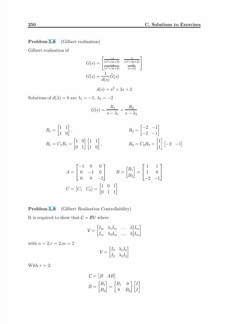
7/28/2019 Control System Theory and Design
http://slidepdf.com/reader/full/control-system-theory-and-design 258/290
250 C. Solutions to Exercises
Problem 5.8 (Gilbert realisation)
Gilbert realisation of
G(s) =
−s(s2+3s+2)
1(s2+3s+2)
−s(s2+3s+2)
−1(s+2)
G(s) =1
d(s)G(s)
d(s) = s2 + 3s + 2
Solutions of d(λ) = 0 are λ1 = −1, λ2 = −2
G(s) =R1
s − λ1
+R2
s − λ2
R1 =
1 1
1 0
, R2 =
−2 −1
−2 −1
R1 = C 1B1 =
1 0
0 1
1 1
1 0
, R2 = C 2B2 =
1
1
−2 −1
A = −1 0 0
0 −1 0
0 0 −2
B = B1
B2
= 1 1
1 0
−2 −1
C =
C 1 C 2
=
1 0 1
0 1 1
Problem 5.9 (Gilbert Realisation Controllability)
It is required to show that C = BV where
V =I m λ1I m . . . λ21I m
I m λ2I m . . . λ22I m
with n = 2,r = 2,m = 2
V =
I 2 λ1I 2I 2 λ2I 2
With r = 2:
C =
B AB
B =
B1
B2
=B1 0
0 B2
I I

7/28/2019 Control System Theory and Design
http://slidepdf.com/reader/full/control-system-theory-and-design 259/290
C.5. Solutions to Chapter 5 251
A = λ1I 0
0 λ2I AB =
λ1B1
λ2B2
=
B1 0
0 B2
λ1I
λ2I
B =
B1 0
0 B2
V has full rank so the system is controllable if and only if B has full rank.
B1 has full rank, B2 has full rank as these are conditions from the Gilbert realisation.
Because of the block diagonal structureB
also has full rank. HenceC
has full rank. A
similar argument can be used to show observability.
Problem 5.10 (Turbogenerator LQR)
a) Let x =
x p xI
. Then y = Cx p
k1(y21 + y2
2) = k1
y1 y2
y1y2
= k1xT
p C T Cx p
k2(x25 + x26) = k2xT I xI
so
k1(y21 + y22) + k2(x2
5 + x26) = k1xT
p C T Cx p + k2xT I xI
=
xT p xT
I
k1C T C 0
0 k2I 2
x p
xI
Q =
k1C T C 0
0 k2I 2
k3(u21 + u2
2) = k3
u1 u2
u1
u2
R = k3I 2
i) Greater weight on state errors: faster response
ii) Greater weight on integrated errors: quicker return to setpoint
iii) Greater weight on inputs: slower response
These are rules of thumb, which have to be considered carefully. Increasing the
weight on one cost means decreasing the weight on the other costs. Thus increasing

7/28/2019 Control System Theory and Design
http://slidepdf.com/reader/full/control-system-theory-and-design 260/290
252 C. Solutions to Exercises
k1 with fixed k2 and k3 can also lead to a slower response. In this case, the weight
on the state errors would be increased, which means, the weight on the integrated
errors and the inputs would be decreased. If the decreasing effect on the weight
on the integrated error is stronger, then the response would be slower. To be sure,
that the response will become faster, the weight on the input should be decreased,
in which case all effects would lead to a faster response.
Only ratios between weights affect the resulting controller. So any one of the three
constants could be fixed to one without loss of generality.
c,d) See cs5_tgen_LQR, cs5_tgensfmod2.mdl, cs5_tgen_LQR_plot.m. Suitable values
of the tuning parameters are k2 = 10, k3 = 0.001.
d) Easier to set weights than to set pole placement positions.
Problem 5.11 (Right half plane zero constraints)
a) From the Smith-McMillan form (or the Matlab commands zero and pole: see
cs5_rhand_zeros.m)
Pole:
−2,
−1,
−2,
−1
Zeros: +0.75
b) Definition of zero: G(s) loses rank at s = z i
G(z i)uzi = 0
G(z i) does not have full rank, so nor does GT (z i). So there must exist a yzi, such
that
G
T
(z i)yzi = 0yT
ziG(z i) = 0
There is only one zero at s = 0.75
G(0.75) =1
(0.5 · 0.75 + 1)(0.75 + 1)
2 1
1 + 4 · 0.75 2
=
0.8312 0.4156
1.6623 0.8312
yzi = k
· −0.8944
0.4472 The singular value decomposition can be used to calculate yzi see cs5_rhand_zeros.m

7/28/2019 Control System Theory and Design
http://slidepdf.com/reader/full/control-system-theory-and-design 261/290
C.5. Solutions to Chapter 5 253
c) The opposite of the condition is
yT ziG(z i)K (z i)
= 0
and this can only be true if K (z i) = ∞, which is exactly when z i is a pole of K (s).
But K (s) cannot have unstable poles which the corresponding zeros of G(s) could
cancel.
d) Pole condition follows directly from definition of internal stability.
The opposite of the condition is
yT ziG(z i)K (z i)1 + G(z i)K (z i)
−1 = 0
which could only be true if 1 + G(z i)K (z i)
−1= ∞
that is, z i is a Pole of
1 + G(z i)K (z i)−1
.
But (1 + K (s)G(s))−1 cannot have poles in the right half plane due to internal
stability requirement. Therefore
yT ziG(z i)K (z i)1 + G(z i)K (z i)
−1= 0
e) Let yzi =
yzi1 yzi2
T
yzi,1 yz2,2
T 11 T 12T 21 T 22
= 0
yzi1T 11(z i) + yzi2T 21(z i) = 0
yzi1T 12(z i) + yzi2T 22(z i) = 0
α1 = −0.08944, α2 = 0.4472
Problem 5.12 (Second question on RHP zero constraints)
a) For setpoint tracking: T (0) = I
T 11(0) = 1, T 12(0) = 0
T 21(0) = 0, T 22(0) = 1
b) For no interaction:T 12(s) = 0, T 21(s) = 0

7/28/2019 Control System Theory and Design
http://slidepdf.com/reader/full/control-system-theory-and-design 262/290
254 C. Solutions to Exercises
c) The conditions to be fulfilled are
yz1T 11(z i) = 0, T 12(0) = 0
T 11(0) = 1
T 21(0) = 0, yz1T 22(z i) = 0
T 22(0) = 1
By inspection T 1(s) does not fulfill this constraint but T 2(s) does.
Valid transfer functions always have an inverse response: the open loop unstable
poles are also apparent in the closed loop if we want to fulfill the decoupling and
steady state conditions. Similar limitations will always apply for any complementary
sensitivity function.
Problem 5.13 (Multivariable controllability form)
a) w1 = S (s)v, w2 = ψ(s)v
G0(s) = ψ(s)S −1(s)
b)
ψ(s) =
s 0
1 0
0 s2
0 s
0 1
S (s) =
s2 0
0 s3
, S −1(s) =
1
s20
0 1s3
G0(s) =
1s
01
s20
0 1s
0 1s2
0 1s3
c) One solution:
y = N (s)v
y = N lψ(s)vN (s) = N lψ(s)

7/28/2019 Control System Theory and Design
http://slidepdf.com/reader/full/control-system-theory-and-design 263/290
C.5. Solutions to Chapter 5 255
N (s) = s 0
−s s2 , ψ(s) =
s 0
1 0
0 s2
0 s
0 1
s 0
−s s2
=
n11 n12 n13 n14 n15
n21 n22 n23 n24 n25
s 0
1 0
0 s2
0 s
0 1
with
N l = 1 0 0 0 0−1 0 1 0 0
N lψ(s) =
1 0 0 0 0
−1 0 1 0 0
s 0
1 0
0 s2
0 s
0 1
=
s 0
−s s2
d) from G0(s):
y1
= u1, y
2= u
1y3 = u2, y4 = u2,
...y 5 = u2
so
x2 = x1
x4 = x3, x5 = x4
and
y1 = x1, y2 = x2, y3 = x3, y4 = x4, y5 = x5
A =
0 0 0 0 0
1 0 0 0 0
0 0 0 0 0
0 0 1 0 0
0 0 0 1 0
, B =
1 0
0 0
0 1
0 0
0 0
C = I 5×5
e)
A = A0 − B0D−1h Dl
B = B0D−1h
C = N l

7/28/2019 Control System Theory and Design
http://slidepdf.com/reader/full/control-system-theory-and-design 264/290
256 C. Solutions to Exercises
Problem 5.14 (Closed loop with MV controllability form)
Matlab solution: cs5_MCctrb.m
c)
hi = ψ(λi) pi
y1y2y3y4y5
=
m11 m12
m21 m22
m31 m32
m41 m42
m51 m52
x1
x2
x1
x2
is ALy (AL is the left inverse of A).
Matlab: p(:,ind)=pinv(psi)*h(:,ind);
pT
1...
pT 5
=
−0.0537 + 0.0985i 0.0102 + 0.0191i
−0.0537 − 0.0985i 0.0102 − 0.0191i
0.0592 − 0.1399i 0.0210 + 0.0280i
0.0592 + 0.1399i 0.0210 − 0.0280i
0.0400 0.2173
Problem 5.15 (Turbogenerator LQG)
The Matlab solution is given in cs5_tgen_LQG.m (cs5_tgen_LQG_plot.m)
a) The setpoint responses are unaffected by the observer, as the observer sees the same
inputs as the plant if d = 0.
As R is increased this is equivalent to the noise at the output increasing in intensity,
which requires ’more’ filtering, that is filtering with a lower bandwidth. This isassociated with a lower gain Kalman filter and slower associated poles.
An alternative interpretation is that as R increases the intensity of the state noise
reduces, so the quality of the estimate in the observer improves, so less correction
by the error y − ye is needed,which in turn requires lower L.
As increasing R makes the filter less responsive to state noise, larger errors are
expected when disturbances enter the states, as they do with the disturbance d.
However, the filter is better at filtering output noise, so a reduction in noise at the
plant input and plant output is expected.
b) Suitable values are for example re1 = 1000, re2 = 1000.

7/28/2019 Control System Theory and Design
http://slidepdf.com/reader/full/control-system-theory-and-design 265/290
C.5. Solutions to Chapter 5 257
c) Construct the required transfer functions (e.g., with linmod) and use the Matlab
function sigma to obtain the singular value plots.
Note in particular:
The closed loop frequency response from r to y has a gain of 0dB at low frequencies,
corresponding to high open loop gain.
The closed loop frequency response to noise is greater than 1 at low frequencies, but
this is probably not a problem as noise is usually high frequency.
In general: At high frequencies the open loop with a break at p1 , L(s)(equivalent to
G(s)K (s)) is close to the complementary sensitivity function as (I +L(s)) ≈ I ; while
the sensitivity function at low frequencies is close to L−1(s) as (I + L(s)) ≈ L(s).
Problem 5.16 (Multivariable vs SISO robustness)
a) Calculation of G(s):
G(s) = C (sI − A)−1B
=
1 10
−10 1
s −10
10 s −1
=1
s2 + 100
s − 100 10(s + 1)
−10(s + 1) s − 100
(may be done by hand or with Matlab)
b) with the inputs to G(s) being w1 and w2 (in either closed loop or open loop),
y1 = g11w1 + g12w2, y2 = g21w1 + g22w2
With Channel 2 in closed loop
w2 = −y2
y2 =g21
1 + g22w1
z 1 = −y1 = −g11w1 + g12y2
= −g11w1 +g12g21
1 + g22w1
after some algebra
z 1
=−
1
sw1
Similarly, with Channel 1 in closed loop z 2 = −1s
w2

7/28/2019 Control System Theory and Design
http://slidepdf.com/reader/full/control-system-theory-and-design 266/290
258 C. Solutions to Exercises
c) The transfer functions with one loop closed are just integrators: Gain margin: ∞Phase margin: 90o
Would therefore expect good robustness in the individual channels.
d) The plant inputs are disturbed by errors 1, 2; with 10 = a,
u1 = (1 + 1)u1, u2 = (1 + 2)u2
B =
1 + 1 0
0 1 + 2
Acl = A − BC
= 0 a−a 0− 1 + 1 0
0 1 + 2 1 a−a 1
=
−(1 + 1) −a1a2 −(1 + 2)
e) Characteristic polynomial of A()cl:
s2 + (2 + 1 + 2)s + 1 + 1 + 2 + (a2 + 1)12
For stability both coefficients must be positive
With 2 = 0: Stable with 1 > −1
With 1 = 0: Stable with 2 > −1
f ) With 2 = −1 = −, for stability need
1 − (a2 + 1)2 > 0
<1√ 101
g) The interpretation of this is that robustness is very good with errors with ’direction’
1 = 2 or 1, 2 = 0 but is not good for the direction 1 = −2.
The conclusion of this is: simple SISO open loop measures of robustness are not a
good guide to MIMO robustness.

7/28/2019 Control System Theory and Design
http://slidepdf.com/reader/full/control-system-theory-and-design 267/290
C.6. Solutions to Chapter 6 259
C.6 Chapter 6
Problem 6.1 (Simple discrete time responses from z transforms)
a)
G(z ) =2z 2 − 6z
2z 2 − 6z + 4
G(z ) =2 − 6z −1
2 − 6z −1 + 4z −2
G(z ) = 1z 0 + 0z −1
−2z −2
−6z −3
−14z −4 . . .
The response is 1,0,-2,-6,. . .
b)
G(z ) =1
1 − 2z −1
with input
u(k) = 2e−kσ(k)
U (z ) =2z
z − e−1
G(z )U (z ) =2z
(1 − 2z −1)(z − e−1)
=2z 2
(z − 2)(z − e−1)= 2 +
4.736z − 1.472
(z − 2)(z − 0.368)
= 2 +a1
z − 2+
a2
z − 0.368
a1 = 4.902, a2 = −0.166
From Z [σ(k)αk] = 11−αz−1 ,
Z [σ(k − 1)αk−1] =1
z − α
so
y(0) = 2
y(k) = 4.9 · 2k
−1
− 0.166 · 0.368k
−1
, k ≥ 1

7/28/2019 Control System Theory and Design
http://slidepdf.com/reader/full/control-system-theory-and-design 268/290
260 C. Solutions to Exercises
Problem 6.2 (Discrete time final value theorem)
x(∞) = limz
→1(z − 1)X (z )
Proof:
Z
x(k)
= X (z ) =∞
k=0
x(k)z −k
Z
x(k − 1)
= z −1X (z ) =∞
k=0
x(k − 1)z −k
∞
k=0x(k)z −k −
∞
k=0x(k − 1)z −k = X (z ) − z −1X (z )
limz→1
∞k=0
x(k)z −k −∞
k=0
x(k − 1)z −k
= lim
z→1
X (z ) − z −1X (z )
with x(k) = 0 when k < 0, and when the system is stable the left hand side becomes
limz→1
∞k=0
x(k)z −k − x(k − 1)z −k
= [x(0) − x(−1)] + [x(1) − x(0)] + [x(2) − x(1)] + . . .
= limk→∞
x(k)
so
limk→∞
x(k) = limz→1
X (z ) − z −1X (z )
= lim
z→1
(z − 1)X (z )
Problem 6.3 (Root loci for discrete systems)
a) i) Lines of constant real part of continuous poles σ: σ = −0.1T
, −0.5T
and −1.0T
.
The line in the z -plane is defined by z = esT = e(σ+ jω)T ;
with σ = −0.1T
:
z = eσT + jωT = eσT e jωT
= e−0.1(cos ωT + j sin ωT )
as ω : 0 → 2πT
a circle is described, with radius e−0.1. Larger magnitude σ
correspond to smaller radiuses.
ii) Lines of constant imaginary parts ω of continuous poles ω = 0.5 πT
, 1.0 πT
and
1.5 πT
.
The line in the z-plane is z = esT . With ω = 0.5 πT
:
z = eσT + jωT
= eσT
e jωT
= eσT (cos0.5π + j sin0.5π)

7/28/2019 Control System Theory and Design
http://slidepdf.com/reader/full/control-system-theory-and-design 269/290
C.6. Solutions to Chapter 6 261
b) Second order system with damping factor ζ and natural frequency ωn. Lines for
ζ = 0, 0.5, 1 as ωn : 0 → πT
.
s = ±ζωn + jωn 1 − ζ 2
with ζ = 0, circle radius is 1.0:
z = eσT + jωT
= (cos ωn + j sin ωn)
In general with k =
1 − ζ 2
z = eσT + jωT
= e−ζωnT (cos kωnT + j sin kωnT )
when ωn : 0 → πT
starting radius is 1.0, final radius is e−πζ .
c) For the second order system, lines for ωn = π2T
, πT
as ζ : 0 → 1.
With ωn = π2T
z = eσT + jωT
= e−ζ π2 cos kπ
2
+ j sin kπ
2with ζ = 0, angle = 90o and Radius=1.0
with ζ = 1, angle = 0o, radius = e−π2
With ωn = πT
:
with ζ = 0, angle = 180o and Radius=1.0
with ζ = 1, angle = 0o, Radius = e−π
These can easily be drawn using the Matlab command rltool with grid.
Problem 6.4 (Discrete time controller form)
z transform:
Y =b1z −1 + b2z −2 + b3z −3
1 + a1z −1 + a2z −2 + a3z −3U
=b1z 2 + b2z 1 + b3
z 3 + a1z 2 + a2z + a3U
Use new variable X 1(z ), so that
(z 3
+ a1z 2
+ a2z + a3)X 1 = U Y = b1z 2X 1 + b2zX 1 + b3X 1

7/28/2019 Control System Theory and Design
http://slidepdf.com/reader/full/control-system-theory-and-design 270/290
262 C. Solutions to Exercises
with
X 2 = zX 1
X 3 = zX 2
zX 3 = z 3X 1 = −a1X 3 − a2X 2 − a3X 1 + U
Y = b1X 3 + b2X 2 + b3X 1
The state space Z transform model is
zX = AX + BU
Y = CX + DU
A =
0 1 0
0 0 1
−a3 −a2 −a1
, B =
0
0
1
C =
b3 b2 b1
D = 0
or, in the discrete time domain
x(k + 1) = Ax(k) + Bu(k), y(k) = Cx(k) + Du(k)
See Figure C.3
y
z −1
−a1
z −1
−a2 −a3
z −1 b3
b2
b1
ux2x3 x1
Figure C.3: discrete time controller form

7/28/2019 Control System Theory and Design
http://slidepdf.com/reader/full/control-system-theory-and-design 271/290
C.6. Solutions to Chapter 6 263
Problem 6.5 (Discrete time proportional controller)
a) Root locus has a single pole at −a.
b) Continuous time state space model of the system is given as,
x = −ax + bu,
y = x
Let it’s discrete time state space representation be given as,
zx = Φx + Γu, y = x
where,
Φ = e−aT , Γ =
T
0
e−atbdt
= [e−at
−a]T 0 b
=(1 − e−aT )
ab
Then,
Y (z ) = C (zI − Φ)−1Γ = Γz − Φ
= ba
1 − e−aT
z − e−aT
c) The discrete root locus has a pole at z = e−aT = 0.67
G(z ) =b
a
1 − e−aT
z − e−aT =
1
2
1 − 0.67
z − 0.67=
0.16
z − 0.67
so the characteristic equation in closed loop 1 + K (z )G(z ) = 0 is
1 + K (z )G(z ) = 0
1 + K pd0.16
z − 0.67= 0
z − 0.67 + 0.16K pd = 0
The root locus is on the real axis, so the system becomes unstable when it hits the
unit circle at z = −1: K pd = 10.44.
d) The continuous proportional controller is always stable: the closed loop pole tends
to s = −∞. As shown in c), this is not true for the discrete controller.
e) See Matlab/Simulink cs6_discrete_P.m and cs6_discrete_P_mod.mdl

7/28/2019 Control System Theory and Design
http://slidepdf.com/reader/full/control-system-theory-and-design 272/290
264 C. Solutions to Exercises
Problem 6.6 (Discrete time PD controller)
a) The continuous time state space model is given as,x = Ax + bu,
y = x
where,
A =
0 1
0 0
, b =
0
1
, c =
1 0
.
Let the discrete time state space representation be given as,
zx = Φx + Γu, y = x
where,
Φ = eAT , Γ =
T
0
eAtBdt
Then, Φ and Γ can be approximated by using the Taylor series as,
Φ = I + AT +
A2T 2
2 + . . . , Γ = A−1
(eAT
− I )B
= A−1(AT +A2T 2
2+
A3T 3
3!+ . . .)B
= (T +AT 2
2+
A2T 3
3!+ . . .)B
Since,
A2 = 0
we have,Φ = I + AT =
1 T
0 1
, Γ = (T +
AT 2
2)B
Γ =
T 0
0 T
+
0 1
0 0
T 2
2
0
1
=
T 2/2
T
G2(z ) = C (zI − Φ)−1Γ
=
1 0
z
1 0
0 1
−
1 T
0 1
−1 T 2/2
T
= T 2
2z + 1
(z − 1)2

7/28/2019 Control System Theory and Design
http://slidepdf.com/reader/full/control-system-theory-and-design 273/290
C.6. Solutions to Chapter 6 265
b) Continuous RL (continuous controller):
Two Poles at (0, 0); RL is always on the imaginary axis.
Discrete RL (discrete controller):Two poles at z = 1, zero at z = −1;
RL is a circle with radius > 1: see cs6_discrete_PD.m. The system is always
unstable.
c)
C 2(z ) = K pd
1 + T d(1 − z −1)
= K pd
1
z
(1 + T d)z − T d
= K pd
1 + T dz
z − T d1 + T d
α =T d
1 + T d,
1
1 − α= 1 + T d
d) See cs6_discrete_PD.m. To assist the design in rltool right-click over the root-
locus, chose Properties , Options and select Show grid . One solution is Kpd=12.4,
alpha=0.83.
e) Kpd=2.08, alpha=0.83 is one solution.
A solution as fast as that in (d) is not possible; design in the discrete time domain
tells us explicitly what limitations arise as we increase the sampling time.
Problem 6.7 (Deadbeat controller design )
The command acker can be used to place the poles on the origin. If acker is not provided
with the Matlab version, one can use also place, by positioning the poles close to the
origin, e.g. [0, 1e-5] (place does not allow several pole on the same location”). The
solution is in cs6_deadbeat.m and cs6_deadbeat_sim.mdl.
As expected, the steady state is reached after precisely two sampling periods.
Problem 6.8 (Discrete turbogenerator)
a) This can be done in two steps:
step 1) generate state space representation of complete controller. This can be done
using linmod()
step 2) use c2d() to get discrete time approximation.
b) The simulation shows that:
– for controller discretised with T = 0.02 the controlled response is almost iden-
tical.

7/28/2019 Control System Theory and Design
http://slidepdf.com/reader/full/control-system-theory-and-design 274/290
266 C. Solutions to Exercises
– for controller discretised with T = 0.5 the controlled response is notably dif-
ferent because of large sampling time.
c) See cs6_TG_discrete_K.m.
d) The response of closed loop systems are notably different then the one achieved by
approximating the continuous time controllers by Tustin approximation. This is
because same weighting matrices Q, R, Qe and Re are used in both the cases. This
is not the correct approach if one wants to design discrete time controllers to achieve
same performance as achieved by continuous time controllers. It can be shown that
to achieve same performance, one needs to modify the weighting matrices. This
even requires modification in cost function J by including cross terms of the form
x(kT )Su(kT ) in its discrete counterpart.
e) The response of continuous time model with time delay of 0.25 s resembles that of
the discretised controller with sampling time 0.5 s. This is particularly clear in the
first several samples after the step disturbance is applied. This shows that the effect
of Tustin approximation with sampling time T is similar to the effect of adding a
time delay T /2 to the original system.
Problem 6.9 (Discrete convolution)
Since,
G(z ) = Y (z )U (z )
Then,
Y (z ) = G(z )U (z )
from definition of z -transform∞
k=0
y(k)z −k =
∞k=0
g(k)z −k
∞k=0
u(k)z −k
y(0) + y(1)z −1 + y(2)z −2 + . . . = (g(0) + g(1)z −1 + g(2)z −2 + . . .)(u(0)
+u(1)z −1
+ u(2)z −2
+ . . .)= g(0)u(0) + (g(0)u(1) + g(1)u(0))z −1 +
(g(0)u(2) + g(1)u(1) + g(2)u(0))z −2 + . . .
Comparing coefficients of (z 0, z −1, z −2, . . .) we get,
y(0) = g(0)u(0)
y(1) = g(0)u(1) + g(1)u(0)
y(2) = g(0)u(2) + g(1)u(1) + g(2)u(0)...
y(k) =k
l=0
g(l)u(k − l)

7/28/2019 Control System Theory and Design
http://slidepdf.com/reader/full/control-system-theory-and-design 275/290
C.6. Solutions to Chapter 6 267
Problem 6.10 (Impulse response)
a) The impulse response can be easily computed by the so-called Markov parameters:
g(0) = D = 0
g(1) = C Γ = 1
g(2) = C ΦΓ = 4.2
g(3) = C Φ2Γ = 0.84
b) The response to a particular input can be computed using the discrete convolution
formula: y(k) =
kl=0 g(l)u(k − l)
y(0) = g(0)u(0) = 0
y(1) = g(0)u(1) + g(1)u(0) = 0 + 5 = 5
y(2) = g(0)u(2) + g(1)u(1) + g(2)u(0) = 0 + 0 + 21 = 21
y(3) = g(0)u(3) + g(1)u(2) + g(2)u(1) + g(3)u(0) = 0 − 1 + 0 + 4.2 = 3.2
Problem 6.11 (Zeros of discrete time system)
a) i)
G(s) =s + 1
s2 + 4s + 1
n = 2, m = 1, n − m − 1 = 0
For this system there is one continuous zero s = −1.
The discretisation results in only one zero, and it approaches e−T .
ii)
G(s) =
1
s3 + s2 + sn = 3, m = 0, n − m − 1 = 2
The discretisation of this system results in two zeros: they approach the zeros
of the exact discretisation 1/s3, so we need the exact discretisation of 1/s3.
A state space representation of 1/s3 is(using that...x = u)
x1 = x2
x2 = x3
x3 = u
A =
0 1 0
0 0 1
0 0 0
, B =
0
0
1
y = x1 C =
1 0 0

7/28/2019 Control System Theory and Design
http://slidepdf.com/reader/full/control-system-theory-and-design 276/290
268 C. Solutions to Exercises
Discretisation
Φ = eAT = I + AT +A2T
2+ . . .
A2 =
0 0 1
0 0 0
0 0 0
, A3 = 03×3
Φ =
1 T T 2/2
0 1 T
0 0 1
Ψ = 1 +AT
2+
A2T 2
3!=
1 T 2
T 2
6
0 1 T
20 0 1
Γ = ΨT B =
T 3
6T 2
2
T
Let, z be a zero of
x(k + 1) = Φx(k) + Γu(k)
y(k) = Cx(k)
then, (zI − Φ) −Γ
C D
x
u
= 0
Since, D = 0, so we have Cx = 0
1 0 0
x1
x2
x3
= 0, ⇒ x1 = 0, x =
0
x2
x3
First row: u = 1, (zI − Φ)x − Γu = 0
z − 1 −T −T 2/2
0 z − 1 −T
0 0 z − 1
0
x2
x3
−
T 3
6T 2
2
T
= 0
It then follows that
x3 =T
z
−1
(third row)
x2 = T 2− 1
6− 1
2(z − 1)
(first row)

7/28/2019 Control System Theory and Design
http://slidepdf.com/reader/full/control-system-theory-and-design 277/290
C.6. Solutions to Chapter 6 269
and finally, after substituting in the second row
z 2 + 4z + 1 = 0, z =
−2
±
√ 3
Therefore the zeros of the discretisation of G(s) approach the values −3.73 and
−0.268.
For a minimum phase system |z i| < 1.
If T is reduced, the zeros become closer and closer to the unit disk.
b) When T >≈ 3.3 the system becomes minimum phase.
Problem 6.12 (Finite word length)
The poles of a system (controller or plant) approach +1, as T → 0 (from z = esT ).
As an example, the poles z = 0.9996, z = 0.9998 are not equal to the pole z = 0.9999,
and the three have very different behaviours with T = 0.0001. With this sample time
of T = 0.0001 and a word-length that allows precision up to the third decimal place the
poles would have an identical representation. Finite word-length can be a problem at
any sampling time, but the quicker the sampling time the more sensitive the implemented
pole positions become to their finite word length representation. With a finite word-length
the real implemented poles can lie a long distance from the required poles, making theperformance of the closed loop different from that designed.
Finite word-length can lead to an additional problems in the digital systems due to quan-
tization effects - during sampling the continuous time signals they are converted to a
digital signal, that can take only a finite number of values, for example for N=8 bit word-
length, the signal can take only values between 0 and 255. If the original signal is Y
between, e.g., −5 and 5 V, then the quantized signal can take only values with a step of
q = (Y max − Y min)/(2N − 1) = 10/255 = 0.0392 V/bit. Big quantization steps can lead to
loss of performance and even instability. The effect of quantization can be simulated in
Simulink using the Quantizer block.
Problem 6.13 (Sampling times)
a) The time constant τ = 5 sec, the bandwidth is ωb = 0.2 rad/s and the gain is 1.
b) Attenuation of 3 dB occurs at the system’s bandwidth, therefore ω3 = ωb = 0.2
rad/s.
c) To avoid aliasing effect the sampling frequency should be ωs > 2ωb. If we chose
ωs = 10ωb = 2 rad/s, then the sampling time is T s = 2π/ωs = 3.14 sec. Therefore
sampling times smaller than 3.14 sec. are suitable.

7/28/2019 Control System Theory and Design
http://slidepdf.com/reader/full/control-system-theory-and-design 278/290
270 C. Solutions to Exercises
Problem 6.14 (Frequency response of zoh unit)
a) y(t) as a function of u(t) at the sample times u(kT ):Use the pulse function σ(t − nT ) − σ
t − (n + 1)T
.
The functions
σ(t) − σ(t − T )
σ(t − T ) − σ(t − 2T )
σ(t − 2T ) − σ(t − 3T )
are shown below on Figure C.4. The y(t) is shown on Figure C.5.
σ(t) − σ(t − T )
0 2T T
σ(t − 2T ) − σ(t − 3T )
σ(t − T ) − σ(t − 2T )
3T
Figure C.4: Series of pulses of width T superimposed
Mathematically y(t) is
y(t) = u(0)
σ(t) − σ(t − T )
+ u(T )
σ(t − T ) − σ(t − 2T )
+ u(2T )
σ(t − 2T ) − σ(t − 3T )
+ . . .
=
∞k=0
u(kT )σ(t − kT ) − σt − (k + 1)T b) Laplace Transformation of y(t): u(kT ) are constant multipliers.
The Laplace transform of σ(t − kT ) − σ
t − (k + 1)T
is
L
σ(t − kT )
=e−kT s
s
Lσt − (k + 1)T =e−(k+1)T s
s
L
σ(t − kT ) − σ
t − (k + 1)T
=e−kT s − e−(k+1)T s
s

7/28/2019 Control System Theory and Design
http://slidepdf.com/reader/full/control-system-theory-and-design 279/290
C.6. Solutions to Chapter 6 271
u(2T )
0 2T T
u(t)
y(t)
3T
u(0)
u(T )
Figure C.5: Input and output of sampler
As u(kT ) are just constant multipliers the following holds:
Y (s) = L
y(t)
=∞
k=0
u(kT )e−kT s − e−(k+1)T s
s
=1 − e−T s
s
∞k=0
u(kT )e−kT s
c) u∗(t) is a sequence of δ pulses
L
u∗(T )
= u(T )e−T s (1 Pulse)
U ∗(s) = L
u∗(t)
=∞
k=0
u(kT )e−kT s (all Pulses)
So it follows that
Y (s) =1 − e−T s
sU ∗(s)
That is, the transfer function of the sampler Gzoh is
Gzoh =Y (s)
U ∗(s)=
1 − e−T s
s
d) The frequency response of Gzoh is
Gzoh( jω) =1 − e−T jω
jω
=T
ωT /2
eT 2 jω − e−
T 2 jω
2 j
e−0.5T jω
= T sin(ωT /2)ωT /2
e−0.5T jω

7/28/2019 Control System Theory and Design
http://slidepdf.com/reader/full/control-system-theory-and-design 280/290
272 C. Solutions to Exercises
Bode Diagram:
Gzoh( jω) = E ( jω)F ( jω), E ( jω) = T sin(ωT /2)
ωT /2, F ( jω) = e−0.5T jω
|E (0)| = T,
E
2nπ
T
= 0, |F ( jω)| = 1 ∀ω
E ( jω) = 0, 0 < ω < 2π/T, 4π/T < ω < 6π/T, . . .E ( jω) = 180(= −180), 2π/T < ω < 4π/T, 6π/T < ω < 8π/T, . . .F ( jω) = −0.5T ω
Every 2nπT
the sign of E ( jω) changes. G( jω) experiences at these values a further
phase shift of ±180.
Matlab: cs6_S_and_H.m
Problem 6.15 (Frequency response of discrete system with sinusoidal input)
a) Calculation of u∗(t) when u(t) = sin ωt:
u∗(t) = sin(ωt)∞
k=−∞
δ (t−
kT )
using the hint
u∗(t) = sin(ωt)1
T (1 + 2 cos ωst + 2 cos 2ωst + . . .)
b) The Delta sampler is not a linear system! It is actually a modulator.
We can calculate the output of the modulator using a Fourier transform (not a
transfer function).
The zero order hold is linear, so it has a transfer function, and its frequency responsecan be used to describe its behaviour.
Interpretation
Using the trigonometric formulae
2sin α cos β = sin(α + β ) − sin(β − α)
sin α + sin β = 2 sinα + β
2cos
β − α
2
With the sample time T = 0.05s
ωs = 2π/T = 125.6 rad/s

7/28/2019 Control System Theory and Design
http://slidepdf.com/reader/full/control-system-theory-and-design 281/290
C.6. Solutions to Chapter 6 273
With an input frequency ω = 2 rad/s
u∗(t) = 20sin(2t)(1 + 2 cos 125.6t + 2 cos 251.2t + . . .), (α = 2, β = 125.6)
u∗(t) = 20sin(2t) + 20 sin(125.6 + 2)t − 20 sin(125.6 − 2)t + . . .
y(t) = G( j2)Gzoh( j2)u∗(t)
y(t) ≈ 20G( j2)Gzoh( j2) sin(2t)
After the zero order hold zoh and G(s) (which act as filters) only the first elements
are large.
With the input ω = 60rad/s
u∗(t) = 20 sin(60t)(1 + 2 cos 125.6t + 2 cos 251.2t + . . .)
= 20 sin(60t) + 20 sin(125.6 − 60)t − 20 sin(125.6 + 60)t + . . .
α = 60, β = 65.6,α + β
2= 62.8,
β − α
2= 2.8
y(t) ≈ 20G( j60)Gzoh( j60)sin62.8t cos2.8t
The first two frequencies are similar: similar amplification by Gzoh(s)G(s). Because
of this we get the phenomena of ’beating’- a low frequency variation of amplitude.

7/28/2019 Control System Theory and Design
http://slidepdf.com/reader/full/control-system-theory-and-design 282/290
274 C. Solutions to Exercises
C.7 Chapter 7
Problem 7.1 (Proof of least squares optimality)
Using the approach of completion of squares:
Let
V ( p) = (Y − Mp)T (Y − Mp)
= Y T Y − pT M T Y − Y T Mp + pT M T Mp
or
V ( p) − Y T Y = pT M T Mp − pT M T Y − Y T Mp
Adding a constant term Y T M (M T M )−1M T Y to both side will yield,
V ( p) − Y T Y + Y T M (M T M )−1M T Y = pT M T Mp − pT M T Y − Y T Mp
+Y T M (M T M )−1M T Y
= ( p − (M T M )−1M T Y )T M T M ( p − (M T M )−1M T Y )
Thus,
V ( p) = ( p− (M T M )−1M T Y )T M T M ( p− (M T M )−1M T Y ) + Y T Y −Y T M (M T M )−1M T Y
Which shows that V ( p) is minimum if the first term on right hand side is minimum or
equal to zero. Then,
p − (M T M )−1M T Y = 0
or
p = (M T M )−1M T Y
Thus ˆ p = p = (M T M )−1M T Y ) that minimizes V ( p).
Problem 7.2 (Persistent excitation of step and white noise)
a)
(z − 1)u(kT ) = u(kT + T ) − u(kT )
For the step function u(t + T ) − u(t) is only 1 at k = −1.
b) If, for all polynomials a(z ) of order n (anz n + . . .):
limk→∞
1k
kl=0
(a(z )u(l))2 > 0

7/28/2019 Control System Theory and Design
http://slidepdf.com/reader/full/control-system-theory-and-design 283/290
C.7. Solutions to Chapter 7 275
the PE order is n + 1.
This means that if any polynomial a(z ) can be found such that
limk→∞
1
k
kl=0
(a(z )u(l))2 = 0
then the PE order must be ≤ n.
c) With the polynomial a(z ) = z − 1 (order n = 1) and u(l) a step function, then from
a).
a(z )u(l) = 0, l = 0, 1, . . . ∞so
limk→∞
1k
kl=0
(a(z )u(l))2 = 0
so the PE order is either 1 or 0.
d) Next, we will find the exact order by analyzing the auto correlation C uu(1) = cuu(0).
Since, it is a scaler hence it has rank of 1 or PE order is 1.
e) For white noise,
C uu(1) = cuu(0) = limk→∞
1
k
k
i=0 u2i
= S 0
C uu(2) =
cuu(0) cuu(1)
cuu(1) cuu(0)
Using, the property of white noise that cuu(i) = 0, ∀i = 1, 2 . . . ,
C uu(2) =
cuu(0) 0
0 cuu(0)
= S 0I 2...
C uu(n) = S 0I n
so C uu(n) has rank n or PE condition is satisfied for all n.
Problem 7.3 (PE of sinusoid)
a)
(z 2 − 2z cos ωT + 1)u(kT ) = sin(ωkT + 2ωT ) − 2cos ωT sin(ωkT + ωT ) + sin(ωkT )

7/28/2019 Control System Theory and Design
http://slidepdf.com/reader/full/control-system-theory-and-design 284/290
276 C. Solutions to Exercises
Since,
sin A + sin B = 2 sinA + B
2
cosA − B
2
sin(ωkT + 2ωT ) + sin(ωkT ) = 2 sin(ωkT + ωT )cos ωT
(z 2 − 2z cos ωT + 1)u(kT ) = 0
b) If we can find any polynomial a(z ) of order n, such that
limk→∞
1
k
kl=0
(a(z )u(l))2 = 0
Then, the PE order must be ≤ nWith a(z ) = (z 2 − 2z cos ωT + 1), i.e. n = 2. As shown in a),
a(z )u(l) = 0, ∀l = 0, 1, . . . ∞
Then,
limk→∞
1
k
kl=0
(a(z )u(l))2 = 0
So the PE order must be ≤ 2.
c) For the input signal u(kT )
Ru(τ ) = limN →∞
1
N
N k=0
u(kT )u(kT ± τ )
At times 0 and T
Ru(0) = limN →∞
1
N
N
k=0u(kT )u(kT )
Ru(T ) = limN →∞
1
N
N k=0
u(kT )u
(k + 1)T
These are the elements (1, 1) and (1, 2) of C 2, so
C uu(2) =
Ru(0) Ru(T )
Ru(T ) Ru(0)
C uu(2) =
12
cos0 12
cos ωT 12
cos ωT 12
cos0
C uu(2) = 12
1 cos ωT cos ωT 1

7/28/2019 Control System Theory and Design
http://slidepdf.com/reader/full/control-system-theory-and-design 285/290
C.7. Solutions to Chapter 7 277
d) At T = 2πω
C uu(2) = 12
cos0 12
cos ωT 1
2cos ωT 1
2cos0 =
0.5 0.5
0.5 0.5rankC uu(2) = 1
So PE order is 1. All the samples are at the same position in the sine wave so it
looks like a step.
At ω = 2πT
, the samples are at different positions in the sine wave, so it has more
information: PE order =2.
Problem 7.4 (Least Squares identification)
a) Let us have N samples and let n = 2 then,
y0 = −a1y−1 − a2y−2 + b1u−1 + b2u−2 + e0
y1 = −a1y0 − a2y−1 + b1u0 + b2u−1 + e1
y2 = −a1y1 − a2y0 + b1u1 + b2u0 + e2
y3 = −a1y2 − a2y1 + b1u2 + b2u1 + e3...
yN −1 = −a1yN −2 − a2yN −3 + b1uN −2 + b2uN −3 + eN −1
or
y0y1...
yN −1
=
−y−1 −y−2 u−1 u−2−y0 −y−1 u0 u−1
......
......
−yN −2 −yN −3 uN −2 uN −3
a1
a2
b1b2
+
e2e3...
eN −1
However, the values of input sequence u(−1), u(−2), ...u(−n), and y(−1), y(−2),
...y(−n) is not available in measurement data. This means that first n-rows will be
0, hence to make M T M full rank these rows should be eliminated. This results in,
M =
−y1 −y0 u1 u0
−y2 −y1 u2 u1...
......
...
−yN −2 −yN −3 uN −2 uN −3
which has the dimensions of N − n × 2n:

7/28/2019 Control System Theory and Design
http://slidepdf.com/reader/full/control-system-theory-and-design 286/290
278 C. Solutions to Exercises
b) See cs7_LSrankM.m.
For the sinusoid: rank = 4 (singular values confirm this).
For the white noise: rank = arbitrary
As the sequence becomes longer, the matrix M T M approaches a scaled version of
the empirical covariance matrix; thus the rank of M T M for a long sequence can be
expected to have the same rank as the PE order.
c) See Matlab solution in cs7_LSparest.m. 3rd and 4th order models generated are
identical. A pole and zero cancel in the 4th order model.
d) Exact validation achieved with these models: the model order is clearly 3.
e) Inconsistent results when attempt to generate models from sinusoidal or step input.A true inverse is only possible when rank M T M = 2n: with a PE order of 2 it is
only possible to accurately estimate a system of order 1 (which has 2 parameters).
Problem 7.5 (Subspace identification)
a) Clear cut-off, 9 non-zero singular values in Hankel matrix. Reasonable model
achieved with model order 4. The model can be estimated using cs7_parest.m
b) The cut-off is not so clear for the noisy signal. Since after the 4th singular value of Hn the others are relative small one can chose 4th or 5th order model. Because the
difference between the 3rd and the 4th singular values is also large one can try also
identifying a 3rd order model of the system.
Problem 7.6 (Subspace identification using ident GUI)
1. Open the toolbox with the command ident.
2. Import the data: Import data → Data object → Object : iodata1. Repeat for thesecond data set.
3. The signals then appear in the left panel Data Views .
4. Drag and drop the first signal set to Working model . Remove the means from all
signals using the Preprocess drop-down list → Remove means . Repeat for the second
signal set. One of the new set of signals should be used as Working data and the
other one as Validation data .
5. Estimate models of 2nd, 3rd, 4th and 5th order using N4SID (subspace identifica-
tion). For the purpose choose Parametric model from the Estimate drop-down box.
Select State-space as Structure and repeat the identification for the different orders.

7/28/2019 Control System Theory and Design
http://slidepdf.com/reader/full/control-system-theory-and-design 287/290
C.8. Solutions to Chapter 8 279
6. Validate the identified models using the second data set. Use the Model Views
check-boxes in the lower-right corner of the GUI.
The model used to create the data was 4th order with noise. The identified models of
order 2-4 all very accurately reproduce the original data.
C.8 Chapter 8
Problem 8.1 (Reduction by truncation and residualization)
a) The functions are in the files balresid.m, baltruncation.m
b) The graphs are generated in the script cs8_HVDC_reduce.m. You can compare your
results to the results obtained using the Matlab function balred.

7/28/2019 Control System Theory and Design
http://slidepdf.com/reader/full/control-system-theory-and-design 288/290
Bibliography
[1] T. Kailath
Linear Systems
Prentice Hall, 1980
[2] G.F. Franklin, J.D. Powell and A. Emami-Naeini
Feedback Control of Dynamic Systems
Addison Wesley, 2002
[3] K. Zhou, J.C. Doyle and K. Glover
Robust and Optimal Control
Prentice Hall, 1996
[4] K.J. Astrom, B. Wittenmark
Computer Controlled Systems
Prentice Hall, 1997
[5] L. Ljung
System Identification - Theory for the User
Prentice Hall, 1999
[6] L. Ljung
System Identification Toolbox For Use with MATLAB - User’s Guide
The MathWorks, 2001
[7] G. Strang
Linear Algebra and its Applications
Third Edition
Harcourt Brace Jovanich College Publishers, 1988
[8] C.D. McGillem
Probabilistic Methods of Signal and System Analysis
Oxford University Press, 1998

7/28/2019 Control System Theory and Design
http://slidepdf.com/reader/full/control-system-theory-and-design 289/290
Exercises Summer Term 2009
No. Date Problem ML Topic
1 29 Oct 1.1 Linearisation tank with valve2009 1.2 State space representations
1.3 Cayley-Hamilton Theorem
2 12 Nov 1.4 ML Phase plane diagrams
2009 1.5 Characteristic Polynomial
1.6 Time response
3 19 Nov 1.7 ML Mass-Spring System
2009 1.8 Observer canonical form
1.9 Similarity transformation
2.1 Analysis of controllability
2.2 Bi-proper system4 26 Nov 2.5 ML Bass-Gura Formula
2009 2.6 Inverted Pendulum
2.7 ML Inverted Pendulum - feedback controller
2.8 Transformation into controller form
5 3 Dec 2.9 PBH test
2009 2.11 Controllability with state feedback
3.1 ML Stabilisability and detectability
3.2 ML Single inverted pendulum with friction
4.1 ML Observer design using Matlab
4.2 ML Zeros of state space model6 17 Dec 4.3 ML Setpoint tracking design with static prefilter
2009 4.4 Observability under state feedback
4.5 ML Setpoint following using integrators
4.6 ML Opt. contr. and observer design with symm. root locus
4.7 Roots of SRL at limits of ρ
5.2 + 5.4 Sensitivity S and complementary sensitivity T
7 17 Dec 5.3 ML Pole placement design for turbogenerator
2009 5.7 ML Kalman decomposition
5.9 Gilbert Realisation Controllability
5.10 ML Turbogenerator LQR5.11 ML Right half plane zero constraints
5.15 ML Turbogenerator LQG
8 14 Jan 6.1 Simple discrete time responses from z transforms
2010 6.2 Discrete time final value theorem
6.3 Root loci for discrete systems
6.4 Discrete time controller form
6.5 ML Discrete time proportional controller
6.6 ML Discrete time PD controller
6.7 ML Deadbeat controller design

7/28/2019 Control System Theory and Design
http://slidepdf.com/reader/full/control-system-theory-and-design 290/290
282 BIBLIOGRAPHY