controllability of a linear dynamical system with random parameters
TRANSCRIPT
ISSN 0012-2661, Differential Equations, 2007, Vol. 43, No. 4, pp. 469–477. c© Pleiades Publishing, Ltd., 2007.Original Russian Text c© Yu.V. Masterkov, L.I. Rodina, 2007, published in Differentsial’nye Uravneniya, 2007, Vol. 43, No. 4, pp. 457–464.
ORDINARY DIFFERENTIAL EQUATIONS
Controllability of a Linear Dynamical Systemwith Random Parameters
Yu. V. Masterkov and L. I. RodinaInstitute of Mathematics and Computer Science, Udmurt State University, Izhevsk, Russia
Received April 12, 2004
DOI: 10.1134/S0012266107040040
INTRODUCTION
Real-life control systems often admit no strict deterministic description owing to various randomfactors affecting their behavior. Therefore, in numerous applied fields, one has to take into accountthe influence of random perturbations on the system in question. In the present paper, we obtainconditions for the existence of a nonanticipating control for a linear system with stationary randomparameters
x = A(f tω
)x + B
(f tω
)u, (t, ω, x, u) ∈ R × Ω × R
n × Rm. (1)
Here (A (f tω) , B (f tω)) is a piecewise constant random matrix. [This means that (A (f tω) , B (f tω))is a step function for each fixed ω.] We also describe an algorithm for constructing a nonanticipatingcontrol. [A control u(t, x) is said to be nonanticipating if its construction at time t = τ is basedonly on the behavior of the system for t ≤ τ .] The notion “nonanticipating control” was introducedby the Yekaterinburg school on control theory [1, 2]. The construction of such a control and thecontrollability of linear systems with random parameters were considered in [3–10].
BASIC DEFINITIONS AND NOTATION
Let us consider the probability space (Ω, F, P ) that is the direct product of two probabilityspaces: (Ω, F, P ) = (Ω1 × Ω2, F1 × F2, P1 × P2). Here Ω1 stands for the space of numerical se-quences θ = (θ1, . . . , θk, . . .), θk ∈ (0,∞), F1 is the least σ-algebra generated by cylindrical setsCk
.= C (I1, . . . , Ik) = {θ ∈ Ω1 : θ1 ∈ I1, . . . , θk ∈ Ik}, Ii.= (ai, bi], and P1 is a probabil-
ity measure defined as follows. For each half-open interval Ii, we define the probability measureP1 (Ii) = Fi (bi) − Fi (ai) via the distribution functions Fi(x), 0 < x < ∞. On the algebra of cylin-drical sets, we construct the measure P1 (Ck) = P1 (I1) P1 (I2) · · · P1 (Ik). Then there exists a uniqueprobability measure P1 on (Ω1, F1) that is a continuation of P1 to the σ-algebra F1 (see [11, p. 176]).
Further,Ω2
.= {ϕ : ϕ = (ϕ0, ϕ1, . . . , ϕk, . . .) , ϕk ∈ Ψ} ,
where Ψ = {ψi}s
i=1 is a finite set of pairs ψi.= (Ai, Bi) of matrices; F2 is the least σ-algebra generated
by the cylindrical sets Gk = Gk (ϕ0, ϕ1, . . . , ϕk), where Gk is the set of all sequences in Ω2 in whichthe first k + 1 coordinates are fixed. Let πi = p0 (ψi) and pij = p (ψi, ψj) be given nonnegativefunctions such that
∑s
i=1 πi = 1 and∑s
j=1 pij = 1. Then we define a measure of the cylindricalset Gk by the relation P2 (Gk) = p0 (ϕ0) p (ϕ0, ϕ1) · · · p (ϕk−1, ϕk) and denote the continuation ofthe measure P2 from the algebra of cylindrical sets to the σ-algebra F2 by P2. On the space(Ω2, F2, P2), we introduce the sequence ζ = (ζ0, ζ1, . . .) of random numbers, where ζk(ϕ) = ϕk,ϕk ∈ Ψ. By [11, p. 122], the sequence ζ forms a homogeneous Markov chain, which is uniquelydetermined by the matrix of transition probabilities Π = (pij)
s
i,j=1 and the initial distributionπ = (πi)
s
i=1. We assume that the Markov chain ζ is stationary (in the narrow sense); i.e.,
P (ζ0 ∈ Ψ0, ζ1 ∈ Ψ1, . . .) = P (ζk ∈ Ψ0, ζk+1 ∈ Ψ1, . . .)
for any k ≥ 1, where Ψ0,Ψ1, . . . ∈ I; and I is the σ-algebra of subsets of Ψ [11, p. 432].
469
470 MASTERKOV, RODINA
We introduce a sequence {τk}∞k=0 as follows: τ0 = 0 and τk(θ) =∑k
i=1 θi, where θ ∈ Ω1. Weassume that θi ∈ (0,∞), i = 1, 2, . . . , are independent random numbers; moreover, θ2, θ3, . . . haveidentical distribution F (t), t ∈ (0,∞), with expectation mθ. Note that the condition θi ∈ (0,∞),i = 1, 2, . . . , implies the existence of δ > 0 such that F (δ) < 1. By ν(t) we denote the number ofpoints of the sequence {τk} lying to the left of t; i.e., ν(t) = max {k : τk ≤ t}, t ≥ 0. The quantityν(t) is referred to as the reconstruction process. We assume that ν(t) is a stationary reconstructionprocess (i.e., that process has a constant reconstruction rate); then the distribution of θ1 is givenby the formula [12, pp. 145–147]
F1(t) =1
mθ
t∫
0
(1 − F (x))dx, t > 0.
On the space (Ω1, F1, P1), we introduce the shift transformation
f t1θ = (τν+1 − t, θν+2, θν+3, . . .) , t > 0.
Since ν(t) is a stationary reconstruction process, it follows that the transformation f t1 preserves the
measure P1. For each θ ∈ Ω1, we set f t2(θ)ϕ = (ϕν , ϕν+1, . . .) on (Ω2, F2, P2). Since the Markov
chain is stationary, it follows that f t2 preserves the measure P2. We have thereby defined dynamical
systems (Ω1, ft1) and (Ω2, f
t2) with continuous time. On the space (Ω, F, P ), we also define the
shift transformation f tω = f t(θ, ϕ) = (f t1(θ), f t
2(θ)ϕ). The dynamical system (Ω, f t) is referred toas a skew product of the dynamical systems (Ω1, f
t1) and (Ω2, f
t2(θ)), and the transformation f tω
preserves the measure P = P1 × P2 [13, p. 190].Let ξ(ω) = ζ0(ω) be a random variable on (Ω, F, P ). We introduce the random variable
ξ(f tω
)= (A
(f tω
), B
(f tω
))
generated by the flow f tω. Then ξ (f tω) takes constant values ϕk for t ∈ [τk, τk+1). The functionξ (f tω) is a stationary (in the narrow sense) random process [11, p. 433; 13, p. 167; 14, p. 68;15, p. 189; 16, p. 13]. Recall that a process ξ(t, ω) is said to be stationary in the narrow sense ifP (f tG) = P (G) for any cylindrical set G ∈ F [13, p. 174].
We identify system (1) with the function ξ : Ω → Ψ. For each fixed ω, the function ξ (f tω)specifies a linear deterministic system. For admissible controls in the system ξ, we take all possiblebounded Lebesgue measurable functions uω : R × R
n × Rn → R
m. Solutions of the system ξcorresponding to a control uω (t, x, x0) are treated in the Filippov sense. A control of the formuω (t, x0) that does not depend explicitly on x is referred to as a program control, and a control ofthe form uω(t, x) is said to be positional. A program control uω (t, x0) is said to be nonanticipatingon an interval [t0, t1] if the construction of uω (t, x0) at each time τ ∈ [t0, t1] is performed on thebasis of information on the matrices A (f tω) and B (f tω) only for t ≤ τ (rather than informationfor t > τ).
A state x0 ∈ Rn of the system ξ (f tω) is said to be controllable (respectively, nonanticipatingly
controllable) on [t0, t1] if there exists a control uω (t, x, x0) [respectively, a nonanticipating controlu (f tω, x, x0)], t ∈ [t0, t1], such that the corresponding solution x(t, ω), x (t0, ω) = x0, satisfies thecondition x (t1, ω) = 0.
Let ω ∈ Ω be fixed. The set of points from which the system can be brought to zero within aninterval [t0, t1] is a linear space. It is denoted by L[t0,t1](ω) and referred to as the controllability spaceof the system ξ (f tω) on the interval [t0, t1]. By L[t0,t1](ω) we denote the set of nonanticipatinglycontrollable states of the system ξ (f tω) on [t0, t1].
A system ξ is said to be controllable (respectively, nonanticipatingly controllable) with probabilityP0 on [t0, t1] if P
{ω : L[t0,t1](ω) = R
n}
= P0 (respectively, P{ω : L[t0,t1](ω) = R
n}
= P0).
CONSTRUCTION OF A NONANTICIPATING CONTROL
We denote the system x = Aix + Biu by ξi, the matrix(Bi, AiBi, . . . , A
n−1i Bi
), i = 1, . . . , s,
by Ki, the controllability space of the system ξi by Li, and the Cauchy matrix of the system
DIFFERENTIAL EQUATIONS Vol. 43 No. 4 2007
CONTROLLABILITY OF A LINEAR DYNAMICAL SYSTEM 471
by Xi(t, s).= Xi(t− s). It is known that the space Li coincides with the subspace generated by the
columns of the matrix Ki; i.e., Li = LinKi; therefore, the system ξi is controllable if and only ifrankKi = n [17, pp. 140–145]. Here
Lin (q1, . . . , qr).= {x ∈ R
n : x = c1q1 + · · · + crqr, c1, . . . , cr ∈ R}
is the linear span of the vectors q1, . . . , qr ∈ Rn.
Lemma 1 [18]. Let ξ (f tω) = ψi�for t ∈ [( − 1)δ, δ), = 1, . . . , k. Then the controllability
space of the system ξ (f tω) on the interval [( − 1)δ, kδ] is
L[(�−1)δ,kδ](ω) = Li�+ X−1
i�(δ)Li�+1 + · · · + X−1
i�(δ) · · ·X−1
ik−1(δ)Lik
.
Note that, for a fixed ω, the deterministic system ξ (f tω) is a linear nonstationary system withpiecewise constant matrices. Controllability conditions for such systems were also obtained in[19–22]. In Lemma 1, we have constructed a sequence of subspaces L[δ,kδ](ω), . . . , L[(k−1)δ,kδ](ω) intowhich the initial point of the system should be taken (for known lengths θi = δ and known statesψi1 , . . . , ψik
) so as to ensure that the point is zero at the final step. To construct a nonanticipatingcontrol, we need additional conditions, one of which means that the initial point should reach thecorresponding subspace in time δ and should remain in that subspace and “wait” for the nextswitching time of the process. Conditions providing such a wait will be obtained in Lemma 2.A general algorithm for constructing a nonanticipating control (for the case in which only thelengths of the intervals between switching points and the future states of the system for t > τ areunknown) will be described in Theorems 1 and 2.
Lemma 2 (the confinement lemma). Let L be a subspace of Rn, and let L be the matrix
consisting of vectors of the basis L . If Lin AL ⊂ Lin(L,B) for the system
x = Ax + Bu, (x, u) ∈ Rn × R
m,
then there exists a positional control uL(t, x) such that, for each point x0 ∈ L , the trajectory of thesolution x (t, x0, uL(·)) belongs to L for all t ≥ 0.
Proof. Let L = (x1, . . . , xk). Obviously, the conditions
Lin AL ⊂ Lin(L,B), rank(AL,L,B) = rank(L,B)
are equivalent. To prove the desired assertion, it suffices to show that, for each basis vectorxi ∈ L , there exists a ui ∈ R
m such that Axi + Bui ∈ L . This implies that there exists a vectorci = (c1i, . . . , cki)
∗ such that the equation Axi + Bui = Lci, as well as the equivalent equationLci − Bui = Axi, has a solution. By the Kronecker–Capelli theorem, the solvability of the latterequation is equivalent to the condition rank (Axi, L,B) = rank(L,B), which necessarily followsfrom the condition rank(AL,L,B) = rank(L,B). The proof of the lemma is complete.
Let us refer to a finite sequence V = (ψi1 , . . . , ψik), ψij
∈ Ψ, as a word V . By P (T ) we denotethe probability of the occurrence of the word V on the interval [0, T ], by P (ν(T ) = m) we denote theprobability of the occurrence of exactly m switching points on the interval [0, T ], and by Vr =Vr(m,T ) we denote the event that the word V occurs after the rth entry in the state ψi1 ; in thiscase, ψi1 appears not earlier than the first switching τ1, and there are exactly m switchings ofthe process on [0, T ]; finally, let p = pi1,i2 · · · pik−1,ik
be the conditional probability of bringing thesystem from the state ψi1 to the state ψi2 and so on to ψik
.Let f (�)
ii = Pi {ζ� = ψi, ζd �= ψi, 1 ≤ d ≤ − 1} and f (�)ij = Pi {ζ� = ψj, ζd �= ψj, 1 ≤ d ≤ − 1}
for ψi �= ψj be the probabilities of the first return to the state ψi and the first entry in the state ψj
at the time at which ζ0 = ψi. Then fij =∑∞
�=1 f (�)ij is the probability of the fact that the system
issuing from the state ψi at the initial time reaches the state ψj at some time. The state ψi is saidto be recurrent if [11, p. 602] fii = 1.
A state ψi is said to be inessential if there exists a state ψj ∈ Ψ and a number m such thatp
(m)ij > 0 but p
(n)ji = 0 for all n; the states that are not inessential are said to be essential . A state
DIFFERENTIAL EQUATIONS Vol. 43 No. 4 2007
472 MASTERKOV, RODINA
ψj is said to be attainable from a state ψi if there exists an m ≥ 0 such that p(m)ij > 0. States ψi and
ψj are said to be adjacent if ψj is attainable from ψi and ψi is attainable from ψj (see [11, p. 598]).We set
q1 = q1(N) =N∑
�=1
f (�)i1i1
, qk = qk(N) =N∑
�=1
f (�)iki1
, Q = Q(N) =s∑
j=1
pj
N∑
�=1
f (�)ji1
.
Lemma 3. If θk ∈ [δ, δ1] for all k = 2, . . . , and δ > 0, then the probability P (T ) satisfies theinequality
P (T ) ≥ pQ1 − (q1 − pqk)
r
1 − q1 + pqk
(2)
for arbitrary integers r,N ≥ 1 such that [r(N + k + 1) − 2]δ1 ≤ T . But if there exists an N suchthat
∑N
�=1 f (�)ji1
= 1 for all j, then P (T ) ≥ 1 − (1 − p)r for T ≥ [r(N + k + 1) − 2]δ1.
Proof. We set M = r(N + k + 1) − 2. First, let us show that the estimate
P (T ) ≥∞∑
m=M
P (V1(m,T ) ∪ · · · ∪ Vr(m,T )) (3)
is valid for any r ≥ 1, where
P (Vd) = pP (ν(T ) = m)s∑
j=1
pj
∑
�1
f(�1)ji1
∑
�2
f(�2)i1i1 · · ·
∑
�d
f(�d)i1i1 ,
1 + · · · + d ≤ m − k − d + 2, d = 1, . . . , r,
P (Vj1 · · ·Vjd) = pdP (ν(T ) = m)
s∑
j=1
pj
∑
�1
f(�1)ji1
∑
�2
f(�2)k2i1
· · ·∑
�jd
f(�jd
)
kjdi1,
kj = ik for j = j1 + 1, . . . , jd−1 + 1, kj = i1 for the remaining j, and 1 + · · ·+ jd≤ m− kd− jd + 2,
d = 2, . . . , r.Suppose that the system is at the state ψj at time t = 0; then the probability of the event that
it gets from that state in ψi1 for the first time in steps is equal to f(�)ji1 . If exactly m switching
points occur on [0, T ], then the system can get to ψi1 not later than at time τm−k+1; therefore,
P (V1) = P (V1(m,T )) = pP (ν(T ) = m)s∑
j=1
pj
m−k+1∑
�=1
f(�)ji1
and P (Vd) = P (Vd(m,T )) for d ≥ 2. The probability of the effect that the system gets from thestate ψj to ψi1 for the first time in 1 steps and then to ψi1 again in 2 steps and so on in d stepsis equal to
∑�1
f(�1)ji1
∑�2
f(�2)i1i1 · · ·
∑�d
f(�d)i1i1 ; therefore,
P (Vd) = pP (ν(T ) = m)s∑
j=1
pj
∑
�1
f(�1)ji1
∑
�2
f(�2)i1i1 · · ·
∑
�d
f(�d)i1i1 .
But if there are exactly m switching points on the interval [0, T ], and the word V corresponding tok intervals occurs at the dth entrance to the state ψi1 , then 1 + · · · + d ≤ m − k − d + 2.
After the first occurrence of the word V , the system gets to the state ψik, and then it should
again get to the state ψi1 ; therefore, the probability of the occurrence of the word V after the firstand second entry to ψi1 is equal to P (V1V2) = p2P (ν(T ) = m)
∑s
j=1 pj
∑�1
f(�1)ji1
∑�2
f(�2)iki1 , where
DIFFERENTIAL EQUATIONS Vol. 43 No. 4 2007
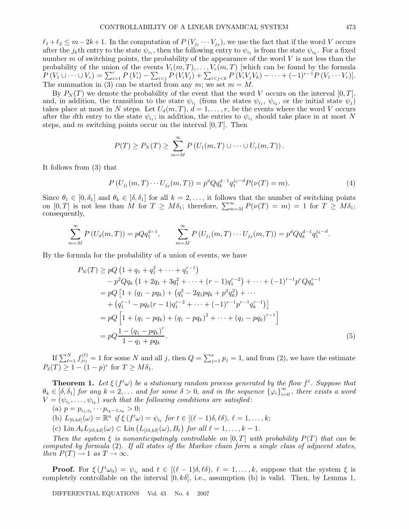
CONTROLLABILITY OF A LINEAR DYNAMICAL SYSTEM 473
1 + 2 ≤ m−2k+1. In the computation of P (Vj1 · · ·Vjd), we use the fact that if the word V occurs
after the jkth entry to the state ψi1 , then the following entry to ψi1 is from the state ψik. For a fixed
number m of switching points, the probability of the appearance of the word V is not less than theprobability of the union of the events V1(m,T ), . . . , Vr(m,T ) [which can be found by the formulaP (V1 ∪ · · · ∪ Vr) =
∑r
i=1 P (Vi) −∑
i<j P (ViVj) +∑
i<j<k P (ViVjVk) − · · · + (−1)r−1P (V1 · · ·Vr)].The summation in (3) can be started from any m; we set m = M .
By PN (T ) we denote the probability of the event that the word V occurs on the interval [0, T ],and, in addition, the transition to the state ψi1 (from the states ψi1 , ψik
, or the initial state ψj)takes place at most in N steps. Let Ud(m,T ), d = 1, . . . , r, be the events where the word V occursafter the dth entry to the state ψi1 ; in addition, the entries to ψi1 should take place in at most Nsteps, and m switching points occur on the interval [0, T ]. Then
P (T ) ≥ PN (T ) ≥∞∑
m=M
P (U1(m,T ) ∪ · · · ∪ Ur(m,T )) .
It follows from (3) that
P (Uj1(m,T ) · · ·Ujd(m,T )) = pdQqd−1
k qjd−d1 P (ν(T ) = m). (4)
Since θ1 ∈ [0, δ1] and θk ∈ [δ, δ1] for all k = 2, . . . , it follows that the number of switching pointson [0, T ] is not less than M for T ≥ Mδ1; therefore,
∑∞m=M P (ν(T ) = m) = 1 for T ≥ Mδ1;
consequently,
∞∑
m=M
P (Ud(m,T )) = pQqd−11 ,
∞∑
m=M
P (Uj1(m,T ) · · ·Ujd(m,T )) = pdQqd−1
k qjd−d1 .
By the formula for the probability of a union of events, we have
PN(T ) ≥ pQ(1 + q1 + q2
1 + · · · + qr−11
)
− p2Qqk
(1 + 2q1 + 3q2
1 + · · · + (r − 1)qr−21
)+ · · · + (−1)r−1prQqr−1
k
= pQ[1 + (q1 − pqk) +
(q21 − 2q1pqk + p2q2
k
)+ · · ·
+(qr−11 − pqk(r − 1)qr−2
1 + · · · + (−1)r−1pr−1qr−1k
)]
= pQ[1 + (q1 − pqk) + (q1 − pqk)
2 + · · · + (q1 − pqk)r−1
]
= pQ1 − (q1 − pqk)
r
1 − q1 + pqk
. (5)
If∑N
�=1 f(�)ji1
= 1 for some N and all j, then Q =∑s
j=1 pj = 1, and from (2), we have the estimatePδ(T ) ≥ 1 − (1 − p)r for T ≥ Mδ1.
Theorem 1. Let ξ (f tω) be a stationary random process generated by the flow f t. Suppose thatθk ∈ [δ, δ1] for any k = 2, . . . and for some δ > 0, and in the sequence {ϕi}∞i=0 , there exists a wordV = (ψi1 , . . . , ψik
) such that the following conditions are satisfied :(a) p = pi1,i2 · · · pik−1,ik
> 0;(b) L[0,kδ](ω) = R
n if ξ (f tω) = ψi�for t ∈ [( − 1)δ, δ), = 1, . . . , k;
(c) Lin A�L[�δ,kδ](ω) ⊂ Lin(L[�δ,kδ](ω), B�
)for all = 1, . . . , k − 1.
Then the system ξ is nonanticipatingly controllable on [0, T ] with probability P (T ) that can becomputed by formula (2). If all states of the Markov chain form a single class of adjacent states,then P (T ) → 1 as T → ∞.
Proof. For ξ (f tω0) = ψi�and t ∈ [( − 1)δ, δ), = 1, . . . , k, suppose that the system ξ is
completely controllable on the interval [0, kδ], i.e., assumption (b) is valid. Then, by Lemma 1,
DIFFERENTIAL EQUATIONS Vol. 43 No. 4 2007
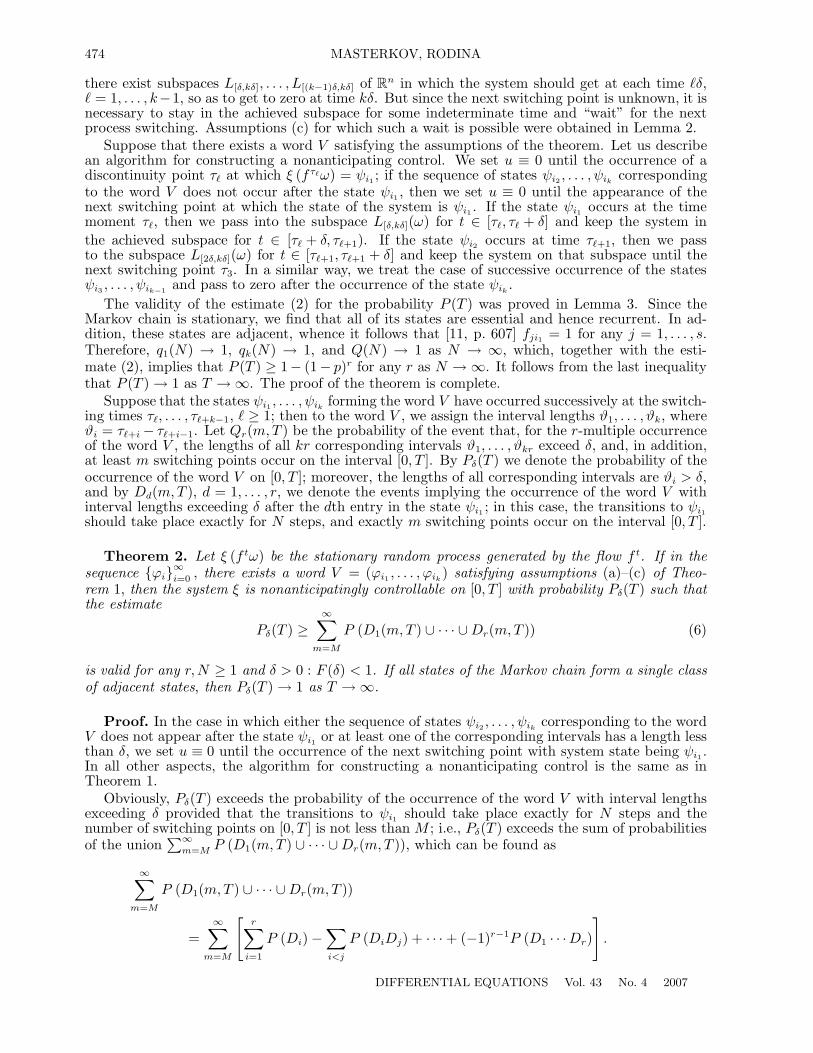
474 MASTERKOV, RODINA
there exist subspaces L[δ,kδ], . . . , L[(k−1)δ,kδ] of Rn in which the system should get at each time δ,
= 1, . . . , k−1, so as to get to zero at time kδ. But since the next switching point is unknown, it isnecessary to stay in the achieved subspace for some indeterminate time and “wait” for the nextprocess switching. Assumptions (c) for which such a wait is possible were obtained in Lemma 2.
Suppose that there exists a word V satisfying the assumptions of the theorem. Let us describean algorithm for constructing a nonanticipating control. We set u ≡ 0 until the occurrence of adiscontinuity point τ� at which ξ (f τ�ω) = ψi1 ; if the sequence of states ψi2 , . . . , ψik
correspondingto the word V does not occur after the state ψi1 , then we set u ≡ 0 until the appearance of thenext switching point at which the state of the system is ψi1 . If the state ψi1 occurs at the timemoment τ�, then we pass into the subspace L[δ,kδ](ω) for t ∈ [τ�, τ� + δ] and keep the system inthe achieved subspace for t ∈ [τ� + δ, τ�+1). If the state ψi2 occurs at time τ�+1, then we passto the subspace L[2δ,kδ](ω) for t ∈ [τ�+1, τ�+1 + δ] and keep the system on that subspace until thenext switching point τ3. In a similar way, we treat the case of successive occurrence of the statesψi3 , . . . , ψik−1 and pass to zero after the occurrence of the state ψik
.The validity of the estimate (2) for the probability P (T ) was proved in Lemma 3. Since the
Markov chain is stationary, we find that all of its states are essential and hence recurrent. In ad-dition, these states are adjacent, whence it follows that [11, p. 607] fji1 = 1 for any j = 1, . . . , s.Therefore, q1(N) → 1, qk(N) → 1, and Q(N) → 1 as N → ∞, which, together with the esti-mate (2), implies that P (T ) ≥ 1− (1− p)r for any r as N → ∞. It follows from the last inequalitythat P (T ) → 1 as T → ∞. The proof of the theorem is complete.
Suppose that the states ψi1 , . . . , ψikforming the word V have occurred successively at the switch-
ing times τ�, . . . , τ�+k−1, ≥ 1; then to the word V , we assign the interval lengths ϑ1, . . . , ϑk, whereϑi = τ�+i − τ�+i−1. Let Qr(m,T ) be the probability of the event that, for the r-multiple occurrenceof the word V , the lengths of all kr corresponding intervals ϑ1, . . . , ϑkr exceed δ, and, in addition,at least m switching points occur on the interval [0, T ]. By Pδ(T ) we denote the probability of theoccurrence of the word V on [0, T ]; moreover, the lengths of all corresponding intervals are ϑi > δ,and by Dd(m,T ), d = 1, . . . , r, we denote the events implying the occurrence of the word V withinterval lengths exceeding δ after the dth entry in the state ψi1 ; in this case, the transitions to ψi1should take place exactly for N steps, and exactly m switching points occur on the interval [0, T ].
Theorem 2. Let ξ (f tω) be the stationary random process generated by the flow f t. If in thesequence {ϕi}∞i=0 , there exists a word V = (ϕi1 , . . . , ϕik
) satisfying assumptions (a)–(c) of Theo-rem 1, then the system ξ is nonanticipatingly controllable on [0, T ] with probability Pδ(T ) such thatthe estimate
Pδ(T ) ≥∞∑
m=M
P (D1(m,T ) ∪ · · · ∪ Dr(m,T )) (6)
is valid for any r,N ≥ 1 and δ > 0 : F (δ) < 1. If all states of the Markov chain form a single classof adjacent states, then Pδ(T ) → 1 as T → ∞.
Proof. In the case in which either the sequence of states ψi2 , . . . , ψikcorresponding to the word
V does not appear after the state ψi1 or at least one of the corresponding intervals has a length lessthan δ, we set u ≡ 0 until the occurrence of the next switching point with system state being ψi1 .In all other aspects, the algorithm for constructing a nonanticipating control is the same as inTheorem 1.
Obviously, Pδ(T ) exceeds the probability of the occurrence of the word V with interval lengthsexceeding δ provided that the transitions to ψi1 should take place exactly for N steps and thenumber of switching points on [0, T ] is not less than M ; i.e., Pδ(T ) exceeds the sum of probabilitiesof the union
∑∞m=M P (D1(m,T ) ∪ · · · ∪ Dr(m,T )), which can be found as
∞∑
m=M
P (D1(m,T ) ∪ · · · ∪ Dr(m,T ))
=∞∑
m=M
[r∑
i=1
P (Di) −∑
i<j
P (DiDj) + · · · + (−1)r−1P (D1 · · ·Dr)
]
.
DIFFERENTIAL EQUATIONS Vol. 43 No. 4 2007
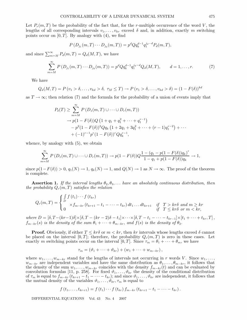
CONTROLLABILITY OF A LINEAR DYNAMICAL SYSTEM 475
Let Pr(m,T ) be the probability of the fact that, for the r-multiple occurrence of the word V , thelengths of all corresponding intervals v1, . . . , vkr exceed δ and, in addition, exactly m switchingpoints occur on [0, T ]. By analogy with (4), we find
P (Dj1(m,T ) · · ·Djd(m,T )) = pdQqd−1
k qjd−d1 Pd(m,T ),
and since∑∞
m=M Pd(m,T ) = Qd(M,T ), we have
∞∑
m=M
P (Dj1(m,T ) · · ·Djd(m,T )) = pdQqd−1
k qjd−d1 Qd(M,T ), d = 1, . . . , r. (7)
We have
Qd(M,T ) = P (v1 > δ, . . . , vkd > δ, τM ≤ T ) → P (v1 > δ, . . . , vkd > δ) = (1 − F (δ))kd
as T → ∞; then relation (7) and the formula for the probability of a union of events imply that
Pδ(T ) ≥∞∑
m=M
P (D1(m,T ) ∪ · · · ∪ Dr(m,T ))
→ p(1 − F (δ))Q(1 + q1 + q2
1 + · · · + qr−11
)
− p2(1 − F (δ))2Qqk
(1 + 2q1 + 3q2
1 + · · · + (r − 1)qr−21
)+ · · ·
+ (−1)r−1pr(1 − F (δ))rQqr−1k ,
whence, by analogy with (5), we obtain
∞∑
m=M
P (D1(m,T ) ∪ · · · ∪ Dr(m,T )) → p(1 − F (δ))Q1 − (q1 − p(1 − F (δ))qk)
r
1 − q1 + p(1 − F (δ))qk
→ 1,
since p(1−F (δ)) > 0, q1(N) → 1, qk(N) → 1, and Q(N) → 1 as N → ∞. The proof of the theoremis complete.
Assertion 1. If the interval lengths θ2, θ3, . . . have an absolutely continuous distribution, thenthe probability Qr(m,T ) satisfies the relation
Qr(m,T ) =
⎧⎨
⎩
∫
D
f (t1) · · · f (tkr)
×fm−kr (tkr+1 − t1 − · · · − tkr) dt1 . . . dtkr+1 if T > krδ and m ≥ kr0 if T ≤ krδ or m < kr,
where D = [δ, T−(kr−1)δ]×[δ, T − (kr − 2)δ − t1]×· · ·×[δ, T − t1 − · · · − tkr−1]×[t1 + · · · + tkr, T ] ,fm−kr(s) is the density of the sum θ1 + · · · + θm−kr, and f(s) is the density of θ2.
Proof. Obviously, if either T ≤ krδ or m < kr, then kr intervals whose lengths exceed δ cannotbe placed on the interval [0, T ]; therefore, the probability Qr(m,T ) is zero in these cases. Letexactly m switching points occur on the interval [0, T ]. Since τm = θ1 + · · · + θm, we have
τm = (ϑ1 + · · · + ϑkr) + (w1 + · · · + wm−kr) ,
where w1, . . . , wm−kr stand for the lengths of intervals not occurring in r words V . Since w1, . . . ,wm−kr are independent variables and have the same distribution as θ1, . . . , θm−kr, it follows thatthe density of the sum w1, . . . , wm−kr coincides with the density fm−kr(t) and can be evaluated byconvolution formulas [11, p. 258]. For fixed ϑ1, . . . , ϑkr the density of the conditional distributionof τm is equal to fm−kr (tkr+1 − t1 − · · · − tkr); and since ϑ1, . . . , ϑkr are independent, it follows thatthe mutual density of the variables ϑ1, . . . , ϑkr, τm is equal to
f (t1, . . . , tkr+1) = f (t1) · · · f (tkr) fm−kr (tkr+1 − t1 − · · · − tkr) .
DIFFERENTIAL EQUATIONS Vol. 43 No. 4 2007
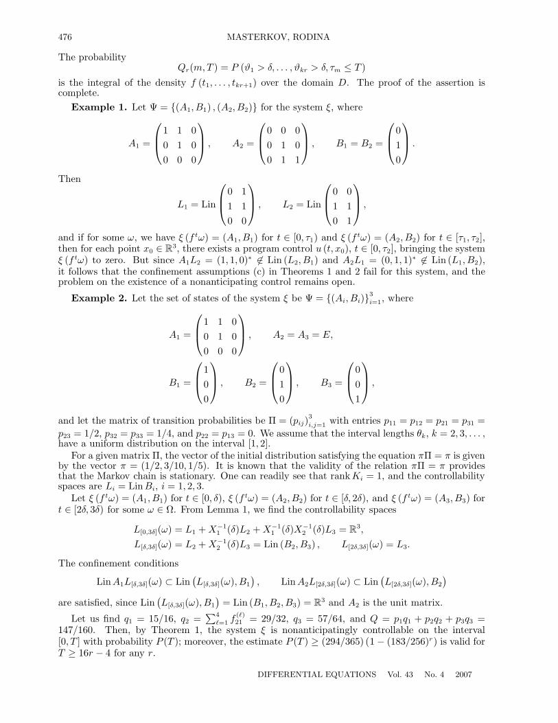
476 MASTERKOV, RODINA
The probabilityQr(m,T ) = P (ϑ1 > δ, . . . , ϑkr > δ, τm ≤ T )
is the integral of the density f (t1, . . . , tkr+1) over the domain D. The proof of the assertion iscomplete.
Example 1. Let Ψ = {(A1, B1) , (A2, B2)} for the system ξ, where
A1 =
⎛
⎜⎝
1 1 00 1 00 0 0
⎞
⎟⎠ , A2 =
⎛
⎜⎝
0 0 00 1 00 1 1
⎞
⎟⎠ , B1 = B2 =
⎛
⎜⎝
010
⎞
⎟⎠ .
Then
L1 = Lin
⎛
⎜⎝
0 11 10 0
⎞
⎟⎠ , L2 = Lin
⎛
⎜⎝
0 01 10 1
⎞
⎟⎠ ,
and if for some ω, we have ξ (f tω) = (A1, B1) for t ∈ [0, τ1) and ξ (f tω) = (A2, B2) for t ∈ [τ1, τ2],then for each point x0 ∈ R
3, there exists a program control u (t, x0), t ∈ [0, τ2], bringing the systemξ (f tω) to zero. But since A1L2 = (1, 1, 0)∗ �∈ Lin (L2, B1) and A2L1 = (0, 1, 1)∗ �∈ Lin (L1, B2),it follows that the confinement assumptions (c) in Theorems 1 and 2 fail for this system, and theproblem on the existence of a nonanticipating control remains open.
Example 2. Let the set of states of the system ξ be Ψ = {(Ai, Bi)}3
i=1, where
A1 =
⎛
⎜⎝
1 1 00 1 00 0 0
⎞
⎟⎠ , A2 = A3 = E,
B1 =
⎛
⎜⎝
100
⎞
⎟⎠ , B2 =
⎛
⎜⎝
010
⎞
⎟⎠ , B3 =
⎛
⎜⎝
001
⎞
⎟⎠ ,
and let the matrix of transition probabilities be Π = (pij)3
i,j=1 with entries p11 = p12 = p21 = p31 =p23 = 1/2, p32 = p33 = 1/4, and p22 = p13 = 0. We assume that the interval lengths θk, k = 2, 3, . . . ,have a uniform distribution on the interval [1, 2].
For a given matrix Π, the vector of the initial distribution satisfying the equation πΠ = π is givenby the vector π = (1/2, 3/10, 1/5). It is known that the validity of the relation πΠ = π providesthat the Markov chain is stationary. One can readily see that rankKi = 1, and the controllabilityspaces are Li = LinBi, i = 1, 2, 3.
Let ξ (f tω) = (A1, B1) for t ∈ [0, δ), ξ (f tω) = (A2, B2) for t ∈ [δ, 2δ), and ξ (f tω) = (A3, B3) fort ∈ [2δ, 3δ) for some ω ∈ Ω. From Lemma 1, we find the controllability spaces
L[0,3δ](ω) = L1 + X−11 (δ)L2 + X−1
1 (δ)X−12 (δ)L3 = R
3,
L[δ,3δ](ω) = L2 + X−12 (δ)L3 = Lin (B2, B3) , L[2δ,3δ](ω) = L3.
The confinement conditions
LinA1L[δ,3δ](ω) ⊂ Lin(L[δ,3δ](ω), B1
), Lin A2L[2δ,3δ](ω) ⊂ Lin
(L[2δ,3δ](ω), B2
)
are satisfied, since Lin(L[δ,3δ](ω), B1
)= Lin (B1, B2, B3) = R
3 and A2 is the unit matrix.
Let us find q1 = 15/16, q2 =∑4
�=1 f(�)21 = 29/32, q3 = 57/64, and Q = p1q1 + p2q2 + p3q3 =
147/160. Then, by Theorem 1, the system ξ is nonanticipatingly controllable on the interval[0, T ] with probability P (T ); moreover, the estimate P (T ) ≥ (294/365) (1 − (183/256)r) is valid forT ≥ 16r − 4 for any r.
DIFFERENTIAL EQUATIONS Vol. 43 No. 4 2007
CONTROLLABILITY OF A LINEAR DYNAMICAL SYSTEM 477
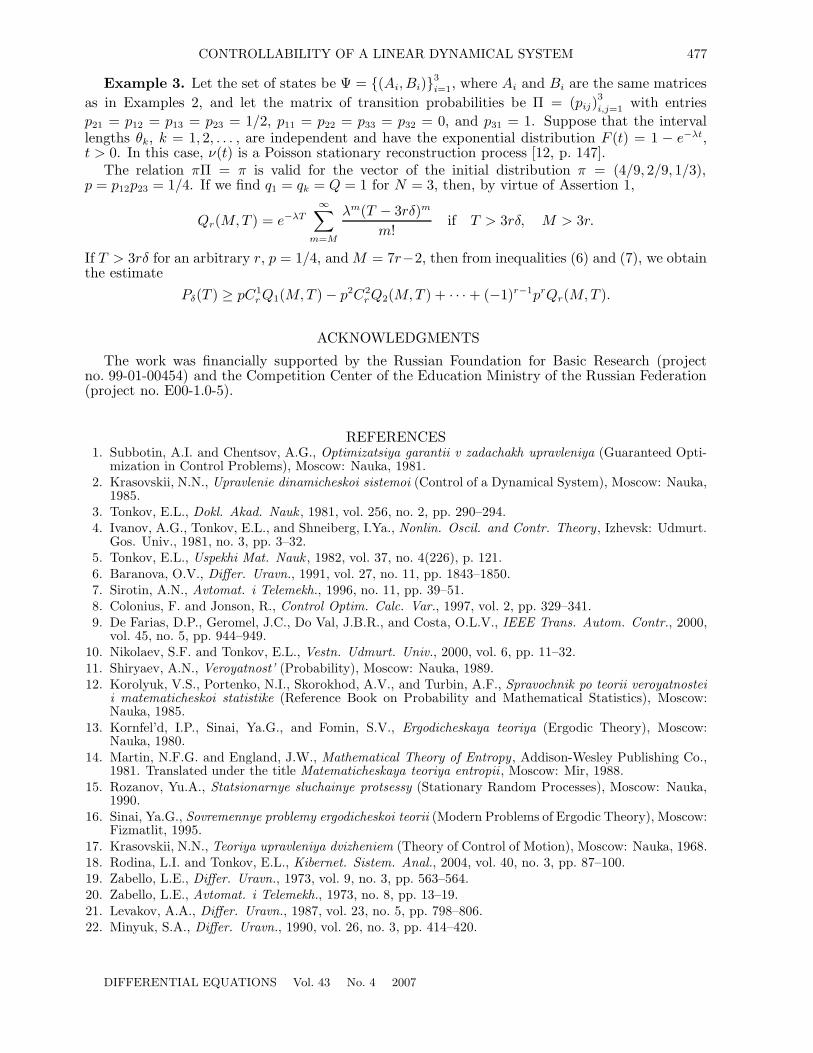
Example 3. Let the set of states be Ψ = {(Ai, Bi)}3
i=1, where Ai and Bi are the same matricesas in Examples 2, and let the matrix of transition probabilities be Π = (pij)
3
i,j=1 with entriesp21 = p12 = p13 = p23 = 1/2, p11 = p22 = p33 = p32 = 0, and p31 = 1. Suppose that the intervallengths θk, k = 1, 2, . . . , are independent and have the exponential distribution F (t) = 1 − e−λt,t > 0. In this case, ν(t) is a Poisson stationary reconstruction process [12, p. 147].
The relation πΠ = π is valid for the vector of the initial distribution π = (4/9, 2/9, 1/3),p = p12p23 = 1/4. If we find q1 = qk = Q = 1 for N = 3, then, by virtue of Assertion 1,
Qr(M,T ) = e−λT
∞∑
m=M
λm(T − 3rδ)m
m!if T > 3rδ, M > 3r.
If T > 3rδ for an arbitrary r, p = 1/4, and M = 7r−2, then from inequalities (6) and (7), we obtainthe estimate
Pδ(T ) ≥ pC1r Q1(M,T ) − p2C2
r Q2(M,T ) + · · · + (−1)r−1prQr(M,T ).
ACKNOWLEDGMENTS
The work was financially supported by the Russian Foundation for Basic Research (projectno. 99-01-00454) and the Competition Center of the Education Ministry of the Russian Federation(project no. E00-1.0-5).
REFERENCES1. Subbotin, A.I. and Chentsov, A.G., Optimizatsiya garantii v zadachakh upravleniya (Guaranteed Opti-
mization in Control Problems), Moscow: Nauka, 1981.2. Krasovskii, N.N., Upravlenie dinamicheskoi sistemoi (Control of a Dynamical System), Moscow: Nauka,
1985.3. Tonkov, E.L., Dokl. Akad. Nauk , 1981, vol. 256, no. 2, pp. 290–294.4. Ivanov, A.G., Tonkov, E.L., and Shneiberg, I.Ya., Nonlin. Oscil. and Contr. Theory, Izhevsk: Udmurt.
Gos. Univ., 1981, no. 3, pp. 3–32.5. Tonkov, E.L., Uspekhi Mat. Nauk , 1982, vol. 37, no. 4(226), p. 121.6. Baranova, O.V., Differ. Uravn., 1991, vol. 27, no. 11, pp. 1843–1850.7. Sirotin, A.N., Avtomat. i Telemekh., 1996, no. 11, pp. 39–51.8. Colonius, F. and Jonson, R., Control Optim. Calc. Var., 1997, vol. 2, pp. 329–341.9. De Farias, D.P., Geromel, J.C., Do Val, J.B.R., and Costa, O.L.V., IEEE Trans. Autom. Contr., 2000,
vol. 45, no. 5, pp. 944–949.10. Nikolaev, S.F. and Tonkov, E.L., Vestn. Udmurt. Univ., 2000, vol. 6, pp. 11–32.11. Shiryaev, A.N., Veroyatnost’ (Probability), Moscow: Nauka, 1989.12. Korolyuk, V.S., Portenko, N.I., Skorokhod, A.V., and Turbin, A.F., Spravochnik po teorii veroyatnostei
i matematicheskoi statistike (Reference Book on Probability and Mathematical Statistics), Moscow:Nauka, 1985.
13. Kornfel’d, I.P., Sinai, Ya.G., and Fomin, S.V., Ergodicheskaya teoriya (Ergodic Theory), Moscow:Nauka, 1980.
14. Martin, N.F.G. and England, J.W., Mathematical Theory of Entropy, Addison-Wesley Publishing Co.,1981. Translated under the title Matematicheskaya teoriya entropii , Moscow: Mir, 1988.
15. Rozanov, Yu.A., Statsionarnye sluchainye protsessy (Stationary Random Processes), Moscow: Nauka,1990.
16. Sinai, Ya.G., Sovremennye problemy ergodicheskoi teorii (Modern Problems of Ergodic Theory), Moscow:Fizmatlit, 1995.
17. Krasovskii, N.N., Teoriya upravleniya dvizheniem (Theory of Control of Motion), Moscow: Nauka, 1968.18. Rodina, L.I. and Tonkov, E.L., Kibernet. Sistem. Anal., 2004, vol. 40, no. 3, pp. 87–100.19. Zabello, L.E., Differ. Uravn., 1973, vol. 9, no. 3, pp. 563–564.20. Zabello, L.E., Avtomat. i Telemekh., 1973, no. 8, pp. 13–19.21. Levakov, A.A., Differ. Uravn., 1987, vol. 23, no. 5, pp. 798–806.22. Minyuk, S.A., Differ. Uravn., 1990, vol. 26, no. 3, pp. 414–420.
DIFFERENTIAL EQUATIONS Vol. 43 No. 4 2007